
Computational Fluid Dynamics: from zero to guruyun.su/science/preview.pdf · Computational Fluid...
44
Computational Fluid Dynamics: from zero to guru Alexander Yun
Transcript of Computational Fluid Dynamics: from zero to guruyun.su/science/preview.pdf · Computational Fluid...
Computational Fluid Dynamics: from zero to guru
Alexander Yun
Computational Fluid Dynamics: from zero to guru
Author: A. Yun, Dr.-Ing., PhD
Technical editors: A. Maltsev, Dr.-Ing. C. Semler, PhD
Editors: V. Makerova O. Varnavskaya, PhD.
Technical consultants: D. Dankin, Dipl. Eng. M. Shcherbakov, Dipl. Eng.
Illustrators: V. Stolyarova O. Sytnik
Typographer: G. Yun
No part of this book may be reprinted, reproduced, transmitted or utilized in any form by any electronical, mechanical photocopying, recording, scanning, or otherwise, without prior written permission of the author. All products names, logos, and brands are the property of their respective owners.

iii
Contents Preface vi Nomenclature viii I Zero level... 0. Welcome or bla-bla-bla! 1 Theoretical part - I 1. The language 4 2. Grammar 11 Practical part - I 3. Mesh and boundary conditions 15 4. First project (WB + CFX) 18 II Beginner and a bit more... 5. Level up! 53 Theoretical part - II 6. Mathematical language 56 7. Conservation laws 67 8. Turbulence 76 9. Simulation based on the statistical averaging 79 9.1. Boussinesq approximation 81 9.2. Algebraic models 83 9.3. One-equation models 88 9.4. Two-equation models 92 9.5. Heat and mixing modeling 106 9.6. Near-wall treatment 107 10. Introduction to structural analysis 114 10.1. Linear static analysis 118 10.2. Nonlinear static analysis 119 10.3. Fatigue 120 10.4. Buckling 128 11. Analytical methods 129 11.1. Hagen-Poiseuille flow 129 11.2. Couette flow 131 11.3. Beam fixed at one end 134 11.4. Column buckling 137 12. Experimental methods for flows and structures 139 12.1. Flow parameters measurements 140 12.2. Structural parameters measurements 146

iv
Practical part - II
13. Geometry creation: Design Modeler, Space Claim 151 14. Mesh generation: ANSYS Mesh 176 15. Solution: Fluent, Icepak, Mechanical 190 16. Post-processing: CFD-Post 252 III Experienced and a bit less... 17. Up, up, up! 258 Theoretical part - III 18. Simulation based on the statistical averaging (cont.) 259 18.1. Nonlinear models 259 18.2. Explicit algebraic Reynolds stress models 262 18.3. Reynolds stress models 270 18.4. Low-Re number effects 277 18.5. Unsteady RANS 283 18.6. Large Eddy Simulation 284 18.7. Hybrid modeling 291 18.8. Direct Numerical Simulation 293 19. Non-Newtonian fluids 298 20. Two-phase flows 304 21. Radiation 311 22. Acoustic 324 23. Electro-magnetism 330 24. Combustion 332 25. Dynamic structure analysis 364 Practical part - III 26. Mesh generation: ICEM CFD 377 27. Solution: Fluent, Rigid Body, Modal, Harmonic 405 28. Post-processing: CFD-Post 434 29. Review of CAD programs 440 30. Review of mesh generation programs 443 31. Review of CFD programs 447 32. Review of structural analysis programs 452 33. Review of post-processing programs 454 34. Review of other programs 456 IV Guru and much less... 35. I know that I know nothing! 459
v
Theoretical part - IV 36. Numerical procedure for flow modeling 461 36.1. Finite volume method 462 36.2. Coordinate transformation 465 36.3. Discretisation form for diffusion term 469 36.4. Discretisation form for convective term 471 36.5. Discretisation form for unsteady term 472 36.6. Discretisation form for source term 473 36.7. Interpolation methods 475 36.8. General system equations 478 36.9. Pressure-velocity coupling 479 36.10. Boundary conditions 483 36.11. Solution method 488 37. Numerical procedure for structural analysis 492 38. Numerical procedure for mesh generation 494 39. Alternative ways to describe turbulence 498 Practical part - IV 40. Solution: FSI, scientific configurations 500 41. Post-processing: Gnuplot 544 42. Open source programs 548 References 552 Name index 564 Demonstration cases index 569 Appendix 572

vi
PREFACE
Computational Fluid Dynamics (CFD) and structural analysis play a significant role in the development of technical devices, building construction, weather predictions, biochemistry processes modeling, and in many other fields. With regard to increase computational power increase and improvements in computer modeling techniques, it is expected that the numerical simulations will prevail the traditional methods, such as the experiments and analytical solutions, in the near future. Behind computer modeling, there are complex mathematical apparatuses, physical theories, chemical reactions, etc. Together, these factors make it difficult to understand and use CFD and structural analysis. This book attempts to systematize and provide an easy explanation of computer modeling.
The book consists of four parts. Each part has two sections: theoretical and practical. The first part represents the absolute beginner level. All explanations are made by words without equations. A simple CFD simulation is introduced in the practical section. The second part has more sophisticated introduction to CFD. The basic equations and theories are considered. The usage of CFD and structural analysis software for general physics is shown in the practical section. The third part gives the information about advanced modeling and introduces different physics, such as combustion, radiation, two-phase flows, acoustics, etc. Simple demonstrations of advanced models, extended physics and review of existed software packages to model flows and structures are shown in the practical section. The last part concentrates on the numerical solution of equations described in previous parts. The practical section has a demonstration of fluid and structure interaction, scientific examples. The important equations, dimensionless numbers and the map of demonstration cases are at the end of book.

vii
The author thanks the technical editors Dr.-Ing. A. Maltsev and Dr. C. Semler for review and helpful comments, editors V. Makerova and Dr. O. Varnavskaya for text correction, technical consultants D. Dankin and M. Shcherbakov who went through all demo cases and made many suggestions and corrections, illustrators V. Stolyarova and O. Sytnik who prepared the illustrations, and typographer G. Yun who typed the text and formulas. The author thanks TU Darmstadt (Germany) for providing the scientific package FASTEST-3D, Simutech Group (Canada) and Dr. C. Semler for ANSYS package, Mentor Graphics (US) and A. Kharitonovich for FloEFD. Many thanks go to Dr. S. Akramov, the Alizadas, G. Drappel, Dr. S. Kim, the Kubekovs, K. Woo, the Zamyatins, and A. Yun Jr. for moral support and advices. Finally, special thanks to my family for continuous support and giving time to write this book.
All recommendations, wishes and corrections please send to email: [email protected].
Alexander Yun
Chapter 0. Welcome or bla-bla-bla!
1
PART I. Zero level...
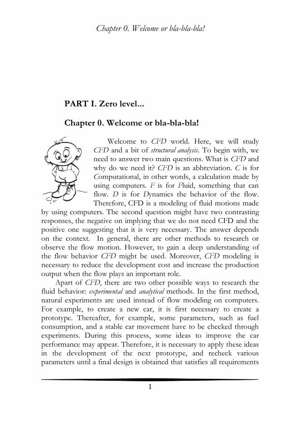
Chapter 0. Welcome or bla-bla-bla!
Welcome to CFD world. Here, we will study CFD and a bit of structural analysis. To begin with, we need to answer two main questions. What is CFD and why do we need it? CFD is an abbreviation. C is for Computational, in other words, a calculation made by using computers. F is for Fluid, something that can flow. D is for Dynamics the behavior of the flow. Therefore, CFD is a modeling of fluid motions made
by using computers. The second question might have two contrasting responses, the negative on implying that we do not need CFD and the positive one suggesting that it is very necessary. The answer depends on the context. In general, there are other methods to research or observe the flow motion. However, to gain a deep understanding of the flow behavior CFD might be used. Moreover, CFD modeling is necessary to reduce the development cost and increase the production output when the flow plays an important role.
Apart of CFD, there are two other possible ways to research the fluid behavior: experimental and analytical methods. In the first method, natural experiments are used instead of flow modeling on computers. For example, to create a new car, it is first necessary to create a prototype. Thereafter, for example, some parameters, such as fuel consumption, and a stable car movement have to be checked through experiments. During this process, some ideas to improve the car performance may appear. Therefore, it is necessary to apply these ideas in the development of the next prototype, and recheck various parameters until a final design is obtained that satisfies all requirements
Chapter 0. Welcome or bla-bla-bla!
2
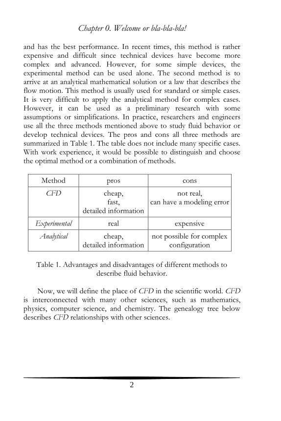
and has the best performance. In recent times, this method is rather expensive and difficult since technical devices have become more complex and advanced. However, for some simple devices, the experimental method can be used alone. The second method is to arrive at an analytical mathematical solution or a law that describes the flow motion. This method is usually used for standard or simple cases. It is very difficult to apply the analytical method for complex cases. However, it can be used as a preliminary research with some assumptions or simplifications. In practice, researchers and engineers use all the three methods mentioned above to study fluid behavior or develop technical devices. The pros and cons all three methods are summarized in Table 1. The table does not include many specific cases. With work experience, it would be possible to distinguish and choose the optimal method or a combination of methods.
Method pros cons
CFD cheap, fast,
detailed information
not real, can have a modeling error
Experimental real expensive
Analytical cheap, detailed information
not possible for complex configuration
Table 1. Advantages and disadvantages of different methods to
describe fluid behavior.
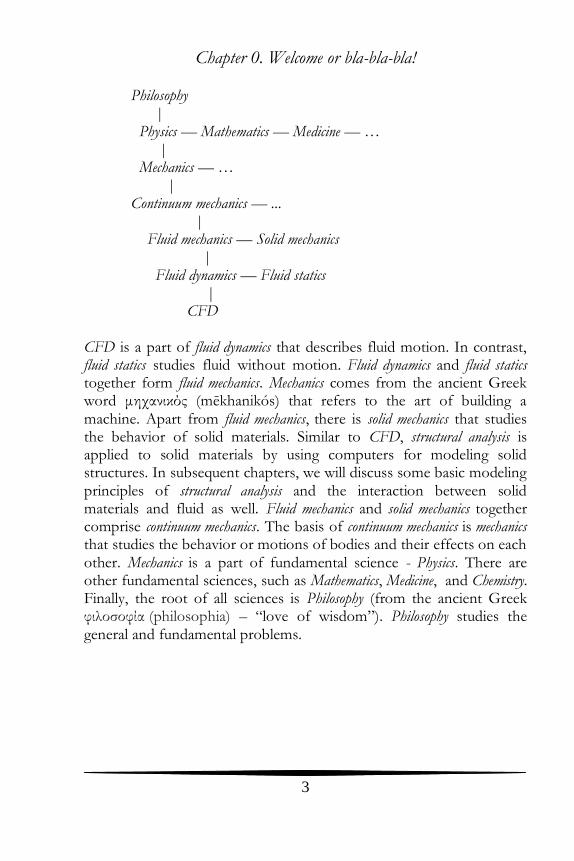
Now, we will define the place of CFD in the scientific world. CFD is interconnected with many other sciences, such as mathematics, physics, computer science, and chemistry. The genealogy tree below describes CFD relationships with other sciences.
Chapter 0. Welcome or bla-bla-bla!
3
Philosophy | Physics — Mathematics — Medicine — … | Mechanics — … | Continuum mechanics — ... | Fluid mechanics — Solid mechanics | Fluid dynamics — Fluid statics | CFD
CFD is a part of fluid dynamics that describes fluid motion. In contrast, fluid statics studies fluid without motion. Fluid dynamics and fluid statics together form fluid mechanics. Mechanics comes from the ancient Greek word μηχανικός (mēkhanikós) that refers to the art of building a machine. Apart from fluid mechanics, there is solid mechanics that studies the behavior of solid materials. Similar to CFD, structural analysis is applied to solid materials by using computers for modeling solid structures. In subsequent chapters, we will discuss some basic modeling principles of structural analysis and the interaction between solid materials and fluid as well. Fluid mechanics and solid mechanics together comprise continuum mechanics. The basis of continuum mechanics is mechanics that studies the behavior or motions of bodies and their effects on each other. Mechanics is a part of fundamental science - Physics. There are other fundamental sciences, such as Mathematics, Medicine, and Chemistry. Finally, the root of all sciences is Philosophy (from the ancient Greek φιλοσοφία (philosophia) – “love of wisdom”). Philosophy studies the general and fundamental problems.

Chapter 1. The language
4
THEORETICAL PART - I Chapter 1. The language
In this chapter we will introduce some of the vocabulary used to describe flow motion. The usage of some of these terms is slightly different from that in common language. There are several basic mathematical and physical terms to be understood. Let us start with simple basic terms that we use very often in our life. To simplify the writing of terms, one or two Latin or Greek letter notations are used. Sometimes, the same letters may be used for different terms. All notations are presented on pages viii to xii.
Velocity is a simple term. It is the rate of movement or how fast a body or flow moves. So, the velocity unit can be expressed in units, such
as meter per second ( ms
), and kilometer per hour ( kmh
). For
convenience, we will use mainly the SI system. SI comes from the French term Syste’me International d’Unite’s (International System of Units). This system has been created to simplify the units system for
international use. The unit of Velocity in SI is meter per second ( ms
).
The Latin letters u , v , and w are usually used to denote velocity. Mass has many definitions. We will use a simple one that defines mass as the amount of matter. Sometimes mass is confused with weight. Unlike mass, weight is the force that a body exerts to maintain its position against gravitational force. So, the mass of body on the Earth or on the Moon would be equivalent, but the weight would be different since the gravitational force is not the same on both bodies. Mass unit
in SI is a kilogram ( kg ), and it is denoted by the Latin letter m . Mass
flow is more apt for fluid motion. It is the mass of gas or liquid that is passing through a given area in unit time. The unit of mass flow in SI is
a kilogram per second ( kgs
). A similar term is volume flow. It is the
volume of fluid that passes through an area. This parameter is often used to evaluate fans. Instead of the SI unit a cubic meter per second
Chapter 1. The language
5
(3ms
) the unit cubic feet per second (CFM) is often used in the
electronic industry. Another basic term is a density. It is defined as a mass per cubic meter
( 3kg
m). The Greek letter is used to denote density.
For time, we will use a simple common definition: time is just time and it always progresses in one direction. The unit of time in SI is a second ( s ) and it is usually denoted by Latin letter t . Temperature is the measure of the heat of a substance. Different scales are used to measure temperature, including Celsius, Kelvin, and Fahrenheit. In SI, the unit of temperature is Kelvin ( K ). However,
Celsius ( C ) is commonly used as well. To denote temperature, the capital letter T is used. Now, we will look at more abstract terms.
The first term is scalar. Scalar comes from the Latin word – “scalaris” (stepping). Scalar is described by a single number and does not have any other characteristics. Some examples of scalar are length
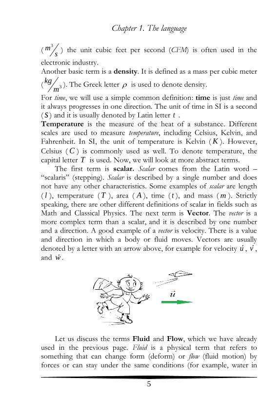
( l ), temperature ( T ), area ( A ), time ( t ), and mass ( m ). Strictly speaking, there are other different definitions of scalar in fields such as Math and Classical Physics. The next term is Vector. The vector is a more complex term than a scalar, and it is described by one number and a direction. A good example of a vector is velocity. There is a value and direction in which a body or fluid moves. Vectors are usually
denoted by a letter with an arrow above, for example for velocity u , v ,
and w .
Let us discuss the terms Fluid and Flow, which we have already used in the previous page. Fluid is a physical term that refers to something that can change form (deform) or flow (fluid motion) by forces or can stay under the same conditions (for example, water in
Chapter 1. The language
6
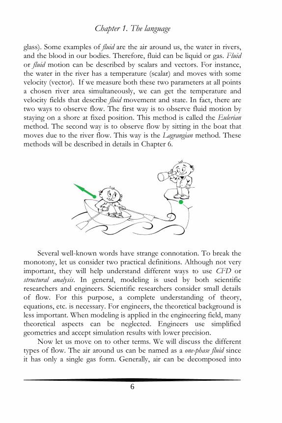
glass). Some examples of fluid are the air around us, the water in rivers, and the blood in our bodies. Therefore, fluid can be liquid or gas. Fluid or fluid motion can be described by scalars and vectors. For instance, the water in the river has a temperature (scalar) and moves with some velocity (vector). If we measure both these two parameters at all points a chosen river area simultaneously, we can get the temperature and velocity fields that describe fluid movement and state. In fact, there are two ways to observe flow. The first way is to observe fluid motion by staying on a shore at fixed position. This method is called the Eulerian method. The second way is to observe flow by sitting in the boat that moves due to the river flow. This way is the Lagrangian method. These methods will be described in details in Chapter 6.
Several well-known words have strange connotation. To break the monotony, let us consider two practical definitions. Although not very important, they will help understand different ways to use CFD or structural analysis. In general, modeling is used by both scientific researchers and engineers. Scientific researchers consider small details of flow. For this purpose, a complete understanding of theory, equations, etc. is necessary. For engineers, the theoretical background is less important. When modeling is applied in the engineering field, many theoretical aspects can be neglected. Engineers use simplified geometries and accept simulation results with lower precision.
Now let us move on to other terms. We will discuss the different types of flow. The air around us can be named as a one-phase fluid since it has only a single gas form. Generally, air can be decomposed into
Chapter 1. The language
7
oxygen (2O ), nitrogen (
2N ), carbon dioxide (2CO ), etc. Such a
composition of same-phase elements is called a multicomponent fluid. If there is a reaction between the chemical elements, for example,
combustion of methane (4CH ) in air (
2O , 2N ,
2CO ), the fluid motion
could be called flow with chemical reactions.
2H , 2O , 2N ,
2CO , etc are the symbolic
representation used in Chemistry to denote
chemical elements. For example, 2H : H means
Hydrogenium (Latin), 2 is the number of atoms
in molecule of Hydrogenium.
Go back to the air around us. In case of rain, we have a two-phase flow: air (gas) and water drops (liquid). Let us consider the burning of wood in CFD terms. The logic is simple. There is wood (solid) and air (gas). Therefore, there are two phases. Wood burns, and so, it means that certain chemical reactions occur. Thus, we get the term two-phase flow with chemical reactions or combustion. In addition, in this case, there is temperature change or heat transfer. So, we might call it: two-phase flow with chemical reactions and heat transfer. It sounds a bit long. The shorter term, two-phase combustion, is used for such cases since the term combustion indicates the occurrence of heat transfer and chemical reactions. Another example of flow with heat transfer is a working computer. There is “cold” surrounding air and “hot” heating chips inside a computer. Sometimes, a simple flow without heat transfer is called “cold” flow. Other possible physics concepts that may be taken into consideration are noise (acoustic), electro-magnetics, radiations, etc. Even if we are talking here about CFD in general, the flow often interacts with solid bodies not only by flow around, but, for example, deforms it. In this case, we have to take such an influence into account. This type of modeling is called Fluid Structure Interaction (FSI). In this case, a structural analysis has to be provided in addition to CFD. In many cases, it is necessary to perform only structural analysis. We will examine some
Chapter 1. The language
8
basic examples of structural analysis in further chapters. Sound knowledge of the definitions of flow type will help navigate in the CFD world freely.
Structural analysis uses Mechanics, Mathematics, Material Science to estimate the deformations, loads, etc. in a structure. This analysis is an important part of mechanical devices development.
Now, let us talk about flow in detail. There are 3 modes of flow:
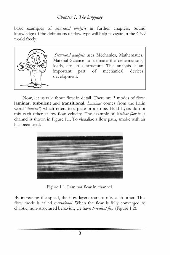
laminar, turbulent and transitional. Laminar comes from the Latin word “lamina”, which refers to a plate or a stripe. Fluid layers do not mix each other at low-flow velocity. The example of laminar flow in a channel is shown in Figure 1.1. To visualize a flow path, smoke with air has been used.
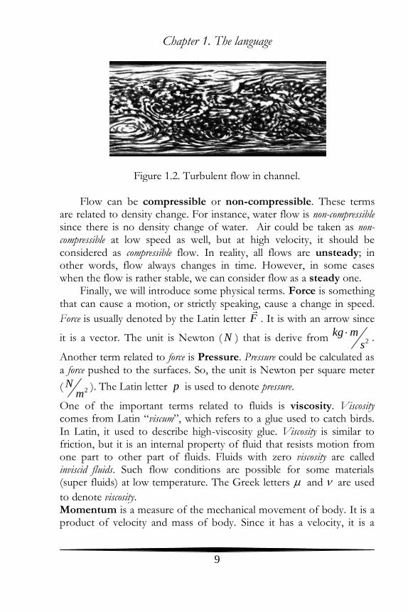
Figure 1.1. Laminar flow in channel. By increasing the speed, the flow layers start to mix each other. This flow mode is called transitional. When the flow is fully converged to chaotic, non-structured behavior, we have turbulent flow (Figure 1.2).
Chapter 1. The language
9
Figure 1.2. Turbulent flow in channel.
Flow can be compressible or non-compressible. These terms are related to density change. For instance, water flow is non-compressible since there is no density change of water. Air could be taken as non-compressible at low speed as well, but at high velocity, it should be considered as compressible flow. In reality, all flows are unsteady; in other words, flow always changes in time. However, in some cases when the flow is rather stable, we can consider flow as a steady one.
Finally, we will introduce some physical terms. Force is something that can cause a motion, or strictly speaking, cause a change in speed.
Force is usually denoted by the Latin letter F . It is with an arrow since
it is a vector. The unit is Newton ( N ) that is derive from 2kg m
s
.
Another term related to force is Pressure. Pressure could be calculated as a force pushed to the surfaces. So, the unit is Newton per square meter
( 2N
m). The Latin letter p is used to denote pressure.
One of the important terms related to fluids is viscosity. Viscosity comes from Latin “viscum”, which refers to a glue used to catch birds. In Latin, it used to describe high-viscosity glue. Viscosity is similar to friction, but it is an internal property of fluid that resists motion from one part to other part of fluids. Fluids with zero viscosity are called inviscid fluids. Such flow conditions are possible for some materials (super fluids) at low temperature. The Greek letters and are used
to denote viscosity. Momentum is a measure of the mechanical movement of body. It is a product of velocity and mass of body. Since it has a velocity, it is a
Chapter 1. The language
10
vector as well. Let us explain it in other words. There are two balls with identical shape, but one of them is made of steel and the other one is of plastic. If we roll them and get the same speed for both balls, the steel ball will roll further than the plastic ball after releasing as it has more mass. We can say that the steel ball has more momentum. In fact, we need to apply more force to the steel ball than to the plastic one to achieve the same speed. Another thing is that if we take two identical steel balls and roll one with higher speed than other; the higher speed ball will roll further. So, in this case, velocity and mass can be interchangeable. If we create the same momentum for different balls, they
will move the same distance, for example, 2 kg ball with 3 ms
and 3
kg ball with 2 ms
.

Chapter 2. Grammar
11
Chapter 2. Grammar
Now we are coming to a more complex area: grammar of CFD. To describe a fluid motion, certain equations have to be solved. In this chapter, we will discuss the main equations in words. In Math, the
equations are usually abstract (not real). For instance, A plus unknown number X is equivalent to B . It is an equation. So, to find unknown
number X , we need to subtract A from B . This action is a solution. There is no physical meaning behind this equation except other than the value of the numbers. If we put some objects such as apples behind the numbers, it would be more realistic. Similarly, if we add some physical meaning, such as velocity and density to numbers, we might get the equations that describe some physical processes, for example, a fluid motion.
Physical processes can be described by laws. Equations are the mathematical formulation of laws. Laws and equations together create the CFD grammar. The basis of CFD is the conservation laws. Let us discuss them. The first law is mass conservation. This law is easy to understand. For instance, there is a 1 liter bottle of water, and we fill a 0.2 liter glass from this bottle; thus, we have 0.8 liter of water in the bottle and 0.2 liter in the glass. The total amount of water remains the same, at 1 liter. Now, there is a real case that is more closed to fluid motion. Take a channel system with two supplies and one exit; introduce 2 liters per second into one and 3 liters per second into the other supplier. Thus, we will get 5 liters per second at the exit. In general, the total mass flow at the exit will be the total of the mass flowing at the suppliers (Figure 2.1).
Figure 2.1. Mass flows in the channel.
Chapter 2. Grammar
12
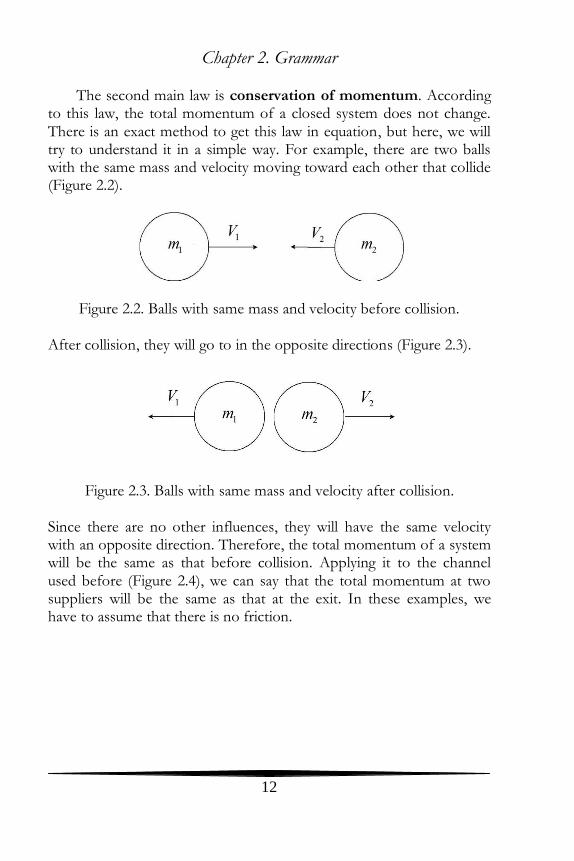
The second main law is conservation of momentum. According to this law, the total momentum of a closed system does not change. There is an exact method to get this law in equation, but here, we will try to understand it in a simple way. For example, there are two balls with the same mass and velocity moving toward each other that collide (Figure 2.2).
Figure 2.2. Balls with same mass and velocity before collision. After collision, they will go to in the opposite directions (Figure 2.3).
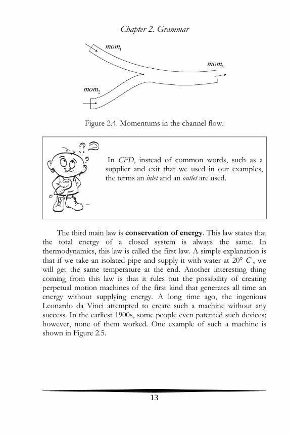
Figure 2.3. Balls with same mass and velocity after collision. Since there are no other influences, they will have the same velocity with an opposite direction. Therefore, the total momentum of a system will be the same as that before collision. Applying it to the channel used before (Figure 2.4), we can say that the total momentum at two suppliers will be the same as that at the exit. In these examples, we have to assume that there is no friction.
Chapter 2. Grammar
13
Figure 2.4. Momentums in the channel flow.
In CFD, instead of common words, such as a supplier and exit that we used in our examples, the terms an inlet and an outlet are used.
The third main law is conservation of energy. This law states that
the total energy of a closed system is always the same. In thermodynamics, this law is called the first law. A simple explanation is
that if we take an isolated pipe and supply it with water at 20° С , we will get the same temperature at the end. Another interesting thing coming from this law is that it rules out the possibility of creating perpetual motion machines of the first kind that generates all time an energy without supplying energy. A long time ago, the ingenious Leonardo da Vinci attempted to create such a machine without any success. In the earliest 1900s, some people even patented such devices; however, none of them worked. One example of such a machine is shown in Figure 2.5.

Chapter 2. Grammar
14
Figure 2.5. A perpetual motion machine.
The geometry of cogs is created to have the balls on the left side more closed to the axis than on the right side. Therefore, we might think that it will rotate since the leverage seems lower on left than on the right side, but in reality, the wheel will be without any motion as the forces on the left and right sides are balanced by the different number of balls.
There are 2 other types of perpetual motion machines. These machines break other thermodynamic laws. One law says that all processes in nature are not reversible, and another says that all processes occur with losses, such as by friction or energy dissipation.
The above conservation laws are valid for isolated (closed) systems where there is no interaction with the surrounding environment, for example, heat loss through channel walls, friction between balls and ground, etc. The isolated systems are not possible in real life. However, in many cases the interaction with environment can be neglected and the system can be considered as isolated one. The three fundamental conservative laws are valid not only for CFD, but for all other sciences. Now, we are ready to move to a practical part.

Chapter 8.Turbulence
76
Chapter 8. Turbulence
A majority of flows in technical applications are rather turbulent than laminar. Peter Bradshaw in his introduction to Turbulence wrote: “the one uncontroversial fact about turbulence is that it is the most complicated kind of fluid motion”.
Since 1883, following Osborne Reynolds, it has been possible to characterize the state of flow using Reynolds number:
0 0Rel u
, (8.1)
where 0l is a typical length, 0u a typical bulk velocity and a
kinematic viscosity. The Reynolds number expresses the ratio between inertial and viscous (or molecular) forces. If this ratio is small, the viscous (or molecular) forces are comparable to the inertial forces and the flow keeps its regular structure (laminar flow). If the ratio becomes larger, the viscous forces do not suffice to compensate the inertial forces. The flow turns unstable, and small initial perturbations destroy the regular flow structure, causing turbulence (turbulent flow). The turbulent flows can be imagined as collections of eddies. Turbulence increases the rate at which conserved quantities are stirred, i. e., parcels of fluid with different contents of conserved quantity (momentum, energy, concentration, etc.) are brought into contact. This is often called turbulent mixing or turbulent diffusion. The molecular viscosity reduces the velocity gradients, causing a destruction of turbulent eddies and a dissipation of kinetic energy into the internal energy of fluid. The bigger eddies dissipate into smaller ones, transferring the kinetic energy of turbulent fluctuations. This process, first revealed by Kolmogorov [54], is called energy cascade. Small eddies can form into a bigger one as well. This reverse process is called back scattering. Richardson (1922) wrote a small poem describing the cascade character of turbulence:
Big whirls make little whirls, That feed on their velocity;
Little whirls have smaller ones, And so on into viscosity.
Chapter 8.Turbulence
77
Recent investigations have shown the turbulent flows of coherent structures as repeatable and essentially of deterministic character. The random part that is dominant in turbulent flows causes these events to differ in size, strength, and time interval between occurrences. There are, however, some flows that feature coherent structures with clear periodicity, and certain frequency can be referred to such a periodical motion. To summarize, it appears clearly that turbulent flows are:
- random in time and space
- unsteady
- three-dimensional
- dissipative
- vortical. It is possible to describe the turbulent motion by laws of probability
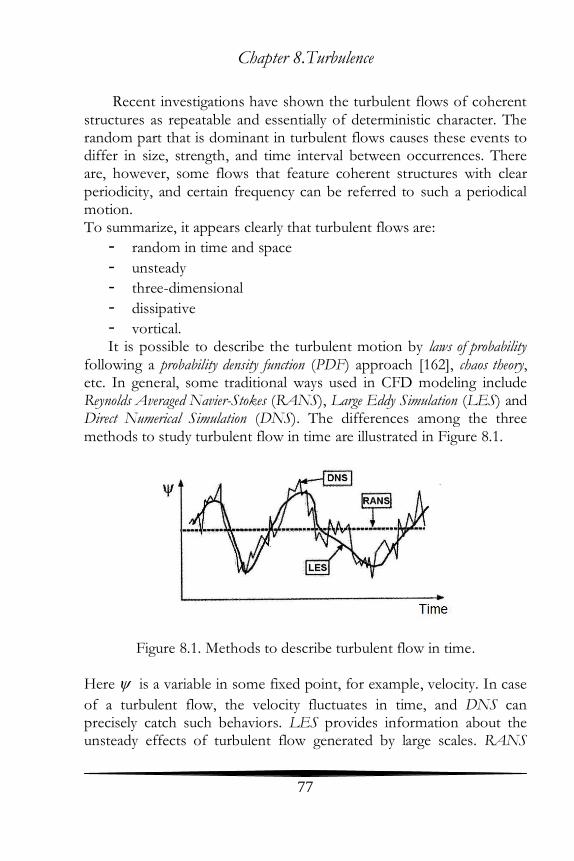
following a probability density function (PDF) approach [162], chaos theory, etc. In general, some traditional ways used in CFD modeling include Reynolds Averaged Navier-Stokes (RANS), Large Eddy Simulation (LES) and Direct Numerical Simulation (DNS). The differences among the three methods to study turbulent flow in time are illustrated in Figure 8.1.
Figure 8.1. Methods to describe turbulent flow in time. Here is a variable in some fixed point, for example, velocity. In case
of a turbulent flow, the velocity fluctuates in time, and DNS can precisely catch such behaviors. LES provides information about the unsteady effects of turbulent flow generated by large scales. RANS
Chapter 8.Turbulence
78
operates with averaged data. To model the transient effects in RANS, the unsteady RANS (URANS) can be used [170]. The URANS method will be described in Chapter 18.5. The alternative methods to describe turbulent flows will be considered in part IV.
Chapter 14.Mesh generation: ANSYS Mesh
176
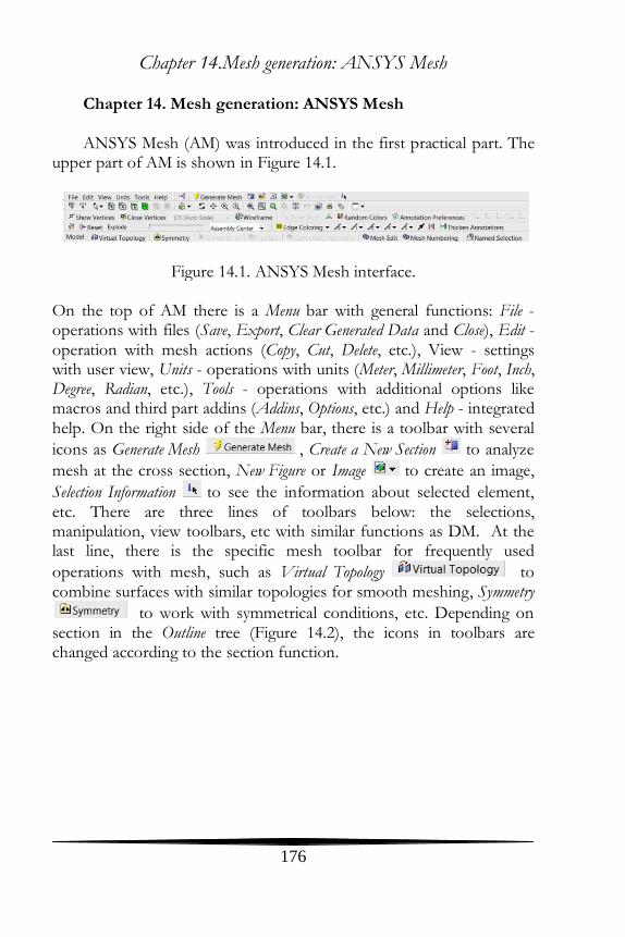
Chapter 14. Mesh generation: ANSYS Mesh ANSYS Mesh (AM) was introduced in the first practical part. The
upper part of AM is shown in Figure 14.1.
Figure 14.1. ANSYS Mesh interface. On the top of AM there is a Menu bar with general functions: File - operations with files (Save, Export, Clear Generated Data and Close), Edit - operation with mesh actions (Copy, Cut, Delete, etc.), View - settings with user view, Units - operations with units (Meter, Millimeter, Foot, Inch, Degree, Radian, etc.), Tools - operations with additional options like macros and third part addins (Addins, Options, etc.) and Help - integrated help. On the right side of the Menu bar, there is a toolbar with several
icons as Generate Mesh , Create a New Section to analyze
mesh at the cross section, New Figure or Image to create an image,
Selection Information to see the information about selected element, etc. There are three lines of toolbars below: the selections, manipulation, view toolbars, etc with similar functions as DM. At the last line, there is the specific mesh toolbar for frequently used
operations with mesh, such as Virtual Topology to combine surfaces with similar topologies for smooth meshing, Symmetry
to work with symmetrical conditions, etc. Depending on section in the Outline tree (Figure 14.2), the icons in toolbars are changed according to the section function.
Chapter 14.Mesh generation: ANSYS Mesh
177
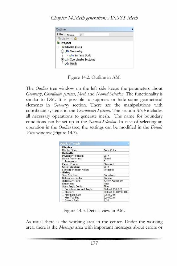
Figure 14.2. Outline in AM. The Outline tree window on the left side keeps the parameters about Geometry, Coordinate systems, Mesh and Named Selection. The functionality is similar to DM. It is possible to suppress or hide some geometrical elements in Geometry section. There are the manipulations with coordinate systems in the Coordinates Systems. The section Mesh includes all necessary operations to generate mesh. The name for boundary conditions can be set up in the Named Selection. In case of selecting an operation in the Outline tree, the settings can be modified in the Details View window (Figure 14.3).
Figure 14.3. Details view in AM. As usual there is the working area in the center. Under the working area, there is the Messages area with important messages about errors or

Chapter 14.Mesh generation: ANSYS Mesh
178
recommendations during meshing process. Finally, on the bottom there is the Status bar that shows a current state and some geometrical information. Let us generate a mesh for 2D/3D Ahmed body.
Prerequisites Software: Workbench, Ansys Mesh (ANSYS 17.0) Input: 2D/3D CAD models made in Chapter 13 Experience level: beginner
Goal Introduction to ANSYS Mesh (AM)
Description Open the project ahmed_body.wbpj that we created before. We will generate a mesh for this geometry. Take the Mesh in the Component System and drop it to the Geometry cell of Ahmed body 2D in the Project Schematic of WB (Figure 14.4).
Figure 14.4. Attaching Mesh in Workbench.

Chapter 14.Mesh generation: ANSYS Mesh
179
Double-click on the Mesh cell to start AM (Figure 14.5).
Figure 14.5. Starting ANSYS Mesh in WB. First, we will generate the mesh with default parameters. Click on the Mesh in the Outline to see the mesh parameters (Figure 14.3). Click on the Generate button to see the default mesh (Figure 14.6).
Figure 14.6. Default mesh for 2D Ahmed body case. Scale the mesh to see the mesh around Ahmed body. The mesh is not fine enough for aero-dynamic simulations (Figure 14.7).
Figure 14.7. Mesh around Ahmed body.
Chapter 14.Mesh generation: ANSYS Mesh
180
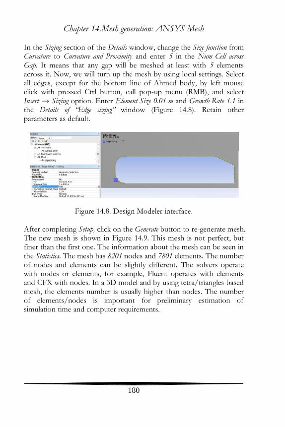
In the Sizing section of the Details window, change the Size function from Curvature to Curvature and Proximity and enter 5 in the Num Cell across Gap. It means that any gap will be meshed at least with 5 elements across it. Now, we will turn up the mesh by using local settings. Select all edges, except for the bottom line of Ahmed body, by left mouse click with pressed Ctrl button, call pop-up menu (RMB), and select Insert → Sizing option. Enter Element Size 0.01 m and Growth Rate 1.1 in the Details of “Edge sizing” window (Figure 14.8). Retain other parameters as default.
Figure 14.8. Design Modeler interface. After completing Setup, click on the Generate button to re-generate mesh. The new mesh is shown in Figure 14.9. This mesh is not perfect, but finer than the first one. The information about the mesh can be seen in the Statistics. The mesh has 8201 nodes and 7801 elements. The number of nodes and elements can be slightly different. The solvers operate with nodes or elements, for example, Fluent operates with elements and CFX with nodes. In a 3D model and by using tetra/triangles based mesh, the elements number is usually higher than nodes. The number of elements/nodes is important for preliminary estimation of simulation time and computer requirements.

Chapter 14.Mesh generation: ANSYS Mesh
181
Figure 14.9. Refined mesh. Select Mesh Metric → Element Quality in the Metric statistic. The minimal Element Quality is relatively low 0.2409. It is possible to check other important quality parameters such as Aspect ratio (Max. = 1.93), Skewness (Max. = 0.72263) and Orthogonal Quality (Min. = 0.64972). The Element Quality option will call the additional Mesh Metrics panel below the Main window (Figure 14.10).
Figure 14.10. Mesh metrics panel. The elements with low quality are not well visible in the Mesh Metrics. Click Control and change the range for X-Axis: Min 0.2 - Max 0.5 and for Y-Axis: Min 0 - Max 10 (Figure 14.11).

Chapter 14.Mesh generation: ANSYS Mesh
182
Figure 14.11. Control panel.
Close the Control panel . Now, the elements with low quality are visible in the Mesh Metrics window. Select all bars (Ctrl + LMB) to see these elements (Figure 14.12).
Figure 14.12. The worst elements.

Chapter 14.Mesh generation: ANSYS Mesh
183
Let us improve it by using other mesh methods. Click on Mesh → Insert → Method (Figure 14.13).
Figure 14.13. Changing the mesh method. Select the Body in the main window for Geometry and method MultiZone Quad/Tri Method in the Details window (Figure 14.14).
Figure 14.14. Setup MultiZone Quad/Tri Method.
Chapter 14.Mesh generation: ANSYS Mesh
184
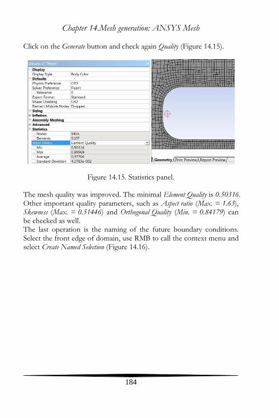
Click on the Generate button and check again Quality (Figure 14.15).
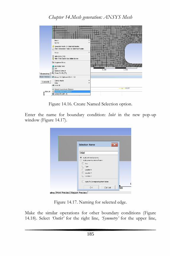
Figure 14.15. Statistics panel. The mesh quality was improved. The minimal Element Quality is 0.50316. Other important quality parameters, such as Aspect ratio (Max. = 1.63), Skewness (Max. = 0.51446) and Orthogonal Quality (Min. = 0.84179) can be checked as well. The last operation is the naming of the future boundary conditions. Select the front edge of domain, use RMB to call the context menu and select Create Named Selection (Figure 14.16).
Chapter 14.Mesh generation: ANSYS Mesh
185
Figure 14.16. Create Named Selection option. Enter the name for boundary condition: Inlet in the new pop-up window (Figure 14.17).
Figure 14.17. Naming for selected edge. Make the similar operations for other boundary conditions (Figure 14.18). Select ‘Outlet’ for the right line, ‘Symmetry’ for the upper line,

Chapter 14.Mesh generation: ANSYS Mesh
186
‘Ground’ for the bottom line, ‘Wall’ for lines limiting Ahmed body and ‘Fluid’ for surface.
Figure 14.18. Setup of names for 2D Ahmed body (cut in X direction). Finally, save the project, close AM and return to WB. Now, we will generate a mesh for 3D Ahmed body. Similar to 2D example, attach the Mesh to Geometry cell in WB and open it. In the Menu bar, change the View to Wireframe to see the inside geometry (Figure 14.19).
Figure 14.19. Wireframe view for 3D Ahmed body.
Chapter 14.Mesh generation: ANSYS Mesh
187
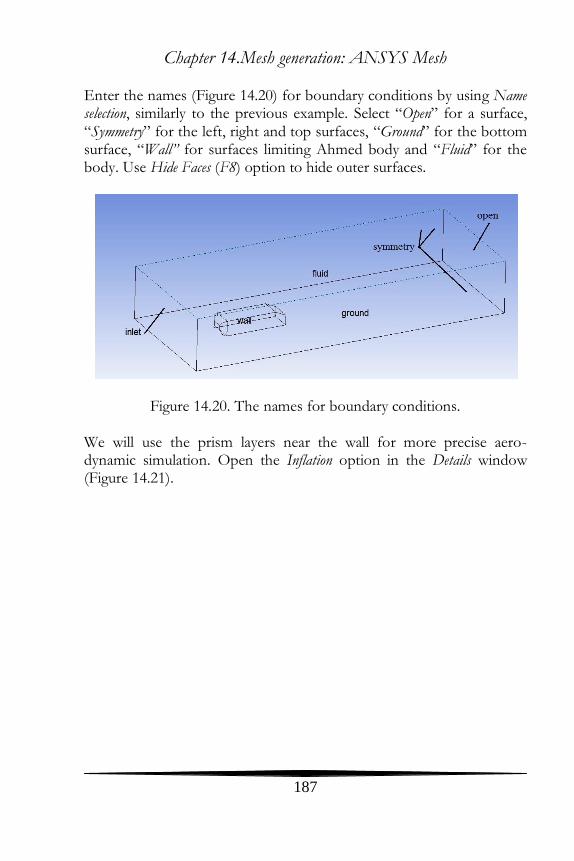
Enter the names (Figure 14.20) for boundary conditions by using Name selection, similarly to the previous example. Select “Open” for a surface, “Symmetry” for the left, right and top surfaces, “Ground” for the bottom surface, “Wall” for surfaces limiting Ahmed body and “Fluid” for the body. Use Hide Faces (F8) option to hide outer surfaces.
Figure 14.20. The names for boundary conditions. We will use the prism layers near the wall for more precise aero-dynamic simulation. Open the Inflation option in the Details window (Figure 14.21).

Chapter 14.Mesh generation: ANSYS Mesh
188
Figure 14.21. The global mesh parameters. Select Use Automatic Inflation with All Faces in Chosen Named Selection in the inflation section and specify the Wall in the Named Selection. Select First Layer Thickness in the Inflation Option, enter 1mm in the First Layer Height, and add 5 in the Maximum Layers and 1.2 in the Growth Rate. AM will generate 5 prism layers with the first 1 mm layer and the next layers will be enlarged to 1.2 times. The inflation operation in AM gives an option to generate the prism layers around chosen surfaces. After it, click on the Generate button. Change the view to Shaded exterior and Edges
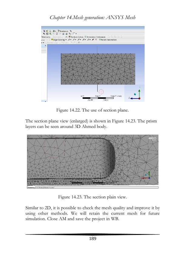
again. Now, we will see the mesh inside by creating New section plane . This option can be called from the Top toolbar. Select YZ plane and create the line that cuts the domain in vertical direction (Figure 14.22).
Chapter 14.Mesh generation: ANSYS Mesh
189
Figure 14.22. The use of section plane. The section plane view (enlarged) is shown in Figure 14.23. The prism layers can be seen around 3D Ahmed body.
Figure 14.23. The section plain view. Similar to 2D, it is possible to check the mesh quality and improve it by using other methods. We will retain the current mesh for future simulation. Close AM and save the project in WB.
Chapter 22. Acoustics
324
Chapter 22. Acoustics A simulation of noise generation plays a significant role during
development of devices from a home appliance to the gas turbine engines. The acoustic processes can not only generate a noise, but can also influence the combustion processes in engines, cause the vibrations, etc. The study of acoustic propagation and appearance is
called acoustics. Acoustics comes from Greek word ἀκουστικός (akoustikos) that means “ready to hear”.
Lighthill, a pioneer in aeroacoustics, derived a wave equation from the continuity and Navier-Stokes equations [64]. It is written as
22 22
02
ij
i i i j
Ta
t x x x x
, (22.1)
where 0a is the speed of sound and ijT is the Lighthill tensor defined
as
2
0ij i j ij ijT u u p a . (22.2)
In general, ijT represents the acoustics sources: the first source is
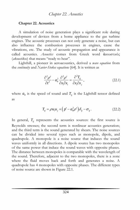
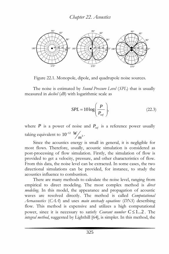
Reynolds stresses; the second term is nonlinear acoustics generation; and the third term is the sound generated by shears. The noise sources can be divided into several types such as monopole, dipole, and quadrupole. A monopole is a noise source that induces the sound waves uniformly in all directions. A dipole source has two monopoles of the same power that induce the sound waves with opposite phases. The distance between monopoles is comparable with the wavelength of the sound. Therefore, adjacent to the two monopoles, there is a zone where the fluid moves back and forth and generates a noise. A quadrupole has 4 monopoles with opposite phases. The different types of noise source are shown in Figure 22.1.
Chapter 22. Acoustics
325
Figure 22.1. Monopole, dipole, and quadrupole noise sources.
The noise is estimated by Sound Pressure Level (SPL) that is usually measured in decibel (dB) with logarithmic scale as
10logref
PSPL
P
, (22.3)
where P is a power of noise and refP is a reference power usually
taking equivalent to 1210 3W
m.
Since the acoustics energy is small in general, it is negligible for most flows. Therefore, usually, acoustic simulation is considered as post-processing of flow simulation. Firstly, the simulation of flow is provided to get a velocity, pressure, and other characteristics of flow. From this data, the noise level can be extracted. In some cases, the two directional simulations can be provided, for instance, to study the acoustics influence to combustion.
There are many methods to calculate the noise level, ranging from empirical to direct modeling. The most complex method is direct modeling. In this model, the appearance and propagation of acoustic waves are resolved directly. The method is called Computational Aeroacoustics (CAA) and uses main unsteady equations (DNS) describing flow. This method is expensive and utilizes a high computational
power, since it is necessary to satisfy Courant number 1...2C . The integral method, suggested by Lighthill [64], is simpler. In this method, the
Chapter 22. Acoustics
326
flow is first modeled by any transient simulation (DNS, LES, and URANS), and then, the data are used for the integral solution of wave equation. To obtain a model wave equation, a control surface covering the solid can be used. For the control surface, the function f is
introduced as
0,
0,
0, ,
out surface
f on surface
in surface
(22.4)
By using this function, Navier-Stokes and continuity equations, the general heterogeneous equation of Fflowcs-Williams, & Hawking [34] can be written as
2 22
2 2
0
0
1
,
ij
i j
ij j i n n
i
n n n
pp T H f
a t x x
P n u u vx
v u v ft
(22.5)
where iu is the velocity component of flow in ix direction; nu is the
velocity component normal to surface; iv is the velocity component of
surface in ix direction; nv is the velocity component of surface normal
to speed; f is Dirac delta function; 0a is the sound speed; p is
the sound pressure; and H f is the function of Heaviside defined as
1, 0
0, 0
fH f
f
(22.6)
where ijT are the components of Lighthill tensor:
Chapter 22. Acoustics
327
2
0 0ij i j ij ijT u u P a , (22.7)
and ijP is the stress tensor defined as
2
3
ji kij ij ij
j i k
uu uP p
x x x
. (22.8)
The solution of eq. (22.5) is introduced below. The detailed solution process is described in [34].
, , , ,T L Q
monopole dipole quadropole
p x t p x t p x t p x t , (22.9)
where the first source is described by
0
2
0
2
0 0
320
4 ,1
,1
n n
T
f r
n r r
f r
U Up x t dS
r M
U rM a M MdS
r M
(22.10)
the second source can be found by
2
0 0
2
2 32 200 0
14 ,
1
1,
1 1
rL
f r
r r rr M
f fr r
Lp x t dS
a r M
L rM c M ML LdS dS
ar M r M
(22.11) and the third source by
Chapter 22. Acoustics
328
2
2 2
0 0
2 3
0 0 0
14 ,
1
1 3 3.
1 1
rrQ
rf
rr ii rr ii
r rf f
Qp x t dV
a t r M
Q Q Q QdV dV
a t r M r M
(22.12) If the control surface aligns with the solid surface, the first term on the
right side of eq. 22.9, ,Tp x t represents the monopole surface source
that is defined by a solid shape and it is kinematic motion. A dipole
surface source ,Lp x t is formed by the force acting to fluid from
body. A quadruple volume source ,Qp x t is defined by the volume
sources outside of the solid body. At low speed, the last term is negligible.
In many flows, the noise does not have well-defined tones, and the acoustic energy is distributed continuously in the bright range of frequencies. In such cases, it is possible to use the turbulent statistics from the steady equations describing the flow. For example, it is sufficient to have a velocity field and the turbulent characteristics, as kinetic energy and dissipation. Such models are called the broadband models and present the semi-empirical equations that have been extracted from experiments or direct modeling. A popular model of Proudman [87] is presented below using a semi-empirical equation:
3 5
0 5
0
A
u uP a
l a
. (22.13)
For the k model , it can be re-written as
5
0
0
2A
kP a
a
, (22.14)

Chapter 22. Acoustics
329
where 0.1a is the model constant.
The main advantages, disadvantages, and limitations of acoustics models are summarized in Table 22.1.
Model Properties
CAA Excessive computational demands, reflection and scattering, transient, high accuracy
Integral High computational demands, no reflection and scattering, transient, high accuracy
Based on turbulent statistics
Low computational demands, no reflection and scattering, steady, limited accuracy
Table 22.1. Advantages, disadvantages and limitations of acoustics
models