Computational Biology, Part 12 Expression array cluster analysis Robert F. Murphy, Shann-Ching Chen...

Computational Biology, Part 12

Expression array cluster analysis

Computational Biology, Part 12

Expression array cluster analysis

Robert F. Murphy, Shann-Robert F. Murphy, Shann-Ching ChenChing Chen

Copyright Copyright 2004-2009. 2004-2009.

All rights reserved.All rights reserved.

Gene Expression MicroarrayGene Expression Microarray

A popular method to A popular method to detect mRNA expression level since reported by since reported by Pat Brown Laboratory in 1995 and by Pat Brown Laboratory in 1995 and by Affymetrix in 1996Affymetrix in 1996

Different technologies for producing Different technologies for producing the microarray chips and different the microarray chips and different approaches approaches for analyzing microarray datafor analyzing microarray data

Should carefully process and analyze Should carefully process and analyze the datathe data

What is gene expression and why is it important?

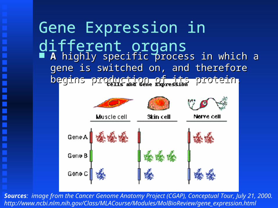
Gene Expression in different organsGene Expression in different organs AA highly specific process in which a highly specific process in which a gene is switched on, and therefore gene is switched on, and therefore begins production of its protein.begins production of its protein.

Sources: image from the Cancer Genome Anatomy Project (CGAP), Conceptual Tour, July 21, 2000. http://www.ncbi.nlm.nih.gov/Class/MLACourse/Modules/MolBioReview/gene_expression.html

Gene Expression in single organGene Expression in single organ Gene expression also varies Gene expression also varies within a certain type of cell at within a certain type of cell at different points in time. different points in time.

Sources: image from the Cancer Genome Anatomy Project (CGAP), Conceptual Tour, July 21, 2000. http://www.ncbi.nlm.nih.gov/Class/MLACourse/Modules/MolBioReview/gene_expression.html

Microarray raw dataMicroarray raw data

Label mRNA from one sample with Label mRNA from one sample with a red fluorescence probe (Cy5) a red fluorescence probe (Cy5) and mRNA from another sample and mRNA from another sample with a green fluorescence probe with a green fluorescence probe (Cy3)(Cy3)

Hybridize to a chip with Hybridize to a chip with specific DNAs fixed to each wellspecific DNAs fixed to each well

Measure amounts of green and red Measure amounts of green and red fluorescencefluorescence

Flash animations: PCR http://www.maxanim.com/genetics/PCR/PCR.htm Microarray http://www.bio.davidson.edu/Courses/genomics/chip/chip.html

Example microarray imageExample microarray image

Microarray is a technology to globally (simultaneously detecting thousands of genes) detect mRNA expression level.

mRNA expression microarray data for 9800 genes (gene number shown vertically) for 0 to 24 h (time shown horizontally) after addition of serum to a human cell line that had been deprived of serum (from http://genome-www.stanford.edu/serum)

Data extractionData extraction

Adjust fluorescent intensities Adjust fluorescent intensities using standards (as necessary)using standards (as necessary)

Calculate ratio of red to green Calculate ratio of red to green fluorescencefluorescence

Convert to logConvert to log22 and round to and round to integer integer

Display saturated green=-3 to Display saturated green=-3 to black = 0 to saturated red = +3black = 0 to saturated red = +3

Many different types:• Hierarchical clustering • k – means clustering• Self-organising maps

• Hill Climbing

• Simulated Annealing

All have the same three basic tasks of:

1. Pattern representation – patterns or features in the data.2. Pattern proximity – a measure of the distance or

similarity defined on pairs of patterns3. Pattern grouping – methods and rules used in grouping

the patterns

Unsupervised clustering algorithms

DistancesDistances

High High dimensionalitydimensionality

Based on Based on vector vector geometrygeometry – how – how close are two close are two data points?data points?

Array2

Array 1

Array 1 Array 2

Gene 1 1 4

…

Gene 1

DistancesDistances



Array2

Array 1

Array 1 Array 2

Gene 1 1 4

Gene 2 1 3

…

Gene 1Gene 2

Distance(Gene 1, Gene 2) = 1

DistancesDistances



Based on Based on distances to distances to determine determine clustersclusters

Array2

Array 1

Array 1 Array 2

Gene 1 1 4

Gene 2 1 3

…

Gene 1Gene 2

Distance(Gene 1, Gene 2) = 1

a1

a2 b2

b1

Distance

Sample 2

Sample 1

Gene aGene b

sample 1 sample 2

a1 a2b1 b2

Bivariate Euclidean Distance

General Multivariate DatasetGeneral Multivariate Dataset We are given values of We are given values of pp variables for variables for nn independent independent observationsobservations

Construct an Construct an n n xx p p matrix matrix MM consisting of vectors consisting of vectors XX11 through through XXnn each of length each of length pp

Multivariate Sample MeanMultivariate Sample Mean Define mean vector Define mean vector II of of length length pp

I( j) =M(i, j)

i=1

n∑

nI =

Xii=1

n∑

nor

matrix notation vector notation

Multivariate VarianceMultivariate Variance

Define variance vector Define variance vector of of length length pp

σ 2( j) =M(i, j)−I( j)( )

i=1

n∑

2

n−1matrix notation

Multivariate VarianceMultivariate Variance

oror

σ 2 =Xi −I( )

i=1

n∑

2

n−1vector notation

Covariance MatrixCovariance Matrix

Define a Define a p p x x p p matrix matrix covcov (called the (called the covariance matrixcovariance matrix) analogous to ) analogous to 22

cov( j,k) =M(i, j)−I(j)( )M(i,k)−I(k)( )

i=1

n∑

n−1

Covariance MatrixCovariance Matrix

Note that the covariance of a variable with Note that the covariance of a variable with itself is simply the variance of that itself is simply the variance of that variablevariable

cov( j, j) =σ 2( j)

Univariate DistanceUnivariate Distance

The simple distance between the values of a The simple distance between the values of a single variable single variable jj for two observations for two observations ii and and ll is is

M(i, j)−M(l, j)

Univariate z-score DistanceUnivariate z-score Distance

To measure distance To measure distance in units of in units of standard deviation standard deviation between the between the values of a single variable values of a single variable jj for for two observations two observations ii and and ll we define we define the the z-score distancez-score distance

M(i, j)−M(l, j)σ( j)

Bivariate Euclidean DistanceBivariate Euclidean Distance The most commonly used measure of distance The most commonly used measure of distance between two observations between two observations ii and and ll on two on two variables variables jj and and k k is the is the Euclidean distanceEuclidean distance

M(i, j)−M(l, j)( )2 + M(i,k)−M(l,k)( )2

M(i,j)

k variable

j variable

i observation

l observationM(l,j)

M(i,k) M(l,k)

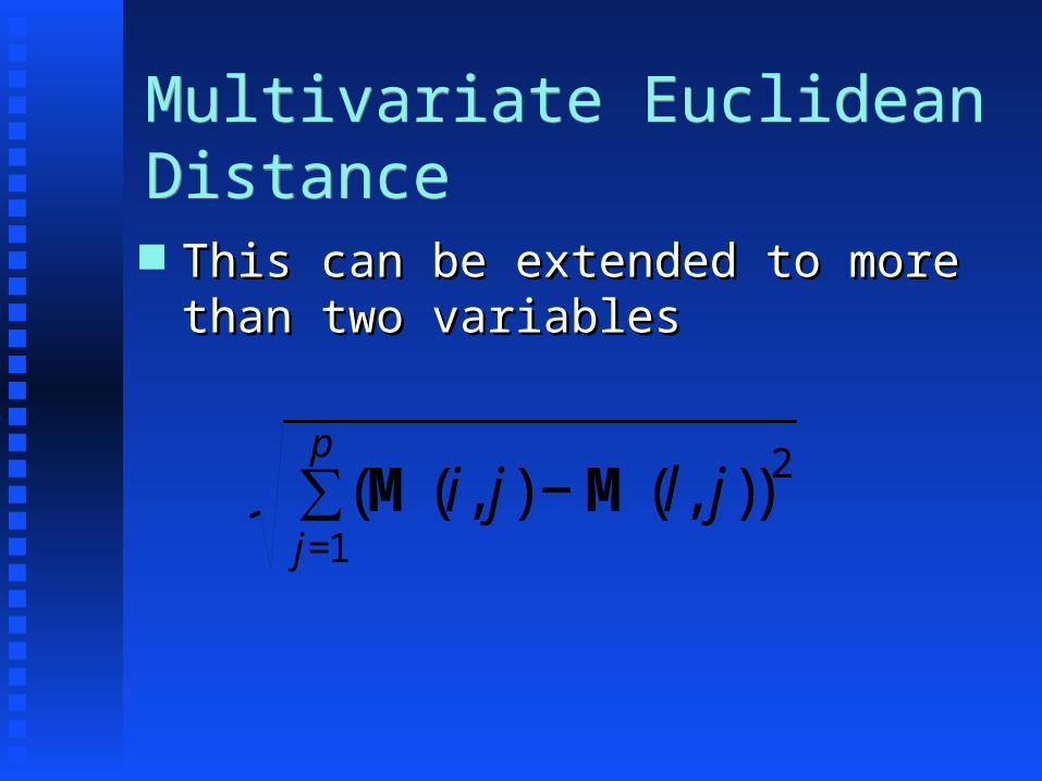
Multivariate Euclidean DistanceMultivariate Euclidean Distance This can be extended to more This can be extended to more than two variablesthan two variables

M(i, j)−M(l, j)( )2j=1

p∑

Effects of variance and covariance on Euclidean distance

Effects of variance and covariance on Euclidean distance

Points A and B have similar Euclidean distances from the mean, but point B is clearly “more different” from the population than point A.

BA

The ellipse shows the 50% contour of a hypothetical population.

Mahalanobis DistanceMahalanobis Distance

To account for differences in To account for differences in variance between the variables, and variance between the variables, and to account for correlations between to account for correlations between variables, we use the variables, we use the Mahalanobis Mahalanobis distancedistance

D2 = Xi −Xl( )cov-1 Xi −Xl( )T

Other distance functionsOther distance functions We can use other distance We can use other distance functions, including ones in functions, including ones in which the weights on each which the weights on each variable are learnedvariable are learned

Cluster analysis tools for Cluster analysis tools for microarray data most commonly microarray data most commonly use Pearson correlation use Pearson correlation coefficientcoefficient

Pearson correlation coefficientPearson correlation coefficient

€

S(X,Y ) =1/N (i=1

N

∑X i − Xoffset

ΦX

)(Yi −Yoffset

ΦY

)

ΦX =(X i − Xoffset )

2

Ni=1

N

∑ ΦY =(Yi −Yoffset )

2

Ni=1

N

∑

Software for performing microarray cluster analysis

Software for performing microarray cluster analysis http://rana.lbl.gov/EisenSoftware.htm

Michael Eisen’s Cluster (Windows Michael Eisen’s Cluster (Windows only)only)

M. de Hoon’s Cluster 3.0 (all OS)M. de Hoon’s Cluster 3.0 (all OS) Tree viewing (links on same site)Tree viewing (links on same site)

Java TreeviewJava Treeview MapletreeMapletree

Input data for clusteringInput data for clustering Genes in rows, conditions in Genes in rows, conditions in columnscolumnsYORF NAME GWEIGHT Cell-cycle Alpha-Factor 1Cell-cycle Alpha-Factor 2Cell-cycle Alpha-Factor 3

EWEIGHT 1 1 1YHR051W YHR051W COX6 oxidative phosphorylation cytochrome-c oxidase subunit VI S00010931 0.03 0.3 0.37YKL181W YKL181W PRS1 purine, pyrimidine, tryptophanphosphoribosylpyrophosphate synthetase S00016641 0.33 -0.2 -0.12YHR124W YHR124W NDT80 meiosis transcription factor S00011661 0.36 0.08 0.06YHL020C YHL020C OPI1 phospholipid metabolism negative regulator of phospholipid biosynthesS00010121 -0.01 -0.03 0.21YGR072W YGR072W UPF3 mRNA decay, nonsense-mediated unknown S00033041 0.2 -0.43 -0.22YGR145W YGR145W unknown unknown; similar to MESA gene of Plasmodium fS00033771 0.11 -1.15 -1.03YGR218W YGR218W CRM1 nuclear protein targeting nuclear export factor S00034501 0.24 -0.23 0.12YGL041C YGL041C unknown unknown S00030091 0.06 0.23 0.2YOR202W YOR202W HIS3 histidine biosynthesis imidazoleglycerol-phosphate dehydratase S00057281 0.1 0.48 0.86YCR005C YCR005C CIT2 glyoxylate cycle peroxisomal citrate synthase S00005981 0.34 1.46 1.23YER187W YER187W unknown unknown; similar to killer toxin Khs1p S00009891 0.71 0.03 0.11YBR026C YBR026C MRF1' mitochondrial respiration ARS-binding protein S00002301 -0.22 0.14 0.14YMR244W YMR244W unknown unknown; similar to Nca3p S00048581 0.16 -0.18 -0.38YAR047C YAR047C unknown unknown S00000831 -0.43 -0.56 -0.14YMR317W YMR317W unknown unknown S00049361 -0.43 -0.03 0.21

An Introduction to Bioinformatics Algorithms

www.bioalgorithms.info

Clustering of Microarray Data (cont’d)

Clusters



Homogeneity and Separation Principles• Homogeneity: Elements within a cluster are close

to each other• Separation: Elements in different clusters are

further apart from each other• …clustering is not an easy task!

Given these points a clustering algorithm might make two distinct clusters as follows



Bad Clustering

This clustering violates both Homogeneity and Separation principles

Close distances from points in separate clustersFar distances

from points in the same cluster



Good Clustering

This clustering satisfies both Homogeneity and Separation principles



Clustering Techniques

• Agglomerative: Start with every element in its own cluster, and iteratively join clusters together

• Divisive: Start with one cluster and iteratively divide it into smaller clusters

• Hierarchical: Organize elements into a tree, leaves represent genes and the length of the pathes between leaves represents the distances between genes. Similar genes lie within the same subtrees



Hierarchical Clustering



Hierarchical Clustering: Example



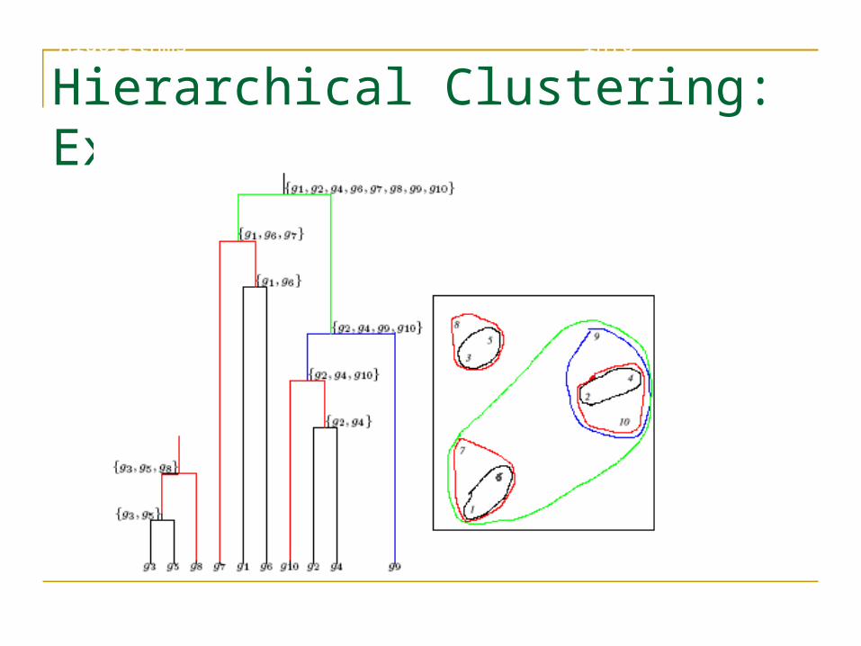
Hierarchical Clustering (cont’d)• Hierarchical Clustering is often used to reveal

evolutionary history



Hierarchical Clustering Algorithm1. Hierarchical Clustering (d , n)2. Form n clusters each with one element3. Construct a graph T by assigning one vertex to

each cluster4. while there is more than one cluster5. Find the two closest clusters C1 and C2

6. Merge C1 and C2 into new cluster C with |C1| +|C2| elements

7. Compute distance from C to all other clusters8. Add a new vertex C to T and connect to vertices

C1 and C2

9. Remove rows and columns of d corresponding to C1 and C2

10. Add a row and column to d corrsponding to the new cluster C

11. return T

The algorithm takes a nxn distance matrix d of pairwise distances between points as an input.



Hierarchical Clustering Algorithm1. Hierarchical Clustering (d , n)2. Form n clusters each with one element3. Construct a graph T by assigning one vertex to each

cluster4. while there is more than one cluster5. Find the two closest clusters C1 and C2

6. Merge C1 and C2 into new cluster C with |C1| +|C2| elements

7. Compute distance from C to all other clusters8. Add a new vertex C to T and connect to vertices C1 and

C2

9. Remove rows and columns of d corresponding to C1 and C2

10. Add a row and column to d corrsponding to the new cluster C

11. return T

Different ways to define distances between clusters may lead to different clusterings



Hierarchical Clustering: Recomputing Distances

• dmin(C, C*) = min d(x,y) for all elements x in C and y in C*

• Distance between two clusters is the smallest distance between any pair of their elements

• davg(C, C*) = (1 / |C*||C|) ∑ d(x,y) for all elements x in C and y in C*

• Distance between two clusters is the average distance between all pairs of their elements



Squared Error Distortion• Given a data point v and a set of points X, define the distance from v to X

d(v, X)

as the (Eucledian) distance from v to the closest point from X.

• Given a set of n data points V={v1…vn} and a set of k points X, define the Squared Error Distortion

d(V,X) = ∑d(vi, X)2 / n 1 < i < n



K-Means Clustering Problem: Formulation• Input: A set, V, consisting of n points and a

parameter k

• Output: A set X consisting of k points (cluster centers) that minimizes the squared error distortion d(V,X) over all possible choices of X



1-Means Clustering Problem: an Easy Case• Input: A set, V, consisting of n points

• Output: A single points x (cluster center) that minimizes the squared error distortion d(V,x) over all possible choices of x



1-Means Clustering Problem: an Easy Case• Input: A set, V, consisting of n points

• Output: A single points x (cluster center) that minimizes the squared error distortion d(V,x) over all possible choices of x

1-Means Clustering problem is easy.

However, it becomes very difficult (NP-complete) for more than one center.

An efficient heuristic method for K-Means clustering is the Lloyd algorithm



K-Means Clustering: Lloyd Algorithm1. Lloyd Algorithm2. Arbitrarily assign the k cluster centers3. while the cluster centers keep changing4. Assign each data point to the cluster Ci

corresponding to the closest cluster representative (center) (1 ≤ i ≤ k)

5. After the assignment of all data points, compute new cluster representatives according to the center of gravity of each cluster, that is, the new cluster representative is ∑v \ |C| for all v in C for

every cluster C

*This may lead to merely a locally optimal clustering.



0

1

2

3

4

5

0 1 2 3 4 5

expression in condition 1

exp

ressio

n in

co

nd

itio

n 2

x1

x2

x3



0

1

2

3

4

5

0 1 2 3 4 5


exp

ress

ion

in c

on

dit

ion

2

x1

x2

x3



0

1

2

3

4

5

0 1 2 3 4 5


exp

ress

ion

in c

on

dit

ion

2

x1

x2 x3



Clique Graphs

• A clique is a graph with every vertex connected to every other vertex

• A clique graph is a graph where each connected component is a clique



Transforming an Arbitrary Graph into a Clique Graphs

• A graph can be transformed into a clique graph by adding or removing edges



Corrupted Cliques Problem

Input: A graph G

Output: The smallest number of additions and removals of edges that will transform G into a clique graph



Distance Graphs

• Turn the distance matrix into a distance graph

• Genes are represented as vertices in the graph

• Choose a distance threshold θ

• If the distance between two vertices is below θ, draw an edge between them

• The resulting graph may contain cliques

• These cliques represent clusters of closely located data points!



Transforming Distance Graph into Clique Graph

The distance graph (threshold θ=7) is transformed into a clique graph after removing the two highlighted edges

After transforming the distance graph into the clique graph, the dataset is partitioned into three clusters



Heuristics for Corrupted Clique Problem• Corrupted Cliques problem is NP-Hard, some heuristics

exist to approximately solve it:• CAST (Cluster Affinity Search Technique): a practical and

fast algorithm:• CAST is based on the notion of genes close to cluster

C or distant from cluster C• Distance between gene i and cluster C: d(i,C) = average distance between gene i and all genes in C

Gene i is close to cluster C if d(i,C)< θ and distant otherwise



CAST Algorithm1. CAST(S, G, θ)2. P Ø3. while S ≠ Ø4. V vertex of maximal degree in the distance graph G5. C {v}6. while a close gene i not in C or distant gene i in C

exists7. Find the nearest close gene i not in C and add it

to C8. Remove the farthest distant gene i in C9. Add cluster C to partition P10. S S \ C11. Remove vertices of cluster C from the distance graph G12. return P

S – set of elements, G – distance graph, θ - distance threshold

Choosing the number of CentersChoosing the number of Centers A difficult problemA difficult problem Most common approach is to try to Most common approach is to try to find thefind thesolution that minimizes the Bayesian solution that minimizes the Bayesian Information CriterionInformation Criterion

2ln ln( )BIC L k n=− +L = the

likelihood function for the estimated

model

K = # of parameters

n = # of samples

Clustering genes and conditionsClustering genes and conditions

Rows and Rows and columns can be columns can be clustered clustered independently independently - hierarchical - hierarchical is preferred is preferred for for visualizing visualizing thisthis

Computational Biology, Part 12 Expression array cluster analysis Robert F. Murphy, Shann-Ching Chen...

Documents

Transcript of Computational Biology, Part 12 Expression array cluster analysis Robert F. Murphy, Shann-Ching Chen...