Computation of Scattering Clusters of Spheres Using the Fast Multipole Method

Nail A. Gumerov Ramani Duraiswami

Institute for Advanced Computer StudiesUniversity of Maryland at College Parkwww.umiacs.umd.edu/~gumerovwww.umiacs.umd.edu/~ramaniThis study has been supported by NSF

Outline

IntroductionProblem FormulationMethod of Solution

Multipole Reexpansion (T-matrix) MethodIterative MethodsFast Multipole Method

Results of ComputationsConclusion

Introduction

Multiple Scattering Problems

Sound propagation in disperse media (particles, bubbles, etc.)

Modeling of scattering from environment (humans, animals, fish, etc.)

Electromagnetic scattering problems (microwaves, optics, etc.)

Efficient parametrization in inverse problems (tomography, etc.)

Introduction

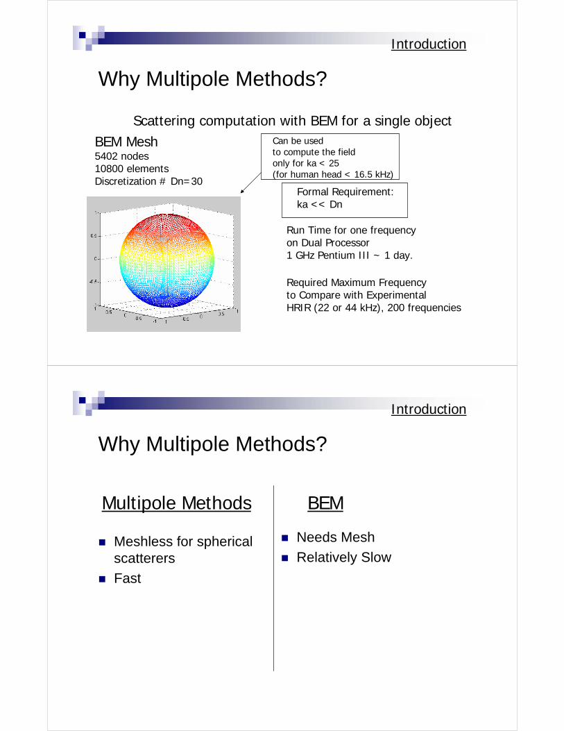
Why Multipole Methods?

Introduction

BEM Mesh5402 nodes10800 elementsDiscretization # Dn=30

Can be usedto compute the fieldonly for ka < 25 (for human head < 16.5 kHz)

Run Time for one frequencyon Dual Processor1 GHz Pentium III ~ 1 day.

Required Maximum Frequency to Compare with ExperimentalHRIR (22 or 44 kHz), 200 frequencies

Formal Requirement:ka << Dn

Scattering computation with BEM for a single object

Why Multipole Methods?

Meshless for spherical scatterers

Fast

Needs Mesh

Relatively Slow

Introduction

Multipole Methods BEM

Problem Formulation

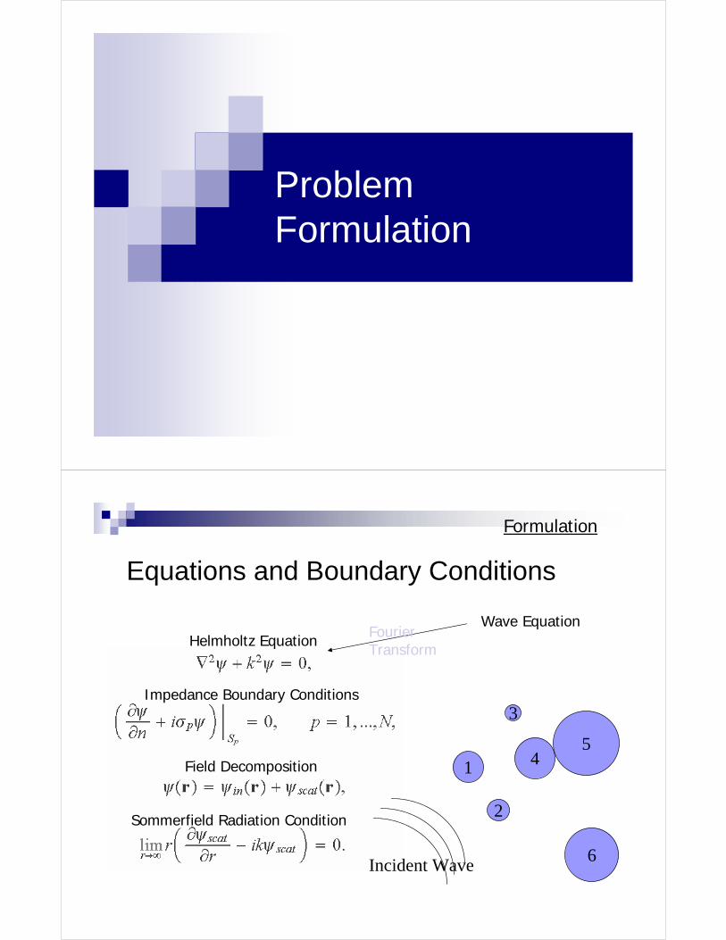
Equations and Boundary Conditions

Helmholtz Equation

Impedance Boundary Conditions

Field Decomposition

Sommerfield Radiation Condition

4

2

1

6

5

3

Incident Wave

Formulation

Wave EquationFourierTransform

Multipole Reexpansion(T-Matrix) Method

Scattered Field Decomposition

T-Matrix Method

Expansion Coefficients

Singular Basis Functions Hankel Functions

Spherical Harmonics

Vector Form:

dot product

Incident Field Decompositionand T-matrix for a Single Sphere

T-Matrix Method

Regular Basis Functions Bessel Functions

Analytical Solution of the Problem:

T-matrix

Isosurfaces For Regular Basis Functions

n

m

Isosurfaces For Singular Basis Functions

n

m

Solution of Multiple Scattering Problem

T-Matrix Method

4

2

1

6

5

3

Incident Wave

Scattered Wave

Coupled System of Equations:

(S|R)-TranslationMatrix

“Effective” Incident Field

Reexpansions/Translations

T-Matrix Method

q

p

M

O

rp

rq

r’pr’q

r’pq

r q

p

M

O

rp

rq

r’pr’q

r’pq

r

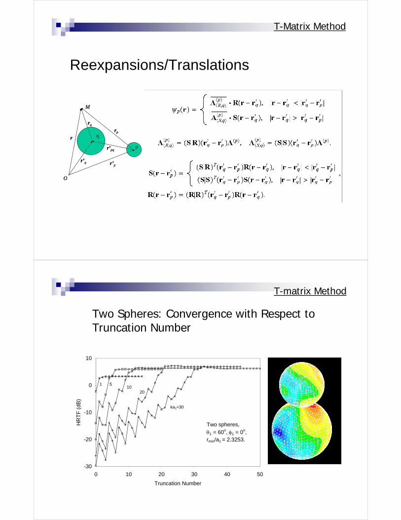
Two Spheres: Convergence with Respect to Truncation Number

T-matrix Method

-30

-20

-10

0

10

0 10 20 30 40 50

Truncation Number

HR

TF

(dB

)

ka1=30

5110

20

Two spheres,

θ1 = 60o, φ1 = 0o,rmin/a1 = 2.3253.

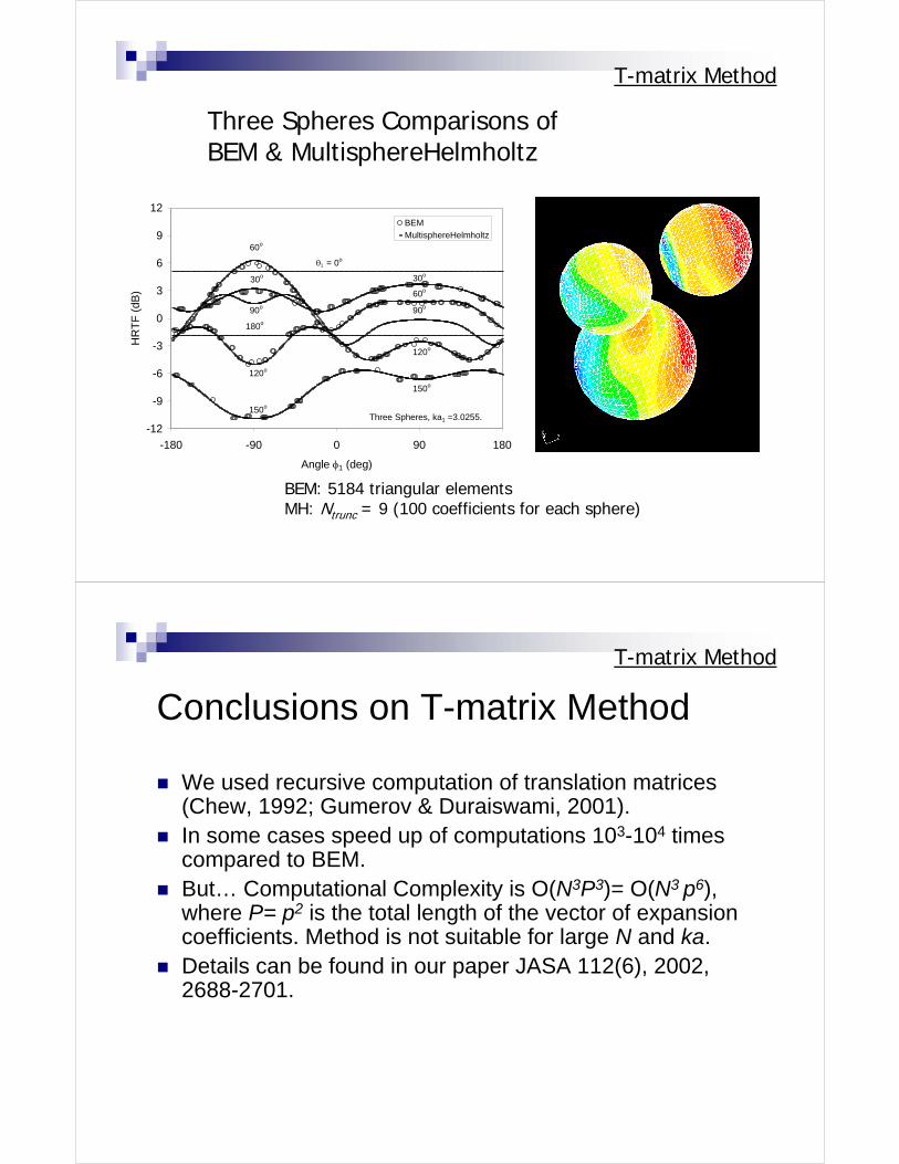
Three Spheres Comparisons ofBEM & MultisphereHelmholtz

T-matrix Method

BEM: 5184 triangular elementsMH: Ntrunc = 9 (100 coefficients for each sphere)

-12

-9

-6

-3

0

3

6

9

12

-180 -90 0 90 180

Angle φ1 (deg)

HR

TF

(dB

)

BEM

MultisphereHelmholtz

θ1 = 0o

30o

60o

90o

60o

30o

90o

120o

120o

150o

150o

180o

Three Spheres, ka1 =3.0255.

Conclusions on T-matrix Method

We used recursive computation of translation matrices (Chew, 1992; Gumerov & Duraiswami, 2001). In some cases speed up of computations 103-104 times compared to BEM.But… Computational Complexity is O(N3P3)= O(N3 p6), where P= p2 is the total length of the vector of expansion coefficients. Method is not suitable for large N and ka.Details can be found in our paper JASA 112(6), 2002, 2688-2701.

T-matrix Method

Iterative Methods

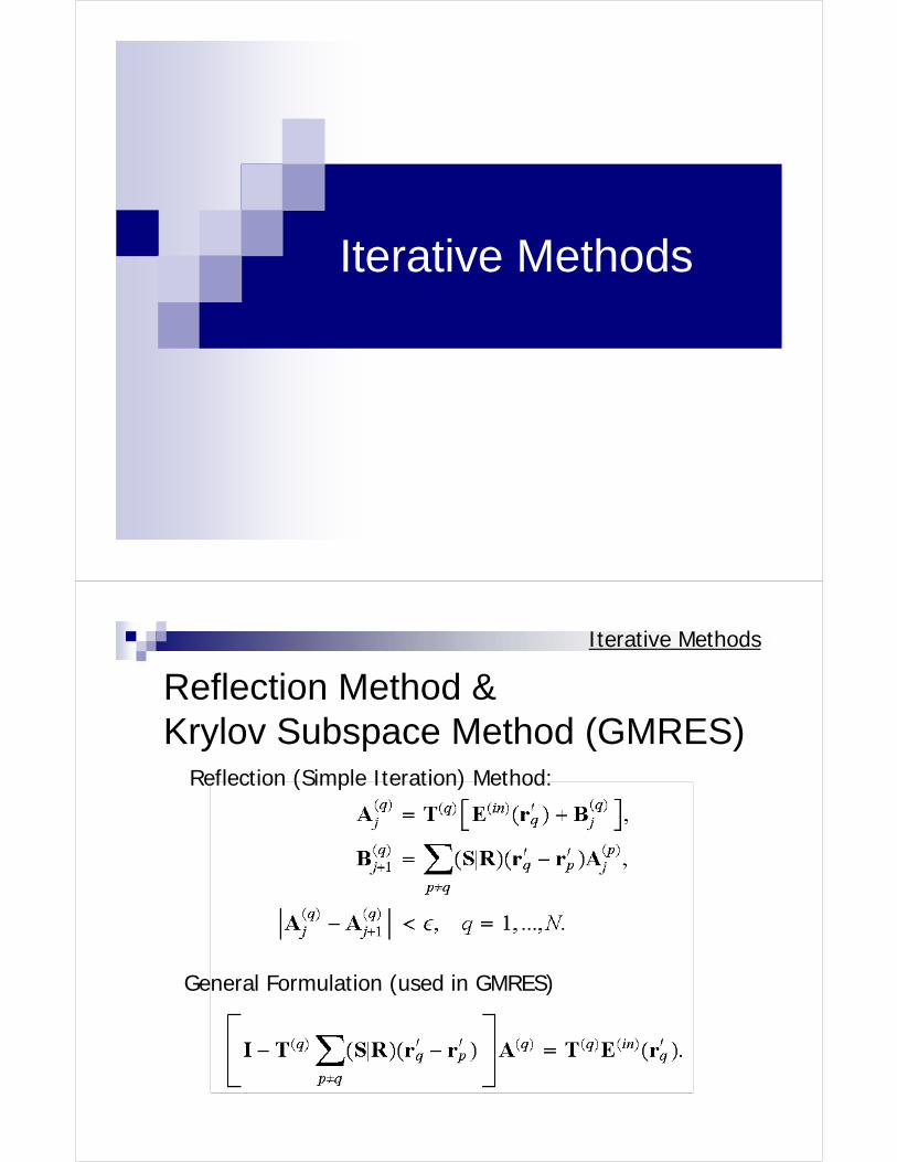
Reflection Method & Krylov Subspace Method (GMRES)

Reflection (Simple Iteration) Method:

General Formulation (used in GMRES)

Iterative Methods

Convergence of Reflection Iteration Method

Iterative Methods

Exponential Convergence

Conclusions on Iterative Methods

Both the Reflection Method (RM) and the GMRES converge well, while the RM is simpler and faster;Some problems in convergence were found for larger ka and regular spacing of the scatterers;In iterative methods fast translation algorithms can be used (weused O(p3)=O(P3/2) fast translation based on sparse matrix decomposition of translation operators). This cost potentially can be reduced further (we are working on O(PlogP) methods).Complexity of Iterative Methods in this case O(N2Niter p3); Savings in complexity compared to straightforward T-matrix are O(p3

N/Niter)For N~200, Niter~20, p~10 (P~100) this yields of order 104 times savings.

Iterative Methods

Fast Multipole Method

Some Facts on the Fast Multipole Methods (FMM)

Introduced by Rokhlin & Greengard (1987,1988) for computation of 2D and 3D fields for Laplace Equation;Reduces complexity of matrix-vector product from O(N2) to O(N)or O(NlogN) (depends on data structure);Hundreds of publications for various 1D, 2D, and 3D problems (Laplace, Helmholtz, Maxwell, Yukawa Potentials, etc.);Application to acoustical scattering problems (Koc & Chew, 1998; JASA);We taught the first in the country course on FMM fundamentals & application at the University of Maryland (2002,2003);Some technical reports are available online;A book on the FMM for the 3D Helmholtz equation submitted to Academic Press.

FMM

Far and Near FieldsFMM

Neighborhood(Near Field)

Far Field

Max Level of Space Subdivision

Translations

Ω1

Ω2

x*1

x*2R (R|R)

x R

Ωr(x*)

x*

(R|R)

y x*+tt

r

Ωr1(x*+t)

r1

xi

Ω1

Ω2x*1

x*2

S

(S|S)

S

xi

x*x*+t

(S|S)

y

t

Ωr1(x*+t) Ωr(x*)

rr1

xi

Ω1

x*1x*2

S

(S|S)

S

xi

x*

x*+t

(S|R)

y

t

Ωr1(x*+t)

r

r1

R|R S|S S|R

FMM

Problem:For the Helmholtz equation absolute and uniform convergence can be achieved only for

p > ka. For large ka the FMM with constant p isvery expensive (comparable with straightforward methods);

inaccurate (since keeps much larger number of terms than required, which causes numerical instabilities).

a

ExpansionDomain

D

2a=31/2D

Model of Truncation Number Behavior for Fixed Error

p

ka0 ka*

p*

In the multilevel FMM we associate its own pl

with each level l:

“Breakdown level”

Box size at level l

Complexity of Single Translation

Translation exponent

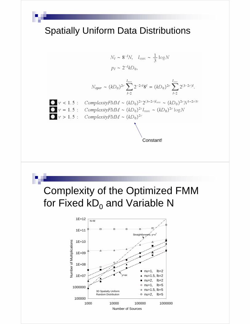
Spatially Uniform Data Distributions

Constant!

Complexity of the Optimized FMM for Fixed kD0 and Variable N

100000

1000000

1E+07

1E+08

1E+09

1E+10

1E+11

1E+12

1000 10000 100000 1000000

Number of Sources

Num

ber

of

Mul

tiplic

atio

ns

nu=1, lb=2nu=1.5, lb=2nu=2, lb=2nu=1, lb=5nu=1.5, lb=5nu=2, lb=5

Straightforward, y=x2

3D Spatially Uniform Random Distribution

N=M

y=ax

Optimum Level for Low Frequencies

0.00001

0.0001

0.001

0.01

0.1

1

10

100

2 3 4 5 6 7

Max Level of Space Subdivision

Num

ber

of M

ultip

licat

ions

, x10

e11

N=M=10000003D Spatially Uniform Random Distribution

Direct Summation

Translation

Total

nu=1

1.5

2

2

1.5

1

Volume Element Methods

Ns

wavelength

D0 = D0 k/(2π) wavelengths = N1/3 sourcesCritical Translation Exponent!

computational domain

What Happens if Truncation Number is Constant for All Levels?

“Catastrophic Disaster of the FMM”

Source Expansion Errors

rs

r

ab

rs

r

ab0 0

rs

r

ab

rs

r

ab0 0

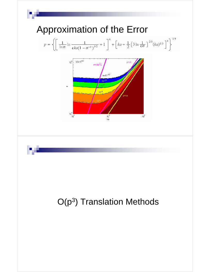
Approximation of the Error

O(p3) Translation Methods

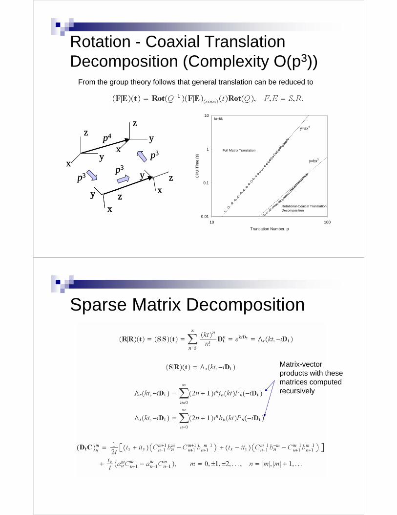
Rotation - Coaxial Translation Decomposition (Complexity O(p3))

z

y

y

x

x

y

xz

y

xz

z

p4

p3p3

p3

z

y

y

x

x

y

xzy

xz

y

xz

z

p4

p3p3

p3

From the group theory follows that general translation can be reduced to

0.01

0.1

1

10

10 100

Truncation Number, p

CP

U T

ime

(s)

Full Matrix Translation

Rotational-Coaxial Translation Decomposition

y=ax4

y=bx3

kt=86

Sparse Matrix Decomposition

Matrix-vector products with these matrices computed recursively

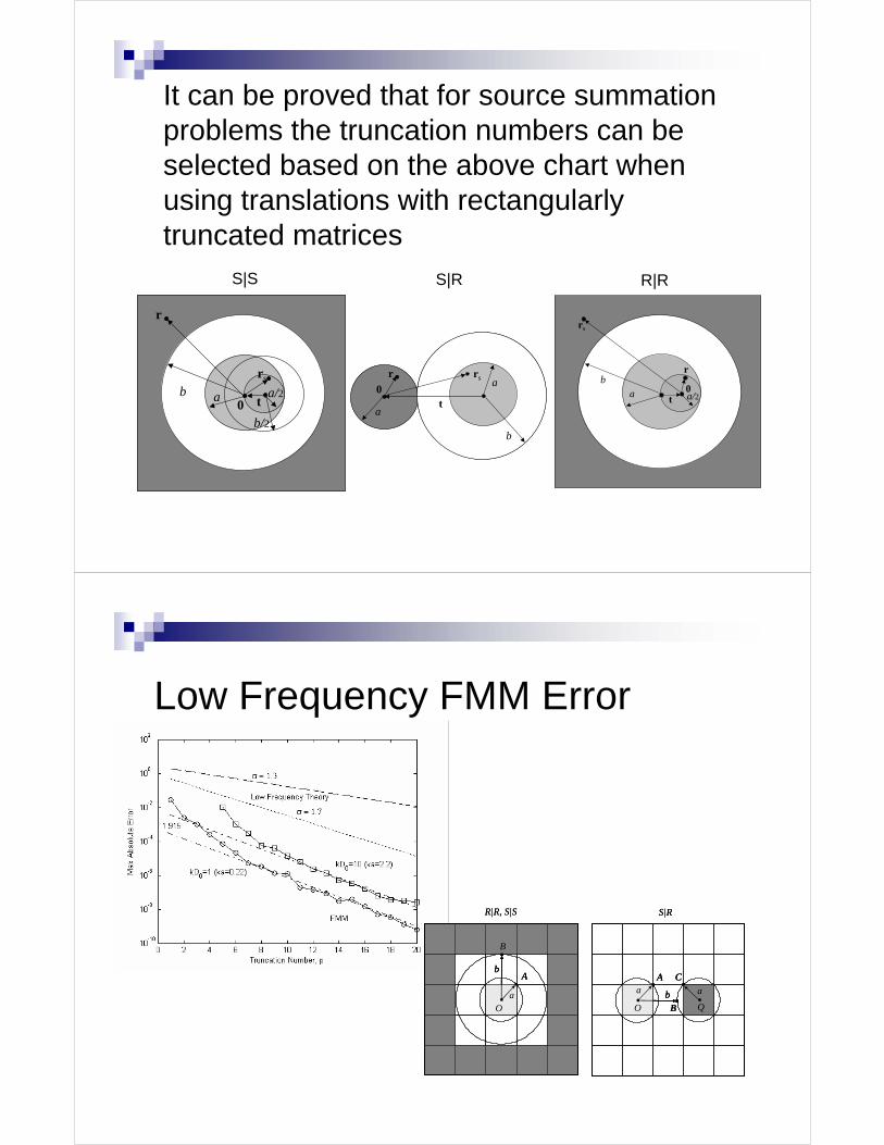
It can be proved that for source summation problems the truncation numbers can be selected based on the above chart when using translations with rectangularlytruncated matrices

r

ab0

rs

a/2t

b/2

r

ab0

rs

a/2t

b/2

ra

b

0

rs

ta

ra

b

0

rs

ta

r

ab

rs

a/2t0

r

ab

rs

a/2t0

S|S S|R R|R

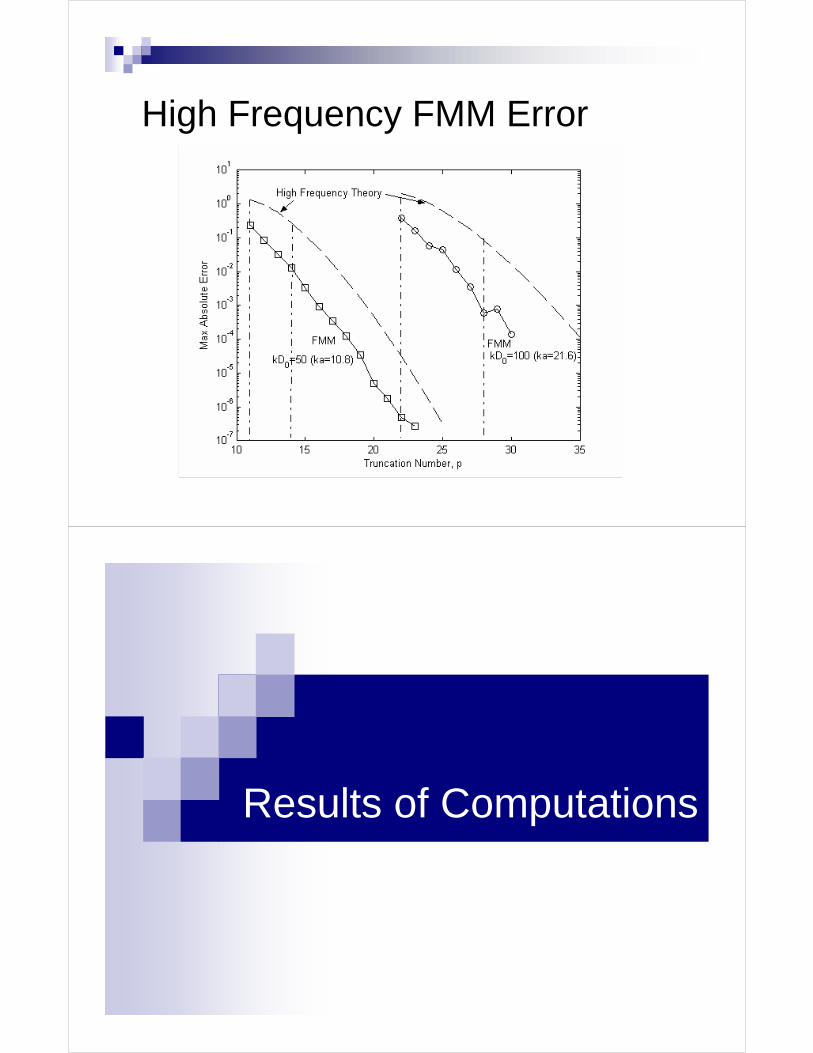
Low Frequency FMM Error

a

b

O

A

B

ab

C

B

a

O

A

Q

R|R, S|S S|R

a

b

O

A

B

ab

C

B

a

O

A

Qa

b

O

A

B

ab

C

B

a

O

A

Q

R|R, S|S S|R

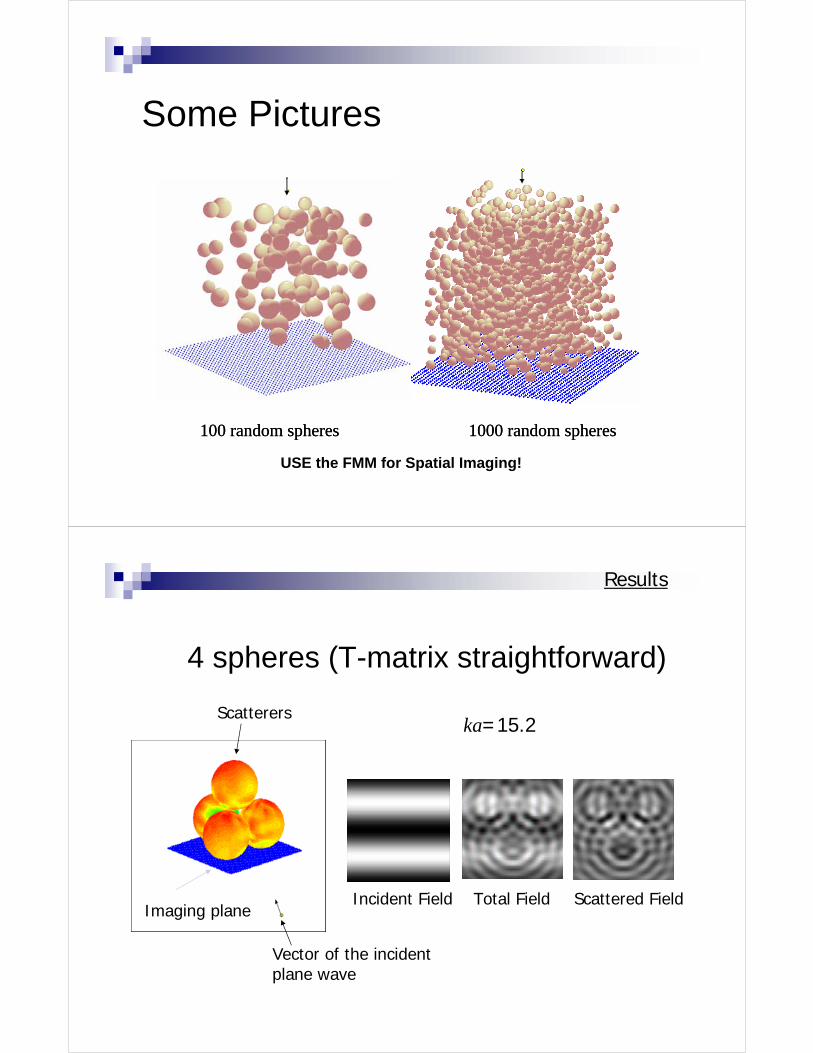
High Frequency FMM Error

Results of Computations

Range of Parameters

Number of Spheres: 1-104;

ka: 0.1-10; kD0: 1-100;

Random and regularly spaced grids of spheres;

Polydispersity: 0.5-1.5 (ratio to the mean radius);

Volume fractions: 0.01-0.2;

Results

Advantages and Defficiencies of Our FMM Implementation

O(NlogN) “On fly” computation of neighbor lists, using bit interleaving;

Low memory: one can trade memory for speed;Rotation-Coaxial Translation Decomposition, Operations with Multipole Expansion Coefficients;

For high frequencies some other methods (diagonal forms, asymptotic methods) can be used; Some additional complexity: conversion to the space of expansion coefficients;

No precomputation of translation and rotation matrices; Low memory: one can trade memory for speed;

For larger problem size the GMRES is more efficient than the Reflection Method;

User can switch, but the GMRES can be used as default.Krylov subspace dimensionalities usually low (of order 10-30).

This implementation is not perfect, but works!

Some Configurations

343 640 1000343 640 1000

Surface Potential Imaging

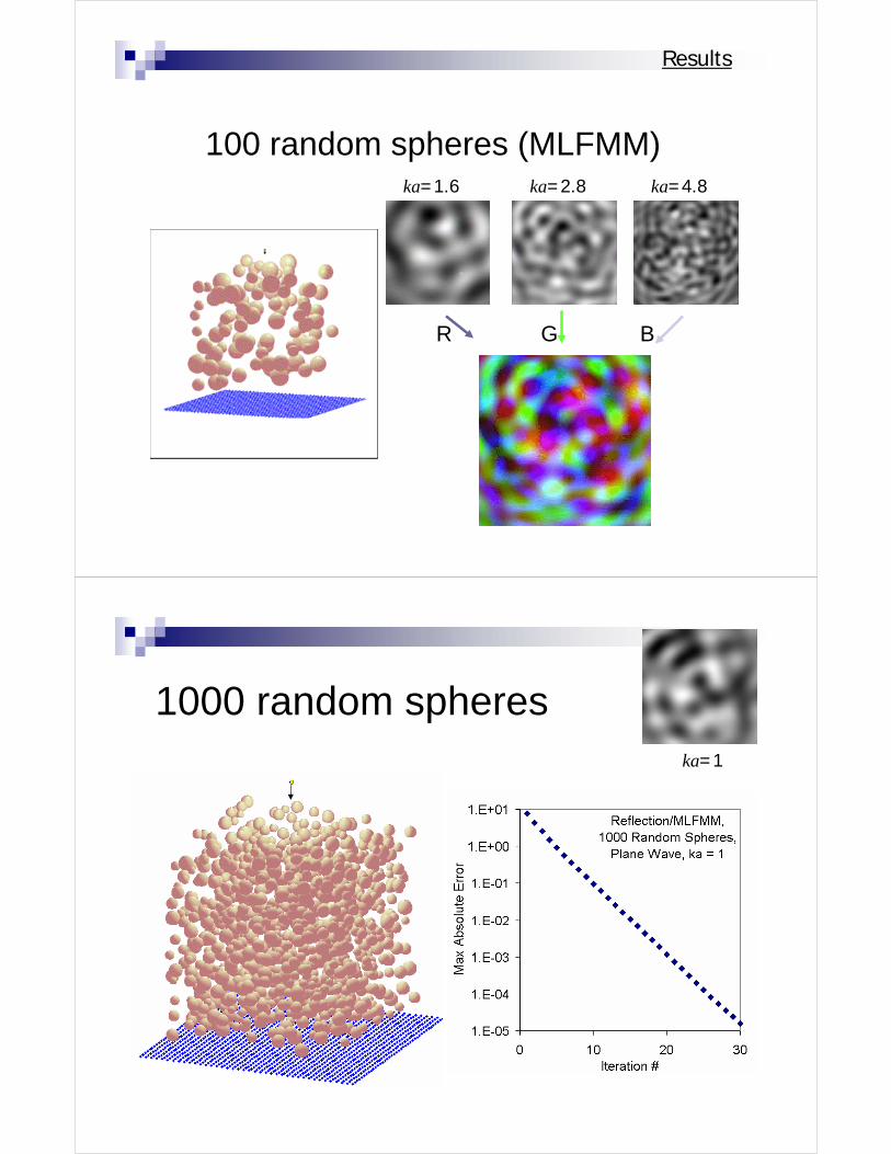
Some Pictures

100 random spheres 1000 random spheres100 random spheres 1000 random spheres

USE the FMM for Spatial Imaging!

4 spheres (T-matrix straightforward)

Results

Vector of the incidentplane wave

Imaging plane

Scattererska=15.2

Incident Field Total Field Scattered Field

100 random spheres (MLFMM)

Results

ka=1.6 ka=4.8ka=2.8

R G B

1000 random sphereska=1

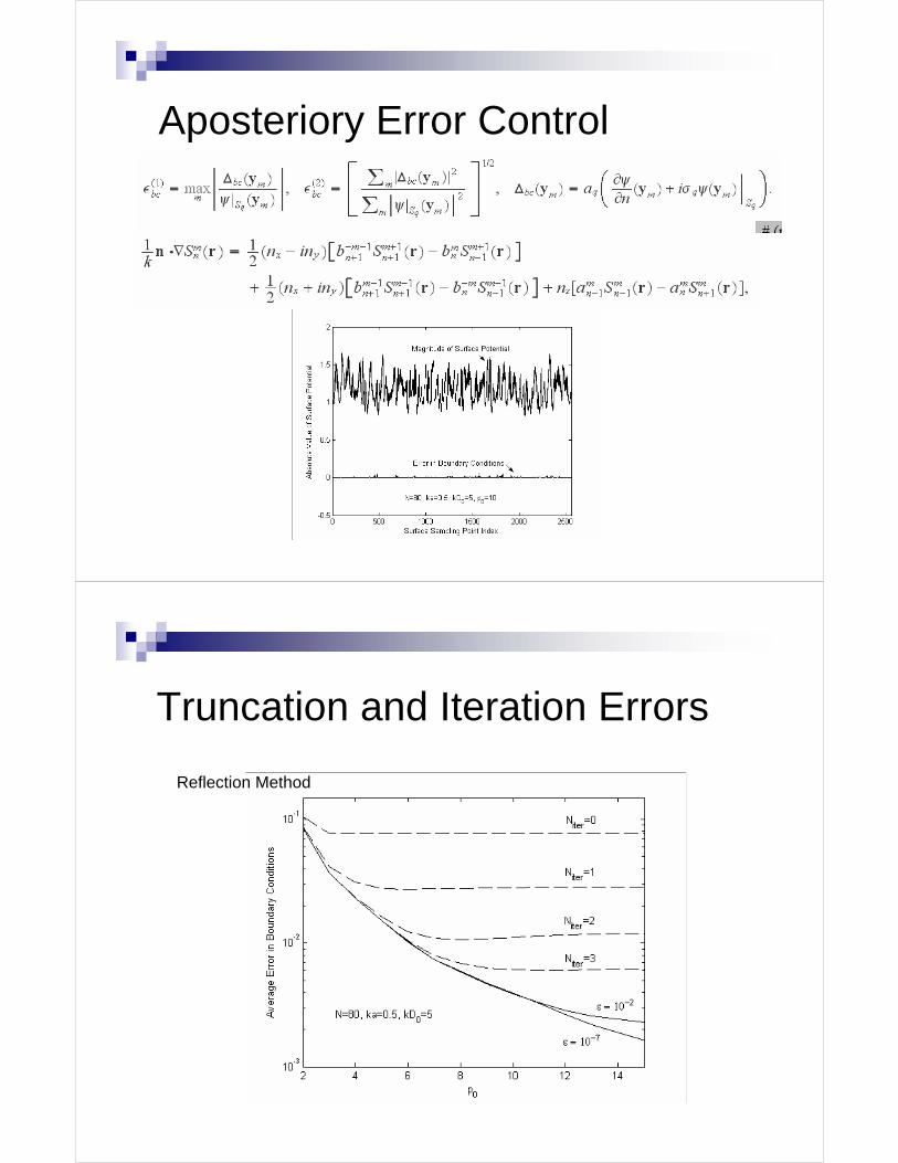
Aposteriory Error Control

Truncation and Iteration Errors

Reflection Method

Convergence for 100 spheres (MLFMM)

Results

1.E-04

1.E-03

1.E-02

1.E-01

1.E+00

1.E+01

1.E+02

0 5 10 15 20 25 30 35Iteration #

Ma

x A

bs

olu

te E

rro

r

Iterations with Reflection Method

3D Helmholtz Equation,MLFMM100 Spheres

ka = 4.8

2.8 1.6

Convergence for Different N

1.E-04

1.E-03

1.E-02

1.E-01

1.E+00

0 10 20 30 40 50 60

Iteration Number

Max

Abs

olut

e E

rror

N=80, kD=5

N=640, kD=11

N=2160, kD=17

N=5120, kD=23

N=10000, kD=29

10000

80640 2160

5120

Periodically-Random Spatial Distributionof Spheres of Equal Size

GMRES +FMM

Volume Fraction = 0.2, ka=0.5

1

10

100

10 100 1000 10000Number of Scatterers

Num

ber

of It

erat

ions

Linear

GMRES vs Reflection

1.E-04

1.E-03

1.E-02

1.E-01

1.E+00

1.E+01

0 10 20 30 40 50 60

Iteration Number

80

640

N=2160

Reflection

GMRES

CPU Time Per Iteration

Dual Xeon 3.2GHz,3.5 GB RAM,25% resources utilized

0.1

1

10

100

1000

10 100 1000 10000 100000

Number of Scatterers

CP

U T

ime

Per

Iter

atio

n (s

)

y=axVolume Fraction = 0.2, ka=0.5

Periodically-Random Spatial Distributionof Spheres of Equal Size

FMM

l = 2max

2

3

4 4y=bx2

Direct

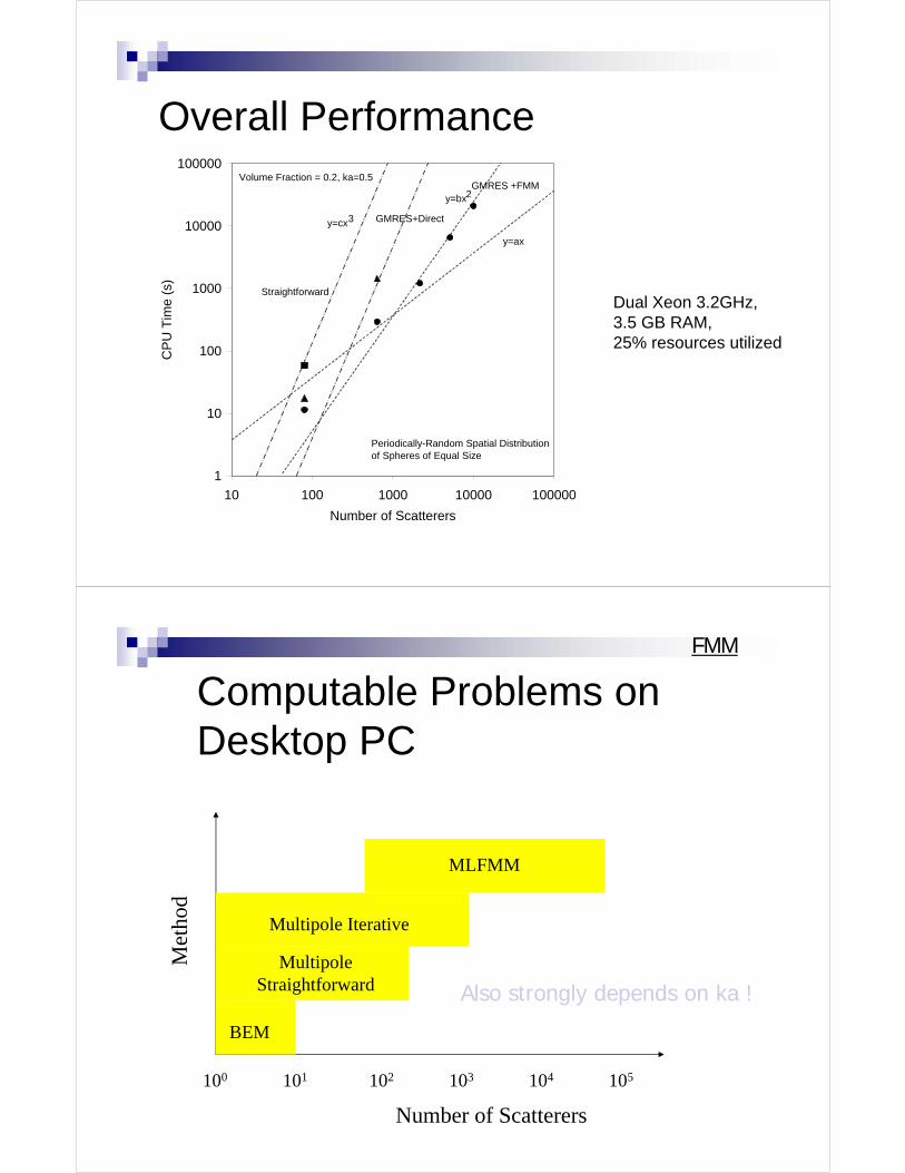
Overall Performance

Dual Xeon 3.2GHz,3.5 GB RAM,25% resources utilized

1

10

100

1000

10000

100000

10 100 1000 10000 100000

Number of Scatterers

CP

U T

ime

(s)

Volume Fraction = 0.2, ka=0.5

Periodically-Random Spatial Distributionof Spheres of Equal Size

GMRES +FMM

Straightforward

y=cx3 GMRES+Direct

y=bx2

y=ax

Computable Problems on Desktop PC

FMM

Met

hod

Number of Scatterers

101 102 103100 104 105

BEM

Multipole Straightforward

Multipole Iterative

MLFMM

Also strongly depends on ka !

Conclusions

We developed, implemented, and tested the Multilevel Fast Multipole Method for computation of multiple scattering problems.Performance of the method depends on a number of controlling parameters. At proper selection of these parameters fast and accurate results can be achieved.Some convergence problems in iterative methods were observed for short wave propagation in regularly spaced sphere grids. This may be due to some internal resonances, which should be investigated.

Future work

Development of faster translation algorithms, covering higher frequencies;Extension for non-spherical scatterrers;Comparisons with continuum (averaging) theories and theories of wave propagation in random media;Computations of acoustic fields in disperse systems (bubbly liquids, particulate systems);Comparisons with experimental data.