Master Sciences de la Matiere

Ecole Normale Superieure de LyonUniversite Claude Bernard Lyon

Stage 2008/2009M2 Physique fondamentale

Computation of meson masses on the lattice

Author:

Roman Welsing

Amselstrasse 8D-46325 Borkenroman.welsing@desy.de

Supervisor:

Dr. Karl Jansen

NIC, DESY, ZeuthenPlatanenallee 6

D-15738 Zeuthen

Abstract

In this report we will present the computation of meson masses on the lattice.

To do so we first discuss the calculation of correlation functions from first principles by means of numer-

ical methods. After a short introduction, we will address the lattice action we have used and how we

can extract a physical mass, for the pion namely, from a correlation function. The correlator is given by

a statistical expectation value over contractions of fermionic propagators, which we calculate.

We further investigate the use of stochastic methods. We discuss how to calculate a reliable error for

the statistical and stochastic mean value and from the resulting error, that we present, we deduce how

to optimize the use of the introduced methods.

KEYWORDS:

Quantum Chromodynamics, Lattice QCD, Wilson fermions, Twisted mass,

HMC algorithm, Pion mass, Stochastic sources, Jackknife error

Zeuthen(Berlin), August 31, 2009

Contents

1 Introduction 21.1 Purpose of the project . . . . . . . . . . . . . . . . . . . . . . . . . . . . . . . . . . . . . . . . 21.2 A look at continuum QCD and its phenomenology . . . . . . . . . . . . . . . . . . . . . . . . 3

2 Lattice QCD 42.1 Numerical Path integrals . . . . . . . . . . . . . . . . . . . . . . . . . . . . . . . . . . . . . . . 42.2 Formulation of the lattice action . . . . . . . . . . . . . . . . . . . . . . . . . . . . . . . . . . 72.3 Spectroscopy of pion masses . . . . . . . . . . . . . . . . . . . . . . . . . . . . . . . . . . . . . 10

3 Simulation and Analysis Details 123.1 Cutoff-effects and improvement . . . . . . . . . . . . . . . . . . . . . . . . . . . . . . . . . . . 123.2 Monte-Carlo errors and jackknife . . . . . . . . . . . . . . . . . . . . . . . . . . . . . . . . . . 123.3 Use of stochastic sources . . . . . . . . . . . . . . . . . . . . . . . . . . . . . . . . . . . . . . . 13

4 Error studies 15

5 Final results 18

6 Conclusions 20

A Monte-Carlo methods 21A.1 Markov chains . . . . . . . . . . . . . . . . . . . . . . . . . . . . . . . . . . . . . . . . . . . . 21A.2 HMC algorithm . . . . . . . . . . . . . . . . . . . . . . . . . . . . . . . . . . . . . . . . . . . . 22

B Gauge fields on the lattice 23B.1 Abelian gauge fields on the lattice . . . . . . . . . . . . . . . . . . . . . . . . . . . . . . . . . 23B.2 Gauge field action and the Wilson loop . . . . . . . . . . . . . . . . . . . . . . . . . . . . . . . 24B.3 Non-Abelian gauge fields on the lattice . . . . . . . . . . . . . . . . . . . . . . . . . . . . . . . 25

C O(a) improvement 26

D Pion operators in twisted basis 27

1

1 Introduction

1.1 Purpose of the project

The subject of this report is to study and understand the computation of meson masses on the lattice. Thiswe have achieved by the calculation of correlation functions from first principles by means of numericalmethods [Section 2.1]. We have namely run a Hybrid-Monte-Carlo algorithm (HMC) [Appendix A] to creategauge field configurations distributed according to a Boltzman factor e−S , given by the action S. Hence thecorrelator is given by a statistical expectation value over contractions of fermionic propagators, which wecalculate analytically [Section 2.3]. They depend on the gauge fields and are obtained by inverting the latticeDirac operator using the conjugate gradient method. We have considered the mass degenerate isospin tripletof pions π0,±. In the twisted-mass formulation of lattice QCD flavour symmetry is broken and therefore thecorrelation functions of the π± and the π0 differ by so called disconnected diagrams, which vanish in thecontinuum limit, where flavour symmetry is restored. The main task therefore consisted in the investigationof stochastic methods [Section 3.3] for the computation of the disconnected diagram contributions to the π0

mass. The goal was to understand and optimize these methods regarding statistical errors in gauge fieldscompared to the stochastic noise and taking into account the computational cost and runtime [Sections 3.2and 4]. Therefore the approach was quite general in view of a further investigation of disconnected diagramsof the η′ meson correlator, because the computation of the η′ mass [7] will be one of the major topics of myongoing work for my diploma thesis. The η′ mass is of particular interest in QCD since its mass originatesto a large extent from topological effects of the gauge fields.From a practical point of view, after getting familiar with the existing code, I have started to compute theπ± correlator in the twisted-mass formulation of lattice QCD [Section 2.2] on a 43 × 8 discrete space-timelattice. In order to do this I have evaluated the fermionic path integral [Section 2.3] obtaining the up anddown quark propagators after Wick contracting the corresponding field operators in the correlation function.I have learned to use and modify existing packages for writing, reading and inverting standard point sourcesand have then implemented the code performing those contractions. When going to the case of the neutralπ0 sector I have found, in order to get reasonable errors, I would need stochastic methods [Section 3.3]to calculate the contributions from disconnected quark diagrams to the correlator function. Hence I havewritten my own code writing and reading stochastic sources and performing the inversions and contractionsusing scripts, namely adapted to a batch farm at DESY Zeuthen. Once I had understood those techniques, Ihave studied the dependence of error estimates on the number of gauge fields and stochastic sources [Section4], quantifying the error by Monte-Carlo and jackknife error methods [Section 3.2]. I have implemented thecorresponding code. After I had understood the uncertainties in the numerical computation it was my goalto show how to obtain a physical value for the pion mass. In general our observables are depending on latticeartefacts, such as finite size and cutoff-effects, so this will be achieved by calculating reliable pion masses atseveral lattice spacings and extrapolating to the continuum limit [Section 3.1 and Section 5].

Acknowledgements

I am happy to say, that I have received a lot of help during the great time I had atDESY Zeuthen.I would therefore like to thank Karl Jansen, not only for his support and for acceptingme as a student, but also for his incredible patience. I thank Dru Renner and CarstenUrbach for guiding me through the sometimes very dark woods of Lattice QCD. I alsoappreciate the help I have received from Simon Dinter, who always kept his good mooddespite all my sometimes stupid questions.Last but not least I would like to thank the teachers of the Ecole Normale Superieurede Lyon for their commitment and for their teaching enthusiasm for research as well.In particular I am grateful to Thierry Dauxois and Aldo Deandrea. Of course I mustthank Edith Thurel a whole lot for she has solved all the not only bureaucratic problemsa student and a foreigner sometimes has to face.Anyway I appreciate the hospitality I have enjoyed in France.

2

1.2 A look at continuum QCD and its phenomenology

Historically one has first studied the structure of hadronic matter by colliding protons with protons. Insuch experiments one has found, that the corresponding cross section is in extremely good agreement witha model of non interacting quarks constituting the nucleon. On the other hand one has found a large rateof hard scattering processes with high transversal momentum (arising from a higher interaction energy)in proton electron collisions, which are especially sensitive to electric charge. Those two phenomena haveresulted in the parton model. It consists in the assumption that nuclei are formed by a small number of pointlike partons, interacting only weakly via the strong interaction but having electric charge. This absence ofstrong interactions in the high energy regime, called asymptotic freedom is one of the most characteristicfeatures of the physics of quarks.The only asymptotically free field theories found to date are non-Abelian gauge theories, proposed by ’tHooft, Politzer, Gross and Wilczek in the 1970s as a candidate for the theory of strong interactions. Thevector boson exchange particles, so called gluons, were found to be the key to the understanding of quarksand their interactions.While Abelian gauge theories in general lead to a screening effect of the charge produced by the vacuumpolarization, only non-Abelian gauge theories can have self interactions of the vector bosons which lead toa growth of the charge with distance called anti-screening. Hence at small distances, or high energies, thecharge gets smaller, which leads to asymptotic freedom, while for low energies a phenomenon called quarkconfinement occurs: the charge grows larger and the strong interactions are gluing the quarks together.Finally, once we accept that non-Abelian gauge theories can describe these phenomena, the question ariseswhich correct gauge symmetry we want to choose. It turns out that the group SU(3) is most promising. Thequarks are found to carry a colour charge, while hadronic matter is colourless, i.e. baryons and mesons arecolour singlets.Accordingly this theory is called QCD, Quantum chromodynamics.The QCD Lagrangian is given by:

LQCD = −1

4[FBµνF

Bµν ] +∑

f

[qf (iγµDµ −mf )qf ] (1)

Where we have omitted the sum over the eight members of the colour octet, denoted by B in the fieldstrength, and f represents the quark flavour index (f= up, down, strange, charm, bottom, top) arising fromthe six Dirac terms for all quark fermions and Dµ = ∂µ − igAµ is the covariant derivative.Quantum chromodynamics has a number of interesting properties, relevant for our understanding of hadronicspectra. Chiral invariance stands out in a most prominent place among them. For example let us consideronly the light (up and down quark) sector. If we assume that the masses of the up and the down quark arezero mu = md = 0, there is a global chiral symmetry leading to a conservation of the axial vector currents:

Afµ = qγµγ5

τf

2q (2)

where we have introduced SU(2) flavour generators τ for f=1,2,3.In reality, however, the axial SU(2)A symmetry is broken. Thus the axial current conservation is violatedby a term proportional to the mass mπ of the pion field (with flavour g):

< 0|∂µAfµ|πg >= −fπm

2πδfg (3)

This is called the PCAC hypothesis (Partially Conserved Axial Current).

Hence we see that the pion mass mπ is a direct measure of the breaking of the axial SU(2)A symme-try, so we can conclude that it is very important to determine the value of the pion mass mπ. Therefore thecomputation of the pion mass mπ from first principles lattice QCD simulations is exactly the topic of thiswork.

3

2 Lattice QCD

Since Kenneth Wilson in 1974 and then Michael Creutz and others have first established the formulationof Quantum Chromodynamics on the lattice, they have paved the way for the study of non-perturbativephenomena by means of numerical methods. Nowadays with increasing computational power, Lattice QCDpromises to answer such questions as whether QCD can explain quark confinement, whether it predicts thecorrect hadron spectrum or also if it accounts for the phase transition to a quark-gluon plasma at sufficientlyhigh temperatures.

2.1 Numerical Path integrals

Lattice QCD is Quantum Chromodynamics, the theory of quarks and gluons and their interactions, formu-lated on a discrete space-time lattice.The starting point is to use Feynman’s path integral approach to quantization. Since the Hamiltonian formal-ism works with non-commuting operators, this approach, which uses only classical fields, is more amenableto direct numerical calculations. Moreover the path integral formalism is symmetric between space and timeand after Wick rotating from real to imaginary time establishes a close connection between Quantum FieldTheory and Statistical Mechanics. This analogy proves itself to be valuable, because it allows for the use ofwell known methods from statistical mechanics.The information of the quantum theory, for example of a scalar field φ, is contained in the Green functions:

G(x, y, z, ...) =< Ω|T (φ(x)φ(y)φ(z)...)|Ω > , (4)

where Ω denotes the ground state. Their path integral representation is (by insertion of complete sets ofstates and use of the path integral representation of the propagator) found to be:

G(x, y, z, ...) =

∫

Dφφ(x)φ(y)φ(z)...eiS[φ]

∫

DφeiS[φ], (5)

where the action S = − 12

∫

d4xφ(x)(2 +M2)φ(x) results from the classical equations of motion(2 +M2)φ(x) = 0 by the action principle δS = 0. More generally also a potential V (φ(x)) can be added,which is, however left out here. If we now, by Wick rotating in the complex plane, continue to imaginarytime x0 → −ix4 the Green functions of Minkowski space become in Euclidean space:

< φ(x)φ(y)φ(z)... >=

∫

Dφφ(x)φ(y)φ(z)...e−SE [φ]

∫

Dφe−SE [φ], (6)

with the Euclidean action given by SE [φ] = 12

∫

d4xφ(x)(−2 +M2)φ(x). The Green functions of Minkowskispace therefore in Euclidean space take the well known form of correlation functions of Statistical Mechanicsdefined by the partition function Z =

∫

Dφe−SE [φ]. One can show that after Wick rotating from real toimaginary time, this imaginary time takes the role of the inverse β = 1

kBT of the temperature T in StatisticalMechanics.By looking at the quantum mechanical propagator Zfi =< φf |e−HT |φi >∼

∫

D[φ]e−S[φ] we identify thepartition function of this system to be:

Z =

∫

dφ < φ|e−HT |φ >= Tre−HT =

∫

D[φ]e−SE [φ] , (7)

where from now on T denotes the time extent. And hence we deduce that also in the general case of ouranalogy we can replace the inverse Temperature β by the time extent T:

β=T . (8)

We have by now noticed from the representation of the correlation functions, that there is a very closeconnection between classical Statistical Mechanics and quantum theory, which is revealed by Feynman’spath integral approach.

4

We can thus employ simulation techniques which have proven to be useful in Statistical Mechanics already.But first let us give a precise mathematical definition of what we have called a path integral, by introducing alattice, i.e. by discretizing the Euclidean space-time with a lattice spacing ”a”. This is done by the followingreplacements:

xµ → nµa (9)

φ(x) → φ(na) (10)∫

d4x→ a4∑

n

(11)

2φ(x) → 1

a2ˆ2φ(na) (12)

Dφ→∏

n

dφ(na) , (13)

where the dimensionless lattice Laplacean ˆ2 is defined as:

ˆ2 =∑

µ

(φ(na+ µa) + φ(na+ µa) − 2φ(na)) . (14)

We can now obtain a path integral expression for the correlator which involves only the dimensionlessquantities φn = aφ(na) and M = aM :

< φnφm... >=

∫∏

l dφlφnφm...e−SE[φ]

∫ ∏

l dφle−SE[φ], (15)

where we have introduced the discretized Euclidean action:

SE = −1

2

∑

n,µ

φnφn+µ +1

2(8 + M2)

∑

n

φnφn =1

2

∑

n,m

φnKnmφm , (16)

with Kmn = −∑4

µ=1[δn+µ,m + δn−µ,m − δn,m] + M2δn,m. These integrals can obviously be evaluatedanalytically. For example by considering the generating functional,

Z0[J ] =

∫

∏

l

dφle−SE[φ]+

P

n Jnφn =1√detK

e12

P

n,m JnK−1nmJm (17)

we obtain the two-point function of scalar field theory as:

< φnφm >= (δ2

δJnδJmZ0[J ])J=0 = K−1

nm . (18)

Now let us briefly discuss the case of Quantum Chromodynamics. As in the case of the scalar field, for freefermionic fields the correlation functions are given by the path integral representation,

< Ψα(n)...¯Ψβ(m)... >=

∫∏

k,γ D ¯Ψγ(k)

∏

l,δ DΨδ(l)Ψα(n)...¯Ψβ(m)...e−SF

∫∏

k,γ D ¯Ψγ(k)

∏

l,δ DΨδ(l)e−SF

, (19)

where the Ψ are the anticommuting fermionic 4-component fields which in the path integral formulationare represented by anticommuting Grassmann numbers and SF is the corresponding Euclidean action. Thecorrelation functions can always be derived from a generating functional,

Z[η, η] =

∫

D ¯Ψ

∫

DΨe−SF +P

n,α[ηα(n)Ψα(n)+¯Ψα(n)ηα(n)] = det[K]e

P

n,m,α,β ηα(n)K−1αβ

(n,m)ηβ(m) , (20)

with Grassmann valued sources ηα(n) and ηα(n).

5

In the general case, where we include interactions, the partition function of Quantum Chromodynamicshas to include a path integral over gauge fields U. The gauge fields U are the quantum fields representing theexchange particles called gluons, carrying the colour charge in interactions of quarks. Therefore we introducea kinetic term for the self interacting gluons, the gauge field action SG[U ].Overall we thus have deduced a partition function:

Z =

∫

DU∫

D ¯Ψ

∫

DΨe−SG[U ]−SF [Ψ,¯Ψ,U ] . (21)

After integrating out the fermionic Grassmann valued part of the path integral [Section 2.3], the pathintegral

∫

DU over gauge fields still remains. We have found that the correlation functions can be derivedfrom a partition function. Hence the calculation of an expectation value of an observable O in lattice QCDcorresponds to the computation of an ensemble average over gauge fields:

< O >=

∫

DUOe−Seff [U ]

∫

DUe−Seff [U ], (22)

with the effective action:Seff [U ] = SG[U ] − ln(detK[U ]) . (23)

Here SG[U ] is again the non-Abelian gauge field action on the lattice, and K is the kernel of the fermionicpart of the action. Note that due to the Grassmann integration rules, in Equation (20) the determinant ofK appears in the numerator, in contrast to the bosonic case, where there is an inverse square root of thedeterminant in the denominator. Of course in order to evaluate this path integral one would have to performa very large number of integrations. For example if we consider 104 space-time lattice points for a SU(3)theory there are roughly 4 x 104 links between these lattice points each with 8 gauge field degrees of freedom,which gives us a number of 320000 integrations to be done. Hence for 10 integration steps we would haveto calculate 10320000 terms, which is even in the quenched approximation det[K] = 1 impossible [2]. Theidea, is thus, as in Statistical Mechanics, to randomly draw gauge field configurations with a probabilitydistribution,

P (Uk)DU =e−S[U ]DU

∫

DUe−S[U ](24)

given by the Boltzmann factor e−S[U ] so that the ensemble average of O will simply be given by the meanvalue of the operator O evaluated for those configurations:

< O >≃ 1

N

N∑

i=1

O(Ui) . (25)

In the literature this is often refered to as Importance Sampling.Methods to obtain gauge field configurations distributed according to the Boltzmann factor are described inappendix A. Our algorithm of choice is the HMC. [Appendix A.2].It is based on a Markov process [Appendix A.1] which produces a sequence of configurations, which areexactly distributed according to the desired Boltzmann factor.One of the most important problems for numerical calculations is the computation of a reliable error for theabove approximation (25). See [13] for example. We also discuss this issue in section 3.2, where we explainhow to estimate the error with the jackknife method and where we also discuss autocorrelation effects whichlead to underestimation of the error due to correlations in the Markov chain [Appendix A.1]. At this stagewe only want to mention that two seperate configurations in the sequence created by the HMC, can becorrelated, which effectively reduces the statistical number of independent data.

During the rest of this report we will no longer explicitly consider the gauge field action. As the gaugefield action SG[U ] is of numerical importance only, and because in practice gauge field configurations arecomputed for one and for all times only, we refer the interested reader to see Appendix B for further details.In the following we will limit ourselves to the formulation of the fermionic action on the lattice only.

6

2.2 Formulation of the lattice action

While we have seen that the formulation of scalar field theory on the lattice is unproblematic, we willnow show that the task to put fermions on a discrete space-time lattice leads to difficulties. We use theseambiguities to illustrate that we have a freedom regarding which lattice action we want to choose, as longas it leads to the correct continuum limit. We will namely present the so called doubling problem. Thisproblem arises when naively discretizing the fermionic part of the action. To illustrate this, let us considerthe free Dirac field, which in Minkowski space obeys the Dirac equation

(iγµ∂µ −M)Ψ(x) = 0 . (26)

This equation of motion follows from an action, which in Euclidean space reads:

SF [Ψ, Ψ] =

∫

d4xΨ(x)(iγµ∂µ +M)Ψ(x) , (27)

where the Ψ are again the anticommuting fermionic 4-component fields which in the path integral formulationare represented by anticommuting Grassmann numbers.In order to obtain dimensionless variables again, we substitute:

M → 1

aM (28)

Ψα(x) → 1

a3/2Ψα(n) (29)

Ψα(x) → 1

a3/2

¯Ψα(n) (30)

∂µΨα(x) → 1

a5/2∂µΨα(n) , (31)

where ∂µ, the antihermitian lattice derivative, is defined by:

∂µΨα(n) =1

2[Ψα(n+ µ) − Ψα(n− µ)] . (32)

Therefore one gets for the naive lattice action,

SF =∑

n,m,α,β

¯Ψα(n)Kαβ(n,m)Ψβ(m) , (33)

where we have introduced,

Kαβ(n,m) =∑

µ

1

2(γµ)αβ [δm,n+µ − δm,n−µ] + Mδmnδαβ . (34)

Hence the correlation function from the generating functional [Equation (20)] is again found to be,

< Ψα(n)¯Ψβ(m) >= K−1

αβ (n,m) , (35)

which by Fourier transformation becomes,

< Ψα(n)¯Ψβ(m) >= lim

a→0

∫ πa

−πa

d4p

(2π)4[−i∑γµpµ +M ]αβ

∑

µ p2µ +M2

eip(x−y) , (36)

where we have introduced pµ = 1a sin(pµa) which in the continuum limit a→ 0 yields lim

a→0pµ = pµ.

7

-4

-3

-2

-1

0

1

2

3

4

-3 -2 -1 0 1 2 3

com

pari

son

to la

ttice

mom

entu

m

continuum momentum x

Comparison of lattice and continuum momentumsin(a*x)/a

x1/a

Figure 1: Plot of pµ = 1asin(pµa) versus x = pµ in the Brillouin zone [−π

a ,πa ]

Correct continuum limit at x = pµ ≈ 0 - Incorrect continuum limit at x = pµ ≈ πa

But this is only true for momenta pµ contained in the center of the Brillouin zone

−1

2

π

a< pµ <

1

2

π

a(37)

as is shown in Figure 1. Here we can neglect the deviations near the maximum of the sine function, becausethere we have pµ ∼ O( 1

a ) and thus in the continuum limit all deviations are suppressed as pµ is diverging inthe denominator of Equation (36). However in the other parts of the Brillouin zone with momenta

pµ < −1

2

π

a,1

2

π

a< pµ (38)

we can see a deviation of the lattice momentum pµ from the continuum momentum pµ for a → 0. Notethat in Figure 1 pµ again yields a finite value at the corner of the Brillouin zone pµ = π

a , namely for a→ 0:pµ = 0, which is a clear difference.Hence there are contributions to the integral Equation (36) above, given by the corners of the Brillouinzone. In 4 dimensions there is 24 = 16 such corners (e.g. [π

a ,0,0,0], [0,πa ,0,0], [π

a ,πa ,0,0], etc.) one doubling

for each additional dimension, where we have included the origin. The zeros of the sine-function at thesecorners destroy the correct continuum limit as pµ is finite for a→ 0. We thus have 15 additional fermion-likelow momentum modes, which are pure lattice artefacts, actually arising from the fact, that the symmetricdiscretization of the derivatives involves twice the lattice spacing, giving rise to an additional solution withequal eigenvalue. This is called the doubling problem.Of course we are free to choose a different action, given that in the continuum limit it leads to the sametheory. We can thus modify our action by an additional term, first introduced by Wilson in 1975, whichvanishes in the naive continuum limit. Wilson’s action for fermions reads,

S(W )F = SF − r

2

∑

n

¯Ψ(n) ˆ2Ψ(n) =

∑

n,m

¯Ψ(n)K

(W )αβ (n,m)Ψβ(m) , (39)

where

K(W )αβ (n,m) = (M + 4r)δnmδαβ − 1

2

∑

µ

[(r − γµ)αβδm,n+µ + (r + γµ)αβδm,n−µ] . (40)

It is important to stress that in general the partial derivative is replaced by the covariant derivative andhence is depending upon the gauge fields.

8

Moreover we want to formulate a gauge invariant action. Due to the limited room in this report wediscuss this issue in Appendix B and limit ourselves to discuss the free case in this section only.Wilson’s action, in the free case, leads again to the two-point function (36), with M replaced by,M → M(p) = M + 2r

a

∑

µ sin2(pµa/2), and where we still define pµ = 1a sin(pµa).

Now we can see that in the limit a→ 0: M(p) → M except at the corners of the Brillouin zone where M(p)diverges. This eliminates the doubling problem, as the low momentum excited states are suppressed: ∼ 1

M(p)

One disadvantage of this method is that it breaks the chiral symmetry of the action for M=0. A fur-ther problem is that the kernel K can have eigenvalue zero. Therefore the fermionic determinant is equal orin numerical calculations close to zero, det[K] = 0, which means that the according configuration for thispropagator should have a statistical weight zero. But the propagator, the inverse of the Dirac operator,diverges. Such configurations which compromise the validity of our ensemble are called exceptional configu-rations. Hence there are various alternative attempts to formulate actions on the lattice.In these attempts there is a choice to be made. We can sacrifice full chiral symmetry with the advantage oflower computational cost, or we can choose a rather complicated lattice action which keeps chiral symmetry,but which is of course harder to simulate.

One action which uses rather simple Wilson type fermions is the twisted-mass action. One virtue isthat in twisted-mass QCD the exceptional configurations have been removed. Originally twisted-massQCD is a scheme for a doublet of two flavours Nf = 2 where the Wilson type lattice Dirac operator DW isreplaced by:

Dtwist = DW +mq + iµqγ5τ3 . (41)

The isospin operator τ3 acts in flavor space and the parameter µq is called the twisted mass.Now doublers are avoided, as we use Wilson type fermions and moreover exceptional configurations areremoved for µq > 0:

det[Dtwist] = det[(DW +mq)+(DW +mq) + µ2

q] > 0 (42)

One can verify that the continuum twisted mass action,

SF [Ψ, Ψ] =

∫

d4xΨ(x)(γµDµ +mq + iµqγ5τ3)Ψ(x) (43)

under a chiral rotation,χ = eiγ5τ3ω/2Ψ (44)

χ = Ψeiγ5τ3ω/2 (45)

for tan(ω) =µq

mqbecomes,

SF [χ, χ] =

∫

d4xχ(x)(γµDµ +M)χ(x) , (46)

where M =√

m2q + µ2

q.

While for non-zero lattice spacing the twisted-mass term breaks both flavour and parity symmetries, in thecontinuum limit these symmetries are restored. The breaking of the flavor symmetry leads to a mass splittingbetween charged and neutral pions. [Section 2.3] This is explicitly arising from additional contribution ofdisconnected loops to the correlator. These vanish in the continuum limit, where symmetries are restoredwith O(a2) [Section 3.1] at maximal twist: ω = π

2 .Thus one main advantage of Wilson twisted-mass lattice QCD is that at maximal twist we have automaticO(a) improvement. In contrast standard Wilson fermions approach the continuum only at a rate of O(a).Maximal twist can be obtained by tuning:

mq → mq = 0 ⇒ ω =π

2. (47)

This, in practice, is achieved by setting the PCAC mass to zero.

mPCAC =

∑

x < ∂0Aa0(x)P

a(0) >

2∑

x < P a(x)P a(0) >(48)

9

2.3 Spectroscopy of pion masses

The ultimate goal of calculating correlation functions in lattice QCD is to extract values of physical observ-ables such as masses from them. The most general two point correlation function of two observables Oi andOj can in Statistical Mechanics be written,

Cij(t) = Tr[Oi(t)Oj(0)e−βH ]/Z , (49)

with the partition function given by Z = Tr[e−βH ]. Now as we have found β=T , where T is the time extentand β the inverse of the temperature, we can write our two point correlation function as:

Cij(t) =

∑

n e−EnT < n|Oi(t)Oj(0)|n >

∑

n e−EnT

, (50)

which in the ”zero temperature limit” T → ∞ gives just the vaccuum expectation value:

limT→∞

Cij(t) =< 0|Oi(t)Oj(0)|0 > . (51)

After inserting a complete set of states we get by considering the time evolution Oi(t) = eHtOie−Ht:

Cij(t) =∑

n

< 0|Oi|n >< n|Oj |0 > e−(En−E0)t/Z . (52)

Obviously in the large time limit for t→ ∞ the lowest energy states are dominating, which for i=j yields,

Cii ≃ | < 0|Oi|0 > |2 + | < 0|Oi|1 > |2e−(E1−E0)t , (53)

Usually correlation functions are defined with the first vaccuum disconnected part removed:

Cii ≃ | < 0|Oi|1 > |2e−(E1−E0)t , (54)

Therefore the correlation length, which determines the exponential decay rate, is given by the inverse of themass gap:

ζ = (E1 − E0)−1 =

1

am, (55)

Now let us consider the field operator creating charged pions, which are pseudoscalar mesons:

π± = dγ5u . (56)

Since we want to calculate the mass of the charged pion, this leads us directly to the two-point correlationfunction, which can be evaluated from the general case of the generating functional:

< π+(x)π(y) >=< u(x)γ5d(x)d(y)γ5u(y) > (57)

=

∫

DUDuDuDdDd[uγ5ddγ5u]eR

(−uG−1u u−dG−1

dd)+SG/Z (58)

=

∫

DU det[Gu] det[Gd]Gu(x, y)γ5Gd(y, x)γ5e−SG/Z (59)

⇔< π+(x)π(y) >=< u(x)γ5d(x)d(y)γ5u(y) > . (60)

Here we have introduced the Wick contractions equivalent to the path integral.

With u(x)u(y) = Gu(y, x) this leads to the propagator:

< π+(x)π(y) >=< Tr[Gu(x, y)γ5Gd(y, x)γ5] > . (61)

10

Finally the field operator for the neutral pion, which is in a flavour singlet pseudoscalar state, in thetwisted basis [Appendix D] reads:

π0 =1√2(uu+ dd) . (62)

Accordingly the two-point correlation function becomes:

< π+(x)π(y) >=<1

2(u(x)u(x) + d(x)d(y))(u(y)u(y) + d(y)d(y)) > (63)

=1

2[< u(x)u(x)u(y)u(y) > + < d(x)d(x)d(y)d(y) > (64)

+ < d(x)d(x)u(y)u(y) > + < u(x)u(x)d(y)d(y) >] (65)

=1

2[< u(x)u(x)u(y)u(y) > + < d(x)d(x)d(y)d(y) > (66)

+ < u(x)u(x)u(y)u(y) > + < d(x)d(x)d(y)d(y) > (67)

+ < d(x)d(x)u(y)u(y) > + < u(x)u(x)d(y)d(y) >] . (68)

Figure 2: Connected and disconnected quark diagrams

Hence we still have the usual connected contributions now averaged over up and down quarks. But fornon zero lattice spacing, i.e. with broken flavor symmetry, we have disconnected contributions as well.

< π+(x)π(y) >=1

2< Tr[Gu(x, x)]Tr[Gu(y, y)] + Tr[Gu(x, y)Gu(y, x)] + Tr[Gd(x, x)]Tr[Gd(y, y)] (69)

+Tr[Gd(x, y)Gd(y, x)] + Tr[Gu(x, x)]Tr[Gd(y, y)] + Tr[Gd(x, x)]Tr[Gu(y, y)] > (70)

With the identity,Gd(x, y) = γ5G

+u (y, x)γ5 (71)

the disconnected contribution thus becomes,

D =1

2< Tr[Gu +G+

u ]Tr[Gu +G+u ] >= 2 < (Tr[Re(Gu)])2 > , (72)

while for the connected contribution we had,

C =< Tr[Gu(x, y)γ5Gd(y, x)γ5] > . (73)

Keep in mind that in the end we will always consider the correlation function in momentum space at zeromomentum, where we have summed over all space-volume dependences:

C(~p, t) =

∫

d3xei~p~xC(~x, t, 0, 0) (74)

C(t) = C(0, t) ≃∑

~x

C(~x, t, 0, 0) . (75)

11

3 Simulation and Analysis Details

If we want to compare the experimental data for a physical observable to numerical results, one will alwaysfind lattice artefacts. One reason is the finite volume of the lattice. These are finite size effects. Anotherreason is the non zero lattice spacing leading to discretization errors, called cutoff-effects.

3.1 Cutoff-effects and improvement

In practice therefore in order to eliminate the cutoff-effects one will always calculate the physical entityfor several lattice spacing, and extrapolate in dependence of the lattice spacing. We say that we take thecontinuum limit.Hence because of our limited ability to approach the continuum it is often necessary to improve the dis-cretization errors to O(a2) to obtain a sufficient data set. One possiblity to achieve this is the Symanzikimprovement program, another elegant way is to take advantage of automatic O(a) improvement of twisted-mass QCD at maximal twist. We shortly mention these techniques in Appendix C.

3.2 Monte-Carlo errors and jackknife

Another field of great practical significance is the comprehension of statistical standard errors. It is notpossible to overstress the importance of the computation of reliable errors, in order to compare numericalresults to experiment. To do this one first has to gain a comprehension of the goodness of our statisticalMonte-Carlo ensemble, the gauge field configurations. One of the keys to make quantitative estimates of thestatistical independence of our data set is the autocorrelation [9]. If we call our observable quantities aα

and accordingly their exact statistical mean values Aα the autocorrelation function is defined by:

Γαβ(i− j) =< (aiα −Aα)(aj

β −Aβ) > , (76)

where aiα and aj

α are at positions i and j in our sequence of Monte-Carlo generated samples [Appendix A]. Inthe case of the generation of configurations via the Hybrid-Monte-Carlo algorithm HMC this is often referedto as Monte-Carlo time τ . Now we take the mean value aα = 1

N

∑Ni=1 a

iα as the natural estimator for the

primary observables Aα and hence we get for the covariance matrix,

< (aα −Aα)(aβ −Aβ) >=1

N2

N∑

i,j=1

Γαβ(i− j) ≃ 1

N

∑

t

Γαβ(t) ≃ 1

NCαβ + O(

1

N2) , (77)

where we have introduced:

Cαβ =

∞∑

t=−∞Γαβ(t) . (78)

This means that the error σα for the estimate of Aα is to leading order given by the estimate σ2α ≃ 1

NCαα.By introducing the integrated autocorrelation time,

τ intα =

1

2vα

∞∑

t=−∞Γαα(t) (79)

this estimate takes the form,

σ2α =

2τ intα

Nvα , (80)

where vα = Γαα(0) is the naive variance, not taking into account autocorrelation effects. It is corrected forby a factor given by the integrated autocorrelation time and divided by the number of samples to give anaccurate error estimate. Hence it will be our goal to minimize the integrated autocorrelation time, by takinginto account only those configurations which are uncorrelated, i.e. where the autocorrelation time is equalto unity: 2τ int = 1. In the simulation this is realized by skipping a certain number of trajectories, or config-uration samples, before saving the next one, which should not be correlated to the previous one beeing saved.

12

Thus now in principle we are in the position to calculate the errors of the ensemble average over config-urations. For the correlation function, where we have to calculate several ensemble averages, this wouldmean, that for each configuration we compute a correlator, after that the naive variance, which we devideby the number of samples. But actually, when we have derived the form the correlation function takes in thecontinnuum, we had to substract the vaccuum expectation value of the disconnected part. For the neutral

pion this contribution takes the form < 0|π(0)|0 >2= < 1

2 (Tr[Gu(0, 0)] + Tr[Gd(0, 0)]) >2. We will see that

it is of the order of magnitude of the disconneted correlator. Hence we substract two correlated big numbers,to give a third small number. If we calculate the error of the difference by means of simple error propagationit will be unsignificantly big, as we would simply have to add the absolute errors.

In contrast to that we can compute the real statistical error by a method called the jackknife [11], whichtakes into account the statistical correlations of the terms we substract. Suppose for example that wewant to compute the error for an estimator θ = s(C) where we have a sample C of N configurationsC = (C1, C2, C3, ..., CN ). Then we define the jackknife samples:

C(i) = (C1, C2, C3, ..., Ci−1, Ci+1, ..., CN ) , (81)

where the i-th jackknife sample constists of the whole data set with configuration Ci removed. Accordinglywe call θi = s(C(i)) the jackknife replicas of θ. After introducing the mean

θ(∗) =

N∑

i=1

θ(i)/N (82)

of jackknife replicas we finally find that the jackknife estimate of the standard error takes the form:

σjack =

√

√

√

√

N − 1

N

N∑

i=1

(θ(i) − θ(∗))2 . (83)

By considering the special case θ = x for the estimator, we observe that here the error of the mean value is:

σjack =

√

√

√

√

1

N(N − 1)

N∑

i=1

(x(i) − x)2 , (84)

because θ(∗) = x and θ(i) = NN−1 x− x(i)

N−1 .

This motivates the prefactor of (N −1)/N . We could of course also use the prefactor [(N −1)/N ]2 to obtainthe usual standard error estimate for the mean given by:

σx =

√

√

√

√

1

N2

N∑

i=1

(x(i) − x)2 . (85)

But the jackknife convention will for large N clearly coincide whith this choice yealding the standard error.

3.3 Use of stochastic sources

In the final part of this section we would like to discuss a last tool of great importance for the computationof the fermionic propagators. The naive way to calculate a fermion propagator is as follows. We have seenthat the propagator extracted from the path integration of the fermionic Grassmann variables is nothingbut the inverse of the Dirac operator:

6D(x, y)−1 = G(x, y) . (86)

13

So let us consider a spinor Ψj(x) with space-time indices x and and spin and colour indices j, which afterthe action of the Dirac operator on it yields a δ-function:

6D(x, y)jkΨj(x) = δk(y) (87)

δ-function here means that we have a matrix with one entry at position (x,k) only, which in the followingwe refer to as a point-source. By solving Equation (89) for Ψj(x) we can obtain one column vector Ψj(x) ofthe propagator matrix G called one-to-all propagator:

Ψj(x) = Gjk(x, y)δk(y) (88)

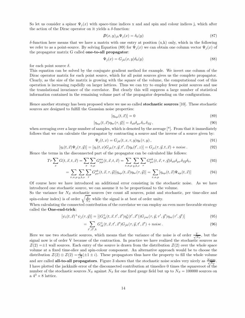
for each point source δ.This equation can be solved by the conjugate gradient method for example. We invert one column of theDirac operator matrix for each point source, which for all point sources gives us the complete propagator.Clearly, as the size of the matrix is growing with the square of the volume, the computational cost of thisoperation is increasing rapdidly on larger lattices. Thus we can try to employ fewer point sources and usethe translational invariance of the correlator. But clearly this will suppress a large number of statisticalinformation contained in the remaining volume part of the propagator depending on the configurations.

Hence another strategy has been proposed where we use so called stochastic sources [10]. These stochasticsources are designed to fulfill the Gaussian noise properties:

[ηaµ(t, ~x)] = 0 (89)

[ηaµ(t, ~x)ηbν(τ, ~y)] = δabδµνδtτ δ~x~y , (90)

when averaging over a large number of samples, which is denoted by the average [*]. From that it immediatelyfollows that we can calculate the propagator by contracting a source and the inverse of a source given by:

Ψj(t, x) = Gjk(t, x, τ, y)ηk(τ, y) , (91)

[ηi(t, ~x)Ψj(τ, ~y)] = [ηi(t, x)Gjk(τ, ~y, t′, ~z)ηk(t′, z)] = Gji(τ, ~y, t, ~x) + noise . (92)

Hence the terms in the disconnected part of the propagator can be calculated like follows:

Tr∑

x

G(t, ~x, t, ~x) =∑

x

∑

a,µ

Gaaµµ(t, ~x, t, ~x) =

∑

x,a,µ

∑

y,b,ν

∑

τ

Gabµν(t, ~x, τ, ~y)δabδµνδ~x~yδtτ (93)

=∑

x,a,µ

∑

y,b,ν

∑

τ

Gabµν(t, ~x, τ, ~y)[ηaµ(t, ~x)ηbν(τ, ~y)] =

∑

x,a,µ

[ηaµ(t, ~x)Ψaµ(t, ~x)] (94)

Of course here we have introduced an additional error consisting in the stochastic noise. As we haveintroduced one stochastic source, we can assume it to be proportional to the volume.So the variance for NS stochastic sources (we count all sources, point and stochastic, per time-slice and

spin-colour index) is of order√

VNS

while the signal is at best of order unity.

When calculating the connected contribution of the correlator we can employ an even more favorable strategycalled the One-end-trick:

[ψi(t, ~x)+ψj(τ, ~y)] = [(G+

ik(t, ~x, t′, ~x′)η∗k(t′, ~x′))Gjm(τ, ~y, τ ′, ~y′)ηm(τ ′, ~y′)] (95)

=∑

t′,~x′,k

G+ik(t, ~x, t′, ~x′)Gjk(τ, ~y, t′, ~x′) + noise . (96)

Here we use two stochastic sources, which means that the variance of the noise is of order V√NS

, but the

signal now is of order V because of the contraction. In practice we have realized the stochastic sources asZ(2) =±1 wall sources. Each entry of the source is drawn from the distribution Z(2) over the whole spacevolume at a fixed time-slice and spin-colour component. An alternative approach would be to choose thedistribution Z(2) ⊗ Z(2) = 1√

2(±1 ± i). These propagators thus have the property to fill the whole volume

and are called all-to-all propagators. Figure 3 shows that the stochastic noise scales very nicely as Noise√NS

.

I have plotted the jackknife error of the disconnected contribution at timeslice 0 times the squareroot of thenumber of the stochastic sources NS against NS for one fixed gauge field but up to NS = 100000 sources ona 43 × 8 lattice.

14

0.0001

0.00012

0.00014

0.00016

0.00018

0.0002

0.00022

0.00024

0 10000 20000 30000 40000 50000 60000 70000 80000 90000 100000

Sca

led

Err

or S

qrt(

N)*

Err

or[D

(0)]

Number of stochastic sources N

Errorscaling Plot

"disc.new" using 1:(sqrt($1)*$3)

Figure 3: Errorscaling of the disconnected part of the π0 correlator for one fixed gauge field in dependenceof the number of stochastic sources

4 Error studies

In this section we discuss how to optimize the calculation of meson masses and correlation functions in termsof the error we obtain for a given computational cost.One of the main aspects of my ongoing work was to investigate the error of the connected and disconnectedcontributions to the pion correlator, namely the scaling of this error with the number of stochastic sourcesand the number of gauge fields. I have therefore run the HMC-algorithm, created a certain number of up to1000 configurations and inverted the Dirac operator for these configurations to obtain propagators of pointand stochastic sources.First of all I have found, that the error in the connected contributions to the pion correlator compared to thedisconnected contributions is so small, that it is possible to calculate the π± or connected correlator usingpoint sources at a fixed timeslice and volume point only instead of stochastic sources.It is important to note that it is not advantageous to invert point sources at all space time points as is shownin the table below. We have tried to do so and compared the two correlators we have obtained for 10 gaugefields:

Timeslice π± Correlator atfixed volume point

Error in 10 gaugefields

π± Correlator forall point sources

Error in 10 gaugefields

0 1.28337 0.00319 1.28230 0.0007141 0.144515 0.001041 0.143443 0.00035422 0.0135875 0.0003457 0.0138218 0.00006693 0.00140426 0.00005038 0.00146531 0.000011214 0.000306584 0.00001084 0.000312552 0.00000426

Hence by increasing the inversions by a factor L × L × L × T we improve the error by a factor of 4 only.This could also have been achieved by taking 16 times the number of gauge fields and hence increasing thenumber of inversions by a factor of only 16, where we assume that the error scales as expected in the numberof gauge fields. This we will see later.

15

In practice this strategy is necessary too, because considering the available disk space it is not possibleto store or create point one-to-all propagators for hundreds of gauge fields times with a space-time volumeof the order of 243 × 48 (which is a typical lattice size).

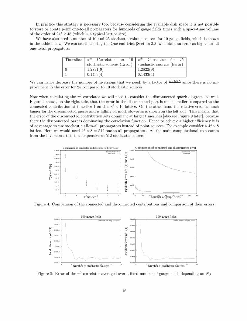
We have also used a number of 10 and 25 stochastic volume sources for 10 gauge fields, which is shownin the table below. We can see that using the One-end-trick [Section 3.3] we obtain an error as big as for allone-to-all propagators:

Timeslice π± Correlator for 10stochastic sources (Error)

π± Correlator for 25stochastic sources (Error)

0 1.2831(9) 1.2822(9)1 0.1433(4) 0.1433(4)

We can hence decrease the number of inversions that we need, by a factor of L×L×L10 since there is no im-

provement in the error for 25 compared to 10 stochastic sources.

Now when calculating the π0 correlator we will need to consider the disconnected quark diagrams as well.Figure 4 shows, on the right side, that the error in the disconnected part is much smaller, compared to theconnected contribution at timeslice 1 on this 83 × 16 lattice. On the other hand the relative error is muchbigger for the disconnected pieces and is falling off much slower as is shown on the left side. This means, thatthe error of the disconnected contribution gets dominant at larger timeslices [also see Figure 9 later], becausethere the disconnected part is dominating the correlation function. Hence to achieve a higher efficiency it isof advantage to use stochastic all-to-all propagators instead of point sources. For example consider a 43 × 8lattice. Here we would need 43 × 8 = 512 one-to-all propagators . As the main computational cost comesfrom the inversions, this is as expensive as 512 stochastic sources.

0

5e-06

1e-05

1.5e-05

2e-05

2.5e-05

3e-05

3.5e-05

4e-05

4.5e-05

5e-05

5.5e-05

3 4 5 6 7 8

C(t

) an

d D

(t)

Timeslice t

Comparison of connected and disconnected correlatordisconnected

connected

0

2e-05

4e-05

6e-05

8e-05

0.0001

0 100 200 300 400 500 600 700 800

Jack

knif

e er

ror

of C

(1)

and

D(1

)

Number of gauge fields

Comparison of connected and disconnected errordisconnected

connected

Figure 4: Comparison of the connected and disconnected contributions and comparison of their errors

0.000137

0.000138

0.000139

0.00014

0.000141

0.000142

0.000143

0.000144

0.000145

0 5 10 15 20 25 30

Jack

knif

e er

ror

of C

(1)

Number of stochastic sources

100 gauge fields"outcon100.dat" using 1:4

7.1e-05

7.2e-05

7.3e-05

7.4e-05

7.5e-05

7.6e-05

7.7e-05

7.8e-05

0 5 10 15 20 25 30

Jack

knif

e er

ror

of C

(1)

Number of stochastic sources

300 gauge fields"outcon300.dat" using 1:4

Figure 5: Error of the π0 correlator averaged over a fixed number of gauge fields depending on NS

16

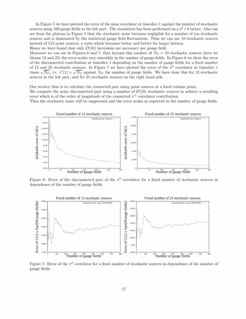
In Figure 5 we have plotted the error of the pion correlator at timeslice 1 against the number of stochasticsources using 100 gauge fields in the left part. The simulation has been performed on a 43×8 lattice. One cansee from the plateau in Figure 5 that the stochastic noise becomes negligible for a number of ten stochasticsources and is dominated by the statistical gauge field fluctuations. Thus we can use 10 stochastic sourcesinstead of 512 point sources, a ratio which becomes better and better for larger lattices.Hence we have found that only O(10) inversions are necessary per gauge field.Moreover we can see in Figures 6 and 7, that beyond this number of NS = 10 stochastic sources (here wechoose 12 and 25) the error scales very smoothly in the number of gauge fields. In Figure 6 we show the errorof the disconnected contribution at timeslice 1 depending on the number of gauge fields for a fixed numberof 12 and 25 stochastic sources. In Figure 7 we have plotted the error of the π0 correlator at timeslice 1times

√NG, i.e. C(1) ×

√NG against NG the number of gauge fields. We have done this for 12 stochastic

sources in the left part, and for 25 stochastic sources on the right hand side.

Our stratey thus is to calculate the connected part using point sources at a fixed volume point.We compute the noisy disconnected part using a number of O(10) stochastic sources to achieve a resultingerror which is of the order of magnitude of the connected π± correlator contribution.Then the stochastic noise will be suppressed and the error scales as expected in the number of gauge fields.

2e-06

4e-06

6e-06

8e-06

1e-05

1.2e-05

1.4e-05

1.6e-05

1.8e-05

2e-05

0 50 100 150 200 250 300

Jack

knif

e er

ror

of D

(1)

Number of gauge fields

Fixed number of 12 stochastic sources"outputstos12.dat" using 2:6

0

5e-06

1e-05

1.5e-05

2e-05

2.5e-05

3e-05

0 50 100 150 200 250 300

Jack

knif

e er

ror

of D

(1)

Number of gauge fields

Fixed number of 25 stochastic sources"outputstos25.dat" using 2:6

Figure 6: Error of the disconnected part of the π0 correlator for a fixed number of stochastic sources independence of the number of gauge fields

0.001

0.0011

0.0012

0.0013

0.0014

0.0015

0.0016

0 100 200 300 400 500 600 700 800

Err

or o

f C

(1)

x Sq

rt[#

Gau

ge-f

ield

s]

Number of gauge fields

Fixed number of 12 stochastic sources"outputstos12.dat" using 2:($4*sqrt($2))

0.0009

0.001

0.0011

0.0012

0.0013

0.0014

0.0015

0.0016

0 100 200 300 400 500 600 700 800

Err

or o

f C

(1)

x Sq

rt[#

Gau

ge-f

ield

s]

Number of gauge fields

Fixed number of 25 stochastic sources"outputstos25.dat" using 2:($4*sqrt($2))

Figure 7: Error of the π0 correlator for a fixed number of stochastic sources in dependence of the number ofgauge fields

17

1.4

1.6

1.8

2

2.2

2.4

2.6

2.8

3

3.2

0 5 10 15 20

a x

m

Number of stochastic sources

Fit of pion mass"massfit.dat"

-0.0005

0

0.0005

0.001

0.0015

0.002

0.0025

0.003

0.0035

0.004

0 2 4 6 8 10 12 14 16

C(t

)

t

Fit of the correlator"overall.dat"

f(x)

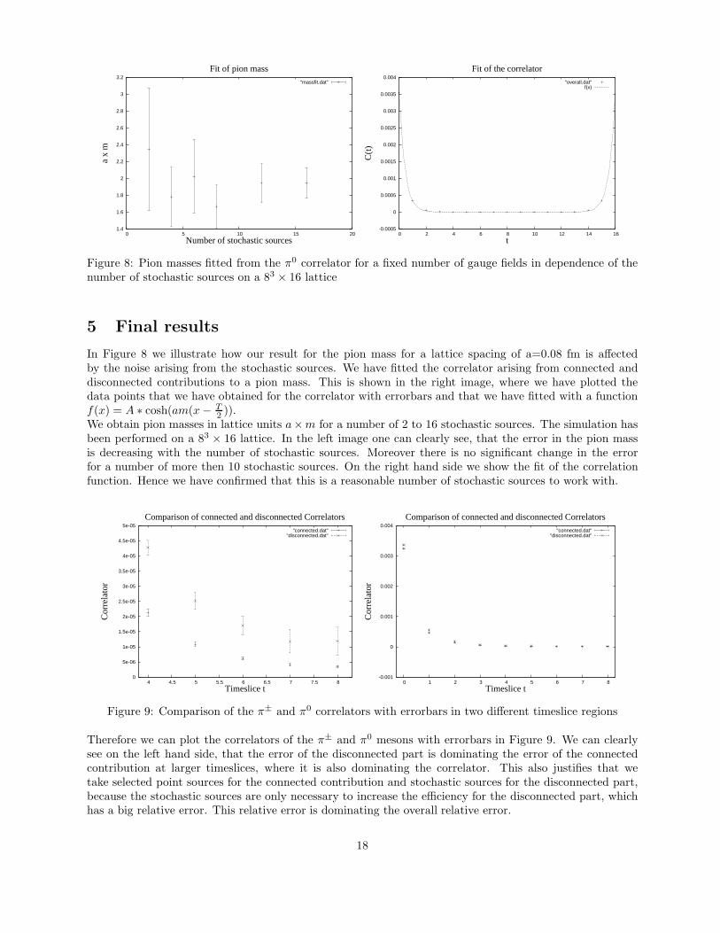
Figure 8: Pion masses fitted from the π0 correlator for a fixed number of gauge fields in dependence of thenumber of stochastic sources on a 83 × 16 lattice

5 Final results

In Figure 8 we illustrate how our result for the pion mass for a lattice spacing of a=0.08 fm is affectedby the noise arising from the stochastic sources. We have fitted the correlator arising from connected anddisconnected contributions to a pion mass. This is shown in the right image, where we have plotted thedata points that we have obtained for the correlator with errorbars and that we have fitted with a functionf(x) = A ∗ cosh(am(x− T

2 )).We obtain pion masses in lattice units a×m for a number of 2 to 16 stochastic sources. The simulation hasbeen performed on a 83 × 16 lattice. In the left image one can clearly see, that the error in the pion massis decreasing with the number of stochastic sources. Moreover there is no significant change in the errorfor a number of more then 10 stochastic sources. On the right hand side we show the fit of the correlationfunction. Hence we have confirmed that this is a reasonable number of stochastic sources to work with.

0

5e-06

1e-05

1.5e-05

2e-05

2.5e-05

3e-05

3.5e-05

4e-05

4.5e-05

5e-05

4 4.5 5 5.5 6 6.5 7 7.5 8

Cor

rela

tor

Timeslice t

Comparison of connected and disconnected Correlators"connected.dat"

"disconnected.dat"

-0.001

0

0.001

0.002

0.003

0.004

0 1 2 3 4 5 6 7 8

Cor

rela

tor

Timeslice t

Comparison of connected and disconnected Correlators"connected.dat"

"disconnected.dat"

Figure 9: Comparison of the π± and π0 correlators with errorbars in two different timeslice regions

Therefore we can plot the correlators of the π± and π0 mesons with errorbars in Figure 9. We can clearlysee on the left hand side, that the error of the disconnected part is dominating the error of the connectedcontribution at larger timeslices, where it is also dominating the correlator. This also justifies that wetake selected point sources for the connected contribution and stochastic sources for the disconnected part,because the stochastic sources are only necessary to increase the efficiency for the disconnected part, whichhas a big relative error. This relative error is dominating the overall relative error.

18

1

10

100

1000

10000

100000

0 0.2 0.4 0.6 0.8 1 1.2

C(t

)

Physical time t[fm]

Connected Correlator12x12x12x24

8x8x8x166x6x6x12

1

10

100

1000

10000

100000

0 0.2 0.4 0.6 0.8 1 1.2

C(t

)

Physical time t[fm]

Disconnected Correlator12x12x12x24

8x8x8x166x6x6x12

Figure 10: Plot of the scaled π± and π0 correlators with errorbars

Finally we have computed the disconnected and connected correlators at lattice spacings of a=0.1 fmon a 63 × 12 lattice, at a=0.08 fm on a 83 × 16 lattice and at a=0.065 fm on a 123 × 24 lattice. We havescaled these correlators of dimension 6 according to the lattice spacing and plotted them against physicaltime tphys = t× a in Figure 10. Unfortunately there is a slight mismatch in the volume of the lattice. Thismismatch is the biggest for the large 123× 24 lattice, so that the corresponding correlator is clearly differingfrom the other two, as you can see in the left part of Figure 10, where we have plotted the π± correlators.In principle, at equal volume, these correlators should coincide, as our parameters are tuned to keep the π±

mass constant for each lattice spacing and we are working at maximal twist such that the lattice spacingartefacts should be very small.

We compare the averaged sum of the scaled correlators in the following table.

Lattice Physical L [fm] a [fm] π± Correlator 1T

∑

t C(t) π0 Correlator 1T

∑

t[C(t)+D(t)]63 × 12 0.61 0.1 886(5) 969(12)83 × 16 0.66 0.082 899(9) 1009(15)123 × 24 0.79 0.065 672(4) 745(10)

Again it can be seen that for the almost matched lattices (63 × 12 at a=0.1 fm and 83 × 16 at a = 0.08 fm)a nice scaling in the lattice spacing is observed while for the unmatched lattice (123 × 24 at a=0.0065 fm)a clear discrepancy is observed. Moreover, there is also a significant difference between the π± and the π0

correlators indicating the inherent parity violation of twisted-mass fermions at non-zero lattice spacings. Inthis report, we could not demonstrate, that this lattice artefact vanishes in the continuum limit and thisquestion will be the subject of my further work.

We have also plotted the π0 correlator in the right part of Figure 10. Here you can see the same ef-fect. We also identify big errorbars in the middle of the plot, arising from the disconnected contributions.As we could use only 3 stochastic sources for the big lattice we can see that on a big lattice this is alreadysufficient, while with 10 stochastic sources on the small lattice we still obtain unsignificant values for thedisconnected contribution at large timeslices. Hence we again can state, that this part of the correlator isnoisy.In principle, at equal volume, one should also be able to show O(a) improvement for these lattice spacings,which means that the π0 mass is depending linear on a2 at small lattice spacings.

19

The pion mass is in general extracted by first of all plotting the effective mass,

meff (t+1

2) = − ln

C(t+ 1)

C(t), (97)

against time. As we have seen in Section 2.3 only in the limit t→ ∞ excited states will be removed. Howeverin the middle of the lattice at t = T

2 we will clearly see finite size effects just arising from our boundary con-

ditions, which lead to the overlap of exponentials e−mat and e−ma(T−t) yielding a cosh(ma(t− T2 )) function.

But, we here are only fitting to an exponential. Hence we are looking for a plateau, where the effects arisingfrom finite size and the excited states are still negligible. We have obtained such a plateau on a 123 × 24lattice. It is shown in Figure 11, where we plot the effective mass meff (t+ 1

2 ) depending on the timeslice t.

-1.5

-1

-0.5

0

0.5

1

1.5

2

2.5

3

3.5

0 2 4 6 8 10 12

Eff

ectiv

e m

ass

t

Effective mass on the 12x12x12x24 lattice"pipluseffmass.dat""pizeroeffmass.dat"

Figure 11: Plot of meff for the π± and π0 correlators with errorbars

One can clearly see that the errorbars of the overall π0 correlator are dominated by the disconnected con-tributions, as they are much bigger than the errorbars of the connected π± part. We also identify the π±

mass to be bigger than the π0 mass, in consistency with results of ref. [5].

6 Conclusions

This project first of all has enlightened my understanding of lattice QCD as a whole, regarding theoreticalfoundations and practical methods.During the period at DESY Zeuthen, I have thus learned how to use methods for the reduction of errors in thecalculation of correlation functions. I have also gained a comprehension on how to extract physical massesfrom these correlation functions. Now I am able to employ stochastic methods to investigate disconnectedquark diagrams, which are important for the computation of the η′ mass in particular. Also I am nowfamiliar with existing code and packages, in view of a further investigation of the η′ mass. I have seen thattwisted-mass QCD breaks flavour symmetry leading to a difference in the π± and π0 mass. It remains toshow that this difference is vanishing with O(a2), as flavour symmetry is restored in the continuum limit,and because of automatic O(a) improvement in maximally twisted-mass QCD. This will be the task for thefollowing weeks to come. At the same time it will be possible to extract the physical mass of the three pionsby taking the continuum limit.However I can conclude that the computation of meson masses from first principles is by now well understoodfor the case of the pion triplet, comprising, in particular, the calculation of the connected and disconnectedcontributions. Thus I am able to proceed now to the calculation of other mesons as well, with a particularfocus of the η′ mass.

20

A Monte-Carlo methods

In this Appendix we briefly discuss methods for the evaluation of path integrals over gauge field configu-rations. If we want to calculate the expectation value of an observable numerically, one standard way isthe Monte-Carlo method. The idea behind is to draw gauge field configurations, denoted by φ, distributedaccording to our Boltzmann factor e−S[φ] with a probability distribution,

P (φk)Dφ =e−S[φ]Dφ

∫

Dφe−S[φ]. (98)

In the literature this is refered to as Importance Sampling. Once we can generate sequences of configu-rations (φk)kǫN fulfilling this probability distribution, the expectation value of our observable O, turns outto be as simple as a sum,

〈O〉 =1

N

N∑

k=1

O(φk) . (99)

In the limit N → ∞ this gives the value of O.

A.1 Markov chains

In order to realize importance sampling it is possible to use a Markov process to generate the N configurationsφk. The elements Wij of a Markov chain are called Markov steps and represent the probability that a systemmakes a transition i → j. In the continnuum these steps (for transitions φ → φ′) satisfy the followingconditions.

W (φ, φ′) ≥ 0 (100)∫

Dφ′W (φ, φ′) = 1 (101)

We define the n-step process by,

W (n)(φ, φ′) =

∫

Dφ1...

∫

Dφn−1W (φ, φ1)W (φ1, φ2)...W (φn−1, φ′) . (102)

One can show that in the long time behaviour a Markov process reaches equilibrium:

limn→∞

W (n)(φ, φ′) = P eq(φ′) . (103)

This is invariant under further Markov steps and thus an eigenvector of the Markov process. It is possibleto show that P eq is a probability distribution. Now in order to construct such a Markov process we need tofulfill the follwing conditions.

W (φ, φ′) > 0 (104)∫

Dφ′W (φ, φ′) = 1 (105)

P eq(φ′) =

∫

DφP eq(φ)W (φ, φ′) (106)

This can be done by imposing the detailed balance condition:

W (φ, φ′)

W (φ′, φ)=P eq(φ′)

P eq(φ). (107)

One way to satisfy the detailed balance condition is to choose

W (φ, φ′) ∼ e−S[φ′] . (108)

This method is called the Heat Bath algorithm.In contrast in the Metropolis method one generates a random number R in the interval [0,1] and accepts

the new configuration φ′ only if R ≤ e−S[φ′]

e−S[φ] . Else the configuration is rejected and φ is kept. One can showthat this algorithm satisfies detailed balance.

21

A.2 HMC algorithm

Note that in Statistical Mechanics there are well known methods to achieve such probability distributions.One of these methods is called the Hybrid-Monte-Carlo algorithm (HMC).Let us try to obtain the HMC in a heuristic way. Our starting point is a stochastic differential equation, theLangevin equation (a famous description for Brownian motion),

π = −γπ + η(t) (109)

with π beeing the momentum of a particle driven by a random force η with the Gaussian noise properties〈η(t)〉 = 0 and 〈η(t)η(t′)〉 = δ(t− t′) and γ is a friction coefficient.The probability to find a particle with momentum π at a time t of this model is given by the Fokker-Planckequation:

∂

∂tP (π, t) = γ

∂

∂π(πP ) +

1

2

∂2P

∂π2. (110)

Moreover if we consider Brownian motion in an externel field F = − ∂∂φV (φ) we are lead to the following

equations:φ = π (111)

π = −γπ + F + η(t) . (112)

This system of stochastic differential equations is equivalent to a generalized Fokker-Planck equation, theKramers equation:

∂

∂tP (φ, π, t) + π

∂P

∂φ+ F (φ)

∂P

∂π= γ

∂

∂π(πP ) +

1

2

∂2P

∂π2. (113)

The solution of the Kramers equation in the limit of large time scales leads to the desired exponentialprobability distribution:

limt→∞

P (φ, π, t) ∝ e−γ2 π2

e−V (φ) , (114)

which we may compare to the expectation value of our operator:

〈O〉 =

∫

DφO(φ)e−S[φ]

∫

Dφe−S[φ]=

∫

Dφ∫

DπO(φ)e−12π2−S[φ]

∫

Dφ∫

Dπe− 12 π2−S[φ]

, (115)

where we have just added Gaussian integral factor of one and set γ = 1.Thus we may consider a Hamiltonian:

H =1

2π2 + S[φ] . (116)

This Hamiltonian depends on virtual momenta π(τ), which are Gaussian distributed in a virtual Monte-Carlotime τ :

〈π(τ)〉 = 0 (117)

〈π(τ)π(τ ′)〉 = δ(τ − τ ′) . (118)

Let us now evolve the system in the virtual Monte-Carlo time according to the set of stochastic differentialequations

φ = π (119)

π = − ∂

∂φS , (120)

which we will refer to as Hamilton’s equations. In analogy to the case of the Kramer’s equations, in thisvirtual Monte-Carlo time our probability distribution converges to the desired form, namely the Boltzmannfactor e−S[φ]. Thus our ingredients for the algorithm are the solutions of Hamilton’s equations and togenerate π as Gaussian distributed random number. After this, we are sure that we obtain the desiredprobability distribution for the final positions and momenta.

22

Numerically we may solve Hamilton’s equations in a discretized form, using the so called leap-frog scheme(where we use alternating time steps of δτ

2 for positions and momenta), which is time-invariant and cancelssome of the discretization errors in δτ , which denotes the non-zero step size in the numerical integration.In a first step we create the starting values at τ = 0, which are a Gaussian distributed random number forπ(t)[0] and a flat random distribution for φ(t)[0]. The second step is the integration of the Langevin equationvia the leap-frog scheme

π(t)[δτ

2] = π(t)[0] − δτ

2[∂

∂φS]φ[0] (121)

φ(t)[δτ ] = φ(t)[0] + π(t)[δτ

2]δτ (122)

π(t)[3δτ

2] = π(t)[

δτ

2] − δτ [

∂

∂φS]φ[δτ ] (123)

etc. Moreover, in a third step, we can compensate for the discretization error by inserting a Metropolislike accept/reject step, i.e. we accept the new field configuration [φend, πend] only as one of the ”randomnumbers” with the acceptance probability:

Paccept = min(1, eH(φin,πin)−H(φend,πend) . (124)

This acceptance probabilty is realized by creating a random number Rǫ(0, 1]: if e∆H < R then we accept,otherwise we do not. We create the next random values, by starting with the preceeding random value,which we put into the discretized Langevin equations and so on, until we have created the desired numberof the random distributed [φk, πk].

B Gauge fields on the lattice

B.1 Abelian gauge fields on the lattice

All physical quantities are gauge invariant. Hence we are in a need to formulate a gauge invariant latticeaction. In section 2.1 we have considered the continuum action of the free Dirac field:

SF [Ψ, Ψ] =

∫

d4xΨ(x)(iγµ∂µ +M)Ψ(x) . (125)

If we consider this action to be invariant under local U(1) gauge transformations,

Ψ(x) → G(x)Ψ(x) (126)

Ψ(x) → Ψ(x)G−1(x) , (127)

where the element of the group U(1) is given by

G(x) = eiΛ(x) , (128)

then we have to replace the partial derivative by the covariant derivative,

Dµ = ∂µ + ieAµ , (129)

resulting in the Euclidean action of QED,

SQED[Ψ, Ψ] = −1

4

∫

d4xFµν(x)Fµν(x) +

∫

d4xΨ(x)(iγµDµ +M)Ψ(x) , (130)

where we have added the kinetic term for the gauge field. In section 2.1 we have seen a discretization of thefree fermionic action, where terms of the following form appear:

Ψ(x)Ψ(y) → Ψ(x)G−1(x)G(y)Ψ(y) . (131)

23

To make these gauge invariant we consider the Schwinger line integral:

U(x, y) = eieR

y

xdzµAµ(z) → G(x)U(x, y)−1(y) , (132)

under the gauge transformation:

Aµ → Aµ − 1

e∂µΛ . (133)

Accordingly we identify Ψ(x)U(x, y)Ψ(y) to be gauge invariant. Thus in discretized form we modify theterms like,

Ψ(x)Ψ(x + µ) → Ψ(x)U(x, x + µ)Ψ(x+ µ) (134)

Ψ(x+ µ)Ψ(x) → Ψ(x+ µ)U(x+ µ, x)Ψ(x) (135)

with the gauge field link at lattice spacing a:

U(x, x+ µ) = eieaAµ(x) . (136)

We conclude that the U(1) gauge invariant action for Wilson type fermions is:

S(W )F [Ψ, Ψ, U ] = (M + 4r)

∑

n

Ψ(n)Ψ(n) (137)

−1

2

∑

n,µ

[Ψ(n)(r − γµ)U(n, n+ µ)Ψ(n+ µ) + Ψ(n+ µ)(r + γµ)U+(n, n+ µ)Ψ(n)] . (138)

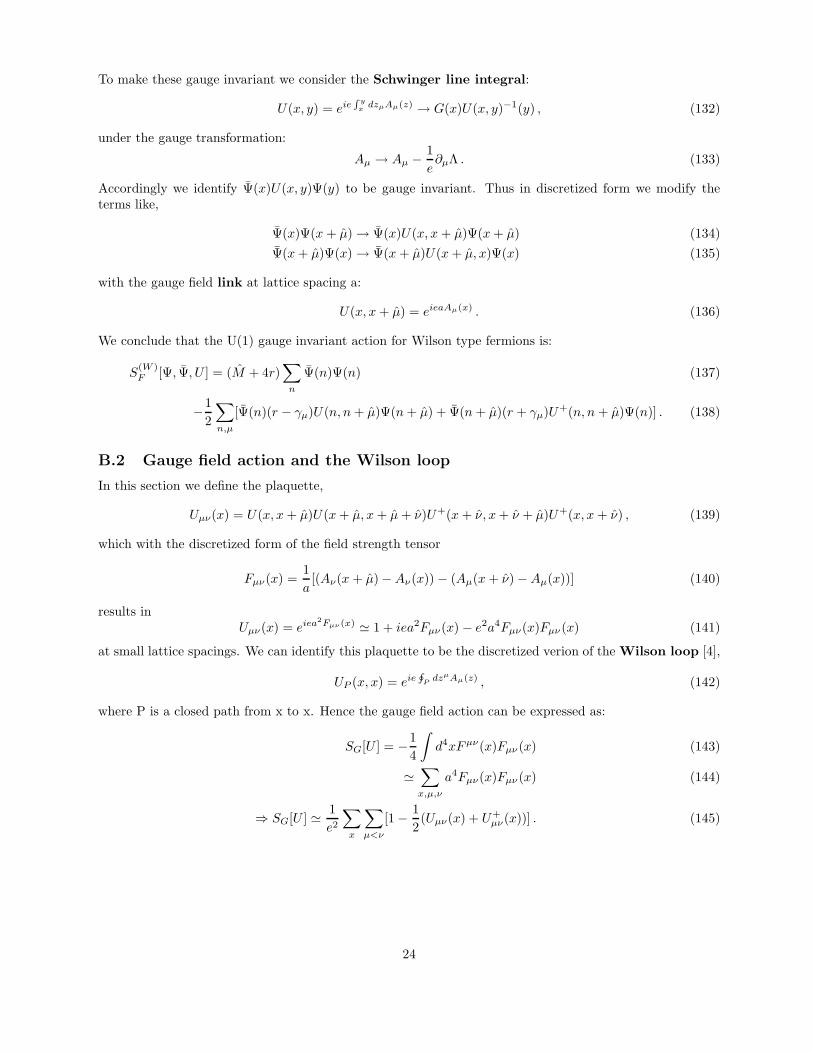
B.2 Gauge field action and the Wilson loop

In this section we define the plaquette,

Uµν(x) = U(x, x+ µ)U(x+ µ, x+ µ+ ν)U+(x+ ν, x+ ν + µ)U+(x, x + ν) , (139)

which with the discretized form of the field strength tensor

Fµν(x) =1

a[(Aν(x + µ) −Aν(x)) − (Aµ(x+ ν) −Aµ(x))] (140)

results inUµν(x) = eiea2Fµν(x) ≃ 1 + iea2Fµν(x) − e2a4Fµν(x)Fµν(x) (141)

at small lattice spacings. We can identify this plaquette to be the discretized verion of the Wilson loop [4],

UP (x, x) = eieH

PdzµAµ(z) , (142)

where P is a closed path from x to x. Hence the gauge field action can be expressed as:

SG[U ] = −1

4

∫

d4xFµν(x)Fµν(x) (143)

≃∑

x,µ,ν

a4Fµν(x)Fµν(x) (144)

⇒ SG[U ] ≃ 1

e2

∑

x

∑

µ<ν

[1 − 1

2(Uµν(x) + U+

µν(x))] . (145)

24

B.3 Non-Abelian gauge fields on the lattice

Let us now generalize the case of the U(1) gauge symmetry to the case of the non-Abelian unitary groupSU(N). Therefore we introduce N-component spinor fields,

~Ψ =

Ψ1

Ψ2

Ψ3

.

.

.ΨN

, ~Ψ =(

Ψ1, Ψ2, Ψ3, . . . , ΨN)

(146)

transforming in analogy to the Abelian case as,

~Ψ(x) → G(x)~Ψ(x) (147)

~Ψ(x) → ~Ψ(x)G−1(x) (148)

(149)

where now G(x) is an element of the fundamental representation of the group SU(N).Then the link variables are simply replaced by matrices in colour space:

U(x, x+ µ) = eig0aAµ(x) . (150)

With these replacements we retain the same form of the action for Wilson fermions. However as the gaugefield action in the continuum, which is

SG =1

2Tr

∫

d4xFµνFµν =1

4

∫

d4xFBµνF

Bµν , (151)

now contains a trace over the matrix valued field strength, we also obtain obtain a matrix for the case ofthe Wilson plaquette.

Uµν(x) = eig0a2Fµν(x) (152)

One can explicitly show that also in matrix representation

SG =2

g20

Tr∑

x

∑

µ<ν

[1 − 1

2(Uµν(x) + U+

µν(x))] (153)

again gives the right continuum limit.

25

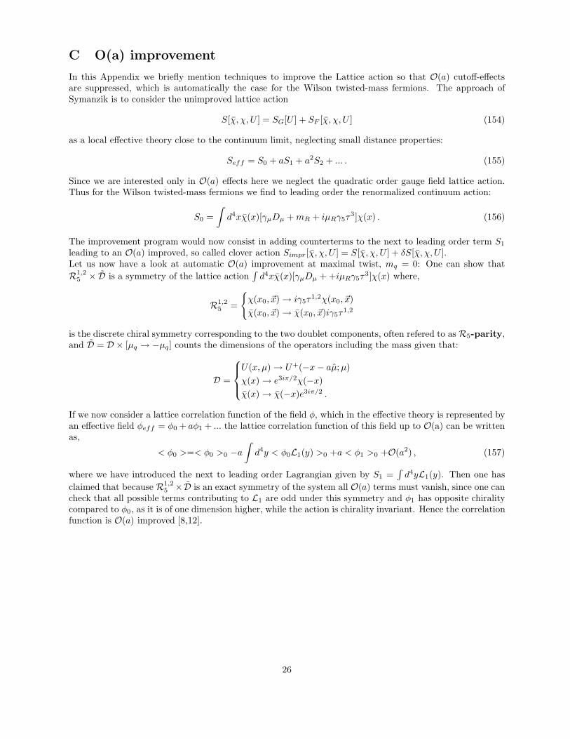
C O(a) improvement

In this Appendix we briefly mention techniques to improve the Lattice action so that O(a) cutoff-effectsare suppressed, which is automatically the case for the Wilson twisted-mass fermions. The approach ofSymanzik is to consider the unimproved lattice action

S[χ, χ, U ] = SG[U ] + SF [χ, χ, U ] (154)

as a local effective theory close to the continuum limit, neglecting small distance properties:

Seff = S0 + aS1 + a2S2 + ... . (155)

Since we are interested only in O(a) effects here we neglect the quadratic order gauge field lattice action.Thus for the Wilson twisted-mass fermions we find to leading order the renormalized continuum action:

S0 =

∫

d4xχ(x)[γµDµ +mR + iµRγ5τ3]χ(x) . (156)

The improvement program would now consist in adding counterterms to the next to leading order term S1

leading to an O(a) improved, so called clover action Simpr [χ, χ, U ] = S[χ, χ, U ] + δS[χ, χ, U ].Let us now have a look at automatic O(a) improvement at maximal twist, mq = 0: One can show that

R1,25 × D is a symmetry of the lattice action

∫

d4xχ(x)[γµDµ + +iµRγ5τ3]χ(x) where,

R1,25 =

χ(x0, ~x) → iγ5τ1,2χ(x0, ~x)

χ(x0, ~x) → χ(x0, ~x)iγ5τ1,2

is the discrete chiral symmetry corresponding to the two doublet components, often refered to as R5-parity,and D = D × [µq → −µq] counts the dimensions of the operators including the mass given that:

D =

U(x, µ) → U+(−x− aµ;µ)

χ(x) → e3iπ/2χ(−x)χ(x) → χ(−x)e3iπ/2 .

If we now consider a lattice correlation function of the field φ, which in the effective theory is represented byan effective field φeff = φ0 + aφ1 + ... the lattice correlation function of this field up to O(a) can be writtenas,

< φ0 >=< φ0 >0 −a∫

d4y < φ0L1(y) >0 +a < φ1 >0 +O(a2) , (157)

where we have introduced the next to leading order Lagrangian given by S1 =∫

d4yL1(y). Then one has

claimed that because R1,25 ×D is an exact symmetry of the system all O(a) terms must vanish, since one can

check that all possible terms contributing to L1 are odd under this symmetry and φ1 has opposite chiralitycompared to φ0, as it is of one dimension higher, while the action is chirality invariant. Hence the correlationfunction is O(a) improved [8,12].

26

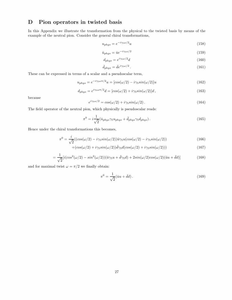
D Pion operators in twisted basis

In this Appendix we illustrate the transformation from the physical to the twisted basis by means of theexample of the neutral pion. Consider the general chiral transformations,

uphys = e−iγ5ω/2u (158)

uphys = ue−iγ5ω/2 (159)

dphys = eiγ5ω/2d (160)

dphys = deiγ5ω/2 . (161)

These can be expressed in terms of a scalar and a pseudoscalar term,

uphys = e−iγ5ωπ/2u = [cos(ω/2) − iγ5sin(ω/2)]u (162)

dphys = eiγ5ωπ/2d = [cos(ω/2) + iγ5sin(ω/2)]d , (163)

becauseeiγ5ω/2 = cos(ω/2) + iγ5sin(ω/2) . (164)

The field operator of the neutral pion, which physically is pseudoscalar reads:

π0 = i1√2(uphysγ5uphys + dphysγ5dphys) . (165)

Hence under the chiral transformations this becomes,

π0 =i√2((cos(ω/2) − iγ5sin(ω/2))uγ5u(cos(ω/2) − iγ5sin(ω/2)) (166)

+(cos(ω/2) + iγ5sin(ω/2))dγ5d(cos(ω/2) + iγ5sin(ω/2))) (167)

=1√2[i(cos2(ω/2) − sin2(ω/2))(uγ5u+ dγ5d) + 2sin(ω/2)cos(ω/2)(uu+ dd)] (168)

and for maximal twist ω = π/2 we finally obtain:

π0 =1√2(uu+ dd) . (169)

27

References

[1] M. Creutz and B. Freedman, “A Statistical Approach To Quantum Mechanics”Annals Phys. 132, 427 (1981)

[2] H. J. Rothe, “Lattice gauge theories: An Introduction” World Sci. Lect. Notes Phys. 74 (2005)

[3] T. DeGrand and C. E. Detar, “Lattice methods for quantum chromodynamics”New Jersey, USA: World Scientific (2006) 345 p

[4] M. E. Peskin and D. V. Schroeder, “An Introduction To Quantum Field Theory”Reading, USA: Addison-Wesley (1995) 842 p

[5] Ph. Boucaud et al. [ETM collaboration], “Dynamical Twisted Mass Fermions with Light Quarks:Simulation and Analysis Details”Comput. Phys. Commun. 179 (2008) 695 [arXiv:0803.0224 [hep-lat]].

[6] K. Jansen, C. McNeile, C. Michael, C. Urbach and f. t. E. Collaboration, “Meson masses and decayconstants from unquenched lattice QCD” arXiv:0906.4720 [hep-lat].

[7] K. Jansen, C. Michael and C. Urbach [ETM Collaboration], “The eta’ meson from lattice QCD”Eur. Phys. J. C 58 (2008) 261 [arXiv:0804.3871 [hep-lat]].

[8] R. Frezzotti and G. C. Rossi, “Chirally improving Wilson fermions. I: O(a) improvement”JHEP 0408, 007 (2004) [arXiv:hep-lat/0306014].

[9] U. Wolff [ALPHA collaboration], “Monte Carlo errors with less errors”Comput. Phys. Commun. 156 (2004) 143 [Erratum-ibid. 176 (2007) 383] [arXiv:hep-lat/0306017].

[10] P. A. Boyle, A. Juttner, C. Kelly and R. D. Kenway, “Use of stochastic sources for the lattice deter-mination of light quark physics” JHEP 0808 (2008) 086 [arXiv:0804.1501 [hep-lat]]

[11] B. Efron and Robert. J. Tibshirani, “An introduction to the bootstrap”Boca Raton, USA: Chapman and Hall/CRC (1993)

[12] A. Shindler, “Twisted mass lattice QCD” Phys. Rept. 461 (2008) 37 [arXiv:0707.4093 [hep-lat]]

[13] A. M. Sanchez, R. Welsing “Looking at the Harmonic Oscillator with Lattice field theoretical methods”DESY Summer Student Programme (2008)[http://www-zeuthen.desy.de/summerstudents/2008/doc/Welsing.pdf]

28