Computation of continuous and piecewise affine Lyapunov functions bynumerical approximations of the Massera construction

Johann Bjornsson1, Peter Giesl2, Sigurdur Hafstein1, Christopher M. Kellett3, and Huijuan Li4

Abstract— The numerical construction of Lyapunov functionsprovides useful information on system behavior. In the Contin-uous and Piecewise Affine (CPA) method, linear programmingis used to compute a CPA Lyapunov function for continuousnonlinear systems. This method is relatively slow due to thelinear program that has to be solved. A recent proposal wasto compute the CPA Lyapunov function based on a Lyapunovfunction in a converse Lyapunov theorem by Yoshizawa. Inthis paper we propose computing CPA Lyapunov functionsusing a Lyapunov function construction in a classic converseLyapunov theorem by Massera. We provide the theory for sucha computation and present several examples to illustrate theutility of this approach.

I. INTRODUCTION

Let K ⊂ Rn be a compact neighborhood of the originand consider a C2 vector field f : K → Rn. We consider adynamical system

x = f(x) (I.1)

where the origin is an asymptotically stable equilibriumpoint. As the general reader will be well aware, it can bedifficult to find the general solution to such a system, thatis for a given x ∈ K and an interval I ⊂ R≥0 finda function φ : I × Rn → Rn such that d

dtφ(t,x) =f(φ(t,x)), φ(0,x) = x. Our goal then instead is to constructa continuous Lyapunov function for the system, that is apositive definite continuous function V : K → R suchthat for every solution φ of d

dtφ(t,x) = f(φ(t,x)) onK \ {0} we have for every t0, t1 ∈ I that t0 < t1 impliesV (φ(t0,x)) < V (φ(t1,x)). It is well known that thiscondition follows for a Lipschitz V such that

V +(x) := lim suph→0+

V (x + hf(x))− V (x)h

< 0

on K◦ where K◦ denotes the interior of the set K ⊂ Rn.Note that V +(x) is sometimes referred to as the orbitalderivative of V at x with respect to f ; or simply the orbitalderivative of V .

In general, constructing a Lyapunov function for (I.1) is adifficult problem. However, once constructed on a specific

1J. Bjornsson (johannsb13@ru.is) and S. Hafstein (sigurdurh@ru.is) arewith the School of Science and Engineering, Reykjavik University, Iceland.Bjornsson is supported by The Icelandic Research Fund, grant nr. 130677-052. 2P. Giesl is with the Department of Mathematics, University of Sussex,UK. 3C.M. Kellett (Chris.Kellett@newcastle.edu.au) is with the School ofElectrical Engineering and Computer Science, University of Newcastle,Callaghan, New South Wales, Australia. Kellett is supported by ARCFuture Fellowship FT1101000746 and by the Alexander von HumboldtFoundation. 4 H. Li (Huijuan.Li@uni-bayreuth.de) is with the Departmentof Mathematics, University of Bayreuth, Germany. Li is supported by the EUInitial Training Network “Sensitivity Analysis for Deterministic ControllerDesign-SADCO”.

domain, a Lyapunov function gives a good idea of thebehavior of all solutions in that domain. In particular, itssublevel sets are inner bounds on the basin of attraction ofthe equilibrium.

There have been numerous proposals of how to computeLyapunov functions numerically for nonlinear systems. Forexample, collocation methods were proposed in [11], [3],[21], graph theoretic methods in [2], [12], semidefiniteoptimization for sum-of-squares polynomials (SOS method)[17], [18], [19], as well as automated algebraic methods [20],[22].

In [15] a method was proposed for constructing a Lya-punov function by solving linear inequalities on a finiteset of points in K, called a vertex set for K, which inturn determine a unique continuous piecewise affine (CPA)Lyapunov function on the whole of K. This method isreferred to as the CPA method. The CPA method has beenimproved [7] and extended to different kinds of systems [9],[1], [5], [6].

The method presented here is a simple modification of theCPA method where, instead of using linear programmingto determine the values at the points of the vertex set,we use a function construction from a classical converseLyapunov theorem developed by Massera [16] to determinethe values. This is similar to the procedure in [10] where aconstruction due to Yoshizawa [25] was used. As with theYoshizawa construction, the complexity of the computationfor the Massera construction used herein is linear in thenumber of grid points and is thus much lower than whenthe linear programming is used. A theoretical advantage ofthe Massera construction to the Yoshizawa construction isthat the Lyapunov function is guaranteed to be as smooth asthe vector field f in (I.1).

This paper is organized as follows. In Section II we give abrief summary of the CPA method and describe the converseLyapunov theorem that provides the function we use to definea CPA function. In Section III we present four numericalexamples illustrating the utility of our proposed construction.

We denote the positive integers by N and the strictly posi-tive real numbers by R>0. For a vector x = [x1, . . . , xn]T ∈Rn we define the norms ‖x‖p = (

∑ni=1 |xi|p)

1p for p ≥ 1

and denote for a set A ⊆ Rn its diameter by diam2(A) :=supx,y∈A ‖x−y‖2. We denote the open ball in Rn of radiusr > 0 centered at the origin by

Br := {x ∈ Rn : ‖x‖2 < r}.

II. THEORY

We start by giving a summary of the CPA method aspresented in [9]. We define a grid on K ⊂ Rn and calculatefor each point x in the grid the value that V is to take atx. The values for V on the grid can then be used to extendV to all of K such that V is a continuous piecewise affineLyapunov function on K. In this section we shall providethe details of this construction.

Let x0, . . . ,xk be a collection of affinely independentpoints in Rn, that is

∑ki=0 ci(xi−x0) = 0 implies that ci =

0 for i = 1, . . . , k. The convex combination of x0, . . . ,xk,that is the set co{x0, . . . ,xk} := {

∑ki=0 cixi | all ci ≥

0 and∑ki=0 ci = 1}, is a k-simplex in Rn.

Let T = {T1, . . . , Tm} be a set of k-simplices such thatK = ∪mi=1Ti. Suppose further that for every i, j such that i 6=j we have that Ti∩Tj = ∅ or that Ti∩Tj is an h-simplex withh < k. We then say that T is a triangulation of K. We furtherdefine VT := {x ∈ Rn |x is a vertex of a simplex in T }and call VT the vertex set for the triangulation.

For a given triangulation T = {T1, . . . , Tm} and afunction V0 : VT → R we can uniquely extend V0 to acontinuous piecewise affine function V : K → R that is C∞

in the interior of each simplex Ti. More specifically:i) If x ∈ VT then V (x) = V0(x).

ii) For every Ti ∈ T there exists a linear mapping Ai :Rn → R and bi ∈ R such that V (x) = Ai(x) + bi forall x ∈ Ti and such that V is continuous on K.

We are interested in systems (I.1) with an asymptoticallystable equilibrium at the origin and consequently in Lya-punov functions with a minimum at the origin. Since a localminimum for a CPA function can only be attained at a vertex,we insist that the origin be a vertex of our triangulation.For a given triangulation T of K we denote the collectionof all continuous piecewise affine functions as describedabove by CPA[T ] and identify each such function with thecorresponding function V0 : VT → R by V ∼ (V0(x))x∈VT .

The following theorem from [9] states that in order toconstruct a Lyapunov function for (I.1) it is sufficient todetermine a function V0 : VT → R which satisfies certaininequalities at each vertex x ∈ VT , for then the CPAinterpolation of V0 on K is a CPA Lyapunov function for(I.1) on the whole of K.

Theorem 2.1: Consider the system (I.1) with triangulationT = {T1, . . . , Tm}. Let V ∼ (V0(x))x∈VT ∈ CPA[T ]. Foreach Ti ∈ T define the constants hi := diam2(Ti) and

Ei :=nMi

2h2i , where (II.1)

Mi ≥ maxm,r,s=1,2,...,n

maxz∈Ti

∣∣∣∣ ∂2fm∂xr∂xs

(z)∣∣∣∣ .

Assume that for a simplex Ti = co{x0,x1, . . . ,xk} ∈ T theinequality

∇Vi · f(xj) + Ei‖∇Vi‖1 < 0 (II.2)

holds true for every vertex xj ∈ Ti. Then

∇Vi · f(x) < 0 for all x ∈ Ti.

If the inequality (II.2) holds true for Ti1 , Ti2 , . . . , Tim , wehave V +(x) < 0 for all x ∈ (∪mj=1Tij )◦.Note that the constants Ei are upper bounds and one does nothave to compute them exactly. A rough estimate is sufficientand easily obtainable in practice.

In [9] the values of V0 at the vertex points are determinedby linear programming. Here we propose a different, andmuch faster, method to calculate the vertex values similarto the one described in [10]. In [16] Massera proved a con-verse Lyapunov theorem for systems with an asymptoticallystable equilibrium at the origin by constructing a Lyapunovfunction based on the integral of a nonlinear scaling of thenorm of the state trajectory. While Massera’s constructionis applicable to asymptotic stability, for simplicity we hereassume exponential stability. The following formulation is aslightly simplified version of [14, Theorem 4.14].

Theorem 2.2: Consider a dynamical system x = f(x)where f is C2 on Br ⊂ Rn for some r ∈ R>0 and supposethat 0 is an exponentially stable equilibrium point for thesystem, that is there exist constants k, λ ∈ R>0 such that‖φ(t,x)‖ ≤ k‖x‖e−λt for all t ≥ 0 such that x ∈ Br. Thenthere exists a constant N such that

V (x) :=∫ N

0

‖φ(τ,x)‖2dτ. (II.3)

is a Lyapunov function for the system on Br.As indicated in [14] the constant N can be taken to be

N = ln(2k2)2λ . However, since it can be difficult to determine

λ and k for specific systems this equation is of limitedpractical value. It is also worth noting that the functionconstructed in Theorem 2.2 inherits the smoothness attributesof f , essentially because φ does (c.f., [24, p. 157]), so wehave V ∈ C2(Br \ {0}).

To generalize the above to asymptotically stable systemswe can take a nonlinear scaling of the norm of the statetrajectory obtained from a class-KL asymptotic stability esti-mate and Sontag’s Lemma on KL-estimates [23, Proposition7] (also [13, Lemma 7]) which provides an exponentiallydecreasing in time upper bound for the asymptotic stabilityestimate (see [13] for the definition of class-KL).

Our modification of the CPA method is the following:1) For a given compact neighborhood K ⊂ Rn of the

origin, define a sequence (Tj)j∈N of triangulations ofK that have uniformly bounded degeneracy (for details,cf. [1, Remark 4.7] or the discussion after [10, Defini-tion 3]) and such that

limj→∞

(maxT∈Tj

diam2(T ))

= 0.

2) Fix an increasing function g : N → R>0 withlimj→∞ g(j) =∞.

3) Set j = 1.4) Compute

V j0 (x) =∫ g(j)

0

‖φ(τ,x)‖2dτ (II.4)

at the vertices VTj and by a convex interpolation con-struct a CPA function V j(x) on K.

5) Check inequality (II.2) at each vertex to determinewhere the CPA function V j(x) is a Lyapunov functionfor (I.1). If a finer result is required, increment j andreturn to Step 4. Otherwise stop.

By our choice of g it is obvious that g(j) > ln(2k2)2λ in the

long run, and in [8] and [10] it is demonstrated that thereexists a value δ > 0 such that if max

T∈Tdiam2(T ) < δ then the

Lyapunov function constructed by the CPA method in factsatisfies inequality (II.2) at every vertex point. Therefore,if K is in the basin of attraction of the equilibrium, anda priori given an arbitrary small ε-ball Bε centered at theorigin, the functions V j will be Lyapunov functions forthe system on K \ Bε for all large enough j. For all butthe most simple systems one has to approximate the valuesof V0 numerically. It is a matter of ongoing research howthis affects the inequalities at the vertices, but the numericalexamples presented below are promising.

III. EXAMPLES

In this section we present numerical examples that demon-strate the effectiveness of our modified CPA method. In whatfollows we use the classical Runge-Kutta method RK4 toapproximate φ(t,x). Across the examples, various step-sizes∆t for RK4 were used and for Examples 1-3 ∆t = 0.01was found to be sufficiently small. For Example 4 a smallerstep-size of ∆t = 0.001 yielded better results in terms ofobtaining a negative orbital derivative on more simplices.

In the following examples we set g(j) = 2j · 50 · ∆tand Sj = 4j · 200 for all j ∈ N where Sj denotes thenumber of simplices in our triangulation in the j-th stepof the algorithm. In other words, at each iteration of thealgorithm we double the upper limit of integration in (II.4)and have a fourfold increase in the number of simplices.

In the following figures we plot the calculated CPAfunction at a specific iteration of the algorithm and mark with∗ the simplices in which the computed CPA function fails tohave a negative orbital derivative. It is also worth noting thatall the functions we have calculated have been normalizedsuch that the maximum value of the CPA Lyapunov functionon its domain of definition is 1.

Example 1

Our first example is the linear system

x = Ax =[

1 1−5 −3

]x.

Since the eigenvalues of A are −1 + i and −1 − i thissystem has an exponentially stable equilibrium at the origin.We now utilize the modified CPA method proposed above tocalculate a Lyapunov function for the system on B1 and notethat, for linear systems, we can take Mi = 0, and hence weset Ei = 0 for each simplex. We plot the function given bythe first two iterations of the algorithm in Figures 1 and 2.Note that even two iterations yield a Lyapunov function onnearly the entire domain for the system. In Figure 3 we plotsome level curves for the CPA Lyapunov function obtainedon the third iteration. In Table I we give two measures for

Iteration Percentage of Simplices Radius (R) Outsidewith D+V (x) < 0 Which D+V < 0

1 91.750% 12 98.813% 6.25 · 10−2

3 99.719% 1.563 · 10−2

4 99.930% 3.91 · 10−3

5 99.982% 9.8 · 10−4

6 99.996% 2.4 · 10−4

TABLE ITWO DIFFERENT MEASURES FOR THE QUALITY OF THE COMPUTED CPALYAPUNOV FUNCTIONS FOR THE DIFFERENT ITERATIONS. IN COLUMN 2WE GIVE THE PERCENT OF THE NUMBER OF TRIANGLES Ti ∈ T , WHERE

THE ORBITAL DERIVATIVE D+V IS NEGATIVE AND IN COLUMN 3 WE

GIVE THE RADIUS R OF A BALL BR , OUTSIDE OF WHICH THE ORBITAL

DERIVATIVE IS NEGATIVE.

Fig. 1.First iteration of the algorithm for the system in Example

1. We obtain a CPA Lyapunov function for the system withnegative orbital derivative in 734 of the 800 simplices in

the triangulation.

the quality of the CPA Lyapunov functions computed in thedifferent iterations.

Example 2

Our next example is the non-linear system

x1 = −x2 − (1− x21 − x2

2)x1

x2 = x1 − (1− x21 − x2

2)x2.

By using polar coordinates or by linearizing one candemonstrate that the origin is exponentially stable. It is alsosimple to show that the unit circle is a recurrent set in thisexample, therefore it is prudent to utilize our method ona set slightly smaller than B1. We choose the set B0.95. Inthis example we set Ei = 6h2

i ·maxx∈Ti{|x1|, |x2|} for eachsimplex Ti and we obtain a Lyapunov function on the firstiteration, so further iterations are unnecessary. The resultingCPA Lyapunov function is displayed in Figure 4. By usinga slightly stricter version of Theorem 2.1 (cf. [4, Theorem2.6]), we can even assure that the CPA Lyapunov functionhas a negative orbital derivative on its entire domain, evenin a neighborhood of the origin.

In Figure 5 we plot some of its level curves.

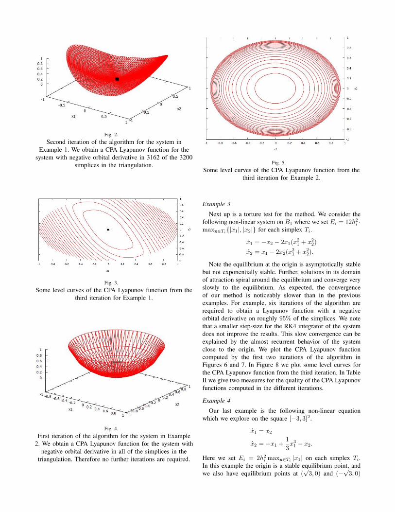
Fig. 2.Second iteration of the algorithm for the system in

Example 1. We obtain a CPA Lyapunov function for thesystem with negative orbital derivative in 3162 of the 3200

simplices in the triangulation.

Fig. 3.Some level curves of the CPA Lyapunov function from the

third iteration for Example 1.

Fig. 4.First iteration of the algorithm for the system in Example

2. We obtain a CPA Lyapunov function for the system withnegative orbital derivative in all of the simplices in the

triangulation. Therefore no further iterations are required.

Fig. 5.Some level curves of the CPA Lyapunov function from the

third iteration for Example 2.

Example 3

Next up is a torture test for the method. We consider thefollowing non-linear system on B1 where we set Ei = 12h2

i ·maxx∈Ti

{|x1|, |x2|} for each simplex Ti.

x1 = −x2 − 2x1(x21 + x2

2)

x2 = x1 − 2x2(x21 + x2

2).

Note the equilibrium at the origin is asymptotically stablebut not exponentially stable. Further, solutions in its domainof attraction spiral around the equilibrium and converge veryslowly to the equilibrium. As expected, the convergenceof our method is noticeably slower than in the previousexamples. For example, six iterations of the algorithm arerequired to obtain a Lyapunov function with a negativeorbital derivative on roughly 95% of the simplices. We notethat a smaller step-size for the RK4 integrator of the systemdoes not improve the results. This slow convergence can beexplained by the almost recurrent behavior of the systemclose to the origin. We plot the CPA Lyapunov functioncomputed by the first two iterations of the algorithm inFigures 6 and 7. In Figure 8 we plot some level curves forthe CPA Lyapunov function from the third iteration. In TableII we give two measures for the quality of the CPA Lyapunovfunctions computed in the different iterations.

Example 4

Our last example is the following non-linear equationwhich we explore on the square [−3, 3]2.

x1 = x2

x2 = −x1 +13x3

1 − x2.

Here we set Ei = 2h2i maxx∈Ti

|x1| on each simplex Ti.In this example the origin is a stable equilibrium point, andwe also have equilibrium points at (

√3, 0) and (−

√3, 0)

Fig. 6.First iteration of the algorithm for the system in Example

3. We obtain a CPA Lyapunov function for the system withnegative orbital derivative in 632 of the 800 simplices in

the triangulation.

Fig. 7.Second iteration of the algorithm for the system in

Example 3. We obtain a CPA Lyapunov function for thesystem with negative orbital derivative in 2680 of the 3200

simplices in the triangulation.

Fig. 8.Some level curves of the CPA Lyapunov function from the

third iteration for Example 3.

Iteration Percentage of Simplices Radius (R) Outsidewith D+V (x) < 0 Which D+V < 0

1 79.000% 0.250002 83.750% 0.202503 88.031% 0.140634 90.930% 0.105635 93.205% 0.075636 94.833% 0.05790

TABLE IITWO DIFFERENT MEASURES FOR THE QUALITY OF THE COMPUTED CPALYAPUNOV FUNCTIONS IN EXAMPLE 3 FOR DIFFERENT ITERATIONS. IN

COLUMN 2 WE GIVE THE PERCENT OF THE NUMBER OF TRIANGLES

Ti ∈ T , WHERE THE ORBITAL DERIVATIVE D+V IS NEGATIVE AND IN

COLUMN 3 WE GIVE THE RADIUS R OF A BALL BR , OUTSIDE OF WHICH

THE ORBITAL DERIVATIVE IS NEGATIVE.

Fig. 9.First iteration of the algorithm for the system in Example

4. We obtain a CPA Lyapunov function for the system withnegative orbital derivative in 644 of the 800 simplices in

the triangulation.

that are unstable. Therefore we cannot expect to obtain aLyapunov function on the whole square, but as an interestingapplication we note that the domain in which we obtain aLyapunov function for the system gives a rough estimateof the basin of attraction for the stable equilibrium pointat the origin (cf. Figure 11). We plot the CPA Lyapunovfunction computed by the first two iterations of the algorithmin Figures 9 and 10. In Figure 11 we plot some level curvesfor the CPA Lyapunov function from the third iteration.

IV. CONCLUSIONS

We have proposed a modified CPA method for the con-struction of Lyapunov functions on compact regions con-taining the origin using a classical Lyapunov function con-struction due to Massera. This modification has the benefitthat computation of the vertex values for the candidateCPA Lyapunov function is much faster than the solving thelinear program necessary for the original CPA method [15].We presented several numerical examples demonstrating theutility of this modified CPA method.

Fig. 10.Second iteration of the algorithm for the system in example4. We obtain a CPA Lyapunov function for the system withnegative orbital derivative in 2598 of the 3200 simplices in

the triangulation.

Fig. 11.Some level curves of the CPA Lyapunov function from the

third iteration for Example 4.

While (II.3) is known to be a Lyapunov function, the sys-tem trajectories obtained via the Runge–Kutta RK4 methodare obviously an approximation. This causes no difficulty aswe may, in fact, choose any values for the vertices to thendefine the candidate CPA Lyapunov function and then useTheorem 2.1 to determine whether or not those particularvertex values do, in fact, yield a negative orbital derivativeon each simplex. Using approximate values of (II.3) to fixthe vertex values is then, in some sense, a principled guesssince the results of [8] and [10] guarantee that, by a processof iteratively refining the triangulation, using exact values of(II.3) will eventually yield a CPA Lyapunov function.

REFERENCES

[1] R. Baier, L. Grune, and S. Hafstein. Linear programming basedLyapunov function computation for differential inclusions. Discreteand Continuous Dynamical Systems Series B, 17:33–56, 2012.

[2] H. Ban and W. Kalies. A computational approach to Conley’sdecomposition theorem. Journal of Computational and NonlinearDynamics, 1-4:312–319, 2006.

[3] P. Giesl. Construction of Global Lyapunov Functions Using RadialBasis Functions. Number 1904 in Lecture Notes in Mathematics.Springer, 2007.

[4] P. Giesl and S. Hafstein. Construction of Lyapunov functions fornonlinear planar systems by linear programming. J. Math. Anal. Appl.,388:463–479, 2012.

[5] P. Giesl and S. Hafstein. Construction of a CPA contraction metric forperiodic orbits using semidefinite optimization. Nonlinear Analysis:Theory, Methods & Applications, 86:114–134, 2013.

[6] P. Giesl and S. Hafstein. Computation of Lyapunov functions fornonlinear discrete time systems by linear programming. J. Dif-fer. Equ. Appl., 2014.

[7] P. Giesl and S. Hafstein. Revised CPA method to compute Lyapunovfunctions for nonlinear systems. J. Math. Anal. Appl., 410:292–306,2014.

[8] S. Hafstein. A constructive converse Lyapunov theorem on exponentialstability. Discrete Contin. Dyn. Syst., 10(3):657–678, 2004.

[9] S. Hafstein. An Algorithm for Constructing Lyapunov Functions.Electronic Journal of Differential Equations Mongraphs, 2007.

[10] S. Hafstein, C. M. Kellett, and H. Li. Continuous and piecewise affineLyapunov functions using the Yoshizawa construction. In Proceedingsof the American Control Conference, 2014.

[11] T. Johansen. Computation of Lyapunov functions for smooth nonlinearsystems using convex optimization. Automatica, 36:1617–1626, 2000.

[12] W. Kalies, K. Mischaikow, and R. VanderVorst. An algorithmicapproach to chain recurrence. Foundations of Computational Mathe-matics, 5-4:409–449, 2005.

[13] C. M. Kellett. A compendium of comparsion function results.Mathematics of Controls, Signals and Systems, 26(3):339–374, 2014.

[14] H. K. Khalil. Nonlinear Systems. Prentice Hall, 3 edition, 2002.[15] S. Marinosson. Lyapunov function construction for ordinary differen-

tial equations with linear programming. Dynamical Systems, 17:137–150, 2002.

[16] J. L. Massera. On Liapounoff’s conditions of stability. Annals ofMathematics, 50:705–721, 1949.

[17] A. Papachristodoulou and S. Prajna. The construction of Lyapunovfunctions using the sum of squares decomposition. In Proceedings ofthe 41st IEEE Conference on Decision and Control, pages 3482–3487,2002.

[18] M. Peet. Exponentially stable nonlinear systems have polynomialLyapunov functions on bounded regions. IEEE Trans. AutomaticControl, 54:979–987, 2009.

[19] M. Peet and A. Papachristodoulou. A converse sum-of-squaresLyapunov result: An existence proof based on the Picard iteration. InProceedings of the 49th IEEE Conference on Decision and Control,pages 5949–5954, 2010.

[20] S. Ratschan and Z. She. Providing a basin of attraction to atarget region of polynomial systems by computation of Lyapunov-like functions. SIAM J. Control and Optimization, 48(7):4377–4394,2010.

[21] M. Rezaiee-Pajand and B. Moghaddasie. Estimating the regionof attraction via collocation for autonomous nonlinear systems.Struct. Eng. Mech., 41(2):263–284, 2012.

[22] Z. She, H. Li, B. Xue, Z. Zheng, and B. Xia. Discovering polynomialLyapunov functions for continuous dynamical systems. J. Symb. Com-put., 58:41–63, 2013.

[23] E. D. Sontag. Comments on integral variants of ISS. Systems andControl Letters, 34(1–2):93–100, 1998.

[24] W. Walter. Ordinary Differential Equations. Springer, 1998. Translatedfrom the German by R. Thompson.

[25] T. Yoshizawa. Stability Theory by Liapunov’s Second Method. Math-ematical Society of Japan, 1966.