Computaonal&Physics&I Project...

Prof. Alexander Knebe

Computa5onal Physics I Project

rules and regula+ons

!  project:

"  you can pick one of the projects from the lists provided below or...

"  you can write a short project proposal where you explain and specify: •  the project itself…

o  what is the physical problem (equa5ons!)?

o  what are your objec5ves, what do you plan to do? o  list of order 4-‐6 milestones

•  arrange and discuss the project and the milestones with your teacher

!  project report:

"  you have to write a report that summarizes your work and the results

•  present your results and conclusions

•  elaborate on the objec5ves and your milestones

!  presenta.on:

"  you have to orally present the results of your project in class: •  10min. presenta5on + 2 min. ques5ons from fellow students (and teacher)

!  distribu.on of points:

•  quality of project realisa5on 4 points •  quality of MATLAB script(s) 3 points •  project report 2 point •  presenta5on of results 1 points

!  Note: you need to work in teams of 2 students!


quality guidelines

!  project:

"  the project is not an exam:

•  you should study and inves+gate a physical problem!

•  if you picked one of the suggested projects, the listed objec6ves and milestones are just a guideline: simply presen6ng plots for the listed milestones will let you pass the project, but not obtain the highest possible mark: it is certainly necessary to add even more milestones depending on your interests…

•  if you chose to select your own project, you need to have clear objec6ves in mind and synchronize/define all milestones with your teacher.

!  project report:

"  the report needs to feature an introduc.on, a results, and a summary part:

•  the introduc+on needs to explain (to a fellow student!) the idea/history of the project, the relevant equa6ons, and the theory behind the physical system in general

•  in the results part you need to show (key) plots from your inves6ga6on and discuss them; you do not need to show all plots generated during the inves6ga6on, but you need to explain clearly all results you found. The results part should be well structured primarily following your objec6ves and milestones

•  the summary part should contain a brief summary of the main findings and your conclusions about the physical system

!  presenta.on:

"  the presenta5on is structured similarly to the report: introduc5on, results & summary

"  the presenta5on should focus on explaining the project to your fellow students and showing key results from your study of it

"  the presenta5on is strictly 10 min. long; running over5me will make you loose points!

!  Notes:

"  MATLAB scripts are not allowed to appear in the report or the presenta5on



"  Feb 2nd: choice of project (or submission of proposal) to [email protected]

"  April 6st: submission of complete project: •  report describing your results and the milestones •  the script(s) used to generate the plots and/or results

"  April 16th & 17th: oral presenta5on of projects (10+2 minutes)

schedule for academic year 2017/18

project sugges+ons

you may pick a project from the provided list,

but you are encouraged to come up with a project on your own!

come and see me in C-‐8-‐316 if you have ques+ons and/or want to discuss your project!


−20

−15

−10

−5

0

5

10

15

20 −25

−20−15

−10−5

05

1015

20

25

0

5

10

15

20

25

30

35

40

45

50

y

deterministic chaos

x

z


example projects

€

dxdt

=σ(y − x)

dydt

= rx − y − xz

dzdt

= xy − bz

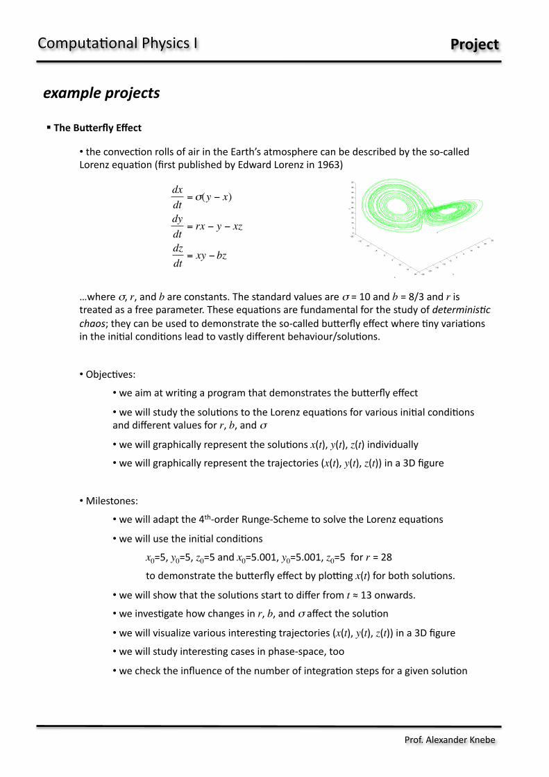
"  The Bu<erfly Effect

•  the convec5on rolls of air in the Earth’s atmosphere can be described by the so-‐called Lorenz equa5on (first published by Edward Lorenz in 1963)

…where σ, r, and b are constants. The standard values are σ = 10 and b = 8/3 and r is treated as a free parameter. These equa5ons are fundamental for the study of determinis6c chaos; they can be used to demonstrate the so-‐called buaerfly effect where 5ny varia5ons in the ini5al condi5ons lead to vastly different behaviour/solu5ons.

•  Objec5ves: •  we aim at wri5ng a program that demonstrates the buaerfly effect

•  we will study the solu5ons to the Lorenz equa5ons for various ini5al condi5ons and different values for r, b, and σ

•  we will graphically represent the solu5ons x(t), y(t), z(t) individually •  we will graphically represent the trajectories (x(t), y(t), z(t)) in a 3D figure

•  Milestones:

•  we will adapt the 4th-‐order Runge-‐Scheme to solve the Lorenz equa5ons

•  we will use the ini5al condi5ons x0=5, y0=5, z0=5 and x0=5.001, y0=5.001, z0=5 for r = 28 to demonstrate the buaerfly effect by ploing x(t) for both solu5ons.

•  we will show that the solu5ons start to differ from t ≈ 13 onwards. •  we inves5gate how changes in r, b, and σ affect the solu5on •  we will visualize various interes5ng trajectories (x(t), y(t), z(t)) in a 3D figure •  we will study interes5ng cases in phase-‐space, too •  we check the influence of the number of integra5on steps for a given solu5on


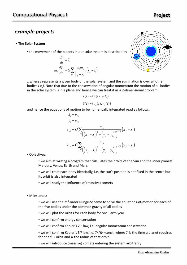
"  The Solar System

•  the movement of the planets in our solar system is described by

…where i represents a given body of the solar system and the summa5on is over all other bodies i ≠ j. Note that due to the conserva5on of angular momentum the mo5on of all bodies in the solar system is in a plane and hence we can treat it as a 2-‐dimensional problem:

and hence the equa5ons of mo5on to be numerically integrated read as follows:

•  Objec5ves: •  we aim at wri5ng a program that calculates the orbits of the Sun and the inner planets Mercury, Venus, Earth and Mars.

•  we will treat each body iden5cally, i.e. the sun’s posi5on is not fixed in the centre but its orbit is also integrated

•  we will study the influence of (massive) comets

•  Milestones:

•  we will use the 2nd-‐order Runge-‐Scheme to solve the equa5ons-‐of-‐mo5on for each of the five bodies under the common gravity of all bodies

•  we will plot the orbits for each body for one Earth year. •  we will confirm energy conserva5on

•  we will confirm Kepler’s 2nd law, i.e. angular momentum conserva5on

•  we will confirm Kepler’s 3rd law, i.e. T2/R3=const. where T is the 5me a planet requires for one full orbit and R the radius of that orbit. •  we will introduce (massive) comets entering the system arbitrarily


example projects

€

! r (t) = x(t), y(t)( )! v (t) = vx (t), vy (t)( )

€

d! r idt

=! v i

mid! v idt

= Gmim j! r j −! r i3! r j −! r i( )

j≠ i∑

€

˙ x i = vi,x

˙ y i = vi,y

˙ v i,x = Gm j

x j − xi( )2

+ y j − yi( )2#

$ % &

' (

3 / 2 x j − xi( )j≠ i∑

˙ v i,y = Gm j

x j − xi( )2

+ y j − yi( )2#

$ % &

' (

3 / 2 y j − yi( )j≠ i∑


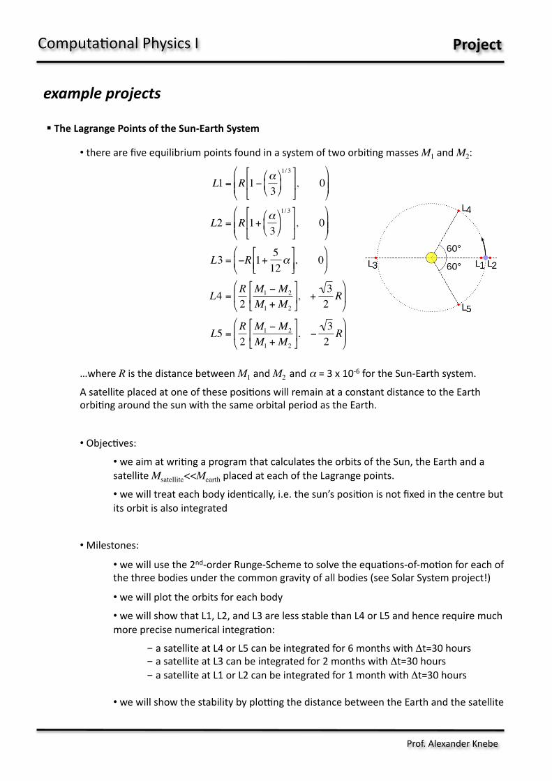
"  The Lagrange Points of the Sun-‐Earth System

•  there are five equilibrium points found in a system of two orbi5ng masses M1 and M2:

…where R is the distance between M1 and M2 and α = 3 x 10-‐6 for the Sun-‐Earth system.

A satellite placed at one of these posi5ons will remain at a constant distance to the Earth orbi5ng around the sun with the same orbital period as the Earth.

•  Objec5ves: •  we aim at wri5ng a program that calculates the orbits of the Sun, the Earth and a satellite Msatellite<<Mearth placed at each of the Lagrange points.

•  we will treat each body iden5cally, i.e. the sun’s posi5on is not fixed in the centre but its orbit is also integrated

•  Milestones:

•  we will use the 2nd-‐order Runge-‐Scheme to solve the equa5ons-‐of-‐mo5on for each of the three bodies under the common gravity of all bodies (see Solar System project!)

•  we will plot the orbits for each body •  we will show that L1, L2, and L3 are less stable than L4 or L5 and hence require much more precise numerical integra5on:

-  a satellite at L4 or L5 can be integrated for 6 months with Δt=30 hours -  a satellite at L3 can be integrated for 2 months with Δt=30 hours -  a satellite at L1 or L2 can be integrated for 1 month with Δt=30 hours

•  we will show the stability by ploing the distance between the Earth and the satellite


example projects

€

L1 = R 1− α3

$

% &

'

( ) 1/ 3*

+ ,

-

. / , 0

$

% & &

'

( ) )

L2 = R 1+α3

$

% &

'

( ) 1/ 3*

+ ,

-

. / , 0

$

% & &

'

( ) )

L3 = −R 1+512α

*

+ , -

. / , 0

$

% &

'

( )

L4 =R2

M1 −M2

M1 + M2

*

+ ,

-

. / , +

32R

$

% &

'

( )

L5 =R2

M1 −M2

M1 + M2

*

+ ,

-

. / , −

32R

$

% &

'

( )



example projects

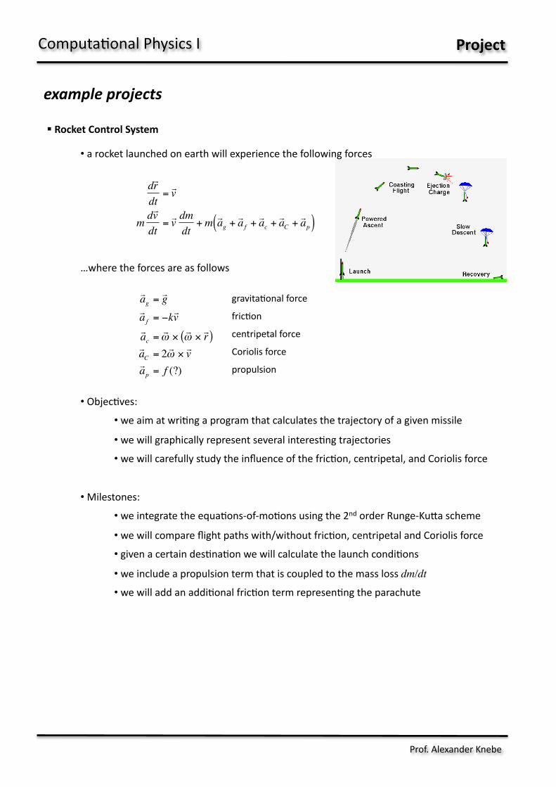
"  Rocket Control System

•  a rocket launched on earth will experience the following forces

…where the forces are as follows

•  Objec5ves: •  we aim at wri5ng a program that calculates the trajectory of a given missile

•  we will graphically represent several interes5ng trajectories •  we will carefully study the influence of the fric5on, centripetal, and Coriolis force

•  Milestones:

•  we integrate the equa5ons-‐of-‐mo5ons using the 2nd order Runge-‐Kuaa scheme

•  we will compare flight paths with/without fric5on, centripetal and Coriolis force

•  given a certain des5na5on we will calculate the launch condi5ons •  we include a propulsion term that is coupled to the mass loss dm/dt •  we will add an addi5onal fric5on term represen5ng the parachute

€

! a g =! g

! a f = −k! v ! a c =

! ω ×

! ω ×! r ( )

! a C = 2 ! ω ×! v

! a p = f (?)

€

d! r dt

=! v

m d! v dt

=! v dm

dt+ m ! a g +

! a f +! a c +! a C +! a p( )

gravita5onal force

fric5on

centripetal force

Coriolis force

propulsion



example projects

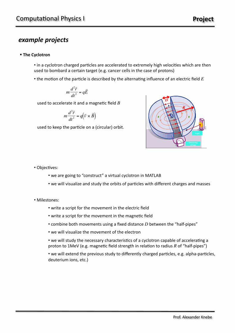
"  The Cyclotron

•  in a cyclotron charged par5cles are accelerated to extremely high veloci5es which are then used to bombard a certain target (e.g. cancer cells in the case of protons)

•  the mo5on of the par5cle is described by the alterna5ng influence of an electric field E

used to accelerate it and a magne5c field B

used to keep the par5cle on a (circular) orbit.

•  Objec5ves: •  we are going to “construct” a virtual cyclotron in MATLAB

•  we will visualize and study the orbits of par5cles with different charges and masses

•  Milestones:

•  write a script for the movement in the electric field

•  write a script for the movement in the magne5c field

•  combine both movements using a fixed distance D between the “half-‐pipes”

•  we will visualize the movement of the electron

•  we will study the necessary characteris5cs of a cyclotron capable of accelera5ng a proton to 1MeV (e.g. magne5c field strength in rela5on to radius R of “half-‐pipes”) •  we will extend the previous study to differently charged par5cles, e.g. alpha-‐par5cles, deuterium ions, etc.)

€

m d2! r dt 2

= q! E

€

m d2! r dt 2

= q ! v ×! B ( )

alterna5ng voltage

target

D

R


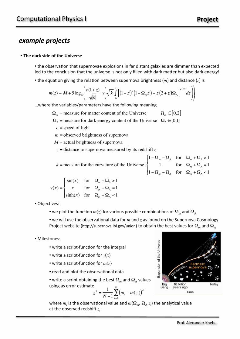
"  The dark side of the Universe

•  the observa5on that supernovae explosions in far distant galaxies are dimmer than expected led to the conclusion that the universe is not only filled with dark maaer but also dark energy!

•  the equa5on giving the rela5on between supernova brightness (m) and distance (z) is

…where the variables/parameters have the following meaning

•  Objec5ves: •  we plot the func5on m(z) for various possible combina5ons of Ωm and ΩΛ

•  we will use the observa5onal data for m and z as found on the Supernova Cosmology Project website (hap://supernova.lbl.gov/union) to obtain the best values for Ωm and ΩΛ

•  Milestones:

•  write a script-‐func5on for the integral•  write a script-‐func5on for γ(x)

•  write a script-‐func5on for m(z)

•  read and plot the observa5onal data •  write a script obtaining the best Ωm and ΩΛ values using as error es5mate where mi is the observa5onal value and m(Ωm, ΩΛ,zi) the analy5cal value at the observed redship zi


example projects

€

Ωm = measure for matter content of the Universe Ωm ∈ 0,2[ ]ΩΛ = measure for dark energy content of the Universe ΩΛ ∈[0,1]c = speed of lightm = observed brightness of supernovaM = actual brightness of supernovaz = distance to supernova measured by its redshift z

k = measure for the curvature of the Universe1−Ωm −ΩΛ for Ωm +ΩΛ >1

1 for Ωm +ΩΛ =11−Ωm −ΩΛ for Ωm +ΩΛ <1

&

' (

) (

γ(x) =

sin(x) for Ωm +ΩΛ >1x for Ωm +ΩΛ =1

sinh(x) for Ωm +ΩΛ <1

&

' (

) (

€

m(z) = M + 5log10c(1+ z)

kγ k 1+ # z ( )2 1+Ωm # z ( ) − # z 2 + # z ( )ΩΛ[ ]

−1/ 2d # z

0

z

∫(

) *

+

, -

(

) * *

+

, - -

€

χ2 =1

N −1mi −m(zi)( )2

i=1

N

∑



example projects

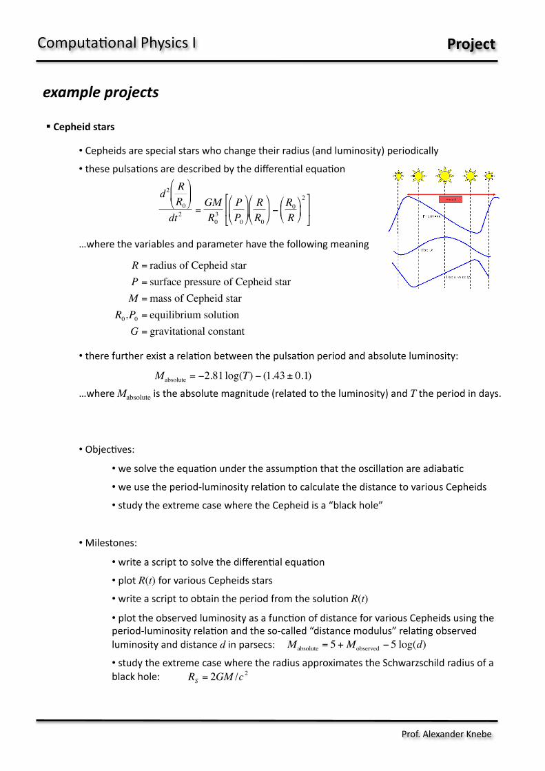
"  Cepheid stars

•  Cepheids are special stars who change their radius (and luminosity) periodically

•  these pulsa5ons are described by the differen5al equa5on

…where the variables and parameter have the following meaning

•  there further exist a rela5on between the pulsa5on period and absolute luminosity:

…where Mabsolute is the absolute magnitude (related to the luminosity) and T the period in days.

•  Objec5ves: •  we solve the equa5on under the assump5on that the oscilla5on are adiaba5c

•  we use the period-‐luminosity rela5on to calculate the distance to various Cepheids

•  study the extreme case where the Cepheid is a “black hole”

•  Milestones:

•  write a script to solve the differen5al equa5on •  plot R(t) for various Cepheids stars •  write a script to obtain the period from the solu5on R(t)

•  plot the observed luminosity as a func5on of distance for various Cepheids using the period-‐luminosity rela5on and the so-‐called “distance modulus” rela5ng observed luminosity and distance d in parsecs: •  study the extreme case where the radius approximates the Schwarzschild radius of a black hole:

€

R = radius of Cepheid starP = surface pressure of Cepheid starM = mass of Cepheid star

R0,P0 = equilibrium solutionG = gravitational constant

€

d2 RR0

"

# $

%

& '

dt 2=GMR03

PP0

"

# $

%

& ' RR0

"

# $

%

& ' −

R0R

"

# $

%

& ' 2)

* +

,

- .

€

Mabsolute = −2.81 log(T) − (1.43 ± 0.1)

€

Mabsolute = 5 + Mobserved − 5 log(d)

€

RS = 2GM /c 2



example projects

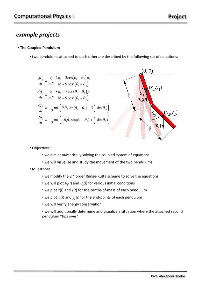
"  The Coupled Pendulum

•  two pendulums aaached to each other are described by the following set of equa5ons:

•  Objec5ves: •  we aim at numerically solving the coupled system of equa5ons

•  we will visualize and study the movement of the two pendulums

•  Milestones:

•  we modify the 2nd order Runge-‐Kuaa scheme to solve the equa5ons

•  we will plot θ1(t) and θ2(t) for various ini5al condi5ons •  we plot x(t) and y(t) for the centre-‐of-‐mass of each pendulum

•  we plot xl(t) and yl (t) for the end-‐points of each pendulum

•  we will verify energy conserva5on •  we will addi5onally determine and visualize a situa5on where the aaached second pendulum “5ps over”

€

dθ1

dt=

6ml2

2p1 − 3cos θ1 −θ2( )p2

16 − 9cos2 θ1 −θ2( )dθ2

dt=

6ml2

8p2 − 3cos θ1 −θ2( )p1

16 − 9cos2 θ1 −θ2( )dp1

dt= −

12ml2 ˙ θ 1 ˙ θ 2 sin(θ1 −θ2) + 3 g

lsin(θ1)

$

% &

'

( )

dp2

dt= −

12ml2 − ˙ θ 1 ˙ θ 2 sin(θ1 −θ2) +

gl

sin(θ2)$

% &

'

( )



example projects

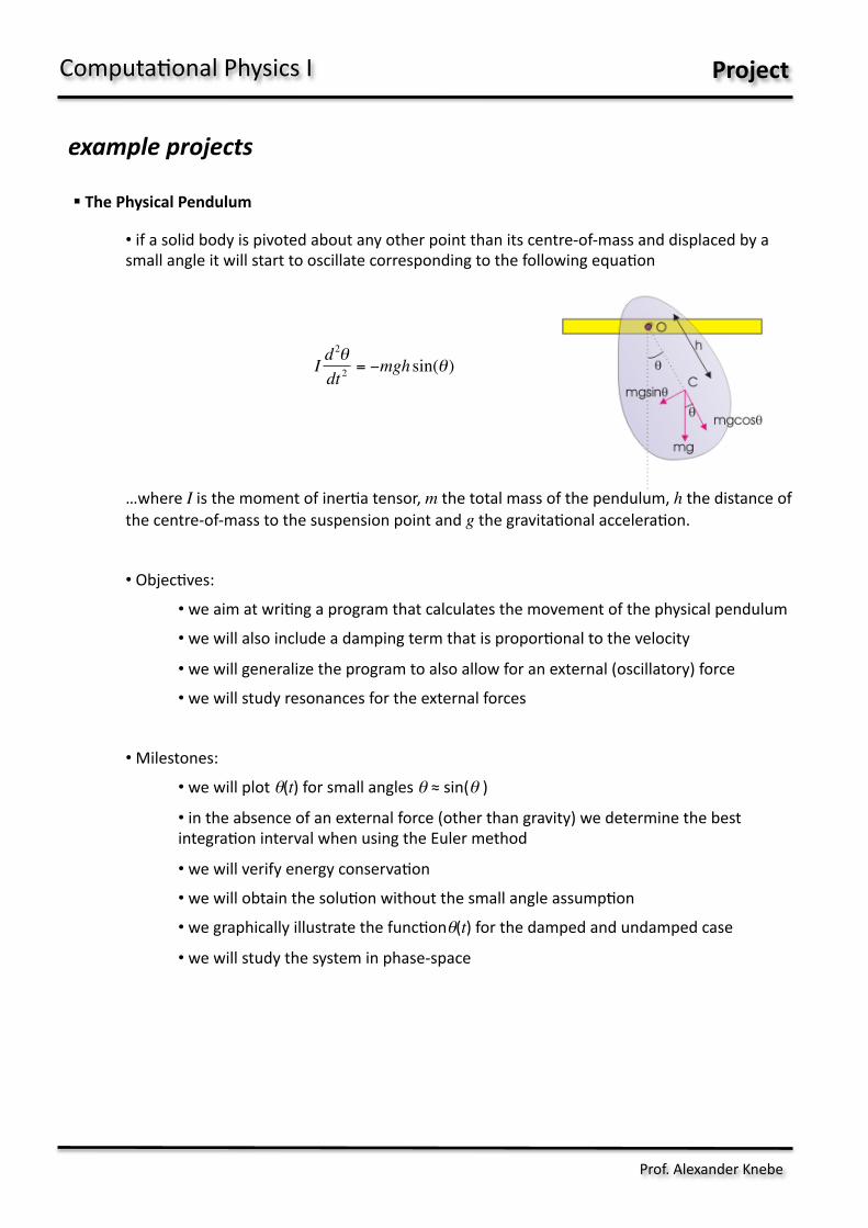
"  The Physical Pendulum

•  if a solid body is pivoted about any other point than its centre-‐of-‐mass and displaced by a small angle it will start to oscillate corresponding to the following equa5on

…where I is the moment of iner5a tensor, m the total mass of the pendulum, h the distance of the centre-‐of-‐mass to the suspension point and g the gravita5onal accelera5on.

•  Objec5ves: •  we aim at wri5ng a program that calculates the movement of the physical pendulum

•  we will also include a damping term that is propor5onal to the velocity

•  we will generalize the program to also allow for an external (oscillatory) force

•  we will study resonances for the external forces

•  Milestones:

•  we will plot θ(t) for small angles θ ≈ sin(θ )

•  in the absence of an external force (other than gravity) we determine the best integra5on interval when using the Euler method

•  we will verify energy conserva5on •  we will obtain the solu5on without the small angle assump5on

•  we graphically illustrate the func5onθ(t) for the damped and undamped case

•  we will study the system in phase-‐space

€

I d2θdt 2

= −mgh sin(θ)



more possible projects…

Earth’s Magne.c Field


Lo que nos interesa en realidad no es el vector fuerza, sino el vector aceleración (a) de la partícula en ese punto, de forma que se pueda obtener su trayectoria según la Ec. 2:

(2)

donde m es la masa de la partícula. La trayectoria la obtenemos mediante la integración numérica de la ecuación de la aceleración (Ec. 2). 2. Resultados 2.1. Primer objetivo: Observar el campo magnético terrestre. Para observar el campo magnético terrestre necesitamos conocerlo primero. Para ello, utilizaremos una función descargada de la página de Matlab que nos calcula el campo magnético terrestre (con los datos del modelo IGRF) dadas unas coordenadas espaciotemporales. Una vez tenemos el campo magnético terrestre en varios puntos, podemos representarlo. Para representar el campo y la tierra, hemos utilizado una variación del script de Matlab eliminando todo lo que no nos resultaba necesario, y así poder visualizar el campo magnético terrestre correctamente.

Figura 1.- La Tierra con sus líneas de campo magnético representadas en color rojo.

En la Figura 1 se muestra la Tierra con sus líneas de campo magnético, representadas en rojo. Las líneas de campo son una serie de puntos donde el campo magnético es constante, para una misma línea de campo. Realmente, las líneas campo son mucho más numerosas que las que se representan en la Figura 1, pero si representamos todas

Foucault Pendulum

Hohmann Orbits for Space-‐Ships

17

Analizando las imágenes de la izquierda en la Figura 4.1.2, podemos estudiar el efecto de la

variación de los valores de m,n en el patrón final. Podemos comprobar así que m determina el

número de líneas nodales en la dirección y, y n en la dirección x: si observamos la

Fig.4.1.2. Patrones obtenidos en Matlab para los modos (2,2), (1,1), (2,1) y (0,3), y su

correspondiente representación tridimensional.

Chladni Figures

your favourite system!?

Computaonal&Physics&I Project...

Documents

Transcript of Computaonal&Physics&I Project...