Computable Analysis Over the Generalized Baire Space

Computable Analysis Over the Generalized Baire Space

MSc Thesis (Afstudeerscriptie)

written by

Lorenzo Galeotti(born May 6th, 1987 in Viterbo, Italy)

under the supervision of Prof. Dr. Benedikt Lowe and Drs. Hugo Nobrega, and submitted to theBoard of Examiners in partial fulfillment of the requirements for the degree of

MSc in Logic

at the Universiteit van Amsterdam.

Date of the public defense: Members of the Thesis Committee:July 21st, 2015 Dr. Alexandru Baltag (Chair)

Dr. Benno van den BergDr. Yurii KhomskiiProf. Dr. Benedikt LoweDrs. Hugo NobregaDr. Arno PaulyDr. Benjamin Rin

Contents

1 Introduction 1

2 Basics 42.1 Orders, Fields and Topology . . . . . . . . . . . . . . . . . . . . . . . . . . . . . . . . . . . . . 42.2 Groups and Fields Completion . . . . . . . . . . . . . . . . . . . . . . . . . . . . . . . . . . . 72.3 Surreal Numbers . . . . . . . . . . . . . . . . . . . . . . . . . . . . . . . . . . . . . . . . . . . 10

2.3.1 Basic Definitions . . . . . . . . . . . . . . . . . . . . . . . . . . . . . . . . . . . . . . . 102.3.2 Operations Over No . . . . . . . . . . . . . . . . . . . . . . . . . . . . . . . . . . . . . 132.3.3 Real Numbers and Ordinals . . . . . . . . . . . . . . . . . . . . . . . . . . . . . . . . . 152.3.4 Normal Form . . . . . . . . . . . . . . . . . . . . . . . . . . . . . . . . . . . . . . . . . 16

2.4 Baire Space and Generalized Baire Space . . . . . . . . . . . . . . . . . . . . . . . . . . . . . 172.5 Computable Analysis . . . . . . . . . . . . . . . . . . . . . . . . . . . . . . . . . . . . . . . . . 19

2.5.1 Effective Topologies and Representations . . . . . . . . . . . . . . . . . . . . . . . . . 192.5.2 Subspaces, Products and Continuous Functions . . . . . . . . . . . . . . . . . . . . . . 212.5.3 The Weihrauch Hierarchy . . . . . . . . . . . . . . . . . . . . . . . . . . . . . . . . . . 22

3 Generalizing R 243.1 Completeness and Connectedness of Rκ . . . . . . . . . . . . . . . . . . . . . . . . . . . . . . 243.2 κ-Topologies . . . . . . . . . . . . . . . . . . . . . . . . . . . . . . . . . . . . . . . . . . . . . . 263.3 Analysis Over Super Dense κ-real Extensions of R . . . . . . . . . . . . . . . . . . . . . . . . 293.4 The Real Closed Field Rκ . . . . . . . . . . . . . . . . . . . . . . . . . . . . . . . . . . . . . . 323.5 Generalized Descriptive Set Theory . . . . . . . . . . . . . . . . . . . . . . . . . . . . . . . . . 42

4 Generalized Computable Analysis 524.1 Wadge Strategies . . . . . . . . . . . . . . . . . . . . . . . . . . . . . . . . . . . . . . . . . . . 524.2 Computable Analysis Over κκ . . . . . . . . . . . . . . . . . . . . . . . . . . . . . . . . . . . . 544.3 Restrictions, Products and Continuous Functions Representations . . . . . . . . . . . . . . . . 584.4 Representations for Rκ . . . . . . . . . . . . . . . . . . . . . . . . . . . . . . . . . . . . . . . . 634.5 Generalized Choice Principles . . . . . . . . . . . . . . . . . . . . . . . . . . . . . . . . . . . . 684.6 Baire Choice Functions . . . . . . . . . . . . . . . . . . . . . . . . . . . . . . . . . . . . . . . . 764.7 Representation of the IVT . . . . . . . . . . . . . . . . . . . . . . . . . . . . . . . . . . . . . . 79

5 Conclusions and Open Questions 855.1 Summary . . . . . . . . . . . . . . . . . . . . . . . . . . . . . . . . . . . . . . . . . . . . . . . 855.2 Future Work . . . . . . . . . . . . . . . . . . . . . . . . . . . . . . . . . . . . . . . . . . . . . 865.3 Open Questions . . . . . . . . . . . . . . . . . . . . . . . . . . . . . . . . . . . . . . . . . . . . 87

1

Abstract

One of the main goals of computable analysis is that of formalizing the complexity of theorems fromreal analysis. In this setting Weihrauch reductions play the role that Turing reductions do in standardcomputability theory. Via coding, we can transfer computability and topological results from the Bairespace ωω to any space of cardinality 2ℵ0 , so that e.g. functions over R can be coded as functions over theBaire space and then studied by means of Weihrauch reductions. Since many theorems from analysis can bethought to as functions between spaces of cardinality 2ℵ0 , computable analysis can then be used to studytheir complexity and to order them in a hierarchy.

Recently, the study of the descriptive set theory of the generalized Baire spaces κκ for cardinals κ > ωhas been catching the interest of set theorists. It is then natural to ask if these generalizations can be usedin the context of computable analysis.

In this thesis we start the study of generalized computable analysis, namely the generalization of com-putable analysis to generalized Baire spaces. We will introduce Rκ, a Cauchy-complete real closed field ofcardinality 2κ with κ uncountable. We will prove that Rκ shares many features with R which have a keyrole in real analysis. In particular, we will prove that a restricted version of the intermediate value theoremand of the extreme value theorem hold in Rκ.

We shall show that Rκ is a good candidate for extending computable analysis to the generalized Bairespace κκ. In particular, we generalize many of the most important representations of R to Rκ and we showthat these representations are well-behaved with respect to the interval topology over Rκ.

In the last part of the thesis, we begin the study of the Weihrauch hierarchy in this generalized context.We generalize some of the most important choice principles which in the classical case characterize theWeihrauch hierarchy. Then we prove that some of the classical Weihrauch reductions can be extended tothese generalizations. Finally we will start the study of the restricted version of the intermediate valuetheorem which holds for Rκ from a computable analysis prospective.

Chapter 1

Introduction

Computable Analysis

Computable analysis is the study of the computational properties of real analysis. We refer the reader to[28] and [6] for an introduction to classical computable analysis.

In classical computability theory one studies the properties of functions over natural numbers and thentransfers these properties to arbitrary countable spaces via coding. The same approach is taken in computableanalysis.

One of the main tools of computable analysis is the Baire space ωω, namely the space of sequence ofnatural numbers of length ω. Following the classical computability theory approach, computational andtopological properties of ωω are studied and then transferred to spaces of cardinality 2ℵ0 via coding.

R ooCoding

ωω

Of particular interest in computable analysis is the study of the computational and topological content oftheorems from classical analysis. The idea is that of formalizing the complexity of theorems by means similarto those used in computability theory to classify functions over the natural numbers. In this context, theWeihrauch theory of reducibility plays a predominant role. For an introduction to the theory of Weihrauchreductions see [5]. Weirauch reductions can be used to classify functions over the Baire space ωω. Intuitively,a function f : ωω → ωω is said to be Weihrauch reducible to g : ωω → ωω if there are two continuous functionswhich translate f into g as shown in the following commuting diagram:

ωω

f

��

Input Translation// ωω

g

��

ωω ooOutput Translation

ωω

Many theorems from classical analysis can be stated as formulas of the type:

∀x ∈ X∃y ∈ Y. ϕ(x, y),

with ϕ a quantifier-free formula. These formulas can be formalized by using multi-valued functions. Amulti-valued function T : X ⇒ Y is a function that given an element x of X returns a subset of Y . Let usconsider two classical examples, namely the Intermediate Value Theorem and the Baire Category Theorem.

The statement of the Intermediate Value Theorem is the following:For every continuous function f : [a, b] → R such that f(a) · f(b) < 0 there is a real number c ∈ [a, b] suchthat f(c) = 0. Therefore it can be stated as follows:

∀f ∈ C[a,b]∃c ∈ [a, b]. f(c) = 0,

1

where C[a,b] is the set of continuous functions f : [a, b]→ R such that f(a) · f(b) < 0. We can formalize thisformula by the following multi valued function:

IVT : C[a,b] ⇒ [a, b],

where, given a function f ∈ C[a,b], the set IVT(f) ⊂ [a, b] is such that

c ∈ IVT(f)⇒ f(c) = 0.

The Baire Category Theorem can be stated as follows:Given a countable sequence of closed nowhere dense subsets (An)n∈ω of a complete separable metric spaceX, the set X \

⋃n∈ω An is not empty.

Therefore it can be formalized by the following multi valued function:

BCT : A(X)N ⇒ X,

where A(X)N is the set of the countable sequences of closed nowhere dense subsets of X. Given a sequence(An)n∈ω, we have that:

BCT((An)n∈ω) ∈ X \⋃n∈ω

An.

The previous two examples show that even though both the Intermediate Value Theorem and the BaireCategory Theorem have a similar logical form, the multi-valued functions that represent them are quitedifferent. It seems then really impractical to compare these two multi-valued functions directly. Thisapparent difficulty can be overcome by using the Baire space.

A multi-valued function T : X ⇒ Y is usually coded within the Baire space as the set of functionst : ω → ω such that for every p ∈ ωω, we have that C(f(p)) ∈ T (C(p)) where C is the function coding Xin ωω. Given two multi-valued functions T1 : X1 ⇒ Y1 and T2 : X2 ⇒ Y2 one can therefore compare theircomplexity by studying the Weihrauch reducibility of their codings. In particular, one can study what isthe relationship, with respect to Weihrauch reducibility, of the representations of T1 and T2. For this reasonit is natural to use the Weihrauch theory of reducibility to compare theorems from analysis. The followingdiagram illustrates the situation for IVT and BCT:

C[a,b]

IVT

��

ooCoding

ωωTranslation

++kk

Translation

ivt

��

ωω

bct

��

Coding// A(X)N

BCT

��

[a, b] ooCoding

ωωTranslation

++kk

Translation

ωωCoding

// X

By using this technique it is possible to arrange many theorems from classical real analysis in a complexityhierarchy called the Weihrauch hierarchy. A study of the Weihrauch degrees of the most important theoremsfrom real analysis can be found in [5] and [2].

Generalized Baire Spaces

Recently, generalizations of the Baire space to uncountable cardinals have been of great interest for descriptiveset theorists. We refer the reader to [13] for an introduction to generalized descriptive set theory. Even thoughthe theory of generalized Baire spaces κκ with κ uncountable is not a new concept in set theory, many aspectsof this theory are still unknown. In particular it is still unclear how these generalizations can be used in thecontext of computable analysis.

In this thesis we will begin for the first time the study of generalized computable analysis, namely thegeneralization of computable analysis to generalized Baire spaces. Given a space M of cardinality 2κ, theidea is that of substituting the Baire space ωω with the generalized Baire space κκ and then of developingthe machinery necessary in order to transfer topological properties form κκ to M . In particular we will beinterested in the study of the Weihrauch hierarchy in the context of generalized Baire spaces.

Since in classical computable analysis and classical Weihrauch theory the field of real numbers has acentral role, a question arises naturally:

2

What is the right generalization of R in the context of generalized computable analysis?

R

Generalization��

ooCoding

ωω

Generalization

��

? ooCoding

κκ

One of the main results of this thesis is the definition of Rκ, a generalization of the real line which provides awell-behaved environment for generalizing real analysis and for developing generalized computable analysis.

Generalizations of the Real Line

The problem of generalizing the real line is not new in mathematics. Different approaches have been triedfor very different proposes. A good introduction to these numbers systems can be found in [12]. Among themost influential contributions to this field particularly important are the works of Sikorski [26] and Klaua [18]on the real ordinal numbers and that of Conway [9] on the surreal numbers. Sikorski’s idea was to repeat theclassical Dedekind construction of the real numbers starting from an ordinal equipped with the Hessenbergoperations (i.e., commutative operations over the ordinal numbers). Later Klaua extended Sikorski’s workproviding a complete study of this number system. Unfortunately the real ordinal numbers do not behavewell in terms of analysis. In particular one can prove that these fields do not have the density propertiesthat, as we will see, will have a central role in this context.

The surreal numbers were introduced by Conway in order to generalize both the Dedekind constructionof real numbers and the Cantor construction of ordinal numbers. In his introduction to surreal numbers,Conway proved that they form a (class) real closed field (i.e., they have the same first order properties as thereal numbers). Later, Dries and Ehrlich [18] proved that every real closed field is isomorphic to a subfield ofthe surreal numbers, showing therefore that they behave like a universal (class) model for real closed fields.It is then natural for us to use this framework in the development of Rκ.

Our Results

As we will see, doing analysis over field extensions of R is not an easy task. In particular, this is due to thefact that no proper ordered field extension of R is connected. Intuitively this means that no such extensioncan be a linear continuum in the topological sense, namely it has many holes that can be detected by theinterval topology. This is of course a problem if we want to do real analysis because many basic theorems ofreal analysis are in fact strongly related, sometimes even equivalent, to the fact that R is a connected space.To overcome this problem, instead of using standard topological tools, we will use a different mathematicalframework which, under specific conditions over the density of Rκ, will allow us to see our field extension ofR as a linear continuum. By using these tools, we will prove some basic facts from classical analysis overRκ. In particular, since the Intermediate Value Theorem and the Extreme Value Theorem are two of thepillars of real analysis on which many others concepts rely, we will place particular attention on them.

The second part of this thesis will be devoted to the study of generalized computable analysis. Inparticular we will generalize the standard machinery from computable analysis by using generalized Bairespaces. Then we will start the study of Rκ from a computable analysis point of view, showing that, becauseof its properties, Rκ fits perfectly the role of extension of R to the generalized Baire space κκ. In particularwe will show that many of the classical codings of R generalize naturally to Rκ.

In the last part of this thesis, we will use all of the generalized tools we have developed to start thestudy of the Weihrauch hierarchy over Rκ. We will show that some results from classical Weihrauch theorycan be carried over to Rκ and κκ. In particular we will generalize some of the choice principles introducedby Brattka and Gherardi in [5] and we will show that, by generalizing the classical proofs, many classicalresults hold over these generalizations. Finally we will use these generalized choice principles to start theclassification of the Rκ version the IVT.

3

Chapter 2

Basics

Before we start with the basic notions we will need to develop our theory of generalized computable analysis,we want to stipulate the following convention:

In this thesis, κ will refer to a fixed cardinal larger than ω. Moreover, since we are extending R tothe generalized Baire space κκ, we will assume κ<κ = κ. This is a standard requirement in generalizeddescriptive set theory. Moreover, since one of the essential features of ω that makes computable analysiswork is that ω<ω = ω, it is natural for us to assume1:

ASSUMPTION: κ<κ = κ.

2.1 Orders, Fields and Topology

Orders, ordered fields and topologies will be central concepts all over this thesis. In this section we will recallsome of the basic definitions and properties of ordered sets, ordered fields and topological spaces. We startwith the definition of partial order:

Definition 2.1.1 (Partial Order). Let P be a set and ≤ be a binary relation over P such that:

• ∀p ∈ P. p ≤ p (Reflexivity).

• ∀p, q ∈ P. p ≤ q ∧ q ≤ p⇒ p = q (Antisymmetry).

• ∀p, q, z ∈ P. p ≤ q ∧ q ≤ z ⇒ p ≤ z (Transitivity).

then (P,≤) is called a partial order. Moreover if

∀p, q ∈ P. p ≤ q ∨ q ≤ p ∨ p = q,

then (P,≤) is called a total (or linear) order. A totally ordered subset of a partial order is called a chain.

As usual if p, q ∈ P are such that p ≤ q and p 6= q then we will write p < q (p is strictly smaller thanq). Given two subsets A and B of a partial order (P,≤) we use the convention of writing A < B if everyelement a ∈ A is strictly smaller than every element of B.

Definition 2.1.2. Let (P,≤) be a totally ordered set and A be a subset of P . Then we have:

• P is dense iff ∀p, q ∈ P. p < q ⇒ ∃r ∈ P. p < r < q.

• A ⊆ P is dense in P iff ∀p, q ∈ P. p < q ⇒ ∃a ∈ A. p < a < q.

• A ⊆ P is cofinal in P iff ∀p ∈ P.∃a ∈ A. p ≤ a.

• A ⊆ P is coinitial in P iff ∀p ∈ P.∃a ∈ A. a ≤ p.

1From now on, whenever we use the symbol κ we assume that it satisfies this assumption without further specification.

4

We will call cofinality of P the smallest cardinal κ′ such that there is a cofinal subset of P of cardinality κ′.We will denote the cofinality of P with Cof(P ). Similarly, we will call coinitiality of P the smallest cardinalκ′ such that there is a coinitial subset of P of cardinality κ′. We denote the coinitiality of P with Coi(P ).Finally we will call weight of P , w(P ) the smallest cardinal κ′ such that there is a dense subset of P ofcardinality κ′.

Let us illustrate this notions by using a familiar example. Let R be the set of real numbers endowed withthe usual order. Then (R,≤) is a total order and Q, the set of rational numbers, is dense in R. MoreoverN, the set of natural numbers, is cofinal in R but is not coinitial, while Z, the set of integer numbers, isboth cofinal and coinitial in R. As one can imagine cofinality, coinitiality and weight are three importantproperties of an ordered set, and as we will see they will be central in most of our constructions.

Definition 2.1.3. Let (P,≤) be a totally ordered set. Then a sequence over P is an injective functionS = (xi)i∈α whose domain is an ordinal α and codomain is P . α is the length of s and will be denoted as|S|. A sequence is strictly increasing if for all γ, β < α, such that γ < β then xγ < xβ. Similarly, a sequenceis strictly decreasing if for all γ, β < α, such that γ < β we have xβ < xγ .

Definition 2.1.4. Let (P,≤) be a total order, α and β be two ordinals, s1 = (xi)i∈α and s2 = (yi)i∈β betwo sequences over P . Then we define:

• for γ < α, s1�γ = (xi)i∈γ , the restriction of s1 to γ.

• For p ∈ P , s_1 p = (xi)i∈α+1 where xα = p, the extension of s1 by p. More generally we define s_1 s2 asthe concatenation of s1 and s2. We will sometimes omit the symbol _, writing s1s2 instead of s_1 s2.

• s1 ⊆ s2 iff there is γ < β such that s1 = s2�γ, in this case we say that s1 is a prefix of s2.

• s1 / s2 iff there are γ < β such that for all i < |s1|, xi = yγ+i, namely if s1 is a subsequence of s2.

Let us illustrate the previous concepts with an example.

Example 2.1.5. Let α be an ordinal and {0, 1}<α be the set of sequences with domain in κ. We have0011010 ∈ {0, 1}<α and the sequence 1β of β ones is in {0, 1}<α if β < α. Then 0011010_1β ∈ {0, 1}<αis the sequence 0011010 followed by β ones. We have that 00 ⊂ 0011010, 1 6⊂ 0011010, 101 / 0011010 and111 6 0011010.

Now we will recall two fundamental properties of orders introduced by Hausdorff, which will becomeextremely important later in this thesis.

Definition 2.1.6. Let (P,≤) be a totally ordered set and κ′ be a cardinal. Then we have:

• P is an ακ′ -set iff every subset of P has a cofinal and coinitial subset of cardinality less than κ′.

• P is an ηκ′ -set iff given L,R ⊆ P , such that L < R and |L| + |R| < κ′ then there is x ∈ P such thatL < {x} < R.

In particular ηκ′ -sets for κ′ uncountable are interesting. Intuitively a set X is an ηκ′ -set if it is verydense, namely if in order to find an hole in the space unbounded sets of cardinality at least κ′ are necessary.

Now that we have introduced all the basic definitions about orders we can start considering orderedgroups and fields. We refer the reader to [8] for a complete introduction to field theory. We will recall somedefinitions that will be important in this thesis.

Definition 2.1.7 (Ordered Group). Let (G,+, 0) be a group and < be an order relation over G. Then(G,+, 0, <) is an ordered group iff

∀a, b, c ∈ G. a ≤ b⇒ a+ c ≤ b+ c.

We will denote the set of element of G which are strictly bigger than 0 with G+. Moreover if G is an orderedgroup we will say that G has degree κ′ iff Coi(G+) = κ′. We will denote the degree of G by Deg(G).

5

Let us illustrate these notions by two examples. The integers endowed with classical order and additionform an ordered group. Note, that Z+ has a minimum (i.e., 1), therefore Deg(Z) = 1. The rational numberswith their standard order and addition also form a group of degree ω. It is easy to see that the sequence( 1n )n∈ω is coinitial in Q+. Moreover, by the density of Q for every finite sequence of positive rational numbers

(qn)n<m there is q ∈ Q such that0 < q < {qn | n < m},

therefore (qn)n<m can not be coinitial in Q+.Given an ordered group we can define the absolute value of a ∈ G as follows:

|a| =

{a if a ≥ 0

−a otherwise.

It is easy to see that|a+ b| ≤ |a|+ |b|

for every a, b ∈ G.

Definition 2.1.8 (Ordered Field). Let (K,+, 0, 1, ·) be a field and < be an order relation over K. Then(K,+, ·, <) is an ordered field iff:

• (K,+, <) is an ordered group.

• For every a, b ∈ K bigger than 0, 0 ≤ a · b.

Using this definitions is not hard to see that many of the inequalities used in algebra hold for orderedfields. For example we have the following:

• 0 < 1.

• For all a, b, c ∈ K, a 0 implies a · c 0.

• For all a, b, c ∈ K, a 0.

• For all a, b ∈ K, a 0 implies a−1 > b−1.

The most important examples of ordered fields are the set of rational numbers Q and the set of real numbersR endowed with the standard ordering and operations. As we said in the introduction one of the main aimof this thesis is that of finding a generalization of the field of real numbers which can be used in the contextof computable analysis over the generalized Baire space κκ. It is natural then to focus on those fields whichhave the same (first order) properties of R. Fields of this kind, form a special subclass of fields:

Definition 2.1.9 (Real Closed Field). A field K is real closed if every positive a ∈ K is a square and ifevery polynomial of odd degree with coefficients in K has a root.

It is a well known fact that the theory of real closed fields in the language (+, ·, 0, 1, <) is model complete(i.e. every embedding of real closed fields is elementary). In particular it is easy to see that since the theoryof real closed fields is model complete, every real closed field K is elementary equivalent to R. In fact, letK be a real closed field. Since K has characteristic zero, Q is embedded in K. Therefore, the field of realalgebraic numbers is an elementary submodel of K (note that the real algebraic numbers are the smallest realclosed field containing Q see [19]). Now, since the field of real algebraic number is known to be elementaryequivalent to R (see [20]), all the first order properties of R transfer to K. In particular this implies that thetheory of real closed fields is complete. We refer a reader interested to the model theory of real closed fieldsto [20].

We conclude this section by recalling some basic notions from topology which will be particularly impor-tant for our constructions. We will use definitions and terminology from [22]. First recall that a topologicalspace (X, τ) is T0 if for every x, y ∈ X there is an open set U ∈ τ such that x ∈ U and y /∈ U , is secondcountable if it has a countable base and is separable if it has a countable dense subset.

6

The order on R and the topology induced by this order have a central role in this field. Let (X,≤) bean ordered set. The interval topology over X is defined as the topology generated by the base B defined asfollows:

• (a, b) ∈ B for every a, b ∈ X such that a < b.

• If b0 is the maximum in M , then (a, b0] ∈ B for every a ∈ X.

• If a0 is the minimum in M , then [a0, b) ∈ B for every b ∈ X.

The most important example of order topology is the topology on R generated by the open intervals of realnumbers.

Another topology which will have a relevant role in our constructions is the subspace topology. Given atopology (X, τ) and a subset Y of X we define the subspace topology over Y as follows:

τY = {U ∩ Y | U ∈ τ}.

Naturally we have that the base of Y is related to that of X.

Lemma 2.1.10. Let (X, τ) be a topology, B be a base of τ and Y ⊂ X. Then

BY = {B1 ∩ Y | B1 ∈ B},

is a base for the subspace topology.

Finally, let Y be a set, (X, τ) be a topological space and f : X → Y be a surjective function. Then thefinal topology induced by f is defined as follows:

O ∈ τ iff δ−1[O] is open in dom(f).

Note that since δ is surjective and continuous with respect to the final topology, then it is a quotient map. Aswe will see final topologies will have a central role both in classical and in generalized computable analysis.

2.2 Groups and Fields Completion

In this section we will recall some basic facts about group and field completions. A complete treatment ofthese subjects can be found in [8] and [10]. All the results in this section can be found in [10]. First we willpresent a general construction of cut completion over a group G.

Definition 2.2.1. Let G be a totally ordered group and L,R ⊆ G be subsets of G such that

L < R.

We will call 〈L,R〉 a cut over G.

Definition 2.2.2. Let G be a totally ordered group and C the set of all the cuts over G. Then we say thatG is C-complete iff for every 〈L,R〉 ∈ C there is x ∈ G such that L < {x} < R.

Now we will define a general procedure which given a totally ordered dense group G and its set of cutsC, constructs a group GC which contains G and is C-complete.

First we define an order relation over C as follows:

〈L1, R1〉 ≤ 〈L2, R2〉 ⇔ ∀`1 ∈ L1∃`2 ∈ L2. `1 ≤ `2.

We define an equivalence relation ∼ over C as follows:

〈L1, R1〉 ∼ 〈L2, R2〉 ⇔ 〈L1, R1〉 ≤ 〈L2, R2〉 ∧ 〈L2, R2〉 ≤ 〈L1, R1〉.

Now we define the underlying set of GC as the quotient of C under ∼, namely

GC = C/ ∼ .

7

First of all note that for all x ∈ G we can define a cut 〈Lx, Rx〉 by taking

Lx = {y ∈ G | y < x}

andRx = {y ∈ G | y > x}

Then the mapping x 7−→ [〈Lx, Rx〉] is an embedding of G in GC .It is easy to see that, if we define the order on GC as follows:

[〈L1, R1〉] ≤ [〈L2, R2〉]⇔ 〈L1, R1〉 ≤ 〈L2, R2〉,

then the embedding preserves the order.We define the addition over GC in the following way:

[〈L1, R1〉] + [〈L2, R2〉] = [〈L1, R1〉+ 〈L2, R2〉],

where 〈L1, R1〉+ 〈L2, R2〉 is defined as follows:

〈L1, R1〉+ 〈L2, R2〉 = 〈{`1 + `2 | `1 ∈ L1, `2 ∈ L2}, {r1 + r2 | r1 ∈ R1, r2 ∈ R2}〉.

It is not hard to see that the embedding x 7−→ [〈Lx, Rx〉] also preserves +. Indeed:

[〈Lx+y, Rx+y〉] = [〈Lx + Ly, Rx +Ry〉] = [〈Lx, Rx〉] + [〈Ly, Ry〉].

It is then clear that GC is a totally ordered group. Finally we claim that GC is complete. Let 〈L,R〉 be inC. Then defining

L′ =⋃

[〈Lα,Rα〉]∈L

Lα

andR′ =

⋃[〈Lα,Rα〉]∈R

Rα,

we have that L < [〈L′, R′〉] < R in GC . Therefore GC is complete.Now, if G is an ordered field we can extend this completion in such a way that GC is also an ordered

field. We only need to define the multiplication over GC . Let x, y ∈ GC with x, y > 0, x = [〈Lx, Rx〉] andy = [〈Ly, Ry〉]. Then we define:

x · y = [〈Lx, Rx〉 · 〈Ly, Ry〉],

where 〈Lx, Rx〉 · 〈Ly, Ry〉 is defined as follows:

〈Lx, Rx〉 · 〈Ly, Ry〉 = 〈{`x · `y | `x ∈ Lx, `y ∈ Ly}, {rx · ry | rx ∈ Rx, ry ∈ Ry}〉.

Moreover we define:

x · y =

(−x) · (−y) iff x, y < 0,

−((−x) · y) iff x < 0 y > 0,

−(x · (−y)) iff x > 0 y < 0,

0 iff x = 0 ∨ y = 0.

Note that, if G is a real closed field, then GC endowed with · fulfils all the properties of a real closed field,and that x 7−→ [〈Lx, Rx〉] is a field morphism between G and GC (see [10]).

Definition 2.2.3. Let K be an ordered field and C the set of cuts over K. Then K ′ is a C-completion ofK if it is C-complete and K is isomorphic to a dense subfield of K ′.

By what we have just seen we have:

Theorem 2.2.4. Let K be an ordered field and C the set of cuts over K. Then KC is a C-completion ofK.

8

L R

ε{

Figure 2.1: A Cauchy cut.

Now note that the previous construction is a generalization of the classical Dedekind construction of thereal numbers. In particular by taking G = Q and restricting C to the set of Dedekind cuts over Q (i.e.,imposing L 6= ∅ and R 6= ∅ for every 〈L,R〉 ∈ C), we have that GC = R. Now we want to show that theclassical Cauchy completion of a field is also just a particular case of the previous construction.

Definition 2.2.5 (Cauchy cuts). Let G be a totally ordered group and 〈L,R〉 be a cut over G. We will saythat 〈L,R〉 is a Cauchy cut iff it is a cut such that, L has no maximum, R has no minimum and for eachε ∈ G+ there are ` ∈ L and r ∈ R such that r < `+ ε. We will say that G is Cauchy-complete iff for eachCauchy cut 〈L,R〉, there is x ∈ G such that L < {x} < R.

Intuitively Cauchy cuts are cuts whose elements of the left and right sets get arbitrarily close to eachother (Fig.2.1).

Definition 2.2.6. Let K be an ordered field. We will say that K ′ is a Cauchy cut completion of K iff Kis a dense subset of K ′ and K ′ is C-complete with C set of Cauchy cuts over K ′.

Theorem 2.2.7. Let K be a field and C be the set of Cauchy cuts over K. Then KC is a Cauchy cutcompletion of K.

Proof. The construction of KC we have just defined works perfectly also with C restricted to the set ofCauchy cuts over K.

Classically a Cauchy completion of an ordered field is characterized in terms of sequences as follows:

Definition 2.2.8 (Cauchy sequences). Let G be a totally ordered group, and α an ordinal. Then a sequence(xi)i∈α of elements of G is Cauchy iff:

∀ε ∈ G+∃β < α∀γ, γ′ ≥ β. |xγ′ − xγ | < ε.

The sequence is convergent if there is x ∈ G such that:

∀ε ∈ G+∃β < α∀γ ≥ β. |xγ − x| < ε.

We will call x the limit of (xi)i∈α. Given a group G it is said to be Cauchy complete iff every Cauchysequence of length Deg(G) has a limit in G.

It turns out that being Cauchy cut complete and being Cauchy complete are is equivalent notions.

Proposition 2.2.9 (Dales & Woodin). Let 〈L,R〉 a Cauchy cut in an ordered group G. Then |L| =Deg(G) = |R|.

Proof. See [10, Proposition 3.3].

Then we have the following:

Theorem 2.2.10 (Dales & Woodin). The group G is Cauchy cut complete iff G is Cauchy complete.

Proof. Assume G Cauchy cut complete, and let (xi)i∈α be a Cauchy sequence in G. For each ε ∈ G+ thereis σε > 0 such that for every i, j ≥ σε, we have |xi − xj | < ε. Define

L =⋃{(−∞, xσε − ε] | ε ∈ G+}

9

andR =

⋃{([xσε + ε,+∞) | ε ∈ G+}.

Then for every ε ∈ G+ take 0 < ε′ < ε, then take ` ∈ L, r ∈ R such that ` = xσε′ − ε′ and r = xε′ + ε′,

then `+ ε > r. Hence 〈L,R〉 is Cauchy and there is x ∈ G such that L < {x} < R as desired. Now assumethat every Cauchy sequence of length Deg(G) has a limit. Let 〈L,R〉 be a Cauchy cut in G, then by theprevious proposition it |L| = Deg(G). Then there is a strictly increasing sequence cofinal in L of cardinalityDeg(G) and it is trivially Cauchy, hence it converges to an element of x ∈ G. Then we have L < {x} < Ras desired.

Given the previous theorem, we will use the two definitions of Cauchy completion interchangeably.

2.3 Surreal Numbers

The surreal numbers were introduced by Conway [9] in order to generalize both the Dedekind construction ofreal numbers and the Cantor construction of ordinal numbers. He realized that both Dedekind and Cantorwere using a common pattern to define numbers.

As we will see even though their definition is simple, the surreal numbers form a very powerful tool forstudying different number systems.

Conway’s idea was that of generalize these two definition in order to generate both ordinals and realnumbers on the same time.

2.3.1 Basic Definitions

The following definition of surreal numbers is due to Conway and it has been deeply studied by Gonshor in[14].

Definition 2.3.1 (Surreal Numbers). A surreal number is a function from an ordinal α ∈ On to {+,−},i.e., a sequence of pluses and minuses of ordinal length. We will denote the class of surreal numbers by No.The length of a surreal number x ∈ No is the smallest ordinal |x| ∈ On for which x is not defined.

We can define a total order over No as follows:

Definition 2.3.2. Let x, y ∈ No be two surreal numbers. Then we define the following order:

x < y iff x(α) < y(α) where α is the smallest ordinal s.t. x(α) 6= y(α),

here we are using the order − < 0 < + where x(α) = 0 if x is not defined at α.

Given the previous definition it easy to see that No has a natural binary tree structure (see Fig.2.2).Note that each level of the tree corresponds to a set of surreal numbers with the same length. In particular

we can define:

Definition 2.3.3. Let No be the class of surreal numbers and α ∈ On be an ordinal. We define the followingsets:

Noα = {+,−}α i.e. the set of sequences of length exactly α,

No≤α =⋃β≤α

Noβ i.e. the set of sequences of length less or equal to α,

No<α =⋃β<α

No≤β i.e. the set of sequences of length less than α.

Note that from this definition it is not hard to see that No≤α = No<α ∪Noα and Noα = No≤α \No<α.Moreover these sets determine proper initial trees of the surreal number tree, as shown in Fig.2.3. Someof these subtrees will be of particular importance for our constructions. In particular as we will see, thefollowing theorem will be central for the constructions of Chapter 3:

10

〈〉

−

−−

......

−+

......

+

+−

......

++

......

Figure 2.2: The surreal tree.

Figure 2.3: The subtrees of No.

Theorem 2.3.4 (Alling). Let κ′ be a regular cardinal. Then No<κ′ is a real closed field.

Proof. See [1, Theorem 6.22].

An extended study of these trees can be found in [11] and [1].The following theorem will have a central role in the definition of operations over surreal numbers.

Theorem 2.3.5 (Gonshor, Simplicity Theorem). Let L and R be two sets of surreal numbers such thatL < R. Then there is a unique surreal z, denoted by [L|R], of minimal length such that L < {z} < R. Wewill call [L|R] a representation of z.


Given two finite family of sets of surreal numbers S0 . . . Sn and S′0 . . . S′m, we will use the following

notation:[S0, . . . , Sn|S′0, . . . , S′m] = [

⋃i≤n

Si|⋃i≤m

S′i].

Moreover, given two finite sequence of surreal numbers x0, . . . , xn and x′0, . . . , x′m we define:

[x0, . . . , xn|x′0, . . . , x′m] = [{x0, . . . , xn}|{x′0, . . . , x′m}].

11

Each surreal number has many different representations, the following theorem gives us a canonicalrepresentation.

Theorem 2.3.6 (Gonshor). Let x ∈ No be a surreal number, L and R be two subsets of No defined asfollows:

L = {y | x < y ∧ y ⊂ x},R = {y | x > y ∧ y ⊂ x}.

Then [L|R] = x.


We will call the representation given by Theorem 2.3.6 the canonical representation of x. Note that thecanonical representation just says that the elements of L are the proper initial segments y of x such thatx(|y|) = + and the elements of R are the proper initial segments y of x such that x(|y|) = −. For examplethe canonical representation of + − + is [(), (+−)|(+)], which means that + − + is the shortest numberbetween +− and +. As we will see, representations have an important role in developing surreal numberstheory. For this reason we will introduce some theorems which allow to manipulate and characterize theserepresentations.

Theorem 2.3.7 (Gonshor). Let L and R be two sets of surreal numbers such that L < R. Then |[L|R]| issmaller or equal to the least ordinal α such that:

∀x ∈ L ∪R. |x| < α.

Proof. Note that this follows trivially from the fact that [L|R] is defined to be de shortest surreal numberstrictly between L and R, then if it is of length bigger than α. Hence [L|R]�α would be shorter than [L|R]and still in between L and R.

Theorem 2.3.8 (Gonshor). Let x, y ∈ No be two surreal numbers and [Lx|Rx], [Ly|Ry] be respectively arepresentation of x and y. Then x ≤ y iff {x} < Ry and Lx < {y}.

Proof. We have Lx < {x} < Rx and Ly < {y} < Ry. Assume x ≤ y then trivially {x} ≤ {y} < Ry andLx < {x} ≤ {y}. Assume {x} < Ry and Lx < {y} and y < x. We have Lx < {y} < {x} < Rx hence x is aninitial segment of y. Moreover Ly < {y} < {x} < Ry then y is an initial segment of x. Hence x = y whichcontradicts our assumption.

Finally we present three theorems from [14] which are very useful to find out when two different repre-sentation represent the same surreal number.

Definition 2.3.9 (Cofinality). [L|R] is cofinal in [L′|R′] iff:

∀x′ ∈ R′∃x ∈ R. x ≤ x′ ∧ ∀y′ ∈ L′∃y ∈ L. y ≥ y′.

Moreover, given two representations [L|R] and [L′|R′] they are mutually cofinal iff [L|R] is cofinal in [L′|R′]and [L′|R′] is cofinal in [L|R].

Note that this definition is totally consistent with the standard definition of cofinality (see Definition2.1.2).

Theorem 2.3.10. Suppose x = [L|R], L′ < x < R′ and [L′|R′] cofinal in [L|R] then x = [L′|R′].

Theorem 2.3.11. Suppose [L|R] and [L′|R′] are mutually cofinal then [L|R] = [L′|R′].

12

2.3.2 Operations Over No

In this section we will define addition and multiplication over surreal numbers. First of all let us introducesome notation which will simplify the definition of the operations over surreal numbers. If S and S′ are asets of surreal numbers, x is a surreal number and Op a binary operation over the surreal numbers, then wedefine

SOpx = {sOpx|s ∈ S}, xOpS = {xOp s|s ∈ S}

andSOpS′ = {xOp y|x ∈ S ∧ y ∈ S′}.

We begin the study of the surreal operations by defining the addition and its inverse.

Definition 2.3.12 (Surreal Sum and Inverse). Let x and y be two surreal numbers and [Lx|Rx], [Ly|Ry] betheir canonical representations. Then we define the sum x+s y as follows:

x+s y = [Lx +s y, x+s Ly|Rx +s y, x+s Ry].

Moreover we define the inverse of x as the surreal number obtained by reverting all the signs. It is easy tosee that that [−Rx| − Lx] where

−Rx = {−xR | xR ∈ Rx}

and−Lx = {−xL | xL ∈ Lx},

is a canonical representation of −x.

The previous definition was given by induction over the maximal length of the addends. Note that wedefined +s and −s only for canonical representations. The following theorem tells us that the choice of therepresentations we used does not matters.

Theorem 2.3.13. Let [Lx|Rx] and [Ly|Ry] be two representations respectively of x and y. Then

x+s y = [Lx +s y, x+s Ly|Rx +s y, x+s Ry].


The intuition behind the definition of +s is that x +s y can be thought to be the smallest number suchthat the following inequalities hold:

Lx + y < x+ y < Rx + y,

x+ Ly < x+ y < x+Ry.

Then the definition of x +s y is exactly reflecting this intuition, in fact x +s y is defined to be the shortestsurreal number for which the previous inequalities hold. Let us consider some examples of sum.

Example 2.3.14. Consider the sequence + and its inverse −. Let 〈〉 be the empty sequence2. Then we have

(+) = [〈〉|∅] and (−) = [∅|〈〉],

where 〈〉 is the empty sequence. Then (+) +s (−) = [∅|∅] = 〈〉. Therefore it is natural to define 0 = 〈〉. Nowdenote (+) as 1. Finally we have

1 + 1 = (+) +s (+) = {1 +s 0, 0 +s 1|}.

We will denote this number by 2. It is not hard to convince yourself that we could interpret all the naturalnumbers in this way.

2Note that for the theory of surreal numbers 〈〉 = [∅ | ∅] 6= ∅.

13

Definition 2.3.15 (Surreal Product). Let x and y be two surreal numbers and [Lx|Rx], [Ly|Ry] be theircanonical representations. Then we define the product x ·s y as follows:

x ·s y = [Lx ·s y +s x ·s Ly − Lx ·s Ly, Rx ·s y +s x ·s Ry −Rx ·s Ry|Lx ·s y +s x ·s Ry − Lx·sRy, Rx ·s y +s x ·s Ly −Rx ·s Ly].

Also in this case the definition is by induction over the maximal length of the factors, and as beforethe definition is uniform (the interested reader is referred to [14] Theorem 3.5). Let us illustrate how thisdefinition works with an example.

Example 2.3.16. We have already defined 0 = 〈〉, 1 = + and 2 = ++. Let us consider the multiplication2 ·s 1. First note that trivially:

0 ·s 1 = 0 ·s 1 = [∅|∅] = 0

and0 ·s 2 = 0 ·s 2 = [∅|∅] = 0.

Moreover we have1 ·s 1 = [0 ·s 1 +s 1 ·s 0− 0 ·s 0|∅].

Therefore1 ·s 2 = [0 ·s 2 +s 1 ·s 1− 0 ·s 1|∅].

In conclusion 1 ·s 2 = [1|∅] = 2.

The last operation we introduce is the inverse of the product. While the previous definitions are quiteintuitive the definition for the inverse of ·s is more complicated. First of all one should convince himself thatthe naive definition, namely

1

y= [0,

1

Ly| 1

Ry]

does not work. In particular this definition is such that 1y ·s y 6= 1 for some y ∈ No. To see this it is enough

to compute some left element of 13 ·s 3 and check that it is bigger than 1. In particular we would have

13 = [0, 1, 12 |∅] and 3 = [0, 1, 2|∅]. But then 3 +s

13 −s 1 would be a left element of 1

3 ·s 3, and by using thedefinition of +s and −s we would have 3 +s

13 −s 1 > 1.

The main idea behind the definition of inverse of ·s is that of setting the values in 1y in such a way that

the left elements of 1y ·s y are smaller than 1. We define the inverse of ·s by induction over the length of y as

follows:

Definition 2.3.17 (Product Inverse). Let y ∈ No be a positive surreal number and let {Ly|Ry} be a rep-resentation of y such that Ly, Ry > {0}3. By induction over the length of y assume that the inverse hasalready been defined for Ly and Ry. We define the following sequences:

〈〉 = 0,

〈y0, . . . yn〉 = x for every y0, . . . , yn ∈ Lx ∪Rx \ {0},

where x is the solution of the equation (y −s yn) ·s 〈y0, . . . yn−1〉 + yn ·s x = 1. Note that a solution for thisequation exists by inductive hypothesis. Now we define:

1

y= [L 1

y|R 1

y],

where:L 1y

= {〈y0, . . . , yn〉 | n ∈ N the number of 0 ≤ i ≤ n such that yi ∈ Ly is even}

andR 1y

= {〈y0, . . . , yn〉 | n ∈ N the number of 0 ≤ i ≤ n such that yi ∈ Ly is odd}.

3Note that by cofinality argument such a representation always exist

14

As for the previous definitions also the definition of product inverse is uniform.A class field is a proper class C whose members satisfy the axioms of the theory of real closed fields4

(i.e., every axiom of the theory of real closed fields instantiated with members of C can be proved). Giventhis definition, we can now mention an important result:

Theorem 2.3.18. The surreal numbers No endowed with +s and ·s form a class field.


Since in this thesis we will mostly be dealing with surreal operations, when no confusion arise we willdrop the s from ·s and +s.

2.3.3 Real Numbers and Ordinals

In this section we will show how to interpret real numbers and ordinal numbers within the class field ofsurreal numbers.

Before we show how real numbers are represented we consider the easier case of integers. We have alreadygiven some basic example showing how to represent 0, 1 and 2. Our intuition lead us to think that naturalnumbers are just finite sequences of pluses. Formally we have the following theorem:

Theorem 2.3.19 (Gonshor). For all n ∈ N, (+)n is the positive integer n and (−)n is its inverse.

The dyadic rational numbers are those rational numbers of the form n2m with n ∈ Z and m ∈ N. The

surreal numbers of finite length can be identified with the ring of dyadic rational numbers as shown by thefollowing theorem:

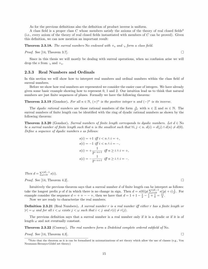
Theorem 2.3.20 (Gonshor). Surreal numbers of finite length corresponds to dyadic numbers. Let d ∈ Nobe a surreal number of finite length such that n is the smallest such that ∀i, j < n. d(i) = d(j)∧ d(n) 6= d(0).Define a sequence of dyadic numbers s as follows:

s(i) = +1 iff i < n ∧ i = +,

s(i) = −1 iff i < n ∧ i = −,

s(i) = +1

2i−n+1iff n ≥ i ∧ i = +,

s(i) = − 1

2i−n+1iff n ≥ i ∧ i = −.

Then d =∑|d|−1i=0 s(i).


Intuitively the previous theorem says that a surreal number d of finite length can be interpret as follows:

take the longest prefix p of d in which there is no change in sign. Then d = s(0)|p|∑|d|−1i=0 s(|p| + i) 1

2i . Forexample consider the sequence d = + +−−+, then we have that d = 1 + 1− 1

2 −14 + 1

8 = 118 .

Now we are ready to characterize the real numbers.

Definition 2.3.21 (Real Numbers). A surreal number r is a real number iff either r has a finite length or|r| = ω and for all i < ω exists j < ω such that i < j and r(i) 6= r(j).

The previous definition says that a surreal number is a real number only if it is a dyadic or if it is oflength ω and not eventually constant.

Theorem 2.3.22 (Conway). The real numbers form a Dedekind complete ordered subfield of No.


4Note that the theorem as it is can be formalized in axiomatizations of set theory which allow the use of classes (e.g., VonNeumann-Beranys-Godel set theory)

15

0

−1

−2

...

−ω

...

...

...

− 12

......

+1

12

......

+2

......

...+ω

...

Figure 2.4: The surreal tree.

Finally will identify every ordinal α with the constant sequence of pluses of length α. We will denotesuch a sequence by (+)α.

Note that this fits completely with the definition of positive integers we have just given. Moreover theorder is trivially preserved, namely α < β implies (+)α < (+)β . Note that α + 1 = [{β|β ≤ α}|∅] and if αis limit then α = [{β|β < α}|∅]. Then from the order theoretic point of view we can identify ordinals andsequences of pluses.

Now if we look at the operations, the situation seems different. First of all we know that surreal operationsare commutative while ordinal operations are not, for example ω +s 1 = 1 +s ω while ω + 1 6= ω = 1 + ω.In his introduction to surreal numbers Gonshor proved that the surreal operations over ordinal numberscorrespond to the Hessenberg (natural) operations.

2.3.4 Normal Form

In this section we will introduce a normal form for surreal numbers which is a generalization of Cantor’snormal form for ordinal numbers.

Definition 2.3.23 (Archimedean Equivalence Relation). Given two positive surreal numbers x and y wedefine the following equivalence relation:

x ∼a y iff ∃n ∈ Z . n ·s y ≥ x ∧ n ·s x ≥ y.

The equivalence classes induced by this relation are called orders of magnitude.

One interesting fact of the orders of magnitudes is that they have canonical representatives.

Theorem 2.3.24 (Gonshor). Let x be a positive surreal number. Then there is a unique y of minimal lengthsuch that x ∼a y.

These canonical elements can be parametrized using surreal numbers and the ω-map. Intuitively, theω-map is defined by letting ω0 be the shortest canonical element, namely 1, ω1 and ω−1 be respectively ωand 1

ω and so on. Formally we have:

16

Definition 2.3.25 (ω-map). Let x be a surreal number. We define:

ωx = [0, r ·s ωLx |s ·s ωRx ],

where s and r are positive real numbers,

ωLx = {ωxL | xL ∈ Lx}

andωRx = {ωxR | xR ∈ Rx}.

The fact that the ω-map is represented as an exponentiation is because it behaves as one would expectfrom the exponentiation operator.

Theorem 2.3.26 (Gonshor). Let x,y be two surreal numbers. We have:

• ωx ·s ωy = ωx+sy.

• If x is an ordinal then ωx is the same as the usual ordinal ωx.

• ωx ·s ω−x = 1.

In order to define the normal form of surreal numbers we need transfinite sums. Let α be an ordinal,(xγ)β∈α be a strictly decreasing sequence of α surreal numbers and (rβ)β∈α be a sequence of α non-zero realnumbers. Then we define the sum

∑β<α ω

xβ ·s rβ as follows:∑β<γ+1

ωxβ ·s rβ =∑β∈γ

ωxβ ·s rβ +s ωxγ ·s rγ if α = γ + 1,

∑β<α

ωxβ ·s rβ = [L|R] if α limit,

where L and R are defined as follows:

L = {∑γ≤β

ωxγ ·s sγ : [β < α] ∧ [∀γ < β. sγ = rγ ]∧

[sβ = rb − t with t any positive real number ]},

R = {∑γ≤β

ωxγ ·s sγ : [β < α] ∧ [∀γ < β. sγ = rγ ]∧

[sβ = rb + t with t any positive real number ]}.

Theorem 2.3.27 (Conway, Normal Form Theorem). Every surreal number can be expressed uniquely in theform

∑β∈α ω

xβ ·s rβ.


Note that the Cantor normal form is a special case of surreal numbers normal form.

2.4 Baire Space and Generalized Baire Space

In this section we will briefly recall some notion from basic descriptive set theory and generalized descriptiveset theory. All the results in the first part of this section can be found in the first chapter of any introductorybook of descriptive set theory such as [17].

Definition 2.4.1 (Baire Space). Let ωω be the set of sequences of natural numbers of length ω. For everyfinite sequence of natural numbers w ∈ ω<ω we define the following set:

[w] = {p ∈ ωω | w ⊂ p},

namely [w] is the set of infinite sequences that start with w. The set

B = {[w] | w ∈ ω<ω}

is a base. We will call the set ωω equipped with the topology induced by B Baire space.

17

Note that ωω is by definition second countable.

Lemma 2.4.2 (Folklore). Baire space is Hausdorff.

Proof. Let p, p′ ∈ ωω such that p 6= p′ and n be the smallest natural numbers such that p(n) 6= p′(n). Now[p�n] and [p′�n] are open sets. By the fact that p(n) 6= p′(n) we have that [p�n] ∩ [p′�n] = ∅. Moreover,p ∈ [p�n] and p′ ∈ [p′�n] as desired.

Baire space is easily proved to be totally disconnected.

Lemma 2.4.3 (Folklore). Baire space is totally disconnected.

Proof. We need to prove that for every w ∈ ω<ω, the set [w] is closed. Let W be defined as follows:

W = {w′ ∈ ω<ω | ∃n ∈ ω. w(n) 6= w′(n)}.

Then ωω \ [w] =⋃W . Hence ωω \ [w] is open and [w] is closed as desired.

Baire space is completely metrizable with the following metric5:

d(p, p′) =

{0 if p = p′,1

n+1 if n is the least such that p(n) 6= p′(n).

One important property of Baire space is that it is homeomorphic to the product topology∏α∈ω ω where

ω is endowed with the discrete topology.Now we will recall some basic definitions and properties of generalized Baire spaces. In particular we will

generalize the notions we have just seen to the cardinal κ we have fixed at the beginning of this chapter. Allthe notions that we will present in the rest of this section can be found in [13].

Definition 2.4.4 (Generalized Baire Space). Let κκ be the set of sequences of ordinals in κ of length κ. Forevery sequence w ∈ κ<κ of elements of κ of length less than κ, we define the following set:

[w] = {p ∈ κκ | w ⊂ p}.

Then the setB = {[w] | w ∈ κ<κ}

is a base. We will call the set κκ equipped with the topology induced by B generalized Baire space.

Note that the assumption κ<κ = κ, is necessary in order for generalized Baire space to have a base ofcardinality κ and then a dense subset of cardinality κ. As we will see this will be crucial for generalizecomputable analysis. By using the same proofs of the classical case it is not hard to see that generalizedBaire space κκ is Hausdorff and totally disconnected.

We want to end this section by mentioning to important differences between the Baire space ωω and itsuncountable generalizations.

Theorem 2.4.5. Generalized Baire space is not metrizable.

Proof. First of all recall from topology that if a space X is metrizable, then for every x ∈ X, there is acountable set Nx of open sets such that for every open set U containing x there is V ∈ N such that V ⊂ U .Assume that κκ is metrizable. Let p be an element of κκ. For every element of U ∈ Np take a basic openset [wU ] which contains x and such that [wU ] ⊂ O. Since there are only countably many of these open setsand κ is a regular cardinal bigger than ω, there is w ∈ κκ such that for every U ∈ Np, we have wU ⊂ w. Butthen x ∈ [w] and for every U ∈ Np we have U 6⊆ [w]. This contradicts our hypothesis, therefore κκ is notmeasurable.

Hence there is no notion of a metric which induces κκ. In particular this means that all the notions thatdepend on the metrizability of κκ (e.g. the Borel hierarchy) have to be either reformulated in a non-metricway or cannot be generalized to κκ.

Finally, generalized Baire space is not homeomorphic to the product topology∏α∈κ κ, where κ is endowed

with the discrete topology (see [13]).

5Note that, even though this is not the standard definition of the metric over ωω , it is completely equivalent to the classicalone from the topological point of view. As we will see in Chapter 3 this definition will generalize in a straightforward way toκκ by using Rκ.

18

2.5 Computable Analysis

In this section we will present some basic notion from classical computable analysis and we will set up someconventions that we will use all over this thesis. A complete introduction to computable analysis can befound in [28] and a topological introduction to the more general theory of represented spaces can be foundin [23]. Where it is possible, we will use the same notation as in [28].

2.5.1 Effective Topologies and Representations

The intuition behind computable analysis is that of generalizing computability theory to uncountable sets.In order to do this, the idea is that of study computational and topological properties of the Baire space ωω

(or the Cantor space 2ω) and then, transfer these results to any uncountable set by means of coding. Thesecodings have a central role in computable analysis, therefore we recall their definition.

Definition 2.5.1 (Representation). Let M be a countable set. Then a notation over M is a surjectivepartial function from the set of finite sequences of natural numbers ω<ω to M . If M has cardinality 2ℵ0 thena surjective partial function with domain the Baire space ωω and codomain M is called a representation ofM . If δ is a representation over M , we will call (M, δ) a represented space.

Definition 2.5.2 (Reductions). Let δ :⊆ ωω →M and δ′ :⊆ ωω →M be two representations of M . Then wewill say that δ continuously reduces to δ′, in symbols δ ≤t δ

′ iff there is a continuous function h :⊆ ωω → ωω

such that for every x ∈ dom(f), δ(x) = δ′(h(x)).If δ ≤t δ

′ and δ′ ≤t δ we will say that δ and δ′ are continuously equivalent and we will write δ ≡t δ′.

Continuous reductions are a very useful tool, and as we will see they can be used to see how representationsbehave with respect to the topological properties of the space they represent.

Note that usually in computable analysis to any continuous notion correspond a computable notion, forexample we could consider computable reductions instead of continuous reductions. The reason why we willonly present the topological aspects of computable analysis is that it is still not clear how to define a notionof computability over κκ.

Effective topological spaces form a particularly well-behaved subclass of spaces. They induce naturallya standard representation which turns out to be a quotient map with respect to the topology of the spacethey represent.

Definition 2.5.3 (Effective Topological Space and Standard Representation). Let M be a set, σ be acountable family of subsets of M such that

x = y iff {A ∈ σ | x ∈ A} = {A ∈ σ | y ∈ A}

and ν :⊆ ω<ω → σ be a naming on σ. Then S = (M,σ, ν) is an effective topological space. We will call τsthe topology generated by taking σ as a subbase and δS :⊆ ωω →M the standard representation of S definedas follows:

δS(p) = x iff {A ∈ σ | x ∈ A} = {ν(w) ∈ ι(w) / p} ∀p ∈ ωω.

Intuitively, given an effective topological space, we can think at σ as a list of properties that can distinguishelements of M and at ν as the way we can access them. From this point of view, p ∈ ωω is a code for x ∈Maccording to the standard representation if and only if p codes the list of all the properties which characterizex.

As we have already said, effective topological spaces are a particularly well-behaved subclass of representedspaces. This is due to the fact that in this specific case the topological space τS and the final topologyinduced by δS are the same. This implies that some important properties of τS transfer to Baire space andvice versa. The following lemma shows how strong is the connection between an effective topological spaceand its induced topology.

Lemma 2.5.4. Let S = (M,σ, ν) be an effective topological space, δS its standard representation and τS theinduced topology. We have:

• τS is the final topology induced by δS.

19

• δS is continuous and open w.r.t τS.

Proof. See [28, Lemma 3.2.5].

This lemma is important to establish a connection between Baire space and the topology τS . Let usillustrate how effective topological spaces work with an example.

Example 2.5.5. Let us consider the set of real number R. We already know that, in order to do analysisover R we will want to use the interval topology τR over R. Then it is natural look for a representationwhich induces this topology. We can use the well known fact that the set of open intervals with endpointsin Q is a base for τR and the fact that Q is countable to define an effective topological space whose inducedtopology is τR. Let νQ :⊆ ω<ω → Q be any notation over Q (it is not hard to explicitly define one). Moreoverlet p·, ·q : ω<ω × ω<ω → ω<ω be any pairing function. Then we can define a notation for the set of openintervals with rational endpoints Cb as follows:

I(pi, jq) = B(νQ(i), νQ(j)),

where B(q, q′) is the open ball with center q and radius q′. Define S = (R,Cb, I). Now, since Cb is a basefor the interval topology over R, then τS is the interval topology over R. Moreover, for what we have justshown, δS is continuous and open with respect to this topology.

Lemma 2.5.6. Let M be a set, δ0 :⊆ ωω → M and δ1 :⊆ ωω → M be two representations. Moreover, letτ0 and τ1 be respectively the final topology induced by δ0 and δ1. Then δ0 ≤t δ1 implies τ1 ⊆ τ0. Moreover,given δ′0 :⊆ ωω →M and δ′1 :⊆ ωω →M be other two representations of M , such that δ′0 ≤t δ0 and δ′1 ≤t δ1.Then every (δ0, δ1)-continuous function is (δ0, δ1)-continuous.

Proof. Let f :⊆ ωω → ωω be a continuous reduction of δ0 to δ1 and O ∈ τ1. By definition δ−11 (O) isopen in dom(δ1). Moreover, since f is continuous, f−1δ−11 (O) is open in dom(f) ∩ f−1(dom(δ1)). Thenf−1δ−11 (O) is open in dom(f) ∩ f−1(dom(δ1)) ∩ dom(δ0). Now, since f is a reduction of δ0 to δ1, we havedom(f) ∩ f−1(dom(δ1)) ∩ dom(δ0) = dom(δ0) and δ−10 (O). Hence O ∈ τ0 as desired.

Now let f be a (δ′0, δ′1)-continuous function. Consider a continuous reduction h0 of δ0 to δ′0 and a

continuous reduction h1 of δ1 to δ′1. Let F be a continuous realizer of f . Then h1 ◦ F ◦ h0 is a (δ0, δ1)-continuous realizer of f .

Since continuous reductions preserve many topological properties we are interested in, it is natural to usethem to characterize a well-behaved class of representations.

Definition 2.5.7 (Admissible Representation). Let (M, τ) be a topological space. Then a representationδ :⊆ ωω → M is κ-admissible w.r.t. τ iff δ is continuous and every continuous function ϕ :⊆ ωω → M iscontinuously reducible to δ.

Note that, as shown in [24], a representation δ of a topological space (M, τ) is admissible iff it is contin-uously equivalent to a standard representation of an effective topological space S = (M,σ, ν) with τS = τ .

In classical computability theory representations are used to transfer computability form the naturalnumbers to any countable space. The same approach is taken in computable analysis, where representationsallow to transfer notions of continuity and computability from Baire space to any space of cardinality atmost 2ℵ0 . Realizers have a central role in this construction.

Definition 2.5.8. Let F :⊆ M1 → M0 be a function over two represented spaces (M1, δ1) and (M0, δ0).Then f :⊆ ωω → ωω is a realization of F iff for every x ∈ dom(δ1), F (δ1(x)) = δ0(f(x)). If f is continuouswe will say that F has a continuous realizer w.r.t. δ1 and δ0 or for short that F is (δ1, δ0)-continuous.

Obviously it is important to define representations that induce notions of continuity and computabilitywhich are suitable for our purpose. For example, since we want to do computable analysis it makes littlesense to have a representation that does not even make addition and product continuously representable.Therefore the following theorem is of main interest for computable analysis.

20

Theorem 2.5.9 (Main Theorem of Computable analysis). For i = 0, . . . , n let δi :⊆ ωω → Mi be anadmissible representation w.r.t. the topology τi. Then for any function f :⊆M1 × . . .×Mn →M0 we have:

f is continuous ⇔ f is (δ1, . . . , δn, δ0)-continuous.

Proof. See [28, Lemma 3.2.11].

In particular the main theorem of computable analysis tells us that admissible representations respectcontinuous functions over the topological spaces they induce.

Example 2.5.10. Let us continue our example on R. Let S = (R,Cb, I) be the effective topological spacedefined in the Example 2.5.5. We know that τS is the interval topology over R. now, since is a well-knownfact that + and × are continuous over the interval topology, the main theorem of computable analysis tellsus that + and × are continuously represented over Baire space.

The main theorem of computable analysis is important in computable analysis and in all those cases inwhich we already have a standard topology over the space we want to work with. In these cases, indeed,effective topological spaces and admissible representations give us a strict correspondence between continuousfunctions between represented spaces endowed with their intended topologies and the continuous functionsover Baire space. This fact will turn out to be also important for representing the set of continuous functionsbetween representable spaces.

Note that, in some cases a completely different approach is possible. In particular if we do not have apreferred candidate for the topology we want to use over the represented space we are working with, then wecan just fix any representation and work with the final topology induced by this representation. In this casewe would still have the main theorem of computable analysis w.r.t. the final topology and then a naturalway to represent the space of continuous functions on our space.

2.5.2 Subspaces, Products and Continuous Functions

In this section we will briefly recall some constructions over representations.First of all we consider subspaces of represented spaces. Note that, since restriction of surjective functions

are still surjective, for every represented spaces (M, δM ) and subset M0 of M the restriction δM �M0 of δM toM0 is still a representation of M0. Moreover, it turns out that the restriction of admissible representationsis still admissible.

The second construction that we take into consideration is product. Before we can give the definitionof product of representations we need to define some tupling functions. Fix a bijection p·, ·q : ω × ω → ω.Then we define:

Definition 2.5.11 (Tupling Functions). Let a1, a2 . . . , ai with i < ω be a sequence of element of ω. Wedefine a wrapping function ι as follows:

ι(a1, a2, . . . , ai) = 110a10a20 . . . 0ai011.

Moreover given x1, x2, . . . in ω<ω and p1, p2 . . . , in ωω, we define:

px1, p1q = pp1, x1q = ι(x1)p1 ∈ ωω,px1, . . . , xiq = ι(x1) . . . ι(xi) with i < ω,

px1, x2 . . .q = ι(x1)ι(x2) . . . ,

pp1, . . . , piq = p1(0) . . . pi(0)p1(1) . . . pi(1) . . . with i < ω,

pp1, p2 . . .qpi, jq = pi(j) for all i, j ∈ ω.

See [28] for further properties of these tupling functions.Given these encodings, we can define products as follows:

21

Definition 2.5.12. For every i ∈ ω, let (Mi, δi) be a representation. Then we define the product⊗

i∈ω δias follows:

(⊗i∈ω

δi)ppi . . .qi∈ω = (δi(pi))i∈ω.

For every n ∈ ω, we define the product⊗

i∈n δi as follows:

(⊗i∈n

δi)pp0, . . . , pn−1q = (δ0(p0), . . . , δn−1(pn−1)).

Also in this case we have that the product of effective topological spaces is an effective topologicalspace whose standard representation is the product representation and the induced topology is the producttopology.

We will now consider the space of continuous functions between represented spaces. As we said the maintheorem of computable analysis will turn out to be important in this context. Given two representable spaces(M0, δ0) and (M1, δ1) we want to represent the space of functions between M1 and M0 with a continuousrealizer (note that this is the same as the space of continuous functions w.r.t the final topologies induced byδ1 and δ2). We will denote the set of continuous functions from M1 to M0 with C(M1,M0), sometimes thecodomain is clear from the context in those cases we will write C(M1).

Definition 2.5.13. Let (M0, δ0) and (M1, δ1) be two represented spaces and C(δ1, δ0) be the space of (δ1, δ0)-continuous functions. Then we define a representation [δ1 → δ0] of C(δ1, δ0) as follows:

[δ1 → δ0](〈n, p〉) = f iff f is the function computed by the n-th Turing Machine with oracle p,

for every 〈n, p〉 ∈ ωω.

Definition 2.5.13 strongly depends on Turing machines and on the notion of computability over ω. Aswe will see, since we lack these notions for the generalized Baire space κκ, we will have to give a definitionbased on the topological properties rather than on computational notions.

2.5.3 The Weihrauch Hierarchy

As we said in the introduction,our main aim is that of study the complexity of theorems from classicalanalysis in the context of the generalized Baire space κκ. In the classical case, Weihrauch reductions are themain tools to compare and classify theorems. For an introduction to the theory of Weihrauch reductions see[5].

First, since we will be using multi-valued functions to represent theorems form analysis, we need to extendthe definition of realizer:

Definition 2.5.14 (Multi-Valued Functions Realizers). Let F :⊆ M1 ⇒ M0 be a multi-valued functionbetween the represented spaces (M1, δM1

) and (M0, δM0). Then, f :⊆ ωω → ωω is a realizer of F iff for every

x ∈ dom(dom(F ◦ δM1) we have

δM0(f(x)) ∈ F (δM1

(x)).

If F has a continuous realizer we will say that it is (δM1, δM0

)-continuous.

Weihrauch degrees can be used for classifying the complexity of functions over Baire space. This, to-gether with the theory of representable spaces, makes them a natural tool for classifying functions betweenrepresented spaces.

Definition 2.5.15 (Weihrauch Reductions). Let F :⊆ M1 ⇒ M0 and G :⊆ N1 ⇒ N0 be two multi-valuedfunctions between represented spaces. We will say that F is Weihrauch reducible to G, in symbols F ≤w Giff there are two continuous functions H :⊆ ωω → ωω and K :⊆ ωω → ωω such that for every realizerg :⊆ ωω → ωω of G there is a realizer f :⊆ ωω → ωω of F such that

f = H ◦ dID, g ◦Ke,

22

where ID : ωω → ωω is the identity function. Moreover, if H and G are such that for every realizerg :⊆ ωω → ωω of G there is a realizer f :⊆ ωω → ωω of F such that

f = H ◦ g ◦K,

then we will say that F is strongly Weihrauch reducible to G, in symbols F ≤s,w G.

By using Weihrauch reductions one can study the complexity of functions between represented spaces.A particularly significant case of the use of Weihrauch reductions is that of computable analysis. Manytheorems from analysis are in fact of the form:

∀x ∈ X∃y ∈ Y.P (x, y),

where P is quantifier free. In this case a theorem can be seen as a multi-valued function between X and Ywhich given an element of X returns an element of Y such that P (x, y) holds. This fact makes Weihrauchreductions a natural tool for comparing theorem from real analysis. Let us illustrate this fact with anexample:

Example 2.5.16. Let us consider the Intermediate Value Theorem (IVT). It can be stated as follows:Let f : [0, 1] → R be a continuous function such that f(0) · f(1) < 0. Then there is r ∈ [0, 1] such that

f(r) = 0. Let C′[0, 1] be the set of continuous functions from [0, 1] to R. Since we have already seen that Ris representable and [0, 1] ⊂ R, the restriction of δR is an admissible representation of C′[0, 1]. By the MainTheorem of Computable Analysis we have that C′[0, 1] has a representation induced by the representation ofcontinuous functions over Baire space. Then the set C[0, 1] of continuous functions such that f(0) · f(1) < 0is also represented. Then it is not hard to see that the IVT can formalized as follows:

IV T : C[0, 1]→ [0, 1], IV T (f) = r ⇔ f(r) = 0.

This function has been extensively studied, then the interested reader is referred to [28], [5] and [7].

23

Chapter 3

Generalizing R

Our aim in this chapter is that of defining an extension of R that we will call Rκ. Instead of presentingdirectly the definition of Rκ, we will have a quasi-axiomatic approach. In particular, we will first determinethe properties we need on Rκ in order to prove some basic facts from classical analysis. Then we will showhow it is possible to define Rκ as a subfield of the surreal numbers.

All over this chapter, we will put particular emphasis on the properties that have to hold over Rκ inorder to prove the Intermediate Value Theorem (IVT) and the Extreme Value Theorem (EVT). We will endthis chapter by showing how it is possible to use Rκ in order to extend classical results from descriptive settheory to κκ. In particular we will show that by using Rκ one can define a generalized version of the Borelhierarchy over κκ and we will show this hierarchy does not collapse.

3.1 Completeness and Connectedness of Rκ

Let us consider some of the basic properties that we expect from Rκ. First of all we want Rκ to be ageneralization of R to the uncountable cardinal κ, therefore we require that Rκ is a proper ordered fieldextension of R. As we said, we want to use Rκ to do analysis. For this reason, we expect Rκ to behave asmuch as possible like R. Formally we will require that Rκ is a real closed field, in this way Rκ will have allthe first order properties of R.1

REQUIREMENT R1: Rκ has to be a real closed field extending R.

Now, since we want to use Rκ to do computable analysis over sets of cardinality 2κ, we require that|Rκ| = 2κ.

REQUIREMENT R2: Rκ has to have cardinality 2κ.

Finally, since Q has a central role in the representation theory of R (the interested reader is referred to[28]), we want Rκ to have a dense subset which can play the same role as Q. In particular we require thatw(Rκ) = κ.

REQUIREMENT R3: Rκ has a dense subset of cardinality κ.

In general we define:

Definition 3.1.1 (κ-real extension of R). Let K be a field satisfying R1, R2, R3. Then we will call K aκ-real extension of R.

From now on we will assume that Rκ is a κ-real extension of R.

1In this chapter we will use grey boxes to highlight the requirements over Rκ. These requirements will be assumed to betrue over Rκ. They will be discharged as assumptions while defining Rκ.

24

Now we will focus on proving theorems from classical analysis over Rκ. Many of these classical resultsdepend on the order over R and on its interval topology. So we will start considering interval topologies overκ-real extensions of R and their properties.

Definition 3.1.2 (Interval Topology). Let K be a κ-real extension of R. Then the interval topology overK is the topology generated by the base B of open intervals of K ∪ {+∞,−∞}, where +∞ and −∞ are twonew elements such that for all r ∈ K, −∞ < r < +∞.

First we recall few facts from field theory. The following property of the real numbers is crucial inanalysis.

Definition 3.1.3 (Dedekind Completeness). An ordered set X is Dedekind complete if every bounded subsetof X has a least upper bound in X.

The following two theorems show that there is no Dedekind complete proper field extension of R:

Theorem 3.1.4 (Folklore). Let K be an ordered field. If K is Dedekind complete then it is Archimedean.

Proof. Let r ∈ K. We want to find n ∈ N such that |r| < n (note that n =

n times︷︸︸︷1 + . . .+ 1). Assume by

contradiction that for every n ∈ N, n ≤ |r|. Then r is an upper bound of N and by completeness supN ∈ K.Now, we have that n + 1 < supN for all n ∈ N(note that supN cannot be a natural number). Hence,n < supN−1 for all n and therefore supN−1 is an upper bound of N smaller than supN. This is acontradiction therefore the field is Archimedean.

Theorem 3.1.5 (Folklore). There are no Archimedean proper field extensions of R.

Proof. Let K be an Archimedean proper extension of R. Assume x ∈ K. Since K is Archimedean, there isn ∈ N such that |x| < n. Consider the following set:

A = {r ∈ R | r < x}.

Now r = supA ∈ R by Dedekind completeness of R. Note that there is no rational number q such that0 < q < |x− r|. Indeed, assume such a q exists, we have

x > q + r

andx < r − q.

We want to show that none of the previous inequalities has a solution. If there is a rational such thatx > q+ r > r, since r = supA and q+ r ∈ A we would have a contradiction. Moreover, if there is a rationalsuch that x > q + b > b, since r = supA and x > r − q therefore r − q would be an upper bound of A andr − q < r contradicting the fact that r = supA. Now, since there is no rational between 0 and |x − r| wehave that n < 1

|x−r| for every n ∈ N which contradicts the fact that K is Archimedean.

By Theorem 3.1.4 and Theorem 3.1.5, since Rκ is a real closed extension of R, it will not be Archimedeanand therefore not Dedekind complete. More generally we have:

Corollary 3.1.6. Let K be a κ-real extension of R. Then K is not Dedekind complete.

Another property which is central in mathematical analysis is connectedness. It turns out that connect-edness and Dedekind completeness are equivalent properties. We have the following:

Theorem 3.1.7 (Folklore). Let K be an ordered field and τ be the interval topology over K. Then τ isconnected iff the order over K is Dedekind complete.

25

Proof. On the one hand, assume that K is not complete. Then there is a set U bounded in K such thatsupU 6∈ K. Let B be the set of upper bounds of U in K. Take V =

⋃r∈U (−∞, r) and V ′ =

⋃r∈B(r,+∞).

Buy the definition, V and U partition K therefore τ is not connected.On the other hand assume K Dedekind complete. Let V and V ′ two open sets in τ such that V ∩V ′ = ∅

and V ∪ V ′ = K. Therefore V =⋃i∈I(ai, bi) and V =

⋃i∈I′(a

′i′ , b′i′) for some open intervals in K. Without

loss of generality we can assume bi < a′i′ for all i ∈ I and i′ ∈ I ′. Indeed, if this does not happen, take (ai, bi)and (a′j , b

′j) such that bi < a′j (note that they exist since V ∩ V ′ = ∅) then define:

U =⋃{(a, b) ⊂ V | b < a′j} ∪ {(a, b) | a bi} ∪ {(a, b) | a a′j}.

Note that U and U ′ are still a partition of K with the desired properties.Let B = {bi | i ∈ I}. Then supB 6∈ V since otherwise there would be a i ∈ I such that supB ∈ (ai, bi).

Moreover supB 6∈ V ′ since otherwise there would be an i′ ∈ I ′ such that supB ∈ (a′i′ , b′i′), therefore

a′i′ < supB and by construction a′i′ is an upper bound of B and this is a contradiction.

By Corollary 3.1.6 and Theorem 3.1.4, it is easy to see that we will not be able to define Rκ in such away that its interval topology is connected. Indeed we have:

Corollary 3.1.8. Let K be a κ-real extension of R. Then interval topology over K is not connected.

As we said, our main purpose is that of proving basic facts from analysis over Rκ. In particular we wantto be able to prove the Intermediate Value Theorem (IVT) and the Extreme Value Theorem (EVT). It turnsout that if the IVT holds on an ordered field K then K is connected.

Theorem 3.1.9 (Folklore). Let K be an ordered field. If IVT holds on the interval topology over K, thenthe interval topology over K is connected.

Proof. Let U, V be two open sets such that K = V ∪ U and V ∩ U = ∅. Moreover, let f : K −→ K be afunction such that f [V ] = −1 and f [U ] = 1. The function f is trivially continuous but there is no r ∈ Ksuch that f(r) = 0. Therefore f violates the IVT.

In particular, Theorem 3.1.9 tells us that we cannot aim to prove the IVT over κ-real extensions of R inall its strength.

3.2 κ-Topologies

Given what we have proved in the previous section, it is quite hard to do analysis over κ-real extensions ofR by using standard topological tools. To overcome this problem we will use a tool introduced by Allingcalled κ-topologies.

Definition 3.2.1 (κ-topology). A κ-topology τ over a set X is a collection of subsets of X such that:

• ∅, X ∈ τ .

• ∀α < κ. if {Ai}i∈α is a collection of sets in τ , then⋃i<αAi ∈ τ .

• ∀A,B ∈ τ. A ∩B ∈ τ .

The elements of τ are called κ-open sets.

Intuitively, the reason why we use κ-topologies is that, as we have seen in the previous section, intervaltopologies over κ-real extensions of R are too fine. As we will see κ-topologies will be coarser than topologiesand will allow us to prove a weaker version of the Intermediate Value Theorem and of the Extreme ValueTheorem over particularly well-behaved κ-real extensions of R.

Theorem 3.2.2 (Alling). Let X be a set B be a topological base. Then the set τκ defined as follows:

26

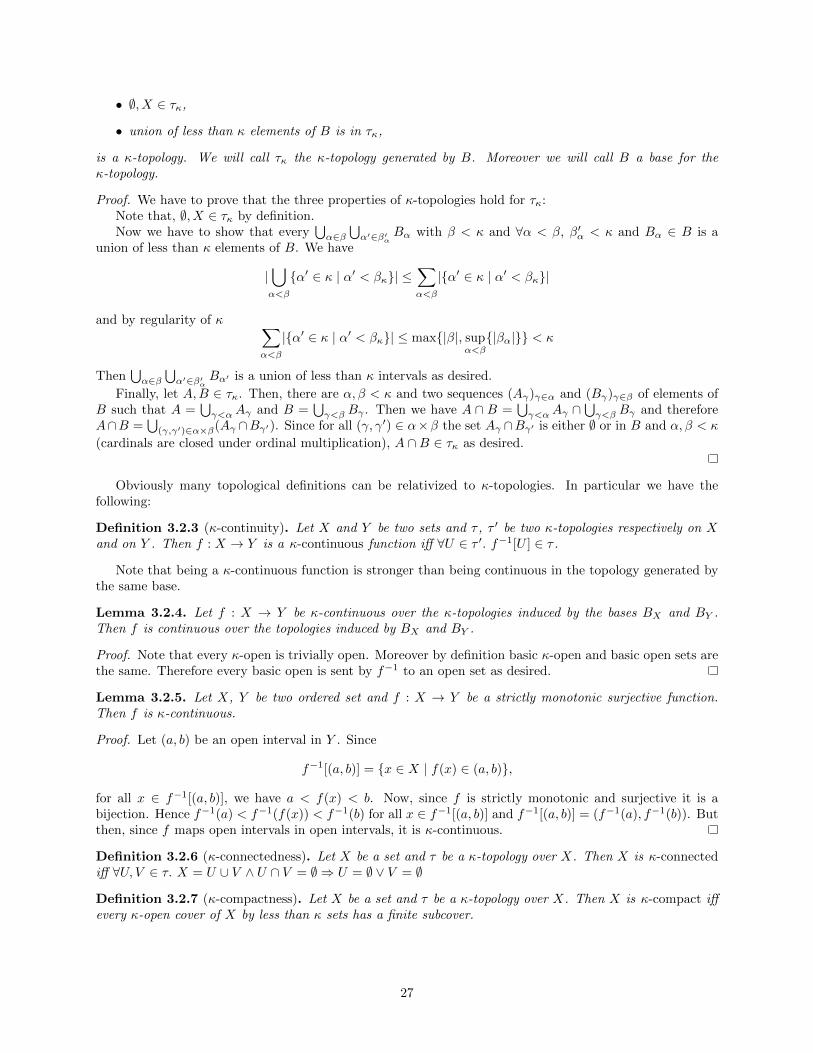
• ∅, X ∈ τκ,

• union of less than κ elements of B is in τκ,

is a κ-topology. We will call τκ the κ-topology generated by B. Moreover we will call B a base for theκ-topology.

Proof. We have to prove that the three properties of κ-topologies hold for τκ:Note that, ∅, X ∈ τκ by definition.Now we have to show that every

⋃α∈β

⋃α′∈β′α

Bα with β < κ and ∀α < β, β′α < κ and Bα ∈ B is aunion of less than κ elements of B. We have

|⋃α<β

{α′ ∈ κ | α′ < βκ}| ≤∑α<β

|{α′ ∈ κ | α′ < βκ}|

and by regularity of κ ∑α<β

|{α′ ∈ κ | α′ < βκ}| ≤ max{|β|, supα<β{|βα|}} < κ

Then⋃α∈β

⋃α′∈β′α

Bα′ is a union of less than κ intervals as desired.

Finally, let A,B ∈ τκ. Then, there are α, β < κ and two sequences (Aγ)γ∈α and (Bγ)γ∈β of elements ofB such that A =

⋃γ<αAγ and B =

⋃γ<β Bγ . Then we have A ∩ B =

⋃γ<αAγ ∩

⋃γ<β Bγ and therefore

A∩B =⋃

(γ,γ′)∈α×β(Aγ ∩Bγ′). Since for all (γ, γ′) ∈ α×β the set Aγ ∩Bγ′ is either ∅ or in B and α, β < κ

(cardinals are closed under ordinal multiplication), A ∩B ∈ τκ as desired.

Obviously many topological definitions can be relativized to κ-topologies. In particular we have thefollowing:

Definition 3.2.3 (κ-continuity). Let X and Y be two sets and τ , τ ′ be two κ-topologies respectively on Xand on Y . Then f : X → Y is a κ-continuous function iff ∀U ∈ τ ′. f−1[U ] ∈ τ .

Note that being a κ-continuous function is stronger than being continuous in the topology generated bythe same base.

Lemma 3.2.4. Let f : X → Y be κ-continuous over the κ-topologies induced by the bases BX and BY .Then f is continuous over the topologies induced by BX and BY .

Proof. Note that every κ-open is trivially open. Moreover by definition basic κ-open and basic open sets arethe same. Therefore every basic open is sent by f−1 to an open set as desired.

Lemma 3.2.5. Let X, Y be two ordered set and f : X → Y be a strictly monotonic surjective function.Then f is κ-continuous.

Proof. Let (a, b) be an open interval in Y . Since

f−1[(a, b)] = {x ∈ X | f(x) ∈ (a, b)},

for all x ∈ f−1[(a, b)], we have a < f(x) < b. Now, since f is strictly monotonic and surjective it is abijection. Hence f−1(a) < f−1(f(x)) < f−1(b) for all x ∈ f−1[(a, b)] and f−1[(a, b)] = (f−1(a), f−1(b)). Butthen, since f maps open intervals in open intervals, it is κ-continuous.

Definition 3.2.6 (κ-connectedness). Let X be a set and τ be a κ-topology over X. Then X is κ-connectediff ∀U, V ∈ τ. X = U ∪ V ∧ U ∩ V = ∅ ⇒ U = ∅ ∨ V = ∅

Definition 3.2.7 (κ-compactness). Let X be a set and τ be a κ-topology over X. Then X is κ-compact iffevery κ-open cover of X by less than κ sets has a finite subcover.

27

All these definitions behave quite well. Indeed, one can prove many relativized version of basic resultsfrom topology (see [1]). However, there are theorems from classical topology that do not transfer to κ-topologies. Typically in κ-topologies local properties do no transfer to global properties (e.g. in κ-topologiesopenness is not implied by local openness).

Now we will introduce a κ-topological analogous of the interval topology over an ordered set.

Definition 3.2.8 (Interval κ-Topology). Let X be an ordered set and B be the set of open intervals withend points in X ∪ {+∞,−∞}. We will call interval κ-topology over X the κ-topology generated by B.

From now on we will consider the interval κ-topology as the standard κ-topology over κ-real extensionsof R.

As we have seen, in order to be able to prove some basic theorems from analysis we need to work withina connected space. However, as we have already pointed out, we can not aim for connectedness of κ-realextensions of R. The next result is due to Alling [1] and it makes precise the connection between the densityof an ordered set and the connectedness of its interval κ-topology.

Theorem 3.2.9 (Alling). Let X be an ηκ-set endowed with the interval κ-topology and X ′ a subset of X.Then X ′ is κ-connected iff X ′ is an interval in X.

In view of Theorem 3.2.9, it is natural to require:

REQUIREMENT R4: Rκ has to be an ηκ-set.

Definition 3.2.10. Let K be a κ-real extension of R. Then K is super dense iff K is an ηκ-set.

For super dense κ-real extensions of R we have:

Corollary 3.2.11. Let K be a super dense κ-real extension of R. Then the interval κ-topology over K isκ-connected.

Theorem 3.2.12 (Alling). Let X be an ηκ-set and X ′ an interval in X. Then, if one of the following holds:

• Cof(X ′) = 1 or Cof(X ′) ≥ κ.

• Coi(X ′) = 1 or Coi(X ′) ≥ κ.

The interval κ-topology over X ′ is κ-compact.

Then we have:

Corollary 3.2.13. Let K be a super dense κ-real extension of R and [r, r′] be a closed interval of K. Then[r, r′] is κ-compact.

As in classical topology we have that κ-continuous functions preserve κ-connectedness and κ-compactness.

Theorem 3.2.14. Let f : X → Y be a κ-continuous function. If X is κ-connected then f(X) is κ-connected.

Proof. Assume f(X) not κ-connected. Therefore there are U, V κ-open subsets of Y which partition f(X).By the κ-continuity of f we have that f−1(U) and f−1(V ) are κ-open subsets of X. Moreover, sincef(X) = U ∪ V we have that f−1(U) and f−1(V ) separates X, but this contradicts our hypothesis thereforef(X) is κ-connected.

Theorem 3.2.15. Let f : X → Y be a κ-continuous function. If X is κ-compact then f(X) is κ-compact.

Proof. Take {Aβ}β<α with α < κ be a κ-open cover of f(X). By κ-continuity {f−1(Aβ)}β<α is a κ-opencover of X. Now since X is κ-compact there is a finite subcover A′ of A, but then A′ is the finite subcoverof f(X) we where looking for.

Given a κ-topological space (X, τ) and a subset Y of X, the κ-topology τ induces a κ-topology over Ythen, by analogy with classical topology we will call subspace κ-topology.

28

Lemma 3.2.16. Let X be a set, τ be a κ-topology over X and Y be a subset of X. Then the set τs definedas follows:

τs = {U ∩ Y | U ∈ τ},

is a κ-topology. We will call τs the subspace κ-topology of Y .

Proof. We will prove that the properties of κ-topologies holds on τs:Trivially ∅ ∈ τs. Moreover, since X ∈ τ , we have that Y ∈ τs.Let {Aβ}β∈α with α < κ be a family of elements of τs. Then for all β ∈ α there is an κ-open set Uβ in τ

such that Aβ = Uβ ∩ Y . Now, since⋃β∈αAβ =

⋃β∈α(Uβ ∩ Y ) = (

⋃β∈α Uβ) ∩ Y and (

⋃β∈α Uβ) is κ-open

in τ , we have that⋃β∈αAβ is κ-open in τs.

Let {Ai}i<n with n ∈ N be a finite family of κ-open sets in τs. For every i < n we have Ai = Ui ∩ Ywith Ui ∈ τ . Therefore we have

⋂i<nAi = (

⋂i<n Ui ∩ Y ) = (

⋂i<n Ui)∩ Y . Now, since

⋂i<n Ui is κ-open in

τ , we have that (⋂i<nAi) is κ-open in τs as desired.

It turns out that it is not true that the subspace κ-topology of an ordered set coincide with the κ-intervaltopology in general. But if we consider convex subsets, then interval κ-topologies and subspace κ-topologiescoincide.

Lemma 3.2.17. Let X be an ordered set and Y ⊂ X such that for all y1, y2 ∈ Y if there is y1 < x < y2 inX then x ∈ Y . Then the interval κ-topology over Y coincides with the subspace κ-topology over Y .

Proof. Let (a, b) be an open interval with end points in Y ∪ {+∞,−∞}. Since Y is convex, we have that(a, b) is an open interval in the order κ-topology over X. Therefore (a, b) ∩ Y = (a, b) is κ-open in thesubspace topology over Y . On the other hand let U = (a, b) ∩ Y with (a, b) a κ-open interval in X. Weclaim that U = {y ∈ Y | a < y < b} is either the empty set or an interval in Y . Indeed, since Y is convex, ify 6∈ Y then y is either a lower or an upper bound of Y . If {y ∈ Y | a < y < b} = ∅ then it is κ-open in theκ-subspace topology over Y . If {y ∈ Y | a < y < b} 6= ∅ then we have the following cases:

• a, b ∈ {y ∈ Y | a < y < b}: then U is an open interval in Y .

• a ∈ {y ∈ Y | a < y < b} and b /∈ {y ∈ Y | a < y < b}: then (a,+∞) = Y ∩ (a, b) and (a,+∞) is κ-openin Y .

• a 6∈ {y ∈ Y | a < y < b} and b ∈ {y ∈ Y | a < y < b}: then (−∞, b) = Y ∩ (a, b) and (a,+∞) is κ-openin Y .

• a, b 6∈ {y ∈ Y | a < y < b}: then (−∞,+∞) = Y ∩ (a, b) and (a,+∞) is κ-open in Y .

Then (a, b) ∩ Y is κ-open in the κ-subspace topology over Y .

3.3 Analysis Over Super Dense κ-real Extensions of RBy the results from the previous section we can modify the standard topological proof of the IVT to showthat its restriction to κ-continuous functions holds over super dense κ-real extensions of R.

Theorem 3.3.1 (IVTκ). Let K be a super dense κ-real extension of R, the set [a, b] ⊂ K be a closedsubinterval of K and f : [a, b] → K be a κ-continuous function. Then for every r ∈ K such that r is inbetween f(a) and f(b), there is c ∈ [a, b] such that f(c) = r.

Proof. We can assume f(a) 6= r 6= f(b). Assume that there is no c ∈ [a, b] such that f(c) = r. We definetwo sets:

A = f([a, b]) ∩ (−∞, r) and B = f([a, b]) ∩ (r,+∞).

They are non empty and disjoint (f(a) ∈ A and f(b) ∈ B). By definition they are also κ-open sets inf([a, b]). Moreover, since there is no c such that f(c) = r, we have that f([a, b]) = A ∪ B. Hence Aand B separates f([a, b]). Now by Theorem 3.2.9, [a, b] is κ-connected and by Theorem 3.2.14, f([a, b]) isκ-connected. Therefore we have a contradiction since we have shown that A and B separate f([a, b]) andf([a, b]) is κ-connected.

29

The next theorem we want to prove is the extreme value theorem over super dense κ-real extensions ofR. One of the main features of R on which the classical topological proof of the EVT depends on is the factthat if the image of a closed interval [a, b] of R under a continuous function f has no maximum then

{(−∞, a′) | a′ ∈ f([a, b])},

is a covering of f([a, b]). This fact is not true in general for κ-continuous functions and κ-open covers of sizeless than κ. In particular, if the cofinality of f([a, b]) is bigger than or equal to κ, then

{(−∞, a′) | a′ ∈ f([a, b])},

would not be a κ-cover of f([a, b]). For this reason we restrict ourself to a subclass of functions which preservethese κ-open covers.

Definition 3.3.2 (κ-super continuity). Let f : X → Y be a κ-continuous function. Then f is a rightκ-super continuous function iff for every close interval [a, b] in X, we have that Cof(f([a, b])) < κ. Moreoverf is a left κ-super continuous function iff for every close interval [a, b] in X, we have that Coi(f([a, b])) < κ.We will say that f is κ-super continuous if it is both left and right κ-super continuous.

Now we have all the notions we need to prove the EVT over super dense κ-real extensions of R.

Theorem 3.3.3 (EVTκ). Let K be a super dense κ-real extension of R, the set [a, b] be a closed interval ofK and f : [a, b]→ K be a right (left) κ-super continuous function. Then there is a point c ∈ [a, b] such thatf(c) is maximum (minimum) in f([a, b]).

Proof. Let A = f([a, b]). Assume that A has no maximum. Consider the following set:

{(−∞, a) | a ∈ A}.

By right κ-super continuity of f we have Cof(A) < κ, therefore there are α < κ and a sequence {ai}i<αin A which is cofinal in A. Hence, the set

{(−∞, ai) | i < α}

is a κ-open cover of A with less than κ intervals. Since [a, b] is a closed interval it is κ-compact and since fis κ-continuous A is κ-compact. Therefore there is a finite κ-open subcover A′ of A. Take M = maxA′, wehave that M ∈ f([a, b]) and M would be the maximum in f([a, b]). But this contradicts our assumption.

We end this section with some interesting properties of κ-continuous functions over super dense κ-realextensions of R.

It is a well-known fact that in every real closed field the IVT holds for polynomials in one variable (see[20, Theorem 3.3.9]), therefore it is natural to ask if polynomials over super dense κ-real extensions of R areκ-continuous. We have the following result:

Theorem 3.3.4. Let K be a super dense κ-real extension of R and p be a polynomial in one variable withcoefficients in K. Then p is κ-continuous.

Proof. Let p be a polynomial in K and (a, b) be an interval with endpoints in K ∪ {+∞,−∞}. Note thatsince constant functions are κ-continuous we can assume that p is not the zero polynomial. Since K is a realclosed field, the polynomials p(x) − a and p(x) − b have finitely many (possibly 0) roots in K. Let (ri)i∈nbe the strictly increasing listing of these roots. Define the set I as follows:

• if n = 0:

I =

{{(−∞,+∞)} If there is x ∈ K s.t. p(x) ∈ (a, b),

{∅} otherwise..

• If n > 0: define I as follows:

– (ri, ri+1) ∈ I iff p( ri+1−ri2 ) ∈ (a, b).

30

– (−∞, r0) ∈ I iff p(r0 − 1) ∈ (a, b).

– (rn−1,+∞) ∈ I iff p(r0 + 1) ∈ (a, b).

Now we claim that p−1[(a, b)] =⋃I. We will first prove that p−1[(a, b)] ⊆

⋃I.

Let x ∈ p−1[(a, b)]. If n = 0 then trivially x ∈ (−∞,+∞) =⋃I. Assume n > 0. We have the following

cases:Assume that there is i < n such that ri < x < ri+1, we want to prove p( ri+1−ri

2 ) ∈ (a, b). Assume not.Since, K is a real closed field, by [20, Theorem 3.3.9] , the IVT holds for polynomials. In particular, sincep( ri+1−ri

2 ) 6∈ (a, b) and p(x) ∈ (a, b) either p(x) − a or p(x) − b has a root in between ri and ri+1. But

this is in contradiction whit the fact that (ri)i∈n was strictly increasing. Therefore p( ri+1−ri2 ) ∈ (a, b) and

(ri, ri+1) ⊆⋃I.

Assume that for every i < n, we have x < ri. We want to prove p(r0 − 1) ∈ (a, b). Assume not. Asbefore the IVT holds for polynomials in K. In particular, since p(r0 − 1) 6∈ (a, b) and p(x) ∈ (a, b) eitherp(x)− a or p(x)− b has a root in between −∞ and r0. But this is in contradiction whit the fact that (ri)i∈nwas the strictly increasing listing of all the roots of p(x) − a and p(x) − b. Therefore p(r0 − 1) ∈ (a, b) and(−∞, r0) ⊆

⋃I.

Finally if for every i < n we have x > ri, then the proof is similar to the previous case.Note that the case in which x = ri for some ri is impossible since p(x) ∈ (a, b).Now we will prove that p−1[(a, b)] ⊇

⋃I. Let x ∈

⋃I. If n = 0, then there is y ∈ K such that

p(y) ∈ (a, b). Now, since the IVT hold for polynomials, if p(x) /∈ (a, b) we would have that either p(x) − aor p(x) − b has a root. This contradicts the assumptions. Assume n > 0. We will only consider the casein which x ∈ (ri, ri+1) for some i < n and p( ri+1−ri

2 ) ∈ (a, b). The other cases can be proved similarly. Wewant to prove that p(x) ∈ (a, b). Assume not. Since the IVT hold for polynomials, we would have that eitherp(x)− a or p(x)− b has a root in between (ri, ri+1). But we assumed (ri)i∈n strictly increasing. Thereforep(x) ∈ (a, b) as desired. Therefore p−1[(a, b)] =

⋃I.

Now since I is a finite list of intervals with end points in K ∪ {−∞,+∞} we have that⋃I is κ-open.

Hence p−1[(a, b)] is κ-open and p is κ-continuous as desired.

So far, one could get the impression that everything straightforwardly generalizes from the standardtopological case to the case of κ-topologies. The following negative result can serve as a warning that onecannot just assume that everything works nicely.

Definition 3.3.5 (κ-continuity at a point). Let f : X → Y be a function and x ∈ X. Then we say that f isκ-continuous at x iff for every κ-open set V containing f(x) there is a κ-open set U containing x such thatf(U) ⊆ V .

Theorem 3.3.6. Let f : X → Y be a κ-continuous function. Then it is κ-continuous at every point x ∈ X.

Proof. Let f be a κ-continuous function, x be an element of X and V be a κ-open set containing f(x).By the κ-continuity of f , we have that f−1(V ) is κ-open. Therefore there are α < κ and open intervals{Uβ}β∈α in X such that f−1(V ) =

⋃β∈α Uβ . Since x ∈ f−1(V ) there is β ∈ α such that x ∈ Uβ and, since

f−1(V ) =⋃β∈α Uβ therefore f(Uβ) ⊂ V as desired.

Before we prove that there are functions which are κ-continuous at every point but not κ-continuous, wewant to consider an example of a non κ-continuous function:

Let K be a super dense κ-real extension of R. First of all we note that + : K×K → K is not κ-continuous(therefore not κ-super continuous). Let (a, b) be an open interval of K (without loss of generality we canassume a 6= −∞ and b 6= +∞). Hence we have

+−1[(a, b)] = {〈x, y〉 | x+ y ∈ (a, b)},

therefore+−1[(a, b)] =

⋃x∈K

⋃y∈(a−x,b−x)

{〈x, y〉}.

31

We claim that +−1[(a, b)] is not κ-open. By contradiction assume that +−1[(a, b)] is κ-open. Let Π1 and Π2

be the projections over K ×K. Since (a, b) is κ-open, Π2(+−1[(a, b)]) is κ-open. Hence Π2(+−1[(a, b)]) =⋃β<α(cβ , dβ) for some α < κ. Note that

∀β < α. dβ 6= +∞

and∀β < α. cβ 6= −∞,

otherwise a = −∞ or b = +∞. Since {cβ}β<α and {dβ}β<α have cardinality less than κ, they are boundedin K (this follows by the fact that K is an ηκ-set). Hence there is d such that

∀β ∈ α. d > dβ .

Take y = d and x = a+b−2d2 . We have that 〈x, y〉 ∈ +−1[(a, b)] (i.e., x + y = a+b

2 = a + b−a2 ) and

y /∈⋃β<α(cβ , dβ). Hence + : K ×K → K is not κ-continuous.

Note that if we restrict the addition to a subset of K of cardinality strictly less than κ, we obtain aκ-continuous function. Let X be a subset of K of cardinality less than κ. Define the restricted addition asfollows:

+X = +�X.

We claim that +X is κ-continuous. Let (a, b) be an interval of K. Since

+−1X [(a, b)] =⋃

(a′,b′)⊂X

(a′, b′)× (a− a′, b− b′),

therefore +−1X [(a, b)] is κ-open as desired.Now we are ready to prove that there are functions that are κ-continuous at every point but not κ-

continuous.

Theorem 3.3.7. Let K be a super dense κ-real extension of R. Then there exists a function f : K → Kwhich is κ-continuous at every point but not κ-continuous.

Proof. We have just shown that + is not κ-continuous. We will prove that + is κ-continuous at every point.Let x, y ∈ K. We will prove the claim only for x, y > 0 the other cases follows similarly. Without loss ofgenerality we can assume x < y. Let V be a κ-open set containing x+y. We have that V =

⋃β∈α(aβ , bβ) for

α < κ many open intervals in K with end points in K ∪ {∞,−∞}. Let (aβ , bβ) such that x+ y ∈ (aβ , bβ).Without loss of generality we can assume that aβ 6= −∞ and bβ 6= ∞. Take εa = aβ − (x + y) andεb = bβ − (x+ y). Now we have that

A = (x− εa2, x+

εb2

)× (y − εa2, y +

εb2

)

is κ-open and trivially 〈x, y〉 ∈ A. Moreover for all 〈x′, y′〉 ∈ A we have

x′ + y′ < x+εb2

+ y +εb2

= bβ

andx′ + y′ > x− εa

2+ y − εa

2= aβ ,

therefore x′ + y′ ∈ V as desired.

3.4 The Real Closed Field Rκ

We are now ready to define Rκ. Before we present our construction, let us list all the requirements we haveintroduced in the previous sections.

32

R1: Rκ has to be a real closed field extension of R. Since every real closed field is elementary equivalentto R, this requirement will guarantee that Rκ behaves similarly to R with respect to the order and tothe operations.

R2: |Rκ| = 2κ. This is due to the fact that our generalized theory of computable analysis would have tobe a starting point for the study of the theory of represented spaces of cardinality bigger than 2ℵ0 .

R3: w(Rκ) = κ. This is needed since when we will generalize the classical representations of R to Rκ wewill need a set that can play the role that the rationals played in the classical case.

R4: Rκ is an ηκ-set. As we saw in the previous sections, this is needed in order for IVTκ and EVTκtheorems to hold in Rκ.

A naive attempt to define such extension would be that of starting from κ endowed with the surreal operations(i.e., the Hessenberg operations) and try to repeat the standard construction of Zκ and Qκ. Then, we coulddefine Rκ as the Cauchy completion of Qκ obtaining a Cauchy closed field Rκ as we showed in Section 2.2.Unfortunately this approach does not work. This is due to the following theorem:

Theorem 3.4.1 (Sikorski). The field Qκ is Cauchy closed. In particular,

Rκ = Qκ .

Recall that Qκ is a set of equivalence classes of pairs of elements in Zκ, hence it has cardinality at mostκ. Therefore Rκ violates R2 and is not a good candidate for our purposes. This construction appeared forthe first time in a paper from Sikorski in 1948 [26] (see also [18] for a complete study of this approach).During the work of this thesis, the Sikorski’s construction has been re-discovered independently by Asperoand Tsapronis and by myself.

Recall from Section 2.3 that we have the following property of surreal numbers:

Theorem 3.4.2 (Alling). Let κ′ be a regular cardinal. Then No<κ′ is a real closed field.

In particular we have that No<κ is a real closed field. Moreover since κ > ω, we have that R ⊂ No<κ.This means that R1 holds for No<κ. It is not hard to prove that No<κ also satisfies R4. Indeed we have amore general result:

Proposition 3.4.3 (Folklore). Let κ′ be a cardinal such that Cof(κ′) = α. Then No<κ′ is a ηα-set.

Proof. Assume L,R ∈ No<κ′ such that |L|+ |R| < κ′. Then for every x ∈ L and y ∈ R we have |x|, |y| < κ′.But since Cof(κ′) = α, we have that `(L) = sup{|x| | x ∈ L} and `(R) = sup{|x| | x ∈ R} are both smallerthan κ′. But then Theorem 2.3.7 we have |[L|R]| ≤ max{l(L), l(R)} < κ′ which imply [L|R] ∈ No<κ′ asdesired.

Then we have:

Proposition 3.4.4. The field No<κ has the following properties:

1) |No<κ| = κ.

2) Cof(No<κ) = Coi(No<κ) = w(No<κ) = κ.

3) Coi(No+<κ) = κ.

Proof. 1) Since we assumed κ = κ<κ, the statement follows from the fact that No<κ is the set of sequencesof pluses and minuses of length less than κ.

2) Note that κ ⊂ No<κ is a cofinal subset of No<κ and −κ is a coinitial subset of No<κ. By regularity ofκ, Cof(No<κ) = Coi(No<κ) = κ. Moreover, note that every dense subset of No<κ has to be cofinal in No<κ,therefore w(No<κ) ≥ κ and since |No<κ| = κ, we have w(No<κ) = κ.

3) We know that No<κ is a real closed field. Consider the following sequence S = { 1α}α∈κ. The sequence

S is coinitial in No+<κ. Indeed, take x ∈ No+<κ. We can assume x < 1, therefore x = 1y with y ∈ No+<κ. Take

α < κ such that α > y (note that α exists since κ is cofinal in No<κ), then x > 1α > 0 and S is coinitial

33

in No+<κ. Now, since |S| = κ, therefore Coi(No+<κ) ≤ κ. Moreover, note that any subsequence S′ of No+<κof cardinality less than κ cannot be coinitial in No+<κ. Indeed, let S′ be such a sequence. Since No<κ is anηκ-set, if we take L = {0} and R = S′, there is x ∈ No<κ such that L < {x} < R. Trivially x ∈ No+<κ and{x} < S′. Hence S′ is not coinitial in No+<κ as desired. In conclusion Coi(No+<κ) = κ.

Proposition 3.4.4 tells us that No<κ has almost all the properties that we want from Rκ but is still toosmall.

A possible approach to this problem would be that of repeating the construction of R over the surrealnumbers starting from No<κ instead that on No<ω. In particular one can define Rs

κ as follows:

Rsκ = No<κ ∪D,

where D is the following set:

D = {p ∈ Noκ | ∀α < κ∃κ > β > α. p(β) 6= p(α)}.

The problem with this construction is that, in the classical proof, in order to prove that the surrealoperations behave correctly with respect to non eventually constant sequences of pluses and minuses, theDedekind completeness of R is fundamental (see [14, Chapter 4 Section C]). Since we know that Rκ can notbe Dedekind complete, a generalization of this proof can not work. Moreover, an alternative proof wouldrequire a characterization of the operations over the surreal numbers in terms of sequences of pluses andminuses2. Such a characterization is still missing in the theory of surreal numbers. This is partially due tothe fact that the semantics of pluses and minuses in the the surreal numbers is not purely positional (seeSection 2.3).

We can then define Rκ as the Cauchy completion of No<. In Section 2.2 we showed a standard wayof completing a real closed field. In this section we will take a different prospective. Since we are workingwithin No, we will not need to build any new number.

Recall from Section 2.2 that a cut over a group is a pair 〈L,R〉 of subsets of the group such that L < R.In view of the Simplicity theorem (Theorem 2.3.5), we know that every such cut identifies a unique surrealnumber. Moreover, we have seen in Section 2.2 that the Cauchy completion of a field can be defined in termsof closure under Cauchy cuts. For these reasons, we can define the Cauchy completion of No<κ within thesurreal numbers in a very natural way as follows:

Definition 3.4.5 (No<κ). We define No<κ as follows:

No<κ = No<κ ∪{x | x = [L|R] where 〈L,R〉 is a Cauchy cut in No<κ}.

Now we will show that No<κ is a super dense κ-real extension of R. First of all we will prove that No<κis a dense subfield of No<κ and that No<κ is Cauchy complete (i.e., it is a Cauchy completion of No<κ).

Lemma 3.4.6. The field No<κ is dense in No<κ.

Proof. Let x, y ∈ No<κ be such that x < y. We can assume that at least one between x and y is not in No<κ,otherwise the statement follows trivially by the density of No<κ. Without loss of generality assume y is notin No<κ. Let [Lx|Rx] be the standard representation of x and [Ly|Ry] be a representation of y such that〈Ly, Ry〉 is Cauchy. Since x < y, by [14, Theorem 2.5] we have {x} < Ry and {y} > Lx. Moreover, sincex 6= y, by [14, Theorem 2.6] we have that either there exists xR ∈ Rx such that y ≥ xR or exists yL ∈ Lxsuch that yL ≥ x.

Assume that there is xR ∈ Rx such that y ≥ xR. Since yL /∈ No<κ and y 6= xR, we have y > xR > xas desired. On the other hand if there exists yL ∈ Lx such that yL ≥ x, then by the fact that Ly has nomaximum we can take y > y′L > yL ≥ x. Therefore y′L is the desired element of No<κ.

Lemma 3.4.7. The set No<κ is Cauchy closed.

2Note that all the operations over surreal numbers are defined in terms of their representations. It is not clear how and ifthese operations can be defined directly over surreal numbers.

34

Proof. Let 〈L,R〉 be Cauchy. We claim that there are two sequences (`γ)γ∈α and (rγ)γ∈β of elements ofNo<κ with α, β ≤ κ, which are respectively mutually cofinal in L and mutually coinitial in R. Moreover,since L has no minimum and R has no maximum, we can choose (`γ)γ∈α and (rγ)γ∈β such that `γ < rγ′

for all γ ∈ α and γ′ ∈ β. Let ` ∈ L and r ∈ R be two elements respectively of L and R. Since L has nomaximum and R has no minimum there exist `′ ∈ L and r′ ∈ R such that ` < `′ and r′ < r. By the densityof No<κ in No<κ there are `0, r0 ∈ No<κ such that ` < `0 < `′ < r′ < r0 < r. Now let 0 < γ < κ and assumewe have already defined `γ′ , for every γ′ < γ. We will define `γ , the same argument works for rγ . We havetwo cases:

• if there exists ` ∈ L such that `γ′ < ` for all γ′ < γ, then take `′ ∈ L such that ` < `′ and `γ ∈ No<κsuch that ` < `γ < `′.

• If for all ` ∈ L there is γ′ < γ such that `γ′ < `, then stop.

Now let α be the smallest ordinal on which the previous definition stops. Note that trivially α ≤ |L| ≤ κ.It is an easy induction to prove that for every γ < α there are `, `′ ∈ L such that ` < `γ < `′ and that forevery ` ∈ L there is γ ∈ α such that ` ≤ `γ . Therefore (`γ′)γ′<α is mutually cofinal with L as desired.

Now by [14, Theorem 2.3] we have [⋃γ∈α{`γ} |

⋃γ∈β{rγ}] = [L|R]. Moreover, since 〈L,R〉 is Cauchy, also

〈⋃γ∈α{`γ},

⋃γ∈β{rγ}〉 is Cauchy in No<κ. Finally, since [L|R] ∈ No<κ, we have that [

⋃γ∈α{`γ} |

⋃γ∈β{rγ}]

is in No<κ as desired.

Now we want to prove that our completion of No<κ is an ordered field. Before we can do that we needthe following lemma:

Lemma 3.4.8. Let y ∈ No+

<κ and [L|R] be a representation of y such that 〈L,R〉 is a Cauchy cut. We have:

∃ε0 ∈ No+

<κ∃c ∈ L \ {0}∀ε ∈ No+

<κ.

(ε < ε0)→ ∃yL ∈ L∃yR ∈ R. (yL + ε > yR ∧ yL > c).

Proof. By contradiction assume:

∀ε0 ∈ No+

<κ∀c ∈ L\{0}∃ε ∈ No+

<κ.

(ε < ε0 ∧ ∀yL ∈ L∀yR ∈ R. yL + ε > yR)→ yL ≤ c.

Choose ε0 > 0 such that the set X = {x ∈ L | x < y−ε0} 6= ∅. Note that ε0 exists since L has no maximum.Let c ∈ X. Since No is a real closed field we have c + ε0 < y. Now by density of No<κ we can choose0 < ε < ε0. Since 〈L,R〉 is a Cauchy cut, there are yL ∈ L and yR ∈ R such that yL + ε > yR. Hence yL ≤ cand ε < ε0 imply yL + ε < c+ ε < y < yR which is a contradiction.

Theorem 3.4.9. The set No<κ is a field.

Proof. Note that by density of No<κ in No<κ every time we need to prove a statement of the form

∀ε ∈ No+

<κ∃y ∈ Y. y < ε,

we can prove∀ε ∈ No+<κ ∃y ∈ Y. y < ε

instead.We only need to show the closure properties since we already know from the theory of surreal numbers

that the operations respect the ordered field axioms.+: let x, y ∈ No<κ. Note that since No<κ is a real closed field we can assume that at least one of the

two elements is not in No<κ. Without loss of generality we assume y 6∈ No<κ (the proof for x 6∈ No<κ isanalogous). We want to prove that x + y is represented by a Cauchy cut. Let us recall the definition of +over surreal numbers:

x+ y = [Lx + y, x+ Ly|Rx + y, x+Ry].

35

Recall that by uniformity of plus, we can use any representation for y, in particular we can assume thatwe used a representation of y induced by a Cauchy cut. Let ε ∈ No+<κ. Since y is represented by a Cauchycut [Ly|Ry], there exist yL ∈ Ly and yR ∈ Ry such that yL + ε > yR. Hence, since plus over surreal respectsthe axioms of real closed field theory, we have x+ yL + ε > x+ yR. Now x+ yL is on the left side of x+ yand x+ yR is on the right side, therefore x+ y is represented by a Cauchy cut as desired.·: As before we will assume x, y ∈ No<κ and y /∈ No<κ. First we recall the definition of x · y:

x · y = [Lx · y + x · Ly − Lx · Ly, Rx · y + x ·Ry −Rx ·Ry|Lx · y + x ·Ry − Lx ·Ry, Rx · y + x · Ly −Rx · Ly].

As before by uniformity of ·, we can assume that we used a representation of y induced by a Cauchy cut.Given ε ∈ No+<κ, we will prove that there exist xL, yL and yR such that

xL · y + x · yL − xL · yL + ε > xL · y + x · yR − xL · yR.

Note that it is enough to prove x · yL − xL · yL + ε > x · yR − xL · yR. Let xL be any element on the left inthe representation of x. Since x > x′ we have x − xL > 0, we can take ε′ = ε

x−xL . Moreover ε > 0 impliesε′ > 0. Now y was represented by a Cauchy gap therefore there exist yL and yR, respectively left and rightelements of a representation, such that yL + ε′ > yR. We have

(x− xL) · (yL + ε′) > (x− xL) · yR

andx · yL − xL · yL + ε > x · yR − xL · yR

as desired.−: let y ∈ No<κ and y /∈ No<κ. Recall that if [L|R] is a representation of y, therefore [−R| − L] is a

representation for −y. As before we can take a Cauchy representation of y. Let ε ∈ No+<κ. Hence, thereexist yL and yR such that yL + ε > yR. Therefore yL > yR − ε and −yR + ε > −yL as desired.

1y : let y ∈ No<κ and y /∈ No<κ. By the definition of 1

y it is not hard to see that 1yR

and 1yL

are respectively

left and right members of the representation of 1y . Now by Lemma 3.4.8 there exist ε0 ∈ No+<κ and c > 0

such that for every ε ∈ No+<κ such that ε < ε0 there are yL and yR such that yL + ε > yR and yL > c.Therefore we have the following:

1

yL− 1

yR< ε⇔ yR − yL

yL · yR< ε.

Now, by the fact that y has a Cauchy representation, we can choose yR − yL arbitrary small. Moreover,since yR−yL

yL·yR < yR−yLc2 , it is enough to take ε′ = ε · c2 and yL + ε′ > yR to get

1

yR− 1

yL< ε

as desired.

Now we want to prove that No<κ is a real closed field. Before we can do that we need to prove that

polynomial over No<κ are continuous with respect to the interval topology over No<κ. Note that the followinglemma is true in general for ordered fields:

Lemma 3.4.10. Let f : No<κ → No<κ and g : No<κ → No<κ be two continuous functions. Then f + g andf · g are continuous.

Proof. Note that since f × g is continuous, f + g = + ◦ (f × g) and f · g = · ◦ (f × g), we only need to prove

that sum and product over No<κ are continuous. Let (a, b) be an open interval in No<κ. We have that

+−1[(a, b)] = {〈x, y〉 ∈ No<κ × No<κ|x+ y ∈ (a, b)},

therefore a < x+ y < b. Moreover, since No<κ is an ordered field, a− y < x < b− y. Now we have

+−1[(a, b)] =⋃

(a′,b′)⊂No<κ

(a′, b′)× (a− a′, b− b′)

36

therefore + is continuous in No<κ. A similar reasoning works for ·. Let (a, b) be an open interval in No<κ,we have that

·−1[(a, b)] = {〈x, y〉 ∈ No<κ × No<κ | x · y ∈ (a, b)},

therefore a < x · y < b. We will only prove that case x, y > 0, the other cases follows similarly. Since No<κis an ordered field, a

y < x < by and

·−1[(a, b)] =⋃

(a′,b′)⊆No<κb′ 6=0

(a′, b′)× (a

a′,b

b′),

therefore · is continuous as desired.

Now it is easy to see that every polynomial over No<κ is continuous.

Theorem 3.4.11. Let p(x) be a polynomial with coefficients in No<κ. Then p is continuous.

Proof. By induction over the degree of p(x). Note that every constant function is trivially continuous.Moreover if p(x) is of degree n+ 1 then

p(x) =

i=n∑i=0

aixi = x(

i=n∑i=1

aixi−1) + a0.

Let p′(x) =∑i=ni=1 aix

i−1), it is continuous by inductive hypothesis. Moreover p = (id · p′) + ca0 where ca0 isthe constant function with value a0. Hence by the previous lemma we have that p is continuous.

Finally we are ready to prove that No<κ is a real closed field.

Theorem 3.4.12. The field No<κ is real closed.

Proof. It is enough to show that No<κ is an elementary substructure of No<κ with respect to the language ofreal closed field theory, (+, ·, 0, 1, <). We will prove that the Tarski-Vaught test holds. Let φ(x) be a formulain one variable with parameters in No<κ. Note that, since No<κ is a real closed field, for any formula of thistype there are (pi)i∈n and (qi)i∈m with m,n ∈ N and pi,qi polynomials in No<κ such that

φ(x)⇔∧i∈n

pi(x) = 0 ∧∧i∈m

qi(x) > 0.

Now let b ∈ No<κ be such that φ(b) holds. If there is i < n such that pi is not the trivial zero polynomial,then pi(b) = 0 and b is algebraic over No<κ. But since No<κ is a real closed field, it has no proper orderedalgebraic extensions, therefore b ∈ No<κ. If for all i the polynomial pi is the zero polynomial, then b is a

solution of the system∧i∈m qi(x) > 0. Now every qi is continuous in No<κ hence there are ai 0 for all x ∈ (ai, ci). By the density of No<κ in No<κ, there are ai < a′i 0 for all x ∈ (a′i, c

′i). Take c = min{c′i | i ∈ m} and a = max{a′i | i ∈ m}. Hence, for every x ∈ (a, c)

we have∧i∈m qi(x) > 0 as desired. Then by the Tarski-Vaught test we have that No<κ is an elementary

substructure of No<κ. In conclusion, since No<κ is real closed, we have that No<κ is a real closed.

In particular the fact that No<κ is a real closed field makes the field satisfy all the first order propertiesvalid over R.

Now that we have shown that No<κ is a real closed field extending R we want to check that also all the

other properties of super dense extensions of R hold for No<κ.

Lemma 3.4.13. Let No≤κ be the set of surreal numbers of length at most κ. Then No<κ ⊆ No≤κ.

37

Proof. We will prove that No≤κ contains the Dedekind closure of No<κ. This implies by definition that

No≤κ also contains the Cauchy closure of No<κ, namely No<κ. Let 〈L,R〉 be a cut in No<κ, we claim that[L|R] ∈ No≤κ. Note that for every x ∈ L ∪ R, since L ∪ R ⊂ No<κ, |x| < κ. Hence, by Theorem 2.3.7 we

have |[L|R]| ≤ κ. Then [L|R] ∈ No≤κ as desired. Since No<κ = No<κ ∪C where C is the set of Cauchy cuts

therefore No<κ ⊆ No≤κ as desired.

Theorem 3.4.14. The real closed field No<κ has the following properties:

1) Deg(No<κ) = κ

2) No<κ is an ηκ-set.

3) |No<κ| = 2κ, Cof(No<κ) = Coi(No<κ) = w(No<κ) = κ.

Proof. 1) We will prove that Deg(No<κ) = Deg(No<κ). Since No<κ is dense in No<κ, then we have that

Deg(No<κ) ≥ Deg(No<κ). Now, assume that every sequence of length κ in No<κ is such that there is

x ∈ No+

<κ smaller than every element of the sequence. Then, by the density of No<κ, there is x′ ∈ No<κsuch that 0 < x′ < x, but this is absurd because Deg(No<κ) = κ.

2) Take L,R ⊂ No<κ such that |L|+ |R| < κ and L < R. We have the following possibilities:

• L has no maximum and R has no minimum: by the density of No<κ in No<κ, as in the proof ofLemma 3.4.7, there are two sequences (`γ)γ∈α and (rγ)γ∈β with α, β < κ of elements of No<κ whichare respectively cofinal in L and and coinitial in R and such that

∀α′ ∈ α∀β′ ∈ β. `α′ < rβ′ .

Hence, since No<κ is an ηκ-set, we have that there is x ∈ No<κ such that L < {x} < R as desired.

• L has maximum M and R has minimum m: it is enough to take x = m−M2 .

• L has maximum M and R has no minimum: consider the sequence (r −M)r∈R. Note that

∀r ∈ R. r −M > 0,

therefore, since Deg(No<κ) = κ and |R| < κ there is x ∈ No<κ such that ∀r ∈ R. 0 < x < r −M butthen M < x+M and ∀r ∈ R.x+M < r as desired.

• L has no maximum M and R has minimum m: a proof similar to the previous case applies.

3) Note that by the construction of No<κ, since No<κ is a dense subfield of No<κ, we have

Cof(No<κ) = Coi(No<κ) = w(No<κ) = κ.

Now, we want to prove 2κ ≤ |No<κ| ≤ 2κ. On the one hand, by Lemma 3.4.13 we have that No<κ ⊂ No≤κ.

Indeed, No≤κ contains the Dedekind completion of No<κ, hence also its Cauchy completion No<κ. Then,

since |No≤κ| = 2κ, we have that |No<κ| ≤ 2κ.On the other hand let {0, 1}<κ be the full binary tree of height κ, we define a tree T which is in bijection

with {0, 1}<κ and whose nodes are in No<κ×No<κ. We define the tree by recursion as follows:

let x0, y0 ∈ No<κ such that x0 < y0 < 1 set (x0, y0) as the root of the tree.

Assume that the tree is already defined for all β < α < κ, for every w ∈ {0, 1}α define xw and yw asfollows:

(A) yw − xw <1

α.

(B) xw′ < xw < yw < yw′ for all w′ ⊂ w.(C) (xw, yw) ∩ (xw′ , yw′) = ∅ for all w′ ∈ {0, 1}α, w′ 6= w.

38

Note that the tree is well defined since No<κ is an ηκ-set and every path from an element to the root hasstrictly less than κ elements. Now by property (B) and by the fact that No<κ is a real closed field, we havethe following:

∀p ∈ {0, 1}κ∀α < κ∀β > α. xp�β ∈ (xp�α, yp�α).

Moreover by construction for every p ∈ {0, 1}κ, the sequence (xp�α)α<κ is Cauchy. Indeed, let ε ∈ Q+κ . Take

α such that 1α ≤ ε. By (A) we have

yp�α − xp�α <1

α≤ ε

and∀β > α. xp�β ∈ (xp�α, yp�α).

Then, since No<κ is a real closed field,

∀β, β′ > α. |xp�β − xp�β′ | < xp�α − yp�α < ε

as desired.Finally we have that if p, p′ ∈ {0, 1}κ and p 6= p′ then (xp�α)α∈κ and (xp′�α)α∈κ converge to different

points. Let α be the least such that p(α) 6= p(α). Then by construction xp�α+1 and xp′�α+1 are such that

(xp�α+1, yp�α+1) ∩ (xp′�α+1, yp′�α+1) = ∅.

Now, since∀β > α. xp�β ∈ (xp�α+1, yp�α+1)

and∀β > α. xp′�β ∈ (xp′�α+1, yp′�α+1)

we havelimβ∈κ

xp�β ∈ (xp�α+1, yp�α+1)

andlimβ∈κ

xp′�β ∈ (xp′�α+1, yp′�α+1).

Hence limβ∈κ xp�β 6= limβ∈κ xp′�β as desired. Then we have 2κ ≤ |No<κ| as desired.

Therefore all the properties listed at the beginning of this section are fulfilled by No<κ. We are nowready to define our generalization of R.

Definition 3.4.15 (Rκ and Qκ). We define Rκ as follows:

Rκ = No<κ.

We will use +∞ and −∞ to denote respectively the least ordinal not in Rκ and its inverse namely +∞ = κand −∞ = −κ. Moreover we define:

Qκ = No<κ .

From now on, we will call κ-reals the elements of Rκ and κ-rationals the elements of Qκ.Note that the construction of Rκ we have just presented seems to be really different form the construction

of R within the theory of surreal numbers. The following theorems show some connection between thedefinition of R and Rκ.

Definition 3.4.16. Let x ∈ No be an eventually constant surreal number. We will call stabilization pointof x the smallest ordinal α such that ∀β ≥ α.x(α) = x(β).

Theorem 3.4.17 (Alling). A surreal number x ∈ No is in the Dedekind closure NoD<κ of No<κ iff one ofthe following holds:

39

• x ∈ No<κ.

• x ∈ Noκ and is not eventually constant.

• x ∈ Noκ and its stabilization point is a limit ordinal.

Since Rκ ⊂ NoD<κ, we have the following corollary:

Corollary 3.4.18. Let x ∈ Rκ. Then one of the followings holds:

1) x has length smaller than κ.

2) x has length κ but is not eventually constant.

3) x has length κ and its stabilization point is a limit ordinal.

Note that the converse is not true (i.e., there are elements that satisfies 2) or 3) which are not in Rκ). Itis still unclear if there is a characterization of Rκ similar to that of R (i.e., in terms of surreal numbers). Inparticular, we don’t know if the fact of being a limit of a Cauchy sequence can be characterized in terms ofsequences of pluses and minuses. We leave the following open question:

Open Question 3.4.19. Is there any characterization of Rκ in terms of sequences of pluses and minuses?

We conclude this chapter with some result on the interval topology and the interval κ-topology over Rκ.The first two results are a generalized version of a classical result over R.

Lemma 3.4.20. Every open interval of Rκ has cardinality 2κ.

Proof. Let (r, r′) ⊂ Rκ. On the one hand, since |Rκ| = 2κ, we have that |(r, r′)| ≤ 2κ. On the other hand, bythe same construction of the third point of Theorem 3.4.14, we can build a tree with root (r, r′) of Cauchysequences converging to different limits. Note that, since all the points of these Cauchy sequences are in(r, r′), their limits are also in (r, r′). Then we have 2κ ≤ |(r, r′)| as desired.

Theorem 3.4.21. Let τ be the interval topology over Rκ. Then the set of open intervals of Rκ with endpoints in Qκ ∪{+∞,−∞} is a base for τ .

Proof. It is enough to show that every open interval with end points in Rκ ∪{+∞,−∞} is a union openintervals with κ-rational end points. Let (a, b) an interval with end points in Rκ ∪{+∞,−∞}. If a = −∞and b = +∞ then trivially (a, b) has end points in Qκ ∪{+∞,−∞}. If a ∈ Rκ, and b = +∞ then bydensity of Qκ in Rκ, we have that (a, b) =

⋃q∈{Qκ|q>a}(q, b) (a similar argument proves the case a = −∞,

b ∈ Rκ). Finally if a, b ∈ Rκ then by density of Qκ there are q, q′ ∈ Qκ such that a < q < q′ < b. Then(a, b) =

⋃{q′′∈Qκ|q′′>a}(q

′′, q′) ∪⋃{q′′∈Qκ|q′′<b}(q, q

′′) as desired.

Note that the previous proof can not be used to prove that intervals with κ-rational end points are abase for the interval κ-topology over Rκ. In fact, since Rκ is an ηκ-set, in general we can not write intervals(a, b) with end points in Rκ ∪{+∞,−∞} as a union of less than κ open intervals with κ-rational end points.This is a consequence of the more general fact that κ-topologies depends on the cardinality of their bases.In general for κ-topology we have:

Lemma 3.4.22. Let B and B′ two bases for the topology τ over a set X. If B and B′ generate the sameκ-topology then (|B|)<κ = (|B′|)<κ.

Proof. Let B, B′ two bases for τ . Assume that they generate the same κ-topology τκ. By definition, wehave (|B|)<κ = |τκ| = (|B′|)<κ as desired.

Note that the other direction does not hold. Indeed, consider the topology generated by the set B ofopen intervals with end points in Rκ, and the topology generated by the base B′ = B ∪ {(1,+∞)}. It is nothard to see that the two bases both generates the interval topology over Rκ and that they have the samecardinality. But while (1,+∞) is κ-open in the κ-topology generated by B′ it is not κ-open in the κ-topologygenerated by B (recall that Cof(Rκ) = κ). The fact that Rκ is an ηκ-set gives us more information aboutthe interval κ-topology over Rκ.

40

Theorem 3.4.23. Let B be a base for the interval κ-topology τ over Rκ. Then |B| = 2κ.

Proof. First note that every base B of τ is of the form B = B′ ∪B′′ where

B′ ⊆ {(a, b) ⊂ Rκ | a, b ∈ Rκ ∪{+∞,−∞} ∧ a < b}

andB′′ ⊂ {O ⊂ Rκ | O κ− open in the interval κ-topology}.

Assume |B| < 2κ. Now, defineA = {a | (a, b) ∈ B′}

andA′ = {ai | O ∈ B′′ ∧O =

⋃β<α

(aβ , bβ) ∧ α < κ}.

Since |B| < 2κ, there exists r /∈ A ∪ A′. Consider the interval (r, r + 1). Since (r, r + 1) is an open intervalin Rκ and B is a base for the interval κ-topology, we have

(r, r + 1) =⋃β<α

Oβ ∪⋃β<α′

(aβ , bβ)

for some α, α′ < κ and Oβ ∈ B′′ such that for all β ∈ α and (aβ , bβ) ∈ B′ for all β ∈ α′. Now, take the sets{r} and (A ∩ (r, r + 1)) ∪ (A′ ∩ (r, r + 1)). We have

|(A ∩ (r, r + 1)) ∪ (A′ ∩ (r, r + 1))| < max{|α|, |α′|} < κ

and{r} < (A ∩ (r, r + 1)) ∪ (A′ ∩ (r, r + 1)).

But since Rκ is an ηκ-set, there exists x ∈ Rκ such that

{r} < {x} < (A ∩ (r, r + 1)) ∪ (A′ ∩ (r, r + 1)),

therefore we have x ∈ (r, r + 1) and x /∈⋃β<αOβ ∪

⋃β<α′(aβ , bβ) which is a contradiction.

The last theorem we prove in this section can be seen as an amalgamation theorem for κ-continuousfunctions. It will be a very useful tool to build κ-continuous functions.

Theorem 3.4.24. Let (xi)i∈n be a strictly increasing sequence in Qκ such that, defining (Xi)i∈n by:

Xi =

(−∞, x0] i = 0,

[xi, xi+1] 0 < i < n− 1,

[xn−1,+∞) i = n− 1,

we have Rκ =⋃i∈nXi. Then every function f : Rκ → Rκ such that f�Xi is κ-continuous for every 0 < i < n

is κ-continuous.

Proof. Let (a, b) be an open interval with end points in Rκ ∪{+∞,−∞}. Define U = f−1(a, b). We wantto prove that U is κ-open. For every 0 < i < n set Ui = U ∩ Xi. By κ-continuity of f�Xi, every Ui isκ-open in Xi. Then, for every i < n, there is Oi =

⋃α∈βi(a

iα, b

iα) such that Ui = Oi ∩Xi. Moreover note

that U =⋃i∈n Ui. We want to show that U is κ-open. To do that we will extract from (Ui)i∈n a sequence

(U ′i)i∈n such that U ′i is a union of less than κ κ-open intervals with end points in Rκ ∪{+∞,−∞} such thatU =

⋃i∈n U

′i . For every i < n we define U ′i as follows:

• if Ui = ∅ then Ui = U ′i .

• If for all α < βi (aiα, biα) ⊂ Xi then Ui = U ′i .

41

If none of the previous applies we define:

I = {(aiα, biα) | α < βi ∧ (aiα, biα) ⊂ Xi}.

Moreover we define a set I ′ as follows:

• for every (aiα, biα) such that (aiα, b

iα) ∩Xi = (aiα, xi+1]. Then a < f(xi+1) < b. We have two cases:

– If for all i < j ≤ n and for every x ∈ Xj we have f(x) ∈ (a, b). We have

U ⊇ (aiα,+∞) ⊇ (aiα, xi+1].

In this case (aiα,+∞) ∈ I ′.– If exists i < j ≤ n and there exists x ∈ Xi such that f(x) 6∈ (a, b). Then take m least of these j.

Hence, there is bm ∈ Xm such that f(bm) ∈ (a, b). Therefore

U ⊇ (aiα, bm) ⊇ (aiα, xi+1].

Note that we can pick bm 6= xi+1 because (a, b) is an open interval, therefore f(xi+1) 6= b andf�Xm is κ-continuous. In this case (aiα, bm) ∈ I ′.


iα) ∩Xi = [xi, b

iα). Then a < f(xi)) < b. We have can use the same

construction of the previous case.


iα) ∩Xi = [xi, xi+1]. By using the previous two cases with [xi, xi+1)

and (xi, xi+1], we can find (a′, b′) such that

U ⊇ (a′, b′) ⊃ [xi, xi+1]

and take (a′, b′) ∈ I ′.

Then we define U ′i = I ∪ I ′. Note that every U ′i is a κ-open set in Rκ.Now, note that, by the definition of {U ′i}i<n we have Ui ⊆ U ′i and Ui ⊂ U for every 0 < i < n. Hence

U =⋃i∈n U

′i and therefore U is κ-open as desired.

3.5 Generalized Descriptive Set Theory

Metrizability is one of the main ingredients of descriptive set theory. As we noticed in Section 2.4, sincegeneralized Baire space is not metrizable, all those notions from descriptive set theory that depend onmetrizability cannot be easily generalized to uncountable cardinals. In this section we will use Rκ to fill thisgap between classical and generalized descriptive set theory. In particular we will define a generalization ofmetrizability to κ which can be used to study generalized Baire space from a metric point of view. Then wewill show that, as in the classical case, κ-Borel sets form a hierarchy.

Note that in this section we will focus our attention on topologies rather than κ-topologies. This is dueto the following facts:

We want to use Rκ to generalize results from classical descriptive set theory to generalized Baire space.In descriptive set theory the topology over κκ plays a central role, the use of κ-topologies would then makeour work harder and sometimes impossible.

The results at the end of this section will be very important in Chapter 4 where we will be forced toconsider the standard topology over κκ.

Definition 3.5.1 (κ-metric Space). A κ-metric space is a pair (X, d) where X is a set and d : X → Rκ isa function such that:

• d(x, y) ≥ 0.

• d(x, y) = 0⇔ x = y.

42

• d(x, y) = d(y, x).

• d(x, y) + d(y, z) ≥ d(x, z).

We will call d a κ-metric. Moreover a κ-metric d is called a κ-ultrametric if the following hold:

d(x, z) ≤ max{d(x, y), d(y, z)}.

Given a κ-metric space (X, d), x ∈ X and r ∈ Rκ, we define

B(x, r) = {y | d(x, y) < r}

andB[x, r] = {y | d(x, y) ≤ r}.

We will call B(x, r) the open ball of centre x and radius r, and B[x, r] the closed ball of centre x and radiusr.

Note that the absolute value is definable in the language of real closed fields as follows:

|x| = y ⇔ (x ≥ 0→ y = x) ∧ (x < 0→ y = −x).

Now, since Rκ is a real closed field and the absolute value over R is a metric, the absolute value over Rκ isa κ-metric (note that all the properties required by metrics are sentences in (+, ·, 0, 1, <)).

Definition 3.5.2 (κ-metrizability). Let τ be a topology over X. Then τ is said to be κ-metrizable if thereis a κ-metric d : X → Rκ such that

B = {B(x, r) | x ∈ X and r ∈ Rκ}

is a base for τ . Moreover, we say that τ is completely κ-metrizable if every Cauchy sequence in X inducedby d has a limit in X.

As we have just seen, the classical metric over R extends naturally to a κ-metric for Rκ. It is not hardto see that the absolute value induces the interval topology over Rκ.

Theorem 3.5.3. The interval topology over Rκ is κ-metrizable.

Proof. We want to show that |·| : Rκ → Rκ induces the interval topology over Rκ. We will show that theset of open balls B is equal to the set of open intervals with end points in Rκ. Since Rκ is a real closed field,the proof is the same as in the classical case.

On the one hand let (r1, r2) be an open interval in Rκ. Then

B(r2 + r1

2,r2 − r1

2) = (r1, r2).

Indeed, we have:

x ∈ B(r2 + r1

2,r2 − r1

2)⇔ r2 + r1

2− r2 − r1

2< x <

r2 + r12

+r2 − r1

2⇔ r1 < x < r2

⇔ x ∈ (r1, r2).

On the other hand, let B(x, r) be an open ball, then trivially B(x, r) = (x− r, x+ r).In conclusion B is the set of open sets with end points in Rκ, hence B generates the interval topology

over Rκ

Proposition 3.5.4. Let (X, τ) be κ-metrizable and C be a closed subset of X. Then C is the intersectionof κ many open sets.

43

Proof. Let d be a κ-metric which induces τ and C a closed set. Define:

Cα = {x | ∃c ∈ C. d(x, c) <1

α}.

Note that for every α ∈ κ we have that Cα =⋃c∈C B(c, 1

α ) is open. We claim C =⋂α∈κ Cα.

On the one hand, assume x ∈ C. Then d(x, x) = 0 and x ∈ Cα for every α ∈ κ. Therefore x ∈⋂α∈κ Cα.

On the other hand if x ∈⋂α∈κ Cα then for all α ∈ κ there exists c ∈ Cα such that d(x, c) < 1

α . For eachα choose cα ∈ Cα ∩ C. Since limα∈κ

1α = 0, we have limα∈κ d(x, cα) = 0 and since C is closed, x ∈ C as

desired.

Analogously to the classical case, where ωω was completely metrizable, generalized Baire space can beproved to be completely κ-metrizable.

Theorem 3.5.5. The generalized Baire space κκ is completely κ-metrizable.

Proof. First we define the following κ-metric:

d(x, y) =

{0 iff x = y,1

α+1 α minimal s.t. x(α) 6= y(α),

for x, y ∈ κκ.We claim that d is a κ-metric:Trivially d(x, y) ≥ 0, moreover d(x, y) = 0 if and only if x = y and d(x, y) = d(y, x). We want to prove

the following:∀x∀y∀z.d(x, y) + d(y, z) ≥ d(x, z).

If d(x, y) = 0 or d(y, z) = 0 the statement follows trivially. Assume d(x, y) = 1α+1 , d(y, z) = 1

β+1 and

d(x, z) 6= 0, in particular d(x, z) = 1γ+1 . First assume α ≤ β. Since y�β = z � β and α ≤ β, we have that

d(x, z) = d(x, y) ≤ d(x, y) + d(y, z) as desired. Now assume β < α. Since x�α = y � α and β < α, we havethat d(x, z) = d(y, z) ≤ d(x, y) + d(y, z) as desired. Note that we actually proved that d is a κ-ultrametric.

Now we want to show that the set of open balls induced by d is a base for generalized Baire space.On the one hand let w ∈ κ<κ. We claim that

[w] = B(p,1

|w|+ 1) where w ⊂ p.

By definition we have

p′ ∈ [w]⇔ w ⊆ p′ ⇔ d(p, p′) <1

|w|+ 1⇔ p′ ∈ B(p,

1

|w|+ 1)

as desired. On the other hand let B(p, r) with r ∈ Rκ be an open ball. Note that by definition of d, we haveB(p, r) = B(p, 1

αr+1 ) with αr greatest ordinal such that 1αr+1 ≤ r. Now let w = p�αr as before. We have

p′ ∈ [w]⇔ w ⊂ p′ ⇔ d(p, p′) <1

|w|+ 1=

1

αr + 1⇔ p′ ∈ B(p,

1

αr + 1) = B(p, r)

as desired.Finally we want to prove that κκ is complete w.r.t. d. Let (pα)α∈κ a Cauchy sequence in κκ. Note that

∀ε ∈ R+κ ∃γ < κ∀α, α′ ≥ γ. d(pα, pα′) < ε.

Now, define the following sequence

p`�0 = 〈〉,

p`�α = pγ�α γ smallest s.t. ∀α, α′ ≥ γ. d(pα, pα′) <1

α.

44

Since the starting sequence was Cauchy, pγ always exists. We claim that (p`�α)α∈κ is monotone. Let α ≤ β.If p`�α = p`�β then trivially p`�α ⊆ p`�β. Hence assume p`�α 6= 〈〉 6= p`�β. Let γ and γ′ be such that

p`�α = pγ�α p`�β = pγ′�β.

Without loss of generality assume γ′ ≥ γ a similar proof works for γ′ < γ. By the definition we have

d(pγ , pγ′) <1

α+ 1,

and thereforep`�α = pγ�α ⊆ pγ′�β = p`�β

as desired. Then the sequence p` =⋃α∈κ p`�α is well defined.

Now we want to prove that limα∈κ pα = p`, that is

∀ε ∈ R+κ ∃γ < κ∀β ≥ γ. d(pβ , p`) < ε.

Fix ε ∈ R+κ . Let α such that 1

α+1 ≤ ε. We have that

p`�α = pγ�α,

with γ smallest ordinal such that

∀β, β′ ≥ γ. d(pβ , pβ′) <1

α+ 1

In particular, we have that

∀β ≥ γ. d(pβ , pγ) <1

α+ 1.

Then, since p`�α = pγ�α, we have that

∀β ≥ γ. d(pβ , p`) <1

α+ 1≤ ε,

therefore limα∈κ pα = p` as desired.

Definition 3.5.6 (κ-separability). Let τ be a topological space over X. Then τ is κ-separable iff it has adense subset of cardinality κ.

Since in the previous section we have proved that the set of intervals with end points in Qκ is a base forthe interval topology over Rκ, we have the following:

Proposition 3.5.7. The interval topology over Rκ is κ-separable.

Recall that we assumed κ<κ = κ, therefore the standard base of κκ is of cardinality κ. In particular wehave:

Proposition 3.5.8. The generalized Baire space κκ is κ-separable.

Polish spaces have a central role in descriptive set theory, it is natural then to generalize them touncountable cardinals.

Definition 3.5.9 (κ-Polish Space). Let τ be a topological space over X. Then, τ is κ-Polish iff it isκ-separable and completely κ-metrizable.

By what we have proved before, we have:

Corollary 3.5.10. The generalized Baire space κκ is κ-Polish.

Now we are ready to define the generalization to κ of the Borel hierarchy over κ-metrizable sets. First ofall we extend the notion of a Borel set to our generalized setting. The following definition can be found in[13], [21] and [15]:

45

Definition 3.5.11 (κ-Borel Sets). The collection B(X) of κ-Borel sets over a topological space (X, τ) isthe smallest containing the topology and closed under unions of size κ and complementation.

Since we have generalized metrizability to Rκ, we can now show that the κ-Borels form a hierarchy as inthe classical case.

Definition 3.5.12 (κ-Borel hierarchy). Let (X, τ) be a κ-metrizable space. Then for 1 < α < κ+ we define:

Σ(κ,0)1 (X) = open sets,

Π(κ,0)1 (X) = closed sets,

Σ(κ,0)α (X) = {

⋃β∈κ

Aβ | ∀β < κ∃γ < α. Aβ ∈ Π(κ,0)γ (X)},

Π(κ,0)α (X) = {

⋂β∈κ

Aβ | ∀β < κ∃γ < α. Aβ ∈ Σ(κ,0)γ (X)}.

As usual ∆(κ,0)α (X) = Σ

(κ,0)α (X) ∩Π

(κ,0)α (X).

Proposition 3.5.13. If (X, τ) is κ-metrizable, then for every α ∈ On we have Σ(κ,0)α (X) ⊆ Σ

(κ,0)α+1 (X) and

Π(κ,0)α (X) ⊆ Π

(κ,0)α+1 (X).

Proof. We will proceed by induction over α:

Assume α = 1. Let A ∈ Π(0,κ)1 (X). Then A is closed in X. By Proposition 3.5.4 we have that

A =⋂β∈κAβ with Aβ open for every β ∈ κ. But then A ∈ Π

(κ,0)2 (X). A similar proof works for Σ

(κ,0)1 (X).

Assume α > 1. Let A ∈ Π(κ,0)α (X). By definition A =

⋂β∈κAβ with Aβ ∈

⋃γ∈α Σ

(κ,0)γ (X) for all β < κ.

By inductive hypothesis, for all β < κ, Aβ ∈ Σ(κ,0)α (X) and by definition A =

⋂β∈κAβ ∈ Π

(κ,0)α+1 (X). A

similar proof works for Σ(κ,0)α (X).

Then we trivially have:

Corollary 3.5.14. If (X, τ) is κ-metrizable, then for every α ∈ On we have

Σ(κ,0)α (X) ∪Π(κ,0)

α (X) ⊆ ∆(κ,0)α+1 (X).

Proof. It is enough to prove Σ(κ,0)α (X) ⊆ Π

(κ,0)α+1 (X) and Π

(κ,0)α (X) ⊆ Σ

(κ,0)α+1 (X). If A ∈ Σ

(κ,0)α (X), then A

is trivially the intersection of κ copies of itself therefore A ∈ Π(κ,0)α+1 (X). A similar proof shows Π

(κ,0)α (X) ⊆

Σ(κ,0)α+1 (X).

As in the classical case if X is κ-metrizable, one can show that the hierarchy over X contains all andonly κ-Borel sets.

Theorem 3.5.15. Let (X, τ) be a κ-metrizable space. Then we have

B(X) =⋃

α<κ+

Π(κ,0)α (X) =

⋃α<κ+

Σ(κ,0)α (X) =

⋃α<κ+

∆(κ,0)α (X).

Proof. Note that ⋃α<κ+

Π(κ,0)α (X) =

⋃α<κ+

Σ(κ,0)α (X) =

⋃α<κ+

∆(κ,0)α (X)

follows trivially from what we have just proved. Now we will prove

B(X) =⋃

α<κ+

Σ(κ,0)α (X).

46

First note that⋃α<κ+ Σ

(κ,0)α (X) is closed under unions of size κ and complementation. Let {Aα}α∈κ be

a family of elements in⋃α<κ+ Σ

(κ,0)α (X). By regularity of κ+ there is β < κ+ such that for all α < κ we

have Aα ∈ Σ(κ,0)β (X). But then

⋃α∈κAα ∈ Π

(κ,0)α+1 (X) ⊆ Σ

(κ,0)α+2 (X). Then

⋃α∈κAα ∈

⋃α<κ+ Σ

(κ,0)α (X).

If A ∈⋃α<κ+ Σ

(κ,0)α (X), then there is β such that A ∈ Σ

(κ,0)β (X). Therefore, the complement of A is in

Π(κ,0)β (X) ⊆ Σ

(κ,0)β+1 (X) ⊆

⋃α<κ+ Σ

(κ,0)α (X). Then B(X) ⊆

⋃α<κ+ Σ

(κ,0)α (X).

Now we want to show that⋃α<κ+ Σ

(κ,0)α (X) ⊆ B(X). We will prove that Σ

(κ,0)α (X) ⊂ B(X) and

Π(κ,0)α (X) ⊂ B(X) for every α ∈ κ+. We will proceed by induction over α.

Assume α = 1. Then by definition Σ(κ,0)α (X) ⊂ B(X) and Π

(κ,0)α (X) ⊂ B(X).

Assume α > 1. Let A ∈ Σ(κ,0)α (X). Then A =

⋃β∈κAβ , where for all β ∈ κ we have Aβ ∈⋃

γ∈α Π(κ,0)γ (X). Then by inductive hypothesis Aβ ∈ B(X) for every β ∈ κ. Now since B(X) is closed

under union of size κ, A ∈ B(X) as desired.

We will now follow Kechris [17] to prove that the hierarchy over κκ does not collapse.

Definition 3.5.16 (Universal Sets). Let (X, τ) be a κ-metrizable space. Moreover let

Γ(X) ∈ {Σ(κ,0)α (X),Π(κ,0)

α (X) | α ∈ κ+}

and Y be a set. We will call U a Y -universal set for Γ(X) if U ∈ Γ(Y ×X) and

Γ(X) = {Uy | y ∈ Y }

whereUy = {x | 〈y, x〉 ∈ U}.

Theorem 3.5.17. Let (X, τ) be a κ-metrizable and κ-separable space. Then for every α ∈ On, the sets

Σ(κ,0)α (X) and Π

(κ,0)α (X) have κκ-universal sets.

Proof. We will only prove the theorem for Σ(κ,0)α (X). We will proceed by induction over α.

Assume α = 1. Since (X, τ) is κ-separable, it has a base B of cardinality at most κ. Let (Bβ)β∈κ be alisting of B. Define

〈y, x〉 ∈ U1 ⇔ y ∈ κκ ∧ x ∈ X ∧ x ∈⋃

y(α)=1

Bα.

Therefore U1 is trivially open in κκ ×X. Moreover, let A ∈ Σ(κ,0)1 (X). Since A is open, A =

⋃β∈I Bβ for

some I ⊆ κ. Now definey(β) = 1⇔ β ∈ I.

We havex ∈ U1

y ⇔ 〈y, x〉 ∈ U1 ⇔ x ∈⋃β∈I

Bβ ⇔ x ∈ A.

Therefore U1 is κκ-universal for Σ(κ,0)1 (X). A similar proof works for Π

(κ,0)1 (X).

Assume α > 1. Let η : κ→ α be a monotone function such that

sup{η(β) + 1 | β ∈ κ} = α

(note that every ordinal κ < α < κ+ has cardinality κ). For every y ∈ κκ and β ∈ κ define

(y)β(γ) = y(dβ, γe)

Note that the function y 7→ (y)β is continuous. Now, let w ∈ κ<κ. We have

(−)−1β [w] = {p ∈ κκ | ∀γ < |w|. p(dβ,w(γ)e) = w(γ)}.

47

Take m = sup{dβ,w(γ)e | γ < |w|}. We claim

(−)−1β [w] =⋃p∈P

[p�m]

where P = {p ∈ κκ | ∀γ < |w|. p(dβ,w(γ)e) = w(β)}.On the one hand assume p ∈ (−)−1β [w] then p(dβ,w(γ)e) = w(γ) for every β < |w|. Hence p ∈ P and

p ∈⋃p′∈P [p′�m].

On the other hand, if p ∈⋃p′∈P [p′�m], then there is p′ ∈ P such that p�m = p′�m, hence

∀γ < |w|. p(dβ,w(γ)e) = w(γ),

therefore p′ ∈ (−)−1β [w] as desired.

By inductive hypothesis for every β < α we have that Π(κ,0)β (X) has a κκ-universal set Uβ . Now define

〈y, x〉 ∈ Uα ⇔ ∃β〈(y)β , x〉 ∈ Uη(β).

Since every (−)β is continuous, and every Uη(β) is κκ-universal for Σ(κ,0)η(β) (X), then Uα is in Σ

(κ,0)α (X).

Moreover, let A ∈ Σ(κ,0)α (X). Then A is a union of at most κ elements in

⋃β<α Π

(κ,0)β (X), call them

{Aβ}β∈κ. Now for every Aβ let γβ be the smallest such that Aβ ∈ Π(κ,0)η(γβ)

(X) and define

yA(dβ, γe) = yβ(γ) where Uγβyβ = Aβ .

Then UαyA = A. Now we have

x ∈⋃β∈κ

Aβ ⇔ ∃β ∈ κ. x ∈ Aβ

⇔ x ∈ Uγβyβ⇔ ∀γ. yA(dβ, γe) = yβ(γ)

⇔ 〈(yA)β , x〉 ∈ Uγβ

⇒ 〈y, x〉 ∈ Uα.

Moreover, we have

〈y, x〉 ∈ Uα ⇔ ∃β. 〈(yA)β , x〉 ∈ Uγβ

⇔ x ∈ Uγβ(yA)β

⇒ x ∈ Aβ⇔ x ∈

⋃β∈κ

Aβ .

Hence Uα is κκ-universal for Σ(κ,0)α (X) as desired.

We can finally prove that, as in the classical case the hierarchy does not collapse.

Theorem 3.5.18. For every α < κ+, we have:

Σ(κ,0)α (κκ) 6⊆ Π(κ,0)

α (κκ) Π(κ,0)α (κκ) 6⊆ Σ(κ,0)

α (κκ).

Proof. We will only prove thatΣ(κ,0)α (κκ) 6⊆ Π(κ,0)

α (κκ),

the fact thatΠ(κ,0)α (κκ) 6⊆ Σ(κ,0)

α (κκ),

48

can be proved analogously.

Assume Σ(κ,0)α (κκ) ⊆ Π

(κ,0)α (κκ). Let U be κκ-universal for Σ

(κ,0)α (κκ). Define

y ∈ A⇔ 〈y, y〉 /∈ U,

therefore A ∈ Π(κ,0)α (κκ) = Σ

(κ,0)α (κκ), and there exists y ∈ κκ such that Uy = A. But this is a contradiction

since we have 〈y, y〉 ∈ U and y ∈ A.

Note that, now that we have a generalized version of Polish spaces we can ask if, as in the classical case,the Theorem 3.5.18 also holds for κ-Polish spaces of cardinality at least 2κ. In the classical case this is provedby using the Cantor space.

Definition 3.5.19 (Generalized Cantor space). We will call generalized Cantor space the set 2κ of binarysequences of length κ endowed with the topology generated by the base

B = {[w] | w ∈ 2<κ},

where 2<κ denotes as usual the set of binary sequences of length less than κ.

First note that the proof of Theorem 3.5.17 also works for generalized Cantor space. Then, by using thesame argument of Theorem 3.5.18 we have:

Theorem 3.5.20. For every α < κ+, we have:

Σ(κ,0)α (2κ) 6⊆ Π(κ,0)

α (2κ) Π(κ,0)α (2κ) 6⊆ Σ(κ,0)

α (2κ).

From Theorem 3.5.20 we have the following:

Theorem 3.5.21. Let (X, τ) be a κ-Polish spaces. If 2κ is a subspace of X then, for every α < κ+ we have

Σ(κ,0)α (X) 6⊆ Π(κ,0)

α (X) and Π(κ,0)α (X) 6⊆ Σ(κ,0)

α (X).

Proof. We will only prove thatΣ(κ,0)α (X) 6⊆ Π(κ,0)

α (X),

the fact thatΠ(κ,0)α (X) 6⊆ Σ(κ,0)

α (X),

can be proved analogously.

Assume Σ(κ,0)α (X) ⊆ Π

(κ,0)α (X). Then we have:

Σ(κ,0)α (2κ) = {Y ∩ 2κ | Y ∈ Σ(κ,0)

α (X)} ⊆ {Y ∩ 2κ | Y ∈ Π(κ,0)α (X)} = Π(κ,0)

α (2κ).

But this contradicts Theorem 3.5.20.

Note that it is still unclear if 2κ can be embedded in every κ-Polish space of cardinality at least 2κ. Theclassical analogous of this fact is usually proved by using a Cantor scheme (see [17, Corollary 6.5]). Inparticular, in the classical proof given a Polish space X one constructs a binary tree T of height ω with thefollowing properties:

(1) Every node of T is a nonempty open subset of X.

(2) Every node U of T and its closure U are a subset of the predecessors of U in T .

(3) Every branch (Ui)i∈ω of T starting at the root of the tree is such that⋂i∈ω Ui is a singleton.

In the generalized case we would have to extend this tree to 2κ (i.e., the generalized tree should have heightκ). While the definitions for base and successor stages of T can essentially be the same as in the classicalproof, it is unclear how to define the tree on limit ordinals. In particular, on limit stages nothing guaranteesthat the intersection of less than κ nested open sets is nonempty. This property is needed to satisfy (2).Therefore it is natural to ask the following question:

49

Open Question 3.5.22. Does Theorem 3.5.18 generalize to κ-Polish spaces of cardinality at least 2κ?

Our generalizations of metrizable and Polish spaces give rise to many open questions. It would beinteresting to study if the standard relationship between Polish spaces and the Baire space holds in thegeneralized case. In particular:

Open Question 3.5.23. Is every κ-Polish space the continuous image of the generalized Baire space κκ?

We conclude this section proving that, by using κ-metrics, one can prove a generalized version of theBaire Category Theorem.

Theorem 3.5.24 (κ-Baire Category Theorem). Let (X, τ) be a complete κ-metric space such that for everyfamily of nested non empty open balls {Bα}α∈β with β < κ we have:⋂

α∈β

Bα 6= ∅.

Then for every family {Aα}α∈κ of closed subsets of X with empty interior, we have that⋃α∈κAα has empty

interior.

Proof. Given a nonempty open subset U0 of X, we want to find an element x ∈ U0 such that for everyα ∈ κ we have x /∈ Aα. We will build a sequence of nested open balls (Bα)α∈κ such their intersectioncontains the element we are looking for. We proceed by recursion. For α = 0, by hypothesis U0 \ A0 6= ∅.Choose x ∈ U0 \ A0. Since U0 is open and the complement Ac

0 of A0 is open, U0 ∩ Ac0 is open. Hence

U0 ∩ Ac0 =

⋃O∈B O with B a set of open balls in X. Let B(y, r) ∈ B be such that x ∈ B(y, r). Note that,

we can choose an open ball B(x, r′) with r ≤ 12 such that:

• the closure B(x, r′) of B(x, r′) has empty intersection with A0.

• B(x, r′) ⊂ B(x, r′).

therefore we set B0 = B(x, r′). In general for α = β + 1 take the open ball Bβ and define Bα such that:

• Bα ∩Aα = ∅.

• Bα ⊆ Bβ .

• The radius r of Bα is smaller than 1α+1 .

Now for the limit case α = λ, let U =⋂β∈αBα. We claim U open. By the assumptions over X we know

that U is non empty. For every x ∈ U define:

Rx = {r | B(x, r) ⊆ U}.

Note that since Rκ is an ηκ-set and α < κ, therefore Rx is not empty (i.e., every lower bound of (rβ)β∈αwhere rβ is the radius of Bβ is in Rx). Then we have:

U =⋃x∈U

⋃r∈Rx

B(x, r).

On the one hand if y ∈ U , since Ry is not empty, y ∈⋃x∈U

⋃r∈Rx B(x, r). On the other hand, if y ∈⋃

x∈U⋃r∈Rx B(x, r) then there are x ∈ U and r ∈ Rx such that y ∈ B(x, r). But by definition B(x, r) ⊂ U ,

then y ∈ U as desired.Then, by following the same construction we used for the case α = 0, we can start from U and define an

open ball Bα such that:

• Bα ∩Aα = ∅.

• Bα ⊆ U .

• The radius r of Bα is smaller than 1λ .

50

Now note that (Bα)α∈κ is a sequence of closed balls. Moreover since limα∈κ1α = 0 and for every Bα its

radius rα <1α , therefore limα∈κ rα = 0. Hence the sequence (cα)α∈κ, such that cα is the centre of Bα is a

Cauchy sequence. By completeness of X, ` = limα∈κ cα ∈ X. Moreover note that by definition, ` ∈ U0, andfor every α ∈ κ we have that ` 6∈ Aα as desired.

Finally it is not hard to see that the previous theorem holds for the generalized Baire space κκ and forRκ.

Corollary 3.5.25. For every family {Aα}α∈κ of closed subsets of κκ with empty interior, we have that⋃α∈κAα has empty interior.

Proof. Since we have already proved that κκ is κ-Polish, it is enough to show that for every for every familyof nested non empty open balls {B(xα, rα)}α∈β with β < κ we have:

U =⋂α∈β

B(xα, rα) 6= ∅.

Without loss of generality we can assume that every rα is of the type 1γα

. Define the following sequence:

yα = xα�γα.

Note that the sequence (yα)α∈β is monotone. Then y =⋃α<β yα ∈ κ<κ. We claim that [y] ⊆ U . If x ∈ [y],

then for every α < β we have x(α) = y(α). Hence for every α < β, d(x, xα) < 1γα

therefore x ∈ B(xα, rα) asdesired.

Corollary 3.5.26. For every family {Aα}α∈κ of closed subsets of Rκ with empty interior, we have that⋃α∈κAα has empty interior.

Proof. Since we have already proved that Rκ is κ-Polish, it is enough to show that for every for every familyof nested non empty open balls {B(xα, rα)}α∈β with β < κ we have

U =⋂α∈β

B(xα, rα) 6= ∅.

Define the following sets:L = {xα − rα | α < β}

andR = {xα + rα | α < β}.

Then |R|+|L| < κ. Moreover by the fact that {B(xα, rα)}α∈β is a family of nested open balls we have L < R.But then, by the fact that Rκ is an ηκ-set, we have that there is x ∈ Rκ such that L < {x} < R. Now, sinceL < {x} < R it is easy to see that for every α ∈ β we have that x ∈ B(xα, rα), therefore x ∈

⋂α∈β B(xα, rα)

as desired.

51

Chapter 4

Generalized Computable Analysis

This chapter is devoted to the study of notions from classical computable analysis in the context of thegeneralized Baire space κκ. Our goal is to study the Weihrauch hierarchy over Rκ and κκ. In order to dothat, we will first generalize the standard tools of computable analysis. In particular, in Section 4.1 we willprove that, as in the classical case, Wadge strategies characterize continuous functions over κκ. As we willsee the fact that we can prove a generalized version of the Main Theorem of Computable Analysis will havea central role in defining the representation of continuous functions over Rκ. For this reason, in Section 4.2we will characterize a subclass of topological spaces for which the Main Theorem of Computable Analysisgeneralizes. In Section 4.3, we will generalize the constructions we presented in Section 2.5.2 and we showhow to use Wadge strategies to represent continuous functions over κκ. After having introduced these generalresults, in Section 4.4 we will focus on Rκ and its representation theory, generalizing classical representationsof R and showing that many result from the classical theory hold over these generalizations. Finally we willdedicate the last three sections to the study of the Weihrauch hierarchy. In particular, in Section 4.5 and4.6 we will study how some of the classical choice principles generalize to Rκ and to κκ. Finally in Section4.7 we will start the study of the Weihrauch degree of IVTκ.

4.1 Wadge Strategies

In classical computable analysis, Turing machines are used as an intuitive tool for proving computability offunctions over Baire space. Moreover, they have a central role in the coding of continuous functions overrepresentable spaces (See Section 2.5.2).

As we have said before, we do not have a notion of computability over κ, therefore focus on the topologicalproperties of κκ and Rκ. In this context, Wadge strategies will provide a good substitute Turing machines.They will, indeed, both serve as a tool to prove the continuity of functions over κκ and as the main ingredientwe will use to code the spaces of continuous functions between represented spaces.

Wadge strategies were introduced by Wadge in his PhD thesis [27] and have become one of the funda-mental tools of classical computable analysis. On the one hand they are used to classify sets in terms ofWadge degrees, on the other hand they offer an intuitive way of characterizing continuous functions over theBaire space. We will now extend Wadge strategies to generalized Baire space, then we will show that theycan be used to characterize continuous functions over κκ.

Definition 4.1.1 (Generalized Wadge strategy). A generalized Wadge strategy is a monotone functionθ :⊆ κ<κ → κ<κ.

As we said we want to use Wadge strategies as an intuitive tool in order to check if functions overgeneralized Baire space are continuous.

Theorem 4.1.2. The function f :⊆ κκ → κκ is continuous over generalized Baire space iff there is θ :⊆κ<κ → κ<κ monotone such that for all p ∈ κκ:

f(p) =⋃α∈κ

θ(p�α).

52

Proof. First we prove that every continuous function over κκ has a Wadge strategy. Let f :⊆ κκ → κκ be acontinuous function. Given w ∈ κ<κ, we define the following set:

Ww = {w′ ∈ κ<κ | [w] ⊆ f−1([w′])}.

Note that for every w ∈ κ<κ, the set Ww is totally ordered. Now we define θ :⊆ κ<κ → κ<κ as follows:

θ(w) = w′ where w′ is the longest element of Ww s.t. |w′| ≤ |w|.

First we will prove that θ is monotone. Let w,w′ ∈ κ<κ such that w ⊆ w′. Then [w] ⊆ f−1[θ(w)]. Moreover,since w ⊂ w′, we have [w′] ⊆ [w] and [w′] ⊆ f−1[θ(w)]. Therefore θ(w) ∈Ww and θ(w) ⊆ θ(w′) as desired.

Now we will prove the following:

f(p) =⋃α<κ

θ(p�α).

First we prove f(p) ⊇⋃α<κ θ(p�α). By the definition of θ we have

[p�α] ⊆ f−1([θ(p�α]).

Hence, since p ∈ [p�α], we have that f(p) ∈ [θ(p�α]. Therefore θ(p�α) ⊆ f(p) for every α and⋃α<κ θ(p�α) ⊆

f(p) as desired.Now we want to prove that f(p) ⊆

⋃α<κ θ(p�α). Let α < κ. By the continuity of f we have

[p�β] ⊆ f−1([f(p)�α]),

for some β < κ. We can assume β ≥ α, otherwise we could take β′ > β and we would have

[p�β′] ⊆ [p�β] ⊂ f−1[f(p)�α]

and therefore f(p)�α ∈ Wp�β . Now, since θ(p�β) is the element of maximum length at most β in Wp�β andβ > α, we have that

f(p)�α ⊆ θ(p�β)

as desired.Now we will prove that every Wadge strategy give rise to a continuous function. Let θ :⊆ κ<κ → κ<κ be

a monotone function and f :⊆ κκ → κκ be defined as follows:

f(p) =⋃α∈κ

θ(p�α) for every p ∈ κκ.

We want to show that f is continuous. Let w ∈ κκ. We will prove:

f−1[w] =⋃

w′⊆θ−1(w)

[w′].

First we will prove f−1[w] ⊆⋃w′⊆θ−1(w)[w

′]. Let p ∈ f−1[w]. Then we have

f(p) =⋃α∈κ

θ(p�α),

hence f(p)�|w| = (⋃α∈κ θ(p�α))�|w| = w. Therefore there exists α ∈ κ such that p�α ∈ θ−1(w). Hence we

have p ∈⋃w′⊂θ−1(w)[w

′] as desired.

It remains to prove that f−1[w] ⊇⋃w′⊆θ−1(w)[w

′]. Let p ∈⋃w′⊂θ−1(w)[w

′]. Then there exists w′ such

that p ∈ [w′] and w′ ∈ θ−1(w). Moreover, since f(p) =⋃α∈κ θ(p�α), by setting α = |w′| we have

θ(p�α) = θ(w′) = w.

Hence, by the monotonicity of θ, we have w ⊂ f(p) and p ∈ f−1[w] as desired.

The intuition behind the previous theorem is that continuous functions on generalized Baire space arethose whose behaviour over a small (shorter than κ) initial segment of the output is determined only bya small initial segment of the input. Given this, from now on we will feel free to use this result withoutmentioning it, in particular sentences such as “f is continuous because we are using only a small portion ofthe input to determine a small portion of the output” will be used to refer to this theorem.

53

4.2 Computable Analysis Over κκ

The main goal of this section is that of proving a generalized version of the Main Theorem of ComputableAnalysis. First we will generalize many basic notions from classical computable analysis. After havingintroduced these tools, we will show how to characterize a class of topological spaces for which a generalizedversion of the the Main Theorem of Computable Analysis holds.

At this point the reader could be surprised to see that instead of using κ-topologies in generalizingcomputable analysis we will use standard topological tools. To see why recall that any base of the κ-intervaltopology over Rκ has cardinality 2κ (see Theorem 3.4.23) and that the κ-topology on κκ generated by theclassical base has cardinality κ (this is true for any base of cardinality κ). This means that, there will beno representation of Rκ whose induced topology is the κ-interval topology over Rκ (see Section 2.5). Aswe have seen in Section 2.5, the fact that the topology induced by the representation we are using is theone we want to work with is essential for computable analysis. As we will see, using topologies we will beable to define representations whose induced topology is the interval topology over Rκ. Note that, sincethe κ-interval topology over Rκ is contained in the interval topology, every set of objects we introduced inSection 3.3 (e.g., κ-continuous functions) will be representable.

Before we start our generalization let us fix some useful coding functions and some notations. Let (wα)α∈κbe a sequence of elements of κ<κ. We will use the following notation:

JwαKα∈κ = w_0 w_1 . . . .

Now we fix a bijection d·, ·e : κ× κ→ κ and we generalize the tupling functions we have defined in Section2.5.

Definition 4.2.1 (Tupling). Let a : α → κ be a sequence in κα with α < κ. We will write aβ for a(β) toreduce the number of parentheses. We define a wrapping function ι as follows:

ι(a) = 11J0aβ0Kβ∈α11.

Moreover given w1, w2, . . . in κ<κ and p1, p2 . . . , in κκ, we define:

dw1, p1e = dp1, w1e = ι(w1)p1 ∈ κκ

dw1, . . . , wαe = ι(w1) . . . ι(wα) with α ∈ κdp1, . . . , pαe = p1(0) . . . pα(0)p1(1) . . . pi(1) . . . with α ∈ κ

Moreover, let (pα)α∈κ be a sequence of elements in κκ and (wα)α∈κ be a sequence of elements in κ<κ. Wedefine

d(wα)α∈κe = Jι(wα)Kα∈κ

andd(pα)α∈κedα, βe = pα(β) for all α, β ∈ κ.

Note that the wrapping function ι can now deal with limit lengths. In particular if a : α→ κ is a sequencein κα with α limit ordinal, then ι(a) will have length α+ 2 and will be the sequence 110a00a1 . . . 0aβ0 . . . 11.

In classical computable analysis, a notation of a set M is a surjective function from ω<ω to M , and arepresentation of M is a surjective function from ωω to M . We can easily generalize these notions to κκ.

Definition 4.2.2 (Notations). Let M be a set and ν :⊆ κ<κ → M be a surjective function. We will call νa notation of M .

Definition 4.2.3 (Representation). Let M be a set and δM :⊆ κκ → M be a surjective function. We willcall δ a representation of M .

Since, as we said, we want to generalize the the Main Theorem of Computable Analysis it is natural tostart generalizing the concept of effective topological space and their standard representation.

54

Definition 4.2.4 (Effective Topological Space). An effective topological space is a triple S = (M,σ, ν)where M is a set, σ ⊆ P(M) is a family of subsets of M of cardinality at most κ such that

x = y ⇔ {A ∈ σ | x ∈ A} = {A ∈ σ | y ∈ A}

and ν :⊆ κ<κ → σ is a notation on σ. We will call τS the topology generated by taking σ as a subbase.

Definition 4.2.5 (Standard Representation). Let S = (M,σ, ν) be an effective topological space. We definethe standard representation δS :⊆ κκ →M of M as follows:

δS(p) = x⇔ {A ∈ σ | x ∈ A} = {ν(w) | ι(w)C p},

where p ∈ dom(δS) and ι(w) C p implies that w ∈ dom(ν). We will denote the final topology induced by δSwith τFS .

As we have seen in Section 2.5, for effective topological spaces we have that τS = τFs . This fact turnsout to be crucial in proving the Main Theorem of Computable Analysis. Unfortunately as we will see, thisproperty does not hold in general for effective topological spaces over κκ.

First let us prove that δS is continuous and open with respect to the final topology over S.

Lemma 4.2.6. Let S = (M,σ, ν) be an effective topological space. Then we have:

(1) δS is continuous in τFS .

(2) δS is open in τFS .

Proof. Continuity follows directly by the definition. Now let γ ∈ κ<κ. Note that we can assume γ ends with11, otherwise it is enough to define γ′ = γ_2211 and we would have δS [γ] = δS [γ′]. Moreover if δS [γ] = ∅then it is trivially open, hence we can assume δS [γ] not empty. We claim that

δS([γ]) =⋂{ν(w) | ι(w)C γ}.

First we will prove δS([γ]) ⊆⋂{ν(w) | ι(w)C γ}. Take x ∈ δS([γ]). Then there is p ∈ [γ] such that

{A ∈ σ | x ∈ A} = {ν(w) | ι(w) / p}.

Since γ ⊂ p we have x ∈⋂{ν(w) | ι(w)C γ}.

Now we want to prove that δS([γ]) ⊇⋂{ν(w) | ι(w)C γ}. Let x ∈

⋂{ν(w) | ι(w)C γ}. Define p = γ_γ′

with γ′ = Jι(wi)Ki∈κ such that

∀i < κ. x ∈ ν(wi) and ∀A ∈ σ. x ∈ A⇒ ∃i < κ. ν(wi) = A.

Therefore, we have p ∈ [γ] and δS(p) = x as desired.Now we need to show that

⋂{ν(w) | ι(w)C γ} is open in τFS . Let us define the following set:

G = {γ′ ∈ κ<κ | ∀ι(w)C γ∃ι(w′) / γ′. ν(w) = ν(w′)}.

We claim thatδ−1S (

⋂{ν(w) | ι(w)C γ}) =

⋃γ′∈G

[γ′] ∩ dom(δS).

First we will prove the following:

δ−1S (⋂{ν(w) | ι(w)C γ}) ⊆

⋃γ′∈G


Let p ∈ δ−1S (⋂{ν(w) | ι(w) C γ}). Then, by definition there exists x in

⋂{ν(w) | ι(w) C γ} such that

δS(p) = x and{A ∈ σ | x ∈ A} = {ν(w) | ι(w) / p}.

55

Since δS(p) ∈⋂{ν(w) | ι(w)C γ}, we have

{ν(w) | ι(w)C γ} ⊆ {A ∈ σ | x ∈ A} = {ν(w) | ι(w)C p},

which implies∀ι(w) / γ∃ι(w′) / p. ν(w) = ν(w′).

But then p ∈⋃γ′∈G[γ′] ∩ dom(δS).

Finally it remains to prove that

δ−1S (⋂{ν(w) | ι(w)C γ}) ⊇

⋃γ′∈G


Let p ∈⋃γ′∈G[γ′] ∩ dom(δS). Then p ∈ dom(δS) and there is x ∈M such that δS(p) = x, namely

{A ∈ σ | x ∈ A} = {ν(w) | ι(w) / p}.

Now, since p ∈⋃γ′∈G[γ′] we have

∀ι(w) / γ∃ι(w′) / p. ν(w) = ν(w′).

Hence we have that{ν(w) | ι(w)C γ} ⊆ {ν(w) | ι(w) / p} = {A ∈ σ | x ∈ A}.

Therefore x ∈⋂{ν(w) | ι(w)C γ} as desired.

Now note that, since⋃γ′∈G[γ′] is open in κκ, we have that δ−1S (

⋂{ν(w) | ι(w)C γ}) is open in dom(δS)

as desired.

As we said, in generalized computable analysis the fact that τS = τFS is not true in general for effectivetopological spaces. To see this let us give a better characterization of τFS .

Lemma 4.2.7. Let S = (M,σ, ν) be an effective topological space. Then τFS contains τS and is closed underintersections of less than κ elements of σ.

Proof. First we want to show that τFS ⊆ τS . Note that it is enough to show that δS is continuous w.r.t. τS .For every X ∈ τS we have

δ−1S (X) = {p ∈ dom(δS) | ι(w)C p for some w with ν(w) ⊆ X}.

Therefore, δ−1S (X) is trivially open in dom(δS) and δS is continuous w.r.t. τS .Now we want to prove that τFS is closed under intersection of less than κ elements of σ. Let A ⊂ σ such

that |A| < κ. Let γ ∈ κ<κ be defined as follows

γ = Jι(wa)Ka∈A.

where for all a ∈ A, ν(wa) = a. Then, as we proved in the previous lemma, we have:

δS([γ]) =⋂{ν(w) | ι(w)C γ},

and by the fact that δS is open with respect to τFS , we have that⋂{ν(w) | ι(w)C γ}

is open in τFS as desired.

It is not hard to see that there are many effective topological spaces for which τS does not have thenecessary closure property to be the final topology induced by their standard representations. Let us illustratethis fact by simple example:

Consider the standard order topology over the ordinal κ. Since κ > ω, the interval topology τS over κ isnot the discrete topology. By contradiction, assume τS to be the discrete topology. Then for every ordinal

56

α < κ, the set {α} is open. Hence, there exists a subset B of intervals with end points in κ such that{α} =

⋃(β,β′)∈B(β, β′) and there exists an interval (β, β′) ∈ B such that (β, β′) = {α}.

Consider the case in which α is a limit ordinal. By the fact that α ∈ (β, β′) we have β < α < β′. Sinceα is a limit ordinal, β < β + 1 < α < β and β + 1 ∈ (β, β′).

Now let σ be the set of open intervals in κ, note that σ has cardinality κ. Then there is a notationν :⊆ κ<κ → σ over σ. Consider the effective topological space S = (κ, σ, ν). We want to show that τFS isthe discrete topology. By the previous theorem we have that the intersections of less than κ open intervalsin κ is open in the final topology. Moreover for every α < κ we have that

{α} =⋂β∈α

(β, α+ 1).

Hence for every element α of κ we have {α} ∈ τFS as desired. In conclusion since we proved that τS is notthe discrete topology, we have τS 6= τFS .

We will now characterize a subclass of topological spaces for which this τS = τFS .

Definition 4.2.8 (κ-effective Space). Let (M, τ) be a topological space. Then it is κ-effective w.r.t. σ iff σis a subbase of τ of cardinality at most κ and τ is closed under intersections of strictly less than κ elementsof σ.

We will say that (M, τ) is κ-effective if there is σ such that (M, τ) is κ-effective w.r.t. σ.If (M, τ) is κ-effective w.r.t. σ and ν is a notation of σ, we will call S = (M,σ, ν) a κ-effective space.

Note that in this case τ = τS.

Now, recall form Section 2.5, that reductions can be used to characterize those representation who areparticularly well-behaved. We will now follow this intuition to characterize a class of represented spaces onwhich we can prove a generalized version of the Main Theorem of Computable Analysis.

We will start generalizing the definition of continuous reduction to κκ:

Definition 4.2.9 (Reductions). Let δ :⊆ κκ →M and δ′ :⊆ κκ →M be two representations of M . Then wewill say that δ continuously reduces to δ′, in symbols δ ≤t δ

′ iff there is a continuous function h :⊆ κκ → κκ

such that for every x ∈ dom(f), δ(x) = δ′(h(x)).If δ ≤t δ

′ and δ′ ≤t δ we will say that δ and δ′ are continuously equivalent and we will write δ ≡t δ′.

Now, following the classical proof we have:

Lemma 4.2.10. Let M be a set, δ0 :⊆ κκ → M and δ1 :⊆ κκ → M be two representations;oreover, let τ0and τ1 be respectively the final topology induced by δ0 and δ1. Then δ0 ≤t δ1 implies τ1 ⊆ τ0. Moreover,given δ′0 :⊆ κκ →M and δ′1 :⊆ κκ →M be other two representations of M , such that δ′0 ≤t δ0 and δ′1 ≤t δ1.Then every (δ0, δ1)-continuous function is (δ0, δ1)-continuous.

Proof. See the proof of Lemma 2.5.6.

For κ-effective topologies the standard theory applies. In particular we have that τS = τFS .

Lemma 4.2.11. Let S = (M,σ, ν) be an effective topological space. Then we have:

(1) if (M, τS) is κ-effective w.r.t. σ, then τS = τFS .

(2) ξ ≤t δS for all τFS -continuous functions ξ :⊆ κκ →M .

(3) for every topological space (M ′, τ ′) and function H :⊆ M → M ′ such that H ◦ δS is τ ′-continuous wehave that H is (τFS , τ

′)-continuous.

Proof. (1) By Lemma 4.2.6 and Lemma 4.2.7, we have τS ⊆ τFS and δS continuous w.r.t. τFS . Hence, it isenough to show that δS is open in τS . Let γ ∈ κ<κ, as before we can assume γ ends with 11. Therefore wehave that

δS([γ]) =⋂{ν(w) | ι(w)C γ},

and since τS is κ-effective w.r.t. σ, it is closed under intersections of less than κ elements of σ. Therefore⋂{ν(w) | ι(w)C γ} is open in τS and δS is open in τS .

57

(2) Let ξ :⊆ κκ →M be continuous in τFS . Then for every p ∈ κ<κ and X ∈ σ there is α < κ such thatξ([p�α]) ⊆ X iff ξ(p) ∈ X. Now let (wi)i∈κ be an enumeration of σ. For w ∈ κ<κ, we define the followingWadge strategy:

θ(w)(α) =

{ι(wα) if ξ([w]) ⊆ ν(wα),

2 otherwise.

Define f(p)(α)(β) = (⋃α∈κ h(p�α))(γ)(β) where γ is the smallest such that:

|(supα∈κ

h(p�α))(γ)| > β.

Since θ is monotone then f is well defined and continuous (note that the function g : β 7→ γ is triviallycontinuous). The fact that f translates ξ to δS follows by the definition, indeed, f(p) is the list of wi ∈ σsuch that ξ(p) ∈ ν(wi). Finally, since every small portion of the output of the function only depends on asmall portion of the input, f is continuous as desired.

(3) Let T ∈ τ ′. Then (H ◦ δS)−1(T ) is open in dom(H ◦ δS). Therefore δ−1S (H−1(T )) = V ∩ dom(H ◦ δS)for some open set V ⊆ κκ. Hence H−1(T ) = δS(V ∩dom(H◦δS)) = δS [V ∩δ−1S (dom(H))] = δS(V )∩dom(H).Now since δS is an open map therefore δS(V ) is open in τFS and H−1(T ) is open in dom(H). Hence H iscontinuous.

Hence every κ-effective topological space S has the property that τS = τFS .Since continuously equivalent representations share the same final topology, every representation which

is continuously equivalent to a standard representation of a κ-effective topological space S = (M,σ, ν) hasτS as final topology. Given this, it is natural to consider the following class of representations:

Definition 4.2.12 (κ-admissible Representation). Let (M, τ) be a topological space. Then a representationδ :⊆ κκ → M is κ-admissible w.r.t. τ iff δ is continuous and every continuous function ϕ :⊆ κκ → M iscontinuously reducible to δ.

Note that as in the classical case if a representation δ of a topological space (M, τ) is continuouslyequivalent to a standard representation of a κ-effective topological space S = (M,σ, ν) with τS = τ , then δis κ-admissible.

Finally we are ready to prove a generalized version of the Main Theorem of Computable Analysis.

Theorem 4.2.13 (Generalized Main Theorem of Computable Analysis). For i ∈ {0, 1}, let (Mi, τi) be aneffective topological space and δi :⊆ κκ → Mi be a set of κ-admissible representation of Mi w.r.t. τi. Thenfor any function f :⊆M1 →M0 we have:

f is continuous ⇔ f has a continuous realizer.

Proof. Since δi ≡ δSi for some κ-effective topological space with final topology τi, we can prove the theoremon δSi instead of δi. Let f be continuous. Then by Lemma 4.2.6 (1) f ◦ δS1 is continuous and by Lemma4.2.11 (2) f ◦ δ1 ≤t δS0

. Namely, there is a continuous function f0 such that for every p ∈ dom(f ◦ δ1), wehave f(δ1(p)) = δS0

(f0(p)). Then g is a continuous realizer of f .On the other hand, let f be a function with a continuous realizer f0. By definition, for every p ∈ dom(δS1

),f(δS1(p)) = δS0(f0(p)) therefore f ◦ δ1 is continuous. Now by Lemma 4.2.11 (3) we have that f is continuousas desired.

4.3 Restrictions, Products and Continuous Functions Represen-tations

As we said in the beginning of this chapter our main goal is that of generalize the Weihrauch hierarchy toRκ and κκ. To do that, it is very important to be able to represent different type of spaces. For this reason,in this section will generalize the constructions we introduced in Section 2.5.2.

58

We start with restrictions. Consider a representation δM :⊆ κκ → M of some space M , and N ⊆ M .Then we define the restriction of δM to N as follows:

(δM �N)(p) = δM (p) iff p ∈ dom(δM ) ∧ δM (p) ∈ N.

Note that δM �N is just the restriction of δM to those elements whose image is in N . Now we want to provethat restrictions preserve κ-admissibility.

Lemma 4.3.1. Let δM :⊆ κκ → M be a κ-admissible representation of M , and N ⊆ M . Then δM �N :⊆κκ → N is κ-admissible.

Proof. Since δM is κ-admissible w.r.t. τ , there is a κ-effective topological space S = (M,σ, ν) such thatδM ≡t δS and τ = τS . Now, σ is a subbase for τS , therefore τNS = {A ∩ N | A ∈ σ} is a subbase for thesubspace topology over N . Define νN as follows:

νN (w) = ν(w) ∩N.

Therefore, we have that SN = (N, σN , νN ) is an effective topological space and τSN is the subspace topologyover N . It remains to be proved that δN ≡t δM �N and SN is κ-effective. The fact that δN ≡t δM �N followsdirectly by unravelling the definitions. In fact, for all p ∈ dom(δS�N) we have

(δS�N)(p) = x⇔ {A ∈ σ | x ∈ A} = {ν(w) | ι(w) / p}

and since x ∈ N

{A ∈ σ | x ∈ A} = {ν(w) | ι(w) / p} ⇔ {A ∩N | x ∈ A ∧ A ∈ σ} = {ν(w) | ι(w) ∩N / p}⇔ {A ∈ σN | x ∈ A} = {νN (w) | ι(w) ∩N / p}⇔ δSN (p) = x.

The same proof works for p ∈ dom(δSN ), therefore δS�N = δSN . Finally, since δM ≡t δS , we have δM �N ≡t

δS�N = δSN .Now we want to prove that SN is κ-effective. We have to prove that given a family {Aα}α∈β of elements

of σN with β < κ, we have that⋂α∈β Aα is open in τN . We have

{Aα}α∈β =⋂α∈β

(A′α ∩N),

for some family {A′α}α∈β of elements in σ. But then:⋂α∈β

(A′α ∩N) = (⋂α∈β

A′α) ∩N

and since τ = τS was κ-effective,⋂α∈β A

′α is open in τS . Hence we have that

(⋂α∈β

A′α) ∩N

is open in τSN as desired.

This proof shows that the topology induced by the restriction of a representation to a subset N of M isthe subspace topology over N . Therefore, we can represent subspaces of κ-effective topological spaces justby restricting the standard representation.

Products of spaces will appear very often in the study of generalized computable analysis over Rκ. Itis natural then to ask if the product of κ-admissible representations is still κ-admissible. First of all let usdefine what a product of representations is.

59

Definition 4.3.2 (Product Representation). Let (δi)i∈α, with α ≤ κ be a sequence of representations forthe spaces (Mi)i∈α. Then we define the product of (δi)i∈α as follows:

(⊗i∈α

(δi))dp0, p1, . . .e = (δi(pi))i∈α

for every (pi)i∈α.

Note that, since every δi is surjective,⊗

i∈α(δi) is trivially a representation of∏i∈αMi.

While admissibility in standard computable analysis was preserved by arbitrary products, κ-admissibilitymay not be.

Lemma 4.3.3. Let (δi)i∈n be finitely many κ-admissible representations. Then⊗

i∈n(δi) is κ-admissible.

Proof. Since every (δi)i∈n is κ-admissible w.r.t some τi, there are

Si = (Mi, σi, νi)

κ-effective topological spaces such that τSi = τi and δSi ≡t δi.Now, define S = (

∏i∈αMi, σ, ν) as follows:

σ = {∏i∈n

Ai | (Ai)i∈n ∈∏i∈n

σi s.t. there is only one i ∈ n s.t. Ai 6= Mi },

ν(0i1w) =∏j∈n

νj(wj) where wj =

{w′ With νj(w

′) = Mj if j 6= i,

w if j = i.

Trivially σ is a subbase of the product topology∏i∈n τi. On the one hand, every set of the type

∏i∈nAi

in the standard base of the product topology is such that every Ai is a basic open in τi. Then∏i∈nAi

is trivially the finite intersection of elements of σ. On the other hand if A =⋃i∈mAi with Ai ∈ σ then

A =⋃i∈m

∏j∈nA

′i,j where every A′i,j ∈ σj . Now, we have that

A =⋃i∈m

∏j∈n

A′i,j =∏j∈n

⋃i∈m

A′i,j .

Moreover, for every j < n, we have that⋃i∈mA

′i,j is open in τj . Then A is open in the product topology.

In conclusion τS is the product topology∏i∈n τi.

Now we want to prove⊗

i∈n(δi) ≡t δS . Note that the two representations are listing the same properties.First will see that δS ≤t

⊗i∈n(δi). Let γ ∈ κ<κ. Without loss of generality we can assume that γ is

already coding a tuple 〈γ0, . . . , γm〉 with m ≤ n and γi ∈ κ<κ for all i ≤ m. We define W γi as follows:

W γi = {w | ι(w) / γi}.

Now, define the following Wadge strategy:

θ(γ) = Jι(0ij1wj)Kj∈|⋃i∈mWγi |,

where (wj)i∈|⋃i∈mWγ

i | is a listing of⋃i∈mW

γi in the same order they appear in γ1, and every ij is such that

wj ∈W γij

. Note that since θ is monotonic, the following function is continuous:

h(p) =⋃α∈κ

θ(p�α).

Moreover for every p ∈ dom(⊗

i∈α(δi)) we have⊗i∈α

(δi)(p) = δS(h(p)).

1Namely w appears before w′ in γ iff the position ι(w)(|ι(w)| − 1) is smaller than the position of ι(w′)(|ι(w′)| − 1) (notethat, since ι(w) and ι(w′) are wrapped, they have successor length).

60

Indeed, let p = dp0, . . . , pne ∈ dom(δS). Then we have

δS(h(p)) = x⇔ {A ∈ σ | x ∈ A} = {ν(w) | ι(w) / h(p)}⇔ {A ∈ σ | x ∈ A} = {ν(0i1w) | ι(w) / pi}⇔ ∀i ∈ n. {A ∈ σi | πi(x) ∈ A} = {νi(w) | ι(w) / pi}

⇔ ∀i ∈ n. δSi(pi) = πi(x)⇔⊗j∈n

δSj (p) = x.

Hence h reduces⊗

i∈n(δi) to δS .On the other hand

⊗i∈n(δi) ≤t δS . Indeed, let γ ∈ κ<κ. We define

W γi = {w | ι(0i1w) / γ}

and w′i = Jι(wi)Ki<m to be the concatenation of the elements of W γi in the same order they appear in γ. We

define the following Wadge strategy:θ(γ) = Jw′iKi∈m′ ,

where m′ = |⋃i∈|γ|W

γi |. Then the following function is continuous2:

h(p) = d⋃α∈κ

θ(p�α)e for every p ∈ κκ.

Moreover for every p ∈ dom(δS) we claim that:

δS(p) =⊗i∈n

(δi)(h(p))

Indeed, the function h transforms the tabular coding given by using prefixes of the type 0i1 to a tabularcoding given by d·, . . . , ·e. Formally we have:

δS(p) = x⇔ {A ∈ σ | x ∈ A} = {ν(w) | ι(w) / p}⇔ {A ∈ σ | x ∈ A} = {ν(0i1w) | ι(0i1w) / p}⇔ ∀i ∈ n. {πi(A) ∈ σ | x ∈ A} = {νi(w) | ι(w) / πi(h(p))}

⇔ ∀i ∈ n. δSi(πi(h(p))) = πi(x)⇔⊗j∈n

δSj (h(p)) = x.

Finally we want to prove that (∏i∈nMi, τS) is κ-effective w.r.t. σ. Let (Aβ)β∈α with α < κ be a sequence

in σ. Every Aβ is a product∏j∈nA

′β,j with (A′β,j)j∈n ∈

∏β∈κ σβ . Now, we have that⋂

β∈α

Aβ =⋂β∈α

∏j∈n

A′β,j =∏j<n

⋂β∈α

A′β,j .

But then, by κ-effectiveness of the Si we have that⋂β∈αA

′β,j is open in σβ . Therefore

⋂β∈αAβ is open in

the product topology.

Note that for the last part of the previous proof the finiteness of was essential. Indeed, in the case ofinfinite products we would not necessarily have that

∏β∈κAβ with Aβ ∈ τβ is open in

∏β∈κ τβ .

The set of continuous functions is central in classical analysis. For this reason, it important for us to beable to represent it. As we have seen for κ-effective topological spaces we have that continuous functions arerealized by continuous functions over generalized Baire space. For this reason, the problem of representingcontinuous functions over κ-effective topological spaces reduces to that of representing continuous functionsover κκ itself.

2Note that the tupling functions are trivially continuous.

61

Figure 4.1: The encoding of a Wadge strategy.

First of all note that the set of partial continuous function from κκ to κκ is of cardinality 2(κκ). In fact it

is enough to consider all the constant functions and their restrictions. Therefore we can not aim to representall the continuous functions over generalized Baire space.

For this reason we will restrict to the set of total continuous functions over κκ. Note that since generalizedBaire space is Hausdorff and has a dense subset of cardinality κ, there are at most 2κ total continuousfunctions over κκ. Hence a representation for these functions exists.

We will use the fact that every total continuous function over κκ can be characterized by using a Wadgestrategy. In order to define a representation of the set Ws of Wadge strategies, we fix a bijection b : κ<κ → κ.Note that b exists due to our assumptions over κ. Then we define δWs :⊆ κκ →Ws as follows:

δWs(p) = θ ⇔ ∀w ∈ dom(θ). θ(w) = b(p(b−1(w))).

The function δWs is trivially surjective. Intuitively a code for a function over κ<κ is obtained by coding thefunction f by using b (i.e., the output for f applied to w is in given by decoding via b−1 the sequence inposition b(w)).

We can extend this representation to a encode the set C(κκ, κκ) of (total) continuous functions over κκ.We define the following representation δC(κκ,κκ) :⊆ κκ → C(κκ, κκ):

δC(κκ,κκ)(p) = f ⇔ ∀p′ ∈ κκ. f(p′) =⋃α∈κ

δWs(p)(p′�α).

Intuitively, δC(κκ,κκ)(p) = f if p is a code of a Wadge strategy for f . Now, following the definition fromclassical computable analysis, we can use these representations to define a standard representation for theset of continuous functions between two represented spaces.

Definition 4.3.4 (Functions Representations). Let M1 and M2 be two sets and δM1 :⊆ κκ → M1, δM2 :⊆κκ →M2 be two representations respectively for M1 and M2. Then the set of (δM1 , δM2)-continuous functionsfrom M1 to M2 with domain A ⊆M1, C(A,M2) can be represented as follows:

[δM1→ δM2

]A(p) = f ⇔ f(δM1(p′)) = δM2

(δC(κκ,κκ)(p)(p′))∀p′ ∈ A.

Note that while in the classical case the coding for the Wadge strategies was very important to connectcomputability and continuity, in our case this relationship is completely absent. Moreover, since the existenceof a representation of Ws depends on the cardinality of κ<κ, we can not aim for a constructive definition ofδWs. In particular we can not hope to have a complete constructive definition in ZFC of a representation ofWs. Indeed, since |Ws| = κ<κ, if we could define a surjective function from κ to Ws then we would haveproved κ<κ = κ which is independent from ZFC. In particular this means that any representation of thefunctions over κκ based on the fact that κ = κ<κ will always have a non constructive part. Note that, as wehave just seen, the fact that κ<κ is fundamental in order for the set of continuous functions over κκ to berepresentable.

62

4.4 Representations for Rκ

In this section we will present the generalization to Rκ of some of the most common representations of R.We will focus in particular to those representations which are needed to formalize the IVTκ and those choiceprinciples which we will consider in the rest of this thesis.

We will start by showing that, by the fact that Qκ is a dense subset of Rκ follows that Rκ can still berepresented by using κ-rational open balls (i.e., open balls in Rκ with radius and center in Qκ).

We have already showed that Qκ has cardinality κ, hence |Qκ×Qκ| = κ. This means that there is abijection from κ<κ to Qκ×Qκ. In this section we will fix one of such bijections δQκ×Qκ : κ<κ → Qκ×Qκ.

Let B be the set of κ-rational open balls of Rκ. We define the following notation I : κ<κ → B:

I(w) = B(q1, q2) iff δ−1Qκ×Qκ(q1, q2) = w.

Then SRκ = (Rκ,B, I) is an effective topological space. By following the definition of standard representationwe have:

δRκ(p) = x iff {A ∈ B | x ∈ A} = {I(w) | ι(w) / p}.

Intuitively every element of Rκ is represented by all the κ-rational open balls in which it is contained. Notethat in view of the fact that we have proved that intervals and open balls are the same in Rκ, we have thatp can also be thought to be the list of all the open intervals with κ-rational end points containing x.

Lemma 4.4.1. Let τRκ be the standard topology induced by SRκ . Then τRκ is the interval topology over Rκ.

Proof. Follows trivially by Theorem 3.5.3.

Now we will prove that the interval topology over Rκ is κ-effective w.r.t. the base of κ-rational openballs. Before we can prove this we need some preliminary work. First of all, since Rκ is ηκ-set, we have thatintersections of less than κ many κ-rational open balls are either empty or of the same cardinality as Rκ.

Lemma 4.4.2. Let α < κ be an ordinal and {B(qβ , q′β)}β∈α be a family of open balls of Rκ with radius and

center in Qκ. Then⋂β∈α B(qβ , q

′β) is either empty or of cardinality 2κ.

Proof. Assume⋂β∈α B(qβ , q

′β) is not the empty set. Then there is x ∈ Rκ such that

∀β ∈ α. qβ − q′β < x < qβ + q′β

Let us define the following sets:Q = {qβ − q′β | β ∈ α}

andQ′ = {qβ + q′β | β ∈ α}.

Therefore we can define the following surreal numbers:

r = [Q ∪ {x} | Q′]

andr′ = [Q | Q′ ∪ {x}].

Note that since Rκ is an ηκ-set, r′ and r are in Rκ. Moreover r < r′ and (r, r′) ⊂⋂β∈α B(qβ , q

′β). Now, by

Lemma 3.4.20, open intervals in Rκ have cardinality 2κ therefore 2κ ≤ |⋂β∈α B(qβ , q

′β)| ≤ 2κ as desired.

In particular the previous lemma shows that intersections of less than κ open balls cannot be a singleton.

Lemma 4.4.3. Let X be a subset of Rκ with cardinality less than κ be such that X has no maximum(minimum) then supX /∈ Rκ (inf X /∈ Rκ).

Proof. Assume supX = r ∈ Rκ. By the fact that X has no maximum, we have r /∈ X. Then, since Rκ is anηκ-set we have r′ = [X | r] ∈ Rκ. Moreover by the definition r′ is an upper bound of X and r′ < r.

63

We are now ready to prove that the interval topology over Rκ is the same as the final topology inducedby δRκ .

Theorem 4.4.4. The real closed field Rκ endowed with the interval topology is κ-effective w.r.t. the base ofκ-rational open balls.

Proof. It is enough to show that the interval topology is closed under intersection of less than κ open ballswith κ-rational radius and center. Let α < κ be an ordinal and {B(qβ , q

′β)}β∈α be a family of κ-rational

open balls of Rκ. If⋂β∈α B(qβ , q

′β) is empty then it is open. Assume

⋂β∈α B(qβ , q

′β) not empty. Define

Q = {qβ − q′β | β ∈ α}

andQ′ = {qβ + q′β | β ∈ α}.

Note that since⋂β∈α B(qβ , q

′β) 6= ∅, we have Q < Q′. By Lemma 4.4.2,


′β) is not a singleton.

Without loss of generality we can assume Q has no minimum and Q′ has no maximum, a similar argumentworks for the other cases. Moreover, supQ, inf Q′ /∈ Rκ by Lemma 4.4.3. Let us define the following set:

R = {(r, r′) ⊂ Rκ | {r} > Q ∧ {r′} < Q′ ∧ r < r}.

We claim: ⋂β∈α

B(qβ , q′β) =

⋃R.

The right to left inclusion is trivial.Let x ∈


′β). Then Q < {x} < Q′. Define

r = [Q ∪ {x} | Q′]

andr′ = [Q | Q′ ∪ {x}].

Since Rκ is an ηκ-set, r′ and r are in Rκ. Moreover r < r′ hence (r, r′) ∈ R and x ∈ (r, r′) which impliesx ∈

⋃R as desired.

Even if the interval representation is really intuitive, many times we need a representation which is morepractical. As is done in the classical case we will prove that the representation of Rκ given by Cauchysequences is continuously equivalent to the open balls representation that we have just defined.

Definition 4.4.5 (Fast Convergent Cauchy Sequences). Let (rα)α∈κ be a Cauchy sequence such that:

∀α ∈ κ∀β ∈ κ. α ∈ β ⇔ |rα − rβ | ≤1

α+ 1.

Then we will call (rα)α∈κ a fast convergent Cauchy sequence.

Let us define the following representation:

δC(p) = x⇔

p = Jι(wα)Kα∈κ where w1, w2, . . . ∈ dom(νQκ),

(νQκ(wα))α∈κ fast convergent Cauchy sequence with

limα→κ νQκ(wα) = x.

First of all we want to show that δC is surjective. By definition every x ∈ Rκ is a limit of a Cauchysequence of length κ. We only need to show that given a Cauchy sequence we can extract a sequence whichconverges with the desired rate. Let (rα)α∈κ be a Cauchy sequence with limit x. Without loss of generalitywe can assume (rα)α∈κ strictly monotonic (otherwise we can take either L = {rα | rα < limβ∈κ rβ} orR = {rα | rα > limβ∈κ rβ}). Let us define the following sequence:

r′α = rβ with β is the least such that |rβ − x| <1

α+ 1.

Note that by the fact that limα→κ rα = x the sequence is well defined. Since the starting sequence wasstrictly monotonic we have that (r′α)α∈κ has the desired property.

As in in classical computable analysis we have that δRκ ≡t δC.

64

Theorem 4.4.6. The open balls representation δRκ :⊆ κκ → Rκ and the Cauchy representation δC :⊆ κκ →Rκ are continuously equivalent.

Proof. We will first show that δC ≤t δRκ . We want to find a continuous map f :⊆ κκ → κκ such that:

∀p ∈ dom(δC). δRκ(f(p)) = δC(p).

Let p ∈ κκ be such that p = Jι(wα)Kα∈κ and (νQκ(wα))α∈κ is a fast convergent Cauchy sequence convergingat x. Take (w′α)α∈κ be a listing of κ<κ. We define a function h : κ→ k<κ as follows:

hp(dα, βe) =

{ι(w′α) If w′α ∈ dom(I) ∧ [νQκ(wβ)− 1

β , νQκ(wβ) + 1β ] ⊂ I(w′α),

〈〉 otherwise.

Then we define the function f :⊆ κκ → κκ reducing δC to δRκ as follows:

f(p) = Jhp(w′α)Kα∈κ.

Note that since every portion of length less than κ of the output of f uses only a portion of length less thanκ of the input, f is continuous.

Now since limα→κ νQκ(wα) = x, for every w ∈ dom(I) we have

x ∈ I(w)⇔ ∃α < κ. [νQκ(wα)− 1

α, νQκ(wα) +

1

α] ⊆ I(w).

Assume x ∈ I(w) and

∀α > κ. [νQκ(wα)− 1

α, νQκ(wα) +

1

α] 6⊆ I(w).

Then we have

∀α > κ. |νQκ(wα)− x| > 1

α.

But then (νQκ(wα))α∈κ does not converges at x. This is a contradiction.On the other hand assume

∃α < κ. [νQκ(wα)− 1

α, νQκ(wα) +

1

α] ⊆ I(w).

Let αm be such an element. Since (νQκ(wα))α∈κ is fast convergent we have

∀α > αm. νQκ(wα) ∈ [νQκ(wαm)− 1

αm, νQκ(wαm) +

1

αm].

Moreover, since x is the limit of (νQκ(wα))α∈κ, we have:

x ∈ [νQκ(wαm)− 1

αm, νQκ(wαm) +

1

αm] ⊆ I(w),

as desired.Now, since for every w ∈ dom(I) we have

x ∈ I(w)⇔ ∃α < κ. [νQκ(wα)− 1

α, νQκ(wα) +

1

α] ⊂ I(w).

Then, by the definition of f , we have δRκ(f(p)) = δC(p) for every p ∈ dom(δC) as desired.Now we will prove δRκ ≤t δC. Let p ∈ dom(δRκ). We define a function hp : κ → κ<κ by recursion. For

the base case we definehp(0) = w1,

where w1 is such that ι(w0) is the first appearing substring of p with the following properties:

I(w0) = B(νQκ(w1), νQκ(w2)),

|νQκ(w1)− νQκ(w2)| < 1

2.

65

Now, for α > 0 we define hp as follows:hp(α) = w1

where w1 is such that ι(w0) is the first appearing substring of p with the following properties:

I(w0) = B(νQκ(w1), νQκ(w2)),

|νQκ(w1)− νQκ(w2)| < 1

α+ 1,

νQκ(w1) > {νQκ(hp(β)) | β < α}.

Note that hp is well defined since p is the listing of all the κ-rational open balls containing δRκ(p). Inparticular hp contains open balls arbitrary small around δRκ(p). Now we define the function h : κκ → κκ asfollows:

h(p) = Jhp(α)Kα∈κ.

Note that, since every time we are using only a small portion of the input to define a small portion of theoutput, h is continuous. Moreover it is not hard to see that for every p ∈ dom(δRκ), we have that h(p) is thecoding of a strictly monotone Cauchy sequence converging to δRκ(p). Since every h(p) is monotone, for allα < κ and β > α, we have |(νQκhp(α)) − νQκ(hp(β))| < 1

α+1 . Then h reduces δRκ to δC. In conclusion wehave δRκ ≡t δC as desired.

We end this section by presenting two other κ-admissible representations of Rκ. These representations,will have a crucial role in studying the Weihrauch hierarchy over Rκ. As in classical computable analysis,we can define the following effective topological spaces:

S< = (Rκ, σ<, ν<) and S> = (Rκ, σ>, ν>)

where

σ< = {(q,+∞) | q ∈ Qκ}, ν<(w) = (νQκ(w),+∞),

σ> = {(−∞, q) | q ∈ Qκ}, ν>(w) = (−∞, νQκ(w)).

First note that:

Theorem 4.4.7. Let QDκ be the Dedekind completion of Qκ. Then we have

τS< = {(m,+∞) | m ∈ QDκ }

andτS> = {(−∞,m) | m ∈ QD

κ }.

Proof. We will prove only the statement for S<, the other proof is completely analogous.First we prove τS< ⊇ {(m,+∞) | m ∈ QD

κ }. Let m ∈ QDκ . Define Q = {q ∈ Qκ | q ≥ m}. By definition

m is a lower bound of Q. Let m′ ∈ QDκ be a lower bound of Q such that m < m′. Since Qκ is dense in QD

κ ,there exists q ∈ Qκ such that m < q < m′ but then q ∈ Q. This is absurd since m′ was a lower bound of Q.Then we have

(m,+∞) = (inf Q,+∞) =⋃q∈Q

(q,+∞).

Now we want to prove τS< ⊆ {(m,+∞) | m ∈ QDκ }. By the definition every element A of τS< is of the

form⋃q∈Q(q,+∞) with Q ⊂ Qκ. But then we have

A =⋃q∈Q

(q,+∞) = (inf Q,+∞),

and since QDκ is the Dedekind completion of Qκ, we have that supQ ∈ QD

κ as desired.

Note that these topologies are very different from those obtained in the classical case (see [28, Lemma4.1.4]). As we have done for SRκ ,we will prove that S< and S> are κ-effective.

66

Lemma 4.4.8. The representations S< and S> are κ-effective.

Proof. We will prove the theorem only for S<, the other proof is analogous. We want to prove that τS< isclosed under conjunction of less than κ elements of σ<. Let Q be a subset of Qκ of cardinality less than κ.We have that ⋂

q∈Q(q,+∞) = (supQ,+∞),

therefore, by Theorem 4.4.7,⋂q∈Q(q,+∞) ∈ τS< as desired.

We will denote the standard representations of S< and S> respectively with δS< and with δS< . Notethat by the definition:

δS<(p) = x

if and only if p is the code for all the κ-rationals smaller than x (similarly for δS>).As for the representation δRκ , we introduce now two Cauchy representations which are continuously

equivalent respectively to δS< and to δS> . Let us focus on δS< , analogous considerations can be applied toδS> . We define the following representation:

δR<κ (p) = x⇔

p = Jι(wα)Kα∈κ,(νQκ(wα))α∈κ strictly increasing,

limα∈κ νQκ(wα) = x.

for every p ∈ κκ and x ∈ Rκ. As we said δR<κ is continuously equivalent to δS< .

Theorem 4.4.9. δR<κ ≡t δS< .

Proof. First note that the identity proves that δR<κ ≤t δS< . By definition, p ∈ dom(δR<κ ) if and only if p is thelisting of codes of a sequence of strictly increasing κ-rational numbers whose limit is δR<κ (p). Moreover claimthat δS<(p) = x iff x = sup{νQκ(w) | ι(w) / p}. Indeed, assume δS<(p) = x and x 6= sup{νQκ(w) | ι(w) / p}.By definition we have

δS<(p) = x⇔ {(q,+∞) | q ∈ Qκ ∧x ≤ q} = {νQκ(w) | ι(w) / p},

therefore x is an upper bound of {νQκ(w) | ι(w) / p}. Assume y ∈ Rκ upper bound of {νQκ(w) | ι(w) / p}smaller than x. Then there is q ∈ Qκ such that y < q < x but then there is ι(w) / p such that νQκ(w) = q.This is a contradiction, therefore

δS<(p) = x⇒ x = sup{νQκ(w) | ι(w) / p}.

For the other direction assume x = sup{νQκ(w) | ι(w) / p}. Then for every ι(w) / p, we have that x ∈(νQκ(w),+∞). Moreover, since x is the limit of the sequence represented by p, for every q ∈ Rκ with x ≥ qthere is ι(w) / p such that νQκ(w) ≥ q. Then

{(q,+∞) | q ∈ Qκ ∧x ≤ q} = {νQκ(w) | ι(w) / p},

which means that δS<(p) = x as desired.Hence ID reduces δR<κ to δS< .Now to prove that δS< ≤t δR<κ . Let w ∈ κ<κ and

Q = {νQκ(w′) | ι(w′) / w}.

Moreover let (qα)α∈β be the listing of the elements of Q in the same order they appear in w. We define thefollowing two sequences:

wQ0 = ν−1Qκ (q0), Q′0 = {q0},

wQα+1 =

{wQα if qα+1 ≤ Q′α,wQ_α ν−1Qκ (qα+1) otherwise,

Q′α+1 =

{Q′α if qα+1 ≤ Q′α,Q′α ∪ {qα+1} otherwise,

wQλ =⋃α∈λ w

Qα , Q′λ =

⋃α∈λQ

′α if λ is a limit ordinal.

67

Now define a Wadge strategy θ :⊆ κ<κ → κ<κ as follows

θ(w) = wQ|Q|.

Note that θ is monotone, hence the function

h′(p) =⋃α∈κ

θ(p�α)

is continuous with domain dom(δS<). Now let p ∈ dom(δS<). By definition p contains the codes for asequence of rationals (qα)α∈κ whose least upper bound is δS<(p). Moreover h′(p) is a listing of codes for astreactly increasing cofinal subsequence of (qα)α∈κ. Hence h′ reduces δS< to δR<κ as desired.

We end this section by showing how, thanks to the Generalized Main Theorem of Computable Analysis,we can represent the set of continuous functions over Rκ. We start showing a negative result. If we considerthe κ-topology over κκ generated by the standard base, then there is no κ-continuous representation.

Lemma 4.4.10. Let κκ be equipped with the κ-topology induced by the standard base of generalized Bairespace. Then is no κ-continuous representation of Rκ w.r.t. the base κ-rational open balls.

Proof. Let δ be a κ-continuous representation of Rκ. Then as we have seen the interval κ-topology overRκ has 2κ open sets. But since κ<κ = κ, the κ-topology over κκ has cardinality κ. Then there cannot beκ-continuous map between κκ and Rκ.

In particular this implies that we cannot use the generalized main theorem of computable analysis inorder to represent κ-continuous functions over Rκ with κ-continuous functions over κκ.

Even if our representation may not preserve κ-continuity, note that by Lemma 3.2.4, κ-continuous func-tions are continuous, then they are still realized by continuous functions. In particular since we know thatwe can represent continuous functions over Rκ, we can also represent κ-continuous functions.

Following the classical, case for every A ⊆ Rκ we can now define a standard representation for the setC(A,Rκ) of continuous functions from A to Rκ. By Lemma 4.3.1 and by the generalized main theorem ofcomputable analysis , we have that continuous functions are realized by continuous functions over κκ. Inthe previous chapter we have seen that, in this case, we can represent continuous functions as follows:

[δC → δC]A(p) = f ⇔ f(δC(p′)) = δC(δC(κκ,κκ)(p)(p′))∀p′ ∈ A.

We will call [δC → δC]A the standard representation of C(A).

4.5 Generalized Choice Principles

Finally we are ready to begin the study of the generalization of the Weihrauch hierarchy to κκ and Rκ. Inthis section we will focus on choice principles.

Choice principles have a central role in classical Weihrauch reducibility theory. In particular, as shownin [5], one can use them to characterize different Weihrauch degrees which are of main interest from thecomputable analysis point of view. In this section we will generalize some of these choice principles and wewill start their classification within the Weihrauch hierarchy. For a complete introduction to classical choiceprinciples we refer the reader to [5] and [4]. Before we begin the study of generalized choice principles, letus generalize the definition of Weihrauch reducibility and fix some conventions.

Definition 4.5.1 (Realizers). Let F :⊆ M1 ⇒ M0 be a multi-valued function over the represented spaces(M1, δM1) and (M0, δM0). Then f :⊆ κκ → κκ is a realizer of F iff for every x ∈ dom(F ◦ δM1) we have

δM0(f(x)) ∈ F (δM1

(x)).

If F has a continuous realizer we will say that it is (δM1, δM0

)-continuous.

68

Definition 4.5.2 (Generalized Weihrauch Reducibility). Let F :⊆ M1 ⇒ M0 and G :⊆ N1 ⇒ N0 be twomulti-valued functions between represented spaces. Then we will say that F is Weihrauch reducible to G, insymbols F ≤w G, iff there are two (partial) continuous functions H :⊆ κκ → κκ and K :⊆ κκ → κκ suchthat for every realizer g :⊆ κκ → κκ of G there is a realizer f :⊆ κκ → κκ of F such that

f = H ◦ dID, g ◦Ke,

where ID : κκ → κκ is the identity function. Moreover, if F and G are such that for every realizer g :⊆κκ → κκ of G there is a realizer f :⊆ κκ → κκ of F such that

f = H ◦ g ◦K,

then we will say that F is strongly Weihrauch reducible to G, in symbols F ≤s,w G.As usual if F is (strongly) Weihrauch reducible to G and G is (strongly) Weihrauch reducible to F then

we will say that F is (strongly) Weihrauch equivalent to G and we will write F ≡w G (F ≡s,w G).

From now on we will consider Rκ, R<κ and R>κ as represented by δRκ , δR<κ and δR>κ , respectively. Moreover,κ will be represented by

δκ(p) = p(0).

Let P−(κ) be the power set of κ minus κ itself. We will represent the hyperspace P−(κ) by

δP−(κ)(p) = {α | ∀β. p(β) 6= α}.

Finally, the set Cl[0,1] of closed subsets of [0, 1] will be represented by the following function:

δ[0,1](p) = A⇔ A = Rκ \⋃{I′(w) | ι(w) / p},

where I′ : κ<κ → κ is defined as follows:

I′(w) = (q1, q2) iff ν−1Qκ×Qκ(w) = dq1, q2e.

Namely p is a code for A iff it is a list of open intervals in Rκ with κ-rational end points whose union is thecomplement of A.

Definition 4.5.3 (Choice Principles). We will consider the Weihrauch degrees of the following choice prin-ciples:

• CκI interval choice: given a non empty closed interval in [0, 1], the function CκI chooses an element inthe interval. Formally CκI is defined as the following multi-valued function:

CκI : Cl[0,1] ⇒ Rκ dom(CκI ) = {[a, b] | 0 ≤ a ≤ b ≤ 1}.

• Cκ discrete choice: given a non empty subset of κ, the function Cκ chooses an element of the set.Formally Cκ is defined as the following multi-valued function:

Cκ : P−(κ)→ κ dom(Cκ) = {A ⊂ κ | A 6= ∅}.

• For every U ⊆ κκ we consider the following multi-valued function CU : κκ ⇒ κκ given by:

CU (p)(α) =

{1 (p)α ∈ U,0 otherwise,

where (p)α(β) = p(dα, βe).

In this section we will begin the study of the diagram in Figure 4.23.First of all we will show that Cκ and CκI are not continuous:

3In the figure an arrow A→ B represents the fact that A can be Weihrauch reduced to B, while an arrow A9 B representsthe fact that A 6≤w B.

69

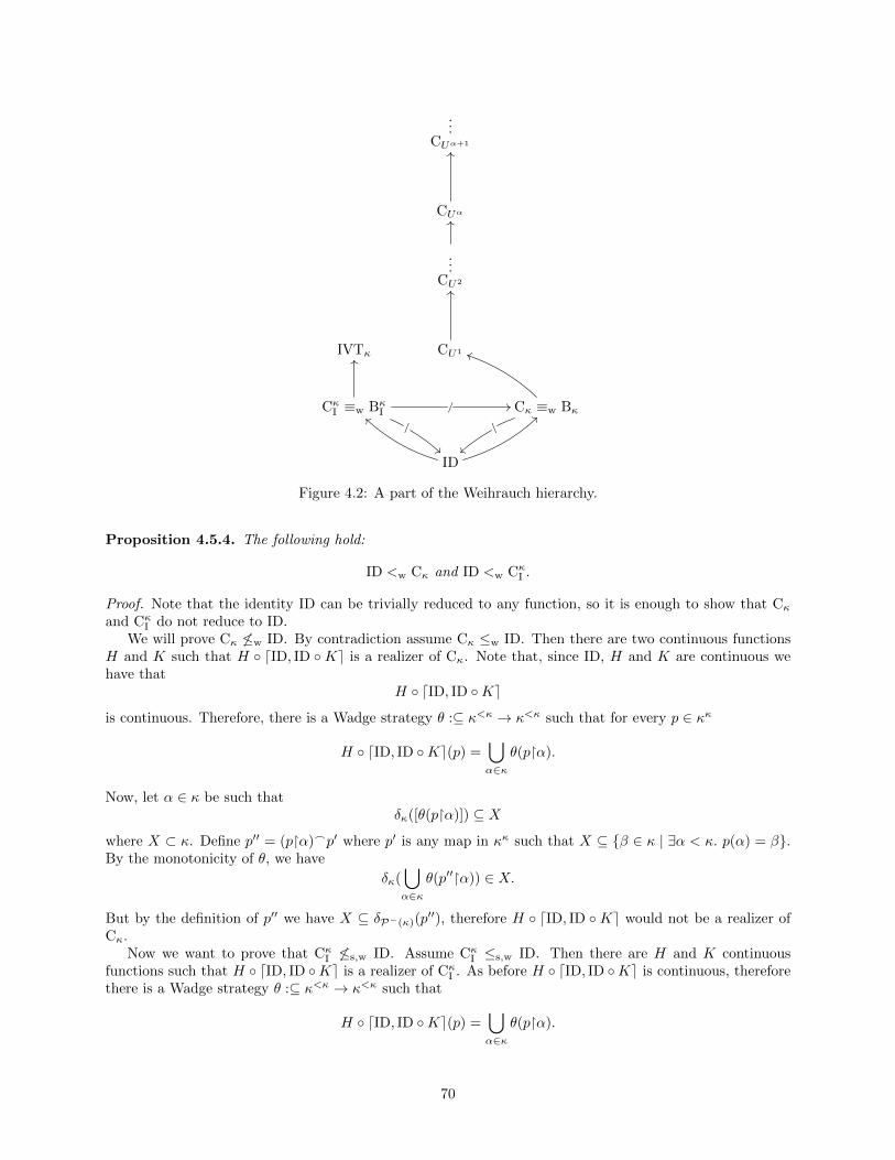
...CUα+1

CUα

OO

...CU2

OO

IVTκ CU1

OO

CκI ≡w BκI

OO

/

/ // Cκ ≡w Bκ

jj

\

~~

ID

`` >>

Figure 4.2: A part of the Weihrauch hierarchy.

Proposition 4.5.4. The following hold:

ID <w Cκ and ID <w CκI .

Proof. Note that the identity ID can be trivially reduced to any function, so it is enough to show that Cκand CκI do not reduce to ID.

We will prove Cκ 6≤w ID. By contradiction assume Cκ ≤w ID. Then there are two continuous functionsH and K such that H ◦ dID, ID ◦Ke is a realizer of Cκ. Note that, since ID, H and K are continuous wehave that

H ◦ dID, ID ◦Ke

is continuous. Therefore, there is a Wadge strategy θ :⊆ κ<κ → κ<κ such that for every p ∈ κκ

H ◦ dID, ID ◦Ke(p) =⋃α∈κ

θ(p�α).

Now, let α ∈ κ be such thatδκ([θ(p�α)]) ⊆ X

where X ⊂ κ. Define p′′ = (p�α)_p′ where p′ is any map in κκ such that X ⊆ {β ∈ κ | ∃α < κ. p(α) = β}.By the monotonicity of θ, we have

δκ(⋃α∈κ

θ(p′′�α)) ∈ X.

But by the definition of p′′ we have X ⊆ δP−(κ)(p′′), therefore H ◦ dID, ID ◦Ke would not be a realizer of

Cκ.Now we want to prove that CκI 6≤s,w ID. Assume CκI ≤s,w ID. Then there are H and K continuous

functions such that H ◦ dID, ID ◦Ke is a realizer of CκI . As before H ◦ dID, ID ◦Ke is continuous, thereforethere is a Wadge strategy θ :⊆ κ<κ → κ<κ such that

H ◦ dID, ID ◦Ke(p) =⋃α∈κ

θ(p�α).

70

Now define the following sequencep = Jι(wα)_ι(w′α)Kα∈κ,

where wα and w′α are such that

I′(wα) = (1

α,

1

2− 1

α) and I′(w′α) = (

1

3+

1

α, 1− 1

α).

Note that δ[0,1](p) = [12 ,23 ] ∪ {0, 1}. Then we have:

δRκ(H ◦ dID, ID ◦Ke(p)) ∈ [1

2,

2

3] ∪ {0, 1}.

Without loss of generality we can assume

δRκ(H ◦ dID, ID ◦Ke(p)) ∈ [1

2,

2

3]

the other cases can be proved similarly. Let α be such that

δRκ([θ(p�α)]) ⊆ [1

2,

2

3].

Now, definep′ = Jι(wα)Kα∈κ,

where wα are such that I(wα) = ( 1α , 1] (note that they are open intervals in [0, 1]). Let p′′ = (p�α)_p′.

Then trivially δ[0,1](p′′) = {0}. But by monotonicity of θ and by the fact that p�α = p′′�α, it follows that

δRκ([θ(p′′�α)]) ∈ [ 12 ,23 ] and then

H ◦ dID, ID ◦Ke(p′′) ∈ [1

2,

2

3].

But this means that H ◦ dID, ID ◦Ke is not a realizer of CκI .

One important tool for studying the Weihrauch degrees of choice principles are the boundedness principles.In particular, reductions with boundedness principles usually result to be easier to construct and will thensimplify our proofs.

Definition 4.5.5 (Boundedness Principles). We define the following boundedness principles:

• BκI : given two Cauchy sequences, (qα)α∈κ and (q′α)α∈κ in Qκ such that

supα∈κ

qα ≤ infα∈κ

q′α,

there is x ∈ Rκ such thatsup qα ≤ x ≤ inf q′α.

Formally we define BκI as follows:

BκI :⊆ R<κ ×R>κ ⇒ Rκ , (x, y) 7→ [x, y] dom(BI) = {(x, y) | x ≤ y}.

• Bκ: given a Cauchy sequence (qα)α∈κ of κ-rationals such that

supα∈κ

qα ≤ r for some r ∈ Rκ.

Intuitively, Bκ chooses a κ-real which is greater than or equal to supα∈κ qα. Formally:

Bκ : R<κ ⇒ Rκ, x 7→ [x,+∞).

71

Now we will focus on proving that as in the classical case we have

Bκ ≡w Cκ and CκI ≡s,w BκI .

The formal proofs of these facts can be slightly convoluted. For this reason, before we prove these resultswe will give an informal intuition of the reason why they work.

First we will prove that Bκ ≡w Cκ. While it is not complicated to prove that Bκ ≤w Cκ, the proof forthe other direction is less intuitive.

We are given an enumeration of a set A ⊂ κ and we want to find an element in κ \A by using a realizerof Bκ. To find this element, we read the enumeration of A and we build two sequences of rational numbershp and fp. The sequence hp will keep track of the smallest ordinal number not in the portion of A we haveread so far. The sequence fp, instead, will be a strictly Cauchy sequence whose limit is the position in whichhp becomes constant. Intuitively hp is defined as follows:

Start by setting hp(0). Then look at a0, namely the first element of the enumeration of A. If a0 > 0 thenhp(1) = a0 otherwise hp(1) = hp(0). In general for aα we have hp(α) = aα if aα > hp(β) for every β < α,and hp(α) =

⋃β∈α hp(β) otherwise.

By using this sequence we can define fp. Intuitively fp will guess the smallest position on which hpstabilizes.

We start defining fp(0) = − 12 , guessing that the hp is the constant 0. Now we check hp(1), if it is 0, then

our guess is sill valid and we set fp(1) = − 13 . Otherwise we guess that hp stabilizes at position 1 and set

fp(1) = 13 . In general, we check hp(α), if this does not contradict our guess g we keep defining a sequence

converging at g by setting fp(α) = g− 1α+1 , otherwise we change our guess to α and we set fp(α) = α− 1

α+1 .Note that since κ \ A is nonempty, then fp is Cauchy. Now we can feed a realizer of Bκ with hp and it

will find an upper bound r of fp. The κ-real r will be given to us as a fast converging Cauchy sequence.Therefore we can easily find an ordinal αm which is bigger than r. Now we can go through the enumerationof A again and find the least upper bound of the first αm elements of A. This number will be by definitionin κ \A as desired.

Proposition 4.5.6. Bκ ≡w Cκ.

Proof. First we will prove Cκ ≤w Bκ. Let p be an enumeration of the set A. We want to find an elementnot in A. We define the following sequence:

hp(0) = 0,

hp(α) = minκ \ {p(β) | β ≤ α}.

Intuitively hp(α) is the minimum ordinal which is not in A according to the information in p�(α+ 1). Nowby using hp we can define the following sequence:

sp(0) = 0,

sp(α+ 1) =

{sp(α) If hp(α) = hp(α+ 1),

α+ 1 otherwise,

sp(λ) =⋃α∈λ

sp(α).

The intuition is that sp keeps track of the changes in hp. Since A is non empty, sp is increasing and eventuallyconstant, hence Cauchy. In particular sp is a Cauchy sequence whose limit ` is an index of p such that hp(`)is the smallest ordinal not in A. We want to extract form sp a strictly increasing subsequence. We define:

fp(α) = sp(α)− 1

α+ 1.

The Cauchy sequence fp is trivially increasing and has limit `. Therefore we can define K as follows:

K(p) = Jι(ν−1Qκ (fp(α)))Kα∈κ.

72

Note that, for every α, we use only a small portion of p in order to define fp(α), therefore K is continuous.Note that Bκ(K(p)) is a κ-real number greater than every element in A. It is not hard to see that, since

Bκ(K(p)) is fast convergent, by considering an initial portion of Bκ(K(p)) of length less than κ we can findan ordinal αm which is not in A (note that is enough to pick αm such that αm > Bκ(K(p))). Then we candefine the function H as follows:

H(dp,Bκ(K(p))e) = minκ \ {p(α) | α < αm}_0,

where 0 is the constant 0 sequence in κκ. Now, note that H is continuous and δκ(H(dp,Bκ(K(p))e)) ∈ κ \Aas desired.

Now we want to show that Bκ ≤s,w Cκ. Let p be the code of a strictly increasing Cauchy sequence(qα)α∈κ of κ-rationals. We want to find a κ-real which is greater than or equal to the least upper bound ofthe sequence. Define K as follows:

K(p)(dα, βe) =

β If p�α codes the sequence (qγ)γ∈γ′,

and there exists γ ≤ γ′ such that β ≤ qγ ,γ0 otherwise,

where γ0 is the smallest ordinal such that γ0 ≤ q0. Since for defining an initial segment of K(p) we onlyneed a small portion of p, we have that K is continuous. Now define H(α) = α_0. We claim that K(p)is a code for the set of all the ordinal numbers smaller than or equal to ` = limα∈κ qα. Indeed, if β ≤ `there is qα such that β ≤ qα. Take γ be such that p�γ codes the sequence (q′γ)γ′∈γ′′ with α ≤ γ′′. ThereforeK(p)(dγ, βe) = β. On the other hand, if K(p)(dα, βe) = γ, either γ = γ0 ≤ q0 or there is an element qγ′ ofthe sequence coded by p such that γ ≤ qγ′ .

Now by using Cκ, we obtain an ordinal which is greater than or equal to `. Then we can define a continuousfunction H(p) = p′, where p′ is any code for p(0) in Rκ. Therefore we have δRκ(H ◦Cκ ◦K(p)) ∈ [`,+∞) asdesired.

We will now prove that CκI ≡s,w BκI . Let us illustrate the idea behind the proof of CκI ≤s,w BκI . We aregiven a closed subinterval [r, r′] of [0, 1] as the listing of all the open intervals with κ-rational end pointswhich have empty intersection with it. We have to define two sequences (qα)α∈κ and (q′α)α∈κ of κ-rationals,respectively strictly increasing and strictly decreasing such that every element x in between supα∈κ qα andinfα∈κ q

′α is in [r, r′]. Let us consider the construction of (qα)α∈κ, a similar reasoning works for (q′α)α∈κ. The

idea is that of building a Cauchy sequence for r. We can start by setting q0 = 0. Now we start reading thedescription of [r, r′] until we find enough open intervals to cover [0, q] with q any κ-rational. Then we aresure that q < r and we can set q1 = q. In general to define qα we read an initial portion of the code of [r, r′]long enough to cover [0, q] with q strictly bigger than all the qβ for β < α and we set qα = q. It is not hardto see that this is a strictly increasing Cauchy sequence converging to r as we wanted.

Proposition 4.5.7. CκI ≡s,w BκI .

Proof. First we prove CκI ≤s,w BκI . Let p code the closed interval [r, r′] ⊂ [0, 1]. In particular assumethat p is the listing of open intervals (Jα)α∈κ such that

⋃α∈κ Jα = Rκ \[r, r′]. We want to define two

Cauchy sequences (qα)α∈κ and (q′α)α∈κ in Rκ respectively strictly increasing and strictly decreasing, suchthat supα∈κ qα ≤ infα∈κ q

′α. Let (q′′α)α∈κ be a listing of Qκ. We define

q0 = 0, q′0 = 1,

qα = q′′mwhere m = min{β | [0, q′′β ] ⊆⋃γ∈αm

Jγ ∧ q′′β > {qγ | γ < α}},

q′α = q′′mwhere m = min{β | [q′′β , 1] ⊆⋃γ∈α′m

Jγ ∧ q′′β < {q′γ | γ < α}},

where αm and α′m are the smallest ordinals such that

{β | [0, q′′β ] ⊆⋃γ∈αm

Jγ ∧ q′′β > {qγ | γ < α}} 6= ∅

73

and{β | [q′′β , 1] ⊆

⋃γ∈α′m

Jγ ∧ q′′β < {q′γ | γ < α}} 6= ∅.

Note that αm and α′m exist by definition of (Jα)α∈κ and by the fact that the κ-rationals are dense inRκ. Hence the sequences are well defined. Moreover, by definition, (qα)α∈κ and (q′α)α∈κ are Cauchy andrespectively strictly increasing and decreasing. We claim supα∈κ qα = r and infα∈κ q

′α = r′. Since every qα

is in some Jγ , it follows that r is an upper bound of (qα)α<κ. Moreover let r′′ < r be such that r′′ is anupper bound of (qα)α<κ. Then there is a rational r′′ < q′′γ′ < r, and q′′γ′ ∈ Jγ for some γ < κ. Then forα > γ there is qα = q′′γ′′ with γ′′ > γ′. But since q′′γ′ > r′′ ≤ (qα)α∈κ and [0, q′′γ′ ] ⊂

⋃β<αm

Jβ , it followsthat qα = q′′γ′′ implies γ′′ ≤ γ′ which contradicts our assumption. A similar proof shows infα∈κ q

′α = r′.

Then the function K : p 7→ dp′, p′′e where p′ and p′′ are respectively Jι(ν−1Qκ (qα))Kα∈κ and Jι(ν−1Qκ (q′α))Kα∈κ is

continuous. Moreover, taking bκI any realizer of BκI we have δRκ(bκIK(p)) ∈ [r, r′] as desired.Now we want to prove BκI ≤s,w CκI . First of all note that the function f : (0, 1)→ Rκ defined as

f(x) =2x− 1

x− x2

is a homeomorphism between (0, 1) and Rκ. Indeed, since f is definable in the language of real closed fieldsand it is a strictly increasing bijection over R it is a strictly increasing bijection over Rκ. Moreover, since(r, r′) ∈ Rκ, we have f((r, r′)) = (2r−1

r−r2 ,2r′−1r′−r′2 ), it follows that f is open in Rκ.

Now let p be the code of the two Cauchy sequences (qα)α∈κ and (q′α)α∈κ, respectively strictly increasingand strictly decreasing. Define the following sequence:

p′ = dJI ′−1([0, f(qα))Kα∈κ, JI ′−1((f(q′α), 1])Kα∈κe.

Since to define a small prefix of p′ only a small prefix of p is needed, the function K : p 7→ p′ is continuous.Now by the fact that f−1 is continuous in Rκ it has a continuous realizer F−1. Define H = F−1. Then,given cκI a realizer of CκI , we have that cκIK(p) is the code for a real number in [f(supα∈κ qα), f(infα∈κ q

′α)]

and then δRκ(HcκIK(p)) ∈ [supα∈κ qα, infα∈κ q′α] as desired.

Now we define the following set:

U1 =⋃α<κ

{p ∈ κκ | p(α) 6= 0}.

We end this section by showing that CU1 is strictly more complex than Cκ.

Proposition 4.5.8. Cκ ≤s,w CU1 .

Proof. Define K as follows:

K(p)(dα, βe) =

{1 if ∃γ < α. p(γ) = β,

0 otherwise,

therefore K is continuous. Moreover let H be defined as follows:

H(p) = β_0 iff β < κ is the least such that p(β) = 0,

where 0 is the constant 0 function in κκ. Note that H is trivially continuous in its domain. Then for everyrealizer cU1 of CU1 and p ∈ dom(CU1) such that p codes the complement of A ⊂ κκ, we have:

(H ◦ cU1 ◦K)(p) = β ⇔ cU1K(p)(β) = 0

⇔ ∀α < κ. K(p)(dα, βe) = 0

⇔ ∀γ < κ. p(γ) 6= β

⇔ β /∈ A,

therefore Cκ ≤s,w CU1 as desired.

74

Now we want to prove that CκI and Cκ characterize two different Weihrauch degrees. By following Brattkaand Gherardi we can prove that CκI does not reduce to Cκ (the interested reader is referred to [5, Proposition4.9]). The only difference between our proof and the classical proof is in the use of the κ-Baire CategoryTheorem. While in the standard proof the BCT could be used without any problem, in this case we needto show that all the requirements of the BCTκ we presented in Section 3.5 are fulfilled by the space we areworking with.

Proposition 4.5.9. CκI 6≤w Cκ.

Proof. By Propositions 4.5.7 and 4.5.6, it is enough to prove BκI 6≤w Bκ. We define δ = δR<κ ⊗ δR>κ . Bycontradiction assume BκI ≤w Bκ. Then there are two continuous functions H and K such that for everyrealizer bκ of Bκ we have that

H ◦ dID, bκ ◦Ke is a realizer of BκI .

Consider the following closed set

C = {dp, qe ∈ κκ | δR<κ (p) ≤ δR>κ (q)}.

Without loss of generality we can assume dom(K) = C. Then define the following sequence:

Pα = {p ∈ κκ | δR<κ (K(p)) ≤ α},

for α ∈ κ. Note that, since K is continuous, we have that for every α ∈ κ the set Pα is closed in dom(K).Moreover, since C is closed and κκ is κ-Polish, C is completely κ-metrizable. We claim that C satisfies therequirement of the κ-Baire Category theorem (see Theorem 3.5.25). As we have just seen, C =

⋃α∈κ Pα.

Moreover by the definition for every α < β < κ, we have Pα ⊆ Pβ . Now let {Iα}α∈γ with γ < κ be a familyof nested open balls such that for every α < γ, we have C ∩ Iα 6= ∅. We want to prove that C ∩

⋂α∈γ Iα 6= ∅.

Then we have∀α < γ∃ηα < κ. Pηα ∩ Iα 6= ∅

and by regularity of κ, we have∃η < κ∀α. ηα < η.

Moreover, by monotonicity of (Pα)α∈κ∀α < γ. Pηα ⊆ Pη,

therefore∀α < γ. Iα ∩ Pη 6= ∅,

which by Corollary 3.5.25 implies ⋂α∈γ

Iα ∩ Pη 6= ∅.

In conclusion⋂α∈γ Iα ∩ C = C ∩

⋂α∈γ Iα 6= ∅ as desired.

By the κ-Baire Category Theorem (i.e., Theorem 3.5.24), we have that there are α ∈ κ and w ∈ κ<κsuch that ∅ 6= [w] ∩ C ⊂ Pα. Now we fix a realizer bκ of Bκ defined as follows

δκ(bκ(p)) = max{α,min{β | β ≥ δR<κ (p)}}.

Then we havePα = {p ∈ κκ | δκ(bκ(K(p))) = α}.

Without loss of generality we can assume that w is long enough to code the interval [a, b] (i.e., δ([w]) ⊂ [a, b]).Now take p ∈ κκ such that w ⊂ p and I = BκI δ(p) = [a′, b′] with a < a′ < b′ < b. Then by definitionx = δRκ(H(dp,BκK(p)e)) ∈ I. This means that either x ∈ [a′, b′) or x ∈ (a′, b′]. Assume that x ∈ (a′, b′], asimilar proof works for the other case. Take an open interval J such that a′ < J . By continuity of δRκ ◦H,there is v ∈ κ<κ such that w ⊂ v ⊂ p and δRκ(Hd[v],BκH(p)e) ⊂ J . As before assume v long enough torepresent an interval [a′′, b′′] such that

a < a′′ < a′ < b′ < b′′ < b.

75

Then there is p′ ∈ κκ such that BκI δ(p′) ⊆ (a′′, a′]. Hence

δRκ(H(dp′, bκK(p′)e)) /∈ J.

But since p′ ∈ [w] we have δRκ(H(dp′, bκK(p)e)) ∈ J and bκK(p) = bκK(p′). This contradicts the hypothesis.Therefore H and K do not reduce BκI to Bκ.

In Figure 4.2 many arrows are still missing. In particular we have:

Open Question 4.5.10. Are the following true:

Q1: Cκ 6≤w CκI .

Q2: CκI ≤w CU1 .

Note that that a positive answer to Q1 would imply CU1 6≤w Cκ and a positive answer to Q2 wouldimply CU1 6≤w CκI . Moreover, note that in the literature there are no direct proofs for the classical versionfor Q1 and Q2. Indeed, Q1 is usually proved by using omniscience principles and parallelization, while Q2 isproved by showing that CI <w CK <w CA, where CI, CK and CA are closed intervals, closed sets and densesets choice, respectively. A generalization of these notions is needed to start the study of Q1 and Q2 (for anoverview on the classical approaches see [5]).

4.6 Baire Choice Functions

In this section we will start the study of the choice functions CU for a particular class of sets U whichcharacterize the Borel measurable functions over the generalized Borel hierarchy. These choice functions arethe generalization of those introduced by Brattka in [3].

Let us fix for every λ < κ+ limit a surjective function fλ : κ→ λ. Define the following sets:

U1 =⋃α∈κ{p ∈ κκ | p(α) 6= 0},

Uα+1 = {p ∈ κκ | ∃β < κ. (p)β 6∈ Uβ},Uλ = {p ∈ κκ | ∃α < κ. (p)α 6∈ Ufλ(α)}.

First of all let us generalize the definition of Wadge reducibility from classical descriptive set theory.

Definition 4.6.1 (Wadge Reducibility). Let U and V be two subsets of κκ. Then U is said to be Wadgereducible to V , in symbols U ≤wa V iff there is a continuous function f :⊆ κκ → κκ such that

x ∈ U ⇔ f(x) ∈ V.

As usual, if U ≤wa V and V ≤wa U we will say that U is Wadge equivalent to V , in symbols V ≡wa U .Moreover, let A ⊂ P−(κκ). If U ∈ A and for every V ∈ A we have that V ≤wa U , then U is said to beWadge complete with respect to A.

Now we want to prove that for every α < κ+, the set Uα is Wadge complete w.r.t. the κ-Borel class

Σ(κ,0)α (κκ). First note that the κ-Borel classes are closed under Wadge reducibility:

Proposition 4.6.2. For every α < κ+, the sets Σ(κ,0)α (κκ) and Π

(κ,0)α (κκ) are closed under Wadge reduction.

Proof. We will proceed by induction over α.

Let α = 1. Assume U ∈ Σ(κ,0)1 (κκ) and let V ⊂ κκ be such that V ≤wa U . Then there is a continuous

f such that f−1[U ] = V . Now since by definition U is open in κκ and f is continuous, V is open in κκ.

Therefore V ∈ Σ(κ,0)1 (κκ) as desired. A similar proof works for Π

(κ,0)α (κκ).

Now let α > 1. Assume U ∈ Σ(κ,0)α (κκ), then there are (Uβ)β∈κ and (ηβ)β∈κ such that U =

⋃β<κ Uβ and

for every β < κ we have ηβ < α and Uβ ∈ Π(κ,0)ηβ (κκ). Moreover assume V ⊂ κκ and f continuous such that

V ≤wa U . By inductive hypothesis we have f−1[Uβ ] ∈ Π(κ,0)ηβ (κκ) for every β ∈ κ. Then V =

⋃β∈κ g

−1[Uβ ]

and V ∈ Σ(κ,0)α (κκ) as desired.

76

Note that by the previous proposition and by the fact that the κ-Borel hierarchy over κκ does not collapse,we have the following:

Corollary 4.6.3. If U is Wadge complete for Σ(κ,0)α (κκ), V is Wadge complete for Σ

(κ,0)β (κκ) and α < β,

then V 6≤wa U .

Proof. Assume V ≤wa U . Then Σ(κ,0)α (κκ) = Σ

(κ,0)β (κκ). By Theorem 3.5.18 this is a contradiction.

Now we will prove that for every α, the set Uα is Wadge complete for Σ(κ,0)α (κκ).

Theorem 4.6.4. Let α < κ+. Then Uα is Wadge complete for Σ(κ,0)α (κκ).

Proof. We proceed by induction over α.For α = 1, we have:

U1 =⋃γ∈κ{p ∈ κκ | p(γ) 6= 0}.

Note that U1 is trivially open. Therefore U1 ∈ Σ(κ,0)1 (κκ). Moreover, let V ∈ Σ

(κ,0)1 (κκ). Since V is open

there is a sequence (wγ)γ∈κ in κ<κ such that V =⋃γ∈κ[wγ ]. Define the following function:

g(p)(α) =

{1 If ∃γ < κ. wγ = p�α,

0 otherwise.

Then g is continuous. Moreover we have

g−1[U1] =⋃β∈κ

{p ∈ κκ | g(p)(β) 6= 0}

=⋃β∈κ

{p ∈ κκ | ∃γ < κ. p�β = wγ}

=⋃β∈κ

⋃γ∈κ{p ∈ κκ | p�β = wγ}

=⋃γ∈κ

[wγ ] = V

as desired.For α = β + 1, we have

Uβ+1 = {p ∈ κκ | ∃γ < κ. (p)γ 6∈ Uβ}.

By inductive hypothesis Uβ ∈ Σ(κ,0)β (κκ). Moreover by definition

Uα =⋃γ∈κ{p ∈ κκ | (p)γ /∈ Uβ},

therefore Uα ∈ Σ(κ,0)α (κκ). Now let V ∈ Σ

(κ,0)α (κκ). Then there are (Vγ)γ∈κ such that Vγ ∈ Π

(κ,0)β (κκ) for

every γ ∈ κ and V =⋃γ∈κ Vγ . Moreover, since Uβ is Wadge complete for Σ

(κ,0)β (κκ), there are continuous

functions (fγ)γ∈κ such that f−1γ [(κκ \ Uβ)] = Vγ for every γ ∈ κ. Now define a continuous function f asfollows:

(f(p))γ = fγ(p) ∀p ∈ κκ∀γ ∈ κ.We have that

p ∈ V ⇔ ∃γ < κ.p ∈ Vγ⇔ ∃γ < κ.(f(p))γ = fγ(p) /∈ Uβ

⇔ f(p) ∈ Uα

77

as desired.Finally if α = λ limit. By definition we have

Uλ = {p ∈ κκ | ∃γ < κ. (p)γ 6∈ Ufλ(γ)}.

First note thatUλ =

⋃γ∈κ{p ∈ κκ | (p)γ /∈ Ufλ(γ)}.

Moreover, by inductive hypothesis we have

{p ∈ κκ | (p)γ /∈ Ufλ(γ)} ∈ Π(κ,0)fλ(γ)

(κκ)

and therefore Uλ ∈ Σ(κ,0)λ (κκ). Now let V ∈ Σ

(κ,0)λ (κκ). By definition there are (Vγ)γ∈κ with Vγ ∈ Π

(κ,0)ηγ (κκ)

and ηγ < λ for every γ < λ, such that V =⋃γ∈κ Vγ . Define the sequence (V ′α)α∈κ as follows:

V ′β =

{Vβ iff ηβ ≤ fλ(β),

∅ otherwise.

Then V =⋃γ∈κ V

′γ and for all γ < κ we have V ′γ ∈ Π

(κ,0)fλ(γ)

(κκ). Hence by inductive hypothesis there are

(fγ)γ∈κ continuous such that f−1γ [(κκ \ Ufλ(γ)] = V ′γ for every γ ∈ κ. Define a continuous function f asfollows:

(f(p))γ = fγ(p).

Hence we have

p ∈ V ⇔ ∃γ < κ.p ∈ V ′γ⇔ ∃γ < κ.(f(p))γ = fγ(p) /∈ Ufλ(γ)

⇔ f(p) ∈ Uλ

as desired.

Now we want to use the fact that for all α, the set Uα is Wadge complete for Σ(κ,0)α (κκ) in order to

prove that every CUα characterize set of Σ(κ,0)α+1 (κκ)-measurable functions w.r.t. Weihrauch reductions. First

we extend the definitions we need from descriptive set theory and from computable analysis to generalizedBaire space.

Definition 4.6.5 (Weihrauch Completeness). A function f :⊆ κκ → κκ is Weihrauch complete with respectto the set A ⊂ (κκ)κ

κ

iff f ∈ A and for every g ∈ A, g ≤w f .

Definition 4.6.6. A function f :⊆ κκ → κκ is Σ(κ,0)α (κκ)-measurable iff f−1[O] ∈ Σ

(κ,0)α (κκ) for every

open set O in κκ. We will denote the set of Σ(κ,0)α (κκ)-measurable functions with Mα.

Note that the sequence of (Mα)α<κ+ is increasing.

Theorem 4.6.7. The function CUα is Weihrauch complete for Mα+1.

Proof. First of all to prove that CUα is in Mα+1, let w ∈ κ<κ. We have:

C−1Uα [w] = {p ∈ κκ | CUα(p) ∈ [w]}= {p ∈ κκ | ∀β < |w|. (p)β ∈ Uα ⇔ w(β) = 0}

=⋂

β<|w|w(β)=0

{p ∈ κκ | (p)α ∈ Uα} ∩⋂

β<|w|w(β)=1

{p ∈ κκ | (p)α 6∈ Uα}.

78

Since in κκ intersections of less than κ open set are open, we have C−1Uα [w] ∈ Σ(κ,0)α+1 (κκ) as desired.

Now we want to show that CUα is Weihrauch complete for Mα+1. Let f :⊆ κκ → κκ be a function in

Mα+1. Fix a bijection b : κ→ κ<κ. Since f is in Mα+1, there is a sequence (Vγ)γ∈κ of elements of Σ(κ,0)α (κκ),

such thatf−1[b(γ)] =

⋃β∈Iγ

(κκ \ Vβ),

for some sequence (Iγ)γ∈κ with Iγ ⊂ κ for every γ < κ. Since we know that Uα is Wadge complete for

Σ(κ,0)α (κκ), for each γ < κ, there is gγ :⊆ κκ → κκ continuous such that

f−1[b(γ)] =⋃β∈Iγ

(κκ \ g−1β [Uα]).

Now define the continuous function K :⊆ κκ → κκ as follows:

(K(p))γ = gγ(p),

for every γ ∈ κ and p ∈ κκ. Then we have

f(p) ∈ [b(γ)]⇔ p ∈ f−1[b(γ)]

⇔ ∃β ∈ Iγ . p ∈ (κκ \ g−1β [Uα])

⇔ ∃β ∈ Iγ . gβ(p) /∈ Uα

⇔ ∃β ∈ Iγ . (K(p))β /∈ Uα

⇔ ∃β ∈ Iγ . CUα(K(p))(β) = 1.

Now define H :⊆ κκ → κκ as follow:

H(p) =⋃{b(γ) | ∃β ∈ Iγ . p(β) = 1}.

Therefore H and K are continuous in their domains. Moreover we have

H(CUα(K(p))) =⋃{b(γ) | ∃β ∈ Iγ . CUα(K(p)) = 1}

=⋃{b(γ) | f(p) ∈ [b(γ)]}

= f(x).

Hence H and K reduce f to CUα as desired.

From the previous theorem we have:

Corollary 4.6.8. For every 1 ≤ α, β < κ+, if α ≤ β, then CUα ≤w CUβ .

Note that, since we are not guaranteed that the sequence (Mα)α∈κ+ does not collapse, we do not knowif the sequence (CUα)α∈κ+ collapses. In particular we leave the following open question:

Open Question 4.6.9. Is it true that for every 1 ≤ α, β < κ+ such that α < κ, we have CUβ 6≤w CUα?

4.7 Representation of the IVT

In this last section we will start the study of the IVTκ by means of Weihrauch degrees.First of all note that the IVTκ can be stated as follows:

∀f ∈ C[a,b]∃c ∈ [a, b]. f(c) = 0,

79

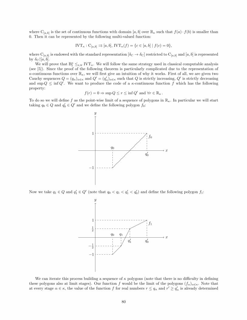
where C[a,b] is the set of continuous functions with domain [a, b] over Rκ such that f(a) · f(b) is smaller than0. Then it can be represented by the following multi-valued function:

IVTκ : C[a,b] ⇒ [a, b], IVTκ(f) = {c ∈ [a, b] | f(c) = 0},

where C[a,b] is endowed with the standard representation [δC → δC] restricted to C[a,b] and [a, b] is representedby δC�[a, b].

We will prove that BκI ≤s,w IVTκ. We will follow the same strategy used in classical computable analysis(see [5]). Since the proof of the following theorem is particularly complicated due to the representation ofκ-continuous functions over Rκ, we will first give an intuition of why it works. First of all, we are given twoCauchy sequences Q = (qα)α∈κ and Q′ = (q′α)α∈κ such that Q is strictly increasing, Q′ is strictly decreasingand supQ ≤ inf Q′. We want to produce the code of a κ-continuous function f which has the followingproperty:

f(r) = 0⇒ supQ ≤ r ≤ inf Q′ and ∀r ∈ Rκ .

To do so we will define f as the point-wise limit of a sequence of polygons in Rκ. In particular we will starttaking q0 ∈ Q and q′0 ∈ Q′ and we define the following polygon f0:

x

y

q0

q′0

−1

1f0

Now we take q1 ∈ Q and q′1 ∈ Q′ (note that q0 < q1 < q′1 < q′0) and define the following polygon f1:

x

y

q0

q′0q′1

q1

−1

1

12

− 12

f1

We can iterate this process building a sequence of κ polygons (note that there is no difficulty in definingthese polygons also at limit stages). Our function f would be the limit of the polygons (fα)α∈κ. Note thatat every stage α ∈ κ, the value of the function f for real numbers r ≤ qα and r′ ≥ q′α is already determined

80

by its value on fα. We can then use this fact to build a continuous function that given a code for Q andQ′ returns a code for f . In particular if we start reading Q and Q′ at some point we read the first α < κelements of both the sequences. Then we will have enough information to determine the values of f for allthose κ-reals which are either smaller than qα or greater than q′α. Following the intuition given by Wadgestrategies, the process we have just described defines a continuous reduction of BκI to IVTκ.

Theorem 4.7.1. BκI ≤s,w IVTκ.

Proof. Let (qα)α∈κ and (q′α)α∈κ be two sequences of rational numbers such that supα∈κ qα ≤ infα∈κ q′α. Note

that by the definition of BκI , the sequence (qα)α∈κ is strictly increasing and the sequence (q′α)i∈κ is strictlydecreasing. We want to define a κ-continuous function f such that for every x ∈ Rκ, if f(x) = 0, thenx ∈ [supα∈κ qα, infα∈κ q

′α]. We define a sequence of functions (fα)α∈κ such that limα∈κ fα = f as follows:

f0(x) =2

q′0 − q0(x− q0)− 1,

fα+1(x) =

fα(x) iff x ≤ qα ∨ x ≥ q′α,

1(α2+α)(qα+1−qα) (x− qα)− 1

α iff qα < x < qα+1,1

(α2+α)(q′α−q′α+1)(x− q′α+1) + 1

α+1 iff q′α+1 < x < q′α,

2(α+1)(q′α+1−qα+1)

(x− qα+1)− 1α+1 otherwise

fλ(x) =

fβ(x) iff ∃β < λ. qβ ≤ x ≤ qβ+1,

fβ(x) iff ∃β < λ. q′β+1 ≤ x ≤ q′β ,2

λ(q′λ−qλ)(x− qλ)− 1

λ otherwise.

Note that for every x if x ∈ (qα, qα+1) or x ∈ (q′α+1, q′α) for some α < k then for all β ≥ α we have

fβ(x) = fα(x). Hence (fα)α∈κ is well defined. By an easy induction one can prove the following properties:

If x ∈ [qβ , qβ+1] for some β < α then − 1

β< fα(x) < − 1

β + 1.

If x ∈ [q′β+1, q′β ] for some β < α then

1

β + 1< fα(x) <

1

β.

If x ∈ (qα, q′α) then − 1

α< fα(x) <

1

α.

Now let α ∈ κ. We claim that for every x ∈ Rκ and β, γ > 2α the following holds:

|fβ(x)− fγ(x)| < 1

α.

Without loss of generality assume β < γ. We have the following cases:If x ∈ [qβ′ , qβ′+1] or x ∈ [q′β′+1, q

′β′ ] for some β′ < β, then

|fβ(x)− fγ(x)| = 0 <1

α.

If x ∈ (qγ , q′γ), then we have

− 1

γ< fγ(x) <

1

γand − 1

β< fβ(x) <

1

β.

Now, since 2α < β < γ we have

|fβ(x)− fγ(x)| ≤ 2

γ<

1

α

as desired.

81

If x ∈ [qγ′ , qγ′+1] for β < γ′ < γ, then we have that

− 1

β< fβ(x) <

1

β

and

− 1

γ′< fγ(x) < − 1

γ′ + 1,

therefore

|fβ(x)− fγ(x)| ≤ 2

γ<

1

α

as desired.Hence for every x, (fα(x))α∈κ is a Cauchy sequence and f(x) = limα∈κ fα(x) is well defined over Rκ.Moreover we claim that f�[q0, supα∈κ qα] and f�[infα∈κ q

′α, q′0] are strictly increasing. First we prove that

for every α < κ, the polygon fα is strictly increasing. By induction over α:Assume α = 0. Note that f0 is trivially strictly increasing.Assume α = α′ + 1. Take x, y ∈ [q0, q

′0] with x < y. We only prove some cases (the others are proved

similarly):

• if x, y ≤ qα′ or x, y ≥ q′α′ or x ≤ qα′ and y ≥ qα′ , then the statement follows by inductive hypothesis.

• if x, y ∈ (qα′ , qα), we have

1

(α′ · α′ + α)(qα′+1 − qα′)(x− qα′)−

1

α′<

1

(α′ · α′ + α)(qα′+1 − qα′)(y − qα′)−

1

α′

iff x < y.

• if x ∈ (qα′ , qα) and y ∈ (q′α, q′α′) the statement follows form the fact that

− 1

α′< fα(x) < − 1

α

and1

α′< fα(y) <

1

α.

For α = λ limit, the proof is analogous to that for the successor case.Now we have that f�[q0, supα∈κ qα] and f�[infα∈κ q

′α, q′0] are strictly increasing. Indeed, let x, y ∈

[q0, supα∈κ qα] (a similar argument works for x and y in [infα∈κ q′α, q′0]). Then we have the following cases:

If y = supα∈κ qα then, since limα∈κ1α = 0 and for every β ≤ α

fβ(qα) = − 1

α,

hence we have thatf(supα∈κ

qα) = 0.

Moreover, since x < supα∈κ qα, there is α < κ such that qα ≤ x ≤ qα+1 therefore for every β ≥ α we have

fβ(qα) ≤ fβ(x) ≤ fβ(qα+1) < 0

and for every β ≥ α we have

fβ(qα) = fα(qα),fβ(x) = fα(x), fβ(qα+1) = fα(qα+1).

Hencef(qα) ≤ fβ(x) ≤ f(qα+1) < 0 = f(y).

82

Let α, β ∈ κ such that qα ≤ x ≤ qα+1 and qβ ≤ y ≤ qβ+1. For the same reasons used in the previous casewe have:

fm(x) ≤ fm(qα+1) ≤ fm(qβ) ≤ fm(y),

where m = max{α, β}. Now, since fm is strictly monotonic, one of the inequalities is strict. Moreover, sinceα′ ≥ m we have

fα′(x) = fm(x), fα′(y) = fm(y),

fα′(qα+1) = fm(qα+1), fα′(qβ) = fm(qβ).

Therefore, f(x) < f(y) as desired.Now note that f�[q0, supα∈κ qα] and f�[infα∈κ q

′α, q′0] are also surjective respectively over [−1, 0] and [0, 1].

Hence by Lemma 3.2.5 they are κ-continuous. Moreover f�[supα∈κ qα, infα∈κ q′α] is the constant function 0

hence it is κ-continuous. But then, by Theorem 3.4.24 f is κ-continuous as desired.Finally we will prove that the function reducing BκI to IVTκ is continuous.Let us fix a listing of codes for Cauchy sequences (pr)r∈Rκ such that δC(pr) = r. Let w ∈ κ<κ be such

that it is an initial segment for a code of the sequences (qα)α∈κ and (q′α)α∈κ in Qκ such that supα∈κ qα ≤infα∈κ q

′α. Without loss of generality we can assume that w is long enough to contain the code for two

initial subsequences (qα)α∈γ and (q′α)α∈γ′ respectively of (qα)α∈κ and (q′α)α∈κ. Note that (qα)α∈γ is strictlyincreasing and (q′α)α∈γ′ is strictly decreasing. We define a Wadge strategy θ :⊆ κ<κ → κ<κ as follows:

θ(w) = w′,

where w′ is defined as follows:Let b : κ<κ → κ be the bijection used to define δWs (see Section 4.3). First we want to determine the

length of w′. Let B be the following set:

B = {β′ | ∀α < β′(∃α′ < γ. δC[b−1(α)] ⊂ [qα′ , qα′+1])∨(∃α′′ < γ′.δC[b−1(α)] ⊂ [q′α′′+1, q

′α′′ ])}.

Intuitively B is the set of ordinals β′ such that every α < β′ is the code of a prefix of a real number whichhas already been determined not to be in between supγ∈κ qγ and infγ∈κ q

′γ . The situation is illustrated by

the following figure:

Now, by using B, we can determine the length of w′. Let the length of w′ be the following ordinal:

` =

{maxB If B is bounded,

|w| otherwise.

Then for every α < `, the sequence w′(α) is defined as follows:If δC([b−1(α)]) = ∅: then w′(α) is the prefix of length |w| of p0 (the Cauchy sequence for 0). Note that

these entries are meaningless for [δC → δC].

83

If δC([b−1(α)]) 6= ∅: in this case we know that f(δC([b−1(α)])) is already partially determined. In fact bydefinition of `, we know that δC([b−1(α)]) is going to be in between two of the κ-rationals of the sequenceswe have processed so far. Hence, we have that

δC([b−1(α)]) ⊆ [qα′ , qα′+1] or δC([b−1(α)]) ⊆ [q′α′+1, q′α′ ],

for some α′ < γ. Let αm be the minimal such α′. Then w′(α) is defined as the longest common prefix of thesequences in the following set:

{pr | r ∈ fαm(δC([b−1(α)]))}.

Note that, by the definition of ` and since the κ-rational sequences are monotone, then θ is monotone.Let h′ : κκ → κκ be the continuous function:

h′(p) =⋃α∈κ

(θ(p�α)),

where dom(h) is the set of codes of sequences of κ-rationals (qα)α∈κ and (q′α)α∈κ. Then for every p ∈ dom(h′)and p′ ∈ κκ, we have

f(δC(p′)) = δC(⋃α∈κ

h′(p)(p′�α))

and therefore [δC → δC](h′(p)) = f as desired.

In the classical case the converse also holds, namely we have IVT ≤w BI. In the classical proof, given acontinuous function f , the sequences (qα)α∈κ and (q′α)α∈κ such that supα∈κ qα ≤ infα∈κ q

′α are defined by

using the division algorithm. One can start from two rationals q0 and q′0 such that q0 < q′0 and f(q0) ·f(q′0) <

0. Then q1 and q′1 can be choose by looking at the sign of f atq′1+q1

2 . In general, to define the rationalsqn+1 and q′n+1 given the fact that qn and q′n have already been defined, it is enough to look at the sign of

f(q′n+qn

2 ) and set

qn+1 = qn and q′n+1 =q′n + qn

2

if f(q′n+qn

2 ) · f(qn) < 0, and

qn+1 =q′n + qn

2and q′n+1 = q′n

otherwise. Note that, since Rκ is not Dedekind complete we cannot use the same approach. In particular,for Rκ, given two sequences of κ-rationals (qα)α∈λ and (q′α)α∈λ with λ limit smaller than κ, such that

∀α ∈ λ. qα < q′α ∧ f(qα) · f(q′α) < 0 and

∀α, β ∈ λ. α < β ⇒ qα < qβ ∧ q′α > q′β ,

we are not guaranteed that there is a zero z ∈ Rκ of f such that

∀α < λ. qα < z < q′α.

Indeed it could happen that supα∈λ qα, infα∈λ q′α /∈ Rκ and for every x, y ∈ (supα∈λ qα, infα∈λ q

′α), we have

f(x) · f(y) ≤ 0.For this reason, we think that a deeper study of κ-continuous functions is needed in order to determine

if IVTκ ≤w BκI . Therefore we leave the following open question:

Open Question 4.7.2. Is the IVTκ Weihrauch equivalent to CκI ?

84

Chapter 5

Conclusions and Open Questions

5.1 Summary

In this thesis we have started the study of generalized computable analysis, namely the generalization ofcomputable analysis to generalized Baire spaces. In particular we have defined Rκ, a field extension of thereal numbers which has the following properties:

R1: Rκ is a real closed field.

R2: Rκ has cardinality 2κ.

R3: Rκ has a dense subset of cardinality κ.

R4: Rκ is an ηκ-set.

Moreover, we have proved that δ(Rκ) = κ and that Rκ is Cauchy complete. Then we have showed that itis possible to prove basic results from analysis over Rκ. In particular, we proved that the IVT holds forκ-continuous functions over Rκ and the EVT holds for κ-super continuous functions over Rκ.

We extended the basic machinery of computable analysis by using the generalized Baire space κκ andwe started the study of Rκ from a computable analysis prospective. We showed that the most importantclassical representations of R can be naturally generalized to Rκ and that a generalized version of the MainTheorem of Computable Analysis holds for these representations. Finally we have begun the study of theWeihrauch hierarchy over Rκ. In particular we proved the reductions showed in the following diagram1:

1In the diagram an arrow A → B means that A ≤w B, an arrow A 9 B means that A 6≤w B and a dashed arrow from Ato B means that it is still unknown if A ≤w B. Note that many other arrows could be added to de diagram.

85

...CUα+1

CUα

OO

...

CU2

OO

IVTκ

CU1

OO

vv

44

CκI ≡w BκI

OO

/ --mm

/

Cκ ≡w Bκ

jj

\

~~

((

ID

`` >>

5.2 Future Work

Many questions are left open. In particular we highlight the following possible directions for future researchin this area:

• Computability: in this thesis we have mainly focused on the topological aspects of generalized com-putable analysis. It is then natural to ask for their computable counterparts. A starting point in thisdirection will be that of providing a κ generalization of Type Two Turing Machines, which are theextension of Turing Machines used in the context of classical computable analysis.

The problem of generalizing computability to uncountable cardinality is not a new one, of particularinterest in this context are the Infinite Time Turing Machines introduced by Hamkins and Lewis in[16]. A more general introduction to the problem of computability over uncountable cardinals can befound in [25].

• Real Analysis over Rκ: even though we have started the study of real analysis over Rκ, many funda-mental notions of real analysis and computable analysis have still to be generalized. In particular astudy of the κ versions of the theorems listed in [5] would be of major interest both for the theory ofreal analysis over Rκ and for generalized computable analysis.

• Generalized Computable Analysis: many open questions are left in this area. In particular, theWeihrauch hierarchy is still missing many important arrows (see the previous diagram). Moreover,even though we have proved a κ version of the Baire Category Theorem and of the EVT, we haven’tstarted studying them from a computational point of view.

• Generalized Descriptive Set Theory: in this thesis we have introduced the concept of κ-Polish spaces,and we have seen how Rκ can be used to generalize concept from standard descriptive set theory. Acomplete theory of these generalizations is still missing. In particular it would be interesting to seewhat is the relationship between Rκ and κκ. In the classical case, ωω is homeomorphic to R \Q. Doesthis generalize to κ? Namely, is it true that κκ is homeomorphic to Rκ \Qκ. Note that if we setRω = R and Qω to be the dyadic numbers the homeomorphism between Rω \Qω and ωω can still beproved.

86

5.3 Open Questions

During this thesis many questions have been left open. In particular we have:

• Theory of Rκ:

Open Question 3.4.19: Is there any characterization of Rκ in terms of sequences of pluses and minuses?

Open Question 3.5.22: Does Theorem 3.5.18 generalize to κ-Polish spaces of cardinality at least 2κ?

Open Question 3.5.23: Is every κ-Polish space the continuous image of the generalized Baire space κκ?

• Generalized Computable Analysis:

Open Question 4.5.10: Are the following true:

Q1: Cκ 6≤w CκI .

Q2: CκI ≤w CU1 .

Open Question 4.6.9: Is it true that for every 1 ≤ α, β < κ+ such that α < κ, we have CUβ 6≤w CUα?

Open Question 4.7.2: Is the IVTκ Weihrauch equivalent to CκI ?

87

Bibliography

[1] N.L. Alling. Foundations of Analysis over Surreal Number Fields. North-Holland Mathematics Studies.Elsevier Science, 1987.

[2] V. Brattka. Computable versions of Baire’s category theorem. In Jirı Sgall, Ales Pultr, and PetrKolman, editors, Mathematical Foundations of Computer Science 2001, volume 2136 of Lecture Notesin Computer Science, pages 224–235. Springer, 2001.

[3] V. Brattka. Effective Borel measurability and reducibility of functions. Mathematical Logic Quarterly,51(1):19–44, 2005.

[4] V. Brattka, M. de Brecht, and A. Pauly. Closed choice and a uniform low basis theorem. arXiv preprintarXiv:1002.2800, 2010.

[5] V. Brattka and G. Gherardi. Effective choice and boundedness principles in computable analysis.Bulletin of Symbolic Logic, 17(1):73–117, 2011.

[6] V. Brattka, P. Hertling, and K. Weihrauch. A tutorial on computable analysis. In S. B. Cooper, B. Lowe,and A. Sobri, editors, New computational paradigms, pages 425–491. Springer, 2008.

[7] V. Brattka, S. Le Roux, and A. Pauly. Connected choice and the brouwer fixed point theorem. arXivpreprint arXiv:1206.4809, 2012.

[8] P.M. Cohn. Basic Algebra: Groups, Rings, and Fields. Springer, 2003.

[9] J.H. Conway. On Numbers and Games. Ak Peters Series. Taylor & Francis, 2000.

[10] H.G. Dales and W.H. Woodin. Super-real Fields: Totally Ordered Fields with Additional Structure.London Mathematical Society Monographs. Clarendon Press, 1996.

[11] L. Dries and P. Ehrlich. Fields of surreal numbers and exponentiation. Fundamenta Mathematicae,167:173–188, 2011.

[12] P. Ehrlich. Real Numbers, Generalizations of the Reals, and Theories of Continua. Synthese Library.Springer, 1994.

[13] S.D. Friedman, T. Hyttinen, and V. Kulikov. Generalized Descriptive Set Theory and ClassificationTheory, volume 230 of Memoirs of the American Mathematical Society. American Mathematical Society,2014.

[14] H. Gonshor. An Introduction to the Theory of Surreal Numbers. London Mathematical Society LectureNote Series. Cambridge University Press, 1986.

[15] A. Halko. Negligible Subsets of the Generalized Baire Space ωω11 . Annales Academiae Scientiarum

Fennicae: Mathematica. Suomalainen Tiedeakatemia, 1996.

[16] J. D. Hamkins and A. Lewis. Infinite time Turing machines. The Journal of Symbolic Logic, 65:567–604,6 2000.

88

[17] A. Kechris. Classical Descriptive Set Theory, volume 156 of Graduate Texts in Mathematics. Springer,2012.

[18] D. Klaua. Rational and real ordinal numbers. In P. Ehrlich, editor, Real Numbers, Generalizations ofthe Reals, and Theories of Continua, volume 242 of Synthese Library, pages 259–276. Springer, 1994.

[19] S. Lang. Algebra, volume 211 of Graduate Texts in Mathematics. Springer, 2002.

[20] D. Marker. Model Theory : An Introduction. Graduate Texts in Mathematics. Springer, 2006.

[21] A. Mekler and J. Vaananen. Trees and-subsets of ωω11 . The Journal of Symbolic Logic, 58(03):1052–1070,

1993.

[22] J.R. Munkres. Topology. Featured Titles for Topology Series. Prentice Hall, 2000.

[23] A. Pauly. On the topological aspects of the theory of represented spaces. arXiv preprint arXiv:1204.3763,2012.

[24] M. Schroder. Extended admissibility. Theoretical Computer Science, 284(2):519 – 538, 2002.

[25] B. Seyfferth. Three Models of Ordinal Computability. PhD thesis, University of Bonn, 2013.

[26] R. Sikorski. On an ordered algebraic field. La Societe des Sciences et Lettres Varsovie Comptes Rendusde la Classe III Sciences Mathematiques et Physiques, 41:69–96, 1948.

[27] W.W. Wadge. Reducibility and determinateness on the Baire space. PhD thesis, University of California,Berkeley, 1983.

[28] K. Weihrauch. Computable Analysis: An Introduction. Texts in Theoretical Computer Science. AnEATCS Series. Springer, 2012.

89

Computable Analysis Over the Generalized Baire Space

Documents

Transcript of Computable Analysis Over the Generalized Baire Space