Compressive Sensing for DoD Sensor Systems · Compressive Sensing for DoD Sensor Sstems JASON ......
129
Compressive Sensing for DoD Sensor Systems JASON The MITRE Corporation 7515 Colshire Drive McLean, Virginia 22102-7508 (703) 983-6997 JSR-12-104 November 2012 Approved for public release. Distribution unlimited. Contact: Daniel McMorrow @ [email protected]
Transcript of Compressive Sensing for DoD Sensor Systems · Compressive Sensing for DoD Sensor Sstems JASON ......
Compressive Sensing for DoD Sensor Systems
JASONThe MITRE Corporation
7515 Colshire DriveMcLean, Virginia 22102-7508
(703) 983-6997
JSR-12-104
November 2012
Approved for public release. Distribution unlimited.
Contact: Daniel McMorrow @ [email protected]

REPORT DOCUMENTATION PAGE Form Approved
OMB No. 0704-0188 Public reporting burden for this collection of information is estimated to average 1 hour per response, including the time for reviewing instructions, searching existing data sources, gathering and maintaining the data needed, and completing and reviewing this collection of information. Send comments regarding this burden estimate or any other aspect of this collection of information, including suggestions for reducing this burden to Department of Defense, Washington Headquarters Services, Directorate for Information Operations and Reports (0704-0188), 1215 Jefferson Davis Highway, Suite 1204, Arlington, VA 22202-4302. Respondents should be aware that notwithstanding any other provision of law, no person shall be subject to any penalty for failing to comply with a collection of information if it does not display a currently valid OMB control number. PLEASE DO NOT RETURN YOUR FORM TO THE ABOVE ADDRESS. 1. REPORT DATE (DD-MM-YYYY) November 2012
2. REPORT TYPE Technical
3. DATES COVERED (From - To)
4. TITLE AND SUBTITLE
5a. CONTRACT NUMBER Compressive Sensing for DoD Sensor Systems 5b. GRANT NUMBER
5c. PROGRAM ELEMENT NUMBER
6. AUTHOR(S)
5d. PROJECT NUMBER 13129022
Michael Gregg, et al.
5e. TASK NUMBER PS
5f. WORK UNIT NUMBER 7. PERFORMING ORGANIZATION NAME(S) AND ADDRESS(ES)
8. PERFORMING ORGANIZATION REPORT NUMBER
The MITRE Corporation JASON Program Office 7515 Colshire Drive McLean, Virginia 22102
JSR-12-104
9. SPONSORING / MONITORING AGENCY NAME(S) AND ADDRESS(ES) 10. SPONSOR/MONITOR’S ACRONYM(S) OSD
Radar Space Sensors Systems 4800 Mark Center Drive, Suite 17 E08 11. SPONSOR/MONITOR’S REPORT Alexandria, VA 22350-3600 NUMBER(S)
12. DISTRIBUTION / AVAILABILITY STATEMENT Approved for public release
13. SUPPLEMENTARY NOTES 14. ABSTRACT
During its 2012 Summer Study, JASON was asked by ASDR&E (Assistant Secretary of Defense for Research and Engineering) to consider how compressed sensing may be applied to Department of Defense systems, emphasizing radar because installations on small platforms can have duty cycles limited by average transmit power.
15. SUBJECT TERMS 16. SECURITY CLASSIFICATION OF:
17. LIMITATION OF ABSTRACT
18. NUMBER OF PAGES
19a. NAME OF RESPONSIBLE PERSON Mr. John Novak
a. REPORT Unclassfied
b. ABSTRACT Unclassified
c. THIS PAGE Unclassified
UL
19b. TELEPHONE NUMBER (include area
code) 571-372-6408 Standard Form 298 (Rev. 8-98)
Prescribed by ANSI Std. Z39.18

Contents
1 EXECUTIVE SUMMARY 11.1 Background . . . . . . . . . . . . . . . . . . . . . . . . . . . . . . . . 11.2 Principal Findings . . . . . . . . . . . . . . . . . . . . . . . . . . . . 21.3 Principal Recommendations . . . . . . . . . . . . . . . . . . . . . . . 41.4 Study Charge . . . . . . . . . . . . . . . . . . . . . . . . . . . . . . . 51.5 Briefers . . . . . . . . . . . . . . . . . . . . . . . . . . . . . . . . . . 8
2 OVERVIEW OF SPARSE RECONSTRUCTION AND COMPRESSEDSENSING 92.1 The Mathematical Paradigm of CS . . . . . . . . . . . . . . . . . . . 92.2 Radio Interferometry . . . . . . . . . . . . . . . . . . . . . . . . . . . 11
2.2.1 Fundamentals of aperture synthesis interferometry . . . . . . . 122.2.2 Image reconstruction . . . . . . . . . . . . . . . . . . . . . . . 152.2.3 Relation to compressed sensing . . . . . . . . . . . . . . . . . 172.2.4 Discussion . . . . . . . . . . . . . . . . . . . . . . . . . . . . . 19
2.3 Sparse Installations of Coastal HF Radar and theMUSIC Recovery Algorithm . . . . . . . . . . . . . . . . . . . . . . . 202.3.1 Surface current mapping by coastal HF radar stations . . . . . 202.3.2 Application of MUSIC algorithm to a three antenna, compact
radar station . . . . . . . . . . . . . . . . . . . . . . . . . . . 222.3.3 Conclusions from this application regarding compressive sensing 27
2.4 Summary . . . . . . . . . . . . . . . . . . . . . . . . . . . . . . . . . 312.4.1 Findings . . . . . . . . . . . . . . . . . . . . . . . . . . . . . . 312.4.2 Recommendations . . . . . . . . . . . . . . . . . . . . . . . . . 31
3 COMPRESSED SENSING TUTORIAL 333.1 Sparse Images. . . . . . . . . . . . . . . . . . . . . . . . . . . . . . . 333.2 Linear Measurements . . . . . . . . . . . . . . . . . . . . . . . . . . . 363.3 Limitations of the Exact y = Ax Mmodel . . . . . . . . . . . . . . . . 373.4 The Restricted Isometry Property . . . . . . . . . . . . . . . . . . . . 393.5 Finding RIP Matrices with Small M . . . . . . . . . . . . . . . . . . 413.6 Sparse Recovery (SR) . . . . . . . . . . . . . . . . . . . . . . . . . . . 423.7 Noisy Images . . . . . . . . . . . . . . . . . . . . . . . . . . . . . . . 453.8 Two Examples of Compressed Sensing . . . . . . . . . . . . . . . . . 46
3.8.1 Identification of rare alleles . . . . . . . . . . . . . . . . . . . . 463.8.2 Inpainting the cosmic microwave background . . . . . . . . . . 49
iii
4 THE SINGLE-PIXEL CAMERA 554.1 Focal-plane Array . . . . . . . . . . . . . . . . . . . . . . . . . . . . . 574.2 Raster Scan . . . . . . . . . . . . . . . . . . . . . . . . . . . . . . . . 574.3 Basis Scan . . . . . . . . . . . . . . . . . . . . . . . . . . . . . . . . . 584.4 Compressive Sampling . . . . . . . . . . . . . . . . . . . . . . . . . . 61
4.4.1 Cramer-Rao bound . . . . . . . . . . . . . . . . . . . . . . . . 614.4.2 Discussion . . . . . . . . . . . . . . . . . . . . . . . . . . . . . 63
4.5 Comparison with CS Performance Bounds . . . . . . . . . . . . . . . 644.6 Summary . . . . . . . . . . . . . . . . . . . . . . . . . . . . . . . . . 66
4.6.1 Findings . . . . . . . . . . . . . . . . . . . . . . . . . . . . . . 664.6.2 Recommendations . . . . . . . . . . . . . . . . . . . . . . . . . 68
5 PULSED RANGE-DOPPLER RADAR 695.1 Introduction . . . . . . . . . . . . . . . . . . . . . . . . . . . . . . . . 695.2 Conventional Pulsed Range-Doppler Radar . . . . . . . . . . . . . . . 70
5.2.1 Illustration of conventional P-RD radar using two targets . . . 725.2.2 Thinned P-RD radar example using two targets . . . . . . . . 73
5.3 Application of Compressed Sensing to P-RD Radar . . . . . . . . . . 735.4 Compressed Sensing using a Range-Doppler Grid . . . . . . . . . . . 76
5.4.1 The CS grid method . . . . . . . . . . . . . . . . . . . . . . . 775.4.2 Grid mismatch issues . . . . . . . . . . . . . . . . . . . . . . . 78
5.5 Compressive Sensing using a System Identification Approach . . . . . 825.6 Comparison of Methods for Pulse-Doppler Radar Operation . . . . . 875.7 Summary . . . . . . . . . . . . . . . . . . . . . . . . . . . . . . . . . 89
5.7.1 Findings . . . . . . . . . . . . . . . . . . . . . . . . . . . . . . 895.7.2 Recommendations . . . . . . . . . . . . . . . . . . . . . . . . . 90
6 SOME ISSUES IN COMPRESSIVE SENSING FOR SAR 916.1 Introduction . . . . . . . . . . . . . . . . . . . . . . . . . . . . . . . . 916.2 Conventional SAR . . . . . . . . . . . . . . . . . . . . . . . . . . . . 946.3 Noise Sensitivity . . . . . . . . . . . . . . . . . . . . . . . . . . . . . 966.4 Toward a Software-defined SAR . . . . . . . . . . . . . . . . . . . . . 986.5 A Foveal SAR and its Relation to CS . . . . . . . . . . . . . . . . . . 1006.6 CS without CS . . . . . . . . . . . . . . . . . . . . . . . . . . . . . . 1036.7 Summary . . . . . . . . . . . . . . . . . . . . . . . . . . . . . . . . . 106
6.7.1 Findings . . . . . . . . . . . . . . . . . . . . . . . . . . . . . . 1066.7.2 Recommendations . . . . . . . . . . . . . . . . . . . . . . . . . 109
iv

7 SUMMARY 1117.1 Principal Findings . . . . . . . . . . . . . . . . . . . . . . . . . . . . 1117.2 Secondary Findings . . . . . . . . . . . . . . . . . . . . . . . . . . . . 1127.3 Principal Recommendations . . . . . . . . . . . . . . . . . . . . . . . 1167.4 Secondary Recommendations . . . . . . . . . . . . . . . . . . . . . . 117
v

1 EXECUTIVE SUMMARY
1.1 Background
Finding efficient ways of dealing with signals having a low density of information is
a problem that has been recognized and acted upon for decades, the most familiar
example being JPEG (Joint Photographic Experts Group) compression algorithms
for photographs, first issued in 1992. Going beyond data compression, Donoho [20]
considered whether it is necessary to collect full data sets when only a small part will
be retained, coining the term Compressed Sensing (CS) and starting exploration of
the tradeoffs involved with sub-Nyquist sampling of compressible or sparse signals.
Donoho [19] and Candes et al. [15] demonstrated a computationally feasible approach
that also gives worst-case bounds for reconstruction errors and how much sampling
is needed. This advance triggered thousands of papers designing improved sampling
matrices, constructing more efficient reconstruction algorithms, and developing ad-
ditional performance guarantees for different kinds of data and sensing.
During its 2012 Summer Study, JASON was asked by ASDR&E (Assistant
Secretary of Defense for Research and Engineering) to consider how compressed
sensing may be applied to Department of Defense systems, emphasizing radar because
installations on small platforms can have duty cycles limited by average transmit
power.
Assuming that the reader has some knowledge of the basic ideas of compressive
sensing, at the level of Candes and Wakin [14], we review a few key definitions needed
for the following discussion.
Sparse Signal: a signal of length N that can be exactly represented in a suitable
basis or dictionary with at most K non-zero coefficients, where K N .
1

Compressible Signal: a signal that can be represented accurately by its K largest
coefficients on a suitable basis or dictionary. Few signals are truly sparse, but
many are compressible.
Sparse Recovery (SR): finding the K N coefficients that are consistent with
a set of M < N measurements.
Compressive Sensing (CS): taking M N measurements using a scheme that
allows sparse recovery. The term is often used loosely to include activities that
are inspired by CS or involve only sparse recovery.
Compression Ratio: The ratio of the number of measurements, M to the length
of the signal N , i.e. M/N . Some authors, however, define N/M as the com-
pression ratio.
Sparse Illumination: Reduced scene illumination coupled with compressive sens-
ing.
1.2 Principal Findings
1. In general, the sparsity or compressibility of scenes of interest to the DoD is
not well studied. The CS literature often deals with idealized situations, e.g.,
a few bright objects against a dark background. Many scenes, however, have
lesser contrasts, and it is not clear what fraction can be treated as sparse versus
compressible.
2. The CS literature provides quantitative performance guarantees for a variety
of sparse reconstruction techniques, stated in terms of the minimum number of
data samples that are needed for successful reconstruction and the magnitude
of the reconstruction errors. In addition, there has also been much practical
work on the development of faster, more reliable reconstruction algorithms.
Both the philosophy and specific algorithms are likely to benefit many DoD
2

programs, warranting reexamination of older deconvolution approaches as well
as incorporation into new projects.
3. Compressive sensing is not a ‘free lunch’ but always involves a tradeoff; reduced
data may save measurement resources, but it also means a lower signal-to-noise
ratio (SNR) and possibly other artifacts, such as side lobes or false alarms. Less
mature than sparse reconstruction, compressive sensing research is looking for
‘sweet spots’ where tradeoffs enable measurements that could not be made
otherwise.
4. The single-pixel camera (Duarte et al., [21]) trades signal-to-noise ratio (SNR)
and sampling speed for cost, using a single, high-quality sensor in lieu of a more
expensive focal plane array (FPA). Commercial infrared single-pixel cameras
are being developed, but to date there is no independent evaluation to under-
stand the tradeoffs that are being made.
5. Compressed sensing may be an attractive option for small remote systems with
limited power and bandwidth, e.g., satellites, drones, and unmanned underwa-
ter vehicles (UUVs). Investigation of radar applications is at an early stage,
and to date most studies are academic analyses of idealized cases that may not
apply to DoD.
6. As an additional tradeoff factor, compressed sensing may increase flexibility in
designing and operating radars, but other traditional approaches should also
be investigated. In many cases, CS will be most effective as an option rather
than a requirement.
7. CS research is fully international and could influence design and operation of
systems by potential adversaries.
3

1.3 Principal Recommendations
1. DoD can and should play a major role in exploring where and how compressed
sensing can be applied, particularly to radar and optical systems. These efforts
should include applying new sparse reconstruction algorithms to old deconvo-
lution problems as well exploring new systems.
2. To find where and how CS can benefit DoD radar applications, DoD should
develop a strongly guided program of 6.1/6.2 research to:
• Develop a sparsity library for important types of targets
• Quantify how CS degrades target identification through Receiver Operat-
ing Characteristic (ROC) curves
• Create performance metrics for evaluating reconstructed signals
• Develop operational experience with CS-radar with test beds on different
types of radars
• Perform regular reviews and provide guidance from people experienced in
military radars
3. If attractive CS radar applications are found, they should be developed in con-
junction with software-defined, cognitive radars to provide the needed flexibility
in choosing when and how sparse illumination is used.
4. Although this is not necessarily an example of compressed sensing, DoD should
consider consolidating GMTI (Ground moving target indicator) and SAR (Syn-
thetic aperture radar) functions in a ‘Foveal Radar’ that subdivides the co-
herent processing interval to obtain coarse identification of movers and then
switches to full SAR for high-resolution images. Pulses are not skipped in this
mode; nor is resolution compromised in the final images.
5. The use of compressed sensing for visible or infrared imaging, as in the single-
pixel camera, involves tradeoffs between cost, sensitivity, resolution, and speed.
4

When commercial models of such cameras become available, we recommend
than an independent investigator be tasked to evaluate these devices to assess
these tradeoffs. In addition to assessing the utility of these devices for DoD, the
information will be useful as a case study of pluses and minuses of compressed
sensing.
1.4 Study Charge
Compressive or sparse sensing represents a conceptual approach for enhancing the
capabilities of DoD sensor systems used for image generation. Many DoD sensor sys-
tems support multiple functions (e.g., multi-mode radar performing both surveillance
and SAR) which often compete for the sensors resources (e.g., dwell times, beam posi-
tions). Other sensors generate huge volumes of data (e.g., airborne/overhead EO/IR)
which can overwhelm communications links utilized to send this information to users
at other facilities. In other instances, operators may want sensors with large physical
apertures to achieve good angular resolution but cannot afford to fully populate the
entire array with sensor elements due to cost, power and/or weight considerations.
(In other words, compressive sensing can lead to improved array angular resolution
performance whereby a larger array with the same number of elements as the original
smaller physical aperture array are arranged in a pseudo-random pattern resulting
in improved angular resolution with the application of compressed sensing.) All of
these situations represent potential candidates for a relatively new technology ap-
proach known as compressive sensing. Compressive sensing involves intentionally
under-sampling an object or image, typically in a random manner, and then using
a companion process known as sparse reconstruction (SR) to recover the complete
object or image information as if a fully populated array or fully satisfied Nyquist
criteria were employed during the formation of the final end-product. Compressed
sensing can conceivably lead to reductions in data link requirements, reductions
in radar resources needed for radar image formation (thereby providing the radar
5

more resources for its other functions such as target detection, target tracking, and
fire control), increased angular resolution without commensurate increases in array
costs, and increased fields of view without degradation in resolution and without
commensurate increases in focal plane array sizes. Factors such as the sparsity in
the full image, the probability of acceptable image reconstruction, the level of noise
in the sensor measurements, the amount of disparity between actual sensor parame-
ter values and those programmed into the reconstruction algorithm utilized, and the
stability of the measurement system all must be considered. Once a more complete
understanding is obtained of the critical parameters that affect compressed sensing,
then criteria can be developed to guide sensor design and operation about when to
employ compressed sensing. In other words, what is needed is a more complete and
holistic understanding of the critical parameters of CS versus classical approaches,
and under what circumstances CS offers an operational or engineering advantage.
Using such a criterion the DoD’s technology investments could be planned to incor-
porate this technology into major sensor systems of the future guiding the sensor
as to when CS can be advantageously utilized operationally. Critical questions that
need to be answered for the development of a compressed sensing application guide
(for sensors) include:
A . What is the processing load required to construct records from sparse data?
1. How do computational requirements and under-sampling patterns vary
with image sparsity as functions of various image characteristics and re-
construction options?
2. What are the computational requirements associated with sparse recon-
struction?
B . How much does collecting sparse data limit resolution compared to Nyquist
sampling?
1. What are appropriate design metrics for evaluating CS/SR algorithm per-
6

formance (e.g., image reconstruction quality, ability to support target
recognition systems)?
2. How does the quality of the reconstructed image vary with the inherent
sparsity in the image and the sensor sampling schemes?
C . How is data quality affected, including signal-to-noise ratios, and when does it
matter?
1. How robust (or fragile) are CS/SR techniques to variations in clutter in
the scene, noise levels, and sparsity levels in the actual image?
2. To what extent do variations in sensor performance (e.g., calibration, lin-
earity) from the sensor parameters assumed within the CS/SR algorithms
affect image reconstruction?
D . What are the system/operational benefits provided by CS?
1. What characteristics must the sensor possess to successfully implement
CS?
2. What are the fundamental tradeoffs between CS and SR?
E . What are the appropriate design criteria for CS and SR?
1. What are the types of sensor functions where CS would prove most ben-
eficial?
2. What are the criteria that indicate that sparse reconstruction techniques
can be used successfully and how can these criteria be quantified in terms
of sensing and imaging?
3. What are the performance/cost tradeoffs of using compressive techniques
where cost accounts for both changes to receiver characteristics and also
computational costs? For example, if a receiver requires greater sensitivity
to detect a more complex signal than in non-CS application, what will be
the increase in hardware costs?
7

4. What is the required sensitivity of the receivers? If compressive tech-
niques require detection of signals that are more complex than in non-CS
application, what dynamic range and sensitivity do the receivers require
to detect such signals such that the processing is robust?
1.5 Briefers
Excellent briefings were held in La Jolla, CA on 28 and 29 June 2012, and we are
grateful to the briefers for their time and insight.
Mark Davenport (Georgia Tech. Univ.)
Marco Duarte (Univ. Massachusetts, Dartmouth)
Azita Emami (California Institute of Technology)
Emre Ertin1 (Ohio State Univ.)
Nathan Goodman (Univ. Oklahoma)
Kent Haspert (Institute for Defense Analysis)
Jarvis Haupt (Univ. Minnesota)
Robert Muise (Lockheed-Martin)
Lam Nguyen (Army Research Laboratory)
Lee Potter1 (Ohio State Univ.)
Raghu Raj (Naval Research Laboratory)
Thomas Strohmer (Univ. California, Davis)
Michael Wakin (Colorado School of Mines)
Rebecca Willett (Duke Univ.)
1Teleconference
8

2 OVERVIEW OF SPARSE RECONSTRUCTION
AND COMPRESSED SENSING
2.1 The Mathematical Paradigm of CS
One familiar setting for signal processing is compressible images. Recall that images
consist of pixels (picture elements), each of which is represented by some number of
bits, call it β; for example, β = 1 for a black-and-white image, and β = 8 or β = 24 for
an image in “8-bit grayscale” or “24-bit color” respectively. Then an N -pixel image
comprises βN bits. But in most images of interest those βN bits are redundant:
they can be compressed to an encoded format such as JPEG that retains most or
all the data (“lossy” or “lossless” compression respectively) but occupies much less
than βN bits, and can thus be stored or transmitted much more efficiently. The
example in Figure 1 demonstrates that an image containing one-tenth of the full set
of coefficients can be indistinguishable from a full image in some representations.
Figure 1: Uncompressed image (left) with some of its wavelet coefficients (center)and a JPEG-2000 version using only 10% of the wavelet coefficients (Davenport etal., 2012). [18] The middle panel is a montage of wavelets computed over differentlength scales.
A compressed N -pixel image takes up much less space than the βN bits that
it would take to write its contents one pixel at a time; but usually it still takes N
observations, one per pixel, to acquire the image. Compressed sensing (a.k.a. com-
pressive sensing, henceforth abbreviated “CS”) is motivated by the following insight:
9

information theory suggests that if the image is compressible to only βM bits, with
M N , then it may be possible to acquire these bits in about M observations,
thus exploiting the redundancy already in the sensing stage, not just in storing and
transmitting the image. CS provides a mathematical model that gives definitions
of “compressible image” and “measurement” that are general enough to apply to
many real-world settings, and precise enough to allow for theorems and algorithms
that realize many of the gains suggested by the information-theoretical motivating
insight.
Even when CS is possible it incurs trade-offs: the image takes longer to com-
pute, and is somewhat less accurate, than the image that would result from observing
each pixel separately. For example, serious photographers save their images in raw
format to provide maximum flexibility in retouching. The loss of information during
compression rapidly becomes apparent during editing by comparing histograms of
raw and JPEG forms of the same image. In each application these costs must be
weighted against the benefits from the reduced number of measurements. The math-
ematical and algorithmic discipline of CS quantifies the costs in image quality and
computing time, up to small factors that remain the topic of ongoing research both
theoretical and empirical. Some of these ideas are useful even in contexts where the
measurement protocol does not fully follow the CS model, or was already tantamount
to CS before the term was introduced.
Radio astronomy and coastal radars provide two examples of sparse sensing
and recovery that were developed decades before the formal development of com-
pressed sensing. The overviews below illustrate the inherent attractiveness and the
limitations of these techniques.
10

2.2 Radio Interferometry
The technique of multiple-telescope, aperture synthesis interferometry has been used
for high-resolution imaging at radio wavelengths for over five decades, and provides
the basis for the largest, most powerful radio astronomical instruments built to date.
Interestingly, the basic measurement technique in radio interferometry is a form of
compressed sensing. Radio interferometry therefore provides a very useful case study
and illuminates the basic ingredients necessary for a highly successful application of
the principles of compressive sensing.
Radio astronomy concerns wavelengths λ ∼ 1 − 30 cm that are roughly five
orders of magnitude longer than for the visible band. Consequently, the diffraction-
limited angular resolution δθ ∼ λ/D of even the largest individual radio telescopes
(Fig. 2) is several orders of magnitude worse than the typical 0.1−1 arcsec resolution
achievable at visible wavelengths with ground-based or space telescopes. During the
early development of radio astronomy in the 1950s, this angular resolution gap effec-
tively prevented the optical study of compact objects (mostly galaxies) discovered
in surveys of the radio sky. It was only through lunar occultations that the radio
position of 3C 273, object number 273 in the 1959 Third Cambridge radio sky survey
catalog, was determined with sufficient precision to allow its optical identification in
1963 (Hazard et al., 1963) [26]. Measurement of the optical spectrum and determina-
tion of the redshift Schmidt (1963) [45] indicated a cosmologically distant, extremely
luminous object, the first example of a quasar - an accretion-powered black hole
at the center of a galaxy. Clearly, high angular resolution was essential for further
progress in radio astronomy. Interferometry, the art of combining signals from widely
separated telescopes that has roots in World War II radar (Kellerman and Moran,
2001) [31], would provide the solution.
11

Figure 2: Photograph of the 100 m Robert C. Byrd Green Bank Telescope (GBT)located at the National Radio Astronomy Observatory (NRAO) site in Green Bank,West Virginia. The GBT is the largest fully-steerable single-dish radio telescopebuilt to date, and has a collecting aperture of 110 × 100m.
2.2.1 Fundamentals of aperture synthesis interferometry
Aperture synthesis interferometry is the technique of using an interferometer with
multiple, movable radio telescopes, along with the rotation of the earth, to produce
high-fidelity images that are comparable in angular resolution to that of a (hypo-
thetical) single-dish telescope - the synthetic aperture - whose diameter is equal to
the maximum antenna separation (baseline) of the interferometer. Interferometry
saw rapid development in the 1960s (Kellerman and Moran, 2001) [31], especially
at Cambridge University under the leadership of Martin Ryle, ultimately leading to
the construction of the large-scale facilities shown in Fig. 3. In a synthesis array, the
signal collected by each telescope is amplified, filtered, and sent to a common labora-
tory via optical fiber, allowing the signal correlations between all pairs of telescopes
to be measured and recorded.
Imagine that an aperture synthesis array is being illuminated by a monochro-
12

Figure 3: Left: The Karl G. Jansky Very Large Array (VLA), located at the NRAOsite near Socorro NM, is an aperture synthesis array consisting of 27 radio telescopes,each 25 m diameter. The antennas are located along the arms of a “Y” defined bythe rail tracks used to transport the antennas; the separations need not be regular.The maximum baseline is 36 km. The VLA operates over the wavelength range λ =0.7−400 cm, and was constructed in the mid-1970s at a cost of roughly $ 0.5B (2012dollars). Right: The Atacama Large Millimeter/Submillimeter Array (ALMA), isan aperture-synthesis array of 50 × 12 m telescopes nearing completion on a highplateau in the Chilean Andes. ALMA is an international consortium including theU.S. through NRAO. The construction cost is estimated to be roughly $ 1.5B (2012dollars). The antenna configuration appears less regular than for the VLA; suchconfigurations are feasible because a rubber-tired transporter is used to move theALMA antennas instead of rails as for the VLA. ALMA will operate at wavelengthsas short as λ = 0.3 mm and will have a maximum baseline of 16 km.
13

matic plane wave at frequency ω and with wave vector ~k = −(ω/c)k, arriving from
a direction on the sky indicated by the unit vector k. The corresponding electric
field is ~E(~r, t) = Re[
~E(ω, k)eiωte−i~k·~r]
. This wave induces a time-harmonic voltage
represented by the complex amplitude Vi(ω) at the output of telescope i in the array
that is given by Vi(ω) = ~Gi(ω, k) · ~E(ω, k)e−i~k·~ri, where ~Gi(ω, k) describes the angular
and polarization response of the telescope at frequency ω, and ~ri is the position of
telescope i. By superposition, the response to an arbitrary illumination is given by
an integral over the direction of arrival,
Vi(ω) =
∫
d2k Gi(ω, k)E(ω, k)e−i~k·~ri , (2-1)
where for simplicity a single polarization is assumed.
An aperture synthesis interferometer operates by multiplying the output volt-
ages of all telescopes in pairs and taking the time average, yielding correlations
Cij(ω, ω′) =⟨
Vi(ω)V ∗
j (ω′)⟩
=
∫
d2kd2k′Gi(ω, k)G∗
j (ω′, k′)
⟨
E(ω, k)E∗(ω′, k′)⟩
ei(~k·~ri−~k′·~rj) ,(2-2)
where ~ri and ~rj are baseline vectors describing the separation of the two telescopes.
Astronomical sources are spectrally and spatially incoherent, which means that the
electric field correlation takes the form
⟨
E(ω, k)E∗(ω′, k′)⟩
= I(ω, k) δ(k − k′)δ(ω − ω′) . (2-3)
Thus, the measured correlation is given by:
Cij(ω, ω′) = δ(ω − ω′)
∫
d2kGi(ω, k)G∗
j (ω, k)I(ω, k)e−i~k·~Bij , (2-4)
where ~Bij = ~ri − ~rj. This is simplfy a component of the Fourier transform of the
intensity pattern on the sky at frequency ω, I(ω, k), multiplied by the angular re-
sponse functions or beam patterns of the individual telescopes, Gj and Gj. If the
angular size of the astronomical source is small compared to the beam pattern of a
14

single telescope, the correlation simplifies to
Cij(ω, ω′) = δ(ω − ω′)GiG∗
j
∫
d2kI(ω, k)e−i~k·~Bij . (2-5)
Thus, each telescope pair provides one component of the spatial Fourier transform of
the sky image I(ω, k). In practice, radio interferometers operate with finite spectral
resolution ∆ω, so the actual result of the measurement is given by
Cij = GiG∗
j
∫
d2k
∫
∆ω
dω I(ω, k)e−i~k· ~Bij . (2-6)
2.2.2 Image reconstruction
An array of N telescopes has N(N − 1)/2 distinct pairs, therefore the 27-element
VLA can measusure 351 Fourier components of the image simultaneously. However,
this is a small number compared to the number of resolution elements in the image,
(Bmax/D)2 ∼ 2×10³−2×10⁶ depending on the antenna configuration. The antennas
are transportable (see Fig. 3), so additional Fourier components may be obtained
by using several configurations. The rotation of the earth is also useful in this
regard since it causes the baseline vectors ~Bij to rotate relative to the astronomical
source. An example of the resulting coverage of the Fourier plane is illustrated
in Fig. 4 (left). Note that although the coverage spans a wide range of baselines,
the coverage is far from complete, as is visually apparent from the large amount of
white space in the image. The incomplete Fourier-plane coverage causes the point-
spread function (PSF), or “dirty beam” in radio astronomy parlance, to exhibit high
sidelobe levels, as illustrated in Fig. 4 (right). Because |~k| = ω/c, the phase factor
ei~k·~Bij varies with frequency, so the fractional bandwidth must generally be restricted
to δω/ω < Bmax/2πλ. Splitting up a wide observing bandwidth into multiple narrow
channels obeying this criterion provides additional coverage of the Fourier plane, a
technique known as bandwidth synthesis that relies on the assumption that the sky
image I(ω, k) is relatively constant with frequency.
15

Figure 4: Left: The Fourier-plane coverage obtained with earth rotation synthesiswith the 8-element Submillimeter Array (SMA) operating at λ = 0.9 mm. Each trackcorresponds to pair of telescopes. Two telescope configurations were used: the blackpoints are for a compact configuration, and the red points are for a more extendedconfiguration. Right: The Fourier transform of the Fourier-plane coverage gives thepoint-spread function (PSF) of the measurement, also known in radio astronomy asthe “dirty beam”. The dirty beam exhibits high-level sidelobes that result from theincomplete coverage of the Fourier plane. Credit: Wilner (2012) [52].
The simplest approach to image reconstruction is to apply a Fourier transform
to the measured components, setting the unmeasured Fourier components to zero. As
illustrated in Fig. 5, this results in a ”dirty image”, which is equal to the convolution
of the true image with the point-spread function (dirty beam). The large sidelobe
response of the dirty beam introduces artifacts in the image and makes it difficult to
discern faint features or sources in the presence of brighter sources. These problems
may be largely overcome by applying a better image reconstruction algorithm. The
first such algorithm (Hogbom, 1974) [28], known as CLEAN, was published in 1974
and is still very widely used today. CLEAN proceeds by finding the brightest peak
in the dirty image, placing a point source with appropriate intensity at that position
into the reconstructed image, subtracting the contribution of that point source (in-
cluding the sidelobe response) from the dirty image, and repeating this process until
a convergence criterion is satisfied. An example of a successful application of CLEAN
16

Figure 5: Left: Model image. Center: Dirty image, which is equal to the modelimage convolved with the dirty beam. The sidelobe response of the dirty beamreduces the apparent dynamic range of the image and introduces artifacts. Right:Deconvolved image, using the CLEAN algorithm. Credit: Bhatnagar (2006) [11].
is shown in Fig. 5. The final image is produced by convolving the set of point sources
found by the CLEAN algorithm with a ‘restoring’ beam, typically a Gaussian free of
side lobes and with angular size comparable to the diffraction-limited resolution of
the array. In other words, super resolution - beating the standard diffraction limit -
is rarely attempted.
2.2.3 Relation to compressed sensing
The paradigm for compressed sensing (Candes and Wakin, 2008) [16] involves several
key ingredients:
• The quantity of interest is a signal x of dimension N that is K-sparse in a
known basis.
• Information about x is provided by a data vector y which contains M ∼O(K log N) << N linear measurements of x, according to the measurement
equation y = Ax + n, where A is the measurement matrix and n is the mea-
surement noise vector.
17

• The rows of the measurement matrix A are incoherent with respect to the
sparsifying basis.
• A nonlinear reconstruction technique is used to obtain a sparse solution x to
the measurement equation.
Aperture-synthesis interferometry closely follows this paradigm:
• The signal vector x is a discretized or pixellated version of the sky image
I(ω, k). In the most common case, the sky image is assumed to consist of a
small number of point sources. Thus, the signal is taken to be sparse in the
image or ”pixel” basis.
• The measured correlations Cij make up the elements of the data vector y. The
rows of the measurement matrix A are the discretized Fourier coefficients ei~k·~Bij .
These quantities are related by the standard measurement equation y = Ax+n.
Typically, there are far fewer measurements than there are resolution elements
in the image, M = length(y) << N = length(x), see Fig. 4.
• The Fourier basis used for the measurement is is maximally incoherent with
respect to the pixel basis (Candes and Wakin, 2008) [16].
• The CLEAN algorithm contains a nonlinear step in every iteration, i.e. the
determination of the peak of the residual dirty image. CLEAN is similar in
spirit but predates the matching pursuit algorithms discussed in the compres-
sive sensing literature (Tropp and Wright, 2010) [51].
That radio interferometry is a good example of compressed sensing has not
gone unnoticed, and a number of journal papers have been published on this sub-
ject. Li et al. (2011) [34] give a recent, extensive discussion of this connection,
18

and demonstrate that a recent compressed-sensing sparse signal reconstruction algo-
rithm, FISTA (Beck and Teboulle, 2009) [10], can be successfully applied to aperture
synthesis data and significantly outperforms CLEAN in some cases. As a result, the
FISTA reconstruction algorithm is being incorporated into a radio interferometry
data analysis package (Li et al., 2011) [34].
2.2.4 Discussion
Radio astronomical interferometry is a clear example of a case where the paradigm of
compressed sensing has demonstrated obvious benefits. Billions of dollars have been
spent building radio interferometers, and Martin Ryle was awarded the 1974 Nobel
prize in physics for his pioneering work on aperture synthesis interferometry. It is
therefore of great interest to look at this case closely, to identify the key ingredients
that led to this success. Ryle’s 1974 Nobel prize lecture contains the essence of the
answer:
“The method of aperture synthesis avoids the severe structural prob-
lems of building very large and accurate paraboloids or arrays, and al-
lows both high resolving power and large effective collecting area to be
obtained with a minimum of engineering structure and therefore cost.”
In other words, practical engineering and financial constraints prevent construction
of a filled-aperture instrument, one that would measure all Fourier components si-
multaneously. Inspection of Fig. 3 gives an immediate visual impression of the in-
completeness of the measurement: the telescope array fills only a very small fraction
of the land area that it occupies. An array that filled the land area would measure all
Fourier components simultaneously, and would also collect much more energy than
the sparse array. The filled array would therefore be far more sensitive: this illus-
trates the signal-to-noise penalty incurred in compressed sensing. However, the filled
19

array is financially unaffordable, while the sparse array with its compressed sensing
paradigm provides the desired tradeoff between sensitivity and cost. This example
suggests that compressed sensing should be considered in situations where a resource
constraint prevents application of the standard full sampling (Nyquist limited) mea-
surement approach, and a tradeoff between resource usage and signal-to-noise ratio
is desired.
2.3 Sparse Installations of Coastal HF Radar and the
MUSIC Recovery Algorithm
To illustrate how a compressive sensing (CS) technique can ’find a good home’ in a
radar application, we consider the coastal HF radars that map surface currents along
large portions of the coastal ocean along the US coastline. We use this example to
show how a sparse sensing technique works very nicely when the sensing situation
is known, stable and sparse. The success of the application shown here has enabled
surface current mapping along US coasts with applications in oceanography, coastal
engineering, maritime awareness, coastal emergency response and air-sea rescue.
2.3.1 Surface current mapping by coastal HF radar stations
An interesting application of a sparse sensing (CS) technique occurs in the mapping
of surface currents in the coastal ocean using HF (3-30 MHz) radar. Using HF radar
to sense ocean surface currents began in the 1970s, but it was seriously hampered by
a lack of azimuth resolution unless large (L ∼ 100 m) linear antenna arrays on the
coast were used (Fig. 6, left). At a typical radar frequency of ∼ 12 MHz, such long
arrays provide angular resolution in azimuth (perpendicular to the radial direction
from the radar to the sensed area) of δθ ≈ (λ/L) ∼ 15
, or a transverse spatial
resolution ds = rδθ > 5 km for ranges > 20 km. This is satisfactory for mapping
20

Figure 6: Left: Long (≈ 50 m) 8-element linear receiving array for MultifrequencyCoastal Radar (MCR). Right: Compact (∼ 5 m), 3-element, receiving antenna forCodar HF radar. Both antenna systems have mapped surface currents in MontereyBay, California.
coastal currents but requires a large multi-element antenna array to use conventional
beamforming. Siting 100-m-long arrays every ∼ 70 km along the shoreline proved
to be very difficult. To make a surface current mapping network practical required
both reducing the 100 m footprint by using compact 3-element antennas (Fig. 6,
right), using an alternative approach to azimuth resolution, and a CS algorithm
called MUSIC (Multiple Signal Classification, Schmidt, 1986). In our terminology,
MUSIC is a sparse signal recovery algorithm, and Kim et al. (2012) [32] connected
it to l1 minimization algorithms in the CS literature.
Along the California coast there are some 42 HF radar stations in the Coastal
Ocean Current Monitoring Program (COCMP – www.cocmp.org). These stations
produce a comprehensive surface current map every hour, such as shown in Figure
7 below.
Understanding how CS made coastal radar successful can guide other CS radar
applications. In this particular case, a small company, Codar Ocean Sensors
(www.codar.com), understood the need for a compact HF antenna system and de-
21

Figure 7: COCMP surface current map from July 20, 2012 for Monterey Bay andsurrounding waters produced from radial current measurements at four radar sta-tions as shown by triangles on the coastline. The current vectors are determined bycombining the radial speeds from two or more radar sites. (Source www.cocmp.org)
veloped one using CS-type processing – the application of the MUSIC algorithm in
the Codar radar systems is patented (US Patent 5,990,834). The success of the Co-
dar HF systems attests to the effectiveness of using a sparse sensing algorithm when
the circumstances call for it. A few hundred Codar systems have been deployed, a
factor of ∼ ten greater than the nearest linear antenna HF radar system competitor
(WERA in Germany).
2.3.2 Application of MUSIC algorithm to a three antenna, compactradar station
The application of MUSIC to compact HF radar stations depends on the existence of
a sparse sensing situation. For the surface currents, radar echoes can be segmented
into bins such that one expects to find only one or two radar “targets” in a single
bin, i.e. a sparse sensing situation. Thus, the signal processing ahead of the CS
22

Figure 8: Schematic diagram of HF radar observational geometry. Since these sys-tems are typically on a coast line, only a semicircular field of view is shown.
application (MUSIC) sets up the data in a format where a CS algorithm can be
successful. Ocean echoes from HF radar exist in range, Doppler, azimuth space
(r, fd, θ). To segment the (r, fd, θ) echo we first separate it into range bins according
to the time delay of the echo. In this case the range bin is typically 1 to 3 km in
depth. Thus, the echoes in a range bin are all from a semicircular annulus, as shown
in Figure 8.
To measure surface currents, echoes from a given range bin are analyzed over
a coherent integration time, T , to form the Doppler spectrum of the echoes in that
range bin. The radial surface currents are estimated from very small (mHz) Doppler
shifts in the echoes from the Bragg resonant ocean waves in a particular range bin
(for reference see Barrick et al., 1994 or Oceanography, 1997). So now we have
segmented the total radar echo into echoes from a given range and given Doppler
shift. What is missing is determination of the angle of the patch of ocean from which
the echo arises. From the range and Doppler shift we know the magnitude and sign
of the radial current and its range and now need to determine θ. In the real ocean
it is very unusual for a given range ring to have more than two range-Doppler shift
resolution cells with the same radial current. Hence, we know that in the echo data
23

from a given range ring there will generally be only one or two angular resolution
cells with a given radial surface current and its corresponding Doppler shift. We can
now use the information from the three radar antennas to estimate the one or two
directions with that surface current. Of course, there may be zero locations with
a given radial surface current. This situation means that at most only one or two
values of the azimuth angle will contain “targets” (patches of ocean with a given
radial surface current), i.e. the target space is sparsely populated. This is where
the MUSIC algorithm can use the very small amount of signal information gathered
from the three antennas to correctly estimate the angular location of particular radial
surface current values.
What are the requirements for the application of MUSIC direction finding and
how does this radar application fit those requirements? MUSIC can be applied to
this problem when:
1. The incoming observed signal can be modeled as a linear sum of sinusoidal
signals at the radar frequency arriving from different azimuthal angles θ:
X = AF + W (2-7)
where X is the vector of observed signals + noise (amplitude and phase at the
three antennas), F is the vector of the incident signals (amplitude and phase)
you are trying to find, A is the propagation matrix that computes (by complex
multiplication) the amplitude and phase change of the incident signals after
propagation from the source to the receiving antennas, and W is the noise
vector that models the noise that is observed at each receiving antenna.
2. The number M of sensors in X must be greater than the number D of incident
signals in F, i.e. M ≥ D + 1. Typically M = 3 (three antennas) and D = 1
(one azimuth resolution cell with a given radial current).
24

The sensors and emitters can be at arbitrary locations. These locations de-
termine the matrix A that transforms the emitted signals into the observations X
by knowing the phase and amplitude change that occurs during propagation over
the distance from emitter to sensor. Here we focus on the phase change, although
the source amplitudes can also be determined if the source loss is included in the
propagation matrix A.
Equation (2-7) is the typical linear model that is frequently the basis of compres-
sive sensing methods. The MUSIC algorithm is a type of modal analysis in the same
class as least squares, principal components, and Prony’s and pencil methods. Sharf
(1990) reviews these methods, including MUSIC. MUSIC is a subspace method in
which an n-dimensional vector space Rn contains a signal subspace and a noise sub-
space. Sharf (1990) and Vaseghi (1996) show how by doing an eigen-decomposition
of the correlation matrix, Rxx, of the noisy signal X, one can partition the noisy
signal subspace into two disjoint subspaces, namely a signal subspace containing F
and a noise subspace in which W resides. The partitioning is done by computing
the eigenvalues of Rxx and putting them in decreasing order. The largest eigenvalues
correspond to eigenvectors that span the signal subspace and the smallest eigenval-
ues correspond to eigenvectors that span the noise subspace. For the noiseless case
the first D eigenvalues span the signal subspace and remaining (M −D) eigenvalues
span the noise subspace. When noise is added the partition is somewhat uncertain
since each eigenvalue is determined only within an error corresponding to the noise
power level. If one knows the number of signals D, then the partition is determined.
In reality one typically obtains a maximum for D (sparseness assumption), but not
a minimum and whether or not D = 0 (no signal present). Typically one sets a
threshold for the value of smallest eigenvalue that is allowed to be in the signal
subspace.
An important property of the signal and noise subspaces is that the eigenvectors
that span the respective subspaces are orthogonal. We can use this orthogonality
25

condition to find the signal vectors since we know that they are constrained by the
propagation based-matrix A and must be orthogonal to the noise subspace. These
conditions lead to a function that has its zeros (or a minimum value if noise is present)
at the values of θ that correspond to the directions of arrival of the emitters being
sensed—this is what we need to find. Schmidt (1986) [46] visualizes this condition
as a Euclidean distance
d2 = a∗EN EN∗a
between a given vector and the signal subspace; d2 can be calculated as the sum over
the continuum of a(θ) components of A, in terms of the eigenvectors of the noise
subspace. With noise present, MUSIC makes use of the figure of merit (1/d2) plotted
as a function of θ that will have peaks (rather than poles) when noise arrives from
the same directions as the signals. Schmidt (1986) [46] writes this merit (estimator)
function PMU(θ) as
PMU(θ) = 1/[a(θ)ENE∗
Na(θ)] (2-8)
where EN is the M ×N matrix whose columns are the N noise eigenvectors from the
partition into signal and noise subspaces, discussed above. He does an example case
for a three-antenna system with two emitters (D = 2). In addition he investigates
the example case using both MUSIC and alternative techniques, namely conventional
beamforming, maximum likelihood and maximum entropy.
Figure 9 shows this comparison and illustrates a very important aspect of evalu-
ating the usefulness of a particular compressive sensing algorithm, to wit, comparison
of the algorithm of interest with alternative methods applied to the same problem.
We also point out the comment by Kay and Demeure (1984) that the sharpness of
the peak in the MUSIC estimation function PMU(θ) can not be interpreted as an
indication of the resolution of the method. Experience with the MUSIC method in
the coastal HF radar application indicates that the resolution is of the order of a few
degrees in azimuth angle.
26

The steps in the application of MUSIC in this case can be summarized as follows
(following Schmidt, 1986):
1. Collect data and form the M × M cross correlation matrix S of observational
data X
2. Calculate the eigenstructure of S using the metric of the noise correlation
matrix So
3. Decide the number of signals present, D
4. Evaluate the estimator function PMU(θ) in Equation (2-8) vs. the direction of
arrival θ signals
5. Pick D peaks of PMU(θ) to determine the directions of arrival
6. Calculate other parameters as needed, such as strengths and cross correlations,
polarizations of incoming signals and strength of noise and/or interference.
2.3.3 Conclusions from this application regarding compressive sensing
What can we learn from this example about applying and evaluating CS algorithms
for use in radar systems? The main points concern the requirements for successful
application, evaluating the application, dealing with signals that are challenging or
anomalous and lessons for using CS algorithms in radar systems.
The most basic requirements for MUSIC are as follows:
• There exists an autoregressive model for the signals one is seeking, e.g. a sum
of sinusoidal signals at a given frequency from different angles of arrival
27

Figure 9: MUSIC estimation of angle of arrival of signals from 2 emitters, observedby 3 antennas arranged in a triangle as shown at left. Note the comments on thefigure concerning the attributes of MUSIC and alternative techniques. After Schmidt(1986).
28

• The observations can be characterized by a linear model, e.g. of the form often
used in CS investigations, namely X = AF + W, as discussed in connection
with Equation (2-7)
• The number of sensors must be larger than the number of signal sources by at
least unity.
Further discussion of requirements is given by Schmidt (1986), Sharf (1990) and
Vaseghi (1996).
Situations that are challenging for MUSIC include ones where the signal-to-noise
ratios (SNR) are not large, there are more sources than allowed (targets are not as
sparse as required), or the response to the sources is not strictly linear. Some of
these difficulties are occasionally met in coastal HF radar applications. For example,
as range is increased the SNR becomes smaller. In the example of Figure 9 the
SNRs were 10 and 24 dB and the result was definitive. In cases where the maximum
number of emitters may be present, i.e. D ≤ 2, and the SNR is low, it may be
difficult to estimate D since the principal (signal subspace) eigenvalues may not be
clearly different from the noise eigenvalues, leading to an error in estimating D (either
missing a signal detection or accepting a false alarm as genuine). In coastal HF radar
there may be more signals present than (M −1). This situation can lead to errors by
including a signal eigenvector in the noise subspace, making PMU produce erroneous
peaks or suppressing valid ones. Non-Gaussian, e.g. impulsive, interference can lead
to reduced performance even though the average SNR remains relatively high. Thus,
the MUSIC estimate may not be unbiased as with Gaussian noise. Probably the most
common problem is errors in the propagation matrix A. This is usually caused by
antenna patterns being incorrect due to use of ideal antenna patterns in non-ideal
situations or changing circumstances after antenna pattern calibrations.
To correct errors produced by these situations, the approach is to first remove
29
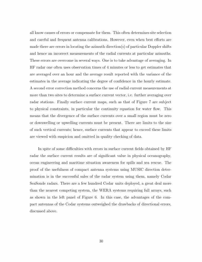
all know causes of errors or compensate for them. This often determines site selection
and careful and frequent antenna calibrations. However, even when best efforts are
made there are errors in locating the azimuth direction(s) of particular Doppler shifts
and hence an incorrect measurements of the radial currents at particular azimuths.
These errors are overcome in several ways. One is to take advantage of averaging. In
HF radar one often uses observation times of 4 minutes or less to get estimates that
are averaged over an hour and the average result reported with the variance of the
estimates in the average indicating the degree of confidence in the hourly estimate.
A second error correction method concerns the use of radial current measurements at
more than two sites to determine a surface current vector, i.e. further averaging over
radar stations. Finally surface current maps, such as that of Figure 7 are subject
to physical constraints, in particular the continuity equation for water flow. This
means that the divergence of the surface currents over a small region must be zero
or downwelling or upwelling currents must be present. There are limits to the size
of such vertical currents; hence, surface currents that appear to exceed these limits
are viewed with suspicion and omitted in quality checking of data.
In spite of some difficulties with errors in surface current fields obtained by HF
radar the surface current results are of significant value in physical oceanography,
ocean engineering and maritime situation awareness for spills and sea rescue. The
proof of the usefulness of compact antenna systems using MUSIC direction deter-
mination is in the successful sales of the radar system using them, namely Codar
SeaSonde radars. There are a few hundred Codar units deployed, a great deal more
than the nearest competing system, the WERA systems requiring full arrays, such
as shown in the left panel of Figure 6. In this case, the advantages of the com-
pact antennas of the Codar systems outweighed the drawbacks of directional errors,
discussed above.
30

2.4 Summary
2.4.1 Findings
1. Many elements of compressed sending have been used for decades, and benefits
of using a CS approach in several application areas is clear. In some cases,
e.g., JPEG photographic compression, elementary sparse reconstruction was
used with simple algorithms, but other fields, such as radio astronomy and
coastal radar, also applied sparse sampling and complex algorithms to overcome
hardware limitations.
2. Compressed sensing always involves tradeoffs, most often accepting decreased
SNR in exchange for maintaining resolution requirements despite limitations
on measurement resources, or in exchange for a reduction in data volume.
2.4.2 Recommendations
1. Evaluation of CS algorithms proposed for radar should consider some or all
of the following assessment methods suggested by the MUSIC case discussed
here:
(a) A candidate CS algorithm application must be shown to fulfill the basic
requirements, such as illustrated above for MUSIC, for a sufficiently large
portion of the operation time.
(b) The CS algorithm must be needed for superior performance (e.g. proba-
bility of detection and false alarm rate) or by allowing superior implemen-
tation of a sensor concept, such as the MUSIC applications allows the use
of compact radar sites.
(c) The CS application algorithm must be compared comprehensively with
alternative techniques, as shown in Figure 9.
31

(d) A candidate CS algorithm application must demonstrate the ability to
cope with difficult and anomalous situations when requirements may not
be strictly met.
32

3 COMPRESSED SENSING TUTORIAL
3.1 Sparse Images.
Various sources of compressibility appear in the literature. Most commonly, and
most relevantly for us, an image is compressible because it is nearly sparse. We
usually model an N -pixel image as a (column) vector in RN , with one coordinate
per pixel.1 Such a vector is said to be “sparse” relative to the natural basis of unit
vectors ei of RN if most of its coordinates are zero. Formally, we define the sparsity
‖x‖0 of a vector
x = (x1, x2, . . . , xN)T = x1e1 + x2e2 + · · · + xNeN (3-9)
to be the number of non-zero coordinates of x:
‖x‖0 = #i : 1 ≤ i ≤ N, xi 6= 0. (3-10)
[See below for the significance of the notation ‖·‖0 and the properties of this function.]
We say x is K-sparse if ‖x‖0 ≤ K. A typical example is a night sky with few bright
spots against an entirely dark background. If we regard RN geometrically as an
N -dimensional space then the K-sparse vectors constitute the union of the
(
N
K
)
=N !
K!(N −K)!=
N
K
N − 1
K − 1
N − 2
K − 2· · · N − K + 1
1(3-11)
coordinate subspaces of dimension K.
To specify a K-sparse image of length N , we must choose one of these subspaces
and then a vector in one of them.2 Given the subspace and β bits per word, it takes
1For color images each pixel may naturally correspond to more than one coordinate; for example,a 24-bit color pixel consists of three 8-bit picture elements, one for each primary color.
2This slightly overcounts the total of K-sparse images because an image of sparsity strictly lessthan K is counted multiple times. But this has a negligible effect on the final result, as can be seenby using the same technique to count for each k ≤ K the images of sparsity exactly k, and thensumming over k.
33

βK bits to specify its K pixels. The choice of subspace requires log2
(
NK
)
bits. Each
of the K factors in the formula (3-11) for(
NK
)
is between N/K and N ; hence
K log2
N
K≤ log2
(
N
K
)
≤ K log2 N. (3-12)
We deduce that it takes at least
(
β + log2
N
K
)
K (3-13)
bits to represent a K-sparse image. We must therefore acquire at least this many
bits of information about the image to reconstruct it. CS will let us come within a
small factor of this lower bound.
To be sure, very few images of interest are exactly K-sparse with K small
enough for CS to exploit. But the linear-algebra framework of CS accommodates
generalizations in two directions that together recover the most common and widely
studied class of compressible images.
One necessary generalization is from exactly K-sparse to approximately K-sparse
images, that is, images of the form x = x + n where x is K-sparse and n is a small
“noise” vector. Noise is inescapable in any actual application, not just in the mea-
surement but also in the image itself (even the night-sky background is not perfectly
dark). In some applications the noise is modeled as coming from a Gaussian distri-
bution, with small Euclidean (a.k.a. `2) norm
‖n‖2 =√
n21 + · · · + n2
N . (3-14)
Another common model is a power law, where there are many point sources but
their magnitude decays rapidly enough that the m-th largest coordinate is bounded
by some multiple of m−1/r (with constant r > 0); then for each ε > 0 there are only
O(ε−r) coordinates satisfying |xi| > ε. If r is small enough, then the K-sparse vector
that retains only the top K coordinates of x approximates x to within O(K−θ) for
34

some θ > 0. For example, if we use the Euclidean norm, and r < 2, then the noise
magnitude is bounded by a multiple of the convergent sum
√
∑
m>K
(m−1/r)2 ∼(
∫
∞
m=K
m−2/r dm
)1/2
= O(K1
2−
1
r ), (3-15)
so θ = (1/r) − (1/2). Whatever the nature of the noise n, we are usually satisfied
with recovering a sparse vector x to within an error comparable with the size of n,
and still regard x as compressible (this time with lossy compression).
The second generalization lets us replace the basis vectors e1, e2, . . . , eN by an
arbitrary set of N ′ typical image elements v1, v2, . . . , vN ′, of which the image x is a
K-sparse linear combination:
x = c1v1 + c2v2 + · · · + cN ′vN ′ with ‖c‖0 ≤ K. (3-16)
For example, vi might be a wavelet basis for RN , such as the one used for JPEG-
2000. We write the expansion (3-16) in matrix form as
x = Ψc, (3-17)
where Ψ is the matrix formed from the N ′ columns vi, and c = (c1, c2, . . . , cN ′)T is the
coefficient vector. The CS framework does not require that the vi be orthogonal, or
even independent: any finite collection (“dictionary”) of N ′ vectors will do. Usually
these vectors linearly span RN , so that N ′ ≥ N , but still N ′ will not exceed N by
more than a small factor. For example, the dictionary might consist of both the unit
vectors and a wavelet basis, in which case N ′ = 2N and Ψ is the concatenation of
the N × N identity matrix and the N × N orthogonal matrix corresponding to the
wavelets.
Combining these two generalizations yields x = Ψc + n, where c is sparse, and
n is a noise vector as above, possibly modeled by a Gaussian or the tail of a power
law, or some combination of the two.
35

3.2 Linear Measurements
A camera measures each of the N coordinates (or pixels) xi of an image x separately.
CS replaces these N measurements with measurements of M linear combinations
yj =∑N
i=1 ai,jxi (1 ≤ j ≤ M); in matrix form,
y = (y1, . . . , yM)T = Ax (3-18)
where A is the matrix with M rows of length N , the j-th row consisting of the
coefficients ai,j of the j-th measurement. If M < N then we cannot solve the linear
system (3-18) for x by inverting A, but this system might still determine x uniquely
under the additional condition that x is K-sparse. Indeed this is the case for all
K-sparse x precisely when the “spark” of A exceeds 2K, that is, when any 2K
columns of A are linearly dependent (Donoho, 2006b; Cande et al., 2006) [20, 15];
equivalently when the kernel (column nullspace) of A contains no 2K-sparse vectors
other than 0.3 If x is K-sparse with respect to the N ′ columns of some matrix Ψ,
then our equation becomes
y = (y1, . . . , yM)T = AΨc, (3-19)
to be solved for a K-sparse vector c of length N ′; but this is a problem of the same
form as (3-18) with (A, x) replaced by (AΨ, c), so the same analysis applies: the
solution, if it exists, is always unique if and only if AΨ has spark > 2K.
3The reader familiarwith the theory of error-correcting codes will recognize this “spark” criterionas the condition that kerA be a linear code of minimal distance > 2K, that is, a K-error-correctinglinear code over R. In this context ‖x‖0 is the Hamming weight of x. As in the coding-theorysetting, the proof uses the fact that the Hamming weight, though not a vector-space norm (because‖cx‖0 = ‖x‖0, for c 6= 0, not |c| · ‖x‖0), does satisfy the triangle inequality ‖x+x′‖0 ≤ ‖x‖0 +‖x′‖0,together with the property that every vector of weight ≤ 2K can be written as the sum of twovectors of weight at most K. (This connection appears in Ackaya and Tarokh (2007) [4]).
36

3.3 Limitations of the Exact y = Ax Mmodel
As it stands this y = Ax model is not satisfactory for practical use, for several
reasons:4
i) there is no efficient algorithm known for testing whether the spark of a given matrix
(here A or AΨ) exceeds 2K;
ii) even if a sparse solution of y = Ax is known to exist, there is no efficient algorithm
known to find it (for example, it is wildly impractical to try all(
NK
)
or(
N ′
K
)
possible
coordinate subspaces);
iii) Even if a solution exists it might not be numerically stable: a small change in y
might move x to an entirely different subspace.5 For that matter, the spark condition
is itself not numerically stable, because the spark of a matrix A can drop drastically
if A is perturbed.
This last difficulty is related with our earlier observation that real images and
real-valued measurements are inevitably beset by noise: not only does x differ from
a sparse vector x by some noise vector n, but even our observation A(x + n) is not
exact, so we observe only a vector
y = A(x + n) + ∆y = Ax + A · n + ∆y, (3-20)
degraded by some further noise ∆y (which may have various possible sources, ranging
from thermal noise to inexact calibration to roundoff errors in digitization). Our task,
then, is to approximately recover a K-sparse vector x given that (3-20) holds for some
4When N ′ = N , the first two difficulties can be overcome by choosing A of a special form. Forexample, for M > 2K one can use a Vandermonde matrix, with ai,j = αj−1
i for some distinctα1, . . . , αN ; then yj is the T j−1 coefficient of the power series of a rational function
∑
i xi/(1−αiT )of degree at most K, which can be recovered in time polynomial in K, as by the Berlekamp-Masseyalgorithm. (Again this corresponds to a classical construction in coding theory, here the Reed-Solomon codes.) But this approach is not available when N ′ > N because each row of A must bein the row span of a given matrix Ψ).
5Indeed a generic matrix A satisfies the spark condition provided M ≥ 2K, but this wouldcontradict our lower bound (3-13) on the number of bits needed to encode a K-sparse vector unlessβ is large enough to absorb the log(N/K) penalty; this already suggests that the spark conditionis not sufficient to achieve real-world CS.
37

known A and y (with y of length M N) and some upper bounds on the size of
the error vectors n and ∆y.
In the CS literature, this task is typically performed as follows:
• The spark condition on A is replaced by a stronger condition, called the
“restricted isometry property” (RIP), that is numerically stable and gives acceptable
bounds on how far any solution of (3-20) can be from the desired x when ‖x‖0 ≤ K.
• An even stronger condition on A (nearly orthogonal columns) is shown to im-
ply RIP, and to hold for randomly chosen A provided that M exceeds a sufficiently
large multiple of K(1 + log2(N/K)); moreover this condition can be tested in poly-
nomial time (MN2 multiplies, fewer if ATA is computed using techniques for matrix
multiplication).
• The solution of (3-20) is reduced, to within acceptable error, to optimization
problems for which practical algorithms are known.
The vagueness of the phrasings “numerically stable”, “acceptable”, and “suf-
ficiently large” is intentional. In each case there are proofs of inequalities with
constants that at least in principle can be made explicit. Actual implementation and
evaluation of CS often requires more precision in these constants than the literature
provides. There are various sources for this imprecision: theoretical guarantees are
by definition worst-case estimates that often understate practical performance; pub-
lished results may be stated for a wide class of problems, making them weaker than
necessary for a given case of interest; and finding the correct worst-case constant
may be a difficult mathematical problem that is not yet fully understood. Still, in
some cases it can be shown that the known estimates are not too far from the truth;
for instance, the guaranteed M might exceed K + β−1 log2(N/K) by a larger factor
than necessary, but it can never fall below K + β−1 log2(N/K).
38

Likewise “practical algorithms” means algorithms that are not much worse than
the algorithms used for traditional signal processing, but again “not much worse”
is a vague phrase that leaves open the question of just how much more effort CS
processing requires. This is still the topic of ongoing research, and may involve
tradeoffs against the choice of approximation to the true x.
3.4 The Restricted Isometry Property
Recall that a linear map A : RN→RN is an “isometry” if it preserves Euclidean
distances; equivalently, if ‖Ax‖2 = ‖x‖2 for every x in RN . In particular, such a
map has zero kernel (that is, Ax 6= 0 unless x = 0), and Ax cannot be close to Ax′
unless x is close to x′. For these properties, it would be enough for A to satisfy
(1 − δ)‖x‖2 ≤ ‖Ax‖2 ≤ (1 + δ)‖x‖2 (3-21)
for some positive δ < 1, as happens for instance when A is a diagonal matrix each
of whose diagonal entries is in the interval [1 − δ, 1 + δ]. We might call such A
an “approximate isometry” with parameter δ. If M < N then even approximate
isometries from RN to RM cannot exist, because every linear map RN→RM has
nonzero kernel. However, there are linear maps A : RN→RM that satisfy (3-21) for
all sparse vectors x.
More precisely, we say A satisfies the restricted isometry property (abbreviated
RIP) of order k if there exists some δk < 1 such that
(1 − δk)‖x‖22 ≤ ‖Ax‖2
2 ≤ (1 + δk)‖x‖22 (3-22)
holds for all k-sparse vectors x. In particular, if x 6= 0 then Ax 6= 0, so this property
implies that the spark of A exceeds k. In our setting we take k = 2K and deduce
that if A satisfies the RIP of order 2K then y = Ax has at most one K-sparse
39

solution x.6 Moreover, unlike the “spark” approach, the RIP criterion is numerically
stable: even if Ax′ does not exactly equal Ax we still have
‖x − x′‖22 ≤
1
1 − δ2K‖Ax− Ax′‖2
2. (3-23)
Thus, if we observe y = Ax + ∆y with ‖∆y‖2 < ν, and find some K-sparse x with
‖y −Ax‖2 < ν, then ‖A(x− x)‖2 is
‖Ax− Ax‖2 = ‖(y − Ax) − (y − Ax)‖2 ≤ ‖y − Ax‖2 + ‖y − Ax‖2 < 2ν
(using the triangle inequality in the penultimate step), so from (3-23) we deduce —
provided x is also K-sparse as expected — that
‖x− x‖ <2
(1 − δ2K)1/2ν. (3-24)
The other side of the inequality in the RIP definition (3-22) then yields
‖x− x‖2
‖x‖2<
2
(1 − δ2K)1/2
ν
‖x‖2≤ 2
√
1 + δ2K
1 − δ2K
ν
‖Ax‖2, (3-25)
which bounds the SNR (signal-to-noise ratio) in the recovered x in terms of the
bound ν/‖Ax‖2 on the SNR of the observation.
This leads us to ask:
1. Given N , k, and δk, how small can M be for a matrix A that satisfies the RIP
of order k?
2. How to construct such A?
3. Given A, how to find a sparse approximate solution of Ax = y?
4. How is the accuracy affected by noise in the image, rather than the observation
(n rather than ∆y in (3-20))?
6Proof: if x and x′ are K-sparse vectors with Ax = Ax′ then A(x−x′) = 0 with ‖x−x′‖0 ≤ 2K,so x − x′ = 0 and x = x′ as claimed.
40

The answers are known to within constant factors:
1) Provided k ≤ N/2, the minimal M is between ck log2(N/k) and Ck log2(N/k),
for some positive constants c, C depending only on δk. The expression k log2(N/k)
arises, as in (3-13), from the number of hyperplanes that must be distinguished. The
best values of c, C are not yet known in most cases.
2,3) Explicit constructions are hard but not necessary: provided C is large
enough, a random matrix will almost certainly satisfy the desired RIP.7 Assuming
this RIP, several practical approximation algorithms are known. Improvements are
again a topic of ongoing research. We give further details below.
4) CS is much more sensitive to random (as opposed to sparse) noise in x than
in Ax: the RIP bound (3-22) controls the size of ‖Ax‖2/‖x‖2 only for sparse x; if
x is allowed to vary randomly over RN , the ratio is typically of order√
N/M , so
CS incurs a degradation of N/M in the SNR ratio of the image (Arias-Castro and
Eldar, 2011) [6].
3.5 Finding RIP Matrices with Small M
Recall that if A satisfies the RIP of order k then M > ck log(N/k), and we want
such matrices with M < Ck log(N/k). The problem of explicitly constructing such
matrices remains unsolved. Fortunately it is not necessary to give a formula for A:
we can choose its entries randomly; and indeed this approach is the only known way
to attain M as small as some multiple of log(N/K). The CS literature contains
various results along these lines, depending on what probability distribution is used.
7This is again reminiscent of the theory of error-correcting codes: for some parameter ranges,the best existence result known is the Gilbert-Varshamov (GV) bound, obtained by analyzing thebehavior of random codes.
41

Most easily, each entry can be +1/√
M or −1/√
M with equal probability. More
generally, the columns can be independently chosen from the uniform distribution
on the unit sphere;8 or the rows can be chosen from the uniform distribution on the
sphere of radius√
N/M . More generally yet, the rows or columns can be chosen
from any “subgaussian isotropic distribution”: a probability distribution on RM or
RN whose coordinates have zero pairwise correlations and for which the probability
of a vector of norm > T is smaller than 12e−BT 2
for some B > 0 (that is, with tails
bounded by some Gaussian distribution). In each case the resulting matrix is known
to satisfy the RIP of order k and parameter δ with probability at least
1 − 2 exp(−cδ2M) (3-26)
provided that
M ≥ Cδ−2k(1 + log(N/k)). (3-27)
Here c, C are positive constants depending only on B. Thus, once these constants are
known it is enough to make M a large enough multiple of K log(N/K) for the random
matrix A to almost certainly satisfy the needed RIP. Again the known proofs provide
explicit constants c, C in (3-26,3-27), but the best constants are not known, and might
depend on how much is known or assumed about the probability distributions used
to generate A.
3.6 Sparse Recovery (SR)
When A satisfies the RIP of order 2K with a small enough δ (for example δ = 0.3),
it is feasible to recover a K-sparse vector x exactly from an exact measurement Ax,
and approximately from an approximate measurement Ax + ∆y. This is done by
finding, in the set B of all x consistent with the measurement, the one that minimizes
8A standard trick for doing that is to first choose each of M real numbers a1, . . . , aM from thesame Gaussian distribution centered at 0, and then divide the resulting vector (a1, . . . , aM) by its`2 norm.
42
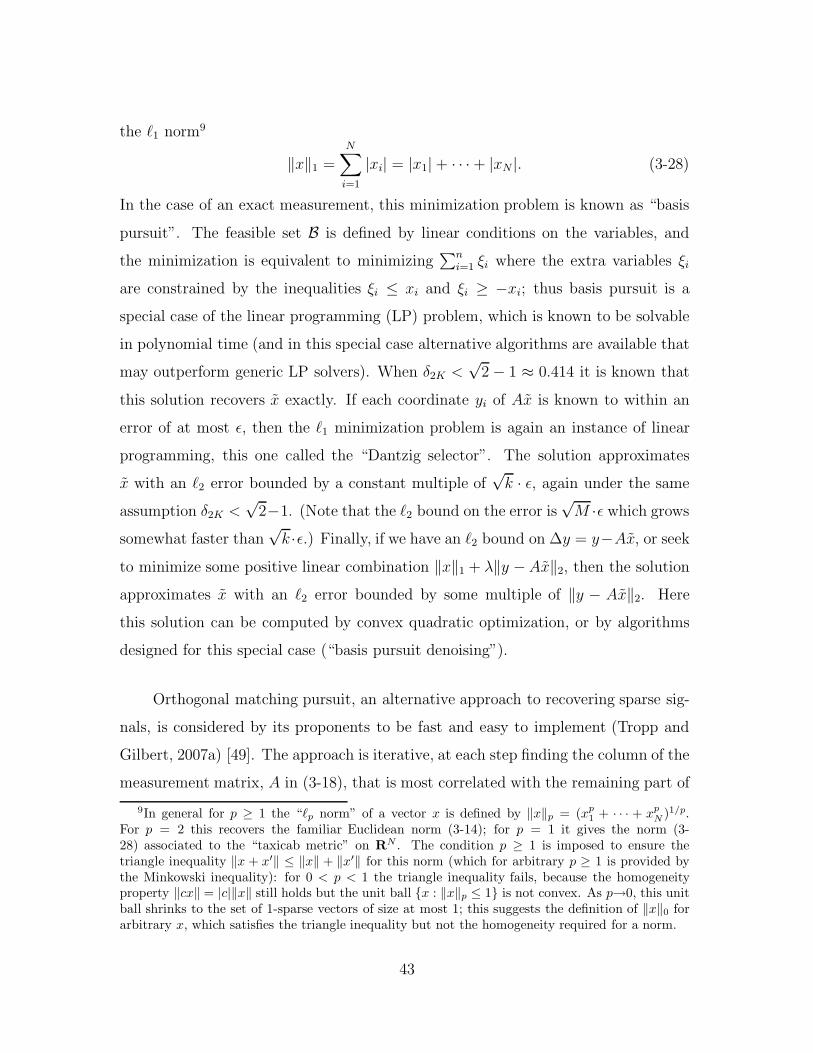
the `1 norm9
‖x‖1 =N
∑
i=1
|xi| = |x1| + · · · + |xN |. (3-28)
In the case of an exact measurement, this minimization problem is known as “basis
pursuit”. The feasible set B is defined by linear conditions on the variables, and
the minimization is equivalent to minimizing∑n
i=1 ξi where the extra variables ξi
are constrained by the inequalities ξi ≤ xi and ξi ≥ −xi; thus basis pursuit is a
special case of the linear programming (LP) problem, which is known to be solvable
in polynomial time (and in this special case alternative algorithms are available that
may outperform generic LP solvers). When δ2K <√
2 − 1 ≈ 0.414 it is known that
this solution recovers x exactly. If each coordinate yi of Ax is known to within an
error of at most ε, then the `1 minimization problem is again an instance of linear
programming, this one called the “Dantzig selector”. The solution approximates
x with an `2 error bounded by a constant multiple of√
k · ε, again under the same
assumption δ2K <√
2−1. (Note that the `2 bound on the error is√
M ·ε which grows
somewhat faster than√
k ·ε.) Finally, if we have an `2 bound on ∆y = y−Ax, or seek
to minimize some positive linear combination ‖x‖1 + λ‖y −Ax‖2, then the solution
approximates x with an `2 error bounded by some multiple of ‖y − Ax‖2. Here
this solution can be computed by convex quadratic optimization, or by algorithms
designed for this special case (“basis pursuit denoising”).
Orthogonal matching pursuit, an alternative approach to recovering sparse sig-
nals, is considered by its proponents to be fast and easy to implement (Tropp and
Gilbert, 2007a) [49]. The approach is iterative, at each step finding the column of the
measurement matrix, A in (3-18), that is most correlated with the remaining part of
9In general for p ≥ 1 the “`p norm” of a vector x is defined by ‖x‖p = (xp1
+ · · · + xpN )1/p.
For p = 2 this recovers the familiar Euclidean norm (3-14); for p = 1 it gives the norm (3-28) associated to the “taxicab metric” on RN . The condition p ≥ 1 is imposed to ensure thetriangle inequality ‖x + x′‖ ≤ ‖x‖ + ‖x′‖ for this norm (which for arbitrary p ≥ 1 is provided bythe Minkowski inequality): for 0 < p < 1 the triangle inequality fails, because the homogeneityproperty ‖cx‖ = |c|‖x‖ still holds but the unit ball x : ‖x‖p ≤ 1 is not convex. As p→0, this unitball shrinks to the set of 1-sparse vectors of size at most 1; this suggests the definition of ‖x‖0 forarbitrary x, which satisfies the triangle inequality but not the homogeneity required for a norm.
43

Figure 10: Percent of signals with sparsity K recovered) versus the number of mea-surements, M, recovered orthogonal matching pursuit (Adapted from Tropp andGilbert (2007a) [49]). The dimension of the signal space was N = 1024. Empiricalrecoveries are much more efficient than the theoretical guarantee (Tropp and Gilber,2007b) [50].
the signal, x. The contribution of that column to x is subtracted before proceeding
to the next iteration. Numerical simulations to test the recovery guarantee in Tropp
and Gilbert (2007b) [50] used normalized, independent Gaussians for columns of A
and determined how many measurements, M , were in fact needed to recover arbi-
trary random signals x of dimension N and sparsity K. As in other sparse recovery
cases, many fewer measurements are needed than the worst case guarantee (Fig. 10).
For instance, with K = 5 about 130 measurements are needed to recover the first
signal element and ≈ 280 are needed to get them all, according to the guarantee.
In practice, these numbers decrease to M ≈ 10 and M ≈ 70. That is, even for this
algorithm, full recovery required 15 times more measurements than the sparsity.
44

3.7 Noisy Images
CS is more sensitive to random noise in the image x than in the measurements that
constitute Ax. The phrase “random noise” is intended to exclude the case that x is
not sparse but its nonzero coordinates are distributed according to a power law. In
the power-law case, x is not K-sparse but is increasingly close to K ′-sparse vectors
as K ′ increases. In this case A likely still has RIP of order 2K ′ for K ′ somewhat
greater than K, albeit with worse (i.e. larger) parameters δ2K′; so the SR algorithms
can still approximate the K ′-sparse approximations to x, and thus come reasonably
close to x itself.
But when the noise n is not concentrated in K ′ coordinates but spread evenly
throughout the image, the SR techniques cannot adapt as well. Indeed, an RIP
matrix A typically takes n to a vector whose `2 norm ‖A · n‖2 exceeds ‖n‖2 by a
factor of about√
N/M .10 If we can tolerate the resulting degradation of the signal-
to-noise ratio by a factor of N/M , then we can simply include this A · n term in
∆y and recover an approximate x as before. But if the SNR of the image is already
too small, then we must scale back the compression ratio of N/M , and with it our
ambitions for using CS to reduce the costs of acquiring an N -pixel image.
After noting that most CS literature does not consider noise and those that
do assume only measurements noise, Arias-Castro and Eldar (2011) [6] analyze the
most realistic situation, sensor, ns, and measurement, nm, noise,
y = A(x + ns) + nm . (3-29)
If A is an M × N matrix, they show that an equivalent statement is
y = Bx + n1 (3-30)
10A typical entry of A ·n has contributions of size about M−1/2‖n‖2 from all N coordinates, notjust K of them. Since the RIP guarantees that ‖Ax‖2 is comparable with ‖x‖2 for K-sparse x, thissuggests a ratio ‖A · n‖2/‖n‖2 of about N/K, which is roughly consistent with the actual
√
N/Mestimate because M is within logarithmic factors of K.
45

where the noise variance of n1 is σ21 = (σ2
m+(N/M)σ2s , where σ2
m is the measurement
noise variance and σ2s is the sensor noise variance. If σs is comparable to σm, sensor
noise will degrade the signal-to-noise ratio (SNR), severely so, when M N . This
result illustrates the fundamental tradeoff between measurement effort and SNR
inherent in most applications of CS.
3.8 Two Examples of Compressed Sensing
The first example applies CS techniques to identify rare alleles efficiently, and the sec-
ond uses sparse reconstruction to estimate the cosmic microwave background where
it is obscured by our galaxy. The first appears to be on a useful path. Though the
second is questionable, the underlying approach should be kept in mind for possible
DoD applications.
3.8.1 Identification of rare alleles
Here we outline a simple example of compressed sensing, inspired by the paper
”Identification of rare alleles and their carriers using compressed sensing” (Shental
et al., 2010) [47]. The authors consider the problem of identifying members of a
population who have a rare genetic variant. One method for finding these individuals
is to sequence the entire population, and then by brute force identify those with the
rare alleles. But this is expensive. It has long been known that if you are instead
interested in simply analyzing the frequency of occurrence of the rare allele, this can
be done by pooling all of the DNA from the population, and measuring the frequency
of the rare allele (See Norton et al. (2002) [35]). But with such a measurement, one
has no way of figuring out precisely which individuals possess the rare alleles.
To do this, Shental et al. (2010) [47] argue that we should proceed as follows.
Let us denote the genotypes of the population by x, which is a vector of length N ,
46

where the ith component, xi, gives the genotype of the population, and N is the size
of the population. Denote the common allele by A and the rare allele by B. Each
person has either 0, 1 or 2 copies of the rare allele. Since the allele in question is
rare, by construction the vector x is sparse–only a small fraction of its entries are
nonzero. In fact, the more rare the allele, the more sparse the entries will be.
Now, we would like to determine which members of the population have the
rare allele; we will do this by breaking the population into pools, and measuring the
frequency of the rare allele in each pool. To represent this in mathematical form we
construct the sensing matrix M : each entry mij is equal to one if the jth individual
is in the ith pool, and it is zero otherwise. For each pool, we measure the frequency
fi of the rare allele. Thus, we have arrived at the mathematical problem
f = Mx
where f is the vector of frequencies that are measured in the different pools.
The theory of compressed sensing requires that for the solution x to be unique,
the matrix M must be sufficiently sparse and obey the restricted isometry property
(RIP). To require this, we demand that M be a Bernoulli matrix, whose entries are
either 0, 1 with probability 0.5. Such a matrix obeys the RIP (Donoho, 2006b) [20].
Other designs of the sensing matrix are possible, which might be more economical11,
but this example demonstrates that the pooling idea is theoretically possible.
The idea of using compressed sensing to find the individuals with rare alleles is
a beautiful one, but as always the devil is in the details. To understand whether it
can actually work it is necessary to consider the noise in the measurements. There
are several different sources of noise that are discussed in the Shental paper that
could be significant:
11For example the Shental paper discusses a matrix with only O(√
N) nonzero entries per rowand argues that this also works.
47

1. First, when pooling the DNA, it is assumed that an equal amount of DNA
is taken from each person. If there were variability in this amount it would
significantly contaminate the measurements.
2. Sequencing requires PCR amplification of the different individuals, and it is
assumed that PCR affects every individual in the same way. If not, the am-
plified pools will contain different amounts of the allele in accordance with an
individual’s amplification propensity, which will contaminate the formalism. It
has been previously shown that the number of reads of a given genetic region
can depend on factors like the GC content of that region, and can depend on
experimental conditions. The distribution of read length has been previously
modeled as a Gamma distribution (rightly or wrongly!) (Prabhu and Pe’er,
2009) [40].
3. The frequency of each pool is obtained by computing the ratio of the number of
reads of the are allele to the total number of reads in that pool. In reality, if a
specific locus contains a small enough number of reads the frequency will itself
have an uncertainty associated with it due to sampling noise. Additionally, the
sequencer will itself introduce sequencing errors.
The authors deal with these uncertainties by formulating a compressed sensing
problem with noise–instead of demanding an exact solution to f = Mx, they require
an approximate one where the error is suitably bounded according to the noise levels
in question. Under suitable conditions for the size of the different noise factors,
they show through simulations that the compressed sensing framework does allow
determination of the rare allele individuals. Of course whether or not this works
in practice depends on the actual sources of noise in an actual experiment, both
the read errors in the sequencer, as well as the sampling errors in extracting DNA
from each individual. Additionally, the method using the Bernoulli matrix as the
sensing matrix requires that each pool contains of order 1/2 the people in the entire
48

population. This might be difficult to carry out in practice.
3.8.2 Inpainting the cosmic microwave background
We survey an application of CS/SR-inspired ideas to the Cosmic Microwave Back-
ground (CMB) measurement problem which in turn led to yet another series of
mathematical results. The application is from Abrial et al.(2008) [3] and concerns
the Wilkinson Microwave Anisotropy Probe (WMAP) data.
The CMB inpainting problem is to render an accurate full-sky temperature
anisotropy map, ∆T (φ, θ), of the universe as observed from Earth in all directions
where
T (φ, θ) = T0 + ∆T (φ, θ).
The difficulty is that the measured data incorporates “voids” arising from the in-
terference from “nearby” sources as well as from our own galaxy which effectively
prevent direct measurements in a substantial “equatorial” region (Fig. 11). With
the new data sets coming in from the Planck Mission, solving the inpainting prob-
lem is seen as an important step in determining fundamental constants from the
experimental data.
Under the assumption that ∆T = ∆T (φ, θ) is well approximated by a sparse
function when expanded relative to the basis of spherical harmonics, CS/SR inspired
ideas have been used to fill in the voids. The approach is to view the inpainting
problem as an instance of the following abstract problem.
Suppose that L2(ν) is the Hilbert space of square-integrable functions (real or
complex valued) over a probability measure space (M, ν). Suppose 〈φi : i ∈ N〉 is an
orthonormal basis, N ∈ N and
f : M → C
49
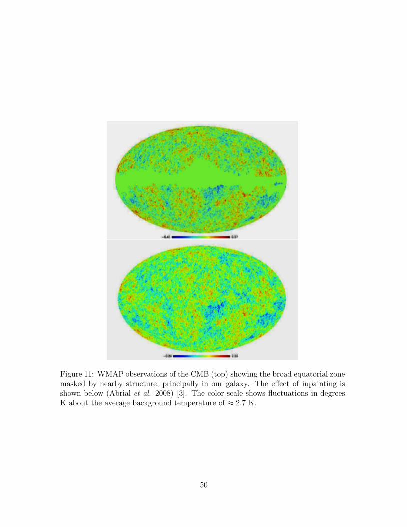
Figure 11: WMAP observations of the CMB (top) showing the broad equatorial zonemasked by nearby structure, principally in our galaxy. The effect of inpainting isshown below (Abrial et al. 2008) [3]. The color scale shows fluctuations in degreesK about the average background temperature of ≈ 2.7 K.
50

is function in L2(ν). For a given s < N , f is s-sparse and N band-limited relative
to the given basis if
f = ΣNk=1ciφi
and the set of ci such that ci 6= 0 has size at most s. The problem is to recover f by
sampling f at points chosen at random. If B bounds the values |φi(x)| for all x ∈ M
and i ≤ N (these are the L∞-norm bounds), then choosing m points at random
where
m ≥ s · B2 · log4 N
makes recovery provably possible with high probability. The connection with the
conventional CS/SR schemes is that the m×N matrix (φj(xi)), given by evaluating
the j-th basis element at the i-th point, is proved with high probability to have the
required instance of the Restricted Isometry Property (RIP), [R]. The remarkable
fact is that as a consequence of the RIP property, f , is the only s-sparse solution to
the under-determined linear system:
A · ~X = ~y
where A is the m×N -matrix (φj(xi)) and ~y = (f(xi)); moreover it is the unique vector
of minimum l1-norm among all possible solutions (sparse or not) to this equation
(Candes et al., 2006) [15]. Thus, the recovery of f is a linear programming problem
which can be efficiently solved.
More generally, if g is a function which is well-approximated by an s-sparse,
N band-limited, function f , then the same methodology works to recover a good
approximation to g.
One can also use a weight, w(x) (with w(x) ≥ 0 and∫
w(x)dν = 1), provided
the induced measure preserves orthogonality of the basis functions. Then the original
bound B is replaced by
sup|φi(x)/[w(x)]1/2| : i ≤ N, x ∈ M.
51

In the CMB context, the space of functions is L2(S2) of functions defined on the
unit sphere in 3-dimensions with the uniform measure, and the basis is that given by
the (normalized) spherical harmonic functions, Y ml where m and l are integers with
l ≥ 1 and |m| ≤ l. Thus
∆T (φ, θ) = Σ∞
l=0Σlm=−l al,mY m
l (φ, θ)
The function ∆T has an associated power spectrum
S∆T (l) = Σlm=−l|al,m|2
which is important in evaluating cosmological models and for determining key cos-
mological parameters.
Sparsity up to the m-degeneracy is independent of the choice of polar axis
(choice of “north”). Even assuming the predicted “approximate l-sparsity” is such
that the function ∆T is in theory well approximated by sparse functions relative
to any choice of the axis for θ, the requisite bound B is useless. However one can
replace the uniform measure by a weighted measure (preserving the orthogonality of
the basis functions).
In angular coordinates the uniform measure is (1/4π) sin θdθdφ, where θ, is the
polar angle. The uniform measure in the angular coordinates, (1/2π2)dθdφ, is still
an orthogonalization measure for the original basis, and, further, the (non-trivial)
estimate
(sin θ)1/2|Y ml (φ, θ)| ≤ l1/4
gives (by the methodology described above) a sampling requirement,
m ≥ sN1/4 log4 N ,
for exact recovery (with high probability) for an s-sparse function f (Rauhut and
Ward, 2011) [42].
52

By a fortunate coincidence randomly choosing points relative to this measure
concentrates points at the poles and away from the equator, matching the general
character of the data sets (so here one is specifying “north” so that the Milky Way
occupies the equatorial field of view).
In Burq et al.(2011) [13] a substantial additional improvement is obtained by
changing the weighted orthogonalization measure to [tan θ]1/3dθdφ and proving the
requisite bound which now converts to the sampling requirement of
m ≥ sN1/6 log4 N
for exact recovery (with high probability) for an s-sparse function f .
Choosing points with this measure concentrates points at the poles and the
equator , apparently not very useful for the inpainting problem. But, the rather
sophisticated techniques used to establish bounds yielding improvement, specifically
in proving the kinds of sufficient L∞-norm estimates as indicated above, generalize
to the much more abstract setting given by functions defined on surface of a convex
solid of revolution (Burq et al., 2011) [13].
But is this really an instance of CS/SR? If one looks at the actual numbers, the
pixel resolution of the WMAP data ranges from about .3 to .5 degrees depending
on the measured frequency. This gives a maximum pixel count of around 5 · 105.
Viewing the pixels as corresponding to the sampling points in the above schemes
then
5 · 105 ≥ s · N1/6 log4 N
using the most optimistic estimate from Burq et al. (2011) [13] and ignoring that
the corresponding sampling measure in this case concentrates the points at the poles
and equatorial region (the equatorial region is where the data are masked by noise).
The recovered multipole spectrum has nontrivial support uniformly in the interval
ranging from l = 100 to l = 1000 and so N ≥ 106 (and the CS/SR idealization would
53

require that N > m where m is the number of sampling points anyway). Thus
5 · 105 ≥ s · (106)1/6 log4(106) ≥ s · 15 · 105
which is impossible since s ≥ 1. Further, a sparsity of s ≤ 100 is completely in-
consistent with the recovered multipole spectrum even assuming the expansion in
spherical harmonics is such that only one basis basis function for each l-value is used
(so that sparsity in l corresponds to actual sparsity). Given the physical symmeties
of the problem there should be no preferred orientation and so the amplification of
the sparsity parameter given by the m-degeneracy very likely makes the situation
much worse.
In summary, the CS/SR idealization of the inpainting problem for the CMB
data from the WMAP mission seems very possibly to be so idealized as to be totally
irrelevant. This, however, does not mean that inpainting may not have use for some
DoD applications.
54

4 THE SINGLE-PIXEL CAMERA
One prominent application of CS is the single-pixel camera developed by Kelly and
Baraniuk of Rice University. Duarte et al. (2008) [21] describe the prototype, and a
startup company, InView, is marketing several versions of single-pixel infrared cam-
eras (http://www.
inviewcorp.com). To avoid using expensive focal plane arrays, each pixel of which
must detect infrared light, these devices use pseudo-random selections of micro mir-
rors to reflect light from an imaging system onto a single detector that is cheaper
and of higher performance than the focal plane arrays. Figure 12 shows the concept
schematically. InView is marketing their first models at prices 3 to 10 times less than
those of comparable ‘market leaders,’ which sell for $40,000 to $50,000. We also were
told that Lockheed Corp. is optimistic that it can develop an infrared camera that
will increase capability and decrease costs for DoD.
Duarte et al. (2008) [21] discuss theoretical tradeoffs, comparing the CS single-
pixel approach with a conventional multi-pixel array and a raster scan. Typically, a
CS image is formed by taking M =O(KP log2(N/K)) measurements, where K is the
image sparsity, and N M is the number of elements in the equivalent multi-pixel
array and raster scan. If 0 to D is the dynamic range of a pixel in a focal plane
array, Duarte et al. give ND/2 as the required dynamic range of the single-pixel
camera, assuming that the weakest signal occurs when only one of the N/2 mirrors
directed at the detector is illuminated and the strongest signal results from all N/2
mirrors being illuminated. For N = 1×10⁶ , or more, this is a very stiff requirement,
i.e. that the single detector have a dynamic range 5 × 10⁵ times that of a single
pixel in a mega-pixel focal plane array. On the other hand, if the light intensety is
relatively uniform across the image, they dynamic range required is around D√
N ,
or ∼ 103, higher than for the FPA. For a sample duration of T seconds, the mean
square counting error for the array is P/T , where P is the number of photons per
55

Figure 12: Schematic of single-pixel cameras developed by InView. The imagingsystem focuses on a digital micromirror device (DMD) consisting of a million micron-sized mirrors that are randomly selected so half reflect photons onto a single-elementinfrared detector, the output of which is sampled by an analog-to-digital (A/D)converter. Successive frames are formed different combinations of mirrors.
second on a pixel. This rises to NP/T for the raster scan and (3N−2)P/T for a basis
scan. For CS, Duarte et al. obtain 3C2NMP/T , where CN is the noise amplification
factor after reconstruction, implying that the CS measurement scheme would have
lower noise than the simple raster scale if M < N/3C2N .
Because these estimates are central to understanding the benefits and liabilities
of the single-pixel approach, below we present an alternate analysis that assumes the
scene of interest is relatively uniformly illuminated, as was also assumed by Duarte
et al. (2008) [21].
56

4.1 Focal-plane Array
Suppose the image consists of a set of N pixels with mean intensity (photons per
second) µi, where i = 1, ..., N indexes the pixels. Let yi represent the actual number
of photons collected by a pixel in a focal-plane over a measurement time T , and let
δyi = yi − 〈yi〉 represent the fluctuation of yi. This is a Poisson random variable
satisfying
〈yi〉 =⟨
δy2i
⟩
= µiT . (4-31)
Using δy and µ to denote the associated column vectors, we may write the covariance
matrix as
Cy =⟨
δy δyT⟩
= diag(µ)T . (4-32)
This equation expresses the fact that the photon counts are uncorrelated. We may
estimate the image in the obvious way,
µ =y
T(4-33)
and this estimator has a covariance
⟨
δµ δµT⟩
=1
Tdiag(µ) , (4-34)
indicating that our measurement uncertainty improves as the square-root of the
measurement time. This result agrees with Duarte et al., with the identification of
the quantity P = µ.
4.2 Raster Scan
Now suppose that a single detector is used to form an image by sequentially scanning
through the N pixels in raster fashion. The measurements yi obtained in this way
have mean and variance
〈yi〉 =⟨
δy2i
⟩
= µiT
N(4-35)
57

because the total measurement time T is subdivided into N measurement periods.
We now estimate the image using
µ =N
Ty (4-36)
and the estimated image has covariance
⟨
δµ δµT⟩
=N2
T 2
⟨
δy δyT⟩
=N
Tdiag(µ) , (4-37)
Thus, compared to the N -pixel focal plane array, the measurement sensitivity has
degraded by√
N . This is obvious, because we are collecting photons at an average
rate which is N times lower. This result also agrees with Duarte et al. (2008).
4.3 Basis Scan
In this case, the image is passed through a programmable mask (e.g., a DMD)
which may either pass or block the light for a particular pixel, before sending all
of the transmitted light to a single detector. A sequence of N masks is used to
allow image reconstruction without making any assumptions regarding sparsity. The
measurements are described by N independent Poisson random variables yi arranged
into a column vector y,
y =T
NΦµ + δy (4-38)
where the fluctuation vector δy = y − 〈y〉 has a covariance of
⟨
δy δyT⟩
=T
Ndiag(Φµ) . (4-39)
Here, the elements of the measurement matrix Φij = 0 or 1 represent the mask value
for pixel j during measurement i. Again, the N in the denominator arises from
subdividing the measurement time N ways. Duarte et al. take Φ to be
Φij =1
2(Wij + 1) (4-40)
58

or
Φ =1
2(W + O) (4-41)
where O is a matrix filled with ones and Wij = ±1 is the orthogonal Walsh or
Hadamard matrix, satisfying
W T W = NI (4-42)
where I is the identity matrix. For example, the Walsh matrix for N = 4 is
W = W T =
1 1 1 11 −1 1 −11 1 −1 −11 −1 −1 1
(4-43)
and the measurement matrix is
Φ = ΦT =
1 1 1 11 0 1 01 1 0 01 0 0 1
. (4-44)
Note that there is a small peculiarity in that pixel 1 is singled out for special treatment
in this scheme, since its light is always allowed to fall on the detector.
For this case of N measurements and N unknowns, the measurement equation
is invertible, so we estimate the image using the unbiased linear estimator
µ =N
TΦ−1y (4-45)
which has a covariance of
⟨
δµ δµT⟩
=N2
T 2Φ−1
⟨
δy δyT⟩
(Φ−1)T
=N
TΦ−1diag(Φµ)Φ−1. (4-46)
Note that if we set Φ = I , which is equivalent to a raster scan, we reproduce eqn. 4-37.
The inverse of the Walsh-derived measurement matrix may be shown to be
(Φ−1)ij =2
NWij − δi1δ1j . (4-47)
59

For a quick estimate of the covariance matrix, we assume the image is uniform enough
so that∑
j
Φijµj ≈N
2µ(1 + δi1) . (4-48)
This is exactly correct if the image is perfectly uniform, µi = µ for all i. However
our assumption is not particularly restrictive since each mask collects light from half
of the pixels, and the brightness variations across the image will tend to average out.
This gives
⟨
δµ δµT⟩
ij=
N
T
N∑
k=1
(
2
NWik − δi1δ1k
)
N
2µ(1 + δk1)
(
2
NWkj − δk1δ1j
)
=2N
Tµδij −
N
Tµδ1j +
2
Tµ − N
Tµδ1j
−N
Tµδi1 +
N2
2Tµδi1δ1j −
N
Tµδi1 +
N2
2Tµδi1δ1j
=2N
Tµ
[
δij +1
N− δi1 − δ1j +
N
2δi1δ1j
]
. (4-49)
Thus, apart from the expected peculiar behavior of pixel 1 (it is never turned off in
this measurement scheme, which makes it more difficult to determine its intensity),
we see that the sensitivity relative to a focal plane array has been degraded by the
factor√
2N + 2, or approximately√
2N for large N . Note that this result is also
worse than that for a raster scan with a single pixel, by the factor of√
2. This loss
presumably results from the DMD throwing half the photons away. Note also that in
the case of the raster scan, the noise of pixel i depends on the intensity of only that
pixel, rather than the average intensity in the image. In other words, the variance
for the raster scan is Nµi/T , rather than 2Nµ/T for the basis scan. This detail is
significant in the case that the image has a large contrast: the noise of the raster-scan
image will be lower in the dark regions, exactly where you would like to have lower
noise.
This result of 2Nµ/T disagrees with that stated by Duarte et al., who give a
variance of (3N − 2)µ/T .
60

4.4 Compressive Sampling
We now examine the case in which we pick M << N rows of the Walsh-Hadamard
measurement matrix Φ at random, and spend an equal time T/M performing mea-
surements for each of these rows. Thus we have
y =T
MΦµ + δy (4-50)
except that Φ is now an M×N matrix and y is the measurement vector of length M .
We make the assumption that the signal is K-sparse in the pixel basis, although any
other basis that is also incoherent with respect to the measurement basis could be
used equally well. To be more precise, we assume that the image is perfectly uniform
with the exception of K pixels, whose intensities are only slightly different than the
rest. If the k-th such pixel, located at position p(k), has an intensity of xk, we may
write
µi = µ
[
1 −K
∑
k=1
δi,p(k)
]
+
K∑
k=1
xkδi,p(k). (4-51)
In this form, the signal vector µ is the sum of a set of K +1 orthogonal basis vectors
which are incoherent with respect to the measurement basis; this is the standard
setup for CS. For simplicity, we will assume that xk − µ is small. This is essentially
the case analyzed by Duarte et al. (2008).
4.4.1 Cramer-Rao bound
The average photon count for each measurement is given by
λm ≡ 〈ym〉 =T
M
N∑
i=1
Φmiµi ≈T
M
N∑
i=1
Φmiµ ≈ NT
2Mµ . (4-52)
Here we have made use of the fact that that for each measurement, light is collected
from about half of the pixels in the image. We also note that
∂λm
∂xk=
T
MΦm,p(k) ≡ χmk . (4-53)
61

The photon counts follow a Poisson distribution,
f(y|λ) =M∏
m=1
(λm)ym
ym!exp(−λm) . (4-54)
Therefore∂ ln f
∂xk=
M∑
m=1
(
ymχmk
λm− χmk
)
. (4-55)
The Fisher information matrix for measurement of x is given by
Fkl =
⟨
∂ ln f
∂xk
∂ ln f
∂xl
⟩
=
M∑
m,m′=1
⟨(
ymχmk
λm− χmk
) (
ym′χm′l
λm′
− χm′l
)⟩
=
M∑
m,m′=1
χmkχm′l
λmλm′
〈ymym′〉 − χmkχm′l
=
M∑
m,m′=1
χmkχm′l
λmλm′
(λmλm′ + λmδmm′) − χmkχm′l
=
M∑
m=1
χmkχml
λm=
T 2
M2
M∑
m=1
Φm,p(k)Φm,p(l)
λm. (4-56)
Using λ = (T/M)Φµ, we may write
Fkl =T
M
[
Φdiag(Φµ)−1 Φ]
p(k),p(l). (4-57)
The Cramer-Rao bound tells us that the inverse of the Fisher information matrix
provides a lower bound for the covariance matrix of our measurement,
⟨
δxδxT⟩
≥ F−1 . (4-58)
In the limit of full image reconstruction, M = N , and by comparing eqns. (4-46) and
(4-57), we see that the Cramer-Rao bound reproduces our earlier result for the basis
scan. This confirms the choice of estimator used for the analysis of the performance
of the basis scan.
62

Using our approximation λm ≈ NT µ/2M ,
Fkl ≈2T
MNµ
M∑
m=1
Φm,p(k)Φm,p(l) . (4-59)
Remembering that Φ is a matrix that is (randomly) filled with zeros and ones, we
see that if k = l, the sum will be M/2, on average, whereas if k 6= l, we will get M/4
on average. Thus,
F ≈ 2T
MNµ
M
4(I + O) =
T
2Nµ(I + O) . (4-60)
Here O is a K ×K matrix filled with ones. We thus arrive at a lower bound for the
covariance matrix of our measurement,
⟨
δxδxT⟩
≥ F−1 =2Nµ
T(I + O)−1 =
2Nµ
T
(
I − 1
K + 1O
)
. (4-61)
Thus, for the case K >> 1, we arrive at an approximate lower bound for the noise
in the K pixels we are interested in,
σ2k =
⟨
δx2k
⟩
≥ 2Nµ
T. (4-62)
Note that for the special case M = K = N , this result agrees with eqn. 4-49.
4.4.2 Discussion
The sensitivity for the CS measurement scheme in this case is no better than for
the raster scan or the basis scan; in fact it is worse than a simple raster scan by√
2, presumably because half of the photons are being thrown away. Compared to
a focal-plane array, the loss in sensitivity is√
2N , and the penalty in measurement
speed is 2N . Equation 4-62 is again in disagreement with Duarte et al. (2008), who
give a formula of 3C2NMµ/T .
These analyses are applicable for the case that the measurement sensitivity is
limited by photon Poisson noise. If the sensitivity is limited by other factors, e.g.
63

detector noise, the conclusions will be different. This appears to be the situation
for the experimental results shown in the Duarte et al. paper, in which the shot
noise of the detector dark current appears to be significant. This is not a surprise,
because a detector used in a single pixel camera must necessarily have a much larger
area than that of a pixel in a focal plane, because the etendue (the AΩ/λ2 product)
is conserved in an optical imaging system. Generally speaking, dark current scales
with detector area.
4.5 Comparison with CS Performance Bounds
Here the results are compared to the CS performance bounds for the case of Poisson
noise obtained by Raginsky et al. (2010) [41]. It is difficult to make a rigorous
comparison because of differences in the underlying assumptions and differences in
the performance metrics that are used.
The Raginsky et al. paper assumes that the measurement matrix is random,
consisting of 0 or 1/M . This is equivalent to our choice of 0 or 1, with the total mea-
surement time divided M ways. (Note that the definitions of N and M are reversed
in that paper compared to our usage; We have undone this in order to stay with a
consistent notation.) The Raginsky paper provides bounds for the performance of a
specific reconstruction technique, or image estimator. The estimator is not based on
the usual l1-minimization prevalent in the CS literature; rather it is the maximum
(Poisson) likelihood estimator with a prior term added to allow solution of the under-
determined problem. In this case the prior, or penalty function, basically measures
the number of bits needed to encode the reconstructed signal. A smaller number of
bits corresponds to a vector that is more sparse.
The performance guarantee is in the form of an upper bound on the average
mean square error between the true image f∗ and the reconstructed image f . These
64

images are in photon units, and can be translated to our notation using f∗ = µT
and f = µT . The bound reads
1
I2
⟨
||f − f∗||22⟩
≤ CM
(
log N
I
)2α/2α+1
+log(N/M)
M. (4-63)
Here, I represents the total number of photons; I = µNT in our notation. The
parameter α appearing in the exponent is a measure of the compressibility of the
image; basically, if we approximate the image as a K-sparse vector, we expect the
l2-norm of the approximation error to decay as K−α. Translating to our notation,
this bound reads
T 2
µ2N2T 2
⟨
||µ − µ||22⟩
≤ CM
(
log N
NµT
)2α/2α+1
+log(N/M)
M. (4-64)
The assumption of a compressible signal instead of a sparse signal causes a bit of
trouble in this comparison. We would like to see the mean square error decrease
as 1/T , but that requires α → ∞. For finite α, the mean square error decreases
more slowly than 1/T . Our intuition is that this has to do with the ‘support’ of the
reconstructed signal changing as the SNR builds with increasing measurement time,
because the signal is only compressible and not truly sparse. It would therefore seem
that α → ∞ is the right limit to take if we have truly sparse signals. If this guess is
correct, we have
⟨
||µ − µ||22⟩
≤ CMNµ
Tlog N +
log(N/M)
M. (4-65)
This is now starting to resemble the previous results. However, it is stated as a mean
square error for the entire image, whereas we are interested in the mean square error
on per-pixel basis. Here is where things get tricky again. Suppose that we represent
the image in the sparsifying basis, µ = Wθ, where W is the orthonormal matrix that
transforms from the sparsifying basis to the pixel basis, and θ is the coefficient vector
in the sparsifying basis. The norm is preserved by this transformation, ||µ − µ||22 =
||θ − θ||22 . However, under the assumption that the signal is truly sparse, and the
reconstruction method recovers K coefficients, with decent SNR there will be only
65

K nonzero contributions to the difference norm in the θ basis so we may write
||θ − θ||22 = Kσ2θ , where σ2
θ is the mean square error for a reconstructed signal
coefficient in the sparsifying basis. This yields
σ2θ ≤ C
M
K
Nµ
Tlog N +
log(N/M)
MK. (4-66)
Admittedly, the entire argument is not exactly a shining example of mathematical
rigor, but it at least appears fairly plausible that the Raginsky et al. bound does not
contradict the results obtained with far more pedestrian means because the factors
multiplying Nµ/T in the bound substantially exceed unity (in particular, M/K > 1
is required for reconstruction).
It is interesting to note that the Raginsky bound contains an explicit factor of
M , the number of measurements (or masks), suggesting that perhaps performance
improves for the compressed sensing case vs. the basis scan case. However, the
numerical experiments performed by Raginsky et al. and shown in Figure 13 do not
seem to indicate much dependence for large M .
4.6 Summary
4.6.1 Findings
1. The single-pixel camera is an intriguing concept that could reduce costs of
imaging sensors for some DoD applications. Because commercial developments
are well underway, independent development by DoD is not needed at the
present time.
2. Data are not available to evaluate the performance estimates discussed here.
66

Figure 13: Mean square reconstruction error in numerical experiments, from Ragin-sky et al. (2010). The TI and TV labels indicate two somewhat different reconstruc-tion methods, the TI version favors smoother reconstructions. Note that the MSEfor both appears to be fairly flat for M ≥ 150.
67

4.6.2 Recommendations
1. When commercial single-pixel infrared cameras are available, DoD should fund
a thorough independent evaluation to compare performance with theoretical
estimates. In addition to evaluating the potential of these devices, the results
should provide valuable practical experience with the CS approach.
68

5 PULSED RANGE-DOPPLER RADAR
5.1 Introduction
A major use of radar is to find the location and velocity of individual targets. In
pulsed range-Doppler (P-RD) radar, the range to the target is given by r = cτ/2
where τ is the elapsed time of the pulse return and c is the speed of light. Velocity,
v, (along the line of sight) is found from the Doppler shift of the radar frequency
f , given by fv = −2vf/c = −2v/λ, with λ the radar wavelength. When the trans-
mitted radar pulse, sT (t), is reflected by a single target it produces a received radar
signal sR(t) = αsT (t − τ )e2πift, where α is the target reflectivity, and we ignore at-
tenuation. Additional targets are represented by separate terms with the (τ ,α,fv)
values for each target. Cross-range location is determined in the case of monostatic
radar by the elevation and azimuth of the line of sight, while for multistatic radar,
the cross-range location can be found in part by the phase change of the signal at
the detection antenna. A useful multistatic arrangement is MIMO radar (multiple-
input and multiple-output), utilizing multiple antennas at both the transmitter and
receiver. For simplicity, we will focus on monostatic range-Doppler radar along a
single line of sight. Extension to cross-range measurement is conceptually straight-
forward.
In the following subsections, after reviewing conventional pulsed range-Doppler
radar, we will turn to applications of compressed sensing (CS) to this problem, then
offer a comparison of various conventional and CS approaches, and conclude with
findings and recommendations.
69

5.2 Conventional Pulsed Range-Doppler Radar
Pulsed range-Doppler radar is one of several modes widely used in military radars,
e.g. on aircraft (Fig 14) and surface platforms, to gain critical situational awareness
about locations and trajectories of nearby objects. A P-RD radar returns target
Figure 14: Russian MAKS - 2007 ‘Zhuk’ X-band, P-DR tested for the MIG 23 and29. (Source: Wikipedia entry on Zhuk radar).
detection and speed for each range and azimuth resolution cell, shown schematically
in Figure 15. The frequency spectrum of the return signal is displayed. The left and
right endpoints show the repetition of the spectrum at integer intervals of the pulse
repetition frequency, PRF (Ch. 3 of Skolnik (2008) [48]). To avoid aliasing, the
target must have a Doppler shift less than the PRF/2, and hence a radial velocity
between ±(λ ∗ PRF/4). This example shows the spectrum for an aircraft flying
horizontally. The ‘altitude return’ is the echo from the ground directly below the
aircraft which has zero radial velocity with respect to the aircraft, Vr = 0. Main-beam
clutter refers the ground echo arriving in the radar’s main antenna beam. Sidelobe
clutter refers to ground echoes arriving in the radar antenna sidelobes. Note how
clutter appears near zero Doppler and at its aliases at both ends of Figure 15. Target
and clutter echoes with radial speeds greater than ±(λ ∗ PRF/4) will be aliased to
appear within the Doppler spectrum, but with incorrect radial speeds. For effective
70

operation, target echoes must be distinguished from clutter echoes to prevent false
alarms.
Using N pulses, a given PRF and bandwidth W over a time T allows a conven-
tional P-RD radar to resolve M = T W targets with Doppler resolution δfD = 1/Tand range resolution δr = c/(2W ), where T is the time between pulses, T = 1/PRF
and T W is the time-bandwidth product.
Figure 15: Schematic diagram of a P-RD spectrum. For each range and angle reso-lution cell, conventional P-RD radar produces a Doppler shift spectrum that corre-sponds to the radial velocities of targets in that cell (After Skolnik (2008)[48]).
An important part of traditional P-RD radar is the use of a matched filter
to detect the return signal. As the name implies, the matched filter correlates the
received signal with the waveform of the transmitted pulse, thus passing the desired
signal together with that part of the noise and clutter that matches the filter. The
result of the matched filter is given by:
χ(τ, ωv) =
∫
∞
−∞
sT (t)s∗R(t) dt = α
∫
∞
−∞
sT (t)s∗T (t − τ )e−iωvt dt = αA(τ, ωv)
with obvious extensions for multiple targets. Here ω = 2πf . A(T, ω) is known as the
ambiguity function. (The properties of A(T, ω), much studied in the radar literature,
indicate that no signal sT (t) can yield simultaneously fine resolution in both delay
and in Doppler.)
It is worthwhile to mention some forms of sT (t) being used, because they illus-
trate the lengths to which current radar designers go to obtain adequate signal/noise
(S/N). In addition, they serve as a warning that if only a part of the standard radar
71

signal is retained in CS there may be a large penalty in S/N when dealing with real
data. Transmitted signals can be simple waveforms, such as Gaussians, with the
time width approximately the inverse of the frequency bandwidth. More commonly
in current radars, signals and filters achieve pulse compression (not to be confused
with compressed sensing, which we will be discussing later). Pulse compression gets
around the following dilemma. For better range resolution, one wants to shorten the
pulse. However, to maintain pulse energy for adequate S/N one would then need to
increase the peak power, and at some point the high voltage supplies become too
bulky and costly. The solution is pulse compression: transmit a long pulse that is
rapidly modulated or coded at a bandwidth corresponding to a short pulse, with suf-
ficient integrated energy for adequate S/N; the correct matched filter then collapses
the radar return signal to a short pulse. For example a long, frequency-chirped trans-
mitted signal yields with the matched filter a very short detected pulse with a time
width given by the inverse of the frequency change of the chirp. A coded pulse or a
pseudo-noise (PN) sequence will work as well. Note that the receiver must sample at
the Nyquist rate of the full bandwidth to effect the pulse compression and obtain the
desired S/N. In CS, as we will see, it may be possible to identify a sparse distribution
of targets by sub-sampling, but there may be a cost in S/N compared to standard
radar.
5.2.1 Illustration of conventional P-RD radar using two targets
This is the baseline case, in which Haspert (2012) [25] considered two targets in a
two-dimensional range-Doppler space (r, fD) with the following parameters:
Bandwidth: W = 0.1 GHz (1.5 m resolution)
PRF: 20 kHz
Coherent integration time: T = 0.1 sec (10 Hz Doppler resolution)
Total number of pulses: N = T × PRF = 2000
SNR: 30 dB
72

Targets: two, differing in range and speed
Haspert used conventional Fourier transform processing to resolve the two tar-
gets, as shown in Figure 16. With SNR = 30 dB, the targets are resolved very well
in range and radial speed (Doppler shift).
5.2.2 Thinned P-RD radar example using two targets
This case differs from the baseline case by using only 1/10 of the full pulse train,
selected randomly. The parameters that differ are thus:
Total number of pulses: N = 0.1T × PDF = 2000
SNR: 20 dB
Missing signals were simulated by being set to zero before Fourier processing.
Because SNR remained large, dropping only to 20 dB, the targets are still well-
resolved in range and Doppler (Fig. 16). The impact of thinning is not worrisome in
this simulation because the SNR of the thinned case was quite adequate to resolve
the targets in range and Doppler, in spite of the elevated side lobes. This, however,
will be a serious concern for lower SNR, say from small targets, when false alarms
would be significant.
5.3 Application of Compressed Sensing to P-RD Radar
Compressed sensing (CS) encompasses a wide variety of techniques, many of which
have been applied to radar (Parker et al., 2012) [36]. In recent years, there have been
many proposals for applying CS methods to the range-Doppler problem when there
73

Figure 16: Left) Horizontal range (HRR) profile for conventional and thinned pulsebursts. Note the increased width of the primary peaks and the higher side lobes forthe thinned case. Right) Radial speed profiles. Note the increased side lobes andlower SNR for the thinned case. (After Haspert [25]).
are few enough targets to satisfy relevant sparsity constraints for a given number of
transmitted pulses. These proposals point to the following possible advantages of
CS over standard radar methods: transmitting fewer pulses, sampling at lower rates,
avoiding the complications of a matched filter in the receiver, and obtaining better
resolution of targets closely spaced in range-Doppler. Note, however, that P-RD
radar is a well-honed field, just as are other areas of radar, and current radar sys-
tems already have many features designed to get at such problems as range-Doppler
ambiguity. Furthermore, many CS proposals have been tested by simulations, but
not in the field with real systems and real data.
Here we give a brief summary of the general CS theory applied to the range-
74

Doppler problem, using just the range part for simplicity. We employ the notation of
Baraniuk and Steeghs (2007) [8] who were among the first to apply recent compressive
sensing approaches to radar. Suppose we probe for target locations within a range
interval corresponding to a spread in time delays ∆τ = T , using a transmitted
signal of this same total length T but containing a sequence of N pieces of length
∆T = T/N . The range resolution is of order c∆T . We assume that we have K
targets located at K positions, or delay times τi with i = 1, 2...K. If K N ,
then the targets are K-sparse and we may not need to sample the return signal
at the rate 1/∆T . In fact if proper pieces are chosen for the transmitted sequence
we can make M N measurements of return signals and extract the locations of
the K targets. We do this by making M non-adaptive, linear observations in the
form of y = Φx where Φ is a dictionary of size M × N . Here, x is a vector of
length N and represents the N possible time delays τ , only K of which are non-zero,
and y is the length M vector giving the results of the M samples. Φ is called the
measurement matrix and if it is sufficiently “incoherent” then the information of x
will be embedded in y such that it can be perfectly recovered with high probability
provided that M = O(Klog(N/K)). Using, for example, a pseudo-random string
for sT is sufficient to guarantee sufficient incoherence. As an example, Baraniuk and
Steeghs (2007) [8] shows the results of a simulation with K = 20 targets probed
by a pseudo-noise (PN) signal generated from a length-N = 240 random Bernoulli
±1 vector p(n) via sT (t) = p([t/∆T ]). The 20 targets are recovered exactly using
an OMP greedy algorithm and a sparsity frame combining delta spikes and Haar
wavelets. These results are shown in Fig. 17.
Basically, rather than sample at the Nyquist rate with a matched filter, as in
standard radar, no matched filter has been used, and far fewer samples have been
taken, but the targets have been identified clearly. This procedure is typical of most
CS applications to this kind of radar problem - no matched filter and far fewer
samples are used when the targets are sparse. However, note that no noise has been
75

Figure 17: CS radar range example described in text and taken from Baraniuk andSteeghs (2007) [8]. (a) Transmitted PN pulse sT (t), (b) low-rate measurement y, and(c) true and recovered reflectivity profiles u(t).
introduced in this simulation, and there should be an S/N penalty because not all
the signal energy was utilized.
5.4 Compressed Sensing using a Range-Doppler Grid
Here we will include target velocities and consider the range-doppler problem, using
a method that locates the targets and their velocities on a discrete grid in delay-
Doppler (τ, ωv) space (Herman and Strohmer, 2009) [27]. As we will see, this method
can work well except it suffers from a serious problem referred to as grid-mismatch
(Chi et al., 2011) [17]: when the actual targets do not fall close to the grid points,
their locations and velocities have projections (often called leakage) onto neighboring
grid points that can violate the sparsity condition.
76

5.4.1 The CS grid method
We present the range-Doppler CS method introduced by Herman and Strohmer
(2009) [27]. As in the previous subsection, assume that the transmitter signal consists
of a sequence of N pieces, each of time length ∆T , lasting a total time T = N∆T .
The receiver can detect range delays τ with resolution ∆T and Doppler shifts with
resolution 1/T . Herman and Strohmer introduce a time-frequency (τ, ω) grid on
which to locate the radar targets as shown in Fig. 18; the natural individual grid
size corresponds to the resolution limits above, and thus has dimensions ∆T and
1/T along the τ and ω axes respectively. Suppose there are K targets located on
this N × N grid. These targets can be considered sparse if they are few compared
to the total number N2 of possible delay and Doppler measurement values, i.e. the
N2 grid points available. We assume then that K N2. A similar CS formalism
can be used here as was introduced in the previous subsection: y = Φx. Here y
is a length-N vector giving the results of the N radar receiver measurements, Φ
is the N × N2 measurement matrix, and x is a length-N2 vector representing the
range-Doppler locations on the grid, only K of which are non-zero. We must use a
length-N sequence for sT that gives the necessary incoherence to Φ, in which case
K targets can be located using Basis Pursuit, provided that 1 ≤ K ≤ N/(2 log N).
In Herman and Strohmer (2009) [27], the Alltop sequence was chosen, a chirp-type
function given by the sequence of elements fn = e2πin3/N/√
N with n taking on the
integer values from 0 to N − 1, for some prime N ≥ 5. The results of a simulation
with K = 8 and N = 47 are shown in Fig. 18. It is seen that targets on adjacent
grid points are identified correctly, well within the range-Doppler resolution implied
by the bandwidth × time width product T/∆T = N . The effect of noise (included
via y = Φx + N) is also shown in the figure. Noise does indeed degrade the signal.
There are many good features of this CS approach. It provides a means of
using the smallest pulse length N for a given number of targets, and also it seems to
77

Figure 18: Radar simulation with K = 8 targets on a 47 x 47 time-frequency grid,shown in Herman and Strohmer (2009) [27]. (a) Original target scene. Compressedsensing reconstruction of original target scene with S/N: (b) ∞ dB, (c) 15 dB, (d)5 dB. Notice in (b) that compressed sensing perfectly recovers (a) in the case of nonoise.
resolve targets that would overlap each other in range-doppler making them difficult
to resolve by standard radar. There, however, is a major difficulty: actual targets
will not all fit precisely at the vertices of a single grid; some of their locations will
project onto nearby grids leading to the problem of grid leakage, which can be so
severe as to destroy the sparsity. This problem is treated in the next subsection.
5.4.2 Grid mismatch issues
Difficulties due to grid mismatch are discussed in Bajwa et al. (2011) [7] and else-
where. Here, we will follow the discussion of Chi et al. (2011)[17], who argue there
there are two main principles for inverting the kinds of images that are measured in
78

radar and other fields. The first principle is matched filtering as we discussed in con-
nection with standard radar. The second is one of parameter estimation wherein a
sparse modal representation for the target is posited and estimates of parameters (for
instance, delay and Doppler) are extracted. Recent advances in CS have shown that
the latter method has manageable consequences for image inversion, provided that
the image is sparse in an apriori known basis, usually taken to be a Digital Fourier
Transform (DFT) basis constructed for resolution of 2π/N , with N a pulse-to-pulse
processing length. It is natural then to consider the use of CS when the targets are
taken to be on a regular grid in delay and Doppler, as was done in the previous
subsection.
Chi et al. (2011) [17] point out that no matter how large the size of the grid, the
actual field will not place its sources on the center of the grid points in frequency-
wavenumber, or in delay-Doppler-wavenumber space. This means that the image is
actually not sparse in the basis defined by the grid. In fact, any target lying between
two cells of a discretely-resolved range-Doppler plane or frequency-wavenumber plane
will spill non-zero values into all cells, with the amplitude of the spillage following
a Dirichlet kernel, decaying as 1/x. This spillage can turn a sparse representation
into an incompressible one. These observations raise the following question: What
is the sensitivity of compressed sensing for image inversion to mismatch between the
assumed basis for sparsity and the actual basis in which the image is sparse?
Using our previous notation, there are two models for y, the measured “image”
of the targets. In the mathematical model assumed for CS, as in the previous sub-
section, y = Φ0x, where the basis Φ0 is known and is typically a gridded matrix,
and x is a sparse or compressible vector. But, in reality, the image is y = Φ1θ ,
where the basis Φ1 is determined by a point spread function, a Greens function, or
an impulse response, and the vector θ in this basis is sparse. Typically Φ1 is deter-
mined by parameters that are unknown apriori and that do not lie exactly on the
gridding points of Φ0, so Φ1 6= Φ0 . Chi et al. call this basis mismatch and claim
79

that it is present in all imaging problems, no matter how fine-grained the gridding
procedure is. The question raised in Chi et al. (2011) [17] is ‘what is the consequence
of assuming that x is sparse in Φ0, when in fact it is only sparse in an unknown
basis, which is determined by the mismatch between Φ0 and Φ1?’
Their analysis shows that, in the presence of basis mismatch, exact or near-exact
(within noise levels) recovery cannot be guaranteed, and suggests that the recovery
using basis pursuit (or greedy algorithms) “may suffer large errors.” Their numerical
examples demonstrate a considerable performance degradation in recovering x from
compressed sensing measurements, when the assumed basis for sparsity is a DFT
basis but the actual sparsity basis does not align with the DFT basis. Numerical
results for range estimation are shown in Fig. 19. A N = 512 point grid is assumed.
The inaccuracy in target reconstruction persists even when the number K of com-
pressed sensing measurements is increased to the full image dimension N . Chi et
all say that their comparisons show that classical image inversion approaches, such
as reduced rank linear prediction, can provide more reliable reconstructions of the
image than basis pursuit with a similar number of measurements in the presence of
basis mismatch.
Chi et al. do not claim flat out that gridded methods of CS must fail in practical
cases. They say that extra care may be needed to account for the effects of basis
mismatch. Perhaps the best observation at this stage is that how to get around basis
mismatch is an active area of current study.
In the next subsection we introduce a method of implementing CS (Bajwa et
al., 2011) [7] which avoids the quantization of the delay-Doppler space by treating
the problem directly in the analog domain.
80

Figure 19: Taken from Chi et al.(2011) [17]. (a) The effect of grid mismatch as afunction of k, the number of CS measurements, up to the N = 512 points in thegrid. (b) Left column: the actual tone (blue) superimposed on the closest DFT tone;Right column: the reconstructed tone (red) superimposed on the actual tone (blue).The frequency mismatch is 0.05 for the plots in the top row, 0.25 for the plots in themiddle row, and 0.5 for the plots in the bottom row.
81

Figure 20: Schematic system identification approach to P-RD radar. The response(H(x, t)) to a known probing pulse, x(t), allows identification of the time-varyinglinear system, H. The probing pulse is the radar pulse, and the response H(x(t))is the radar echo. Identifying (characterizing) H allows determination of the pulsetime delay (or radar range), and the time-varying phase change (or Doppler shift).(After Bajwa et al. (2011) [7]).
5.5 Compressive Sensing using a System Identification Ap-
proach
For this example, we consider work by Bajwa et al.(2011) [7] in which they take a
system identification approach to processing data from a P-RD radar. Figure 20
shows a schematic of this approach, in which a known probing signal, i.e. a radar
pulse, passes through a time-varying linear system, H. The output of H is charac-
terized in terms of time delay and phase shift. As the radar target moves, variations
in H change the time delay and hence phases in Fourier space, creating a Doppler
shift corresponding to the target’s radial speed.
The system response H can be formulated as
H(x(t)) =Kr∑
i=1
Kv,i∑
j=1
αijx(t− τi)ej2πνij t
where the response components correspond to individual radar targets. Note how
there can be targets with more than one speed associated with a discrete time delay,
i.e. radar range.
The system identification process of Bajwa et al. (2011) [7] is a combination of
several previous techniques, as shown in Figure 21. These techniques are as follows:
82

Figure 21: Schematic block diagram of the recovery procedure for identification ofradar signal time delays and Doppler shifts. After Bajwa et al. (2011) [7].
1. The sampling stage uses the sub-Nyquist time delay estimation technique of
Gedalhayu and Eldar (2010) [24].
2. The recovery stage makes use of the ESPRIT technique of Roy and Kailath
(1989) [43].
3. Other sub-space signal processing methods are also used in the recovery pro-
cedure (Krim and Vigberg, 1996) [33].
The radar echo signal H(x(t)) is first low-pass filtered over frequencies deter-
mined by the inter-pulse spacing time T and a factor p, where the output of the low
pass filter is sampled at times t = nT/p and T = 1/PRF. Thus, there are p samples
over the inter-pulse spacing time T . These p samples are used in turn to construct
p data streams as shown in Figure 21. These p data streams are then Fourier trans-
formed and otherwise processed as shown schematically in Figure 21 and described
in detail by Bajwa et al. (2011) [7]. We point out that the ESPRIT method is a
modal method with similarities to the MUSIC algorithm described in more detail in
connection with HF radar elsewhere in this report.
Bajwa et al. (2011) specify conditions required to apply this method. We sum-
marize these conditions in practical terms as follows:
83

1. The system must be underspread, i.e. occupy a region in delay-Doppler space
with an area τmaxνmax ≤ 1, where τmax is the maximum time delay and νmax is
the maximum Doppler shift.
2. The product of the coherent integration time T and the bandwidth W must
satisfy T W ≥ 8πKτKmaxν , where Kτ = number of distinct target delays and
Kmaxν is the maximum number of Doppler shifts associated with any one of
the distinct target delays. The T W condition above is satisfied so long as
T W ≥ 2π(K + 1)2, where K is the total number of targets.
3. The bandwidth W of the radar transmissions must satisfy W ≥ (2pπ/T ).
In a conventional P-RD radar, the total number of pulses in a burst that last one
coherent integration time would be N = T W = time-bandwidth product. Further,
the coherent integration time, T , specifies the frequency resolution of the Doppler
shift, namely δfD = 1/T , and the bandwidth, W , specifies the time delay resolution
and hence the range resolution, δr = c/(2W ). Conventional radars typically maxi-
mize the time-bandwidth product, not so much to accommodate a large number of
targets, but to provide high range and speed resolution as well as the capability to
detect small targets using coherent integration. In this CS method, the emphasis is
on using a small time-bandwidth product fitted to a sparse target space. In addition,
the CS method offers the opportunity for obtaining “super resolution”, i.e. resolution
better than the conventional radar resolution mentioned above. It is obtained in the
same way as with the MUSIC Algorithm discussed elsewhere in this report.
Probably the best way to illustrate the advantages and disadvantages of applying
CS algorithms to radar is to use an example case. After the example, we will proceed
with our comparison of the three methods of processing P-RD radar signals. Bajwa
et al. (2011) [7] provide a useful numerical experiment and assess its performance
in terms of noise, truncation of digital filters, finite number of samples, choice of
84

probing sequence xn, and model-order mismatch. We will limit our illustration to
consideration of SNR, but the other assessments are contained in their article.
This example has six targets at two discrete locations (Kτ = 2) with three
target speeds associated with each location (Kν,2 = 3). The maximum time delay is
taken to be τmax = 10µs, and the maximum Doppler shift is νmax = 10 kHz. Values
of these parameters are known a priori and influence the design of the probing pulses
and analysis. To implement the CS algorithm, Bajwa et al. make the following
parameter choices:
1. The prototype pulse is thus taken to be constant over the working spectral band
±(π p/T), with p = 4 and T = 10µs, yielding bandwidth is W = ±1.256 MHz.
2. The pulse burst is a random binary (±1) sequence with N = 30 pulses, leading
to T W = 240π = 754, about 5 times greater than the minimum quoted above,
8πKτKmaxν = 48π .
The processing method for recovering the time delays and Doppler shifts is that
of Figure 21 with the input low-pass filter (LPF) taken to have a flat frequency re-
sponse over the prescribed bandwidth. As shown in the figure, the ESPRIT algorithm
was used to recover time delays, and a matrix-pencil method Hua and Sakar, 1990)
[29] recovered Doppler shifts. Both ESPRIT and matrix-pencil are modal methods,
as is the MUSIC algorithm (Scharf, 1991) [44].
Figure 22 shows the results for the example case from Bajwa et al. (2011) [7].
All targets were successfully identified. Estimation of the ranges and speeds was
accomplished using only 30 pulses with a time-bandwidth product of about 750. In
a conventional radar one would use a PRF > 20 kHz, and if we specify a Doppler
resolution of δfd = 50 Hz, more than 400 pulses would be needed to accomplish the
same target detection and measurement. So we see the advantage of using a CS
85

Figure 22: Six targets identified by using the system identification approach to P-Dradar operation. A 30-pulse burst was used to recover these six targets. After Bajwaet al. (2011).
technique to operate in a target environment known to be sparse.
The next step is to see how errors in estimating time delays and Doppler shifts
vary with SNR and the choice of processing parameters, e.g. the number of taps and
digital filters, the number of samples collected, and different probing sequences. The
item of most interest here is the error as a function of SNR (Fig. 23).
Noting that the error is normalized by the maximum value of the variable, we
see in Figure 23 that the Doppler shift errors become very large for SNR < 20 dB,
so one needs signal-to-noise ratios at least ∼ 30 dB for successful operation in this
example. Bajwa et al show that mean square error variations with the number of
taps on digital filters and the number of samples collected have an impact mainly at
high SNR for realistic parameter choices. However, the error variation with different
probing sequences does change somewhat for SNR less than 30 dB.
86

Figure 23: Mean Square error is a function of signal to noise ratio for the examplecase given by Bajwa et al. (2011) [7]. Note that the error is normalized by themaximum value of the variable.
5.6 Comparison of Methods for Pulse-Doppler Radar Oper-
ation
The objective of this section is to compare three methods for performing the function
of a P-RD radar to illustrate how CS techniques can be used to enhance performance,
what drawbacks they may have, and what metrics are relevant in evaluating their
performance. Put another way, how can a given number of radar pulses be used most
effectively?
There are a large variety of compressive sensing methods and many may be
applied to radar. For these CS methods to be successful, we need to find the right
niche for CS application and the right CS technique to use. We discussed the ap-
plication of MUSIC to coastal HF radars in which the algorithm has made a strong
contribution to the HF radar network that senses large sections of the U.S. coastline.
For a useful comparison of methods one must have relevant metrics and we suggest
a list of such metrics as summarized below:
• Error in target parameter estimation (range and speed) as a function of SNR
87

Table 1: Method Comparison TableMetric/Method Full N pulses Thinned pulses CS pulsesNumber of pulses N Nthin = N/10 NCS > 2Kmax
v
SNR for samples Nominal 30 dB 20 dB Nominal SNR × (NCS/N)
Sidelobes -25 dB -10 dB Unassessed, butsee Figure 22
Processing Load Nominal Compute Tc to Tc/10 > 10 TcTime=Tc
Search Time Nnominal = 1 s > Nnominal/10 = 0.1 s Nnominal × (NCS/N)
• ROC curves (probability of detection vs SNR for a given false alarm rate)
• Search rate
• Sidelobe levels and locations
• Response to excess targets (> K)
• Response to excess radial speed targets
• Processing load.
While comprehensive assessment of CS algorithms for pulse-Doppler radar is be-
yond the scope of the study, we present a limited illustrative example of how such an
assessment can be accomplished. We have presented results from Haspert (2012) [25]
in the introduction and Bajwa et al. (2011) [7] in the previous subsection illustrating
three distinctively different approaches to P-RD radar operation: conventional full
Nyquist pulse burst, random thinning of the full pulse burst and the system identi-
fication CS approach of Bajwa et al. (Here we omit specific results of the gridded
CS approach to avoid issues of grid mismatch, but many of our comments about
CS apply to this CS approach as well.) Table 1 gives a brief comparison of these
methods.
By reducing the number of pulses, both thinning and CS methods decrease
search time, reducing transmit power or allowing time to search other regions of
88

target space, e.g. other azimuth angles. For high SNR, greater than about 30 dB,
it is likely that CS can achieve better resolution, especially in time delay than can
full Nyquist or thinned-pulse techniques. The relative disadvantages of the thinned-
pulse burst technique are lower SNR and higher sidelobes, particularly for measuring
Doppler shifts. For CS, the relative disadvantages are the lower SNR and larger
processing load. We were unable to assess the side lobe levels for CS, but note that
the sharpness of a peak marking the estimate of time delay or Doppler shift is not
an indication of the resolution of the technique as pointed out by Kay and Demeure
(1984) [30].
5.7 Summary
As should be apparent from this discussion, not enough work has been done to reach
hard conclusions about the role of compressed sensing in P-RD radar. Potential
benefits could be large, but the threshold for improvements is very high, owing to
highly optimized techniques being used.
5.7.1 Findings
1. Overall, it is likely that CS algorithms can find useful radar applications when
the target space is know to be sparse and stable. Before recent CS devel-
opments, both radio astronomy and coastal radars demonstrated successful
applications of compressed sensing, and similar results should be possible with
military radars, under at least some conditions.
2. Thinned conventional P-RD and CS can reduce transmit power, decrease search
time, and possibly processing time. This could be a strong advantage for
power-limited radars on isolated platforms, such as drones and satellites. In
both cases, reduced SNR is the principal disadvantage, which may be severe
89

for weak targets.
3. CS carries an additional disadvantage, increased processing time. In addition,
there are issues about how sparse signals really are, as demonstrated by simu-
lations with off-grid targets.
4. With most results coming from theory or simulations, application of CS to P-
RD radar is at a very early stage of development, precluding firm conclusions.
These studies, however, show where work is needed to better understand the
possibilities.
5. Owing to the significant disadvantages, CS algorithms are likely going to be
successful only when targets are sparse. Consequently, CS algorithms should
be considered as supplements to optimized techniques developed for difficult
targets.
5.7.2 Recommendations
1. Potential benefits warrant further research to determine when CS can benefit
military P-RD radars. This work should be closely tied to observations with
real systems, which can begin with software modifications rather than designing
new hardware.
2. Because sparsity is the central issue in applying CS, development should begin
with situations known to be sparse, such as a few aircraft against the sky, and
proceed to more complicated situations.
90

6 SOME ISSUES IN COMPRESSIVE SENSING
FOR SAR
6.1 Introduction
Synthetic aperture radar (SAR)12 is an imaging technology with two main differences
from electro-optical and infrared (EO/IR) applications of CS: First, it has to supply
its own power, and second, it depends critically on coherent processing and coherent
gains of up to 109 to get a useful signal-to-noise ratio (SNR). This turns out to mean
that certain CS applications exact significant penalties in the signal to noise ratio.
Although both SAR and CS have long histories, the combination of the two is
relatively new, and most publications are quite recent (Ender, 2010; Potter et al.,
2010) [23, 39] In new applications of CS to SAR, many of the algorithms have long
been known and used. There are certainly cases where CS or CS-like algorithms are
useful for SAR, and we give some examples. There are also examples of how a SAR
can be used with the cooperation of those being illuminated, so as to get some of the
advantages of CS without actually having to use CS techniques. We also discuss a
‘foveal’ SAR that can combine a wide-area ground moving-target indicator (GMTI )
having poor resolution of movers with high-resolution SAR imaging of these movers,
as long as there are not too many of them. Although this SAR does not explicitly
use CS algorithms, it might profit from their introduction.
For purposes of this section, we take it that CS implies that the problem of
retrieving a SAR image from the data is underdetermined for some reason, perhaps
sub-Nyquist sampling, and that this underdetermination is an essential part of the
problem. How well CS works depends on the sparsity of the illuminated SAR scene
12A SAR is a high-resolution sparse antenna formed in a particular way. There are other waysto do this, for example with multistatic radar, and some of the remarks we make about SAR arealso applicable to the multistatic radar array.
91

and the degree to which CS reduces identification of targets. More work is needed to
quantify the sparsity of common SAR scenarios. For example, what is the sparsity
of the the tanks shown in Figure 24, and how does it change with image resolution?
Many of the algorithms (basis pursuit, matching pursuit, . . . ) used in CS have a
heritage predating CS itself, and so one finds that certain techniques widely-used in
CS have been used in different ways in SAR without any reference to the sparsity of
the scenes.
Figure 24: Images from an airborne Lynx SAR posted athttp://www.sandia.gov/radar/images/lynx tanks.jpg in an online library posted bySandia Natl. Lab. From left to right, images have resolution of 1 m, 1 foot, and 4inches. Those in the bottom row are 4x enlargements of portions of those in thetop row. From left to right, the images show increasing detail of two rows of M-47tanks.
There are a number of areas in which CS can enable a better SAR, both in
hardware and in software. In general, CS software and processing improvements
require a more flexible SAR, capable of, for example, putting out essentially arbitrary
waveforms and doing a lot of processing onboard. We suggest that the best way to
think of the CS-enabled SAR is as a software-defined SAR that has this flexibility
and processing power built in. A software-defined SAR should be able to apply CS
92

as an option, and not as a requirement. Consequently it should be built for good
SNR with Nyquist-rate sampling.
Some benefits expected from CS come from faster sampling, e.g., A/D convert-
ers that extend the physical bandwidth by compressive sampling of sparse signals at
a factor of ∼10 compression (Azita Emami briefing to JASON on 29 June 2012). As
with the radar example of the next subsection, there is an SNR penalty in proportion
to the subsampling ratio. However, if the sparse signal is known except for a few
parameters that characterize it, one might be able to live with this SNR penalty.
An example is forming chirped range pulses, where the transmitted waveform is not
only sparse but completely known. After compression, the only useful information
in the range pulse is its complex amplitude and time of arrival. Suppose that before
compression the range pulse is a frequency-hopping signal. It turns out that such
locally Fourier sparse (LFS) waveforms are particularly well-adapted to CS tech-
niques for fast broad-band A/D converters used in forming the range pulses. (LFS
waveforms are divided into sequences of short time intervals, in each of which the
Fourier spectrum is restricted to a narrow band. Which band is active depends on
the time interval.) Hardware improvements go along with CS to make a better SAR.
One example is the A/D converter mentioned above, and there are doubtless others
in the processing chain. Below consider other approaches, such as a ‘foveal’ SAR
and an analog of the single-pixel camera.
To use CS effectively with SAR imagery one has to have a good idea of the
expected sparsity. In at least one case, this is fairly apparent, as long as the SAR
resolution is not as small as a few radar wavelengths. Man-made targets such as
trucks or tanks often appear as if outlined by a series of glint points, a number of
points quite a bit smaller than the actual number of pixels needed for the target. So
these SAR images are naturally sparse. (In this case, higher resolution is the enemy of
sparsity; as the number of pixels in a given target image increases, sparsity decreases
as more background glint points appear in the image, e.g., Fig. 24.) Coherent change
93

detection is another example, where a background scene is imaged on one SAR
pass and stored; on another pass (on very nearly the same trajectory) onboard CS
processing might enable only the detected changes to be transmitted—a sparse signal
compared to the already-known background scene. But there seems to be no general
characterization of potential SAR images, except in broad statistical terms. In a
later section we argue for wide-ranging sparsity studies whose results might well be
couched in the framework of a NIIRS (National Image Interpretation Rating Scale).
There is, however, no free lunch for CS-SAR, and one must be aware of various
penalties for using CS with SAR. These could be a poor SNR (unless peak power is
significantly increased and duty factor decreased); poor resolution; speckle problems
that get worse with undersampling; the need for quite long CS processing times
compared to the gold standard of a matched filter; or even failure of CS because
the scenes are much denser than the assumed sparsity would suggest. The issue is
whether the new combinations of ingredients of CS applied to SAR bring advantages
that outweigh the penalties that must necessarily be paid.
On the other hand, there may be occasions when CS applications that use less
radar power through subsampling (with a consequent decrease in SNR) may free up
the unused radar power for other applications, e.g., enabling search while tracking.
This can happen when certain targets would have an SNR large enough to allow for
this subsampling.
6.2 Conventional SAR
To begin with, we consider an aircraft- or space-based SAR operating conventionally,
which means that the SAR transmits at the Nyquist rate a series of identical chirped
range pulses at regular intervals and processes the returns with a matched filter.
SAR parameters are defined as:
94

• P = peak radar power
• R = instantaneous range to target
• h = (constant) height above the ground plane
• v = velocity of SAR relative to ground (we take this velocity along the x-axis)
• λ = radar central wavelength
• B = bandwidth of range pulses
• D = aperture diameter
• PRF = pulse repetition frequency
• Tp = time duration of a pulse
• Rc = BTp = time-bandwidth product, or pulse compression ratio (for linearFM chirp)
• TI = coherent processing interval
• σ0 = average ground reflectivity per unit area
The radar’s duty factor DF is given by DF = (PRF )Tp, and the average power is
Pav = P (PRF )Tp.
In what follows we ignore various trigonometric factors. The range and azimuth
resolutions are:
∆R =c
2B, ∆x =
λR
2vTI, (6-67)
where c is the speed of light. Usually the idea of CS is to compress the data while
preserving resolution, in which case these formulas must be obeyed whatever else
is done. For conventional SAR operation the radar equation for the signal-to-noise
ratio (SNR) is:
SNR = Pσ0∆x∆R
(
D
λR
)21
4πR2
D2
kBTB(PRF ) TIRc. (6-68)
The factor (PRF )TI is the total number of range pulses and can be many thousands.
coherent processing gives this SNR as the gain factor over noise. With standard
matched-filter processing at the Nyquist rate one requires that the PRF is at least
95

twice the Doppler bandwidth of about 2v/D. The number of azimuthal pixels is the
illuminated scene width of λR/D divided by ∆x which equals 2vTI/D, so one easily
calculates that (PRF )TI is at least twice the number of azimuthal pixels for Nyquist
or super-Nyquist sampling.
It is crucial to note that if the peak power and resolution are fixed, there is
a direct connection between the number of sampled azimuthal pixels and the SNR.
Reducing one reduces the other in direct proportion. So it may be that CS can
preserve the resolution of Eq.(6-67) even with subsampling, but if so it must reduce
the SNR, all other parameters being unchanged. There is no free lunch.
6.3 Noise Sensitivity
Most CS literature examines noiseless signals, but this is not realistic for radar,
particularly SAR, where the combination of under-sampling and noise can be severe.
To examine this, Patel et al. (2010) [37] under sampled archived SAR data taken in
spotlight mode. Under sampling was applied in the cross-range (slow-time) direction
in two ways, by randomly omitting received pulses, and by jittering arrival times
of full sets of recorded pulses. For an operational SAR, this would correspond to
alterations of the pulse repetition frequency (PRF). One set of cases was run with
no noise. Measurement noise, n noise was added to the other set as y = Ax + n to
produce a signal-to-noise ratio (SNR) of 20 db.
For a given compressibility ratio, M/N , recovery changed very rapidly from
100% success to failure as the sparsity ratio, K/M increased, as shown by the phase
transition diagrams in Figure 25. Without noise, M/N > 0.2 is needed to begin
recovery for minimal sparsity. Jittered under-sampling reduced recovery compared
to random under-sampling as M/N tended toward 1, so that K/M did not exceed
≈ 0.4 even at full sampling, i.e. M/N = 1. Adding noise produced the largest effect;
96

Figure 25: Effect of under-sampling and noise on recovering archived SAR data(adapted from Patel et al.(2010) [37]). These phase transition diagrams show recov-ery success, indicated by the color of the curves, versus the ratio of sparsity, K, tothe number of measurements, M on the y-axis and the ratio of M to the dimensionof the signal, N, on the x-axis. The curves are colored by the fraction of successfulrecovery, with full success below and failure above. Images were under sampled ei-ther randomly omitting recorded pulses (left column) or by randomly jittering arrivaltimes (right column). Comparing top and bottom rows reveals the effect of noise,specified by a signal-to-noise (SNR) of 20 db.
97

increasing the minimum M/N to about 0.5, implying that power savings applying CS
to SAR are likely to be less than twofold. The impact on jittered slow-time sampling
was even greater, reducing the maximum sparsity ratio that could be recovered.
6.4 Toward a Software-defined SAR
A software-defined radar (Deb, 2010) [1] is one that has both hardware and software
onboard powerful enough to give the radar extreme flexibility in transmitted wave-
forms and to do significant signal processing onboard. CS for SAR can be most useful
for a radar that is in essence a software-defined radar. (Of course, a software-defined
radar can be extremely useful even if true CS is not used with it.) Software-defined
radar enables so-called cognitive radar, a radar using intelligent signal processing
with feedback from receiver to transmitter, and capable of detection through track-
ing.
To understand an important point about software-defined radar, we write the
radar equation in a different way, assuming that the SAR can transmit an arbitrary
waveform within the constraints of the bandwidth and coherent processing interval.
By expressing the total energy transmitted in time TI as:
∫ TI
0
dt P (t) = PTp × (PRF )TI (6-69)
the radar equation becomes:
SNR =
∫ TI
0
dt P (t)σ0∆x∆RD4
4πλ2R4kBT. (6-70)
We see here that the SNR equation is not really a ratio of powers, but a ratio of
energies. The total radiated radar energy is the integral in this equation, and so if
it, and the resolution, are held constant one need not necessarily lose SNR by sub-
sampling. But if fewer pulses will be used, then each must be of higher energy to
preserve resolution and SNR, and the overall duty factor will decrease. This may not
98

be effective or even possible with modern radars. One could, of course, sub-sample
simply by using a conventional pulse protocol and then throwing away some of the
pulses, but this would only be attractive if there is an alternate use for the power that
would otherwise be wasted, as we mentioned above. In the foveal radar discussed
below sub-sampling is an important factor, but all pulses, gathered at the Nyquist
rate, are saved for further adaptive processing.
In this form of the radar equation, an arbitrary power profile in time P (t) can
be inserted. What this profile might be depends on circumstances, and not just
on the (assumed) sparsity of the scene. For example, a low probability of intercept
(LPI radar) might use a pseudo-random profile. The profile has the full bandwidth,
B, and will have to be chirp-compressible for full range accuracy; it must also be
coded so that returns from different ranges can be distinguished. Of course, the
code need not run over the entire timespan TI; it can repeat after a time interval
sufficient to avoid range ambiguity. This interval scales as 2Rλ/cD. In conventional
radar operation there must be a dead time between pulses so that the returns can be
received without interference from the vastly stronger transmissions. It is possible to
do this with continuous transmission of power if transmissions are divided into two
group, one above the radar center frequency and one below, each with a bandwidth
B/2. We see that the SNR is directly proportional to the total amount of energy
transmitted, whatever the profile. In fact, this form of the radar equation shows
that for fixed scene, parameters, and resolution, the only thing at the disposal of the
radar is this total amount of energy.
The general conclusion, in the spirit of “There is no free lunch”, is that resolution-
preserving CS must keep the integrated energy fixed to preserve the SNR. If fewer
pulses are used (sub-Nyquist sampling), the energy per pulse must increase propor-
tionately to preserve the SNR. But if resolution can be given up, there are other
tradeoffs that could make CS useful. We give an example below.
99

6.5 A Foveal SAR and its Relation to CS
In the human eye the fovea is a small central area capable of sharp vision, while the
rest of the eye takes in a much larger scene but at lower resolution. We describe here
a space-based or air-based foveal SAR that capable of simultaneous GMTI and SAR
operation;13 A numerical example will be given for the space-based SAR. The SAR
mode is analogous to using the fovea for high-resolution vision.
Usually a wideband GMTI radar can search for movers over a wide area, but
it can see them at high resolution only in range (see Eq. (6-67)), with no azimuth
resolution. For example, if the needed GMTI azimuthal resolution is 5 m, a conven-
tional X-band GMTI radar in low-earth orbit (LEO) would need a 6 km antenna.
In conventional practice, “images” of movers in GMTI are thin arcs hundreds of m
or more long. The SAR can produce high-resolution images even of moving targets
but has a much smaller search rate.14
The foveal radar in GMTI mode makes SAR-like sub-images at coherent pro-
cessing times, TG, small compared to the SAR processing time, TI, such that a mover
at ground speed u will shift about one pixel in time TG. The idea is that the mover
will move from one pixel to a contiguous one on successive sub-images, allowing for
mover recovery by what amounts to change detection. For the azimuthal coordinate
the requirement of about one pixel movement in time TG leads to:
T 2G ≈ λR
2uv. (6-71)
13The JSTARS radar aircraft has a SAR-like radar that can be used in either SAR or in GMTImode, but not in both modes simultaneously.
14There are other ways for a SAR to capture movers, such as looking for a disconnect between amoving target’s image and its shadow, due to the azimuthal translation of a mover in a SAR image.But using the SAR in SAR mode means a small search rate, and even then movers may be blurredbecause of the long coherent processing time. For SARs on slow-moving, low-altitude aircraft, amover even at a velocity of a few m/s may, by this azimuthal translation, be shifted out of theDoppler band used for the stationary scene. Then the mover will be revealed on a dark (noise-only)background, although possibly blurred.
100

(In this section we use the definitions given in the table of Sec. 6.2 and ignore
trigonometric factors.) Degrading range resolution is simply done by reducing the
bandwidth.
As a strawman, take an X-band space-based SAR at range R = 1000 km, moving
at velocity v = 7 km/s, and searching for movers having speeds u ∼ 2 − 20 m/s.
This leads to processing times of 1.0–0.3 sec and cross-range resolution of 2-7 m (just
about right to hold one typical ground mover, such as a tank).
The next step is to compare the GMTI and SAR parameters with the radar sized
for good SNR in full SAR mode, as described by Eqs. (6-67,6-68). As an example,
take the parameter values (in addition to those already given):
1. P=500 W
2. σ0 = 0.05
3. B = 500 MHz
4. D = 5 m
5. PRF = 10 kHz
6. Rc = 2.5 ×10⁴
7. TI ≡ coherent processing time for SAR function = 5 s
These parameters yield a SNR of about 20 dB, with range and azimuth resolutions
of order 30 cm. Note that TG is small compared to TI.
In stripmap mode, this SAR covers an azimuthal strip of about 6 km and has
an area rate of about 40 km2/s, which is not at all good a GMTI. To get reasonable
wide-area coverage in GMTI mode, one way is to split the antenna, assumed to be
an electronically-scanned array (ESA), into F independent phase centers, where F is
a number of order 2 to 10, that cover abutting swaths in azimuth. Each sub-antenna
has an azimuthal coverage of λFR/D instead of the usual λR/D, and there are F
101

of them, so the scan width and area search rate are increased by a factor of F 2. For
F = 4 this increases the area scan rate to 640 km2/s.
Of course, this leads to a loss of SNR in GMTI mode relative to SAR mode.
However, we can recover most or all of this SNR, by observing that in GMTI we would
like a degraded range resolution to capture the mover. This is easy to do by reducing
the bandwidth by a factor of G, where we need (as will soon be shown) G > F . The
easiest way to think of the problem is to imagine that we now have F individual
radars, each working on a separate frequency band of bandwidth B/G, necessarily
less than B/F . For simplicity, assume that each of the separate phase centers receives
only in its own frequency band during GMTI operation (this assumption can be
relaxed). Then, because each sub-antenna has an aperture in the cross-track direction
reduced by a factor of F , the total loss of SNR from division into sub-antennas is
a factor of F 3. But because of the increase in ∆R and the decrease in the noise
bandwidth, there is a factor of G2 gained back. In all then,
SNRGMTI =G2
F 3SNRSAR. (6-72)
The SNRs in the two modes can be made equal by requiring G2 = F 3; for example,
F = 4, G = 8.
In GMTI mode movers are detected by dynamical imaging, sometimes known
as subaperture processing, meaning that the full coherent time TI is divided into
N = TI/TG intervals and an image is made for each of these N intervals. The radar
makes the first mover detection by coherent differencing of the first two or three
subsamples. Differencing removes, at some level, the stationary background, but the
mover stands out because it has moved about a pixel between subsamples. This
processing gives a crude idea of the mover’s velocity and position.15 This first crude
estimate is refined by differencing and processing later subsamples, until finally the
15Modulo the azimuthal offset due to the mover’s velocity; this will not be large for a space-basedSAR.
102

resolution can be improved in principle all the way to the highest SAR resolution
the radar allows, because the more subimages that are coherently added the finer
the resolution becomes.
How well this all works depends on, among many other things, how well the
differencing that removes the stationary background can be done. For example, sup-
pose the GMTI pixel is 7 m by 7 m, and the moving target radar cross-section is 1 m2.
At σ0 = 0.05, the background scene has a cross-section of 2.5 m2; if differencing can
cancel the background to the 5% level, or 0.13 m2, the mover (which has gone from
one pixel to another) will be about 10 dB stronger than the differenced background.
The foveal SAR certainly needs to be a software-defined cognitive radar, since
it does adaptive dynamic imaging. It will have a heavy processing load and might
well make good use of sophisticated CS techniques. The resemblance of the foveal
approach to CS is fairly clear, and could possibly be considerably improved by CS
experts. Here one sacrifices resolution initially, saving radar resources, but ultimately
applies the full power of SAR imaging to the movers.
6.6 CS without CS
There are several circumstances where techniques different from those of conventional
CS could be used to enhance CS or could be very detrimental to the applications of
CS. We mention a few:
1. Power management: Some space-based and even aircraft-based radars and
SARs are, in a sense, power-limited. They need a certain power to reach a
certain SNR (with Nyquist-compliant transmissions), but they may only be
able to use this power for a relatively small fraction of the time. A space-based
SAR, for example,may be able to make good Nyquist-rate images for 10% of its
103

orbit, using the rest of the orbit to recharge its batteries through solar panels.
A software-defined radar could save on power, in principle, by sparsifying the
number of pulses it transmits so as to preserve Doppler resolution when it flies
over scenes of (approximately) known sparsity, using power at the Nyquist rate
only when the scene structure or importance of capturing full data warrant.
Similarly, it could be possible to save on power during the chirp compression
of range pulses, using chirp signals of the full bandwidth needed for range
resolution but sparsifying with the help of code sequences that do better than
linear FM chirp on bandwidth. A factor of two saving in transmit power will
pay several times over for the extra processing power needed onboard.
2. Downlink mitigation: Reducing the downlink bandwidth necessary for im-
age transmission is often cited as an advantage for CS with SARs, which are
prodigious producers of bits, perhaps gigabits per image. But there are other
ways to handle this problem. A SAR always has the capability to transmit
its images to a distant receiver at least at the rate at which it accumulates
images, using the full bandwidth of its T/X antenna, and CS could lead to
useful compression of these images and savings in bandwidth or time or both.
A high-resolution (∼ 10—20 cm or even better) SAR has a bandwidth of a GHz
or more, and it is a relatively small penalty to use some part of this bandwidth
to transmit received SAR data directly from the SAR rather than on a low-rate
downlink.
3. Cooperative CS for radar: A previous JASON report (Brenner et al., 2008)
[12] deals with the problem that some FAA or military radars whose lines of
sight overlook wind turbine farms are seriously impacted by the moving turbine
blades. The report suggests that the wind turbines be equipped with simple
equipment to sense the turbine blades’ instantaneous position, angular speed,
pitch angle, and axis of rotation. These relatively few bits of information
would be sent to the affected radar, which could generate a model image of
104

the turbine and coherently subtract it from the radar returns. This method
requires a certain amount of processing power on the radar.
4. Cooperative sparsity: In certain circumstances a SAR will need to commu-
nicate with friendly ground forces. There are measures available to be carried
out by the ground forces that amount to CS for such cooperative transmissions.
5. Autofocus and phase retrieval: Arguing that standard autofocus tech-
niques are degraded by sparse sampling in SAR, Kel (2012) [2] propose what
they claim is a better method. For certain SAR image types, there are al-
gorithms (Dyson, 1992) [22] that average over nearby range bins to recover
slow-time phases with only two or three iterations. The fact that the method
converges so rapidly and successfully for certain images suggests that these
images are in fact quite sparse and that CS algorithms can be very successful.
Further work might suggest a quantitative connection between sparsity and
recovery of slow-time phases.
6. Coherent countermeasures: DRFM (Digital Radio Frequency Memory)
techniques are widely known. A red force asset, desiring to thwart detection
by blue forces, receives the blue SAR output, digitizes it, and stores it in a
buffer (short-term memory). The blue signal is then re-transmitted by the
red target with a time delay that offsets the target in azimuth. For further
confusion the re-transmitted signal can be modified. Studies need to be made
of what would be needed for a DRFM to thwart a blue radar known to be
using CS; in particular, to determine whether specific CS SAR algorithms are
unusually sensitive to DRFM techniques.
105

6.7 Summary
6.7.1 Findings
Our findings include not only what emerges from the above detailed considerations
but also several issues not discussed in detail, yet certainly worthy of intensive con-
sideration, such as speckle and the need to quantify sparsity of various SAR images.
1. CS, resolution, and SNR: Without major changes to the radar pulse and
power protocols, resolution-preserving sparse sampling means loss of SNR. This
loss can be made up with additional peak power at a lower duty factor, provided
that the required changes are not too large, or with degraded resolution in
proportion to the sampling compression. Most CS-SAR examples are worked
with an undersampling ratio (usually called δ) of 1/2 or so (see, for example,
Potter et al. (2010) [39]), requiring a power increase by a factor of 1/δ ≈ 2 to
preserve SNR at a fixed resolution.
2. Sub-sampling and sidelobes: Sparse antennas generate sidelobes, as does
sparse sampling and reconstruction. How small the sidelobes are depends
on the cleverness of the algorithm used for the point-spread function. One
can do better than standard sinc functions, for example, by using Alltop
sequences (Alltop, 1980) [5], essentially quadratic chirp functions; these are
highly-incoherent, a desirable property of the atoms of a CS dictionary (Her-
man and Strohmer, 2009) [27].
3. Sub-sampling algorithms especially useful for SAR: SAR can compress
ranges pulses with a variety of algorithms. Particular A/D and D/A algo-
rithms can work very well indeed on well-chosen chirp protocols, such as chirp
pulses that are locally Fourier sparse, in this case frequency-hopping with the
frequency fixed for a short period of time. Such CS sub-sampling algorithms
106

run at much less time (and less power) than conventional Nyquist-sampling
A/D technology (Pfetsch et al., 2008) [38]. This can be a first-order enabler
for broadband SAR.
4. Processing loads: These vary greatly with the algorithms employed. One
paper compares matching pursuit and basis pursuit algorithms (Tropp and
Gilbert, 2007a) [49], observing that an orthogonal matching pursuit algo-
rithm took a processing time of order NK2 ln(N/K) for sparsity K in an N -
dimensional signal, but an `1-minimization algorithm took more than 10 times
longer. Neither CS algorithm was nearly as fast as a simple threshholding al-
gorithm, but both were much more successful in recovering sparse signals with
sparse measurements. The empirical observation of Baron et al. (2005) [9] is
that the processing load for “good” CS algorithms varies as N log2(1+(N/K))
for an N -pixel scene of sparsity K. We were told by CS/radar workers who
should know that as a rule of thumb for CS processing with which they were
familiar, this CS processing used about an order of magnitude more flops than
standard matched-filter processing would need for a given scene. But things
could be much worse, since it could take as many as 103 iterations to make a
particular algorithm converge at a desired accuracy. A SAR operating conven-
tionally can generate gigabits of data for a single scene at high resolution, and
it may take 100 or perhaps a great deal more flops per bit to deal with the
data.
5. Speckle: Speckle arises when a pixel of a coherently-illuminated target is rough
on the wavelength scale so that when the target image is processed coherently
interference causes random variations in brightness from pixel to pixel. It is
particularly serious for SAR because it is multiplicative noise, not additive.
Over the decades, radar workers have used numerous methods to mitigate
speckle, the simplest of which is to take a number of images of the same scene
and average them. The higher the resolution the less the speckle, which works
107
in the wrong direction for many CS applications where the resolution may have
to be reduced to save transmit power. In CS, some workers (Patel et al., 2010)
[37] have found success in reducing speckle by including a total variation (TV)
penalty to the CS cost function. (The TV of a function is essentially a measure
of how rapidly the function varies; usually, TV is defined as ||∇x||1). We do not
know whether such CS methods are better than multi-look or other traditional
means of beating down speckle.
6. Understanding sparsity: The briefings and articles available to JASON
during the Summer Study did not make us comfortable that generic SAR im-
ages are necessarily very sparse, easy to quantify, or straightforward to exploit.
There are exceptions to this: Identifying a man-made target, such as a truck,
may make good use of CS because the actual image is a small number of glint
points. An algorithm proposed in Dyson (1992) [22], and related algorithms by
others, show that for certain SAR imagery it is possible to make an excellent
high-resolution reconstruction even though the slow-time phases are, for some
reason, unknown.
7. CS for real-world radar: In this early stage, most applications of CS to
radar use post-processing on data acquired quite conventionally. It will be
critical to know how each CS application affects the real-world performance
of a radar using specific CS-like techniques, and in particular how it changes
the receiver operating characteristic (ROC) curve (giving the probability of
detection v. the probability of false alarm). Possible benefits include power-
saving (in most cases, at the cost of poorer SNR); getting higher bandwidth
performance for A/D converters in specific applications, such as compressing
SAR range pulses; and using smaller downlink bandwidths for SAR signals.
The greatest potential for benefits will come from software-defined radar.
108

6.7.2 Recommendations
1. CS should be an option, not a requirement: Future SARs should be
software-defined (thus ready for a wide range of CS options) and built for
their highest and best use (matched filter; Nyquist sampling), but ready to
operate optionally in a CS mode when the penalties such as lowered SNR are
acceptable.
2. Specific uses of CS-SAR: Several aspects of CS seem promising for devel-
oping to enhance SAR:
(a) Applying known CS algorithms to construct hardware for broadband A/D
converters that can be used with compressed SAR range pulses,
(b) Compressing sparse glint-point images of manmade targets,
(c) Recovering phases using the algorithm proposed in Dyson (1992) [22], and
(d) Characterizing applications where loss of SNR through CS can be toler-
ated.
3. Quantifying sparsity: a study of the sparsity of various SAR scenes, based
on specific imagery and not just on statistics, to be summarized as a new kind
of NIIRS (National Image Interpretability Rating Scale) that quantifies the
sparsity and the sparse recoverability of these specific targets. A NIIRS assigns
a number characterizing the interpretability of a specific target at various scales,
e. g., an aircraft; its make and model;. . . ; the rivets on the wings. This CS
NIIRS scale would acknowledge that for radar the sparsity of a target image
changes with the number of pixels in the target image.
4. CS-SAR countermeasures: CS-SAR has specific vulnerabilities that must
be studied, including vulnerabilities from lowered SNR. We recommend an elec-
tronic warfare program study of how coherent SAR jammers, such as DRFMs,
109

can be enhanced to exploit the vulnerabilities associated with sub-sampling
and loss of processing gain that might come from use of CS-SAR.
5. CS without CS: We recommend a study on CS alternatives leading to results
comparable to those that would be achieved by CS, in particular for cooperative
communications and interference mitigation.
110

7 SUMMARY
During the last decade, rapid advances from applied mathematics in the reconstruc-
tion of sparse signals have produced intense efforts to apply these techniques to reduce
data sampling to the minimum needed for particular applications. Most commonly
termed Sparse Sensing (CS), these endeavors have deep roots in some fields, partic-
ularly radio astronomy and coastal radar, but how profoundly DoD systems will be
affected is not yet clear. Some early claims seem extravagant, but, nonetheless, both
DoD’s needs and the potential benefits of CS are so large that these issues must be
resolved as soon as practical. To aid DoD’s efforts, below, we repeat our principal
findings and recommendations from the Executive Summary and also include ones
from report sections that are not included in the principal results.
7.1 Principal Findings
1. In general, the sparsity or compressibility of scenes of interest to the DoD is
not well studied. The CS literature often deals with idealized situations, e.g.,
a few bright objects against a dark background. Many scenes, however, have
lesser contrasts, and it is not clear what fraction can be treated as sparse versus
compressible.
2. The CS literature provides quantitative performance guarantees for a variety
of sparse reconstruction techniques, stated in terms of the minimum number of
data samples that are needed for successful reconstruction and the magnitude
of the reconstruction errors. In addition, there has also been much practical
work on the development of faster, more reliable reconstruction algorithms.
Both the philosophy and specific algorithms are likely to benefit many DoD
programs, warranting reexamination of older deconvolution approaches as well
as incorporation into new projects.
111

3. Compressive sensing is not a ‘free lunch’ but always involves a tradeoff; reduced
data may save measurement resources, but it also means a lower signal-to-noise
ratio (SNR) and possibly other artifacts, such as side lobes or false alarms. Less
mature than sparse reconstruction, compressive sensing research is looking for
‘sweet spots’ where tradeoffs enable measurements that could not be made
otherwise.
4. The single-pixel camera (Duarte et al., 2008) [21] trades signal-to-noise ratio
(SNR) and sampling speed for cost, using a single, high-quality sensor in lieu
of a more expensive focal plane array (FPA). Commercial infrared single-pixel
cameras are being developed, but to date there is no independent evaluation
to understand the tradeoffs that are being made.
5. Compressed sensing may be an attractive option for small remote systems with
limited power and bandwidth, e.g., satellites, drones, and unmanned underwa-
ter vehicles (UUVs). Investigation of radar applications is at an early stage,
and to date most studies are academic analyses of idealized cases that may not
apply to DoD.
6. As an additional tradeoff factor, compressed sensing may increase flexibility in
designing and operating radars, but other traditional approaches should also
be investigated. In many cases, CS will be most effective as an option rather
than a requirement.
7. CS research is fully international and could influence design and operation of
systems by potential adversaries.
7.2 Secondary Findings
1. Overall, it is likely that CS algorithms can find useful radar applications when
the target space is known to be sparse and stable. Before recent CS devel-
opments, both radio astronomy and coastal radars demonstrated successful
112

applications of compressed sensing, and similar results should be possible with
military radars, under at least some conditions.
2. Thinned conventional P-RD and CS can reduce transmit power, decrease search
time, and possibly processing time. This could be a strong advantage for
power-limited radars on isolated platforms, such as drones and satellites. In
both cases, reduced SNR is the principal disadvantage, which may be severe
for weak targets.
3. CS carries an additional disadvantage, increased processing time. In addition,
there are issues about how sparse signals really are, as demonstrated by simu-
lations with off-grid targets.
4. With most results coming from theory or simulations, application of CS to
P-RD radar is at a very early stage of development, precluding firm conclu-
sions. These studies, however, where work is needed to better understand the
possibilities.
5. Owing to the significant disadvantages, CS algorithms are likely going to be
successful only when targets are sparse. Consequently, CS algorithms should
be considered as supplements to optimized techniques developed for difficult
targets.
6. Without major changes to the radar pulse and power protocols, resolution-
preserving sparse sampling means loss of SNR in proportion. This loss can be
made up with additional peak power at a lower duty factor, provided that the
required changes are not too large, or with degraded resolution in proportion
to the sampling compression. Most CS-SAR examples are worked with an
undersampling ratio (usually called δ) of 1/2 or so (see, for example, Potter et
al. (2010) [39]), requiring a power increase by a factor of 1/δ ≈ 2 to preserve
SNR at a fixed resolution.
113

7. Sparse antennas generate sidelobes, as do sparse sampling and reconstruction.
How small the sidelobes are depends on the cleverness of the algorithm used
for the point-spread function. One can do better than standard sinc functions,
for example, by using Alltop sequences (Alltop, 1980) [5], essentially quadratic
chirp functions; these are highly-incoherent, a desirable property of the atoms
of a CS dictionary (Herman and Strohmer, 2009) [27].
8. SAR can compress ranges pulses with a variety of algorithms. Particular A/D
and D/A algorithms can work very well indeed on well-chosen chirp protocols,
such as chirp pulses that are locally Fourier sparse, in this case frequency-
hopping with the frequency fixed for a short period of time. Such CS sub-
sampling algorithms run at much less time (and less power) than conventional
Nyquist-sampling A/D technology (Pfetsch et al., 2008) [38]. This can be a
first-order enabler for broadband SAR.
9. Processing loads vary greatly with the algorithms employed. One paper com-
pares matching pursuit and basis pursuit algorithms (Tropp and Gilbert, 2007A)
[49], observing that an orthogonal matching pursuit algorithm took a process-
ing time of order NK2 ln(N/K) for sparsity K in an N -dimensional signal, but
an `1-minimization algorithm took more than 10 times longer. Neither CS al-
gorithm was nearly as fast as a simple threshholding algorithm, but both were
much more successful in recovering sparse signals with sparse measurements.
The empirical observation of Baron et al. (2005) [9] is that the processing load
for “good” CS algorithms varies as N log2(1 + (N/K)) for an N -pixel scene of
sparsity K. We were told by CS/radar workers who should know that as a rule
of thumb for CS processing with which they were familiar, this CS processing
used about an order of magnitude more flops than standard matched-filter pro-
cessing would need for a given scene. But things could be much worse, since it
could take as many as 103 iterations to make a particular algorithm converge
at a desired accuracy. A SAR operating conventionally can generate gigabits
114

of data for a single scene at high resolution, and it may take 100 or perhaps a
great deal more flops per bit to deal with the data.
10. Speckle arises when a pixel of a coherently-illuminated target is rough on the
wavelength scale so that when the target image is processed coherently inter-
ference causes random variations in brightness from pixel to pixel. It is par-
ticularly serious for SAR because it is multiplicative noise, not additive. Over
the decades, radar workers have used numerous methods to mitigate speckle,
the simplest of which is to take a number of images of the same scene and
average them. The higher the resolution the less the speckle, which works in
the wrong direction for many CS applications where the resolution may have
to be reduced to save transmit power. In CS, some workers (Patel et al., 2010)
[37] have found success in reducing speckle by including a total variation (TV)
penalty to the CS cost function. (The TV of a function is essentially a measure
of how rapidly the function varies; usually, TV is defined as ||∇x||1). We do not
know whether such CS methods are better than multi-look or other traditional
means of beating down speckle.
11. The briefings and articles available to JASON during the Summer Study did
not make us comfortable that generic SAR images are necessarily very sparse,
easy to quantify, or straightforward to exploit. There are exceptions to this:
Identifying a man-made target, such as a truck, may make good use of CS be-
cause the actual image is a small number of glint points. An algorithm proposed
in Dyson (1992) [22], and related algorithms by others, show that for certain
SAR imagery it is possible to make an excellent high-resolution reconstruction
even though the slow-time phases are, for some reason, unknown.
12. In this early stage, most applications of CS to radar use post-processing on
data acquired quite conventionally. It will be critical to know how each CS
application affects the real-world performance of a radar using specific CS-like
techniques, and in particular how it changes the receiver operating charac-
115

teristic (ROC) curve (giving the probability of detection v. the probability of
false alarm). Possible benefits include power-saving (in most cases, at the cost
of poorer SNR); getting higher bandwidth performance for A/D converters in
specific applications, such as compressing SAR range pulses; and using smaller
downlink bandwidths for SAR signals. The greatest potential for benefits will
come from software-defined radar.
7.3 Principal Recommendations
1. DoD can and should play a major role in exploring where and how compressed
sensing can be applied, particularly to radar and optical systems. These efforts
should include applying new sparse reconstruction algorithms to old deconvo-
lution problems as well exploring new systems.
2. To find where and how CS can benefit DoD radar applications, DoD should
develop a strongly guided program of 6.1/6.2 research to:
• Develop a sparsity library for important types of targets
• Quantify how CS degrades target identification through Receiver Operat-
ing Characteristic (ROC) curves
• Create performance metrics for evaluating reconstructed signals
• Develop operational experience with CS-radar with test beds on different
types of radars
• Perform regular reviews and provide guidance from people experienced in
military radars
3. If attractive CS radar applications are found, they should be developed in con-
junction with software-defined, cognitive radars to provide the needed flexibility
in choosing when and how sparse illumination is used.
116

4. Although this is not necessarily an example of compressed sensing, DoD should
consider consolidating GMTI (Ground moving target indicator) and SAR (Syn-
thetic aperture radar) functions in a ‘Foveal Radar’ that subdivides the co-
herent processing interval to obtain coarse identification of movers and then
switches to full SAR for high-resolution images. Pulses are not skipped in this
mode; nor is resolution compromised in the final images.
5. The use of compressed sensing for visible or infrared imaging, as in the single-
pixel camera, involves tradeoffs between cost, sensitivity, resolution, and speed.
When commercial models of such cameras become available, we recommend
than an independent investigator be tasked to evaluate these devices to assess
these tradeoffs. In addition to assessing the utility of these devices for DoD, the
information will be useful as a case study of pluses and minuses of compressed
sensing.
7.4 Secondary Recommendations
1. Potential benefits warrant further research to determine when CS can benefit
military P-RD radars. This work should be closely tied to observations with
real systems, which can begin with software modifications rather than designing
new hardware.
2. Because sparsity is the central issue in applying CS, development should begin
with situations known to be sparse, such as a few aircraft against the sky, and
proceed to more complicated situations.
3. CS should be an option, not a requirement: Future SARs should be
software-defined (thus ready for a wide range of CS options) and built for
their highest and best use (matched filter; Nyquist sampling), but ready to
operate optionally in a CS mode when the penalties such as lowered SNR are
acceptable.
117

4. Specific uses of CS-SAR: Several aspects of CS seem promising for devel-
oping to enhance SAR:
(a) Applying known CS algorithms to construct hardware for broadband A/D
converters that can be used with compressed SAR range pulses,
(b) Compressing sparse glint-point images of manmade targets,
(c) Recovering phases using the algorithm proposed in Dyson (1992) [22], and
(d) Characterizing applications where loss of SNR through CS can be toler-
ated.
5. Quantifying sparsity: a study of the sparsity of various SAR scenes, based
on specific imagery and not just on statistics, to be summarized as a new kind
of NIIRS (National Image Interpretability Rating Scale) that quantifies the
sparsity and the sparse recoverability of these specific targets. A NIIRS assigns
a number characterizing the interpretability of a specific target at various scales,
e. g., an aircraft; its make and model;. . . ; the rivets on the wings. This CS
NIIRS scale would acknowledge that for radar the sparsity of a target image
changes with the number of pixels in the target image.
6. CS-SAR countermeasures: CS-SAR has specific vulnerabilities that must
be studied, including vulnerabilities from lowered SNR. We recommend an elec-
tronic warfare program study of how coherent SAR jammers, such as DRFMs,
can be enhanced to exploit the vulnerabilities associated with sub-sampling
and loss of processing gain that might come from use of CS-SAR.
7. CS without CS: We recommend a study on CS alternatives leading to results
comparable to those that would be achieved by CS, in particular for cooperative
communications and interference mitigation.
118

References
[1] (2010). Software defined RADAR a state of the art , volume Cognitive Informa-
tion Proc. (CIP), 2010 2nd Intl. Workshop on, 14-16 June 2010. IEEE.
[2] (2012). Auto-focus for compressively sampled SAR, volume First International
Workshop on Compressed Sensing Applied to Radar, Bonn, Germany, May 2012.
[3] Abrial, P., Moudden, Y., Starck, J.-L., Fadili, J., Delabrouille, J., and Nguyen,
M. (2008). CMB data analysis and sparsity. arXiv:0804.1295v1 [astro-ph] .
[4] Ackaya, M. and Tarokh, V. (2007). On sparsity, redundancy and quality of
frame representation. In Proc. IEEE International Symposium on Information
Theory , pages 951–955.
[5] Alltop, W. (1980). Complex sequences with low periodic correlations. IEEE
Trans. Inform. Theory , 26(3), 350–354.
[6] Arias-Castro, E. and Eldar, Y. (2011). Noise folding in compressed sensing.
IEEE Sig. Proc. Lettr., 18(8), 478–481.
[7] Bajwa, W., Gedalyahu, K., and Eldar, Y. (2011). Identification of parameteric
underspread linear systems and super-resolution radar. IEEE Trans. on Signal
Proc., 59(6), 2548–2561.
[8] Baraniuk, R. and Steeghs, P. (2007). Compressive radar imaging. IEEE Radar
Conf., Waltham, Mass., April 2007 .
[9] Baron, D., M.B.Wakin, Duarte, M., Sarvotham, S., and Baraniuk, R. (2005).
Distributed compressed sensing of jointly sparse signals. Technical report.
[10] Beck, A. and Teboulle, M. (2009). A fast iterative shrinkage-thresholding algo-
rithm for linear inverse problems. SIAM J. Imaging Sciences , 2(1), 183–202.
119

[11] Bhatnagar, S. (2006). Presentation at the 10th synthesis imaging workshop,
Albuquerque, NM.
[12] Brenner, M., Cornwall, M., Dyson, F., Eardley, D., Horowitz, P., Long, D.,
Sullivan, J., Vesecky, J., Weinberger, P., and Cazares, S. (2008). Wind farms
and radar. Technical Report JSR-08-126, JASON.
[13] Burq, N., Dyatlov, S., Ward, R., and Zworski, M. (2011). Weighted eigenfunc-
tion estimates with applications to compressed sensing. arXiv:01111.2383v1
[math.NA] .
[14] Candes, E. and Wakin, M. (2008). An introduction to compressive sampling.
IEEE Sig. Proc. Mag., 21(3), 21–30.
[15] Candes, E., Rombert, J., and Tao, T. (2006). Robust uncertainty principles:
Exact signal reconstruction from highly incomplete frequency information. IEEE
Trans. Inform. Theory , 52(2), 489–509.
[16] Candes, E. J. and Wakin, M. B. (2008). An Introduction To Compressive Sam-
pling. IEEE Signal Processing Magazine, 25, 21–30.
[17] Chi, Y., Scharf, L., Pezeshki, A., and Calderbank, A. (2011). Sensitivity to basis
mismatch in compressed sensing. IEEE Trans. on Signal Proc., 59(5).
[18] Davenport, M., Duarte, M., Eldar, Y., and Kutyniok, G. (2012). Introduction to
compressed sensing. In Y. Eldar and G. Kutyniok, editors, Compressed sensing,
chapter 1, pages 1–64. Cambridge Univ. Press.
[19] Donoho, D. (2006a). Compressed sensing. IEEE Trans. Inform. Theory , 52(4),
1289–1306.
[20] Donoho, D. (2006b). For most large underdetermined systems of linear equa-
tions, the minimal l1 norm solution is also the sparsest solution. Comm. Pure
Appl. Math., 59(6), 797–829.
120

[21] Duarte, M., Davenport, M., Takhar, D., Laska, J., Sun, T., Kelly, K., and
Baraniuk, R. (2008). Single-pixel imaging via compressive sampling. IEEE Sig.
Proc. Mag., 25(2), 83–91.
[22] Dyson, F. e. a. (1992). Recovery of SAR images with one dimension of unknown
phases. Technical Report JSR-91-175, JASON.
[23] Ender, J. (2010). On compressive sensing applied to radar. Signal Proc., 90,
1402–1411.
[24] Gedalhayu, K. and Eldar, Y. (2010). Time delay estimation from low rate sam-
ples: the union of subspaces approach. IEEE TRANSACTIONS ON SIGNAL
PROCESSING , 58(6), 3017–3031.
[25] Haspert, K. (2012). OSD perspective on JASON investigations of compressive
sensing (cs). Briefing to JASON.
[26] Hazard, C., Shimmins, A. J., and Mackey, M. B. (1963). Investigation of radio
source 3C 273 by method of lunar occultations. Nature, 197(487), 1037.
[27] Herman, M. and Strohmer, T. (2009). High-resolution radar via compressed
sensing. IEEE Trans. Signal Processing, 57(6), 2275–2284.
[28] Hogbom, J. A. (1974). Aperture Synthesis with a Non-Regular Distribution of
Interferometer Baselines. Astron. and Astrophys. Suppl., 15, 417.
[29] Hua, Y. and Sakar, T. (1990). Matrix pencil method for estimating parameters
of exponentially damped/on damn sinusoids in noise. IEEE Trans. Acoust.
Speech, Sig. Proc., 38(5), 814–824.
[30] Kay, S. and Demeure, C. (1984). The high resolution spectrum estimator: A
subjective entity. Proc. of the IEEE , 72, 1815–1816.
[31] Kellerman, K. I. and Moran, J. M. (2001). The development of high-resolution
imaging in radio astronomy. Annu. Rev. Astron. Astrophys., 39, 457–509.
121

[32] Kim, J., Lee, O., and Ye, J. (2012). Compressive MUSIC: Revisiting the link
between compressive sensing and array signal processing. IEEE Trans. Inform.
Theory , 58, 278–301.
[33] Krim, H. and Vigberg, M. (1996). Two decades of array signal processing re-
search: the parametric approach. IEEE Sig. Proc. Mag., 13(4), 67–94.
[34] Li, F., Cornwell, T. J., and de Hoog, F. (2011). The application of compressive
sampling to radio astronomy I. Deconvolution. Astron. and Astrophys., 528,
A31.
[35] Norton, N., Williams, N., Williams, H., Spurlock, G., and Kirov, G. (2002).
Universal robust highly quantitative SNP allele frequence measurements in DNA
pools. Human Genetics, 110(5), 471–478.
[36] Parker, J., Ferrara, M., and Potter, L. (2012). Radar applications of sparse
reconstruction and compressed sensing. In W. Melvin, editor, Principles of
Modern Radar , volume 2, chapter 6. SciTech.
[37] Patel, V., Easley, G., Jr., D. H., and Chellappa, R. (2010). Compressed synthetic
aperature radar. IEEE J. Selected Topics in Signal Proc., 4(244-254).
[38] Pfetsch, S., Ragheb, T., Laska, J., Nejati, H., Gilbert, A., Strauss, M., Baraniuk,
R., and Massoud, Y. (2008). On the feasilility of hardware implementation of
sub-Nyquist random-sampling based analog-to-information conversion. IEEE
Intl. Symp. Circuits and Systems, pages 1480–1483.
[39] Potter, L., Ertin, E., Parker, J., and Cetin, M. (2010). Sparsity and compressed
sensing in radar imaging. Proc. of the IEEE , 98.
[40] Prabhu, H. and Pe’er, I. (2009). Overlapping pools for high-throughput targeted
resequencing. Genome Res., 19(7), 12541261.
122

[41] Raginsky, M., Willett, R., Harmany, Z., and Marcia, R. (2010). Compressed
sensing performance bounds under Poisson noise. IEEE Trans. on Signal Proc.,
58, 3990–4002.
[42] Rauhut, H. and Ward, R. (2011). Sparse recovery for spherical harmonic ex-
pansions. In Proc. SampTA.
[43] Roy, R. and Kailath, T. (1989). ESPIRIT = estimation of signal parameters
via rotational invariance techniques. IEEE Trans. Acoust. Speech, Sig. Proc.,
37(7).
[44] Scharf, L. (1991). Statistical Signal Processing. Addison-Wesley, Reading, MA.
[45] Schmidt, M. (1963). 3c 273 - a star-like object with large red-shift. Nature,
197(487), 1040.
[46] Schmidt, R. (1986). Multiple emitter location and signal parameter estimation.
IEEE Trans. Antennas & Propagat., SP(34), 276–280.
[47] Shental, N., Amir, A., and Zuk, O. (2010). Identification of rare alleles and their
carriers using compressed sensing. Nucl. Acids Res., 38(19).
[48] Skolnik, M. (2008). Radar Handbook . McGraw-Hill, 3rd edition.
[49] Tropp, J. and Gilbert, A. (2007a). Signal recovery from random measurements
via orthogonal matching pursuit. IEEE Trans. Inform. Theory , 53(12), 4655–
4666.
[50] Tropp, J. and Gilbert, A. (2007b). Signal recovery from random measurements
via orthogonal matching pursuit: The Gaussian case. Technical Report 2007-01,
Appl. and Comput. Math, Calif. Inst. Tech.
[51] Tropp, J. A. and Wright, S. J. (2010). Computational Methods for Sparse
Solution of Linear Inverse Problems. Proc. of the IEEE , 98(6), 948–958.
123

[52] Wilner, D. (2012). Presentation at the 13th Synthesis Imaging Workshop, So-
corro, NM.
124