Comprehensive Statewide Wetlands Classification and Characterization

Colorado Natural Heritage Program

College of Natural Resources 254 General Services Building Colorado State University

Fort Collins, Colorado 80523

i

Comprehensive Statewide

Wetlands Classification and Characterization

Prepared for:

Colorado Department of Natural Resources 1313 Sherman Street Room 718

Denver, Colorado 80203

Prepared by: Ric Hupalo, Denise Culver, and Georgia Doyle

June 2000

Colorado Natural Heritage Program College of Natural Resources 254 General Services Building

Colorado State University Fort Collins, Colorado 80523

Front page photos (top left to lower right), HGM subclasses are discussed in the report: 1. Slope (1, 2) - alpine fen at Indian Peaks Wilderness Area, Roosevelt N.F. By Ric Hupalo. 2. Depressional (1) - subalpine kettle pond at Tomahawk SWA, Park Co. By John Sanderson. 3. Riverine (3, 4) - montane riparian forest at Duling Creek, Las Animas Co. By Gwen Kittel. 4. Slope (3, 4) - sedge meadow at Roxborough State Park, Douglas Co. By Ric Hupalo. 5. Riverine (5) - plains cottonwood riparian forest at Big Sandy Creek, Cheyenne Co. By Gwen Kittel. 6. Depressional (2, 3) - playa lake at Pawnee National Grasslands. By Ric Hupalo. For more information contact: Colorado Natural Heritage Program, 254 General Service Building, Colorado State University, Fort Collins, Colorado 80523 (970) 491-1309 email: heritage@lamar.colostate.edu

ii

Acknowledgements Funding for the Comprehensive Statewide Wetlands Classification and Characterization was provided by a Wetland Program Grant from the Colorado Department of Natural Resources with funds from the U.S. Environmental Protection Agency, Region VIII. Thanks to Alex Chappell, Division of Wildlife and Deborah Mellblom at Colorado Department of Natural Resources and Ed Stearns and Sarah Fowler at the U. S. Environmental Protection Agency for their continued support. Members of the Wetlands Task Force are thanked for their support and foresight for the classification project. Appreciation and thanks are extended to Dr. David Cooper (Department of Earth Resources at CSU) for his cooperation, consultation, and genuine interest with the wetland classification. A draft of the Wetlands Classification section of the report benefited from constructive comments from Renée Rondeau (CNHP) and especially, Dr. Bruce McCune (Oregon State University). This project would not be possible without the years of field work and documentation by the researchers listed in Appendix A and their field crews. Special thanks to Dr. David Cooper, John Sanderson, and Gwen Kittel for the benefit from their data and related publications. The 1999 field crew - Georgia Doyle, Danielle Zoellner, and Julie Thompson also contributed to many tedious tasks associated with aggregating data sets. We would also like to thank the CNHP science information staff, Jodie Bell, Anne Ochs, Tom Brophy, and Sam Amato who processed the data and Amy Lavender for excellent GIS support. Finally thanks to the numerous volunteers who assisted with processing the riparian data collected by Gwen Kittel, but especially Ryan Lafferty, Eric Freels, and Justin Isaacs.

iii

Table of Contents Acknowledgements ......................................................................................................... ii Table of Contents ...........................................................................................................iii Figures and Tables..........................................................................................................iv Introduction ................................................................................................................... 1

Background................................................................................................................. 2 Wetland Definitions ..................................................................................................... 3

SECTION 1: Data Compilation and Stratification for a Wetland Plant Association Classification of Colorado ................................................................................................ 5

Abstract ...................................................................................................................... 6 Introduction ................................................................................................................ 6

Need for Stratification .............................................................................................. 7 History of the stratification framework....................................................................... 8

Methods ................................................................................................................... 10 Data Sources and Management............................................................................... 10 Stratification: Methods for assignment of sampling units to HGM subclasses.............. 11 Verification - was the stratification effective? ........................................................... 14

Results ..................................................................................................................... 15 Stratification Phase ................................................................................................ 15 Verification Phase .................................................................................................. 17

Section 2: South Park Riparian Mapping Pilot................................................................. 21 Abstract .................................................................................................................... 22 Riparian Mapping Project Background and History ....................................................... 22 Mapping Methodology................................................................................................ 24 DOW Riparian Mapping Classification Scheme ............................................................. 25 Results ..................................................................................................................... 27 Discussion................................................................................................................. 30

Literature Cited............................................................................................................. 31 Appendix A................................................................................................................... 34

Data Sources ............................................................................................................ 34 1999 Field Season Methods........................................................................................ 37

Appendix B................................................................................................................... 38 Appendix C................................................................................................................... 40 Appendix D .................................................................................................................. 42

iv

Figures and Tables Figure 1. Outline of stratification and verification process. ............................................... 12 Figure 2. Amount of information retained at each level of clustering measured by Wishart's

objective function. ................................................................................................. 16 Figure 3. Map of Colorado with sampling unit locations delimited by HGM subclass........... 20 Table 1. Preliminary HGM subclasses as described by Cooper (1998). ................................ 9 Table 2. MRPP statistics for a rank transformed Sorensen distance matrix. ....................... 18 Table 3. Indicator Species Analysis on HGM subclass membership. .................................. 19 Table 4. DOW Riparian Mapping Classification. ............................................................... 25 Table 5. DOW Riparian Mapping Units with proposed CNHP Plant Associations and ranks.. 27 Table 6. Definition of Colorado Natural Heritage Imperilment Ranks. ............................... 29

1

Introduction What types of wetland vegetation exist across Colorado’s landscape? What are their functions or attributes? Which types are rare and where are they located? Classification is often considered the first step in understanding and defining the nature and dynamics of habitats in order to properly manage, restore, and protect them, as well as directing limited conservation resources and monies to the specific places where they will have the greatest impact. In 1999, the Colorado Natural Heritage Program (CNHP), in partnership with the Colorado Department of Natural Resources Division of Wildlife’s (DOW) Wetlands Program initiated a Statewide Wetlands Classification to answer these questions as a key component of the on-going effort to define a Statewide Wetlands Strategy model for Colorado (see Background). This project is not only an essential and necessary tool to protect Colorado’s wetlands, but can serve as a model conservation approach for other western states to follow. The Comprehensive Statewide Wetlands Classification and Characterization (CSWCC) is a multi-year project designed to develop a tool for community-based conservation and protection of Colorado’s wetlands and their biodiversity. The CSWCC documents that over 35% of Colorado’s flora occurs in wetland and riparian habitats. Preventing the loss of valuable wetlands’ biodiversity and associated habitats is critical, particularly in the arid western United States. Phase One of the CSWCC collected and synthesized existing wetlands data (4,511 plots), identified and collected data on gaps, and stratified the entire data set into nine Hydrogeomorphic (HGM) subclasses. Phase Two (FY 2000 funding) will complete the classification of the stratified data set; rank and prioritize each wetland plant association in terms of imperilment and biodiversity significance; and write or revise existing plant association abstracts with known ecological and environmental data. Phase Three (proposed for FY 2001) will complete the characterization of the wetland plant associations, as well as collect data on little known wetland types (e.g., ephemeral streams, prairie seeps, and playas). As part of Phase I, a pilot project was initiated between CNHP and the DOW’s Riparian Mapping Project. This pilot, performed in South Park (Park County), documents the methodology, money, and effort to cross reference CSWCC with the DOW’s Riparian Mapping units. This report is presented in into two sections. The Data Compilation and Stratification for a Wetland Plant Association Classification for Colorado analyzes and stratifies the wetland data set. The second section reports on the collaboration with the DOW’s Riparian Mapping Project-South Park Pilot Project.

2

Background Since 1994, CNHP, in cooperation with the DOW’s Wetlands Program, has systematically inventoried wetlands within Larimer, Routt, Summit, portions of Park, Pueblo, El Paso, and Garfield counties, as well as wetlands in watershed areas such as the San Luis Valley (Saguache, Conejos, and Rio Grande counties) and the Uncompahgre River Basin (eastern Montrose and Ouray counties). A preliminary wetland vegetation classification for a portion of Colorado’s west slope (Sanderson and Kettler 1996) and A Classification of Riparian Wetland Plant Associations of Colorado (Kittel et. al. 1999a) were also completed. Additionally, Dr. David Cooper had been collecting wetland plot data throughout the State for over 15 years. It became evident that wetlands were being extensively studied in Colorado, but there wasn’t a consistent or comprehensive classification. The first step to synthesize all of these data was in the formation of a Wetlands Task Force that convened in April 1999. Attendees included federal, state, county, city, and academic representatives and was facilitated by CNHP. Several key issues or concerns warrant summarizing: • The CSWCC project is worthwhile, it addresses needs many attendees identified. • Wetlands terminology is unclear and with that in mind these clarifications were

attempted. • This project addresses all wetland types (including those dominated by non-native

species) in Colorado. • Wetland types are classified in various ways, two major wetland classification schemes

(HGM and Cowardin) exist. • Individual wetland types have different “characteristics.” In this project

“characterization” of wetlands will be by type. Characterization is the compilation of the defining characteristics, or attributes, of a particular wetland type. Characterization can address many attributes such as functions, plant-associations, vertebrate component, etc.

• “Prioritization” of wetlands can be problematic for the regulatory side of wetlands protection efforts because it can create the attitude that if a wetland is not “high priority” it does not need protection. Therefore, this project will avoid undermining the regulatory effort by carefully choosing language when addressing the “significance” of a particular type of wetlands (being careful to stipulate the basis of “significance”).

To address the above concerns CNHP initiated the CSWCC, a classification system that can be applied throughout Colorado. The U.S. Environmental Protection Agency (EPA) pursuant to section 104 (b)(3) of the Clean Water Act has funded several projects to inventory, map, characterize and classify wetland and riparian habitats in Colorado to improve the management of Colorado wetland resources. One of those projects, the Statewide Wetlands Strategy, is a collaborative venture among the Colorado Department of Natural Resources and its DOW, U.S. EPA Region VIII, and CNHP to provide a strategy for wetlands protection and to ensure the quality of life for Coloradans. The CSWCC, as part of the Statewide Wetlands Strategy, builds on the information gained from previously funded wetland and riparian projects. The result is a concise, useful, management and planning tool to be used as part of a comprehensive wetlands protection strategy. The CSWCC

3

utilized and incorporated data collected from many projects, for example: CNHP’s Riparian Classification (Kittel et al. 1999a) and Preliminary Wetlands Classification for a portion of the West Slope (Sanderson and Kettler 1996), DOW’s Riparian Mapping Project, and the wetland database developed by Dr. David Cooper (Colorado State University). The CSWCC is based on the U.S. National Vegetation Classification (USNVC) (Anderson et al. 1998), the accepted national standard for vegetation by all U.S. federal agencies (Maybury 1999). Classifications of wetlands can be based on a variety of factors (e.g., vegetation, hydrology, landform) that are used either singly or jointly. Single factor classification systems, such as those based on vegetation, are generally easier to develop, since less information is required, characteristics are less complex, and they can be tailored to specific objectives (Anderson et al. 1998). Vegetation is often chosen as the basis for a single factor system for classifying ecological systems because it generally integrates the ecological processes operating on a site or landscape more measurably than any other factor or set of factors (Mueller-Dumbois and Ellenberg 1974; Kimmins 1997). Vegetation is a critical component of energy flow in ecosystems and provides habitat for many organisms in an ecological community. The Nature Conservancy and the Natural Heritage Program Network, including CNHP, use a coarse filter/fine filter approach to preserving biological diversity and prioritizing conservation efforts (The Nature Conservancy 1996). This approach involves identification and protection of natural communities (coarse filter) as well as rare species (fine filter). Identifying and protecting representative examples of natural communities ensures conservation of most species, biotic interactions, and ecological processes. Using communities as a coarse filter has ensured that conservation efforts are working to protect a more complete spectrum of biological diversity. Ecological communities constitute unique sets of natural interactions among species and their environment (Costanza et al. 1997; Daily 1997). By protecting communities, many species not generally targeted for conservation, such as poorly known groups such as bryophytes and invertebrates are protected. Furthermore, community description and classification are important tools for systematically characterizing the current pattern and condition of ecosystems and landscapes (Grossman et al. 1998). Communities also provide an important tool for systematically characterizing the current condition of ecosystems and landscapes. Finally, change over time is often more efficiently monitored in communities than in component species. Changes may be detected by monitoring composition (changes in species abundance, proportions of endemics or exotics), structure (canopy features), and function (productivity, nutrient cycling, and patch dynamics (Noss 1990; Max 1996). Community classification also provides the basis for monitoring by providing a systematic means to break the landscape continuum into recognizable units. Wetland Definitions The CSWCC defines wetlands according to the U.S. Fish and Wildlife, an ecology based definition. In Classification of Wetlands and Deepwater Habitats of the United States (Cowardin et al. 1979) the definition states that “wetlands are lands transitional between terrestrial and aquatic systems where the water table is usually at or near the surface or the land is covered by shallow water”. Wetlands must have one or more of the following three attributes: (1) at least periodically, the land supports predominantly hydrophytes (wetland plants); (2) the substrate is predominantly undrained hydric soil; and/or (3) the substrate is

4

non-soil and is saturated with water or covered by shallow water at some time during the growing season of each year. This definition only requires that an area meet one of the three criteria (vegetation, soils, and hydrology) in order to be classified as a wetland. CNHP prefers the wetland definition used by the U.S. Fish and Wildlife Service, because it recognizes that some areas display many of the attributes of wetlands without exhibiting all three characteristics required to fulfill the Corps’ criteria. Additionally, riparian areas, which often do not meet all three of the Corps criteria, should be included in a wetland conservation program. Riparian areas perform many of the same functions as do wetlands, including maintenance of water quality, storage of floodwaters, and enhancement of biodiversity, especially in the western United States (National Research Council 1995).

5

SECTION 1: Data Compilation and Stratification for a Wetland Plant Association Classification of Colorado

Prepared by: Ric Hupalo

June 2000

Colorado Natural Heritage Program

College of Natural Resources Colorado State University

6

Abstract The Comprehensive Statewide Wetlands Classification (CSWC) is a multi-year study to create a floristic classification for the wetlands of Colorado. A floristic classification allows biological conservation to focus research, land management, or land acquisition efforts on identifiable units of the landscape. This section describes the first phase of the development of the classification - the data compilation and stratification. Data for the classification analyses were compiled almost exclusively from existing riparian and wetland data sets, efficiently using the results of previous studies throughout the state. A floristic data set of 4511 sampling units that includes 1267 plant species resulted from the data compilation. This data set is the largest collection of quantitative floristic data from wetland and riparian communities in Colorado. Such a large data set helps ensure that all wetland plant communities are being represented in the classification. Analyzing such a diverse group of data is frequently done in stages to ensure accurate results with multivariate analyses. Staging the data in some structured manner is referred to as stratification. The stratification strategy employed also made use of a previous study of Colorado, one defining regional Hydrogeomorphic (HGM) subclasses for the State's wetlands. Aggregating the sampling units in nine groups, representing HGM subclasses, simultaneously grouped sampling units with similar biotic and abiotic features. Using individual subsets, rather than the overall data set, vastly aids interpreting the results from multivariate analyses. This is because within each subset many more sampling units now have at least some species in common, making a more homogenous data set. The report details the analytical steps that were used to compile the data and attain nine groups of samples having similar hydrogeomorphic settings. The process is organized by data compilation, stratification, and verification sections in the report. The groups of sampling units reflect underlying environmental differences while the sampling units within each group reflect underlying environmental similarities. Classification analyses will now proceed on each of the nine groups.

Introduction The CSWC creates a floristic wetland classification for Colorado following the U.S. National Vegetation Classification System (USNVC) (Anderson et al. 1998). A classification of the regional flora will serve as an important tool for the conservation of plant species, plant communities, and the fauna they support. A floristic classification simplifies the continuum formed by the distribution of plant species into identifiable plant associations. This in turn allows biological conservation to focus research, land management, or land acquisition efforts on identifiable units of the landscape. This section describes the first phase of the development of a classification for the wetlands in Colorado. Phase one, completed in June 2000, documents the compilation of data and the stratification of these data by regional Hydrogeomorphic (HGM) subclasses. Phase two, funded for FY2000, will document the classification of the stratified data set.

7

The primary goal was to utilize the abundant data collected by previous vegetation studies of Colorado's wetlands. The classification will be based on more than twenty field seasons of quantitative data collection through out the state. The wetland classification will extend, and potentially refine, the currently most comprehensive riparian classification of Colorado (Kittel et al. 1999a), by including data from non-riparian wetlands and riparian data from other researchers. The classification utilizes a framework of regional HGM subclasses proposed by Cooper (1998) for the data stratification. Major hydrogeomorphic processes affecting wetlands in the region can be related to the floristic units. At the end of the second phase, a classification will be delimited in the format of the National Vegetation Classification System (USNVC). The USNVC is accepted as the national standard for vegetation by all U.S. federal agencies (Maybury 1999).

Need for Stratification Where large sets of floristic data have been collected, it is often necessary to break the analysis of large floristic data sets into several stages to produce satisfactory results (Kent and Coker 1992, p. 304). Van der Maarel et al. (1987) suggest stratification prior to ordination or hierarchical clustering of large data sets to increase interpretability of the results. Large data sets are usually heterogeneous if they represent large geographic areas or many types of vegetation. Treatment of all the data in a single ordination or in classification with TWISPAN (Hill 1979), which uses reciprocal averaging ordination, can be ineffective. This is because many calculations are based on sampling units sharing no species (Van der Maarel et al. 1987). It is not always apparent which hierarchical clustering or ordination program options provide optimum (ecologically interpretable) results, when dealing with thousands of sampling units (Van der Maarel et al. 1987). Local communities, represented by a small number of sampling units, may be masked by the greater variation occurring across a geographic region (Van der Maarel et al. 1987). Several strategies have been proposed for analyzing large or complex sets of floristic data. Allen and Peet (1990) stratified upland forest sampling units of the Sangre de Cristo Range, CO into seven 200 m elevation increments to reduce the importance of the elevation gradient. They applied stratification to overcome the complex, nonlinear interactions of site variables that affect ordination, which are rarely interpretable beyond two or three dimensions (Peet 1980; Allen and Peet 1990). Peet (1980) demonstrated a method of progressive fragmentation, or removal of distinctive groups of sampling units, through ordination of forest stands of the North Carolina Piedmont. Partitioning (classifying) sampling units along a continuum has a subjective element. However, underlying environmental relationships are often apparent and support grouping decisions. Peet (1980) noted that some subjectivity is present in all useful ecological classification schemes. For example, output from clustering algorithms require some subjective decisions regarding cut levels and final group membership. Van der Maarel et al. (1987) suggested two ways of stratifying data sets. First, clear local subsets of large heterogeneous areas can be used as grouping units (if they exist). The second means is by vegetation type, if all or most of the plant communities of an area are

8

included. In some circumstances, an alternative to stratification is to sub-sample the data to produce an initial classification and allocate the remaining sampling units to these groups (Kent and Coker 1992).

History of the stratification framework Hydrogeomorphic (HGM) classification was proposed to emphasize the hydrologic and geomorphic factors that maintain the functional aspects of wetlands (Brinson 1993). The HGM approach focuses on geomorphic, physical, and chemical features of wetland ecosystems. However, Brinson (1993) recognized that plant communities are often indicative of the hydrogeomorphic forces affecting an ecosystem. Brinson hoped the HGM framework will lead to a better understanding of the relationship between biota and the environment. Cooper (1998) investigated such a relationship, between hydrogeomorphic attributes and the wetland vegetation of Colorado. His work was part of a multi-discipline collaboration to characterize wetlands of Colorado. Cooper defined 15 preliminary HGM subclasses (for River, Slope, Depression, and Flat HGM classes) and common or diagnostic plant species for each subclass. However, the study did not aggregate the individual sampling units to subclasses for further analyses. Cooper (1998) delimited 18 nominal and ordinal environmental variables for 3625 sampling units located throughout Colorado. The environmental data were derived from field data sheets and various USGS resource maps, based on the sample location. The variables coarsely described elevation, latitude, longitude, soil texture, soil organic content, channel gradient, type of bedrock, surficial geology, stream order, inundation frequency, soil moisture, water source, and hydrologic disturbance. These data were used to explore the relationship between the distribution of plant species and environmental gradients. The environmental and floristic data sets were simultaneously analyzed using the multivariate ordination technique Canonical Correspondence Analysis, or CCA (ter Braak 1986). CCA incorporates the correlation and regression between floristic and environmental data within one analysis. CCA results in a interpretable product, presuming that meaningful environmental variables were measured. CCA produces a statistical determination of the environmental variables that best explain variation in the floristic data and a special type of scatterplot, called a biplot. A biplot graphs the stands, or the centroid (a multivariate mean) of each species, and vectors showing the magnitude and direction of each environmental variable. The biplot shows the relationship of species and/or sampling units to each other and is used to interpret the main environmental gradients. From the correlation of environmental variables with the WA site scores (Interset correlations, Table 3 in Cooper 1998), Cooper concluded Axis one delimits a gradient from high elevation, glaciated landscapes, and peat soils to coarse-textured soils, alluvial landscapes with high stream order. The second axis was interpreted to delimit an inundation duration gradient.

9

Cooper (1998) performed two types of analyses with CCA, referred to as the Weighted Averages (WA) method and the Linear Combinations method (LC). The results from the species ordination that used the Weighted Averages method is the basis for the data stratification. The final ordination scores of the sampling units are derived from the species abundance data with the WA method. The LC method is perhaps a better choice if the ideal environmental data set is available, this is seldom the case in ecological field studies. The WA method produces an ordination that better represents the observed species abundances. Cooper (1998, Figure 7) delimited 15 groups containing 99 plant species from the first two axes of the WA method CCA species ordination. He interpreted these groupings as characteristic of 15 preliminary HGM subclasses. Table 1 lists the 15 HGM subclasses he defined. This aspect of Cooper's study, the 99 plant species (see list in Appendix C) associated with the HGM subclasses, formed the basis for stratifying the sampling units.

Table 1. Preliminary HGM subclasses as described by Cooper (1998).

HGM Subclass

Description Common Species

Depressional 1 Mid to high elevation basins with peat soils and lake fringes with or without peat soils.

Carex utriculata

Depressional 2 Permanently or semi-permanently flooded low elevation basins, including reservoir and pond margin wetlands as well as marshes.

Typha spp., Scirpus spp.,

Depressional 3 Seasonally flooded low elevation basins that are dry for long periods. Eleocharis palustris Depressional 4 Temporarily flooded low elevation basins flooded for short periods in

the spring and early summer. Polygonum lapathifolium

Depressional 5 Intermittently flooded low elevation basins that are not flooded annually or are largely barren of vegetation.

Xanthium strumarium

Flats 1 Middle to low elevation sites on mineral saline soil (due to evaporation) with a seasonal high water table near the ground surface and occasionally shallow standing water.

Suaeda calceoliformis, Puccinellia nuttalliana, Sarcobatus vermiculatus

Riverine 1 Steep gradient low order streams and springs on coarse-textured substrate. Very common in the subalpine zone.

Mertensia ciliata, Senecio triangularis, Glyceria striata

Riverine 2 Moderate gradient, low to middle order streams on coarse and fine-textured substrates. Typically dominated by willow thickets and may contain beaver pond complexes.

Salix monticola, Salix boothii, Heracleum maximum

Riverine 3 Moderate gradient, middle elevation reaches of small and mid-order streams.

Picea pungens, Populus angustifolia, Alnus incana ssp. tenuifolia

Riverine 4 Stream reaches on larger rivers in low elevation canyons in the foothills and plateaus. Generally steep gradient and coarse soils.

Acer negundo var. interius

Riverine 5 Low elevation floodplains on mid- to high order streams with fine-textured substrate and usually a perennial flow.

Populus deltoides, Salix amygdaloides

Slope 1 Alpine and subalpine fens and wet meadows on saturated non-calcareous substrates.

Carex aquatilis var. stans, Carex scopulorum

Slope 2 Subalpine and montane fens and wet meadows on saturated calcareous substrates.

Eleocharis quinqueflora, Kobresia simpliciuscula, Carex simulata

Slope 3 Wet meadows at middle elevations in the mountain ecoregion with a seasonal high water tables near the ground surface.

Juncus balticus var. montanus

Slope 4 Low elevation meadows with a seasonal high water tables near the ground surface. May occur on floodplains or near springs.

Carex nebrascensis

10

Several HGM subclasses that were problematic in Cooper's CCA analysis were grouped to simplify the stratification. These were subclasses that had few diagnostic species, or cases where the subclass boundaries were not necessarily clear (David Cooper, Personal Communication; January 2000). The stratification framework is based on nine HGM subclasses, some composites of the 15 subclasses delimited by Cooper (1998). This stratifies the data into groups associated with nine broad ecological settings. The nine composite subclasses are delimited as: Depressional (1), Depressional (2, 3), Depressional (4, 5), Flat (1), Riverine (1, 2), Riverine (3, 4), Riverine (5), Slope (1, 2), and Slope (3, 4).

Methods

Data Sources and Management Floristic data from samples collected in 4511 vegetation stands formed the basis for the stratification and classification analyses. These data were derived from the sources listed in Appendix A. Appendix A also documents the field methodology for data collected during the 1999 field season for this project. All researchers contributing data had the common goal of sampling homogenous stands of vegetation for the purpose of community classification. However, the scope of sampling and sampling methodology varied among the studies. The scope of study varied from extensive inventories of primary watersheds to intensive studies of particular wetland complexes. Sampling methodology, plot size, and species abundance scale varied among studies. Cooper (1998) converted the cover classes in the data sets he analyzed to a 100% scale. Plots were placed subjectively or in a stratified random manner, to be representative of homogenous vegetation stands and avoid ecotones. The lack of standard field methods (same plot size, abundance measure, etc.) certainly contributes unexplainable error to the data. However, the additional error is an unavoidable tradeoff in data compilation for the benefit of good geographic and habitat representation. From here on throughout the report, plots are considered representative samples from homogenous stands of vegetation and will be referred to as sampling units. Four data sets were combined prior to the analyses. The data structure of the these data sets were in various formats, did not have a common species coding system, or use the same nomenclature system. A large effort was directed to making these data compatible. Taxa not identified to species were removed. Species were recoded to use a unique code for each species. Species nomenclature (with the exception of willows) follows Kartesz (Kartesz and Kartesz 1980), as reported and updated in the PLANTS database (U.S.D.A. NRCS ). The nomenclature of willows follows (Dorn 1997). The binomial names are also cross-referenced to the nomenclature of the regional floras, (Weber and Wittman 1996a; Weber and Wittmann 1996b). Appendix B lists the scientific names and common names for species referenced by the report. The combined data matrix was 4511 sampling units by 1267 species. Species abundance is represented by percent cover, ranging from 0 to 100 percent. Data relativizations were not applied so that inter-stand differences in standing crop were maintained.

11

Accidental species were removed from the data prior to numerical analyses. Accidental species were considered ecological noise and defined as species occurring in only one sampling unit and having a cover value of less than ten percent. This strategy avoided removing species that were rare but contributed significant cover in at least one sampling unit, this type of outlier may constitute unusual associations and were inspected in subsequent outlier analyses. Removal of 148 accidental species reduced the number of species to 1119. A relational database (Access 97 Relational Database ) was created to relate the stand data to environmental data (e.g. elevation) and to provide summary statistics. The data structure enables queries to aggregate or filter the floristic data by HGM subclass, plant association type, ordination axes scores, cluster groups, or combinations of these attributes. Queries also enable summary statistics to be generated for aggregated data, such as species tables sorted by frequency, weighted average, or Van der Maarel's (1987) synoptic cover-abundance value.

Stratification: Methods for assignment of sampling units to HGM subclasses A combination of approaches, applying both classification and ordination techniques, was used to stratify the data to HGM subclasses (Figure 1). The sampling units were allocated to nine hydrogeomorphic subclasses that represent the range of hydrogeomorphic conditions in wetlands of Colorado. The stratification simultaneously grouped stands with similar biotic and abiotic features. Direct assignment of sampling units to HGM subclasses based on Cooper's (1998) CCA sampling unit scores is problematic for several reasons. The floristic data are heterogeneous and the subclass boundaries were delimited subjectively, and so only approximate the hydrogeomorphic settings that Cooper (1998) interpreted. The subclass boundaries (on the ordination diagrams) are complex and follow nonlinear trajectories in relation to the ordination axes. This makes it very difficult to define decision rules for breaking out groups based on ordination axis coordinates. Finally, not all the sampling units in the current data set were in Cooper's analysis. A better solution centered on the 99 plant species Cooper (1998) reported as common or diagnostic of the HGM subclasses. In the WA method of CCA analysis, the sampling unit scores are a weighted averages of the species scores. Each species has a centroid, a multivariate mean, that is located in only one of the HGM subclasses. The species centroid is most indicative of the environmental conditions associated with the species. Therefore, species having centroids located in a given subclass are more indicative of the environmental conditions associated with that subclass. Appendix C lists the species-subclass affiliations that Cooper identified. The next step was to objectively allocate sampling units to HGM subclasses based on these 99 characteristic plant species. Cluster analysis was used to aggregate the sampling units to floristically similar groups. Indicator Species Analysis, or ISA, (Dufrêne and Legendre 1997) was applied to the clustering results to identify species indicative of the clustering hierarchy.

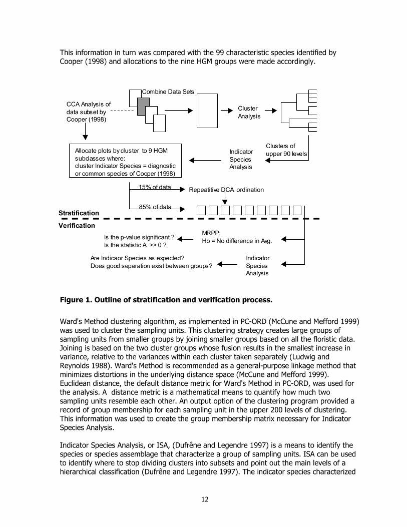
12

This information in turn was compared with the 99 characteristic species identified by Cooper (1998) and allocations to the nine HGM groups were made accordingly.

Figure 1. Outline of stratification and verification process.

Ward's Method clustering algorithm, as implemented in PC-ORD (McCune and Mefford 1999) was used to cluster the sampling units. This clustering strategy creates large groups of sampling units from smaller groups by joining smaller groups based on all the floristic data. Joining is based on the two cluster groups whose fusion results in the smallest increase in variance, relative to the variances within each cluster taken separately (Ludwig and Reynolds 1988). Ward's Method is recommended as a general-purpose linkage method that minimizes distortions in the underlying distance space (McCune and Mefford 1999). Euclidean distance, the default distance metric for Ward's Method in PC-ORD, was used for the analysis. A distance metric is a mathematical means to quantify how much two sampling units resemble each other. An output option of the clustering program provided a record of group membership for each sampling unit in the upper 200 levels of clustering. This information was used to create the group membership matrix necessary for Indicator Species Analysis. Indicator Species Analysis, or ISA, (Dufrêne and Legendre 1997) is a means to identify the species or species assemblage that characterize a group of sampling units. ISA can be used to identify where to stop dividing clusters into subsets and point out the main levels of a hierarchical classification (Dufrêne and Legendre 1997). The indicator species characterized

Combine Data Sets

Cluster Analysis

Clusters of upper 90 levels Indicator

Species Analysis

Allocate plots by cluster to 9 HGM subclasses where: cluster Indicator Species = diagnostic or common species of Cooper (1998)

Repeatitive DCA ordination

Stratification

Verification MRPP: Ho = No difference in Avg. Is the p-value significant ?

Is the statistic A >> 0 ?

Indicator Species Analysis

Are Indicaor Species as expected? Does good separation exist between groups?

CCA Analysis of data subset by Cooper (1998)

85% of data

15% of data

13

groups of sampling units and provided the relational attribute needed to allocate cluster groups to HGM subclasses. ISA provides superior results to "pruning" a dendrogram at any particular clustering level because the importance of species having large or narrow niche breadths is usually expressed at different levels of a cluster hierarchy (Dufrêne and Legendre 1997). Performing ISA on successive levels of the clustering result helped interpret the taxonomic hierarchy and provided some criteria for segregating the cluster structure. ISA was performed using PC-ORD (McCune and Mefford 1999). The analysis included the calculation of an Indicator Value (IV), identification of the group having the maximum IV, and a Monte Carlo test of the statistical significance of the maximum IV for each species. The Monte Carlo test evaluates the statistical significance of a specie's maximum IV with 250 permutations of randomized data. The probability of a Type 1 error in the permutation test is the proportion of times that the max IV from randomized data equals or exceeds the max IV from the actual data (McCune and Mefford 1999). A species Indicator Value for a group is a combined expression of the species relative abundance and relative frequency of occurrence, compared with the other groups. The index ranges from 0 to 100 and is maximum when all individuals of a species are found in a single group of sampling units and when the species occurs in all the sampling units of that group (Dufrêne and Legendre 1997). A threshold IV of 25% was used by Dufrêne and Legendre (1997) in their analyses of a carabid beetles data set. With regard to HGM subclasses, this supposes that a species having an IV of 25 % is present in at least 50% of the sampling units in one subclass and its relative abundance in that subclass (average percent cover) is 50% or greater. ISA was conducted on all clusters for each of the upper 90 levels of the cluster analysis. Species having an IV of 25% or greater and a p-value of 0.05 or less were retained. Mass assignments of sampling units to HGM subclasses were based on the results of ISA. Assignments were made by comparing (visually matching species names) the Indicator Species of a group at a given cluster level with the HGM subclass diagnostic and common species identified by CCA analysis in Cooper (1998). Outliers were inspected in each HGM subclass after the sampling units were allocated because of the extreme influence outliers may have on multivariate analyses. Outliers are not necessarily poor data, such as sampling units crossing ecotones (non-homogenous vegetation). Sampling units from semiaquatic communities (e.g. dominated by Nuphar luteum and some Potamogeton and Sparganium species) or regionally isolated, monocultural species (Carex vesicaria) were also outliers . Some outliers were permanently removed (poor sampling units) and others were temporarily removed (unusual communities) from the data. Outlier analysis was conducted using the Outlier Analysis routine of PC-ORD. Outliers were defined as greater than two standard deviations from the group mean (chi-square) distance. The location and influence of the outliers were inspected with Detrended Correspondence Analysis, or DCA ordination (Hill and Gauch Jr. 1980) using PC-ORD. The stand composition of each outlier, or group of outliers, was evaluated by querying the relational database. Then a decision was made to leave the sampling unit(s), move the sampling unit(s) to a different HGM subclass, or remove the sampling unit(s) from the data set.

14

Verification - was the stratification effective? Two procedures were used to evaluate the effectiveness of stratifying the sampling units. A non-parametric comparison test (Multi-response Permutation Procedure) evaluated how much within group heterogeneity (of the subclasses) deviated from that expected by chance. Secondly, Indicator Species Analysis was reapplied to the sampling units, now grouped by nine HGM subclasses. This was done to determine whether the new set of Indicator Species made sense from ecological and hydrogeomorphic points of view, had good separation between groups, and compared well with the characteristic species that Cooper (1998) identified. The Multi-response Permutation Procedure was run with ranked transformed Sorensen distances using the MRPP routine of PC-ORD (McCune and Mefford 1999). MRPP detects concentration within a priori groups, a similar purpose to the one-way analysis of variance F test, but with fewer statistical assumptions about the data (Zimmerman et al. 1985). The test was applied to the subclasses as an overall comparison, rather than as pair-wise comparisons. The test statistic is a descriptor of the within-group homogeneity of the real data compared to the amount of homogeneity expected by chance, indicating the degree of separation between the groups. The procedure also provides the A statistic, which is a more intuitive description of within homogeneity compared to the random expectation. The Sorensen distance metric was chosen for MRPP because it retains more sensitivity in heterogeneous data sets and gives less weight to outliers, compared to Euclidean distance (McCune and Mefford 1999). A rank transformation was applied to help correct the loss of sensitivity of distance measures as community heterogeneity increases (McCune and Mefford 1999). Applying the test to rank transformed distances changes the null hypothesis from "average within-group distance no smaller than expected by chance" to "no difference in average within-group rank of distances." (McCune and Mefford 1999). Indicator Species Analysis was used to evaluate the degree of separation of characteristic species between the individual HGM subclasses. Group membership was according to one of nine HGM subclasses. In some respects this provides more ecological insight than conducting pair-wise comparisons with MRPP and avoids Type I error and test power issues associated with non-independent multiple comparisons. If good separation existed between the nine groups, then a species maximum Indicator Value would be expected to be statistically significant and have a considerably higher value than in the other subclasses. Secondly, subclass Indicator Species should agree with the characteristic species of Cooper (1998).

15

Results

Stratification Phase Large data sets produce clustering dendrograms (a graphical output) that are large and complex. Communication and assimilation of so much information is a limitation of the hierarchical clustering of large data sets (Van der Maarel et al. 1987). Secondly, a subjective decision must be made to choose a meaningful number of groups from the dendrogram. Wishart's objective function, provided by the clustering program, guided the selection of clustering input for the Indicator Species Analysis. Wishart's objective function is a measure of the information lost as clustering agglomeration proceeds, where the objective is a compromise between minimizing the number of groups and maximizing the information retained (McCune and Mefford 1999). The objective function is based on the error sum of squares from the centroid of the cluster to each sampling unit in the cluster. Wishart's objective function was plotted for each level of the cluster analysis (Figure 2). The amount of information retained differed by only 10 % between the asympote of the curve (~200 groups) and where the rate of information retained drops rapidly (~90 groups). Indicator Species Analysis was applied to only the first 90 levels of the clustering, a tradeoff between maintaining floristic information and avoiding over complexity. Indicator Species Analysis was conducted on each of the upper (last) 90 levels of clustering. The output from each of the analyses was sorted by Indicator Value (IV) and secondarily by the p-value of each species. Species having an IV of 25% or greater and a p-value of 0.05 or less were retained, with the cluster level and the number of sampling units in the group. The clustering level at which a species exceeded an IV of 25%, and the clustering level where it obtained a maximum IV were recorded in a summary table, as suggested by Dufrêne and Legendre (1997). The summary result table made it much easier to interpret the clustering hierarchy and discern characteristic species having broad niches from those with narrow niches. Appendix D lists the species meeting the threshold IV criteria and their location in the upper 90 levels of clustering.

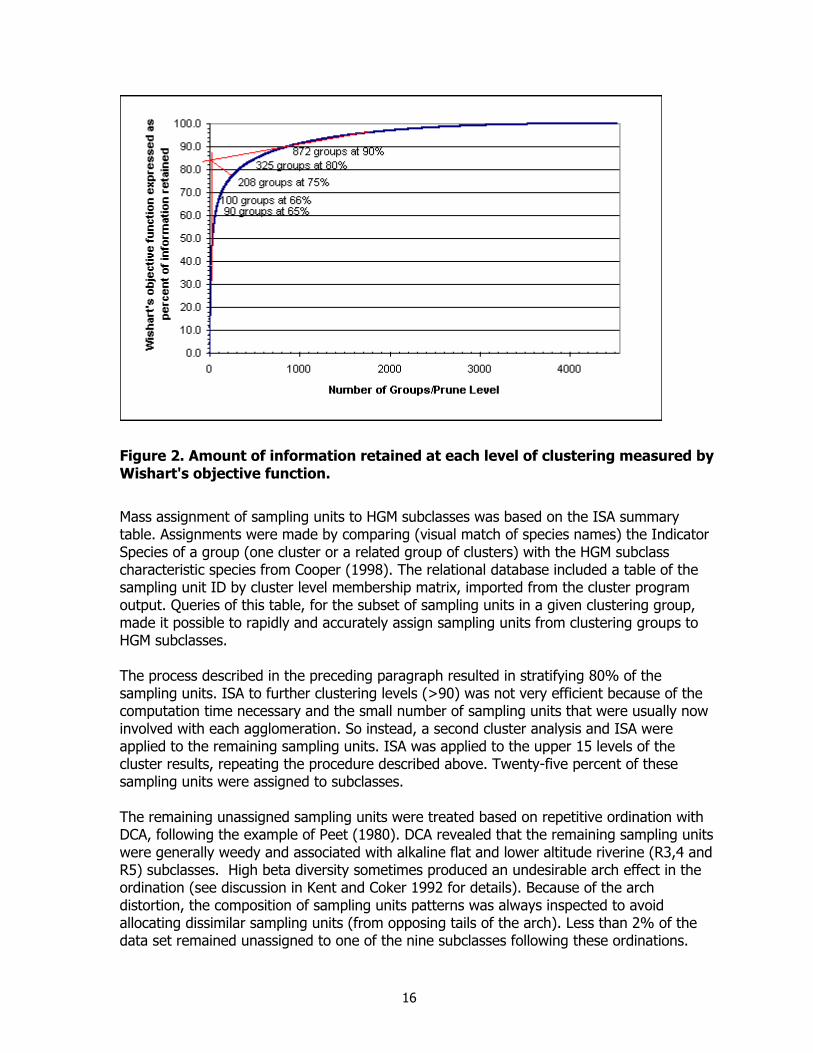
16

Figure 2. Amount of information retained at each level of clustering measured by Wishart's objective function.

Mass assignment of sampling units to HGM subclasses was based on the ISA summary table. Assignments were made by comparing (visual match of species names) the Indicator Species of a group (one cluster or a related group of clusters) with the HGM subclass characteristic species from Cooper (1998). The relational database included a table of the sampling unit ID by cluster level membership matrix, imported from the cluster program output. Queries of this table, for the subset of sampling units in a given clustering group, made it possible to rapidly and accurately assign sampling units from clustering groups to HGM subclasses. The process described in the preceding paragraph resulted in stratifying 80% of the sampling units. ISA to further clustering levels (>90) was not very efficient because of the computation time necessary and the small number of sampling units that were usually now involved with each agglomeration. So instead, a second cluster analysis and ISA were applied to the remaining sampling units. ISA was applied to the upper 15 levels of the cluster results, repeating the procedure described above. Twenty-five percent of these sampling units were assigned to subclasses. The remaining unassigned sampling units were treated based on repetitive ordination with DCA, following the example of Peet (1980). DCA revealed that the remaining sampling units were generally weedy and associated with alkaline flat and lower altitude riverine (R3,4 and R5) subclasses. High beta diversity sometimes produced an undesirable arch effect in the ordination (see discussion in Kent and Coker 1992 for details). Because of the arch distortion, the composition of sampling units patterns was always inspected to avoid allocating dissimilar sampling units (from opposing tails of the arch). Less than 2% of the data set remained unassigned to one of the nine subclasses following these ordinations.

17

Unassigned sampling units, outliers, and sampling units from semi-aquatic communities were excluded from further analyses. Overall, 4335 sampling units of the 4511 sampling units were allocated to HGM subclasses. Separate outlier analyses (chi-square and Sorensen distances) and DCA ordination was conducted on each HGM subclass as a final quality control on the stratification process. A minor amount (< 50 sampling units) of reallocations were made. These were cases where sampling units greatly influenced the ordination and were usually much more than two standard deviations from the group average distance using either distance measures.

Verification Phase The upper section of Table 2 shows the average within-group rank distance for each HGM subclass from the MRPP analysis. This statistic is a measure of the internal heterogeneity of the nine groups of sampling units (Table 2). The Depressional (1) subclass is comprised of species-poor stands dominated by Carex utriculata, this is reflected by the very low average distance for the group (Table 2). The magnitude of the Average within-group rank distances is related to the group heterogeneity, not necessarily sample size. For example, Cooper (1998) stated that the mineral soil flats subclass (Flat 1) should be subdivided when more data are available. Flat 1 is one of the smaller groups but exhibits one of the higher amounts of internal variability, supporting his observation. The MRPP test statistic was significant, indicating that at least statistically, the stratification was effective (lower section of Table 1). The null hypothesis is no difference in average within-group rank of distances. The test statistic is the difference between the observed and expected deltas divided by the square root of the variance of delta. The variance and skewness of delta describe the distribution of all possible deltas if the sampling units were randomly reallocated among the subclasses. The probability value (p-value), which is extremely less than 1%, expresses the likelihood of getting a delta as extreme or more extreme than the observed delta. McCune and Mefford (1999) point out that statistical significance (low p-value) may result when the effect magnitude (A) is small, if the sample size is large. The statistic A, or "chance-corrected within-group agreement", is a descriptor of the within-group homogeneity compared to the random expectation (McCune and Mefford 1999). In community ecology, values for A are commonly less than 0.1 and an A >0.3 is fairly high (McCune and Mefford 1999). The stratification data produced a markedly high value for A (0.4), using rank transformed distances. McCune and Mefford (1999) state: "In practice with community data, the test statistic, skewness of the test statistic under the null hypothesis, and the resulting p-value are often similar, whether the data are ranked or not. The chance-corrected within-group agreement, however, is often considerably higher after the distance measure is converted to ranks.". This was true for our data as well. Using the Sorensen distance without the rank transformation produced similar statistics, except for A, which only equaled 0.1. A regional wetland flora has high beta (between community) diversity, the rank transformation helped correct the loss of sensitivity of the distance measure due to community heterogeneity.

18

Table 2. MRPP statistics for a rank transformed Sorensen distance matrix.

HGM Subclass Avg. Ranked Distance N Depression 1 0.004 123 Riverine 1,2 0.203 775 Riverine 5 0.283 462 Slope 3,4 0.284 393 Riverine 3,4 0.311 1130 S 12 0.312 713 Flat 1 0.362 131 Depression 4,5 0.404 125 Depression 2,3 0.410 483

Test Statistic Value Test statistic: T = -1071.597 Observed delta = 0.293 Expected delta = 0.500

Variance of delta = 3.73E-08 Skewness of delta = -0.269

Chance-corrected within-group agreement, A = 0.414 Probability of a smaller or equal delta, p < 1.00E-09

Indicator Species Analysis delimited characteristic species for the nine HGM subclasses. Table 3 lists all species from the analysis that had an Indicator Value (IV) greater than twenty percent and p-values < 0.05 in a Monte Carlo test of significance of the observed maximum IV. Only species codes are shown for brevity, but the scientific name is listed below the table and Appendix B lists common names The species listed in Table 3 are ecologically explainable and their Indicator Values show good separation among the nine groups. An Indicator Value of twenty percent supposes that a characteristic species is present in at least 50% of the sampling units in one subclass and its relative abundance in that subclass (average percent cover) is 40% or greater (or vice versa). Values greater than twenty percent (rather than the twenty-five percent stratification criterion) are given to better illustrate the characteristic plant assemblages. The left section of Table 3 shows the HGM subclass and the maximum Indicator Value of each Indicator Species. The center section shows the Monte Carlo test results, based on 250 permutations with randomized data. The mean IV scores obtained from 250 calculations on randomized data provide a benchmark to compare with IV scores for the real (observed) data. The right section of the table shows the observed Indicator Values in each HGM subclass. The ISA shows there is a strong correspondence with the characteristic species that Cooper (1998) delimited, and a large difference between a species maximum IV and the IV achieved in the other subclasses.

19

Table 3. Indicator Species Analysis on HGM subclass membership. Max observed Indicator Value (IV) by HGM subclass

IV stats for randomized groups 250 permutations

Number of sampling units and observed Indicator Value for each HGM Subclass

D 1 D 2,3 D 4,5 F 1 R 1,2 R 3,4 R 5 S 1,2 S 3,4Spp ID Group Max IV Mean S.Dev p-value N= 123 483 125 131 775 1130 462 713 393CARUTR D 1 88 2.5 0.57 0.004 88 0 0 0 1 0 0 1 0ELEPAL D 2,3 41 2.3 0.61 0.004 0 41 3 0 0 0 0 0 0SCHPUN D 2,3 25 1.3 0.44 0.004 0 25 0 1 0 0 1 0 0TYPLAT D 2,3 24 1 0.37 0.004 0 24 0 0 0 0 0 0 0ECHCRU D 4,5 37 1 0.46 0.004 0 0 37 0 0 0 0 0 0XANSTR D 4,5 30 1.2 0.5 0.004 0 0 30 0 0 0 1 0 0PERLAP D 4,5 29 0.9 0.48 0.004 0 0 29 0 0 0 0 0 0POLARE D 4,5 26 0.6 0.32 0.004 0 0 26 0 0 0 0 0 0DISSTR F 1 55 1 0.38 0.004 0 0 0 55 0 0 0 0 0PUCAIR F 1 26 0.6 0.36 0.004 0 0 0 26 0 0 0 0 0SALMON R 1,2 39 2.7 0.56 0.004 0 0 0 0 39 1 0 1 0MERCIL R 1,2 39 3.3 0.64 0.004 0 0 0 0 39 3 0 3 0CALCAN R 1,2 33 3.3 0.68 0.004 0 0 0 0 33 2 0 4 0CARCOR R 1,2 32 2.9 0.64 0.004 0 0 0 0 32 1 0 4 0SALDRU R 1,2 26 1.9 0.47 0.004 0 0 0 0 26 2 0 0 0PICENG R 1,2 26 2 0.47 0.004 0 0 0 0 26 1 0 1 0DISINV R 1,2 22 2.5 0.56 0.004 0 0 0 0 22 9 0 0 0SENTRI R 1,2 22 2.5 0.65 0.004 0 0 0 0 22 1 0 6 0HERSPH R 1,2 22 2.8 0.67 0.004 0 0 0 0 22 12 0 0 0ALNINC R 3,4 37 2.7 0.55 0.004 0 0 0 0 3 37 0 0 0POPANG R 3,4 30 2.1 0.57 0.004 0 0 0 0 0 30 1 0 0ROSWOO R 3,4 30 2.7 0.61 0.004 0 0 0 0 1 30 2 0 0MAISTE R 3,4 24 2.6 0.66 0.004 0 0 0 0 5 23 0 0 0SWISER R 3,4 24 1.7 0.49 0.004 0 0 0 0 0 23 0 0 0SALEXI R 5 54 2.5 0.62 0.004 0 0 0 0 0 1 54 0 0POPDEL R 5 38 1.5 0.4 0.004 0 0 0 0 0 0 38 0 0CARAQU S 12 43 3.1 0.62 0.004 5 0 0 0 3 0 0 43 0SALPLA S 12 37 2 0.52 0.004 0 0 0 0 1 0 0 36 0PSYLEP S 12 35 2 0.52 0.004 0 0 0 0 1 0 0 35 0PEDGRO S 12 25 1.9 0.53 0.004 0 0 0 0 2 0 0 25 1CLERHO S 12 25 1.5 0.52 0.004 0 0 0 0 1 0 0 25 0JUNARC S 3,4 56 3.1 0.66 0.004 0 0 0 0 0 0 1 0 56DESCES S 3,4 23 2.7 0.68 0.004 0 0 0 0 1 0 0 9 23ARGANS S 3,4 21 1.2 0.39 0.004 0 0 0 0 0 0 0 0 21CARUTR - Carex utriculata, ELEPAL - Eleocharis palustris, SCHPUN - Schoenoplectus pungens, TYPLAT - Typha latifolia, ECHCRU - Echinochloa crus-galli, XANSTR - Xanthium strumarium, PERLAP - Polygonum lapathifolium, POLARE - Polygonum arenastrum, DISSTR - Distichlis spicata, PUCAIR - Puccinellia nuttalliana, SALMON - Salix monticola, MERCIL - Mertensia ciliata, CALCAN - Calamagrostis canadensis, CARCOR - Cardamine cordifolia, SALDRU - Salix drummondiana, PICENG - Picea engelmannii, DISINV - Lonicera involucrata, SENTRI - Senecio triangularis, HERSPH - Heracleum maximum, ALNINC - Alnus incana ssp. tenuifolia, POPANG - Populus angustifolia, ROSWOO - Rosa woodsii, MAISTE - Maianthemum stellatum, SWISER - Cornus sericea ssp. sericea, SALEXI - Salix exigua, POPDEL - Populus deltoides, CARAQU - Carex aquatilis var. stans, SALPAL - Salix planifolia, PSYLEP - Caltha leptosepala ssp. leptosepala, PEDGRO - Pedicularis groenlandica, CLERHO - Rhodiola rhodanthum, JUNARC - Juncus arcticus, DESCES - Deschampsia cespitosa ssp. cespitosa, ARGANS - Argentina anserina. The nine groups of sampling units reflect underlying environmental differences while the sampling units within each group reflect underlying environmental similarities. Generalizing the complexity of wetlands in Colorado was done by Cooper (1998), identifying major environmental gradients and delimiting preliminary hydrogeomorphic subclasses. Stratifying the data according to these underlying hydrogeomorphic and climatic gradients was a necessary second step in the community analysis of the regional wetland flora. Current

20

ecological distance metrics, used by ordination and clustering techniques, fail to adequately measure the true separation of sampling units located at opposite ends of a gradient (Ludwig and Reynolds 1988, p. 273). Stratification decreases the within group heterogeneity and partitions the underlying environmental gradient(s) into smaller units. Classification can proceed independently on each hydrogeomorphic subclass. Also, summary statistics can be generated from the sampling units by subclass. For example, statistics concerning elevation ranges or point intersect attributes from GIS. Figure 3 shows the location of the sampling units, coded by HGM subclass affiliation, that will be used in the wetland community classification.

Figure 3. Map of Colorado with sampling unit locations delimited by HGM subclass.

21

Section 2: South Park Riparian Mapping Pilot

Prepared by: Denise Culver, CNHP

James F. Ward, James F. Ward & Associates Seth McClean, CDOW Dave Lovell, CDOW

Francie Pusateri, CDOW Dawn Brownne, CDOW Alex Chappell, CDOW

June 2000

Colorado Natural Heritage Program

College of Natural Resources Colorado State University

22

Abstract In collaboration with the Colorado Department of Natural Resources Division of Wildlife (DOW) Riparian Mapping Project, the Colorado Natural Heritage Program (CNHP) initiated a pilot project in South Park (Park County), Colorado. The focus of the South Park Project was to comprehensively map riparian vegetation using the methodologies developed by the DOW and merge that data with site specific information gathered and developed by CNHP. The main objectives were to cross reference CNHP’s Statewide Wetlands Classification (SWC) with the DOW’s Riparian Mapping Units. James F. Ward & Associates were subcontracted to photo interpret and digitize the riparian vegetation for 24 topographic quadrangle maps (approximately 519,300 acres). CNHP assisted with ground-truthing the delineations and DOW post-processed the digital maps. The South Park Project as part of the Comprehensive Statewide Wetlands Classification and Characterization (CSWCC) reflects a true interagency, cooperative effort that recognizes the importance of classifying, mapping, protecting, and managing unique riparian habitats. Additionally, this project provides a necessary tool to resource managers, consultants, scientists, and members of the general public to assist in the management of riparian wetlands.

Riparian Mapping Project Background and History

The following is a summary from DOW's Riparian web page: http://ndis.nrel.colostate.edu/ndis/riparian/riparian.htm. The DOW has been involved with mapping riparian vegetation since 1990. Initially, it started out as a cooperative project with the Pike/San Isabel National Forest and Comanche/ Cimarron National Grasslands in southern Colorado. At the time, the U.S. Forest Service had the funding and the desire to map riparian vegetation but lacked a Geographic Information System (GIS) necessary to digitally process the information. The DOW lacked the funding but also had the desire and the GIS expertise as well. As a result, an interagency cooperative project was developed that mapped approximately 200 USGS quadrangle maps over a six year period from 1990-1996. The only limitation of this project, due to the source of the funding, was that the delineation ended at the Forest Service's administrative boundary. Throughout this entire process, photo interpretation of the infrared aerial photography and delineation of riparian vegetation has been done by James F. Ward & Associates. James Ward has over 25 years of photo interpretive experience primarily dealing with natural resource mapping and more specifically riparian/wetland mapping. The importance of having the same photo interpreter over the years cannot be overstated. Interpretation of riparian vegetation using aerial photographs is as much an art as a science. In order to achieve a consistent product it is important to have both a consistent methodology and consistency in interpretation. Initially, the riparian vegetation information delineated by James F. Ward & Associates was hand digitized using a sensitized digitizing tablet and mouse. This process was cumbersome and each quad took between 2 - 4 weeks of effort to process digitally. Beginning in 1993,

23

the DOW, in cooperation with the Geography Department at the University of Colorado at Colorado Springs (UCCS), experimented with mechanical scanning and digital editing and attributing of the riparian quads. This proved to be a success with comparative spatial accuracy and decreased processing time. This process has been further refined and automated over the years, and processing a single quad can now be accomplished in less than one day. Over the years, funding has been tenuous at best. Once the effort with the Pike/San Isabel National Forest was complete the DOW partnered with the Bureau of Land Management (BLM) to complete the riparian delineation on numerous USGS quadrangle maps in the Upper Arkansas River Basin. This effort, which took place in 1995, resulted in a comprehensive set of riparian vegetation maps for the Arkansas River from its headwaters to Pueblo Reservoir located just west of Pueblo, Colorado. On USGS Quads where the riparian vegetation had already been mapped on the U.S. Forest Service lands, the delineation was extended to the non-USFS lands below the USFS administrative boundary. Additionally, the classification scheme was refined and USFS and the non-USFS data merged to produce a seamless product for use by all three agencies. In 1996, a private land trust organization, The San Isabel Foundation, entered into agreement with the DOW to map riparian vegetation in Custer County, Colorado. This project was located in the Wet Mountain Valley southwest of Pueblo, between the Sangre de Cristo Mountains on the west and the Wet Mountains on the east. Again, the USFS had already mapped riparian vegetation on USFS administrative lands as part of the USFS/CDOW cooperative project. This project involved continuing that delineation below the USFS boundary onto non-USFS lands and completing a comprehensive riparian vegetation data layer for use in land use and open space planning. The San Isabel Foundation successfully applied to Great Outdoors Colorado (GOCO) for funding and the DOW provided technical and GIS expertise. In 1996, the DOW also submitted a comprehensive funding proposal to Great Outdoors Colorado to support critical wildlife data acquisition and to create a web site to consolidate the data and make it more readily available to the general public. As a result, the Natural Diversity Information Source (NDIS) was created. The GOCO funding provided support necessary to create and administer the web site and support for the acquisition of data the DOW felt was important for more efficient and effective management of Colorado's wildlife resource. GOCO provided the funding necessary to hire staff and acquire information regarding species distributions in Colorado, funding to develop landscape level vegetation information using satellite imagery (Basinwide Vegetation Mapping Project), and funding to map riparian vegetation in support of the DOW's effort begun in 1990. To date, GOCO continues to fund the Colorado Riparian Vegetation Mapping Project that has resulted in the production of approximately 200 quads of data. Currently, the DOW continues in its overall goal of comprehensively mapping riparian vegetation in Colorado. Several cooperative efforts with the U.S. Geologic Survey, Colorado Department of Natural Resources, and Colorado Wildlife Heritage Foundation resulted in the production of over 50 quads of riparian data along the Front Range from the Wyoming border south to Colorado Springs. Coincidental to that mapping effort, the DOW developed a Potentially Suitable Habitat map using logistic regression techniques in combination with

24

the riparian vegetation maps and Preble's Occurrence Database. These data are being used in the Preble's Meadow Jumping Mouse recovery and Habitat Conservation Planning Effort currently underway in numerous locales along the Front Range. Finally, recent interest has been expressed by Ducks Unlimited and they have funded the mapping of several Quads along the South Platte River between Fort Morgan and Greeley. Cooperatively funded efforts such as these have enhanced the Division's ability to map areas that might otherwise be delayed.

Mapping Methodology The following is a summary from DOW's Riparian web page: http://ndis.nrel.colostate.edu/ndis/riparian/riparian.htm. The DOW uses NAPP (National Aerial Photography Program) aerial infrared photographs to map riparian vegetation. These photos are flown at a height of 20,000 feet and purchased from the USGS as a 9" x 9" film positive at a nominal scale of 1:40,000. These photos are obtained in stereo to allow for 3-D viewing that aids in the mapping process. Riparian vegetation is mapped on a 7.5' Quadrangle basis at a scale of 1:24,000. Approximately ten aerial photos per quad are needed for stereo overlay. The photos are arranged on a stereo zoom transfer scope and registered to the corresponding topographic mylar for purposes of spatial accuracy. Although the maps are produced at a scale of 1:24,000 the delineation is performed at a scale of 1:12,000 which greatly increases both the spatial and classification accuracy. Combining the use of a pre-defined Classification Scheme, and while viewing the imagery in stereo to better ascertain vegetative and geomorphological structure, the photo-interpreter delineates riparian vegetation as either a polygon or line feature using a '000' rapidograph. The minimum mapping unit (MMU) is 1/2 acre and groupings this size or larger are depicted as polygons. In many cases, polygons as small as 1/10 acre have been delineated by the photo-interpreter during the course of this project. Riparian vegetation less than 80 feet in width is recorded as a line feature. A line feature must be at least 500 feet in length to be recorded. If a line feature is less than 500 feet long it is then incorporated into another riparian type. Delineation of the line and polygon features is done on a separate piece of stable-based mylar registered to the topographic mylar. Once the initial delineation is complete, the photo-interpreter makes a second pass and assigns attributes to the features, again, using the riparian classification scheme. The classification scheme makes use of a dominant/subdominant methodology for describing riparian vegetation. Unless a polygon is at least 75% homogeneous it is broken out with the dominant category listed first followed by the subdominant category. The dominant/subdominant attributes are separated by a slash ( / ). For example, RS/RH equals "riparian shrub/riparian herbaceous" with shrub being the dominant category within the mapped polygon. Annotation labels are delineated on a separate sheet of stable-based mylar from that used to delineate the riparian lines and polygons. This facilitates the scanning, editing, and digital processing of the data.

25

The delineations were then reviewed by CNHP using known occurrences of riparian plant communities located in the Biological Conservation Database (BCD) System, as well as previous field work knowledge. After the riparian vegetation is delineated and annotated it is mechanically scanned at a minimum resolution of 300 dpi. This resolution achieves optimal results for digital editing and attributing. The digital file is edited and attributed using LTDOS, LTPLUS, ARCSCAN, or a similar line tracer program. The resulting digital files, along with the original delineation, are then provided to the DOW for final digital processing into an ArcInfo Geographic Information System (GIS).

DOW Riparian Mapping Classification Scheme The following is a summary from DOW's Riparian web page: http://ndis.nrel.colostate.edu/ndis/riparian/riparian.htm. The photo interpretation of riparian vegetation is accomplished as outlined in the Methodology Section using the classification scheme outlined below. Potential riparian habitats are not delineated. Mixed communities are delineated when obvious spectral differences in vegetation can be discerned within a common area. For each of the classes (Table 4), a single label indicates that the class is dominant and comprises at least 75% or more of the vegetation. Other vegetation may be present but less than the Minimum Mapping Unit (MMU) of 1/2 acre. Mixed communities consists of classes that are less than 75% cover with a lesser amount of one or more other groups. The dominant type is annotated first with the lesser type following. For example, if a polygon is attributed as RT1/RS1, the vegetation in the area is less than 75% dominant of any particular class but is a mixed community of Aspen and Willow with Aspen dominant between the two classes. A forward slash ( / ) is used to separate the dominant/subdominant classes both on the hard copy and within the digital data.

Table 4. DOW Riparian Mapping Classification.

CATEGORY MAP CODE RIPARIAN DECIDUOUS TREES Riparian Deciduous Tree-General RT Riparian Deciduous Tree-Aspen RT1 Riparian Deciduous Tree-Cottonwood RT2 Riparian Deciduous Tree—Russian Olive RT3 Riparian Deciduous Tree-Birch RT4 Riparian Deciduous Tree-Boxelder RT5 Riparian Deciduous Tree-Green Ash RT6 Riparian Deciduous Tree-Mulberry RT7 RIPARIAN EVERGREEN Riparian Evergreen Tree-General RE Riparian Evergreen Tree-Blue Spruce RE1 Riparian Evergreen Tree-Engleman Spruce RE2 Riparian Evergreen Tree-Douglas Fir RE3 Riparian Evergreen Tree—Lodgepole Pine RE4

26

CATEGORY MAP CODE Riparian Evergreen Tree-Spruce/Fir RE5 Riparian Evergreen Tree-Ponderosa Pine RE6 Riparian Evergreen Tree-Cedar/Juniper RE7 Riparian Evergreen Tree-Pinon/Juniper RE8 RIPARIAN SHRUBS Riparian Shrub-General RS Riparian Shrub-Willow RS1 Riparian Shrub-Tamarisk RS2 Riparian Shrub-Alpine Willow RS3 Riparian Shrub-Gambel Oak RS4 Riparian Shrub-Sagebrush RS5 RIPARIAN HERBACEOUS Riparian Herbaceous-General RH Riparian Herbaceous-Cattails/Sedges/Rushes (with permanent standing water

RH1

Riparian Herbaceous-Sedges/Rushes/Mesic Grasses (Waterlogged or Moist Soils)

RH2

WATER BODIES Open Water-Standing OW1 Open Water-Riverine OW2 Open Water-Canal OW3 OTHER RIPARIAN Unvegetated NV Sandbar SB NON-RIPARIAN Upland Tree UT Upland Shrub US Upland Grass UG Both polygon features and line features are mapped using this classification scheme, infrared aerial photographs, 7.5 minute topographic ortho-photos, and a minimum mapping unit of 0.5 acres. This classification scheme utilizes a dominant/subdominant methodology of describing riparian habitat. Unless a polygon is at least 75% homogeneous the dominant category is listed first followed by a slash ( / ) and the subdominant category.

27

Results James F. Ward & Associates delineated 30 mapping units on 24 topographic maps for South Park. The maps were completed in June 2000. CNHP will continue to cross reference and ground-truth the CSWCC with the DOW Mapping units during the 2000 field season. The preliminary results are detailed in Table 5.

Table 5. DOW Riparian Mapping Units with proposed CNHP Plant Associations and ranks.

CATEGORY MAP CODE Proposed CNHP Plant Associations

CNHP Ranks (see Table 6 )

RIPARIAN DECIDUOUS TREES Riparian Deciduous Tree-General RT Information not available Riparian Deciduous Tree-Aspen RT1 Populus tremuloides/tall

forbs Populus tremuloides/Betula occidentalis

G5/S5

G2G3/S2 Riparian Deciduous Tree-Cottonwood RT2 Populus angustifolia/Alnus

incana Populus angustifolia/Salix exigua

G3S3?

G4/S4

Riparian Deciduous Tree—Russian Olive

RT3 Not applicable

Riparian Deciduous Tree-Birch RT4 Betula glandulosa/mesic forb-mesic graminoid Betula occidentalis/mesic forb

G3G4/S3

G3/S2

Riparian Deciduous Tree-Boxelder RT5 Not applicable Riparian Deciduous Tree-Green Ash RT6 Not applicable Riparian Deciduous Tree-Mulberry RT7 Not applicable RIPARIAN EVERGREEN Riparian Evergreen Tree-General RE Abies lasiocarpa Riparian Evergreen Tree-Blue Spruce RE1 Picea pungens/Betula

occidentalis Picea pungens/Alnus incana

G2S2

G3S3 Riparian Evergreen Tree-Englemann Spruce

RE2 Information not available*

Riparian Evergreen Tree-Douglas Fir RE3 Information not available* Riparian Evergreen Tree—Lodgepole Pine

RE4 Information not available*

Riparian Evergreen Tree-Spruce/Fir RE5 Abies lasiocarpa-Picea engelmannii/Alnus incana Abies lasiocarpa-Picea engelmanii/Salix drummondiana Abies lasiocarpa/Picea engelmanii/Mertensia ciliata Abies lasiocarpa-Picea engelmanii/Carex aquatilis

G5/S5

G5/S4

G5/S5

G3S3

28

CATEGORY MAP CODE Proposed CNHP Plant Associations

CNHP Ranks (see Table 6 )

Riparian Evergreen Tree-Ponderosa Pine

RE6 Information not available*

Riparian Evergreen Tree-Cedar/Juniper

RE7 Not applicable

Riparian Evergreen Tree-Pinon/Juniper

RE8 Not applicable

RIPARIAN SHRUBS Riparian Shrub-General RS Pentaphylloides

floribunda/Deschampsia cespitosa

G4/S3S4

Riparian Shrub-Willow RS1 Salix monticola/mesic forb Salix monticola/mesic graminoid Salix exigua/mesic graminoid Salix monticola/Carex utriculata Salix drummondiana/Carex utriculata Salix eriocephala var. ligulifolia Salix monticola/Carex aquatilis

G3/S3 G3/S3

G5/S5 G3S3

GU/S3

G3/S3

Riparian Shrub-Tamarisk RS2 Not applicable Riparian Shrub-Alpine Willow RS3 Salix brachycarpa/Carex

aquatilis Salix planifolia/Caltha leptosepala Salix planifolia/Carex aquatilis Salix wolfii/Carex aquatilis

G2G3/S2S3

G4/S4

G5/S4

G5/S4 Riparian Shrub-Gambel Oak RS4 Not applicable Riparian Shrub-Sagebrush RS5 Information not available* RIPARIAN HERBACEOUS Riparian Herbaceous-General RH Riparian Herbaceous-Cattails/Sedges/Rushes (with permanent standing water)

RH1 Typha angustifolia-Typha latifolia Utricularia vulgaris

G5/S3

G3?/S1 Riparian Herbaceous-Sedges/Rushes/Mesic Grasses (Waterlogged or Moist Soils)

RH2 Kobresia simpliciuscula-Scirpus pumilus Kobresia myosuroides-Thalictrum alpinum Carex utriculata Juncus balticus

G2?/S1

G1?/S1

G5/S5 G5/S5

WATER BODIES Open Water-Standing OW1 Information not available Open Water-Riverine OW2 Information not available Open Water-Canal OW3 Information not available OTHER RIPARIAN

29

CATEGORY MAP CODE Proposed CNHP Plant Associations

CNHP Ranks (see Table 6 )

Unvegetated NV Information not available Sandbar SB Information not available NON-RIPARIAN Upland Tree UT Information not available Upland Shrub US Information not available Upland Grass UG Information not available

Table 6. Definition of Colorado Natural Heritage Imperilment Ranks.

Global imperilment ranks are based on the range-wide status of a species. State imperilment ranks are based on the status of a species in an individual state. State and Global ranks are denoted, respectively, with an "S" or a "G" followed by a character. These ranks should not be interpreted as legal designations. G/S1 Critically imperiled globally/state because of rarity (5 or fewer occurrences in the world/state;

or very few remaining individuals), or because of some factor of its biology making it especially vulnerable to extinction.

G/S2 Imperiled globally/state because of rarity (6 to 20 occurrences), or because of other factors demonstrably making it very vulnerable to extinction throughout its range.

G/S3 Vulnerable through its range or found locally in a restricted range (21 to 100 occurrences). G/S4 Apparently secure globally/state, though it might be quite rare in parts of its range, especially

at the periphery. G/S5 Demonstrably secure globally, though it may be quite rare in parts of its range, especially at

the periphery. GX Presumed extinct. G#? Indicates uncertainty about an assigned global rank. G/SU Unable to assign rank due to lack of available information. GQ Indicates uncertainty about taxonomic status. G/SH Historically known, but not verified for an extended period, usually. G#T# Trinomial rank (T) is used for subspecies or varieties. These species or subspecies are

ranked on the same criteria as G1-G5. S#B Refers to the breeding season imperilment of elements that are not permanent residents. S#N Refers to the non-breeding season imperilment of elements that are not permanent

residents. Where no consistent location can be discerned for migrants or non-breeding populations, a rank of SZN is used

SZ Migrant whose occurrences are too irregular, transitory, and/or dispersed to be reliably identified, mapped, and protected.

SA Accidental in the state. SR Reported to occur in the state, but unverified. S? Unranked. Some evidence that species may be imperiled, but awaiting formal rarity ranking. Notes: Where two numbers appear in a state or global rank (e.g., S2S3), the actual rank of the element falls between the two numbers.

30

Discussion The South Park pilot project provides a comprehensive mapping project for federal, state, and private land managers. Coupled with CNHP’s Statewide Wetland Classification, it is the necessary tool for managing and preserving South Park’s riparian wetlands. The riparian wetlands of South Park are wetland ecosystems with very high biodiversity significance. Presently, there are a total of 29 natural plant communities within the study area. Five of these are globally rare, 10 are globally uncommon, and 14 are good examples of common communities. CNHP will be performing a Countywide Inventory in Park County during 2000 and will continue to ground truth and cross reference the DOW mapping units with the Statewide Classification. The total land area that was photo interpreted and digitized was approximately 519,300 acres. Cost per acre is $.054, does not include the digitizing costs (typically $.008/acre). Costs varied depending on the location. For example large wet irrigated areas such as South Park are more time consuming and therefore more expensive than areas of small, well-defined, natural drainage systems such as the foothills. The least expensive riparian maps would be found on the plains in eastern Colorado. Other factors that effect cost are the minimum mapping size, classification system and type of photography. South Park was unique because it ranged from extremely wet on the north end to very dry on the south. The large bare areas and salt deposits along with the fens gave the site a great deal of diversity. Expansive irrigated areas some times made it difficult to distinguish between true riparian or wetland and that which is wet only because it is irrigated. Mining along the streams and other types of man-made change added to the difficulty. The South Park Riparian Mapping Project reflects a true interagency, cooperative effort that recognizes the importance of classifying, mapping, protecting, and managing riparian wetland habitats. CNHP and DOW will continue to work toward the protection and management of Colorado’s precious resource--wetlands--using the strength of partnership and collaboration.

31

Literature Cited

1. Access 97 Relational Database Ver. SR-2. Microsoft Corporation, Seattle, WA.

2. Allen, R. B. and R. K. Peet. 1990. Gradient analysis of forests of the Sangre de Cristo Range, Colorado. Canadian Journal of Botany 68: 193-201.

3. Anderson, M., P. Bourgeron, M. T Bryer, R. Crawford, L. Engelking, D. Faber-Langendoen, K. Gallyoun, K. Goodin, D. H. Grossman, S. Landall, K. Metzler, K. D. Patterson, M. Pyne, M. Reid, L. Sneddon, and A. S. Weakley. 1998. International Classification of Ecological Communities: Terrestrial Vegetation for the United States. Volume II. Arlington, VA: The Nature Conservancy.

4. Brinson, M. M. 1993. A Hydrogeomorphic Classification for Wetlands, Technical Report WRP-DE-4. U.S. Army Corps of Engineers Waterways Experimental Station, Vicksburg, MS.

5. Costanza R., R. d'Arge, R. de Groot, S. Farber, M. Grasso, B. Hannon, K. Limburg, S. Naeem, R. V. O'Neill, J. Paruelo, R. G. Raskin, P. Sutton, and M. van den Belt. 1997. The value of the world's ecosystem services and natural capital. Nature 387: 253-60.

6. Cowardin, L. M., V. Carter, F. C. Golet, and E. T. LaRoe. 1979. Classification of wetlands and deepwater habitats of the United States, U. S. Department of the Interior, Fish and Wildlife Services, Office of Biological Services, Washington D.C.

7. Daily, G. C., S. Alexander, P. R. Ehrlich, L. Goulder, J. Lubchenco, P. A. Matson, H. A. Mooney, S. Postel, S. H. Schneider, D. Tilman, and G. M. Woodwell. 1997. Ecosystem services: benefits supplied to human societies by natural ecosystems. Issues in Ecology 2 Spring.

8. Dorn, R. D. 1997. Rocky Mountain Region Willow Identification Field Guide, R2-RR-97-01. Denver, CO: USDA, US Forest Service.

9. Dufrêne, M. and P. Legendre. 1997. Species assemblages and indicator species: The need for a flexible asymmetrical approach. Ecological Monographs 67: 3: 345-66.

10. Grossman, D. H., D. Faber-Langendoen, A. S. Weakley, M. Anderson, P. Bourgeron, R. Crawford, K. Goodin, S. Landaal, K. Metzler, K. Patterson, M. Pyne, M. Reid, and L. Sneddon. 1998. International Classification of Ecological Communities: Terrestrial Vegetation of the United States. The National Vegetation Classification System: Development, Status, and Applications. Volume I ed. Arlington, VA: The Nature Conservancy.

11. Hill, M. O. and H. G. Gauch Jr. 1980. Detrended correspondence analysis: an improved ordination technique. Vegetatio 42: 47-58.

32

12. Kartesz, J. T. and R. Kartesz. 1980. A Synonymized Checklist of the Vascular Flora of the United States, Canada and Greenland. Chapel Hill, NC: University of North Carolina Press.

13. Kent, M. and P. Coker. 1992. Vegetation Description and Analysis: A Practical Approach. 1st ed. Boca Raton, FL: CRC Press, Inc.

14. Kimmins, J. P. 1997. Forest Ecology: A Foundation for Sustainable Management. Second ed. Upper Saddle River, NJ: Prentice Hall.

15. Kittel, G. M., E. VanWie, M. Damm, R. Rondeau, S. Kettler, A. McMullen, and J. Sanderson. 1999a. A Classification of Riparian Wetland Plant Associations of Colorado: User Guide to the Classification Project, Colorado Natural Heritage Program, Colorado State University, Ft. Collins, CO.

16. Kittel, G. E. VanWie M. Damm R. Rondeau S. Kettler and J. Sanderson. 1999b. A classification of riparian plant associations of the Rio Grande and Closed Basin Watersheds, Colorado. A Classification of Riparian Plant Associations of the Rio Grade and Closed Basin Watersheds, Colorado . Colorado Natural Heritage Program, Colorado State University, Ft. Collins, CO.

17. Max, T. A., J. Schreuder, J. W. Hazard, D. D. Oswald, J. Teply, and J. Alegria. 1996. The Pacific Northwest region vegetation and inventory monitoring system, U.S. Forest Service Research Paper PNW-RP-493. Pacific Northwest Research Station, Portland, OR.

18. Maybury, K. P. editor. 1999. Seeing the Forest and the Trees: Ecological classification for Conservation. Arlington, VA: The Nature Conservancy.

19. McCune, B., and M. J. Mefford. 1999. PC-ORD. Multivariate Analysis of Ecological Data, ver. 4. MjM Software Design. Gleneden Beach, OR.

20. Mueller-Dumbois, D. and H. Ellenberg. 1974. Aims and Methods of Vegetation Ecology. New York, NY: John Wiley & Sons.

21. National Research Council. 1995. Wetlands: Characteristics and Boundaries. Washington, DC: National Academy Press.

22. Noss, R. F. 1990. Indicators for monitoring biodiversity: A hierarchical approach. Conservation Biology 4: 355-64.

23. Peet, R. K. 1980. Ordination as a tool for analyzing complex data sets. Vegetatio 42: 171-74.

24. Sanderson, J. and S. Kettler. 1996. A preliminary wetland vegetation classification for a portion of Colorado's west slope, The Colorado Natural Heritage Program, Colorado State University, Fort Collins, CO.

25. ter Braak, C. J. F. 1986. Canonical Correspondence Analysis: a new eigenvector technique for multivariate direct gradient analysis. Ecology 67: 1167-79.

33

26. The Nature Conservancy. 1996. Conservation by Design: A Framework for Mission Success. Arlington, VA: The Nature Conservancy.

27. U.S.D.A. NRCS. "The PLANTS database." Web page. Available at National Plant Data Center, Baton Rouge, LA. http://plants.usda.gov/plants/index.html.

28. Van der Maarel, E., I. Espejel, and P. Moreno-Casasola. 1987. Two-step vegetation analysis based on very large data sets. Vegetatio 68: 139-43.

29. Weber, W. A. and R. C. Wittman. 1996a. Colorado Flora: Western Slope. 2nd ed. Niwot, CO: University Press of Colorado.

30. Weber, W. A., and R. C. Wittmann. 1996b. Colorado Flora: Eastern Slope. 2nd ed. Niwot, CO: University Press of Colorado.

31. Zimmerman, G. M., H. Goetz, and P. W. Mielke Jr. 1985. Use of an improved statistical method for group comparisons to study effects of prairie fire. Ecology 66: 2: 606-11.

34

Appendix A

Data Sources

Two of the data sources below are compilations from the results of other studies. Therefore, the table lists both data sources, the original sources indented below the compiled source. Not all data of Cooper 1998 was used in current analysis. For example, sampling units that did not have spatial coordinates and sampling units from Kittel's studies. The citation of data sources (below) was intentionally separated from the Literature Citation of the report to make the distinction more apparent to the reader. Source Location Cooper 1998 (n= 2376) Cooper 1986 Cross Creek valley Cooper 1987 E-470 Beltway - E of Denver Cooper 1988 Boulder Valley and Bonny Reservoir Cooper 1990 South Park Cooper 1993 Crested Butte area Cooper 1995 Telluride Mt. Village Cooper 1995 Yampa River canyon, Green River - Lodore Canyon and

Whirlpool Split Cooper 1996 High Creek Fen, South Park Cooper and Cottrell 1988 Rollinsville area Cooper and Cottrell 1989 Cherry Creek - SE Denver Cooper and Cottrell 1990 northern CO Front Range Cooper and Gilbert 1990 Telluride region Cooper and Merritt 1996 Park Range, North Park Cooper and Severn 1992 San Luis Valley Komarkova 1979 Front Range alpine McKee et al. 1995 Animas and La Plata rivers Merritt 1996 Larimer County plains Merritt 1997 Green River, Allen Bottom, Yampa River, Deer Lodge Park Kittel et al. 1999a (n= 1925) Kettler and McMullen 1996 Routt National Forest Kittel and Lederer 1993 San Miguel and Dolores river basins Kittel et al. 1993 Yampa River basin Kittel et al. 1994 Colorado River basin and White River basin Kittel et al. 1995 Gunnison River basin Kittel et al. 1996 Arkansas River basin Kittel et al. 1997 South Platte River basin Kittel et al. 1999a Lower San Juan River and North Platte River basins Kittel et al. 1999b Rio Grande and Closed basins, Rio Grande National Forest Richard et al. 1996 San Juan National Forest Sanderson and Kettler 1996 (n= 120) central Colorado West Slope Hupalo 1999 unpublisheda (n= 90) East slope alpine and plains a: Unpublished data collected in 1999 for this project, methods are documented below the data source listing.

35

Data Sources: Cooper, D.J. 1986. Ecological studies of wetland vegetation Cross Creek Valley, Holy Cross

Wilderness Area, Sawatch Range, Colorado. Holy Cross Wilderness Defense Fund, Technical Report #2.

Cooper, D.J. 1987. Wetlands, vegetation and soils along the proposed E-470 Beltway. Unpublished report for the E-470 Partnership.

Cooper, D.J. 1988. Advanced identification of wetlands in the City of Boulder Comprehensive Planning Area. City of Boulder and EPA Region 8.

Cooper, D.J. 1990. Ecological studies of wetlands in South Park, Colorado: Classification, functional analysis, rare species inventory, and the effects of removing irrigation. Unpublished report prepared for EPA Region 8 and Park County, Colorado.

Cooper, D.J. 1993. Wetlands of the Crested Butte region: Mapping, functional evaluation and hydrologic regime. Unpublished report for the Town of Crested Butte and EPA Region 8.

Cooper, D.J. 1995. An analysis of wetland impacts in the Telluride Mountain Village. Unpublished Report to the U.S. Dept. of Justice.

Cooper, D.J. 1996. Water and soil chemistry, floristics and phytosociology of the extreme rich High Creek fen, in South Park, Colorado, U.S.A. Canadian Journal of Botany 74:1801-1811.

Cooper, D. J. 1998. "Classification of Colorado's Wetlands for Use in HGM Functional Assessment: A First Approximation." Characterization and Functional Assessment of Reference Wetlands in Colorado, CO Department of Natural Resources, Colorado Geological Survey - Division of Minerals and Geology, Denver, CO 80203.

Cooper, D.J. and T. Cottrell. 1988. Wetland finding and description of wetlands State Highway 119 - Blackhawk to the Boulder County Line. Unpublished report Colorado Dept. of Transportation by Daniel, Mann, Johnson and Mendenhall, Inc.

Cooper, D.J. and T. Cottrell. 1989. An ecological characterization and functional evaluation of wetlands in the Cherry Creek basin: Cherry Creek reservoir upstream to Frantown. Unpublished report for EPA Region 8 and Park County, Colorado.

Cooper, D.J. and T. Cottrell. 1990. Classification of riparian vegetation in the northern Colorado Front Range. Unpublished report prepared for The Nature Conservancy, Boulder, Colorado.

Cooper, D.J. and D. Gilbert. 1990. An ecological characterization and functional evaluation of wetlands in the Telluride region of Colorado. Unpublished report for EPA Region 8.

Cooper, D.J. and C. Severn. 1992. Wetlands of the San Luis Valley, Colorado: An ecological study and analysis of the hydrologic regime, soil chemistry, vegetation and the potential

36

effects of a water table drawdown. Unpublished report for CDOW, USFWS and Rio Grande Water Conservation District.

Kettler, S. and A. McMullen. 1996. Routt National Forest riparian vegetation classification. Report submitted to Routt National Forest. Colorado Natural Heritage Program, Colorado State University, Ft. Collins, CO

Kittel, G.M. and N.D. Lederer. 1993. A preliminary classification of the riparian vegetation of the Yampa and San Miguel/Dolores River Basins. Report submitted to the Colorado Department of Health and the Environmental Protection Agency, Region VIII. The Nature Conservancy’s Colorado Program, Boulder, CO.

Kittel, G., R. Rondeau, N. Lederer, and D. Randolph. 1994. A classification of the riparian vegetation of the White and Colorado River Basins, Colorado. Report submitted to the Colorado Department of Natural Resources and the Environmental Protection Agency, Region VIII. Colorado Natural Heritage Program, Colorado State University, Ft. Collins, CO

Kittel, G., R. Rondeau, and S. Kettler. 1995. A classification of the riparian vegetation of the Gunnison River Basin, Colorado. Report submitted to the Colorado Department of Natural Resources and the Environmental Protection Agency, Region VIII. Colorado Natural Heritage Program, Colorado State University, Ft. Collins, CO.

Kittel, G., R.J. Rondeau, and A. McMullen. 1996. A classification of the riparian vegetation of the lower South Platte and parts of the upper Arkansas River Basins, Colorado. Report submitted to the Colorado Department of Natural Resources and the Environmental Protection Agency, Region VIII. Colorado Natural Heritage Program, Colorado State University, Ft. Collins, CO.

Kittel, G., E. VanWie, and M. Damm. 1997. A classification of the riparian vegetation of the South Platte River Basin (and part of the Republican River Basin), Colorado. Report submitted to the Colorado Department of Natural Resources and the Environmental Protection Agency, Region VIII. Colorado Natural Heritage Program, Colorado State University, Ft. Collins, CO.

Kittel, G. M., E. VanWie, M. Dam, R. Rondeau, S. Kettler, A. McMullen, and J. Sanderson. 1999a. A Classification of Riparian Wetland Plant Associations of Colorado: User Guide to the Classification Project, Colorado Natural Heritage Program, Colorado State University, Ft. Collins, Colorado 80523.

Kittel, Gwen M., Erika VanWie, Mary Damm, Renée Rondeau, Steve Kettler, and John Sanderson. 1999b. A Classification of Riparian Plant Associations of the Rio Grande and Closed Basin Watersheds, Colorado. Prepared for: The Colorado Department of Natural Resources and the Environmental Protection Agency, Region VIII Denver, Colorado. The Colorado Natural Heritage Program, Colorado State University, Ft. Collins, CO.

Komarkova, V. 1979. Alpine vegetation of the Indian Peaks Area. J. Cramer, Vaduz, Germany.

37

McKee, J.P., D.E. Salas, and K. Willie. 1995. Animas -LaPlata Project wetland / riparian vegetation communities: Classification and inventory. Technical Service Center. U.S. Bureau of Reclamation. Denver, Colorado.

Merrit, D. M. 1997. Riparian vegetation and geomorphic features on regulated and unregulated rivers: Green and Yampa, NW Colorado. Unpublished thesis, Colorado State University. Fort Collins, Colorado.

Richard, C., G. Kittel, and S. Kettler. 1996. A classification of the riparian vegetation of the San Juan National Forest. Draft 1 to be submitted to the San Juan National Forest. Colorado Natural Heritage Program, Colorado State University, Ft. Collins, CO.

Sanderson, John and Steve Kettler 1996. A Preliminary Wetland Vegetation Classification for a portion of Colorado's West Slope, CNHP Research Report No. 13. Colorado Natural Heritage Program, Colorado State University, Ft. Collins, Colorado 80523.

1999 Field Season Methods The field methodology for the 1999 field season is documented here because the sole purpose was to collect at wetlands under represented in the aggregate data set. Field data for the SWC project were collected from June through September of 1999. A total of 99 sampling units located in 67 wetlands were surveyed on the East Slope and eastern Plains. Depressions and flats were primarily sampled, and a smaller number of seeps, irrigation-induced slope and depressions, and alpine wetlands. Seventeen microsamples (0.1 m2 Daubenmire cover frames) were evenly distributed along both sides of a 50 m tape contained in homogenous stands of vegetation. The transect was located in a stratified random manner by first determining the limits of the homogenous stand and then using a randomly determined location to start the transect. The cover of herbaceous species were estimated by percent cover in each microsample and averaged. Woody vegetation was estimated by line-intercept along 50 meters. Species intercepts were tabulated as relative percent cover, summing to 100 percent. Occasionally, in small wetlands, the tape was not laid linearly, or less than 17 microsamples were sampled. Voucher specimens were collected for all but the most common plant species, always for the sedges, grasses, and Asteracea. The identification of difficult taxa were determined from vouchers at the lab. A soil pit was located in the center of the transect and a simplified soil description recorded. Soil texture and color were determined for each soil horizon to a depth of 40 cm. The depth to the water table, mottling, oxidized rhyzospheres, and gleying were noted if present. A composite soil sample was collected from a depth of 10 cm for laboratory analysis of pH and specific conductivity. Data were recorded regarding hydroperiod characteristics, disturbance factors, HGM subclass, slope, elevation, and aspect of the wetland. The location of the site was delimited in the field on a USGS topoquad and the GPS positional coordinates recorded. A site map was sketched, indicating the transect(s) location, adjoining upland habitat, and the vegetation mosaic of the wetland.

38

Appendix B Plant species referenced in the report, sorted by scientific name. SppID Scientific Name Common NEGACE Acer negundo var. interius boxelder ALNINC Alnus incana ssp. tenuifolia gray alder ARGANS Argentina anserina silverweed cinquefoil CALCAN Calamagrostis canadensis bluejoint PSYLEP Caltha leptosepala ssp. leptosepala white marsh marigold CARCOR Cardamine cordifolia heartleaf bittercress CARAQU Carex aquatilis var. stans water sedge CARNEB Carex nebrascensis Nebraska sedge CARSCO Carex scopulorum mountain sedge CARSIM Carex simulata analogue sedge CARUTR Carex utriculata Northwest Territory sedge CARVER Carex vernacula native sedge SWISER Cornus sericea ssp. sericea redosier dogwood CORCOR Corylus cornuta beaked hazelnut DESCES Deschampsia caespitosa tufted hairgrass DISSTR Distichlis spicata inland saltgrass ECHCRU Echinochloa crus-galli barnyardgrass ELEPAL Eleocharis palustris common spikerush ELEQUI Eleocharis quinqueflora fewflower spikerush GLYSTR Glyceria striata fowl mannagrass HERSPH Heracleum maximum common cowparsnip JUNARC Juncus balticus var. montanus mountain rush KOBSIM Kobresia simpliciuscula simple bog sedge DISINV Lonicera involucrata twinberry honeysuckle MAISTE Maianthemum stellatum starry false lily of the vally MERCIL Mertensia ciliata tall fringed bluebells NUPLUT Nuphar lutea ssp. polysepala Rocky Mountain pond-lily PEDGRO Pedicularis groenlandica elephanthead lousewort PICENG Picea engelmannii Engelmann spruce PICPUN Picea pungens blue spruce POLARE Polygonum arenastrum oval-leaf knotweed PERLAP Polygonum lapathifolium curlytop knotweed POPANG Populus angustifolia narrowleaf cottonwood POPDEL Populus deltoides eastern cottonwood Potamogeton spp. pondweed PUCAIR Puccinellia nuttalliana Nuttall's alkaligrass CLERHO Rhodiola rhodanthum redpod stonecrop ROSWOO Rosa woodsii Woods' rose SALAMY Salix amygdaloides peachleaf willow SALBOO Salix boothii Booth's willow SALDRU Salix drummondiana Drummond's willow SALEXI Salix exigua narrowleaf willow SALMON Salix monticola park willow

39

SppID Scientific Name Common SALPLA Salix planifolia diamondleaf willow SARVER Sarcobatus vermiculatus greasewood SCHPUN Schoenoplectus pungens common threesquare Scirpus spp. bulrush SENTRI Senecio triangularis arrowleaf ragwort Sparganium spp. bur-reed SUACAL Suaeda calceoliformis Pursh seepweed TYPLAT Typha latifolia broadleaf cattail XANSTR Xanthium strumarium rough cockleburr

40

Appendix C Listed are the ninety-nine common and diagnostic species delimited by Cooper (1998, Figure 7) for each of 15 HGM subclasses. The subclasses are defined in Table 1 of the report. SppID Scientific Name Common Name HGMAGRGIG Agrostis gigantea redtop R4ALNINC Alnus incana ssp. tenuifolia thinleaf alder R3ALOAEQ Alopecurus aequalis shortawn foxtail D2AMPNEV Scirpus nevadensis Nevada bulrush F1ARGANS Argentina anserina silverweed cinquefoil S3BECSYZ Beckmannia syzigachne American sloughgrass D3BOLMAR Schoenoplectus maritimus cosmopolitan bulrush F1BROINE Bromus inermis ssp. inermis var. inermis smooth brome R4CALCAN Calamagrostis canadensis bluejoint R1CALSTR Calamagrostis stricta slimstem reedgrass S3CARAQU Carex aquatilis var. stans water sedge S1CARCOR Cardamine cordifolia heartleaf bittercress R1CAREMO Carex emoryi Emory's sedge R5CARLAN Carex pellita woolly sedge R4CARLIM Carex limosa mud sedge D1CARNEB Carex nebrascensis Nebraska sedge S4CARNIG Carex nigricans black alpine sedge S1CARSCO Carex scopulorum mountain sedge S1CARSIM Carex simulata analogue sedge S2CARUTR Carex utriculata Northwest Territory sedge D1CHERUB Chenopodium chenopodioides low goosefoot D5CHRLIN Chrysothamnus linifolius spearleaf rabbitbrush R5CORCOR Corylus cornuta beaked hazelnut R4CRIJUB Hordeum jubatum ssp. jubatum foxtail barley R4DESCES Deschampsia caespitosa tufted hairgrass S3DISSTR Distichlis spicata inland saltgrass F1ELEANG Elaeagnus angustifolia Russian olive R5ELEOBT Eleocharis engelmannii Engelmann's spikerush D4ELEPAL Eleocharis palustris common spikerush D3ELEQUI Eleocharis quinqueflora fewflower spikerush S2ELEROS Eleocharis rostellata beaked spikerush D4EPICIL Epilobium ciliatum ssp. glandulosum fringed willowherb D2EQUARV Equisetum arvense field horsetail R3GEUMAC Geum macrophyllum var. perincisum largeleaf avens R2GLAMAR Glaux maritima sea milkwort F1GLYGRA Glyceria grandis American mannagrass D2GLYSTR Glyceria striata fowl mannagrass R1GNAULI Gnaphalium uliginosum marsh cudweed D4HERSPH Heracleum maximum common cowparsnip R2HIPVUL Hippuris vulgaris common mare's-tail D1JUNARC Juncus balticus var. montanus mountain rush S3JUNBUF Juncus bufonius toad rush D4JUNTOR Juncus torreyi Torrey's rush R4KOBMYO Kobresia myosuroides Bellardi bog sedge S2KOBSIM Kobresia simpliciuscula simple bog sedge S2LEMMIN Lemna minor common duckweed D2LOBSIP Lobelia siphilitica great blue lobelia D3

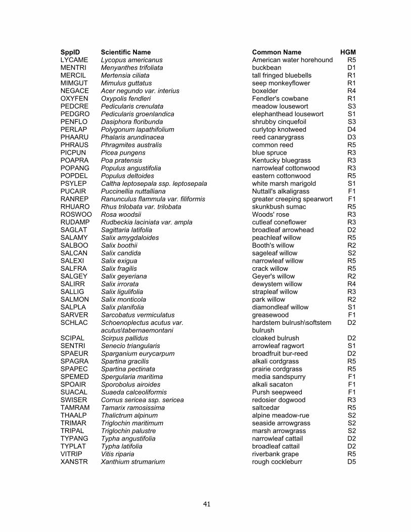
41

SppID Scientific Name Common Name HGMLYCAME Lycopus americanus American water horehound R5MENTRI Menyanthes trifoliata buckbean D1MERCIL Mertensia ciliata tall fringed bluebells R1MIMGUT Mimulus guttatus seep monkeyflower R1NEGACE Acer negundo var. interius boxelder R4OXYFEN Oxypolis fendleri Fendler's cowbane R1PEDCRE Pedicularis crenulata meadow lousewort S3PEDGRO Pedicularis groenlandica elephanthead lousewort S1PENFLO Dasiphora floribunda shrubby cinquefoil S3PERLAP Polygonum lapathifolium curlytop knotweed D4PHAARU Phalaris arundinacea reed canarygrass D3PHRAUS Phragmites australis common reed R5PICPUN Picea pungens blue spruce R3POAPRA Poa pratensis Kentucky bluegrass R3POPANG Populus angustifolia narrowleaf cottonwood R3POPDEL Populus deltoides eastern cottonwood R5PSYLEP Caltha leptosepala ssp. leptosepala white marsh marigold S1PUCAIR Puccinellia nuttalliana Nuttall's alkaligrass F1RANREP Ranunculus flammula var. filiformis greater creeping spearwort F1RHUARO Rhus trilobata var. trilobata skunkbush sumac R5ROSWOO Rosa woodsii Woods' rose R3RUDAMP Rudbeckia laciniata var. ampla cutleaf coneflower R3SAGLAT Sagittaria latifolia broadleaf arrowhead D2SALAMY Salix amygdaloides peachleaf willow R5SALBOO Salix boothii Booth's willow R2SALCAN Salix candida sageleaf willow S2SALEXI Salix exigua narrowleaf willow R5SALFRA Salix fragilis crack willow R5SALGEY Salix geyeriana Geyer's willow R2SALIRR Salix irrorata dewystem willow R4SALLIG Salix ligulifolia strapleaf willow R3SALMON Salix monticola park willow R2SALPLA Salix planifolia diamondleaf willow S1SARVER Sarcobatus vermiculatus greasewood F1SCHLAC Schoenoplectus acutus var.

acutus\tabernaemontani hardstem bulrush\softstem bulrush

D2

SCIPAL Scirpus pallidus cloaked bulrush D2SENTRI Senecio triangularis arrowleaf ragwort S1SPAEUR Sparganium eurycarpum broadfruit bur-reed D2SPAGRA Spartina gracilis alkali cordgrass R5SPAPEC Spartina pectinata prairie cordgrass R5SPEMED Spergularia maritima media sandspurry F1SPOAIR Sporobolus airoides alkali sacaton F1SUACAL Suaeda calceoliformis Pursh seepweed F1SWISER Cornus sericea ssp. sericea redosier dogwood R3TAMRAM Tamarix ramosissima saltcedar R5THAALP Thalictrum alpinum alpine meadow-rue S2TRIMAR Triglochin maritimum seaside arrowgrass S2TRIPAL Triglochin palustre marsh arrowgrass S2TYPANG Typha angustifolia narrowleaf cattail D2TYPLAT Typha latifolia broadleaf cattail D2VITRIP Vitis riparia riverbank grape R5XANSTR Xanthium strumarium rough cockleburr D5

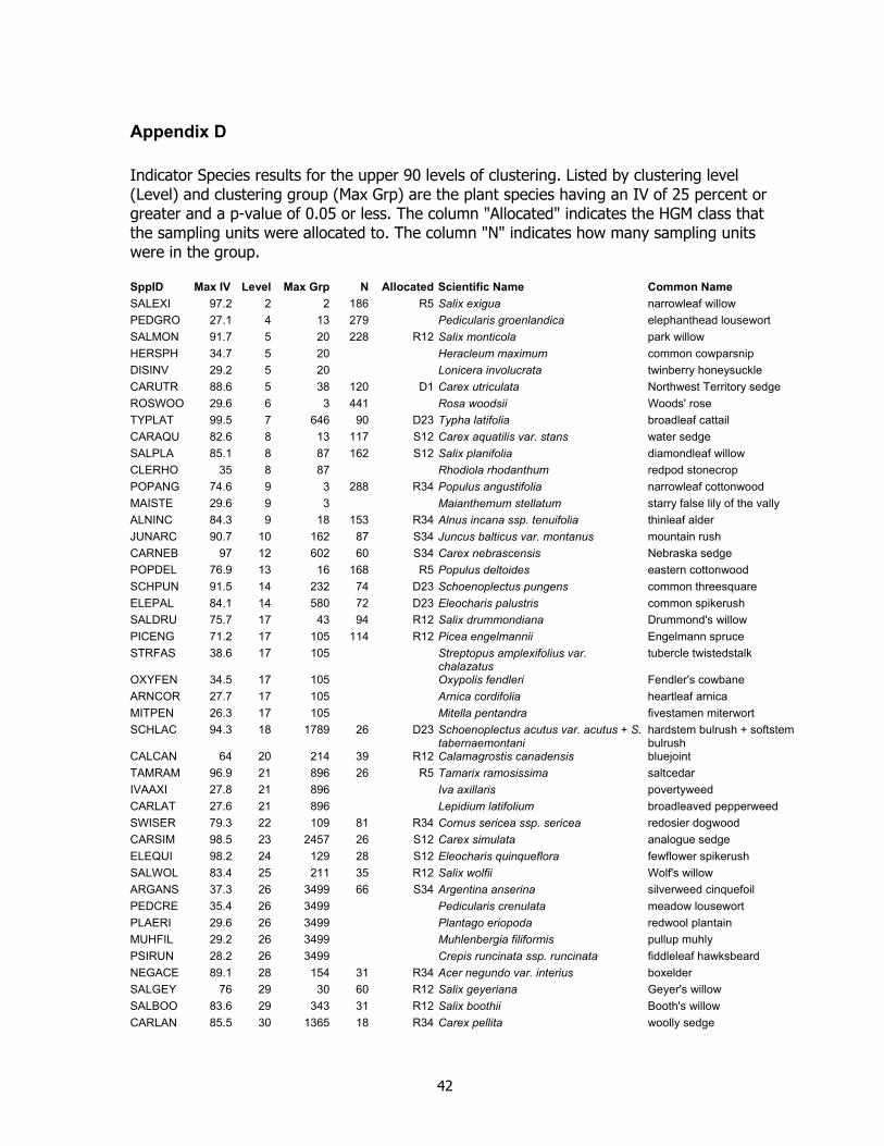
42

Appendix D Indicator Species results for the upper 90 levels of clustering. Listed by clustering level (Level) and clustering group (Max Grp) are the plant species having an IV of 25 percent or greater and a p-value of 0.05 or less. The column "Allocated" indicates the HGM class that the sampling units were allocated to. The column "N" indicates how many sampling units were in the group. SppID Max IV Level Max Grp N Allocated Scientific Name Common Name SALEXI 97.2 2 2 186 R5 Salix exigua narrowleaf willow PEDGRO 27.1 4 13 279 Pedicularis groenlandica elephanthead lousewort SALMON 91.7 5 20 228 R12 Salix monticola park willow HERSPH 34.7 5 20 Heracleum maximum common cowparsnip DISINV 29.2 5 20 Lonicera involucrata twinberry honeysuckle CARUTR 88.6 5 38 120 D1 Carex utriculata Northwest Territory sedge ROSWOO 29.6 6 3 441 Rosa woodsii Woods' rose TYPLAT 99.5 7 646 90 D23 Typha latifolia broadleaf cattail CARAQU 82.6 8 13 117 S12 Carex aquatilis var. stans water sedge SALPLA 85.1 8 87 162 S12 Salix planifolia diamondleaf willow CLERHO 35 8 87 Rhodiola rhodanthum redpod stonecrop POPANG 74.6 9 3 288 R34 Populus angustifolia narrowleaf cottonwood MAISTE 29.6 9 3 Maianthemum stellatum starry false lily of the vally ALNINC 84.3 9 18 153 R34 Alnus incana ssp. tenuifolia thinleaf alder JUNARC 90.7 10 162 87 S34 Juncus balticus var. montanus mountain rush CARNEB 97 12 602 60 S34 Carex nebrascensis Nebraska sedge POPDEL 76.9 13 16 168 R5 Populus deltoides eastern cottonwood SCHPUN 91.5 14 232 74 D23 Schoenoplectus pungens common threesquare ELEPAL 84.1 14 580 72 D23 Eleocharis palustris common spikerush SALDRU 75.7 17 43 94 R12 Salix drummondiana Drummond's willow PICENG 71.2 17 105 114 R12 Picea engelmannii Engelmann spruce STRFAS 38.6 17 105 Streptopus amplexifolius var.

chalazatus tubercle twistedstalk

OXYFEN 34.5 17 105 Oxypolis fendleri Fendler's cowbane ARNCOR 27.7 17 105 Arnica cordifolia heartleaf arnica MITPEN 26.3 17 105 Mitella pentandra fivestamen miterwort SCHLAC 94.3 18 1789 26 D23 Schoenoplectus acutus var. acutus + S.

tabernaemontani hardstem bulrush + softstem bulrush

CALCAN 64 20 214 39 R12 Calamagrostis canadensis bluejoint TAMRAM 96.9 21 896 26 R5 Tamarix ramosissima saltcedar IVAAXI 27.8 21 896 Iva axillaris povertyweed CARLAT 27.6 21 896 Lepidium latifolium broadleaved pepperweed SWISER 79.3 22 109 81 R34 Cornus sericea ssp. sericea redosier dogwood CARSIM 98.5 23 2457 26 S12 Carex simulata analogue sedge ELEQUI 98.2 24 129 28 S12 Eleocharis quinqueflora fewflower spikerush SALWOL 83.4 25 211 35 R12 Salix wolfii Wolf's willow ARGANS 37.3 26 3499 66 S34 Argentina anserina silverweed cinquefoil PEDCRE 35.4 26 3499 Pedicularis crenulata meadow lousewort PLAERI 29.6 26 3499 Plantago eriopoda redwool plantain MUHFIL 29.2 26 3499 Muhlenbergia filiformis pullup muhly PSIRUN 28.2 26 3499 Crepis runcinata ssp. runcinata fiddleleaf hawksbeard NEGACE 89.1 28 154 31 R34 Acer negundo var. interius boxelder SALGEY 76 29 30 60 R12 Salix geyeriana Geyer's willow SALBOO 83.6 29 343 31 R12 Salix boothii Booth's willow CARLAN 85.5 30 1365 18 R34 Carex pellita woolly sedge

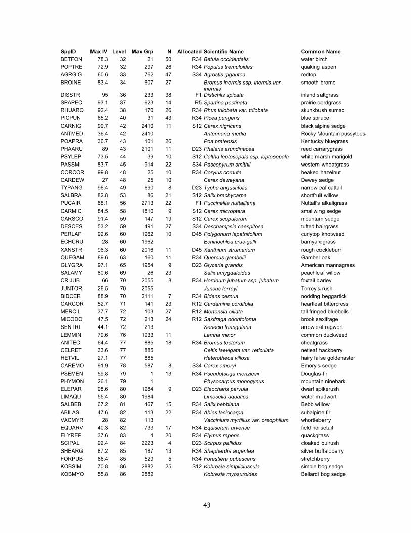
43

SppID Max IV Level Max Grp N Allocated Scientific Name Common Name BETFON 78.3 32 21 50 R34 Betula occidentalis water birch POPTRE 72.9 32 297 26 R34 Populus tremuloides quaking aspen AGRGIG 60.6 33 762 47 S34 Agrostis gigantea redtop BROINE 83.4 34 607 27 Bromus inermis ssp. inermis var.

inermis smooth brome

DISSTR 95 36 233 38 F1 Distichlis spicata inland saltgrass SPAPEC 93.1 37 623 14 R5 Spartina pectinata prairie cordgrass RHUARO 92.4 38 170 26 R34 Rhus trilobata var. trilobata skunkbush sumac PICPUN 65.2 40 31 43 R34 Picea pungens blue spruce CARNIG 99.7 42 2410 11 S12 Carex nigricans black alpine sedge ANTMED 36.4 42 2410 Antennaria media Rocky Mountain pussytoes POAPRA 36.7 43 101 26 Poa pratensis Kentucky bluegrass PHAARU 89 43 2101 11 D23 Phalaris arundinacea reed canarygrass PSYLEP 73.5 44 39 10 S12 Caltha leptosepala ssp. leptosepala white marsh marigold PASSMI 83.7 45 914 22 S34 Pascopyrum smithii western wheatgrass CORCOR 99.8 48 25 10 R34 Corylus cornuta beaked hazelnut CARDEW 27 48 25 10 Carex deweyana Dewey sedge TYPANG 96.4 49 690 8 D23 Typha angustifolia narrowleaf cattail SALBRA 82.8 53 86 21 S12 Salix brachycarpa shortfruit willow PUCAIR 88.1 56 2713 22 F1 Puccinellia nuttalliana Nuttall's alkaligrass CARMIC 84.5 58 1810 9 S12 Carex microptera smallwing sedge CARSCO 91.4 59 147 19 S12 Carex scopulorum mountain sedge DESCES 53.2 59 491 27 S34 Deschampsia caespitosa tufted hairgrass PERLAP 92.6 60 1962 10 D45 Polygonum lapathifolium curlytop knotweed ECHCRU 28 60 1962 Echinochloa crus-galli barnyardgrass XANSTR 96.3 60 2016 11 D45 Xanthium strumarium rough cockleburr QUEGAM 89.6 63 160 11 R34 Quercus gambelii Gambel oak GLYGRA 97.1 65 1954 9 D23 Glyceria grandis American mannagrass SALAMY 80.6 69 26 23 Salix amygdaloides peachleaf willow CRIJUB 66 70 2055 8 R34 Hordeum jubatum ssp. jubatum foxtail barley JUNTOR 26.5 70 2055 Juncus torreyi Torrey's rush BIDCER 88.9 70 2111 7 R34 Bidens cernua nodding beggartick CARCOR 52.7 71 141 23 R12 Cardamine cordifolia heartleaf bittercress MERCIL 37.7 72 103 27 R12 Mertensia ciliata tall fringed bluebells MICODO 47.5 72 213 24 R12 Saxifraga odontoloma brook saxifrage SENTRI 44.1 72 213 Senecio triangularis arrowleaf ragwort LEMMIN 79.6 76 1933 11 Lemna minor common duckweed ANITEC 64.4 77 885 18 R34 Bromus tectorum cheatgrass CELRET 33.6 77 885 Celtis laevigata var. reticulata netleaf hackberry HETVIL 27.1 77 885 Heterotheca villosa hairy false goldenaster CAREMO 91.9 78 587 8 S34 Carex emoryi Emory's sedge PSEMEN 59.8 79 1 13 R34 Pseudotsuga menziesii Douglas-fir PHYMON 26.1 79 1 Physocarpus monogynus mountain ninebark ELEPAR 98.6 80 1984 9 D23 Eleocharis parvula dwarf spikerush LIMAQU 55.4 80 1984 Limosella aquatica water mudwort SALBEB 67.2 81 467 15 R34 Salix bebbiana Bebb willow ABILAS 47.6 82 113 22 R34 Abies lasiocarpa subalpine fir VACMYR 28 82 113 Vaccinium myrtillus var. oreophilum whortleberry EQUARV 40.3 82 733 17 R34 Equisetum arvense field horsetail ELYREP 37.6 83 4 20 R34 Elymus repens quackgrass SCIPAL 92.4 84 2223 4 D23 Scirpus pallidus cloaked bulrush SHEARG 87.2 85 187 13 R34 Shepherdia argentea silver buffaloberry FORPUB 86.4 85 529 5 R34 Forestiera pubescens stretchberry KOBSIM 70.8 86 2882 25 S12 Kobresia simpliciuscula simple bog sedge KOBMYO 55.8 86 2882 Kobresia myosuroides Bellardi bog sedge

44

SppID Max IV Level Max Grp N Allocated Scientific Name Common Name THAALP 50.7 86 2882 Thalictrum alpinum alpine meadow-rue PTIPOR 40 86 2882 Ptilagrostis porteri Porter's false needlegrass CARCAP 29.2 86 2882 Carex capillaris hairlike sedge PARPAR 25.5 86 2882 Parnassia palustris var. parviflora smallflower grass of ParnassusSALLIG 60.6 87 35 12 R34 Salix ligulifolia strapleaf willow SALLUC 57.6 87 55 21 R34 Salix lucida ssp. caudata + ssp.

lasiandra greenleaf willow + Pacific willow

HIPHYE 79.6 88 699 9 R5 Equisetum hyemale var. affine scouringrush horsetail PENFLO 52.8 90 1189 15 S34 Dasiphora floribunda shrubby cinquefoil