Comprehensive Plan for Habitat Restoration Projects Pursuant to Reopener for Unknown Injury

1. INTRODUCTION

Presented here is a comprehensive, multi-phase plan to restore shorelines in Prince William Sound and the Gulf of Alaska affected by the Exxon Valdez Oil Spill (Comprehensive Plan). This Comprehensive Plan aims to accelerate removal of lingering subsurface oil from those shorelines by: (1) locating the remaining lingering oil, using modeling and field sampling; (2) identifying the factors that have slowed natural removal of the oil; (3) identifying and evaluating candidate bioremediation technologies and, as appropriate, alternative technologies such as tilling and physical removal; (4) pilot testing of candidate bioremediation technologies; (5) evaluating potential remediation alternatives in a draft restoration implementation plan; and (6) implementing the chosen remediation option(s). Public involvement is an important component of the Comprehensive Plan, most notably during the phases in which prioritization, of contaminated beaches for remediation, pilot testing, and evaluation of remediation options occur.

A summary of current knowledge regarding locations where lingering Exxon Valdez oil is now likely to be found and in what states of preservation appears immediately below this section. It is followed by a more detailed description of the six phases of the Comprehensive Plan. Execution of the Comprehensive Plan is explained in Section 4, where both a timeline and a decision-tree document linking the six program elements with evaluation checkpoints appear. The first two phases are expected to proceed in parallel, with the remaining phases following in sequence. A summary of cost estimates is contained in Section 5 for each of the program elements.

This Comprehensive Plan is supplemented by six appendices. Appendices A–E provide more technical detail for several of the program elements; Appendix F consists of spreadsheets detailing the estimated costs of implementing this Comprehensive Plan.

2. CURRENT STATUS OF OIL ON IMPACTED BEACHES

2.1. Geological Setting

The shorelines impacted by the oil spill in Prince William Sound (PWS) are unusual in several respects, largely because of the uplift that occurred during the 1964 Alaska earthquake. Uplift from 1.5 to 10 m raised formerly subtidal sediments into the intertidal zone. These subtidal sediments were often poorly sorted, meaning they included a wide variety of sediment sizes. Exposure to wave action after the uplift tended to transport the smaller sized particles of surface sediments either landward, forming pebble-cobble berms, or downslope toward the subtidal, where wave energy is much lower. This process leads to beach “armoring”, with larger clasts, cobbles and boulders on the surface of these beaches protecting smaller-grained sediments beneath them. Armoring stabilizes beaches by protecting the underlying sediments from reworking from wave energy and is one of the key factors contributing to the persistence of

2

subsurface oil. A similar process probably occurs in the spill zone outside PWS, where exposure to much larger waves may lead to shorelines composed of even larger particles, including large boulders, with oil trapped within the interstices.

Remediation of oil in gravel beaches and other coarse substrates poses challenges because they are highly porous, allowing deep oil penetration, and because rates of natural sediment reworking and replenishment are variable but generally slow. Armored beaches are particularly challenging, with their own unique feature combinations that have led to the persistence of oil for over 17 years:

(1) Many of the sites are sheltered from significant wave action. Even those that are relatively exposed show sediment reworking mostly in the upper intertidal zone.

(2) Many sites are not true “beaches” in the sense of sediment accumulations formed by wave action. Instead, they are rocky rubble shores – steeply sloping shores where the coarse-grained clasts consist of debris that has accumulated on the slope under the influence of gravity. These clasts show little evidence of reworking, such as sorting or rounding, or the formation of depositional berms at the high-tide line.

(3) Even the sites that are true beaches have unique characteristics. They are underlain by gently sloping surfaces of wave-carved bedrock platforms that were probably uplifted and covered by a veneer of gravel. The only truly active parts of these beaches are the high-tide and storm berms. The rest of the intertidal zone is composed of flat platforms with a stable surface armor.

(4) Most of the surface sediments are very coarse, dominated by clasts that are cobble (64-256 millimeters [mm]) and boulder (>256 mm) in size. The grain size of the gravel typically increases seaward.

2.2. Current Oil Distribution

Exxon Valdez oil has been identified at 78 distinct locations within the spill-affected region since 1998 (Fig. 1). Most of these locations were discovered during an extensive survey conducted in 2001 (Short et al. 2004), and include a variety of exposure aspects and geomorphological characteristics. Within PWS, oiled shorelines range from sheltered to very exposed. Outside PWS, oil has been found on beaches that are directly exposed to the open ocean (Irvine et al. 1999). On individual beaches, oil may be found throughout the intertidal range, although surface oil occurs most often in the upper intertidal zone, while subsurface oil is more frequent at mid-tide elevations (Fig. 2; Short et al. 2004, 2006a).

Surface oil occurs most often as weathered asphalt pavements, the thickest of which enclose softer and less weathered interiors, or as more liquid deposits of surface oil residues. The asphalt pavements are typically found on or between the cobbles and boulders that often armor beaches, whereas the surface oil residues typically contaminate the finer-grained sediments that often lay immediately beneath or between the surface armoring.

Subsurface oil is typically found as a band of oiled sediments ranging from < 1 cm in thickness to 20 cm or more, beginning a few cm below the armor if present. The transition from

3

clean sediments that overlie the oiled sediments beneath is usually very abrupt, occurring within 0.5 cm of vertical sediment depth. Most of the subsurface oil is contained within relatively few large patches, with 20% of subsurface oil patches containing 90% of the subsurface oil (Fig. 3). Most of these patches are found beneath boulder/cobble armored beaches on gently dipping slopes of the middle intertidal or within a thick sediment veneer overlying a bedrock platform (Hayes and Michel 1998, 1999, Short et al. 2004). Oil patches are occasionally found in association with other geomorphological features, such as along the bedrock margins of pocket beaches, near boulder or bedrock outcrops, or beneath mussel beds.

The subsurface oil is usually less weathered than surface oil. Especially when the concentrations of oil are high, the oil often retains a substantial proportion of the polycyclic aromatic hydrocarbons (PAH, the most toxic components of crude oil) found in the oil when spilled, as well as a complement of normal alkanes (n-alkanes, i.e. saturated hydrocarbons that have carbon atoms linked in chains; see Appendix B). Because these n-alkanes are easiest for microbes to degrade, their presence indicates that rates of microbial decomposition have been slow. The variability in the extent of weathering changes of subsurface oil indicates that local conditions or factors have important effects on microbial decomposition rates.

An estimated 56 tons of subsurface oil remained on beaches within PWS in 2001 (Short et al. 2004), but the actual amount is almost certainly greater. The estimates of lingering oil provided by the 2001 survey are limited in four ways. First, only beaches within PWS were considered, so although oil is known to persist at some locations outside PWS (Irvine et al. 1999), the extent of this contamination is not known. Second, the 2001 survey focused mainly on beaches that had been described as heavily or moderately oiled during surveys conducted from 1990 through 1992. Given the amount of oil discovered during the 2001 survey, it is almost certain that additional oil remains on other beaches that were oiled in 1989 but did not meet the selection criteria of the 2001 survey. Third, the 2001 survey only considered the upper half of the intertidal zone, and a follow-up study in 2003 (Short et al. 2006a) confirmed that the oil may often be found in the lower intertidal as well (Figure 2). Fourth, surface oil was not included in the estimates. Allowing for these sources of underestimation, the actual amount of oil remaining is probably between 100 – 200 tons (Short et al. 2004). Moreover, although substantial amounts of oil remain on some of the beaches impacted by the spill, the precise location of most of it is not known. Hence, one of the tasks of this Comprehensive Plan is to develop an efficient method for finding the bulk of the lingering oil. A probabilistic mapping approach is presented below in Section 3.1 to address this task.

4

Figure 1. Map of the spill zone showing locations of all known surface and subsurface oil deposits. Filled red circles indication locations were subsurface oil has been found since 1998 (figure continued on following page).

5

Figure 1 (continued).

0

0.1

0.2

0.3

0.4

0.5

-0.2-+0.8 0.8-1.8 1.8-2.8 2.8-3.8 3.8-4.8

tide height Interval

Freq

uenc

y

Figure 2. Frequency distributions of surface and subsurface oil with respect to tidal elevation.

6

A careful evaluation of how the larger patches of less-weathered oil are associated with shoreline oiling history and geomorphological characteristics, will provide insight into the factors promoting the preservation of oil in some patches. These factors are evaluated in Section 3.2.

0.00

0.10

0.20

0.30

0.40

0.50

0-1 1-5 5-10 10-25 25-50 50-100 100-200

>200

Oiled area (m^2)

Freu

ency

0

25

50

75

100

% a

rea

Figure 3. Frequency distribution of oiled beach sediment areas vs. patch size bins. Grey bars depict the proportion (left-hand axis) of oiled patch area within the area intervals indicated beneath them. Yellow bars depict the proportion (right-hand axis) of total oiled area associated with the area intervals indicated. Solid line connecting black diamonds shows the cumulative oiled area for the sum of the patch size intervals below and to the left.

3. RESTORATION PROGRAM ELEMENTS

The Comprehensive Plan plan consists of the following elements: (1) finding the remaining oil, (2) identifying factors limiting natural recovery, (3) evaluating removal technologies, (4) pilot testing of remediation technologies, (5) developing the final restoration plan and environmental assessment of that plan, and (6) implementation of the restoration plan.

3.1. Finding the Remaining Oil

An efficient plan for locating the remaining oil is essential because it is impractical to excavate every beach initially impacted to determine whether subsurface oil remains. Instead, a probability-based approach can locate most of the remaining oil at much lower cost. The

7

probability-based plan described below will provide a basis for assigning a probability of finding subsurface oil to each shoreline segment that was initially oiled. These assignments will then be used to prioritize selection of shorelines for remediation, beginning with shorelines where the probability of finding large patches of relatively unweathered oil is greatest, and proceeding in accordance with some stipulated criteria for minimum likely patch size and weathering state. In addition, the amounts of any oil left unremediated can be estimated and compared with the amounts subjected to treatment, and the likely locations of all the remaining oil can be mapped for consideration of remediation alternatives.

The probability-based model of oiling location and intensity will be developed iteratively, proceeding along the following six steps, which are depicted in Figure 4. This series of steps amounts to an adaptive sampling scheme, where future sampling is conditioned on information as it is acquired.

Step 1. Construct a preliminary probability model from existing information. This model has three objectives: (1) to determine whether geomorphological features can be found that are associated with lingering oil, (2) to determine the likely maximum extent of oil that would qualify for remediation efforts, and (3) to identify locations where oil is most likely to be found. This preliminary model will be based primarily on comparison of the extent of maximum oil penetration observed during the comprehensive shoreline cleanup assessment team (SCAT) surveys of the entire spill zone during fall, 1989, with shoreline geomorphology (as mapped in 2000 by NOAA using the Environmental Sensitivity Index (ESI) shoreline categories and other shoreline geomorphology data). Locations of relatively un-weathered patches of subsurface oil larger than a stipulated threshold will be added to this map, and the results examined statistically for significant associations. Most of this oil location data will be gleaned from records acquired during the 2001 and 2003 surveys of oil in PWS conducted by the Auke Bay Laboratory (ABL) (Short et al. 2004, 2006a).

Step 2. Design a statistically rigorous sampling plan to guide collection of additional field data necessary to refine the preliminary probability model. The sampling plan will address both between-beach and within-beach sampling strategies, incorporate criteria regarding minimum patch size and oil weathering state. The design of this sampling plan will be sufficiently flexible that it can be readily refined as data are acquired from other sources, including oiled locations that might be identified by the public (see Appendix A for details). A process will be established for collecting information from the public regarding locations where oil has been encountered so that this information may be used in the development of the sampling plan. See Appendix E for details regarding input from subsistence users.

Step 3. Conduct the field sampling in PWS and the northern Gulf of Alaska. The field survey objectives are to: (1) provide a statistically rigorous basis for assigning oil encounter probabilities to all shorelines oiled initially; (2) gather ancillary data for estimating the volume and surface area of the subsurface oiled sediments more accurately and precisely; and (3) gather additional data on the geomorphological characteristics associated with lingering oil, including patch sizes and oil weathering states, to refine the probability model to improve prediction of oil volumes and surface areas as well as location at a smaller spatial scale.

8

Step 4. Construct a refined probabilistic model of the spatial extent of lingering oil. The final results will include a spatial database, an assessment of the uncertainty of the predictions, and an evaluation of assumptions.

Step 5. Develop and apply criteria to prioritize beaches with lingering oil for remediation. Criteria will include the likely amount and weathering state of lingering oil present, assessment of the risks to resources and resource uses and the potential for reduction of those risks, the ability of remediation to meet restoration endpoints (based on the results of studies on the effectiveness of the tested treatment technologies; see Section 3.5), and cost estimates of the selected remediation technology (Section 3.3). Public input, is expected to play a significant role in this prioritization process. Prioritization will be based in part on data collected through the Subsistence Use, Food Safety and Risk Communication component of the plan described in Appendix E, GIS overlap maps generated from such data, and input from the work group established pursuant to that project. The risk assessment process will explicitly address uncertainties both with the remediation effectiveness and the reduction of risks to resources and resource uses. This process will provide prioritization criteria, maps and tabular data on the beaches ranked in order of remediation priority.

Step 6. During remediation, additional field data on the actual presence and distribution of lingering oil on each treated beach will be used to continually refine the model predictions and update the maps. It may be appropriate to repeat the prioritization process using the newly refined model results (Fig. 4).

9

Figure 4. Flowchart of finding lingering oil. The circled R indicates when a report would be prepared to document the results and decisions.

10

3.2 Identifying Factors Limiting Natural Recovery

Oil is removed from shorelines because of physical disturbances that disperse the oil into the adjacent water column or subtidal sediments, or because of processes in situ such as microbial degradation that either convert the oil into more mobile (polar) components or mineralize it. Physical disturbances were undoubtedly important during the years immediately following the spill. Wave action, especially during winter, could disturb surficial sediments on exposed shorelines, exposing underlying subsurface oil to more vigorous physical conditions that promote dispersive removal. Bioturbation, or the mixing of surface sediments by biota searching for prey living in near-surface sediments, is another way subsurface oil could become exposed and dispersed. Sea otters and sea stars are capable of excavating pits in the intertidal zone to depths of several tens of centimeters in search of prey, and some sea ducks and infauna such as worms can mix sediments nearer the surface. However, nearly all of the oil susceptible to loss through physical disturbance was probably removed within the first few years following the spill. Based on recent work indicating that the oiled surface area of beaches has not changed significantly since 2001 (Short et al. 2006b), it is unlikely that physical disturbance processes still play a major role in reducing oil burdens on beaches. This leaves in-situ processes as the most likely mechanisms for reducing the amount of oil remaining.

Oil stranded on shorelines provides a ready source of carbon for resident microbes, which may convert many of the oil components into carbon dioxide, water, or simpler organic compounds that are readily dispersed into the ambient air and water. The oil components most easily degraded by microbes include the aliphatic and aromatic hydrocarbons, which account for about half the mass of the oil and include the most toxic components, the polycyclic aromatic hydrocarbons (PAH). Hence, natural microbial degradation can be an effective means of detoxifying the oil by degrading the toxic PAH into simpler, less harmful products that no longer pose a contact-contamination threat to biota. Not all oil components are easily degraded by microbes, but the viscosity of the recalcitrant fraction is so high it resembles solid, friable materials that eventually become eroded into progressively finer particulates by wave action. The bioavailability of hydrocarbons in these fine organic particles is typically very low, and these particles eventually become dispersed into the adjacent water column.

The existence of highly weathered deposits of surface and subsurface oil on some of the contaminated beaches shows that microbial degradation can be effective in the spill region. This suggests that some factors, such as low temperature, which might otherwise be considered as limiting, can be discounted, and that at least at some locations, adequate nutrients were available to support microbial degradation. Identification of the factors that limit microbial degradation rates is thus crucial for evaluating whether a bioremediation strategy might be effective.

3.2.1. Candidate Factors Limiting Oil Degradation Rates

The factors most likely responsible for slow microbial degradation of subsurface oil fall into two broad categories, denoted hereafter as “nutrient limitation” and “phase boundary effects.” Nutrient limitation refers to the requirement of microbes for inorganic nutrients such as nitrogen, phosphorus, and oxygen to support their consumption of oil. Phase boundary effects refers to processes that may occur on the surfaces of oil parcels that serve to isolate the bulk of the oil from the surrounding media, be it air, water, or sediment. For example, the formation of a

11

hard outer skin on asphalt pavements slows the decomposition rate of oil beneath it, leading to some pavements that enclose less viscous and less weathered interiors. Stable emulsions, such as those occurring along Shelikof Strait, form thick deposits that are slow to weather (Irvine et al. 1999).

3.2.2. Processes Promoting Nutrient Limitation

Hydraulic stagnation refers to the likely existence of places within beaches where the flow of subsurface interstitial water, driven mainly by tidal pumping, is slow. Such stagnant water probably occurs in sediments immediately adjacent to underlying bedrock, adjacent to bedrock margins of pocket beaches, and next to boulder or bedrock outcrops. Once exhausted from such stagnant water, re-supply of oxygen and inorganic nutrients may be too slow to sustain the prolonged microbial activity needed for biophysical oil dispersion or biochemical oxidation. Hydraulic stagnation is probably an important factor because it can explain the sharp horizontal boundary often found between oiled subsurface sediments and the much cleaner sediments overlying them (Appendix B).

An inadequate supply of nutrients from the ocean, exacerbated by local depletion caused by competition from other flora such as eel grass or algae, could also retard the microbial degradation of oil. Microbial degradation rates in the environment (especially within PWS) are most likely limited by nitrogen, phosphorus, and/or oxygen (Appendix B). The ambient concentrations of nitrogen in seawater within PWS are near thresholds of limitation (Appendix B), and oxygen penetration into subsurface sediments may be sensitive to local characteristics of the sediments. A feasible mechanism through which the flux of dissolved oxygen to the lingering oil zones could be increased is addition of hydrogen peroxide (H2O2), which quickly decomposes to dissolved oxygen and water in aqueous solution. Addition of hydrogen peroxide would follow the same approach as addition of nutrients as discussed in detail in Appendix B.

3.2.3. Processes Promoting Phase-Boundary Effects

Phase-boundary effects include a wide range of processes that can limit the interactions of hydrocarbon-degrading microorganisms with the oil-water interface. Since most of the components of the lingering oil have limited solubility in water, microbial degradation requires direct contact with the oil-water interface, and anything that interferes with this contact will inhibit microbial degradation. One example of a phase-boundary effect is the formation of a “skin” that is enriched in viscous, less-degradable compounds and acts as a barrier to interphase mass transfer (Berger and Mackay, 1994), inhibiting microbial activity at the oil-water interface. Alternatively, fine sediment particles may coat the oil trapped in pores or adhere to sediment surfaces, providing a mineral barrier. Mineral fines are attracted to weathered oil by electrical charges and may provide a mechanism for natural removal of oil from coarse substrates (Bragg and Owens 1995). Water flow transports the mineral particles to the oil film; if the moving water exerts sufficient shear, the oil film can be broken into small, sediment-coated droplets, and the oil-mineral aggregates can be washed away. If the oil is too viscous or the shear force too weak, the oil cannot be desorbed and dispersed. The lingering oil may be too viscous or deep to allow formation of droplets, but the mineral particles could still be attracted to the oil-water interface and form a physical barrier that limits microbial attachment and degradation of the oil. Other processes that could block microbial interaction with the oil-water interface are also conceivable.

12

Finally, if oil is present in small, oil-filled pores, the microbial degradation rate could be limited by the areal extent of the oil-water interface.

3.2.4. Approaches to Hypothesis Testing

A better understanding of the nutrient levels (including oxygen) and the hydrodynamics of beaches that contain lingering oil will clarify the factors that limit microbial degradation. Knowing how these factors interact will facilitate selection of the most appropriate remediation technology. A field study will be conducted to determine actual oxygen and nutrient concentrations as a function of tidal cycling and to collect data (e.g., water level, temperature, salinity) to support hydrodynamic modeling of beaches in the impacted region. Hydrodynamic modeling studies, constrained by actual geomorphological characteristics (including sediment grain size distributions and variability), coupled with measurement of the subsurface transport of a conservative tracer, will be used to evaluate the likelihood of hydraulic stagnation, as well as provide a basis for adapting nutrient delivery technologies to beaches in the impacted region (see Section 3.3).

3.2.4.1. Modeling

Successful remediation will require a more detailed understanding of water flow in these beaches and the various physical processes that affect it. The three major processes are the filling and draining of the beach due to tide and waves, the physical controls on water flow in the beach imposed by beach geomorphology (i.e., profile and sediment properties), and buoyancy of the freshwater on and behind the beach. Construction of a physically-based model will facilitate evaluation of the effects of these processes and the determination of which process is dominant at a particular beach. To evaluate the fidelity of the model, two complementary approaches will be pursued. First, detailed hydraulic data from two beaches within PWS, a lentic (low energy) beach and a lotic (high energy) beach, will be obtained from a field study (Section 3.2.2.2. below and Appendix B) to calibrate the model and provide insight into the actual hydrodynamics of water flow at these beaches. Data for this model will be provided by a rigorous tracer study (Appendix B). Second, easily measured data, such as tidal level variation with time, observed values of wave runup, and large-scale beach profiles will be used to analyze the general behavior of beach hydrodynamics. This is equivalent to conducting sensitivity analyses on the beaches analyzed in the first approach.

The modeling will provide information on: (1) where the oil would most likely be located within an oiled beach, a result that could be incorporated in the statistical model of oil occurrence (Appendix A), (2) whether bioremediation is plausible from a hydraulic point of view, (3) the washout rate of nutrients from the beach, which affects the biodegradation rate of oil, and (4) where to apply the nutrients or oxygen, and at what flow rate, concentration, duration, and frequency.

3.2.4.2. Field measurements

The field study that is described in Appendix B will specifically test the hypothesis that the persistence of oil in some intertidal shorelines is due to limited transport rates for important co-substrates (e.g., nutrients and/or oxygen). Measurement of dissolved oxygen and nutrient

13

concentrations in oil-contaminated sediments will provide information that will be used to evaluate the potential for rate limitation by these substrates. Data will also be collected to validate a hydrodynamic model of solute transport in the intertidal zone, which will be used to predict the transport rates of nutrients and oxygen to the contaminated sediments under natural and enhanced (engineered) conditions. Measurements of water level and sediment permeability will provide inputs to the model, and the rate of solute transport will be measured using a conservative tracer. Comparison of the observed tracer transport to the model predictions will show whether stagnant regions exist in the subsurface sediments within the experimental domain. Once fully developed, the model will be used to determine the optimum method for applying the required amendments on beaches selected for bioremediation treatment.

Accumulation of mineral coatings at the oil-water interface will be investigated by collecting sediment samples and examining them using scanning electron microscopy.

3.2.5. Evaluation of Limiting Factors

Hydrodynamic modeling of intertidal shorelines will be used to estimate the supply rates of nutrients and oxygen to contaminated subsurface sediments, and the maximum potential rates of oil biodegradation will be estimated based on the stoichiometric requirements (see Appendix B). In addition, the pore-water concentrations of these substrates will be compared to the expected concentrations necessary to support maximum hydrocarbon biodegradation rates (e.g., 2 mg O2/L and 3-5 mg N/L). If either of these factors appears to be rate limiting, bioremediation will be implemented by providing the limiting substrates at faster rates through engineered manipulation of beach hydrodynamics. Hydrodynamic modeling, coupled with the results of the conservative tracer study, will be used to evaluate a variety of amendment application procedures and compare their expected effectiveness. The simplest and most effective procedure will be selected for pilot-scale testing.

If nutrients and/or dissolved oxygen are found to be available in sufficient quantity, some other factor must be responsible for the persistence of the lingering oil. Phase-boundary effects are likely, but more difficult to address through engineered manipulation of the shoreline hydrodynamics. Mineral barriers, if they exist, would be most difficult to overcome using nonintrusive methods. Persistence of the oil due to limited oil-water interfacial area (e.g., existence of oil-filled small pores) might be addressed by treatment of the contaminated sediments with a surfactant to mobilize the oil and increase its surface area, which would promote microbial degradation.

3.3. Evaluating Remediation Technologies

Once the factors limiting natural recovery have been identified, candidate technologies to overcome these limitations will be evaluated. Evaluation methods and criteria will be formulated, largely on the basis of modeling of water and nutrient flow in the intertidal sediments with and without candidate treatment methods. There are three steps in this program:

(1) Identify candidate technologies to overcome limiting factors

(2) Develop and apply evaluation methods and criteria for the most promising technologies

14

(3) Make the recommendation as to whether or not to proceed with pilot testing of selected technologies

The evaluation process will be similar to that used by Michel et al. (2006) in that the candidate technologies will be described and evaluated as to their potential effectiveness to remove the subsurface oil for the range of settings in PWS and the Gulf of Alaska. The results of the technology evaluation will be documented in a report describing the basis for selection of recommended technology(ies). Costs will be estimated for both a field-scale pilot test and full-scale implementation of the recommended technology(ies), based on available data for the shoreline segments selected for treatment. Although bioremediation is anticipated to be appropriate for most beaches, other treatment technologies will also be considered based on the results of the field study of limiting factors. In cases where it is determined that bioremediation methods are not effective, then other technologies, such as physical reworking and physical removal, will be evaluated. Physical removal is the likely technology for subsurface oil outside PWS where the oil often occurs as thick accumulations of stable emulsion under and between large boulders. Bioremediation is not likely to be effective on these types of oil residues. Physical reworking and removal technologies have been used in past oil spill cleanups, and their likely effectiveness and impacts are well documented. It is possible that a combination of technologies may be necessary based on site-specific conditions. If it is expected that substantial amounts of oil are likely to be left in place once this evaluation has been made, alternative means of addressing this habitat loss will be examined.

3.4. Pilot Testing of Candidate Remediation Technologies

Pilot tests of selected technologies in the field are critical to optimizing the methods and evaluating effectiveness. Field tests provide the opportunity to study processes that cannot be addressed at the smaller scale of laboratory systems or through application of simplified models. Tests will be conducted at representative sites, considering the variability among sites. Environmental conditions during the tests will be documented (e.g., temperature, storms, oil spills). The success of the selected treatment technology will be evaluated by measuring changes in the concentration and composition of the oil in treated sediments relative to untreated sediments. If necessary, the treatment methods will be refined or additional methods will be tested. A detailed description of the pilot tests focused on bioremediation technologies is provided in Appendix D. A similar approach will be used if other technologies are selected for pilot testing.

The field pilot tests will be designed to estimate the variation that exists between treated and control areas to allow evaluation of the statistical significance of any differences that are observed. A statistically valid evaluation of treatment effects will be provided by treating several independent areas and performing similar measurements on independent control areas that will not be subjected to the treatment. The criterion used to define “independence” of the treatment and control areas is that they must be clearly delineated and spatially separated. To the extent possible, treated and control areas will be set up close to one another on the same shoreline segment, such that they are similar with respect to shoreline geomorphology, wave exposure, and oil composition. Within these blocks representing similar environmental conditions, the areas that are treated and those that remain untreated will be randomly assigned. Several times during the study, samples will be collected from predetermined, randomly selected locations within each

15

block, and analysis of variance (ANOVA) will be used to evaluate the differences in oil concentration and composition over time and between treatments and controls.

The pilot test plan will also include monitoring programs to detect any potential impacts to natural and socio-economic resources. All the required permits will be obtained prior to execution of these studies, including permits from the Alaska Department of Natural Resources, Alaska Department of Environmental Conservation, U.S. Forest Service, and upland property owners. Permitting will be addressed more specifically in the study planning and scheduling.

The pilot testing will be summarized in a report that documents the test methods, results, recommendations, and costs to implement the recommended remediation technologies.

3.5. Restoration Plan and Environmental Evaluation

The decision regarding the implementation of remediation will be based on an analysis of the costs and benefits of the recommended restoration strategy, following the requirements of the National Environmental Policy Act (NEPA). An Environmental Assessment will be conducted where the proposed remediation plan will be evaluated in comparison with alternative actions including natural recovery (the “no-action” alternative) and other feasible treatment options. The proposed action and the alternatives will be described. The existing environment will be described and include selected sites both in and outside of PWS. The priority sites for restoration will have been identified, as described in Section 3.1; thus, there will be quantitative data on the number of sites and the specific areas to be restored. The environmental consequences of the proposed remediation plan and alternative actions will be assessed. This assessment will address impacts to environmental resources, socio-economic resources (including subsistence use), and cultural resources. Issues such as waste management, human health and safety, and compliance with other environmental review and permitting requirements will also be addressed.

The Draft Restoration Plan and NEPA documentation will be released for public review and comment. Public meetings will be held to solicit public input to the plan. The views of subsistence users, expressed individually and through the Subsistence Use, Food Safety and Risk Communication Project work group, will be important to the determination of remediation priorities and the propriety of using specific remediation techniques in areas where subsistence resources are located. The draft plan will be revised based on the comments received, and a Final Restoration Plan and associated NEPA documentation will be completed.

3.6 Implementation of Final Restoration Plan

The final restoration plan is likely to consist of a combination of bioremediation and physical reworking/removal technologies. The areal extent of the contaminated sediments to be treated will be based on the results of the additional field studies. For planning purposes, the estimates of the volume of oil provided by Short et al. (2004 and 2006a) and converted to estimates of the area of oiled sediments by Michel et al. (2006) are used to indicate the scope and costs. Michel et al. (Table 6; 2006) estimate that 14,369 m2 of oiled sediments described as lightly oiled residue (LOR), moderately oiled residue (MOR), and heavily oiled residue (HOR) are in the 42 segments where subsurface oil was found by Short et al. (2004). These areas represent about 12 percent of the total amount of subsurface oil in PWS based on the 2001

16

survey (Michel et al., 2006). Based on the 2003 survey data, Short et al. (2006a), estimate that there was an additional 36 percent oil in the lower intertidal zone that was not included in the oil estimates from the 2001 survey. Thus, it is estimated that there could be as much as 160,000 m2 of oiled sediments in PWS. Michel et al. (2006) estimated that 47 percent of the patches of subsurface oiled sediments were greater than 100 m2, which they used as a minimum area for treatment. However, during the environmental assessment, some sites would not be selected for remediation, because of advanced degree of weathering of the residual oil or unacceptable impacts to environmental, socio-economic, and cultural resources. It is estimated that two-thirds of the sites would be selected for remediation, estimated to cover 75,200 m2 in PWS. It is assumed that 90 percent of the selected sites in PWS with subsurface oil would be targeted for bioremediation (estimated to be 67,680 m2), and 10 percent of the sites in PWS would be targeted for physical technologies (estimated to be 7,520 m2).

Because data on sites to be remediated outside PWS are limited, this plan assumes that the area within the Gulf of Alaska selected for treatment will be approximately 13,600 m2. The Department of the Interior has identified fourteen sites outside PWS that likely contain lingering EVO. These sites are located in Kenai Fjords and Katmai National Parks, Kachemak Bay State Park, on the Pye Islands within the Alaska Maritime National Wildlife Refuge and on the Kenai Peninsula in an area where the uplands are owned by the Port Graham Corporation. The geometric mean of the areal extent of the lingering oil available for six of these sites is 340 m2. Assuming that ten of the fourteen sites would be selected for remediation in the prioritization process and that these sites represent one-fourth of the total number of sites to be remediated outside PWS, 40 sites and 13,600 m2 would be the subject of treatment outside PWS.

The restoration plan will include a program to monitor the effectiveness of the treatments and any adverse impacts. The effectiveness monitoring will be conducted after the first, second, and fourth year of treatment. The methods will be similar to those described in Brodersen et al. (1999). The effects monitoring will be conducted during implementation of the treatment methods (Appendix D). Subsistence foods sampling will be conducted after treatment. (Appendix E).

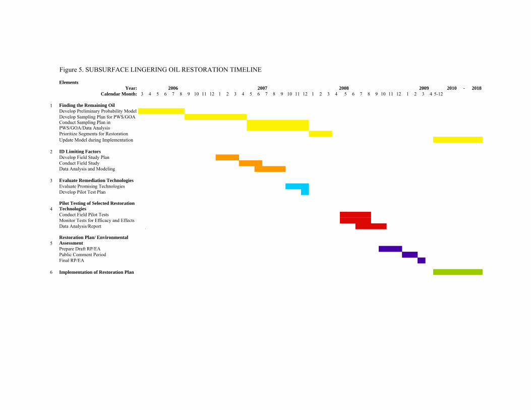
4. PLAN EXECUTION

This Comprehensive Plan will be executed through a series of phases, with decisions regarding later phases contingent on results of those completed. Figure 5 shows a proposed timeline for each program element. Comprehensive Plan execution will begin with the first two elements simultaneously: finding the lingering oil and identifying the factors that promote persistence. These two elements are not contingent on each other, so they may proceed in parallel. Similarly, the compilation of subsistence use data, pursuant to the Subsistence Use, Food Safety and Risk Communication component of the Comprehensive Plan, may also proceed in parallel. In contrast, successive Comprehensive Plan elements depend on these results, so evaluation and decision points are built into the implementation plan. This implementation plan is summarized in the two flowcharts appearing in Figures 4 (Finding the Lingering Oil) and 6 (Treatment Technology Evaluation). Implementation of the plan for finding the remaining oil is summarized in Section 3.1 above. The remainder of the implementation plan is summarized below, with reference to Figure 6.

17

Identification of the factors limiting the natural removal of the oil is the necessary first step toward treatment technology evaluation. This process begins with enumeration of the factors that contribute to oil persistence and have been summarized as hypotheses in Section 3.2.1. Tests of these hypotheses will be constructed and field programs will be designed and executed to provide data for evaluating these hypotheses (Fig. 6), and the results will be used to identify candidate remediation technologies. For example, models of groundwater flow, informed by actual measurements of the temperature, salinity, oxygen, and nutrient contents as summarized in Section 3.2.2 above, will impose restrictive constraints that lead to elimination of all but a very few limiting factors. Determining whether these potentially limiting factors are understood well enough to consider treatment options is the first major decision point of the plan for treatment technology evaluation. If these factors are not understood well enough to proceed, then new hypotheses will be formulated and methods developed to test them. For example, it may be determined that some physical reworking or removal of oiled sediments are needed under certain conditions. In the unlikely possibility that no feasible methods are identified, this Comprehensive Plan will terminate with completion of the plan for finding the lingering oil (Fig. 4). However, physical methods will always be a consideration that would be carried forward in the decisionmaking process.

If the limiting factors can be identified with sufficient confidence, the next step is to evaluate treatment options. This involves selecting treatments that are feasible given the constraints imposed by the physical environment, the level of disturbance likely to be associated with treatment, the anticipated costs, and public acceptance. If feasible treatments cannot be identified, the Comprehensive Plan would again terminate. But if feasible treatments are identified, the Comprehensive Plan will proceed to the design of specific treatment technologies, their selection and application at a pilot-scale field test as described in Sections 3.3 and 3.4 above. The efficacy of these technologies will be measured as described in Section 3.4, and compared with minimum expectations to determine whether to proceed to full-scale implementation, the next major decision of the flowchart in Figure 6. Technologies that are not adequately effective or that will have unacceptable effects on natural resources or resource uses will not be pursued, and if other candidate approaches that have not been tested are available, they will be considered for pilot-scale implementation and evaluation. If no treatment technology can be shown to be effective, the restoration plan would again terminate if no alternative means of addressing these habitat losses have been identified.

If an effective combination of treatment technologies is found, implementation will be evaluated in light of the environmental benefit, likely costs, and public input, particularly with respect to the use of specific treatment techniques in areas where subsistence resources are located. Input from the Subsistence Use, Food Safety and Risk Communication work group and individual subsistence users will be considered for this purpose. If full-scale implementation is approved, the efficacy and the impacts of implementation will be monitored. As implementation progresses, information and experience on the ground will be used to refine the means by which subsequent implementation measures are carried out and to update documentation of the locations of lingering oil.

ElementsYear: 2010 - 2018

Calendar Month: 3 4 5 6 7 8 9 10 11 12 1 2 3 4 5 6 7 8 9 10 11 12 1 2 3 4 5 6 7 8 9 10 11 12 1 2 3 4 5-12

1 Finding the Remaining OilDevelop Preliminary Probability ModelDevelop Sampling Plan for PWS/GOAConduct Sampling Plan in PWS/GOA/Data AnalysisPrioritize Segments for RestorationUpdate Model during Implementation

2 ID Limiting FactorsDevelop Field Study PlanConduct Field StudyData Analysis and Modeling

3 Evaluate Remediation TechnologiesEvaluate Promising TechnologiesDevelop Pilot Test Plan

4Pilot Testing of Selected Restoration TechnologiesConduct Field Pilot TestsMonitor Tests for Efficacy and EffectsData Analysis/Report

5Restoration Plan/ Environmental AssessmentPrepare Draft RP/EAPublic Comment PeriodFinal RP/EA

6 Implementation of Restoration Plan

2009200820072006

Figure 5. SUBSURFACE LINGERING OIL RESTORATION TIMELINE

19

Figure 6. Flowchart of remediation technology evaluation. The circled R indicates when a report would be prepared to document the results and decisions.

20

5. COST ESTIMATES (See Appendix F for details)

Finding the Remaining Oil

Preliminary Model Development: $46,325 Sampling Plan Development: $40,875 Field Sampling $1,171,750 Model Refinement: $163,500 Shoreline Prioritization: $99,735 Subtotal $1,522,185 Identification of Limiting Factors

Field Studies on Limiting Factors: $367,087 Evaluating Remediation Technologies

Identification and Evaluation of Technologies: $99,980 Pilot Testing of Candidate Remediation Technologies

Pilot Tests: $2,579,922 Final Determination on Restoration Strategy

Cost/Benefit Analysis, Final Determination: $470,935 Implementation of Final Restoration Plan

Remediation: $80,027,877 Subsistence Use, Food Safety and Risk Communication: $ 7,172,996 _______________________________________________________________ Total Costs of Comprehensive Plan $92,240,982

21

LITERATURE CITED

Berger, D. and Mackay, D. 1994. Evaporation of viscous or waxy oils – when is liquid-phase resistance significant? Proceedings, 17th Arctic and Marine Oil Spill Program (AMOP) Technical Seminar, pp. 77-92. Environment Canada, Ottawa, Ontario, Canada.

Bragg, J.R., Owens, E.H. 1995. Shoreline cleansing by interactions between oil and fine mineral

particles. Proc. International Oil Spill Conference, American Petroleum Institute Publ. No. 4620, Washington, DC, pp. 219-227.

Brodersen, C., Short, J., Holland, L., Carls, M., Pella, J., Larsen, M., Rice, S. 1999. Evaluation

of oil removal from beaches 8 years after the Exxon Valdez oil spill. Proceedings of the Twentysecond Arctic and Marine Oilspill Program (AMOP) Technical Seminar, Environment Canada, Ottawa, Ont. pp. 325-336.

Hayes, M.O., Michel, J. 1998. Evaluation of the condition of Prince William Sound shorelines

following the Exxon Valdez oil spill and subsequent shoreline treatment: 1997 geomorphological monitoring survey. Hazardous Materials Response and Assessment Division, NOAA, Seattle, Wash., 109 pp. + app.

Hayes, M.O., Michel, J. 1999. Factors determining the long-term persistence of Exxon Valdez oil

in gravel beaches: Mar. Poll. Bull., 38:92-101. Irvine, G.V., Mann, D.H., Short, J.W. 1999. Multi-year persistence of oil mousse on high

energy beaches distant from the Exxon Valdez spill origin. Mar. Pollut. Bull. 38:572-584.

Michel, J., Nixon, Z., Cotsapas, L. 2006. Evaluation of oil remediation technologies for lingering

oil from the Exxon Valdez oil spill in Prince William Sound, Alaska. Restoration Project 050778, Final Report, Exxon Valdez Trustee Council, Anchorage, AK, 47 pp + app.

Short, J.W., Lindeberg, M.R., Harris, P.M., Maselko, J.M., Pella, J.J., Rice, S.D. 2004. Estimate

of oil persisting on the beaches of Prince William Sound 12 years after the Exxon Valdez oil spill. Environ. Sci. Technol. 38:19-25.

Short, J.W., Maselko, J.M., Lindeberg, M.R., Harris, P.M., Rice, S.D. 2006a. Vertical

distribution and probability of encountering intertidal Exxon Valdez oil on shorelines of three embayments within Prince William Sound, Alaska. Environ. Sci. Technol. (in press).

Short, J.W., Irvine, G. V., Mann, D. H., Maselko, J. M., Pella, J. J., Lindeberg, M. R., Payne, J.

R., Driskell, W. B., Rice, S.D. 2006b. Slightly Weathered Exxon Valdez oil persists in Gulf of Alaska Beach Sediments after 16 years. To be submitted.

22

Wolfe, D.A., Hameedi, M.J., Galt, J.A., Watabayashi, G., Short, J., O’Clair, C., Rice, S., Michel, J., Payne, J.R., Braddock, J., Hanna, S., Sale, D. 1994. The fate of the oil spilled from the Exxon Valdez. Environ. Sci. Technol. 28 (13): 561A-568A.

23

APPENDIX A. FINDING THE REMAINING SUBSURFACE OIL A1.0 INTRODUCTION

A method for prioritizing the shorelines of Prince William Sound (PWS) and the Gulf of Alaska based upon the probability of finding lingering subsurface oil from the Exxon Valdez Oil Spill (EVOS) is critical in improving the efficiency and cost-effectiveness of any remediation effort. The potential for the development of a probability-based model of the distribution of lingering subsurface oil from the EVOS for all shorelines using field data, and any other available variables correlated with subsurface oil presence and persistence, is evaluated in this appendix. The construction of such a model will be phased. The steps involved for model development, refinement, and application will be as follows:

1) Preliminary model construction 2) Sampling plan development 3) Field sampling 4) Model refinement 5) Shoreline prioritization 6) Ongoing model refinement

This appendix outlines the proposed methodology for each of the steps in the development and application of this model. Also included are descriptions of the methods and results of a preliminary modeling effort. A2.0 METHODS OF STUDY A2.1 Preliminary Model Construction The core of the approach is the development of a statistical model relating field sampling data with other information thought to be related to the presence and persistence of subsurface oil. This model will then be used to predict the probability of finding subsurface oil at unsampled locations. Statistical predictive models may take many forms, depending upon data available and nature of the values being predicted. In the context of remediation of subsurface oil in PWS, the probability of presence, amount, status, and configuration of subsurface oil are all potentially useful in prioritizing shorelines for treatment. As such, one or more similar models that predict the selected response variables may be needed. The data generated by the extensive fieldwork carried out by NOAA’s Auke Bay Laboratory (ABL) in 2001 and 2003 (Short et al., 2004 and 2006a) would be used as field data. These data were derived from a stratified random sample of multiple beach segments in PWS. Each segment was sampled for the presence of subsurface oil by digging multiple pits. These can be evaluated as measurements of the presence, amount, status, and configuration of lingering subsurface oil – elements which form the response variables. For example, it may be possible to estimate overall subsurface oil encounter probability using the logistic family of Generalized

24

Linear Models (GLM). It may also be possible to estimate mass, volume, percent coverage, or areal extent using traditional linear models, or number of patches of oil of some significant size using Poisson family of GLM. Generalization of these models, Poisson, logistic, or otherwise, may be necessary to adequately describe the variation in the measurements and will likely involve so-called hierarchical model structure. In these types of models, multiple levels of nested unknown stochastic effects are used to represent variation at different levels of the data. Bayesian Markov-Chain Monte Carlo (MCMC) methods are used to evaluate the posterior probability distribution for the unknowns in these hierarchical models. This posterior probability distribution describes the joint uncertainty in the unknowns given the survey data, and is computed from the likelihood function of the data and a prior probability distribution of the unknowns. In the Poisson case, such an hierarchical model is very similar to that of Christiansen and Morris (1997). In most cases, predictor variables will be derived from spatially continuous proxy variable data sets constructed using Geographic Information Systems (GIS). These variables will be derived from many sources, based on knowledge of factors influencing oil deposition, persistence, and weathering on shorelines. These will include, at minimum, one or more variables from each of the following categories:

1) Shoreline geomorphology 2) Shoreline geometry 3) Backshore geomorphology 4) Oiling history 5) Nearshore oceanography

Exploratory data analysis will then be conducted, wherein all potential explanatory variables are screened for the presence of significant correlation with the response variable or variables of interest. Screening methods may include examination of data plots, significance testing of univariate linear models by Analyses of Variance (ANOVA) or Analysis of Covariance (ANCOVA), stepwise selection of significant variables in multivariate linear models, and n-fold cross validation of promising models to prevent overconfidence in their performance. Variables determined to be useful will be included in the final model. The adoption of Bayesian MCMC methods to evaluate probabilities in hierarchical models may also allow the incorporation of expert opinion and prior beliefs. A potential second stage will involve incorporation of spatial information in the model other than that captured by the explanatory variables. This would likely be accomplished by geostatistical interpolation (kriging) of model residuals from the stage-one model component. Such hybrid models are known as regression kriging, or kriging with external drift. Hengl et al. (2004) and McBratney et al. (2000) provide background on such hybrid models. Use of non-Euclidean distance metrics may be attempted, though this poses some statistical challenges (Curiero, 2005). Potentially, spatial effects not related to the predictor variables could also be incorporated using additional levels of random effects within a hierarchical model and evaluated using Bayesian MCMC methods.

25

A2.2 Sampling Plan Development The preliminary model uses field data from ABL, as well as ancillary spatially distributed data to build a spatially explicit model of probability of subsurface oiling. The data collected by ABL were collected according to a sampling plan designed to answer a specific question: how much subsurface oil remains in PWS? This question is different from the one at issue here, which is: where and in what form is subsurface oil likely to be, if present? The segments surveyed by ABL were selected according to a simple random design, or length proportional with replacement design, within six strata defined as in Table A-1. Strictly speaking, this sampling frame represents the spatial and statistical boundaries to which one may extrapolate with any model based upon these data. There is an ongoing debate as to the extent that sample design must be considered when deriving statistical models, as opposed to parameters, based on sample data (Groves 1989; Skinner et al. 1989; Korn and Graubard 1995; Hansen et al. 1983). A compromise position adopted by some is to incorporate into the model the variables that were used to define the strata, the primary sampling units, and the weights. Obviously, it is desirable to extrapolate to all shorelines affected by the EVOS, rather than those that formally lie within the scope of inference. A statistically rigorous sampling plan will be designed to guide collection of additional field data necessary to extend the spatial and statistical scope of model inference. TABLE A-1. Sampling strata from ABL 2001 study.

Strata Segment Length 1989 SCAT Descriptor

1990-1993 SCAT Descriptor

1 < 100 m Any Heavy 2 = 100m Any Heavy 3 < 100 m Any Moderate 4 = 100m Any Moderate 5 < 100 m Heavy Light or less 6 = 100m Heavy Light or less

The sampling plan will address both between-beach and within-beach sampling strategies, will incorporate criteria regarding minimum patch size and oil weathering state, and will include an assessment of the uncertainty of the results. The design of this sampling plan will be sufficiently flexible that it can be readily refined as data are acquired from other sources, including oiled locations that are identified by the public. A2.3 Field Sampling

The next step in developing the probability model will be to conduct the field sampling in PWS and the northern Gulf of Alaska. The field survey objectives would be to:

26

1) Expand the statistical scope of inference of the preliminary model or models used to predict variables related to subsurface oil persistence throughout the desired spatial extent;

2) Gather ancillary data for estimating variables related to subsurface oil persistence more accurately and precisely; and

3) Gather additional data on the fine-scale geomorphic characteristics of the lingering oil, including patch sizes and oil weathering states to improve prediction of variables related to subsurface oil persistence, as well as location at a finer spatial scale.

A2.4 Model Refinement The results of the field sampling effort described above would then be used to refine the preliminary probabilistic model of the spatial extent of lingering oil in PWS. At minimum, the additional data collected will be used to refine the parameters of the existing preliminary model. New predictive factors might be identified in the course of field sampling that would recommend inclusion in the refined model. The final results will include a spatial database, an assessment of the uncertainty of the predictions, and an evaluation of the validity of any assumptions.

A2.5 Shoreline Prioritization The results of the refined model will be used to prioritize beaches with lingering oil for remediation. Criteria will include predicted amount, configuration, and weathering state of lingering subsurface oil, assessment of the risks and potential for risk reduction to marine resources and resource uses, and the ability of remediation to meet restoration endpoints (based on the results of studies on the effectiveness of the tested treatment technologies; see Section 3.5). Public input will be an important component of this step. The results will include a report that describes the prioritization criteria and maps and tabular data on the beaches ranked in order of remediation priority. At this stage, it is expected that the results of the remediation technology evaluation (see Appendix D) will be available to finalize the costs of remediation, and to make the final determination to proceed with implementation of remediation at the priority sites. A2.6 Ongoing Model Refinement

During implementation of remediation at the priority sites, additional field data on the actual presence and distribution of lingering oil on each treated beach will be generated. These data will be used to continually refine the model predictions and update the maps. It may be appropriate to repeat the prioritization process using the newly refined model results.

27

A3.0 PRELIMINARY MODEL TEST An example statistical model has been developed after the guidelines proposed in Section A.2.1. This model serves as a proof-of-concept and initial screening of available predictor variables. A more robust, formally parameterized preliminary model will be developed prior to the development of a sampling plan as the process progresses. Figure A-1 depicts the location of input data from the 2001 ABL study in western PWS, and boundaries of study area.

FIGURE A-1. Location of shoreline segments surveyed by ABL in 2001 in western PWS. Red box represents boundary of study area. A3.1 Spatial Data Models

The construction of the model involves evaluation of response variables as collected in the field and predictor variables mainly derived from existing GIS data sets. These data are all spatially referenced, but use different spatial data models. For example, the Environmental Sensitivity Index (ESI) shoreline geomorphology data (NOAA, 2000) are spatially referenced as vector line segments representing shorelines, while the exposure index predictor variables are spatially referenced as a raster grid of rectangular 25 m x 25 m cells. In order to relate all data using a single spatial data model, all vector data were converted to raster grids, using a common 25 m cell size. This cell size is a compromise between spatial detail and computational efficiency. Analyses were carried out for all cells simultaneously. Each sampled segment was represented as one or more vector polygons describing the boundaries of that segment. These data were converted to the common spatial data model by

28

projecting the endpoints of the long axis of each polygon to the nearest point on the vector shoreline from the ESI data. The resulting vector line segments were then converted to raster grid using a 25 m cell size, as in Figure A-2. In each case, predictor variables, described below, were generated for each of 25 m cells in the raster grid representing the shoreline. These values were then evaluated within the cells representing each sampled segment from ABL. Each sampled segment is represented by between one and ten 25 m square cells, depending upon segment length and local shoreline complexity.

A. B. FIGURE A-2. (A) Vector ESI shoreline and vector polygons depicting outlines of ABL sampled segments (in red), and (B) rasterized vector shoreline and sampled segments at 25 m cell size. A3.2 Predictor Variables A3.2.1 Shoreline Geomorphology Shoreline geomorphology is known to have a strong relationship with deposition and persistence of stranded oil. Shoreline geomorphology was incorporated using categorical variable(s) derived from the ESI data set. These data consist of categorical values describing shoreline landforms or combinations of landforms attached to vector line segments. This vector line data set was converted to a raster grid with a 25 m cell size. These ESI codes were converted to a series of binary indicator variables for inclusion in the model as in Table A-2. For each sampled segment, values for the shoreline geomorphology indicator variables were generated by evaluating all ESI codes occurring in any cells representing that segment. In most cases, only a single value occurred within a given segment.

29

TABLE A-2. ESI values, descriptions and binary indicator variable values. ESI Value Description Marsh Flat Gravel Rubble Platform Rock

1A Exposed rocky shoreline 0 0 0 0 0 1 2A Rock platform 0 0 0 0 1 0 6A Gravel beach 0 0 1 0 0 0 7 Exposed tidal flat 0 1 0 0 0 0

8A Sheltered rocky shoreline 0 0 0 0 0 1 8D Sheltered rocky rubble 0 0 0 1 0 0 10A Salt marsh 1 0 0 0 0 0

A3.2.2 Shoreline Geometry Shoreline geometry, specifically convexity/concavity, is known to influence the wave and current energy incident upon a shoreline and, thus, may affect the deposition and persistence of stranded oil. Shoreline geometry was incorporated using a continuous index of concavity/convexity calculated for each 25 m cell representing shoreline. This index was calculated, for each cell, as the arithmetic mean of all cells within a given radius in a land/water raster grid wherein cells were coded as zero for water and one for land. This yielded a unitless index ranging from near zero (extremely convex) to near one (extremely concave). This index was calculated using radii of two different sizes: 100 m and 1 km. These represent convexity/concavity at two different spatial scales. For each sampled segment, an arithmetic mean of each convexity/concavity index was generated from all cells representing that segment. A3.2.3 Backshore Geomorphology

Geomorphology of the backshore, or areas adjacent to the shoreline to landward, are thought to control deposition and persistence of stranded oil in that upland topography affects both shoreline geomorphology and shallow subsurface hydrology. Though more sophisticated indices based upon topography may be used in the future (see Sorenson, 2006) backshore geomorphology was incorporated in this test preliminary model using a measure of topographic slope. Slope in degrees was calculated for each cell representing land using a digital elevation model (USDA, 1996) resampled to the common 25 m cell size. For each sampled segment, an arithmetic mean of slope in degrees was generated from all cells representing that segment and all cells adjacent to that segment to landward. A3.2.4 Oiling History Historical shoreline oiling is an obvious candidate for inclusion in the model. Historical oiling was evaluated using categorical variable(s) derived from maps of shoreline oil distribution produced by Shoreline Cleanup Assessment Team fieldwork during the fall of 1989. These data consist of descriptive oiling attributes attached to vector line segments. Because the SCAT values from 1989 were attached to a vector shoreline different from the ESI vector shoreline, attributes were transferred to the 25 m raster shoreline grid via a Euclidean allocation operation. Each 25 m cell within 100 m of the 1989 SCAT data vector shoreline was assigned the SCAT

30

code value of the nearest point on that vector line. These SCAT codes were converted to ordinal numeric codes for inclusion in the model as in Table A-3. TABLE A-3. Fall 1989 SCAT descriptors and ordinal numeric codes. Oiling Description Code No Impact 1 Very Light 2 Light 3 Medium 4 Heavy 5 For each sampled segment, an oiling history numeric code was generated by selecting the majority value from all cells representing that segment. In most cases, only a single value occurred within a given segment. A3.2.5 Nearshore Oceanography Exposure to wind and wave energy is a principle factor in controlling persistence of oil on shorelines. Shoreline exposure to wave and current energy was evaluated using raster grids of results from wind-wave fetch models and weather data. The lack of meteorological data in western PWS led to the selection of climactic summary data from NDBC data buoy 46060 (NOAA, 2006) as the best representative data set for evaluating winds in the area of interest. This data buoy is located in open water in the center of PWS, closest to the area of interest, and is not affected by local topographic effects that influence other potential data collection locations. A summary exposure index was created using methods modified from Hayes (1996). Figure A-3 shows a wind rose diagram of cumulative frequency of wind speed in knots by direction in two classes: 10 to 20 knots and greater than 20 knots. These two classes of wind speeds are critical in construction of this index. The majority of winds greater than 10 knots in velocity blow from between 90 and 120 degrees (East-Southeast). Fetch was calculated as a raster operation according to the USACE (1984) modified effective fetch calculation methodology. This method calculates fetch in a given direction as the arithmetic mean of the over-water length of 9 radials around that direction at 3-degree increments. Inputs to the operation consisted of a land-water grid with a 25 m cell size, wherein fetch length is calculated for each open water grid cell. Exposure index is then calculated for each open water cell as such:

∑=

+=12

1

2 )]10*[*(])10*[*(i

iiii PsFPFEI

where EI is a unitless index of wave exposure, i is the wind direction, Fi is modified effective fetch as calculated in direction i in kilometers, Pi is the cumulative percentage of time the wind blows between 10 and 20 knots from direction i, and Psi is the cumulative percentage of time the wind blows at greater 20 knots from direction i. Figure A-4 depicts the results of this analysis.

31

0

5

10

15350 -010

020-040

050-070

080-100

110-130

140-160

170-190

200-220

230-250

260-280

290-310

320-340

> 20 kts

10 - 20 kts

FIGURE A-3. Polar plot of cumulative percent frequency of average (1995-2001) wind speed in knots by wind direction (12 bins) for two wind speed classes (10-20 kts, and > 20 kts) for NOAA NBDC data buoy 46060.

FIGURE A-4. Exposure Index (EI) raster grid output for PWS. Browns indicate higher exposure and blues indicate lower exposure. Location of meteorological data buoy indicated. Red box indicates study area.

32

A. B. C.

D. E. F. FIGURE A-5. Closeup at northern end of Knight Island of raster grids of shoreline grid and sampled segments (in red) with (A) ESI geomorphology codes, (B) 100 m and (C) 1 km concavity indices, (D) backshore slope, (E) 1989 SCAT codes, and (F) exposure index. Yellows and browns indicate higher values.

33

For each sampled segment, an arithmetic mean of exposure index was generated from all cells representing that segment and all cells adjacent to that segment to seaward. A3.3 Preliminary Model Implementation Figure A-5 depicts spatial subsets of the raster shoreline and sampled segments grids with predictor variables. As a proof of concept, a preliminary model was constructed to evaluate the predictive power of these variables, and potential for model usefulness. Stepwise forward variable selection with a p=0.05 criterion-to-enter was used to select among potential variables in a logistic regression of subsurface oiling weighted by segment length with results in Table A-4. After stepwise variable selection, all variables with a p-value of greater than 0.05 were removed from the model as well. Stepwise variable evaluation of the five-level historical oiling ordinal variable led to the inclusion of two pseudo-variables splitting the data into three groups with ordinal values of one (no oiling), two and three (very light to light oiling), and four to five (moderate and heavy oiling), respectively. TABLE A-4. Evaluated and included variables for weighted logistic regression of

presence/absence of subsurface oiling. Variable Included Estimate Χ2 P > Χ2 Marsh N - - - Flat N - - - Platform N - - - Rubble N - - - Gravel N - - - Rock Y -0.3827 8.26 0.0041 Backshore slope Y -0.0293 27.46 < 0.0001 Exposure index Y 0.00001 27.58 < 0.0001 100m convexity index Y -5.8128 27.22 < 0.0001 1km convexity index Y 3.4345 15.91 < 0.0001 Historical (1 – 2&3) Y 0.4090 17.09 < 0.0001 Historical (1&2&3 – 4&5) Y 0.4755 4.36 0.0368 There is convincing evidence (Χ2 = 107.5, df = 7, p<0.001) that the model with the above included parameters is better than the naïve model in estimating probability of presence of subsurface oiling. Note that flats, marshes and rocky rubble were present at too few segments overall to be of use in predicting subsurface oiling, whereas gravel beaches and rock platforms were present at too many segments, both oiled and unoiled. Only the presence of rocky shorelines significantly improved the model in estimating probability of subsurface oiling. Backshore slope, exposure, historical oiling, and both concavity/convexity indices all significantly improved the model and were included. The full model can be expressed as:

logit(π) = 2.5449 - (10.3827 R) - (0.0293 S) + (0.00001 EI) – (5.8128 C1) + (3.4345 C2 ) + (0.4090 H1) + (0.4755 H2)

where π is the probability of the presence of subsurface oil, R is the binary rock presence variable, S is the backshore slope in degrees, EI is the unitless exposure index, C1 is the 100 m convexity/concavity index, C2 is the 1 km convexity/concavity index, H1 is the pseudo variable

34

distinguishing between historical oiling levels of no oiling and very light or light oiling, and H2 is the pseudo variable distinguishing between historical oiling levels of no oiling, very light or light oiling and moderate or heavy oiling. Implementation of this model in a GIS environment to predict probability of oiling at unsampled locations is straightforward, given that data sets representing values of selected predictor variables exist for all cells in the raster grid representing the shoreline. A series of cell by cell raster algebra expressions was created to execute the model equation. Results are depicted in Figure A-6. Note that in Figure A-6B, shorelines classified in the ESI data set as completely impermeable (exposed rocky shores (ESI = 1A), exposed wave-cut platforms (ESI = 2), sheltered rocky shores (ESI = 8A) have been masked out in black. There would be no subsurface oil in these solid, impermeable shoreline types. In the preliminary probability model, variables related to the absence of permeable clastic shoreline geomorphological features (e.g., all beach types and rocky rubble shores) were not statistically significant in evaluating presence or absence of subsurface oil based upon the ABL data. This is likely due to the fact that nearly all segments sampled in the ABL data set were located along permeable shoreline types, oiled or unoiled. However, shorelines classified in the ESI data set as being entirely impermeable would not have any significant amounts of subsurface oil and thus they would not be given a high probability in the final analysis. The map in Figure A6-B, with impermeable shorelines masked in black, depicts a relative probability for shorelines that are more likely to be candidates for remediation. Note that this model has not been formally constructed or parameterized. It is likely that the implementation of more sophisticated variable selection procedures, models, and model fitting techniques will result in a final model that is substantially different. Such a model would better answer questions pertinent to remediation efforts and handle bias in data collection. Nonetheless, these test results indicate that the overall approach can successfully be used to prioritize shorelines in PWS based upon statistical models of variables related to persistence of subsurface oiling and predictive covariates.

35

FIGURE A-6. Closeup at northern end of Knight Island of raster grid depicting preliminary model of probability of subsurface oiling (A) along shoreline, and the same raster grid with impermeable shorelines masked in black (B) at 25 m cell size. Reds and oranges indicate higher probability of subsurface oiling and greens and blues represent lower probability.

A4.0 REFERENCES Christiansen, C. L., and C. N. Morris. 1997. Hierarchical Poisson regression modeling. Journal

of the American Statistical Association 92: 618–632. Curiero, F. C. 2005. On the use of non-Euclidean isotropy in geostatistics. Johns Hopkins

University Department of Biostatistics, Working Paper Number 94. Available online at http://www.bepress.com/jhubiostat/paper94.

Groves, R. 1989. Survey Errors and Survey Costs. John Wiley, New York, NY. Hansen, M.H., Madow, W.G., and B.J. Tepping. 1983. An evaluation of model-dependent and

probability-sampling inferences in sample surveys. Journal of the American Statistical Association. 78(384): 776-793.

Hayes, M. O. 1996. An exposure index for oiled shorelines. Spill Science and Technology

Bulletin 3(3): 139-147. Hengl, T., Heuvelink, G.B.M., and A. Stein. 2004. A generic framework for spatial prediction

of soil variables based on regression-kriging. Geoderma 120: 75-93. Korn, E. and B. Graubard. 1995. Analysis of large health surveys: accounting for the sample

design. Journal of the Royal Statistical Society A(158): 263-295. McBratney, A., Odeh, L, Bishop, T., Dunbar, M., and T. Shahar. 2000. An overview of

pedometric techniques for use in soil survey. Geoderma 97: 293-327. National Oceanic and Atmospheric Administration (NOAA) National Data Buoy Center

(NDBC). 2006. Climatic Summary Tables. Available online at: http://www.ndbc.noaa.gov/ (4/13/06).

National Oceanic and Atmospheric Administration (NOAA) Office of Response and Restoration.

2000. Environmental Sensitivity Index for Prince William Sound. Hazardous Materials Response Division. Seattle, WA. Available through NOAA at: http://response.restoration.noaa.gov.

Short, J.W., M.R. Lindeberg, P.M. Harris, J.M. Maselko, J.J. Pella, and S.D. Rice. 2004.

Estimate of oil persisting on the beaches of Prince William Sound 12 years after the Exxon Valdez oil spill. Environmental Science and Technology. 38(1): 19-25.

Short, J.W., J.M. Maselko, M.R. Lindeberg, P.M. Harris, and S.D. Rice. 2006a. Vertical

distribution and probability of encountering intertidal Exxon Valdez oil on shorelines of three embayments within Prince William Sound, Alaska. Environ. Sci.Technol. (in press).

Skinner, C.J., Holt, D., and T.M.F. Smith. 1989. Analysis of complex surveys. John Wiley,

New York, NY.

37

Sorenson, R., Zinko, U., and J. Seibert. 2006. On the calculation of the topographic wetness

index: evaluation of different methods based on field observations. Hydrology and Earth Science Systems 10: 101-112.

U.S. Army Corps of Engineers (USACE) Coastal Engineering Research Center. 1984. Shore

Protection Manual, Vol. I. Vicksburg, Mississippi, Dept. of the Army. Waterways Experiment Station, Corps of Engineers.

U.S. Department of Agriculture (USDA) Forest Service. 1996. Chugach National Forest digital

elevation model. Available online at: http://agdc.usgs.gov/ (4/13/06).

38

APPENDIX B. USE OF BIOREMEDIATION AS A POTENTIAL TREATMENT TECHNOLOGY

INTRODUCTION

Several factors might have contributed to the persistence of oil since the 1989 spill. These include: (1) beach hydraulics, which might have created a zone of relatively stagnant water around the remaining oil patches, (2) the amount of oil-water interfacial area, which is the site at which several important weathering processes (e.g., washout, biodegradation, dissolution) occur, and (3) environmental conditions that are not conducive to microbial degradation of the residual hydrocarbons, such as oxygen or nutrient limitation. Phase-boundary effects may also be factors.

While precise identification of the factors responsible for the persistence of subsurface oil is not necessary to select a remediation technology, the better these factors are understood, the more likely the selected technology will be effective. The factors summarized in Section 3.2.1 of the Comprehensive Plan are plausible and consistent with the relevant facts as currently understood, but they might be refined substantially if specific data gaps were addressed.

The first part of this appendix describes several constraints imposed on any hypothesis advanced to account for oil persistence. These include: (1) the geology and geomorphological characteristics of beaches in the region impacted by the spill, (2) the initial oiling impact on beaches that set the stage for subsurface oil persistence, (3) the current distribution of the lingering oil and its weathering state, (4) the hydrodynamic characteristics of the beaches, and (5) nutrient limitations on natural biodegradation rates.

Remaining data gaps and efficient methods for addressing them are identified later in this appendix. These additional data will provide the basis for better characterization of the factors and processes most likely responsible for the persistence of the oil, leading to identification of more focused bioremediation candidates. A detailed outline of a pilot-field study to evaluate hydraulic stagnation as a primary cause of the lingering oil in PWS is also described. Data from this investigation will yield important supporting information for bioremediation efforts.

KNOWN CONSTRAINTS

Geomorphology

The gravel beaches impacted by the oil spill are unusual in several respects. Uplift or subsidence associated with the 1964 Alaska earthquake, and the highly variable degree of exposure to wave action may combine to create porous intertidal zones that have a wide range of sediment sizes, both vertically and horizontally, meaning that they are poorly sorted. Many beaches are underlain by a shallow, flat bedrock surface or a peat layer that affects groundwater flow patterns, which may be “armored,” with larger clasts on the surface that slow natural sediment reworking processes, particularly in the middle and lower intertidal zone. Other porous substrates include sites described as rocky rubble shores where coarse-grained sediments accumulated through passive processes rather than active sediment transport and depositional processes. Bedrock outcrops commonly occur in combination with gravel beaches.

39

These characteristics contribute to the persistence of subsurface oil in porous substrates on contaminated beaches. Beaches that are porous and flat enough were potential sites of oil accumulation and penetration during the initial oil stranding in 1989. The highly variable sediment grain size and bedrock distributions have resulted in complex patterns of permeability and groundwater flow that may have contributed to the persistence of subsurface oil. Appendix A describes the status of our knowledge of the spatial extent of subsurface oil, the extrapolated cumulative amounts by oiling intensity, patch size, and the geomorphological controls on where the oil is likely to occur. This information will provide important inputs into the approaches described later in this appendix to better understand how hydrological and nutrient limitation factors affect oil persistence.

Weathering State of the Lingering Oil

The chemical composition of the lingering oil from the Exxon Valdez oil spill in subsurface shoreline sediments in PWS indicates that it has undergone extensive but incomplete biological or chemical weathering during the nearly 17 years since the spill occurred. The concentrations of alkanes and low molecular-weight polycyclic aromatic hydrocarbons (PAH) have been substantially reduced from those in the physically and chemically weathered oil that originally contaminated the shorelines, but the remaining concentrations may still be of ecological concern. A summary of the composition of the lingering oil relative to the oil that originally stranded on the beaches is presented in Figures B-1 and B-2. Both figures show the mass fraction remaining for specific compounds whose concentration was measured by GC-MS. These values were estimated by assuming that the initial concentration of oil in a specific sediment sample could be estimated from the concentration of a recalcitrant compound. In this case, C2-chrysene (i.e., the sum of all dimethyl- and ethylchrysenes) was used as the basis for the analysis. The estimated average initial oil concentration was calculated using the following equation, and the results for different oil-concentration classifications are shown in Table B-1.

g/kg) (1000CSS

ochr,C2

chrC2ooil,

−

−= (1)

where Soil,o (g oil/kg sediment) is the initial oil concentration in the sediment, SC2-chr (ng C2-chrysene/g sediment) is the concentration of C2-chrysene in the sediment, and CC2-chr,o (ng C2-chrysene/g oil) is the concentration of C2-chrysene in the oil that stranded on the beach. Although the variances were very large, the estimated initial oil concentrations were roughly proportional to the oil-concentration classification.

40

Figure B-1. Mass fraction remaining relative to that originally stranded for normal alkanes and the branched alkanes pristane and phytane. Error bars represent one standard deviation over all sediment samples with a similar oil-concentration classification.

41

Figure B-2. Mass fraction remaining relative to that which was initially stranded for selected PAH. Error bars represent one standard deviation over all samples with similar oil-concentration classifications.

42

Table B-1: Estimated initial oil concentrations in PWS shoreline sediments

oil-concentration classification

average + SD (g oil/kg sediment)

minimum (g oil/kg sediment)

Maximum (g oil/kg sediment)

OF 0.02 (n = 1)

LOR 8.2 + 6.6 (n = 18) 0.15 21.8

MOR 10.4 + 8.4 (n = 15) 2.80 26.4

HOR 15.1 + 17.5 (n = 6) 0.85 43.7

The mass fraction of compound “i” remaining in the sediments when the samples were collected relative to what was originally stranded on the shoreline, Ri (g “i” remaining/g “i” initial), is given by:

⎟⎟⎠

⎞⎜⎜⎝

⎛⎟⎟⎠

⎞⎜⎜⎝

⎛= −

− o,i

o,chr2C

chr2C

ii C

CS

SR (2)

where Ci,o (ng “i”/g oil) is the concentration of compound “i” in the oil that stranded on the shoreline and Si (ng “i”/g sediment) is the concentration of compound “i” in the sediments at the time of sample collection. The removal percentage for compound “i” is given by:

% removal “i” = (1 – Ri)x100% (3) If the mass fraction remaining for a specific compound is 1.0, the compound was only removed by processes that affected all oil components equally (e.g., physical removal by wave scouring during winter storms).

In Figures B-1 and B-2, the data are segregated according to the oil-concentration classification because the extent of weathering appears to vary inversely with the oil classification. That is, the mass fraction remaining for specific compounds was greater in sediments that were classified as HOR than in those that were classified as LOR. In general, the trends that were observed are consistent with biological (e.g., biodegradation and biotransformation) and chemical (e.g., dissolution) weathering processes. For example, high molecular weight alkanes were removed less extensively than were low molecular weight alkanes (Fig. B-1), and alkyl-substituted PAH were removed to a lesser extent than were the unsubstituted parent compounds (Fig. B-2). In some cases, the extent of removal of compounds with a higher degree of alkyl substitution appears to be greater than for less-substituted homologs (e.g., apparent 70 to 90% removal of C4-chrysene compared to an assumed 0% removal of C2-chrysene). This may reflect uncertainty due to the relatively low concentrations of the more-substituted compounds, or some unknown environmental process. A summary of the extent of removal of different compound classes is presented in Table B-2.

43

Table B-2: Removal percentages for selected components of the lingering oil in PWS subsurface shoreline sediments

% removal + SD

compound class LOR MOR HOR alkanes 94.0 + 11.4% 92.5 + 10.8% 84.1 + 19.8%

naphthalenes 88.4 + 16.5% 80.6 + 24.3% 77.7 + 28.9% 3-ring PAH 64.6 + 27.3% 51.6 + 31.1% 38.1 + 40.6% 4-ring PAH 48.5 + 22.0% 49.0 + 32.3% 37.4 + 30.0%

Note that, for some groups of compounds, extensive weathering appears to have

occurred, whereas little weathering occurred for other groups. The alkanes, which are the most biodegradable of the target compounds, experienced the largest reductions from their initial concentrations. The concentrations of the naphthalenes were also greatly reduced relative to their concentrations in the oil that stranded on the beaches. For the naphthalenes, evaporation, dissolution, and biodegradation are all feasible removal mechanisms, whereas the alkanes were almost certainly removed primarily through biological processes. In general, the removal percentage decreased with increasing molecular size and increasing oil-concentration classification. These data are considered typical but not necessarily representative of all the oil on PWS beaches since they were neither exhaustively nor randomly sampled.

The evidence for biodegradation of several important categories of contaminants of concern suggests that the indigenous microbial population in PWS shoreline sediments is metabolically competent. Therefore, the persistence of the lingering oil must be due to other factors, such as limited bioavailability or availability of required co-substrates, or phase-boundary effects.

Hydrodynamic Factors Affecting Prince William Sound Beaches

Aside from geomorphological factors, the persistence of oil in the beaches may be promoted by two major hydraulic mechanisms. The first relates to oil flow in a multiphase system composed of water, oil, and sediment. The second relates to water flow within the beaches.

Oil Flow

The sediments of the beaches in the spill region are predominantly inorganic, suggesting that their wettability to water is higher than to oil. Hence, as long as the sediments are wet, the oil should not adhere to them. The entrapment of oil to the beach matrix could occur by two non-exclusive mechanisms: 1) due to the coarseness of the beach sediments, some of them become exposed to air at low tide, and thus any oil in contact with them would make them oil-wet (i.e., water-repelling); and 2) as the beach fills up during a rising tide, oil at residual saturation becomes trapped in the sediments.

44

Water Flow

The existence of significant oil saturation will clog the pores, minimizing their permeability to water (Fetter 1999). However, these sediments are usually coarse with a pore size distribution that contains a high percentage of large pore sizes, and the concentrations of oil per kg of sediment are relatively low (even for HOR areas, Table BW-1); hence, the clogging of the smaller pores would likely have only a small effect on the water permeability of the beach sediment. Water flow through the porous matrix of a beach is driven by a combination of five factors: beach profile, tidal pumping, wave action, spatial variability of beach sediments, and freshwater-saltwater dynamics.

Beach Profile

In general, the maximum water velocity in a beach takes place at the intersection of the water table and the beach surface (Boufadel 2000; Naba et al. 2002). If the intersection occurs landward of the sea level, a seepage face forms whereby water seeps out and runs off the beach surface, giving the appearance of ponding conditions. Regardless of the presence of a seepage face, water crosses the submerged surface at a 90° angle (i.e., perpendicular to the beach surface) as illustrated in Figure B-3. This fact, observed in many systems where groundwater is connected to an open water body, has been used widely by geotechnical engineers to construct flow nets in earth dams (Cedergren 1967).

It has also been observed that, on the submerged face of the beach, water velocity decreases seaward whether water is leaving or entering the beach (Figure B-3). Hence, if the buoyancy of oil is not dominant, oil trapped in the submerged beach near the low tide would not move deeper in the sediments or out to sea. To exacerbate this situation, it has been observed that on some beaches in PWS, a break in the beach slope occurs near the mid-tide line, where the slope becomes sharply milder on the seaward side. Such a sharp break reduces the seaward velocity even more, thereby reducing the washout of oil to the sea (i.e., augmenting the entrapment of oil in the lower intertidal region).

Tidal Pumping

Beaches fill faster than they drain (Philip 1973; Nielsen 1990; Boufadel et al. 1998). The water table responds rapidly to the tidal level near the high tide (where the beach fills from the sea) but lags behind it during a falling tide. Thus, the predominant hydraulic gradient in beaches (i.e., at the beach-scale) is seaward, and solutes applied onto a beach would tend to be washed out to sea. This has been observed in tracer studies on tidally influenced beaches by Wrenn et al. (1997a,b).

The speed at which the tide rises or falls plays an important role in the movement of solutes (and oil) that are in the near-surface sediments. If the tide rises slowly (while still below the landward water table), water will move seaward throughout the beach. However, if the tide rises rapidly, water from the sea will enter the beach even though the level of the tide is below the landward water table. The shape of the water table in such a case will be concave (i.e., upward looking). Hence, a fast rising tide would tend to push (i.e., convects) solutes and liquid

45

oil deeper into the beach subsurface. This convection was observed by Boufadel et al. (2006), who conducted tracer studies in a laboratory beach subjected to tidal flow.

Figure B-3. Illustration of velocity vectors in the beach matrix during falling and rising tides. The magnitude of the water velocity crossing the submerged beach surface decreases seaward, whether water is draining from or entering the beach.

The temporal variation of tide movement is sinusoidal, with a maximum rising (and falling) speed occurring at mid-tide, when it is π times the average. Hence, during rising tides, all other factors being the same, oil at mid-tide would be pushed deepest into the beach. During falling tides, where oil has a higher chance of being washed out to sea, the washout of oil depends on the magnitude and persistence of the seaward velocity of water. Due to the

Water Tide

Beach surface

Water

Tide

Beach surface

Falling tide or slow rising tide

Fast rising tide

46

coarseness of the beaches at PWS, most water motion that occurs during a falling tide is downward, not horizontal. This is due to the fact that drainage of the pores occurs rapidly, as demonstrated by Naba et al. (2002). In addition, the small horizontal (seaward) component would not have enough time to dislodge the oil because the tide is falling at the maximum speed at mid-tide. Thus, it is expected that oil would persist more at mid-tide, a fact observed by Short et al. (2004, 2006a).

The classifications “fast or slow” for the speed of tide movement depends on a comparison between the actual speed of the tide and beach properties. In a series of papers, Boufadel and coworkers (Boufadel et al. 1998; Boufadel 2000; Boufadel and Peridier 2002; Naba et al. 2002) developed dimensionless formulations that take into account such a comparison. A simple interpretation of the results consists of comparing the seaward water velocity at the intersection

of the water table and the beach surface sin( )Kn

α to the local landward velocity during to a

rising tide, sin( )

rVα

. In these expressions, K is the hydraulic conductivity of the beach, tan(α) is

the slope of the beach, n the porosity of the sediments, and Vr is the average rise speed of tide. Based on available data of beach profiles at the PWS, the slope of the beaches can be taken as 10%; hence, sin(α) ≈ 0.1. The porosity can be taken as 0.3. The value of Vr is ≈ 5 m/6 hours ≈ 0.023 cm/s. Thus, water would exit the beach during a rising tide, if:

0.7 /K cm s≥ (4)

The hydraulic conductivity of the sediments is on the order of few centimeters per second. However, one should be cautious not to assume that water would exit the beach throughout the tidal cycle, because Equation 4 relies on using average values for the slope and rise speed. For example, a local slope of 5% would require K to be larger than 4 * 0.7 = 2.8 cm/s in Equation 4. In addition, the instantaneous rise velocity can be up to π times Vr, increasing the right hand side of Equation 4 to approximately 2.2 cm/s for the slope of 10%, and 8.8 cm/s for a slope of 5%. It is thus preferable to interpret the comparison when applied to PWS as suggesting that during rising tides, water would enter the beach at some locations and would leave the beach at others. This is in contrast to a case, for example, where K is 10-2cm/s (fine sand) or smaller, where the left hand side would be clearly smaller than the right hand side of Equation 4.

Wave Action

Few studies have investigated the effects of waves on beach hydraulics. Riedl and Machan (1972) and Riedl et al. (1972) found that waves result in a vertical “pumping” mechanism whereby water is exchanged between the beach and the sea. More recent studies (Nielsen 1990; Hegge and Masselink 1991; Aseervatham et al. 1993; Boufadel 1998) have shown that wave run-up results in two zones in the beach that have different hydraulic gradients: a zone landward of the swash zone with a mild seaward hydraulic gradient and the swash zone itself with a much steeper gradient. Wrenn et al. (1997a) conducted tracer studies on two adjacent beaches in Maine, an exposed beach and a protected embayment. Both beaches were subjected to the same tidal amplitudes, but the exposed beach was also inundated by moderately energetic wave action. The study revealed that the presence of waves greatly accelerated the

47

washout of the applied tracer solution (simulating nutrient addition). Boufadel (1998) conducted tracer studies in a laboratory beach mesocosm and found that the washout of tracer from the intertidal zone in beaches subjected to both tide and wave actions is faster than that due solely to tides.

The waves on most beaches of PWS where oil is lingering are relatively small. Hence, it is expected that the effect of wave action does not extend too deeply into the beaches. The numerous bedrock outcrops and shallow bedrock platform under some beaches further minimizes the effects of waves on oil entrapment and subsequently the washout of oil to sea. This implies that even if a seaward hydraulic gradient due to tide favors the washout of oil to sea, there would be less effect of wave action near large boulder or bedrock outcrops. Outside PWS, the effects of waves may well be more important, owing to the larger waves that may impact beaches more directly exposed to the Gulf of Alaska.

Freshwater-saltwater interactions

Freshwater is about 2% less dense than saltwater, so freshwater propagating seaward in the beach tends to float above a saltwater wedge before exiting the beach (Henry 1964). However, if the tide rises fast (as discussed above), saltwater will occupy the top portion of the beach, causing the freshwater to “pinch out” of the beach somewhere near the low tide line (Boufadel 2000). In that particular zone, the washout of the oil from the beach is expected to be high. If the tide rises slowly, freshwater will continue to float on the saltwater wedge and exit the beach until the seawater level becomes higher than the beach water table. In that case, freshwater would always float on the saltwater, and nutrients applied landward would exit the beach at or near the intersection of the water table and beach surface.

Spatial variability

For homogeneous beaches, water flow is dictated by large scale forcing on the system (such as the boundaries of the domain). However, for heterogeneous beaches, water flow below the water table has the tendency to occur in high permeability zones (because water follows the path of least resistance). Consequently, low permeability zones tend to be bypassed. This bypassing becomes more important in transient hydraulics (i.e., tides) because the volume of water that passes is limited (due to the cyclic nature of the hydraulics). Heterogeneity in the spill region is due to either a different grouping of grain size distributions and/or to the presence of a peat layer, which is essentially impermeable to water flow (due to its low permeability). A crucial step in quantifying heterogeneity is the evaluation of the spatial correlation (or arrangement) of high permeability zones (Gelhar 1993), using for example structure function (a generalized variogram) analysis based on measurements of the hydraulic conductivity (Boufadel et al. 2000, Tennekoon et al. 2003).

It is unlikely that small-scale heterogeneity is the major cause of the persistence of oil in the spill region. One reason is that the beach material is usually composed of relatively coarse materials, sand-sized or larger . The hydraulic conductivity of such material is expected to vary at most by an order of magnitude. Hence, the beach is “homogeneous” when compared to aquifers where the hydraulic conductivity varies by orders of magnitude (Boufadel et al. 2000; Tennekoon et al. 2003). Another reason is that substantial heterogeneity in the beach matrix

48

would create a high contrast in oil concentration (per total volume). However, the areas of HOR had the highest thickness in the beach (~21 cm), indicating a gradual variation in beach properties. In other words, heterogeneity has a tendency to create many small lenses of oil trapped in the sediment rather than fewer large ones.

Oil-Water Interfacial Area

Most of the components of petroleum are insoluble in water. Therefore, hydrocarbon-degrading bacteria often attach at the oil-water interface (Watkinson and Morgan 1990, Jimenez and Bartha 1996). Other important weathering processes, such as evaporation and dissolution of those components with relatively high water solubilities (e.g., benzenes and naphthalenes), involves mass transport across the oil-water interface. So, the rates of several important weathering processes can be proportional to oil-water interfacial area. Anything that reduces the oil-water interfacial area or prevents microbial attachment to or mass transport across the interface can reduce the rates of biodegradation, evaporation, and dissolution.

Two processes may limit the area available for interfacial reactions: (1) accumulation of oil in pools with low surface-to-volume ratios or (2) formation of surface films that impede mass transfer or microbial attachment. In subsurface sediments, the former process would most likely result from filling of sediment pores with oil. The latter could be manifested as a viscous surface “skin” resulting from accumulation of polar (e.g., resin or asphaltene) or waxy components at the oil-water interface (Berger and Mackay 1994) or by accumulation of minerals, such as clay-sized particles or calcium carbonate precipitates, at the oil-water interface. Filling of sediment pores with oil is unlikely at the concentrations observed in PWS shorelines. The analysis of lingering oil composition that was described previously suggests that the initial oil concentrations ranged from about 0.2 to 42 g oil/kg sediment. This represents filling of between 0.1-30% of the available pore space with oil, assuming the sediment porosity is 30%. The average initial oil concentrations ranged from about 8 to 15 g/kg for sediments classified as LOR and HOR, respectively. These concentrations would occupy between 5 and 10% of the available pore space. Although this suggests that, on average, oil-filled pores are unlikely to be important except at a few highly contaminated sites, the oil distribution is probably not uniform. Therefore, the oil may be present in a small proportion of pore spaces that are (nearly) completely filled with oil. Such nonuniform distribution of oil would not necessarily be apparent when samples are collected by disruptive procedures, such as excavation of pits. The potential for formation of interfacial barriers to mass transport and microbial attachment is also difficult to evaluate from available data, but samples could be collected to determine whether such barriers occur in the lingering oil in PWS shorelines.

Environmental Factors Limiting Biodegradation

Michel et al. (2006) considered 11 technologies for remediation of the lingering oil patches in PWS. The technology that scored the highest in these categories was bioremediation. This section considers the rationale for using active bioremediation for treating the lingering oil in PWS.

Bioremediation has been defined as “the act of adding materials (such as limiting nutrients and oxygen) to contaminated environments to cause an acceleration of the natural

49

biodegradation processes” (Office of Technology Assessment, 1991). This technology is based on the premise that a large percentage of oil components are readily biodegradable in nature (Atlas 1981, 1984; Prince 1993). The success of oil spill bioremediation depends on the ability to establish and maintain conditions that favor enhanced oil biodegradation rates in the contaminated environment. Microbial growth on hydrocarbons requires an exogenous source of nitrogen and phosphorus to support the synthesis of new biomass and continuous input of oxygen, which serves as a reactant in some important metabolic reactions as well as the terminal electron acceptor for aerobic respiration. From a quantitative perspective, oxygen is the most important exogenous material because aerobic biodegradation of oil requires approximately 3 grams of oxygen per gram of oil, whereas less than 0.1 gram of nitrogen and phosphorus are required per gram of oil degraded. Although anaerobic biodegradation of some hydrocarbons is possible (Aeckersberg et al. 1991; Rueter et al. 1994; Rockne and Strand 1998; Rothermich et al. 2002), the reaction rates are very slow relative to aerobic biodegradation.

Two approaches predominate in oil spill bioremediation: (1) bioaugmentation, in which bacterial cultures that were selected based on their ability to degrade oil are added to supplement the existing microbial population, and (2) biostimulation, in which the growth of indigenous oil degraders is stimulated by the addition of nutrients or other growth-limiting substrates (e.g., oxygen), and/or by alterations in the physical conditions of the oiled sediments (e.g., surf-washing, tilling). Laboratory studies and field tests have shown that biostimulation may significantly enhance the rate and extent of oil biodegradation on contaminated shorelines (Prince 1993; Swannell et al. 1996). Recent field studies have also demonstrated that addition of hydrocarbon-degrading microorganisms (bioaugmentation) did not enhance oil degradation more than simple nutrient addition (Lee et al. 1997; Venosa et al. 1996; Zhu et al. 2001). The relative ineffectiveness of bioaugmentation is believed to be due to the ubiquitous presence of hydrocarbon-degrading bacteria (Atlas 1981; Lee and Levy 1987; Pritchard and Costa 1991; Venosa et al. 1996) and the inability of introduced organisms to compete effectively with native microbial populations.

Bioremediation has several advantages over conventional technologies. First, the application of bioremediation is relatively inexpensive. For example, during the cleanup of the Exxon Valdez spill, the cost of bioremediating 120 km of shoreline was less than one day’s costs for physical washing (Atlas 1995). Bioremediation is also a more environmentally benign technology since it involves the conversion of harmful components of oil to harmless end products (such as carbon dioxide and water), while physical and chemical methods typically transfer the contaminant from one environmental compartment to another.

Bioremediation also has its limitations. Successful implementation requires the presence of competent microorganisms and the ability to maintain environmental conditions that are conducive to rapid microbial growth. Its effectiveness can also be limited by the composition of the oil. In addition, bioremediation is a relatively slow process, requiring months to achieve typical cleanup objectives.

Concerns also arise about potential adverse effects associated with the application of bioremediation agents. These include the toxicity of bioremediation agents themselves or the metabolic by-products of oil degradation and the potential for eutrophication of adjacent surface waters due to the input of nutrients (Swannell et al. 1996). Bioremediation has been proven to

50

be a cost-effective treatment tool, if used properly, in cleaning certain oil-contaminated environments. Few detrimental treatment effects have been observed in actual field operations.

Identification of the factors that limit the oil biodegradation rate is a critical step in evaluating the potential effectiveness of bioremediation for treatment of lingering oil. Factors that may affect the oil biodegradation rate include (1) the concentration and composition of the oil, (2) the background nutrient concentrations, (3) the hydraulic characteristics of the shoreline, and (4) dynamic environmental factors, such as the oxygen transport rate and the ambient temperature.

Oil type

The biodegradation rate for specific hydrocarbons may be affected by other components of the oil, including those that are not susceptible to biodegradation. For example, the rate and extent of biodegradation of n-alkanes and other biodegradable components decreased with increasing concentration of nonbiodegradable components, such as resins and asphaltenes (Uraizee et al. 1998; Westlake et al. 1974). Therefore, heavier, more viscous oils are often less biodegradable than lighter crude oils (Walker et al. 1976; Sugiura et al. 1997; Wang et al. 1998). Field experience has suggested that oils that have been subjected to substantial biodegradation and weathering might not be amenable to further bioremediation due to the accumulation of polar components in the oils (Bragg et al. 1994; Oudet et al. 1998). Analysis of the oil composition in samples collected by Short et al. (2004) during their survey of PWS shorelines (see “Weathering State of Lingering Oil”) suggests that the lingering oil is partially weathered with extensive removal of alkanes and low molecular-weight, unsubstituted PAHs, but the concentrations of many biodegradable compounds are still substantial. Since Alaska North Slope crude oil (ANS) is known to be biodegradable (e.g. Bragg et al. 1994), the lingering oil should be amenable to bioremediation if the proper conditions can be established.

Oil Concentration

Field experiences in PWS showed oil concentrations up to 15 g oil/kg sediments could be easily treated using bioremediation (Bragg et al. 1994). Xu et al. (2001) recently investigated the effect of oil concentration in a microcosm study using weathered Alaska North Slope crude oil. The results showed that crude oil concentrations as high as 80 g oil/kg dry sand were amenable to biodegradation. Based on normalization of oil components to the concentrations of C2-chrysene, the initial oil concentrations in the patches of lingering oil were less than about 45 g/kg sediment with average initial concentrations below about 15 g/kg. Much of the lingering oil in PWS has been classified by Short et al. (2004) as medium oil residue (MOR) or light oil residue (LOR). Only about 15% of the lingering oil patches contain heavy oil residue (HOR). Thus, the oil that remains in PWS beaches is within a range that should be amenable to bioremediation.

Background nutrient content

Assessment of background nutrient concentrations is critical in determining whether bioremediation should be considered a viable option. Recent field studies indicate that natural nutrient concentrations in some marine shorelines may be high enough to sustain rapid intrinsic

51

rates of biodegradation without human intervention (Oudet et al. 1998; Venosa et al. 1996). A field trial in Delaware Bay (Venosa et al. 1996) showed that nitrogen concentrations of 3 to 6 mg N/L in the interstitial pore water stimulated hydrocarbon biodegradation by 2- to 3-fold over natural attenuation where the average interstitial nutrient concentrations averaged 0.8 mg N/L. A similar conclusion was also reached in a field trial that evaluated the effect of a slow-release fertilizer on the biodegradation rate of crude oil spilled on intertidal sediments of an estuarine environment in the bay of Brest, France (Oudet et al. 1998). Due to the high background levels of N and P at the study site, no significant difference in biodegradation rates was detected following nutrient addition. It was concluded that bioremediation by nutrient enrichment would be of limited use if background nitrogen concentrations in interstitial pore water exceeded 1.4 mg/L, which is consistent with the conclusions of the Delaware study (Venosa et al. 1996). Nutrient concentrations in near surface water in PWS and the Gulf of Alaska during the spring, summer, and fall are usually less than about 0.5 mg N/L with average concentrations on the order of 0.1 to 0.2 mg N/L (Bragg et al. 1994, Ward 1997, Eslinger et al. 2001, GLOBEC-GOA 2006). This suggests that nutrient enrichment may accelerate the biodegradation of the lingering oil if other limiting factors can also be eliminated.

Wrenn et al. (2006) recently suggested that the affinity of oil-degrading bacteria for nutrients might be very high, meaning that the maximum growth rate can be achieved at very low nutrient concentrations. In this case, the microbial growth rate and the corresponding rate of oil biodegradation would not be limited by nutrient concentration but could be limited by the rate of nutrient input into the oil-contaminated zone because the amount of microbial growth that can occur is stoichiometrically related to the mass of nutrients that are available. Since nutrients are provided intermittently to intertidal sediments, the maximum amount of oil that can be degraded per tidal cycle is limited by the mass of nutrients that enter the contaminated zone during the rising tide. This type of nutrient limitation should be called stoichiometric limitation to distinguish it from the more commonly recognized phenomenon of kinetic limitation. The relationship between nutrient availability and oil biodegradation can be estimated by the following pseudo-stoichiometric equation:

C16H34 + NH4+ + 19.5 O2 → 11 CO2 + C5H7O2N + 15 H2O + H+ (5)

where C16H34 and C5H7O2N represent the empirical formulas for hexadecane and microbial biomass, respectively. Equation (4) suggests that mineralization of hexadecane coupled to microbial growth requires 0.06 g N/g alkane. Although the stoichiometric requirements for oil biodegradation are not frequently measured, Atlas and Bartha (1972) observed a requirement of 0.04 g N/g oil mineralized, which is comparable the amount implied by Eq. (4).

A rough estimate of the amount of oil that could have been degraded in the 17 years since the Exxon Valdez oil spill can be estimated from the cumulative nutrient input to the contaminated subsurface sediments. This estimate requires several assumptions:

(4) the sediment pores in the contaminated zone completely fill with seawater during every rising tide and completely drain during every falling tide;

(5) nutrients are completely consumed by microbial metabolism before the sediment pore water drains during low tide;

52

(6) the porosity of the contaminated sediments is about 30-40%;

(7) the density of the sediment solids is 2.65 g/mL; and

(8) the nutrient-nitrogen (i.e., nitrate/nitrite, and ammonium) concentrations in the seawater average about 0.2 mg N/L.

The mass of nutrients that enters the contaminated sediments during each tidal cycle is:

( ) yclesediment/c N/kg mg 0.032mL/L 1000g/kg 1000

0.3)g/mL)(1 (2.65N/L)(0.3) mg (0.2

ε1ρεCr

solids

NN =⎟

⎠⎞

⎜⎝⎛

⎟⎟⎠

⎞⎜⎜⎝

⎛−

=−

= (6)

This value is a function of porosity; if the porosity is 40%, the rate of nutrient input increases to 0.050 mg N/kg sediment/cycle. Since one tidal cycle is about 12.5 hours, the annual rate of nutrient input is between about 23 to 35 mg N/kg sediment/yr (0.062 to 0.096 mg N/kg sediment/day). This rate of nutrient input could support oil degradation rates of:

rsediment/y oil/kg mg 380oil N/mg mg 0.06

rsediment/y N/kg mg 23rr Noil ===

ND (7)

where ND is the nutrient demand. Considering variations in the nutrient demand and nutrient input rates, the oil biodegradation rate could be as high as 880 mg oil/kg sediment/yr. Note, however, that this assumes that oil biodegradation occurs at its maximum possible rate all year. Winter water temperatures (about 4 oC) might be too low to support rapid oil biodegradation. Assuming that biodegradation only occurs when water temperatures are higher (>8 oC), the time available for biodegradation could be shortened by a factor of two (water temperatures appear to be adequate for rapid biodegradation between about June and November). Overall, the annual oil degradation rates could range from about 190 to 880 mg oil/kg sediment/yr. The average initial oil concentration in sediments classified as LOR by Short et al. (2004) in their 2001 survey of lingering oil in PWS shorelines was 8,000 mg/kg. Assuming the oil is 50% biodegradable, at these rates the biodegradable fraction would be completely removed from the sediments within 5 to 20 years. It seems more likely that the oil biodegradation rates will be near the low end of this range because the in situ porosity of the sediments is probably closer to 30% than 40%, and rapid year-round biodegradation is unlikely in PWS due to the low winter temperatures. (The shoreline sediment temperatures may be lower than water-surface temperatures due to cooling during low tides.) Thus, the amount of oil that has been degraded since the spill could have been limited by the rate of nutrient input to the contaminated sediments.

A similar analysis can be performed to evaluate the potential role of oxygen limitation. Equation (4) shows that the oxygen demand is much greater than the nutrient demand (2.8 g O2/g oil vs. 0.06 g N/g oil). The dissolved oxygen concentration in the water entering the contaminated sediments is also much larger (about 9 mg O2/L vs. 0.2 mg N/L, on average). The relative importance of these two required substrates can be evaluated by comparing the demand ratio (46 mg O2/mg N) to the supply ratio (45 mg O2/mg N). The similarity of the demand and supply ratios suggests that both substrates are potentially limiting. The substrate that limits the biodegradation rate at specific sites will depend on the actual supply ratio at that particular place

53

and time. The annual oil biodegradation rates, however, should be similar regardless of whether the rate is limited by oxygen or nutrient concentrations.

Shoreline types

The properties of the beaches in the spill region have been described earlier (see “Known Constraints, Geomorphology”). The beach substrates are highly porous, suggesting that water-soluble nutrients should be able to penetrate to the oiled zone and provide enough N and P to stimulate biodegradation. However, application of nutrients properly is the key to success, and the hydrodynamic characteristics of the beaches must be considered in designing an effective nutrient delivery system.

In high-energy environments, bioremediation products are more difficult to apply successfully since they may be washed out rapidly. High wave energy can also scour degrading microorganisms attached to the sediment particles and diminish the net oil biodegradation rate that can be achieved. Such movement occurs to a significant degree in beaches within the spill region, even with cobble and boulders. Thus, the scouring mechanism might be a significant loss mechanism of biodegradation activity on high-energy beaches.

Nutrient hydrodynamics

Since nutrient addition has been found to be an effective bioremediation strategy in aerobic environments, particularly for marine shorelines, a full understanding of the fate of water soluble nutrients on marine beaches and the hydrodynamics controlling their transport and persistence is necessary for the proper consideration of bioremediation treatment for lingering oil. One of the main challenges associated with biostimulation in oil-contaminated coastal areas is maintaining optimum nutrient concentrations in contact with the oil and the degrading microorganisms. Various oleophilic and slow-release nutrient formulations have been developed to improve the contact between oil and nutrients within the environment. However, most slow-release and many oleophilic fertilizers rely on dissolution of the nutrients into the aqueous phase before they can be used by hydrocarbon degraders (Safferman 1991). Thus, design of effective oil bioremediation strategies and nutrient delivery systems requires an understanding of the transport of water-soluble fertilizers in a beach ecosystem.

Environmental factors

As described above, the oxygen requirement for oil biodegradation is about 50-fold higher than the nutrient requirement. Since oxygen is required as a co-reactant in the initial reactions for biodegradation of hydrocarbons in addition to being the ultimate electron acceptor for subsequent oxidation reactions, successful implementation of biostimulation of the lingering oil requires the establishment and maintenance of aerobic conditions in the oil-contaminated subsurface. Without aerobic conditions, biodegradation will be extremely slow regardless of how efficiently nutrients are applied.

The persistence of oil in the mid-intertidal subsurface sediments 17 years after the spill may reflect oxygen limitation. Oxygen tends to be more available in the subsurface sediments of high-energy shorelines than those with low wave energy because wave-induced pumping can contribute to the exchange of oxygenated surface water with oxygen-depleted pore water. This

54

exchange is driven only by tidal pumping in low-energy shorelines. As a result, the subsurface sediments are more likely to be anoxic on low-energy shorelines (Brown and McLachlan, 1990). Since the lingering oil is most common in the mid-intertidal zone, at least within PWS, the oil-contaminated sediments will be submerged during large portions of every tidal cycle. Oxygen limitation is most likely to occur in submerged sediments because of the low rates of diffusive transport in water relative to air. Stagnant hydraulic conditions would tend to exacerbate this problem by reducing the advective transport of oxygenated water through the contaminated zone.

Summary of Known Constraints

Based on what is known about the lingering subsurface oil, it is likely that hydraulic stagnation and/or nutrient limitations are the primary factors constraining its natural removal. However, before specific technologies can be recommended to overcome these constraints, additional information on the hydraulic processes and nutrient and oxygen concentrations in the areas of oil-contaminated subsurface sediments in typical beaches are needed. These critical data requirements are identified and studies needed to provide these data are described in the next section.

DATA REQUIREMENTS

Nutrient Availability within Beaches

Measurement of the pore-water concentrations of nutrients and oxygen will help to evaluate whether these compounds limit the rate of oil biodegradation in oil-contaminated subsurface sediments on shorelines. If either co-substrate is rate limiting, the pore-water concentrations in contaminated sediments will be lower than the concentrations that support maximum growth rates of hydrocarbon-degrading bacteria. Typically, dissolved oxygen concentrations greater than about 2 mg/L are sufficient to support maximum metabolic rates of aerobic heterotrophic microorganisms (Rittmann and McCarty 2001), with half-saturation concentrations typically less than 0.2 mg/L (Grady et al. 1999).

The minimum nutrient concentration required to support maximum biodegradation rates is less well understood, with values ranging from 2.5 to 10 mg N/L being reported for biodegradation of heptadecane and crude oil, respectively (Boufadel et al. 1999b, Du et al. 1999). Wrenn et al. (2006) recently reported, however, that similar oil mineralization rates were observed in continuous-flow laboratory microcosms in which the nutrient concentrations were < 1 mg N/L and in those with nutrient concentrations > 200 mg N/L, suggesting that the half-saturation concentrations for uptake of inorganic nitrogen sources is less than 0.1 mg N/L. In the absence of clearly identifiable minimum nutrient concentrations, the oil-linked nutrient uptake rate can be estimated by comparing the pore-water nutrient concentrations in contaminated and uncontaminated sediments to the concentrations in the surface seawater. Low nutrient uptake rates in the presence of sufficient dissolved oxygen would indicate that the biodegradation rate is limited by either nutrient concentration or a phase-boundary effect.

55

Temperature

The rates of microbial processes are sensitive to temperature. In general, the rates of metabolic reactions, such as oil biodegradation, increase with increasing temperature until the optimum temperature is reached, and then they decrease, sometimes quite rapidly, with further increase in temperature. As discussed previously, winter water temperatures in PWS (3-4 oC) may be too low for rapid oil biodegradation. The critical temperature, however, is not the temperature of the surface seawater, it is the temperature of the oil-contaminated sediments. Therefore, it is important to know how the temperature of the subsurface sediments varies seasonally and with the tidal cycle. The time period during which the temperature is high enough to support active oil biodegradation may be either longer or shorter than that estimated from the seawater temperatures. For example, freshwater input to the beach sediments from snowmelt could produce a steady flow of very cold water through the contaminated zone well into the summer, resulting in lower-than-expected temperatures in the oil-contaminated sediments. Hydrodynamic Modeling

The three major processes affecting water flow in the beach are: (1) the filling and draining of the beach due to tide and waves, (2) beach geomorphology (i.e., profile and sediments properties), and (3) buoyancy of the freshwater in the beach. The first process requires a model that accounts for water flow in variably-saturated media (i.e., below and above the water table), having as input the capillary-retention properties of the beach material. The second process requires a model that uses a spatial discretization that accommodates irregular geometries (i.e., for shapes other than a cube or, more generally, a parallelepiped), and a model that allows for heterogeneity (i.e., spatial variation) of the sediment permeability. The third factor requires a model that accounts for the effects of salt concentration on water density. These three processes may be simulated using the numerical model MARUN (Boufadel et al. 1999b). The MARUN model is two-dimensional (vertical) and relies on the finite element discretization of space. A three-dimensional model would be needed if it was observed that a major subsurface flow occurs parallel to the shorelines. The newly released SUTRA model from the U. S. Geological Survey (USGS, 2003), which can simulate the movement of temperature in the beach water, could also be used.

Using a 2-D model (vertical), an archetypical profile of a beach and a depth to the bedrock commonly observed in PWS will be used to conduct numerical simulations for understanding overall water flow in the beach. If factors such as high beach permeability, large tidal fluctuation, and mild slope of the beach play a major role in determining the pathways of the freshwater and applied nutrients, then detailed information about the beach material permeability and its spatial variation, the capillary-retention of the beach, or the exact water level landward of the beach might not be very important. But if those factors were found to be insufficient to characterize water flow in the beach, then these other parameters will need to be measured.

56

Measurement of Hydrodynamic Variables within PWS Beaches

The most efficient protocol for collecting hydrodynamic data is the one that aims to use the data in a hydrodynamic model. Considering the discussion on water flow in Section B.2.3.2, data that need to be measured at relatively high density and frequency are the beach profile, water level, salinity, and temperature. The data that need to be measured at relatively smaller density are the soil permeability and depth to bedrock and peat layer. If a tracer study is conducted on the beach, the applied tracer would provide an accurate description of water flow in the beach, provided that salinity and temperature have only slight effects on water density, viscosity, and subsequently water flow in the beach. If they were found to affect water flow greatly, then measuring them becomes critical. Their measurement may also be critical because of effects of salinity on the formation of an oil-water interface and the effects of temperature on oil biodegradation.

The spatial variation of permeability is probably not as sharp as found in aquifers, where the variation may be several orders of magnitude within a few centimeters (Gelhar 1993, Boufadel et al. 2000, Tennekoon et al. 2003, and references therein). In addition, due to the expected high values of permeability, non-intrusive falling head tests (Hvorslev 1951, Freeze and Cherry 1979, Landon et al. 2001) might not be very informative, so permeability will need to be inferred from the size distribution of sediments excavated from relatively few locations within a beach. Similarly, relatively few measurements will suffice to characterize depth to bedrock. Expertise in the geomorphology of the region would be needed to interpolate between measurements of permeability and depth to bedrock. Porosity has no major effects on water flow, but it would be estimated based on the excavated sediments.

Evaluation of Hydraulic Stagnation as a Limiting Factor Quantifying subsurface flow rates requires knowledge of the hydraulic gradient and the

permeability of the sediments. In intertidal shorelines, the hydraulic gradient varies with time due to the effects of tidal fluctuations in the open water level. The hydraulic gradient can vary in magnitude and direction throughout the tidal cycle. The permeability of the sediments may vary spatially, and the variation may be particularly strong in the direction perpendicular to the shoreline. A tracer study will be conducted on two PWS shorelines that contain patches of residual oil to determine whether the persistence of oil in some of these intertidal shorelines is due to limited transport rates for important co-substrates (e.g., nutrients or oxygen).

The tracer study will involve measurement of two variables: (1) the time-varying water level at several locations along two landward-seaward transects in two shorelines, and (2) the concentrations of a conservative tracer as a function of time at multiple depths at each of several locations along each transect.

In addition to the measurements described above, several ancillary measurements will be made to characterize conditions in the shoreline sediments that could affect transport or microbial activity. These ancillary measurements will include temperature, salinity, dissolved oxygen, and nutrient (e.g., nitrate, ammonium, phosphate) concentrations. In addition to these measurements, pits will be excavated at the end of the tracer study, which will be used to characterize the geomorphology of the beaches. A discussion on how these measurements will be used to assess water motion and biodegradation in the beach is presented below.

57

Tracer Study Experimental Design

Plot Setup

Two shorelines will be selected for evaluation. The shorelines will be selected based on the presence of lingering subsurface oil and the geomorphological characteristics. The study will be conducted on two different types of shorelines: an exposed beach that is subject to high-energy waves and a sheltered, low-energy beach. Two transects will be established perpendicular to the shoreline at both sites. One transect will intercept a patch of subsurface oil, and the other will be established in a clean segment of the shoreline (Fig. B-4). Before installing the transects, the shorelines will be surveyed to determine the profile, establish benchmarks, and estimate the approximate locations of the mean high and low water levels relative to the benchmarks and the oil patch.

Each transect will include several pressure, temperature, and conductivity (salinity) sensors. Seven pressure sensors (piezometers) will be installed in each transect. The sensors will be installed at locations that are selected based on preliminary modeling of the shoreline using a beach hydraulics model developed by Boufadel et al. (1999a), but a general representation of the locations is provided in Figure B-5. One sensor will be installed in the open water below the spring low tide water level, and six will be installed at locations along the transect that correspond to vertical elevation changes of about 1 m (e.g., 0.5 m, 1.5 m, 2.5 m, 3.5 m, 4.5 m, and 5.5 m above the mean low water). These sensors will be placed below the lowest elevation of the water table in each transect. Temperature and conductivity sensors will be installed at the same positions at two depths: 25 cm from the beach surface and below the low-tide water table.

The sensors will be installed by a direct-drive method, in which the sensors will be placed into wells driven into the shoreline sediment by repeated impact. The sensors will be connected by cables to a data logger, which will be installed behind the storm berm (if one exists) and programmed to record the output from each sensor at frequent, regular intervals (e.g., every five minutes). One data logger should be able to record the data from all of the sensors on one shoreline.

Multiport sample wells will be installed at similar locations in each transect, except a well will not be installed in the open water (Fig. B-5). So, six multiport sample wells will be installed per transect. Each multiport well will have inlets at four depths, which will be spaced 25 cm apart (in the absence of vertical preferential flow paths, this spacing should be adequate for total sample volumes, including purging, less than about 2,000 mL). Multiport sample wells will be installed using the direct-drive method, which will use a cast-iron steel well or a specially fabricated rod to produce a pilot hole because the vibration from pounding a multiport well through sediments containing gravel and cobble may break the welds that connect the sample tube to the port inlet. Samples will be collected by attaching a syringe to the tube through a Luer-Lock connector and withdrawing the desired volume. The volume of the tubing will be calculated and each port will be purged with 3-times the tubing volume to ensure that water is collected from the formation.

The tracer will be applied onto the beach surface in each transect through a horizontal manifold constructed from 2-inch slotted PVC pipe that is about 5 m long. The manifolds will

58

be screened over the entire length and wrapped with a porous fabric to ensure uniform distribution of tracer over the length of the well. As shown in Figure B-5, the horizontal manifolds will be placed 10 cm above the beach surface. Application of bioremediation amendments will be placed immediately landward of oiled patches. The exact location for tracer application will be determined based on preliminary data on beach profiles, water level, and salinity collected prior to the experiments. These data will be interpreted using a physically based model for water flow and solute transport in beaches subjected to tides (Boufadel et al. 1999a).

Tracer Study

After the sensors are installed, the hydraulic characteristics of the beach will be monitored for several days to establish background conditions and to calibrate the sensor measurements with independent observations of the same quantities. (Note that, before the sensors are installed, each will be independently calibrated to facilitate comparability among different sensors.) For example, the open water level at high and low tide will be measured relative to the benchmark for each shoreline and compared to the levels estimated by the piezometers. In addition, salinity, dissolved oxygen, and nutrient concentrations will be measured in water samples collected offshore and from the multiport sample wells on a falling tide. These measurements will establish the background hydraulic and biogeochemical characteristics of the shoreline sediments and will be used in the numerical model to select the application location.

high tide line

low tide line

oiled segment clean segment

5

tracer input

Figure B-4. Plan view of transect locations for tracer study. Two transects will be established on the selected beaches: one will intercept a patch of oil-contaminated sediments, whereas the other will be installed on a clean segment of the shoreline.

59

The piezometers will measure water level and temperature at each position along the transect at 5-minute intervals. The salinity and temperature will also be measured at each location along the transect at the same frequency.

P/T/C

P/T/CP/T/C

P/T/CP/T/C

P/T/C

5 m

5 m

oil-contaminated sediment

Locations of pressure/temperature/conductivity sensors:

Locations of multiport sample wells:

high tide

low tide

Figure B-5: Schematic diagram of sensor and multiport well layout for tracer tests. Sensors and wells would be installed in the shoreline at intervals that correspond to approximately 1 vertical meter. Sensors would measure pressure (P), temperature (T), and conductivity (C) periodically with the data recorded by a data logger. The multiport wells would allow water samples to be collected from four depths to a maximum of about 1 m. The sample locations will be representative of depth intervals of about 25 cm. The conservative tracer would be applied through a horizontal manifold placed landward of the mid-intertidal zone.

60

The tracer study will be conducted by pumping 400 gallons of a 5 g/L solution of the conservative tracer, lithium nitrate (LiNO3), onto the shoreline surface at low tide. If freshwater is available at the study site and is observed in the groundwater, the tracer solution will be made using freshwater. Considering the high hydraulic conductivity of the beach sediments (more than 1 cm/s), it is likely that a high discharge rate of solution could be adopted without ponding, but a lower application rate will reduce the impact of tracer addition on the hydraulic gradient in the shoreline sediment. Therefore, the tracer will be applied over a three-hour period (about 130 gal/hr), such that the tide will have reached the mid-intertidal zone when the application is complete.

Collection of water samples from the multiport wells will begin immediately after injection of the tracer. Water samples will be collected on every falling tide until the tracer concentration in the experimental domain is decreased by a factor of 100. The tracer concentration corresponds to a lithium concentration of about 500 mg/L. The detection limit for lithium using atomic absorbance spectroscopy (AAS) is less than 1 mg/L. During the experiment, the tracer will be monitored by measuring nitrate concentration using test strips or a similar field test (e.g., Hach Company, Loveland, CO). Detection limits for these methods are on the order of 1 mg N/L, which corresponds to about 0.5 mg Li/L.

Data Interpretation

The two major aspects of beach geomorphology that affect transport are permeability of the sediments and the depth to an impermeable boundary, such as bedrock or a peat layer. These will be estimated using two complementary techniques: measurement of sediment characteristics by excavation of pits and fitting the hydrodynamic model to measurements of water level and tracer concentration. Sediment permeability at the location of each pit will be estimated from the grain-size distribution. The hydrodynamic model will be calibrated to measurements of water level, salinity, and tracer concentration. These data will be used to validate a hydrodynamic model of solute transport in the intertidal zone that can be used to predict the transport of bioremediation amendments. The model will be used to determine the optimum method for applying bioremediation amendments, in cases where this remediation alternative is appropriate. In addition, comparison of the observed tracer transport to the model predictions will show whether stagnant regions exist in the subsurface sediments within the experimental domain. If hydraulic stagnation is responsible for the persistence of the lingering oil, transport of the tracer in the clean beach segment will match the model predictions better than the transport observed in the transect that passes through an oil patch.

Temperature will help to identify additional sources of water input to the shoreline, and to characterize the conditions to which oil-degrading microorganisms are exposed. Salinity will assist in identification of additional water sources, especially input of freshwater from the terrestrial sources. Measurement of dissolved oxygen in the surface seawater and in the sediment pore water will provide an estimate of the rates of microbial activity in the sediments and provide an indication of the potential for oxygen limitation of the oil degradation rate. Measurement of nutrient concentrations in surface seawater and pore water will provide similar information. Dissolved oxygen and nutrient concentration measurements will be made before beginning the tracer study, but pore-water samples will be collected using the multi-port sample wells that will be installed for use in the tracer study.

61

Supporting Measurements for Hypothesis Testing

Oxygen and nutrients are the most likely factors that limit the rate of oil biodegradation. Hydraulic stagnation is one mechanism that can limit the rate of input of these required substrates to the oil-contaminated zone. Therefore, the concentrations of oxygen and nutrients (especially, nitrate, ammonium, and phosphate) will be measured in sediment pore water and the local seawater. Since the conservative tracer contains nitrate at a concentration that will overwhelm the background concentration, the nutrient measurements must be made before beginning the tracer study. Water samples will be collected from the multiport sample wells at all locations in both transects on falling tides for several days after installation of the wells and before beginning the tracer study. Nutrient samples will be preserved and shipped to an analytical laboratory for analysis. Oxygen will be measured immediately, on board the support ship, using the Winkler titration. The critical step in this method, in which the dissolved oxygen reacts with manganese (II) hydroxide to form manganese (IV) oxide, can be carried out rapidly. So, a large number of samples can be processed quickly. The results will indicate if there was nutrient and oxygen depletion in the oil-contaminated sediments relative to the overlying water and sediments in the clean shoreline segment.

Microscopic Analysis of Cryopreserved Cores to Evaluate Oil Surface Film Effects

Another class of hypotheses that have been proposed to explain the persistence of the lingering oil is that the bioavailability of the oil is limited by phase-boundary effects. To test these, oil-contaminated sediments will be collected during excavation of the pits used to measure the grain-size distribution. Samples will be collected from the side walls of the pits using small coring devices to obtain relatively undisturbed samples. These will be frozen and transported to a laboratory for examination by environmental scanning electron microscopy (Lavoie et al. 1994, Ray et al. 1997). An environmental (i.e., low vacuum) scanning electron microscope will be used to allow visualization of samples containing residual water and semivolatile hydrocarbons without the need for coating with a conductive material (Lavoie et al. 1994, Ray et al. 1997). A relatively large fraction of the oil surface must be affected for this mechanism to be important. Therefore, a barrier at the oil-water interface should be relatively easy to detect. Energy dispersive x-ray spectroscopy (EDXS) can be used to characterize the elemental composition of any mineral particles that are observed at the oil surface.

REFERENCES

Aeckersberg, F., F. Bak, and F. Widdel. 1991. Anaerobic oxidation of saturated hydrocarbons to CO2 by a new type of sulfate-reducing bacterium. Arch. Microbiol. 156: 5-14. Aseervatham, A. M., K. Y. Kang, and P. Nielsen. 1993. Groundwater movement in beach water tables, in Proceedings of the 11th Australasian Conference on Coastal and Ocean Engineering, Institute of Engineering, Barton, Australia, 589-594. Atlas, R. M. (ed.) 1984. Petroleum Microbiology. Macmillan Publishing Company, New York.

62

Atlas, R.M. 1981. Microbial degradation of petroleum hydrocarbons: An environmental perspective. Microbiol. Rev. 45, 180-209. Atlas, R.M. 1995. Bioremediation of petroleum pollutants. International Biodeterioration & Biodegradation, 317-327. Atlas, R.M. and R. Bartha. 1972. Degradation and mineralization of petroleum in sea water: limitation by nitrogen and phosphorus. Biotechnol. Bioengin. 14: 309-318. Berger, D. and D. Mackay. 1994. The evaporation of viscous or waxy oils – when is a liquid-phase resistance significant? In: Proceedings, 17th Arctic and Marine Oil Spill Program Technical Seminar, pp. 77-92. Environment Canada, Ottawa, Ontario, Canada. Boufadel, M. C. 1998. Nutrient transport in beaches: effect of tides, waves, and buoyancy, Ph.D. diss., 417p. Department of Civil and Environmental Engineering, the University of Cincinnati, Cincinnati, Ohio. http://uclid.uc.edu/search/XBoufadel&submit=Search/XBoufadel/1%2C3%2C3%2CB/frameset&FF=XBoufadel&2%2C2%2C Boufadel, M. C., M. T. Suidan, C. H. Rauch, A.D. Venosa, and P. Biswas. 1998. 2-D variably-saturated flow: Physical scaling and Bayesian estimation, J. of Hydrologic Engineering, ASCE, Vol. 3, p 223-231. Boufadel, M.C., M.T. Suidan, and A.D. Venosa. 1999a. A numerical model for density-and-viscosity-dependent flows in two-dimensional variably-saturated porous media. J. Contam. Hydrol. 37, 1-20. Boufadel, M.C., Reeser, P., Suidan, M.T., Wrenn, B.A., Cheng, J., Du, X., Huang, T.L., and Venosa, A.D. 1999b. Optimal nitrate concentration for the biodegradation of n-heptadecane in a variably saturated sand column. Environ. Technol. 20: 191-199. Boufadel, M. C. 2000. A mechanistic study of nonlinear solute transport in a groundwater-surface water system under steady-state and transient hydraulic conditions, Water Resources Research, Vol. 36, p 2549-2566. Boufadel, M. C., S-L. Lu, F. J. Molz, and D. Lavallee. 2000. Multifractal scaling of the intrinsic permeability, Water Resources Research, 36, 3211-3222. Boufadel, M. C. and V. Peridier. 2002. Exact analytical expressions for the piezometeric profile and water exchange between streamwater and groundwater during and after a uniform rise of the stream level, Water Resources Research, 7. Boufadel, M. C., M. T. Suidan, and A. D. Venosa. 2006. Tracer studies in a laboratory beach simulating tidal influences, J. of Environmental Engineering, ASCE, Vol. 132, Number 6, 616-623.

63

Bragg, J.R., R.C. Prince, E.J. Harner, and R.M. Atlas. 1994. Effectiveness of bioremediation for the Exxon Valdez oil spill. Nature, 368, 413-418. Brown, A.C. and A. McLachan. 1990. Ecology of Sandy Shores, Elsevier, New York. Cedergren H. R., 1967. Seepage, Drainage, and Flow Nets, John Wiley and Sons, NY, p 489. Du, X., P. Resser, M.T. Suidan, T. Huang, M. Moteleb, M.C. Boufadel, and A.D. Venosa. 1999. Optimum nitrogen concentration supporting maximum crude oil biodegradation in microcosms. Proceed. 1999 Int. Oil Spill Conf., pp. 485-488. American Petroleum Institute, Washington, DC. Eslinger, D.L., R.T. Cooney, C.P. McRoy, A. Ward, T.C. Kline, Jr., E.P. Simpson, J. Wang, and J.R. Allen. 2001. Plankton dynamics: Observed and modelled responses to physical conditions in Prince William Sound, Alaska. Fisheries Oceanography, 10 (Suppl. 1), 81-96. Fetter, C. W. 1999. Contaminant Hydrogeology, Second Edition, Prentice Hall, NJ. Freeze R.A. and J. A. Cherry. 1979. Groundwater. Prentice Hall, Englewood Cliffs, New Jersey. Gelhar L.W. 1993. Stochastic Subsurface Hydrology, Prentice-Hall, Englewood Cliffs, New Jersey. GLOBEC-GOA 2006. http://www.ims.uaf.edu/GLOBEC/results/index.html Grady, C.P.L., Jr., G.T. Daigger, and H.C. Lim. 1999. Biological Wastewater Treatment (p. 89). Marcel Dekker, Inc., New York, NY. Hegge B. J., and G. Masselink. 1991. Groundwater-table responses to wave runup: An experimental study from western Australia, J. Coastal Res., 7, 623-634. Henry, H.R. 1964. Effects of dispersion on salt intrusion in coastal aquifers. U.S. Geological Survey Water Supply Paper 1613-C, C71-C84. Hvorslev, M.J. 1951. Time lag and soil permeability in ground-water observations. Bulletin No. 36. U.S. Army Corps. of Engineers, Waterways Experiment Station, 50 pp. Jimenez, I.Y. and R. Bartha. 1996. Solvent-augmented mineralization of pyrene by a Mycobacterium sp. Applied and Environmental Microbiology, 62, 2311-2316. Landon, M.K., D.L. Rus, and F.E. Harvey. 2001. Comparison of instream methods for measuring hydraulic conductivity in sandy streambeds. Ground Water 39:870 Lavoie, D.M., Little, B.J., Ray, R.I., Bennett, R.H., Lambert, M.W., Asper, V. and Baerwald, R.J. 1994. Environmental scanning electron microscopy of marine aggregates. J. Microscopy 178: 101-106.

64

Lee, K., and E.M. Levy. 1987. Enhanced biodegradation of a light crude oil in sandy beaches. Proceedings of 1987 Oil Spill Conference. American Petroleum Institute, Washington, DC, pp 411-416. Lee, K., T. Lunel, P. Wood, R. Swannell, and P. Stoffyn-Egli. 1997. Shoreline cleanup by acceleration of clay-oil flocculation processes. Proceedings of 1997 International Oil Spill Conference. American Petroleum Institute, Washington DC, pp 235-240. Michel, J., Z. Nixon, and L. Cotsapas. 2006. Evaluation of Oil Remediation Technologies for Lingering Oil from the Exxon Valdez Oil Spill in Prince William Sound, Alaska. Restoration Project 050778, Final Report, Exxon Valdez Trustee Council, Anchorage, AK, 47 pp + app. Naba, B., M. C. Boufadel, and J. Weaver. 2002. The role of capillary forces in steady-state and transient seepage flows, Ground Water, 40 (4), 407-415. Nielsen, P. 1990. Tidal dynamics of the water table in beaches, Water Resour. Res., 26 (9), 2127-2134. Office of Technology Assessment. 1991. Bioremediation of Marine Oil Spills: An Analysis of Oil Spill Response Technologies, OTA-BP-O-70, Washington, DC. http://www.wws.princeton.edu/ota/disk1/1991/9109/9109.PDF Oudet, J., F.X. Merlin, and P. Pinvidic. 1998. Weathering rates of oil components in a bioremediation experiment in estuarine sediments. Marine Environmental Research, 45(2), 113-125. Philip, J.R. 1973. Periodic nonlinear diffusion: An integral relation and its physical consquences. Aust. J. Phys. 26, 513-519. Prince, R.C. 1993. Petroleum spill bioremediation in marine environments. Critical Rev. Microbiol. 19, 217-242. Pritchard, P.H. and C.F. Costa. 1991. EPA’s Alaska oil spill bioremediation project. Environmental Science and Technol., 25, 372-379. Ray, R., B. Little, P. Wagner, and K. Hart. 1997. Environmental scanning electron microscopy investigations of biodeterioration. Scanning 19: 98-103. Riedl, R. J. and R. Machan. 1972. Hydrodynamic pattern in lotic intertidal sands and their bioclimatological implications, Marine Biol., 12, 179-209. Riedl, R. J., N. Huang, and R. Machan. 1972. The subtidal pump: A mechanism of interstitial water exchange by water action, Marine Biol., 13, 210-221. Rittmann, B.E. and P.L. McCarty. 2001. Environmental Biotechnology: Principles and Applications (p. 311). McGraw-Hill, New York, NY.

65

Rockne, K.J. and S.E. Strand. 1998. Biodegradation of bicyclic and polycyclic aromatic hydrocarbons in anaerobic environments. Environ. Sci. Technol. 32: 3962-3967. Rothermich, M.M., L.A. Hayes, and D.R. Lovley. 2002. Anaerobic, sulfate-dependent degradation of polycyclic aromatic hydrocarbons in petroleum-contaminated harbor sediment. Environ. Sci. Technol. 36: 4811-4817. Rueter, P., R. Rabus, H. Wilkes, F. Aeckersberg, F.A. Rainey, H.W. Jannasch, and F. Widdel. 1994. Anaerobic oxidation of hydrocarbons in crude oil by new types of sulphate-reducing bacteria. Nature 372: 455-458. Safferman, S.I. 1991. Selection of nutrients to enhance biodegradation for the remediation of oil spilled on beaches. In: Proceedings, 1991 International Oil Spill Conference, pp. 571-576. American Petroleum Institute, Washington, D.C. Short, J.W., J. M. Maselko, M. R. Lindeberg, P. M. Harris, and S. D. Rice. 2006a. Vertical distribution and probability of encountering intertidal Exxon Valdez oil on shorelines of three embayments within Prince William Sound, Alaska. Environ. Sci. Technol. (in press). Short, J.W., M.R. Lindeberg, P.M. Harris, J.M. Maselko, J.J. Pella, and S.D. Rice. 2004. Estimate of oil persisting on the beaches of Prince William Sound 12 years after the Exxon Valdez oil spill. Environ. Sci. Technol. 38:19-25. Sugiura, K, K.M. Ishihara, T. Shimauchi. 1997. Physiological properties and biodegradability of crude oil. Environmental Science Technology 31(1), 45-51. Swannell, R.P.J., K. Lee, and M. Mcdonagh. 1996. Field evaluations of marine oil spill bioremediation. Microbiol. Reviews, 60(2), 342-365. Tennekoon, L., M. C. Boufadel, J. Weaver, and D. Lavallee. 2003. Multifractal anisotropic scaling of the hydraulic conductivity, Water Resources Research, 39(7). Uraizee, F.A., A.D. Venosa, and M.T. Suidan. 1998. A model for diffusion controlled bioavailability of crude oil components. Biodegradation, 8, 287-296. U.S. Geological Survey. 2003. SUTRA, Version 2D3D.1 http://water.usgs.gov/nrp/gwsoftware/sutra.html Venosa, A. D., M.T. Suidan, B.A. Wrenn, K.L. Strohmeier, J.R. Haines, B.L. Eberhart, D.W. King, and E. Holder. 1996. Bioremediation of experimental oil spill on the shoreline of Delaware Bay. Env. Sci. Technol. 30, 1764-1775. Walker, J.D., L. Petrakis, and R.R. Colwell. 1976. Comparison of the biodegradability of crude and fuel oils. Can. J. Microbiol. 22, 598-602.

66

Wang, Z., M. Fingas, S. Blenkinsopp, G. Sergy, M. Landriault, L. Sigouin, J. Foght, K. Semple, and D.W.S. Westlake. 1998. Comparison of oil composition changes due to biodegradation and physical weathering in different oils. J. Chromatography A, 809, 89-107. Ward, A. 1997. A Temporal Study of the Phytoplankton Spring Bloom in Prince William Sound, Alaska. M.S. Thesis, University of Alaska, Fairbanks. Watkinson, R.J. and P. Morgan. 1990. Physiology of aliphatic hydrocarbon-degrading microorganisms. Biodegradation, 1, 79-92. Westlake, D.W.S., A. Jobson, R. Phillipee, and F.D. Cook. 1974. Biodegradability and crude oil composition. Can. J. Microbiol. 20, 915-928. Wrenn, B.A., M.T. Suidan, K.L. Strohmeier, B.L. Eberhart, G.J. Wilson, and A.D. Venosa. 1997a. Nutrient transport during bioremediation of contaminated beaches: Evaluation with lithium as a conservative tracer. Wat. Res. 31, 515-524. Wrenn, B.A., M.C. Boufadel, M.T. Suidan, and A.D. Venosa. 1997b. Nutrient transport during bioremediation of crude oil contaminated beaches. In: In-Situ and On-Site Bioremediation: Volume 4, Battelle Press, Columbus, OH, pp. 267-272. Wrenn, B.A., K.L. Sarnecki, E.S. Kohar, K. Lee, and A.D. Venosa. 2006. Effects of nutrient source and supply on crude oil biodegradation in continuous-flow beach microcosms. J. Environ. Engin., ASCE, 132(1), 75-84. Xu, Y., M.T. Suidan, S. Garcia-Blanco, and A.D. Venosa. 2001. Biodegradation of crude oil at high oil concentration in microcosms, Proceedings of the 6th International In-Situ and On-Site Bioremediation Symposium, Battelle Press, Columbus, OH. Zhu, X., A.D. Venosa, M.T. Suidan, and K. Lee. 2001. Guidelines for the bioremediation of marine shorelines and freshwater wetlands. http://www.epa.gov/oilspill/bioagnts.htm

67

APPENDIX C: EVALUATION OF RESTORATION TECHNOLOGIES

INTRODUCTION

Once the factors limiting natural recovery have been identified (Appendix B), candidate technologies will be evaluated as to their ability to overcome these limitations. A team of scientists and engineers will formulate evaluation methods and criteria. There are three steps in this program, as outlined below and described in more detail in the following sections:

• Identify candidate technologies to overcome limiting factors.

• Develop and apply evaluation methods and criteria.

• Make the recommendation as to whether to proceed with pilot testing of selected technologies.

EVALUATION PROCESS

Identify Promising Technologies to Overcome Limiting Factors

Potential outcomes from the field study on limiting factors include the following:

• Hydraulic stagnation is found to be a significant cause of the lingering oil in PWS. Thus, strategies to provide bioremediation amendments at a sufficiently high rate to the stagnant zone will be needed. If hydraulic stagnation is the cause of oil persistence, the lingering oil patches would have to be located with a relatively high degree of specificity.

• Hydraulic stagnation plays a minor role in the lingering oil situation and the major factors inhibiting disappearance of the oil include low nutrient and/or dissolved oxygen levels. Strategies would be needed to apply sufficient amounts of both nutrient and oxygen enrichment as enhancements to the bioremediation solution. The application systems that will be considered to provide bioremediation amendments will be more generic, and the lingering oil patches will not have to be located with a high level of precision.

• Phase-boundary effects play a major role. Strategies needed to overcome these physical barriers include other methods to stimulate oil biodegradation, such as physical reworking of the contaminated sediments or addition of surfactants or other chemicals to remove any coatings or skin. Surfactants and viscosity-reducing chemicals (e.g., fatty acid methyl esters) will be considered as potential bioremediation agents because these may be able to release mineral coatings from the oil-water interface or mobilize oil that is trapped in oil-filled pores.

Four application methods for bioremediation amendments will be evaluated. These include application: (1) in a solution form to the shoreline surface through an above-ground horizontal manifold landward of the oil patches, (2) under pressure directly into the subsurface through buried horizontal wells landward of the oil patches, (3) to the beach surface directly above the oiled patches, and (4) in a solid granular form onto the surface of the beach. The

68

optimum method will be evaluated by modeling shoreline hydrodynamics, as discussed in Appendix B.

If oxygen is determined to be an important limitation, it can be ameliorated by designing a bioremediation system that provides oxygen at a higher rate. Two methods for providing oxygen can be considered depending on the zone in which oxygen is depleted. If oxygen is depleted in the mid-intertidal, then it is most likely because of rapid draining of the oxygenated tidal water that did not mix well with the stagnant water in the underlying water table. In this case, the addition of surface water landward of the mid-intertidal at low tide would generate a flow that is laden with oxygen to the targeted zone. The application would be onto the beach surface where the rate of infiltration in the unsaturated zone is expected to be high due to the coarseness of the sediments. Alternatively, if oxygen is depleted in the lower-intertidal, then it is most likely occurring because of hydrodynamic boundary effects (discussed in Appendix B). In that case, injection of water directly into the depleted zone will be done using screened wells. In either case, the applied/injected water can be amended with hydrogen peroxide, which decomposes through mineral- and enzyme-catalyzed reactions to oxygen and water (Pardieck et al. 1992), or with slow-release oxygen compound ORC (Regenesis, San Clemente, CA), which can be injected into the contaminated zone using direct-push probes and grout pumps.

Evaluation Methods and Criteria for the Most Promising Technologies

Evaluation of candidate technologies will include review of the performance of past projects with conditions applicable to subsurface oil in the spill region, laboratory studies, and modeling. Studies conducted on shorelines with similar hydrodynamic characteristics (e.g., permeability, tidal range, and wave exposure) will be identified and reviewed. The methods used to stimulate bioremediation will be summarized and reported effectiveness will be evaluated to identify trends, if any exist. Studies in which solute transport in the intertidal was investigated are of particular interest, but these are less common than those that focus primarily on changes in the concentrations of specific hydrocarbons. If phase-boundary limitations are determined to be important, laboratory studies will be required to evaluate potential remediation technologies because relatively few field-scale studies that address this problem have been conducted.

Selected laboratory studies will be conducted to address specific questions on application rates or processes. For example, the nutrient doses, especially the ratio of nitrogen to phosphorus, will be selected using recent insights into the microbial ecology of hydrocarbon degraders that are based on the resource-ratio theory (Smith et al. 1998, Garcia-Blanco et al. 2006). The PAHs are the oil components of most environmental concern, and therefore, they are the most important compounds to target for remedial action. Recent work by Garcia-Blanco et al. (2006) showed that a high N:P ratio was most conducive for selecting PAH degraders, whereas a low N:P ratio selected a population that was dominated by alkane degraders. The resource-ratio theory is a mechanistic approach for competition that is based on the following fundamental principles of cellular physiology and ecology (Tilman 1980, 1982, Smith 1993): (1) resources are needed for organisms to grow and reproduce; (2) different species and even different phenotypic strains within a given species take up and utilize potentially limiting resources with different efficiencies and/or at different rates; and (3) this physiological diversity can lead to differences in the capacity of organisms to compete for resources. Hence, the Resource Ratio Theory offers a theoretical framework for predicting the outcome of competitive interactions among microbial

69

populations that can be used to optimize biostimulation to achieve specific environmental restoration objectives. Maximum rates of degradation should occur at those resource supply ratios that favor the dominance of species that are most effective at hydrocarbon metabolism. This theory can also explain the existence of multiple optima, as different hydrocarbon degrading populations with different metabolic pathways but similar degradation rates, could be stimulated by different N:P ratios. The nutrient ratios that optimally stimulate the growth of PAH degraders in shoreline sediments will be evaluated in laboratory tests using contaminated sediments from typical sites.

It is expected that modeling of the beach hydrodynamics will be an important tool to evaluate the efficacy of various amendment-delivery alternatives. The model developed under Appendix B will be refined based on the information about the range of beach conditions with lingering subsurface oil collected during the field studies. The model can then be used to simulate solution application. The simulation of application in a granular form onto the beach surface is also easily done for high solubility solutes. For low solubility solutes, a depletion function for the mass of the applied solids with time must be assumed. In any case, the model will be used to quantify the amount, spatial distribution, and residence time (or inversely the washout rate) of applied chemicals in the targeted zones. If, for example, the washout rate is higher than the rate of biodegradation, then the frequency and/or duration of application will need to be increased.

Criteria will be developed for evaluation of the efficacy and potential effects of the most promising technologies. The most effective techniques will be carried forward to the last step. If additional studies are needed to further refine the technology or identify additional candidate technologies, then the process will be repeated. Furthermore, public input will be an important factor in evaluating technologies, in particular whether specific technologies are suitable for areas subject to significant public use.

Recommendation to Proceed with Pilot Tests

The results of the technology evaluation will be documented in a comprehensive report. The basis for selection of recommended technology(ies) will be described in detail. Costs will be estimated for both a field-scale pilot test and full-scale implementation of the recommended technology(ies), based on available data at the time on the shoreline segments selected for treatment.

REFERENCES

Garcia-Blanco, S., S. Surendran, M.T. Suidan, A.D. Venosa, and D.B. Oerther. 2006. The rate

and extent of biodegradation of alkanes and aromatics as predicted by the resource ratio theory. Biodegradation, in press.

Pardiek, D.L., E.J. Bouwer, and A.T. Stone. 1992. Hydrogen peroxide use to increase oxidant

capacity for in situ bioremediation of contaminated soils and aquifers: A review. J. Contam. Hydrol. 9: 221-242.

70

Smith, V.H. 1993. Implications of the resource-ratio theory for microbial ecology. Adv. Microb. Ecol., 13: 1-37.

Smith, V.H., D.W. Graham, and D.D. Cleland. 1998. Application of resource-ratio theory to

hydrocarbon biodegradation. Environ. Sci. Technol. 32, 3386-3395. Tilman, D. 1982. Resource competition and community structure. Princeton University Press:

Princeton, NJ. Tilman, D. 1980. Resources: a graphical-mechanistic approach to competition and predation.

Am. Nat., 116 (3), 362-393.

71

APPENDIX D. TREATMENT TECHNOLOGY PILOT TESTING

D1.0 DESCRIPTION OF TREATMENT TECHNOLOGY AND APPROPRIATE CONTROLS

If bioremediation is determined to be an appropriate technology for treating the lingering

oil, the effectiveness would be evaluated through pilot testing. The actual engineering design for the delivery system(s) to be pilot tested will be developed as described in Appendix C. Bioremediation will be implemented by providing the rate-limiting materials to the contaminated sediments, with inorganic nutrients or oxygen expected to be the most likely candidates. The method used to provide the required amendments will be selected by evaluating several alternatives using a hydrodynamics model for transport in intertidal sediments. For example, the amendments could be dissolved in seawater and applied to the beach surface during a rising tide. In this case, the amendment solution would infiltrate through the shoreline sediments and be transported through the oil-contaminated sediments with groundwater flow as the beach drains during falling tides.

The pilot study will evaluate the effectiveness of bioremediation by comparing changes that occur in the mass and composition of residual oil in treated plots to changes that occur in matched control plots. If the objective of the pilot study were to determine the effect of the specific amendments on the oil biodegradation rate, the matched control plots would be treated with unamended seawater to separate the effects of hydraulic manipulation from the effects of the amendments. In this case, however, the objective is to evaluate the effects of bioremediation, which includes all aspects of the treatment. Therefore, the controls will be untreated (i.e., no amendments, no hydraulic manipulation) because the alternative to bioremediation is natural attenuation, which involves no treatment. Although we expect the primary effects of bioremediation to be due to the amendments, increasing the flow of water through the contaminated sediments would increase the flux of oxygen and nutrients relative to no action and could, therefore, stimulate oil biodegradation or physical removal of oil. As such, no treatment provides the appropriate control for this pilot study. D2.0 SITE SELECTION CRITERIA Since the efficacy of bioremediation will be evaluated by comparing changes in the mass and composition of oil in treated plots to the changes that occur in untreated plots, the variance (uncertainty or random error) of the response variables must be estimated. This will be accomplished by independent replication and randomization of the treatments and controls. Independence of the replicates requires that they be conducted on different experimental units, which, in this case, will correspond to plots with clearly delineated boundaries that are separated from adjacent plots by some minimum distance (e.g., 5 m or more). A minimum of three independent replicates will be required for the treatment and the control. To the extent that is possible, the three replicates will be established on shorelines with similar characteristics with respect to exposure, geomorphology, and subsurface oil. Due to the heterogeneity of shoreline geomorphological characteristics, oil concentrations and oil distributions in contaminated sediments, treatments and controls must be matched

72

properly and the treatments must be assigned randomly between matched pairs. This will be accomplished by using a randomized complete block experimental design, in which blocks containing one treated plot and one untreated control plot will be established within sufficiently large oil patches. The plots will be about 5 m wide and will be separated by at least 5 m; so, only oil patches that are at least 15 m wide (preferably 20 m to avoid edge effects) can be used in this study. Establishing blocks within a single large oil patch will minimize the differences between treatment and control plots with respect to oil concentration and composition, elevation relative to mean low water and the beach surface, sediment characteristics (e.g., particle size distribution, mineral composition), and the presence or absence of freshwater flow. This experimental design will be implemented on two shoreline types that differ with respect to wave energy (high energy versus low energy). So, 12 separate plots will be included in the pilot test. The structure of this experimental design (a nested randomized complete block design) will allow the results from both shoreline types to be analyzed simultaneously to determine whether interactions occur between treatment and shoreline type. D3.0 REMEDIATION ENDPOINTS AND MONITORING PLAN The monitoring plan has two objectives. The first objective is to evaluate the efficacy of bioremediation, which will be accomplished by measuring changes in the concentration and composition of oil in the treatment and control plots. The second objective is to obtain data needed to optimize the treatment for full-scale implementation. The second objective will be achieved by determining the effect of treatment on the environmental conditions in the oil-contaminated sediments and by monitoring the transport and reaction of the bioremediation amendments. Amendment concentrations, supply rates, and addition methods will be selected using a solute transport model for intertidal shorelines (see Appendix B) during the study design phase, and the model predictions will be tested by appropriate monitoring. Effects of Bioremediation on the Concentration and Composition of Oil The most important response variable for this study will be the concentrations of oil and specific oil components in the treated and untreated sediments. These concentrations will be measured by collecting sediment samples from the oil-contaminated zone (without replacement) and extracting the oil with a suitable solvent (e.g., dichloromethane or DCM). The mass of extracted oil will be measured gravimetrically by evaporating an aliquot of the solvent to dryness and weighing the residue, and its composition will be measured by gas chromatography with detection by mass spectrometry (GC-MS). The GC-MS analysis will target normal and branched alkanes, polycyclic alkanes (e.g., 17α(H),21β(H)-hopane), and alkyl-substituted and unsubstituted 2- through 5-ring PAH. Because these compounds represent a relatively small fraction of the oil mass, Iatroscan will also be used to analyze the composition of the extracted oil. Iatroscan uses thin-layer chromatography to separate the oil into four broad constituent classes—aliphatics, aromatics, resins, and asphaltenes—which are quantified by flame ionization detection (FID). The combination of gravimetric analysis, GC-MS, and Iatroscan will provide information on the concentration and composition of the oil at varying levels of detail. Biodegradable constituents will be normalized to hopane to minimize variability. If insufficient hopane is present in the lingering oil, other biomarkers (e.g., C2-chrysene) will be used as the basis for normalizing the concentrations of the measured components.

73

Because the oil is expected to be spatially heterogeneous within oil patches, samples will be composited from several locations within each plot every time they are collected. Sample locations will be randomly selected from a population of grid nodes established within each plot. The sample grid will consist of nodes that are approximately one meter from each nearest neighbor (Fig. D-1). The grid will be divided into three sections and each section will be divided into two halves. Samples will be collected from two nodes in each section, with one node being on the left half and one being on the right half of the section. Large particles (e.g., >1 cm) will be removed during sample collection because these have low surface-to-volume ratios, and oil contamination level is expected to scale with surface area not volume. After removing large particles, the samples will be mixed well and split in half. One half of each sample will be composited with similarly treated samples from the other sections. The composited sediments, which will contain sediment from six different locations within a plot, will be mixed well, and three 500-g subsamples would be removed, frozen, and shipped to a laboratory for analysis. One of the subsamples will be analyzed and two will be archived. The other half of each sample will be frozen and archived. Sample compositing will be used to minimize the effects of spatial

Figure D-1: Example of sampling grid for bioremediation efficacy field study. A grid containing three sections will be established on the oil patch, and samples will be collected at grid nodes spaced about 1 m apart. Each sample will be a composite of samples collected from two nodes in each section. One node will be randomly selected from the right half of the grid and the other will be selected from the left half. Sample locations for one sample collection event are marked.

Section 3

treatment plot control plot

Section 1

Section 2 oil

patch

74

heterogeneity of the oil distribution on the statistical analysis for treatment effects. The archived samples from each section will be analyzed if the data suggest that spatial variations in treatment effectiveness should be investigated. D3.1. Reactive Transport of Bioremediation Agents Evaluation of the efficacy of bioremediation will include determination of whether the bioremediation amendments reach the contaminated zone and estimation of the rate at which they are consumed by the microbial community. This will be accomplished by measuring the concentrations of the amendments in sediment pore water within treated and control plots along a transect perpendicular to the shoreline. Instruments (e.g., piezometers, conductivity meters) and multiport sampling wells will be installed in the experimental plots in a similar manner to that described in Appendix B. The piezometers will measure water levels at frequent intervals to provide input to an intertidal shoreline hydrodynamics model that will describe the flow field. Pore water samples will be collected from the multiport sampling wells to provide information on the spatial distribution of the amendment concentrations. The reactive transport of the bioremediation amendments will be investigated in experiments in which the amendments will be applied to the treated plots along with a conservative tracer (e.g., lithium chloride). The conservative tracer will also be applied to untreated plots to evaluate the hydrodynamic similarity of the two types of plots. These experiments will be conducted with the first application of the amendments when their background concentrations are relatively low. Reactive transport experiments will be conducted at least twice during the course of the bioremediation field study to determine whether amendment transport or reaction changes over time. For example, microbial populations may adapt to the presence of hydrogen peroxide by increasing the production of the enzyme catalase, which converts hydrogen peroxide to oxygen and water. Excessively rapid rates of hydrogen peroxide decomposition could result in lower-than-expected dissolved oxygen concentrations in the more seaward sections of the beach. The conservative tracer and the bioremediation amendments will be introduced using the same application rate and methodology as will be used for normal application of the amendments, but the tracer solution will be applied only once or twice per experiment, whereas the amendments will be applied more often during normal operation—possibly as often as once per tidal cycle, which will require an automated pumping system. Washout of the conservative tracer and the bioremediation agents will be monitored by measuring their concentrations in sediment pore water at all locations along the transect of monitoring wells for several tidal cycles after the tracer solution is introduced. A shoreline hydrodynamics model (Boufadel et al. 1999a; Appendix B) will be used to estimate the rates of consumption of the bioremediation agents. The information that is collected during these studies will be used to verify that the bioremediation agents are being utilized by the sediment microbial community and to optimize the amendment application system during full-scale implementation.

75

D3.2. Supplementary Aqueous-Phase Monitoring In addition to the reactive transport studies described above, the multiport monitoring wells will be used to collect pore water samples to determine whether application of the bioremediation agents is having the desired effect on the environmental conditions in the contaminated sediments. The spatial distribution of amendment concentrations will show whether the amendments are reaching the targeted regions at the intended concentrations. Pore water samples will be collected once per week from every shoreline segment to provide information on the quasi-steady-state distribution of the bioremediation agents. Samples will be analyzed for nutrient concentrations (preserved and shipped to analytical laboratory), dissolved oxygen (field), and pH (field). In addition, water level, temperature, and conductivity will be monitored by in-situ sensors semi-continuously. This information will be used to optimize the application methods and frequency if full-scale implementation of the technology is performed.

The potential for bioremediation to have undesirable effects on the surrounding environment will be evaluated by monitoring pore water to detect the mobilization of oil or biodegradation products. Some organisms present in the shoreline ecosystem may accumulate these products from concentrations that are below the detection level of the analytical method to levels that are harmful to predator species. Passive samplers (e.g., semi-permeable membrane devices, or SPMD) will be deployed at several locations in the wells that house the piezometers or conductivity sensors. Hydrophobic contaminants that are present at low concentrations in the pore water can accumulate in the SPMD over relatively long periods of time and provide a time-integrated estimate of product formation. The accumulated compounds will be extracted and analyzed by standard chemical analysis methods (e.g., GC-MS, HPLC-MS), and the toxicity will be evaluated using nonspecific methods, such as one of the Microtox assays, or by injection into fish followed by assay of the fish livers for cytochrome P450 1A induction. This monitoring will be conducted three times during the course of the study. D4.0 STATISTICAL ANALYSIS OF TREATMENT EFFECTS Treatment effects will be evaluated using analysis of variance (ANOVA) to compare changes in the concentrations of target compounds in treated plots to those in control plots at one-month intervals. Due to the relatively large differences in initial oil concentration that may exist between blocks and the likely dependence of biodegradation rates on contaminant concentration, relative concentrations (i.e., the concentration at a specific time relative to the initial concentration) will be used as inputs to the ANOVA. The influence of other factors, such as beach geomorphology and hydrological characteristics, are included within block effects. If significant block effects are observed, the data will be examined to determine whether physical factors of this type are correlated with effectiveness. Samples will be collected at least once before and three times after initiation of the bioremediation treatment making this a repeated measures experimental design. An example of a generic ANOVA table that can be used to evaluate treatment effects, time effects, and the treatment-by-time interactions is shown in Table D-1. The significance of treatment or time effects will be evaluated by comparing the observed F values (e.g., the ratios of the treatment

76

mean square, sA2, and the time mean square, sT

2, to the appropriate error mean square, sEm2 or

sE2) to critical values of F for the appropriate degrees of freedom and confidence level (α = 0.1)

using one-tail tests. The treatment-by-time interaction will be evaluated similarly by comparing the interaction F to its critical value. One-tail tests will be used because the only question that is of interest is whether or not bioremediation can increase the oil removal rate. If bioremediation were found to slow the rate of oil removal, the outcome would be the same as if there were no effect: bioremediation would not be implemented as a shoreline treatment technology. A confidence level of 90%, rather than the more conventional value of 95% is selected because the heterogeneous distribution of oil, even within a single oil patch, suggests that the within-plot random error associated with the estimates of oil concentration at any particular time may be relatively large. Since the number of blocks used in this study is limited by factors that are not related to statistics, its power to identify significant treatment effects when they exist is limited. Therefore, the increased probability of making a Type 1 error (i.e., concluding that treatment effects exist when they do not) is the price of reducing the probability of making a Type 2 error (i.e., concluding that treatment effects do not exist when they do).

The success of bioremediation will be evaluated based on identification of significant treatment effects or treatment-by-time interactions. If significant effects are observed, rate coefficients for reduction of the concentration of oil or specific oil components (e.g., PAH) in the treatment and control plots will be estimated by linear or nonlinear regression and compared using a randomized complete block design (RCBD) ANOVA (Table D-2). An appropriate kinetic model will be selected after examination of the temporal trends in the data, but whichever model is selected, it will have the characteristic of expecting the concentrations to be a monotonic function of time (i.e., the sign of the slope of the model concentrations versus time is negative over the entire domain). For example, changes in the biomarker-normalized concentrations of target compounds could be modeled as a first-order degradation process. Successful bioremediation would be indicated by a significant treatment effect in the RCBD-ANOVA at the 90% confidence level based on a one-tail test. The decision tree for evaluation of bioremediation success is shown in Figure D-2. The rate coefficients for treated sediments will also be used to predict the long-term performance of the selected bioremediation technology, including the time required to reach the desired restoration endpoint. Note that these predictions are sensitive to the assumptions of the model, especially the assumption that the bioremediation rate is constant throughout the treatment operation. This assumption may be tested by extending the pilot study into a second field season.

77

Table D-1: ANOVA table for randomized complete block design with repeated measures source of variation sum of squares degrees of freedom mean square F

Between Plots:

Blocks ( )∑=

−=n

1i

2iB yympS νB = n-1

(e.g., νB = 2) 1nS

s B2B −

= 2Em

2B

Bss

F =

Treatments ( )∑=

−=m

1j

2jA yynpS νA = m-1

(e.g., νA = 1) 1mS

s A2A −

= 2Em

2A

Ass

F =

Error-main ( )∑∑

= =−−−=

n

1i

m

1jAB

2ijEm SSyypS

νEm = (n-1)(m-1) (e.g., νEm = 2) ( )( )1m1n

Ss Em2

Em −−=

Within Plots:

Time ( )∑=

−=p

1k

2kT yynmS νT = p-1

(e.g., νT = 3) 1pS

s T2T −

= 2E

2T

Tss

F =

Treatment-by-Time

Interaction ( ) TA

m

1j

p

1k

2jkI SSyynS −−−= ∑ ∑

= =

νI = (m-1)(p-1) (e.g., νI = 3) ( )( )1p1m

Ss I2

I −−=

2E

2I

Iss

F =

Error SE = Stot - SB - SA - SEm - ST - SI νE = m(p-1)(n – 1)

(e.g., νE = 12) ( )( )1n1pmS

s E2E −−

=

Total ( )∑∑ ∑= = =

−=n

1i

m

1j

p

1kijktot yyS

2 νtot = nmp – 1

(e.g., νtot = 23)

where: nmp

yy

n

1i

m

1j

p

1kijk∑∑ ∑

= = == mp

yy

m

1j

p

1kijk

i

∑ ∑= ==

np

yy

n

1i

p

1kijk

j

∑ ∑= ==

nm

yy

n

1i

m

1jijk

k

∑∑= ==

n

yy

n

1iijk

jk

∑==

p

yy

p

1kijk

ij

∑==

y = mean relative concentration (i.e., concentration at time “t” relative to initial concentration) over all blocks, treatments, and times (a.k.a., grand mean)

iy = mean relative concentration in block “i” over all treatments and times

jy = mean relative concentration for treatment “j” over all blocks and times

ky = mean relative concentration at time “k” over all blocks and treatments

jky = mean relative concentration for treatment “j” at time “k” over all blocks

ijy = mean relative concentration for treatment “j” in block “i” over all times n = number of blocks (e.g., n = 3) m = number of treatments (e.g., n = 2 for 1 treatment and 1 control per block) p = number of sample times (e.g., p = 4)

78

Table D-2: Generic ANOVA table for randomized complete block design

source of variation sum of squares

degrees of freedom mean square F

between blocks

( )∑=

−=n

1i

2iB yykS νB = n-1

(e.g., νB = 2) 1nS

s B2B −

= 2R

2B

Bss

F =

between treatments

( )∑=

−=k

1t

2tT yynS νT = k-1

(e.g., νT = 1) 1kS

s T2T −

= 2R

2T

Tss

F =

residuals ( )∑∑= =

+−−=k

1t

n

1i

2titiR yyyyS νR = (n-1)(k-1)

(e.g., νR = 2) ( )( )1k1nS

s R2R −−

=

total ∑∑= =

=k

1t

n

1i

2tiyS νtotal = nk - 1

(e.g., νtotal = 5)

where: nk

yy

k

1t

n

1iti∑∑

= ==

k

yy

k

1tti

i

∑==

n

yy

n

1iti

t

∑==

y = mean degradation rate coefficient over all blocks and treatments (a.k.a., grand mean)

iy = mean degradation rate coefficient in block “i” over all treatments

ty = mean degradation rate coefficient for treatment “t” over all blocks n = number of blocks (e.g., n = 3 for 3 independent replicates at 1 exposure condition) k = number of treatments (e.g., k = 2 for 1 treatment and 1 control plot per block N = total number of independent experimental units (i.e., plots)

79

data collection

evaluate data using RM-ANOVA (α = 0.1)

Figure D-2: Decision tree for evaluation of bioremediation effectiveness based on results of pilot-scale field study.

significant treatment effect

(P < 0.1)?

yes

significant treatment effect or treatment-by-time

interaction (P < 0.1)?

no bioremediation ineffective

yes

estimate bioremediation rate coefficients for

treatments and controls and compare using RCBD-ANOVA

(α = 0.1)

no evaluate data to identify source of significant effects

yes

bioremediation effective

80

APPENDIX E.

HABITAT RESTORATION SUBSISTENCE USE, FOOD SAFETY AND RISK COMMUNICATION PROJECT COMPONENT

The following describes the scope of work, methodology, and estimated costs associated with a 5-year project to complete the habitat restoration process by restoring subsistence food safety confidence within communities impacted by the Exxon Valdez oil spill (EVOS). The project involves the development and facilitation of a multi-agency/subsistence user work group, which will consider available data regarding lingering oil observations in the EVOS region and the relationship between subsistence use behavior and the presence, or perceived presence, of lingering EVOS oil. The project will include a subsistence use study within EVOS communities and a food safety sampling program that will measure contaminant levels in the EVOS region.

Data gathered through these studies will be compiled in a publicly accessible GIS database, along with existing data, to provide a geo-referenced overlay of lingering oil observations, subsistence use activity, perceptions of taint, and public health information for subsistence foods. The overlay of data regarding where oil has been observed or detected with data regarding the areas that are being used and avoided will become the basis for one of the elements of the prioritization process contained in the Comprehensive Plan for determining which beaches with lingering oil should be remediated. [See Comprehensive Plan, Section 3.1, Step 5]. The data overlay will also be the basis for a tissue sampling program, which will begin as remediation processes pursuant to the Comprehensive Plan are completed, to assess the polycyclic aromatic hydrocarbon (PAH) contaminant levels in subsistence resources.

The results of tissue testing and organoleptic analysis will be combined with oil observations and subsistence use information to develop risk maps that identify which subsistence areas have recovered and to restore confidence in the ability to harvest foods from those areas. Additional restoration and recovery efforts can be targeted toward contaminated beaches, if hydrocarbon contamination levels exceed food safety standards.

Overall, this project component will restore confidence in subsistence food safety, and thus complete the process of habitat restoration by restoring subsistence use in areas where the human health risks have abated.

All aspects of this project will involve risk communication efforts to inform local communities and subsistence users of the purpose and scope of the study, incorporate feedback from subsistence users as appropriate, and communicate interim and final results in a culturally relevant context.

81

A. Objectives

The goal of this project component is to complete the habitat restoration process in areas affected by the spill (see Section D and Figure 1) by restoring confidence in the safety of intertidal subsistence resources for consumption. The presence of lingering oil in traditional harvest areas affects subsistence harvests and uses in two primary ways: directly, through reduced or curtailed use of specific locations, and indirectly, by creating concerns about effects of lingering oil on resources that move through the oiled area. The direct effects may result in nonuse of resources in certain areas and yield higher costs to harvest elsewhere. The indirect effects may result in a more general distrust of the safety of subsistence foods.

The project will restore confidence in subsistence food safety in the EVOS region by collecting and distributing empirical data regarding contaminant levels in traditional harvest areas. The following objectives will be met to accomplish the project goal:

1. Establish and facilitate a multi-agency/stakeholder work group to oversee project. Agency personnel will be reimbursed for their time and expenses in completing the scope of work for this project.

2. Develop and implement a comprehensive risk communication program to inform EVOS communities and subsistence users of the project scope and objectives, and disseminate information regarding the project status and findings in a culturally relevant manner.

3. Identify resources about which subsistence users have oil contamination concerns.

4. Compile data regarding lingering oil in the EVOS region and subsistence use and non-use areas into a GIS database.

5. Produce risk maps for each community that summarize lingering oil and subsistence harvest data.

6. Develop and implement a seafood safety sampling program to analyze oil contamination levels in specimens from those areas that have been remediated pursuant to the Comprehensive Plan, and from areas of high subsistence use or avoidance that may not have qualified for remediation under the Comprehensive Plan.

7. Develop maps and reports to summarize results of sampling in the context of subsistence harvest areas, lingering oil observations, and areas-of-concern to subsistence users.

8. Provide annual progress reports. Actively seek input from subsistence users, scientists, and others parties on the progress of the project. Modify the objectives and study plans under the guidance of the work group.

82

9. Conduct periodic independent surveys to assess whether the intended risk communication message is being received and assimilated by subsistence communities, and adjust risk communication program as needed.

B. Project Tasks.

This project will take place over a 5-year period. The scope of work involves four main tasks.

1. Establish and facilitate EVOS subsistence work group.

A subsistence work group will be established with many of the same participants and principals as the oil spill health task force (OSHTF) established after EVOS. The formation of a work group allows for inter-agency coordination and also provides a mechanism for stakeholder input and involvement.

Work group members will include natural resource trustee agencies, public health officials, environmental toxicologists, and spill area subsistence user representatives. The group will meet regularly and will oversee the implementation of studies associated with this project.

2. Conduct study of lingering oil impacts on subsistence resource use in EVOS communities.

While ADFG Subsistence has survey data regarding the use of individual subsistence resources in the EVOS area (Fall, 1991; Fall and Field, 1996; Fall et al., 1999), to date no data has been collected regarding the use or avoidance of specific geographic areas due to perceptions of taint or observations of lingering oil. Task 2 will provide this data by conducting an information-gathering meeting within each community.

At these meetings, data will be collected regarding areas that are targeted and avoided for subsistence use based on concerns about lingering oil from the EVOS. Local residents will also be queried regarding the criteria they use to determine whether and where to conduct subsistence. Data will be compiled in a publicly available GIS database and overlaid with data from other published studies regarding lingering oil. The compiled data will be analyzed and used to select sites for food safety testing under Task 3, and for site remediation prioritization pursuant to the Comprehensive Plan (See Section 3.1, Step 5)..

3. Develop and implement a public health and food safety subsistence sampling program for the spill area.

Task 3 addresses ongoing and, in some cases, increasing concerns regarding the effects of lingering oil from EVOS on subsistence food safety.

A public health and food safety subsistence sampling program will be designed to collect samples of traditional subsistence foods from areas that have been

83

remediated under the Comprehensive Plan, and from areas that may not have qualified for remediation under the Comprehensive Plan, but in which lingering oil has been reported and which are known to be subsistence use or avoidance areas. .

Tissue samples will be collected from traditional subsistence foods from these areas, and will be analyzed for oil contamination (PAH levels) using established food safety protocols at a certified laboratory. Organoleptic (sensory) analysis will be used together with chemical analysis to assess taint (Yender et al., 2002). The results of these analyses will be publicly available. If samples are characterized as tainted by seafood safety experts or local subsistence users, the source areas will be monitored for recovery, and the results will be communicated to local users. This information may be used to avoid areas of contamination until further remediation or subsequent testing indicates samples from such areas are no longer a risk..

4. Risk communication

Alaska Natives and other subsistence users have a heightened vulnerability to the environmental, cultural, and socio-economic impacts of an oil spill, particularly the impact to subsistence resources. An effective risk communication program should empower subsistence users with risk mitigation strategies and educate them regarding food safety standards restoration goals. Effective risk communications may help stakeholder groups to replace their vulnerability and fear with information, knowledge, and an appropriate plan of action (Pearson, 2003; Rodin et al., 1997). Successful outreach requires tailoring information delivery methods to the unique needs and interests of a target audience. For Alaska Natives, workshops and in-person interactions are generally more successful than printed reports or websites in disseminating and collecting information. Whenever possible, in-person visits will be used to disseminate major findings.

Risk communication will be conducted concurrent with project activities to inform subsistence users of the purpose and scope of the activity, provide for input from subsistence users, and disseminate data and analysis in a timely manner. Particular emphasis will be placed on risk communication that recognizes and incorporates traditional knowledge. Regular feedback and evaluation will be built into the program to assess how messages are being received, and the program will be adjusted accordingly.

C. Methods

The project approach involves a combination of methodologies to accomplish the four main project tasks.

84

1. Workgroup Facilitation

a. Identify membership, form work group

The work group will be formed and managed by a contractor. Work group membership may include representatives from the relevant state and federal agencies, regional Alaska native associations, and subsistence users from the spill area. b. Organize and facilitate work group meetings The contractor will plan, organize, and facilitate all workgroup meetings. It is anticipated that the work group will meet approximately twice a year throughout the 5-year project, or as needed based on work progress. Meetings will be held in a central location, most likely Anchorage, with teleconference available to those who cannot attend in person. The contractor will schedule work group meetings and provide reasonable notice of meetings via e-mail, website (see Task 1C), telephone, or fax depending upon member accessibility. The contractor will publish agendas in advance of meetings, and meeting summaries following each meeting. c. Establish and maintain work group website The contractor will establish and maintain a website to support the work group. The website will be used to publish information about work group meetings and to organize and share final reports and working documents developed by the work group.

2. Inventory Oil Contamination and Subsistence Resource Use

Task 2 will be facilitated by the contractor, and technical support may be provided by state and federal agency field personnel, and analysts from ADFG Subsistence.

a. Compile lingering oil data

Available data gathered through previous studies (Integral Consulting, 2006; Short et al., 2004; Taylor and Reimor, 2005) will be compiled into a single GIS database and used to develop an inventory of beaches where lingering oil has been observed. New data from ongoing or upcoming lingering oil studies, observations of local residents, subsistence and recreational users, will also be incorporated into the database on an ongoing basis. Observations of lingering oil will be systematically collected by members of the sampling teams (See item 3d, below) and incorporated into the database. Data collection will be coordinated with efforts of the remediation working group under the Comprehensive Plan in order to minimize duplication of efforts.

85

b. Compile subsistence use data

Available data regarding areas used for subsistence harvest before and after EVOS will be compiled based on ADFG records, ADFG survey data, and information compiled by regional native associations. Each subsistence use data set (pre- and post-EVOS) will be compiled as a separate GIS data layer.

c. Conduct community meetings and gather data

Develop maps for communities selected by the work group, depicting data collected on lingering oil observations and subsistence use pre- and post-EVOS. These maps will be presented to each community at a community meeting facilitated by the contractor, a tribal government representative, and state and federal agency representatives, as needed. Local residents, including key subsistence harvesters as identified by tribal government and ADFG Subsistence records, will review and annotate the information in these maps. They will provide additional data on a per segment basis regarding traditional subsistence use areas and post-EVOS alternative areas, observations of lingering oil, and identification of subsistence resources customarily harvested from these areas, or which occupy or pass through them.

d. Compile data and analyze Data collected during the community meetings will be compiled by contractor and agency staff within the GIS database. A revised set of risk maps will be produced for each community and for the work group, summarizing the data collected during steps (a) through (c), and any other research efforts. The maps will be used as part of the site selection process for the Subsistence Food Safety Sampling Program. A report analyzing the risk maps will be produced for each community, identifying at-risk subsistence gathering locations where lingering oil has been observed and beach segments where subsistence harvest has ceased since EVOS due to the perception of contamination or presence of lingering oil.

3. Subsistence Food Safety Sampling Program

a. Develop a food safety sampling plan

A design team formed of members of the subsistence work group, toxicology experts, invertebrate biologists, food safety experts, and statisticians will develop a sampling plan for tissue samples from subsistence foods in the study areas, as selected by the work group (See section D). The sampling plan will be presented to the full work group for review and approval, and will incorporate the following elements:

86

o Formulation of appropriate hypotheses to answers questions posed by the work group.

o Identification of geographic location of sampling sites which have not been subject to remediation under the Comprehensive Plan (to include comparison sites if appropriate), based on data in the risk maps and input from the subsistence work group, local communities, pertinent state and federal agencies, and environmental toxicologists.

o Identification of target species for tissue sampling, based on recommendations of ADFG Subsistence, the local communities, and environmental toxicologists.

o Identification of the number of samples to be taken of each organism at each location, to support statistical analysis as appropriate. Analysis of statistical power and sensitivity for the sampling plan.

o Identification of sampling teams for each region. Sampling teams will consist of qualified scientists and trained technicians with the appropriate certification, and should include at least two local subsistence users in each community.

o Timeline for sampling events. • Develop protocols for obtaining tissue samples Protocols for collecting tissue samples will be included in the sampling design. Protocols will adhere to established standards for food safety analysis following an oil spill (e.g. NOAA, 1997). Protocols will be vetted with the analytical laboratory selected for the project, and will include the following information:

o Procedures for collecting, handling, storing, and transferring samples; o Equipment requirements; o Safety procedures; o Chain-of-custody protocols; and o Other technical information as appropriate.

All members of the sampling teams will be trained in the protocols for obtaining, handling, and storing tissue samples, with particular emphasis on avoiding cross-contamination. Those members of the sampling teams who are also performing SCAT analysis (see 2d, below) will also be trained in SCAT methodology and categorization. Standardized data collection forms will be used for all aspects of the sampling program.

• Identify analytical techniques and methodology The sampling program will include a methodology for analysis of tissue samples collected from intertidal invertebrates. Analyses may include:

87

o Organoleptic testing; o Toxicological analysis of PAH and alkylated homologues

The sampling plan will identify the lab methods to be used for each type of analysis. Analytical methods and laboratories will be selected based on sensitivity to low-level contamination. All members of the sampling teams will be trained in the protocols for organoleptic (sensory) analysis, with particular emphasis on calibrating sensitivities to odor, taste, and appearance. All sensory analysis standards and thresholds will be described in project reports. • Conduct tissue sampling in each sampling area Sampling teams consisting of qualified scientists and trained technicians and local subsistence users will collect tissue samples using the protocols developed as part of the sampling plan. The sampling teams will also include individuals trained in Shoreline Cleanup Assessment Team (SCAT) methods. This lingering oil/SCAT data will be incorporated into the lingering oil data layer generated under Task 2. b. Complete laboratory analyses All samples will be appropriately handled, stored, and documented and transported to certified laboratories for analysis. c. Identify and apply food safety standards The results of laboratory analyses on subsistence organism tissue samples will be analyzed to determine whether PAH and associated alkylated homologues are healthful for human consumption. All food safety determinations will be based on established state standards and available information on local consumption levels. d. Synthesize data and develop reports

Data from the sampling program – including but not limited to sampling stations, species sampled, and analytic results – will be compiled within the GIS database. At the end of this project, the GIS database will be made available for public access, either by posting on the internet or publishing on a CD-Rom.

A subsistence food safety report will be developed for each community, combining the risk maps from Task 2 with the sampling results from Task 3. Data from sampling events will be compiled in map, tabular, and graphic forms as appropriate. A master report that compiles and analyzes the data across communities will also be prepared.

88

Data collected through SCAT analysis of shoreline oiling will be used to correlate actual oiling conditions at the time the samples are collected with chemical analyses of contaminant levels in target foods. Results of organoleptic analyses will be compared against chemical analyses to assess the accuracy of the subsistence users’ perceptions of taint based on the taste, smell, or appearance of certain foods. Reports will be presented to the subsistence work group, the EVOS Trustee Council, and the participating communities (note that data presentation within communities will be addressed as part of the Task 4 Risk Communication program).

4. Risk Communication

Public perception, particularly in a cross-cultural setting, must be understood and anticipated to effect successful risk communication (Fall et al., 2002). For this project to be successful, all aspects of the project must be implemented in a culturally-relevant manner. Risk communication is inherent in all project tasks and phases.

The contractor will facilitate the risk communication by serving as a liaison between the subsistence work group and EVOS subsistence use impacted communities with respect to the subsistence use inventory and sampling program. Risk communication activities may include the following, based on the direction and input from the subsistence work group:

a. Develop and distribute culturally relevant outreach material related to the subsistence sampling program

b. Work with the Alaska Department of Health and Human Services/Division of Public Health to distribute and communicate advisories and other information regarding healthfulness of subsistence items

c. Meet regularly with community and Tribal leaders in conjunction with community visits to identify local goals and discuss issues and concerns as they arise

d. Communicate results of subsistence sampling surveys to the local community in a culturally-relevant context, with special attention to the concerns and beliefs of subsistence users in general and Alaska Natives in particular. Whenever possible, preconceptions regarding taint and lingering oil impacts will be addressed directly.

e. Collaborate with recognized experts in cross-culture communication and food safety risk communication to ensure that the world view, belief systems, and cultural values of the target audience are considered in crafting outreach materials and messages.

f. Collect feedback and independently verify risk communication program effectiveness by regular evaluations to assess (1) whether the technical

89

information communicated through the program is being understood and assimilated by the target audience and (2) whether risk communication methodologies are considered appropriate by the target audience. Feedback will be analyzed and used to improve the risk communication program.

D. Study Area

The work group will select study areas from the EVOS-impacted subsistence communities in Prince William Sound (PWS), lower Cook Inlet (CI), and the Kodiak Island archipelago (Kodiak), and upper Shelikof Strait/Alaska Peninsula (Figure 1). The work group may consider subsistence issues associated individuals from Kodiak, Seldovia, Seward, Whittier and Valdez even though some of these communities are not designated as subsistence communities by the Federal Government.

Figure 1. Map of Proposed Study Area

90

E. Coordination and Collaboration with Other Efforts

Several state and federal agencies, regional native associations, and other organizations have been active in the EVOS region in considering many of the issues that are central to this project, such as subsistence harvesting, food safety, lingering oil, and resource recovery. This project recognizes and seeks to build on past and ongoing, research and outreach efforts by establishing a work group that brings together these and other organizations with representatives of subsistence users in the EVOS region.

Lingering oil studies completed by NOAA, Exxon, and the EVOS Trustee Council will provide a base layer of shoreline oiling data (Integral Consulting, 2006; Short et al., 2004; Taylor and Reimor, 2005). Data collected through the shore zone mapping project in the EVOS region will be consulted for applicable data on species composition and habitat in the study area (EVOSTC, 2003b). Data from the long-term environmental monitoring program in Prince William Sound will provide baseline data regarding hydrocarbon contamination in the EVOS region (Payne et al., 2005). Lessons learned from the Oil Spill Health Task Force (OSHTF), which sought to address subsistence food safety in the immediate aftermath of the EVOS, will be incorporated into the study design (Fall et al., 2000).

F. Project Endpoints

While the major goal of this project is to complete habitat restoration by restoring subsistence use in areas where traditional foods are safe for human consumption, it is possible that the results of the sampling program may demonstrate that some resources and/or some areas are not safe for subsistence harvesting. Therefore, the logical next step would be to continue to assess and monitor these areas for recovery, and to communicate the results to local users. However, this project does not foresee a long-term monitoring or ongoing sampling component. As established in the schedule below, the subsistence use surveys and seafood sampling will be confined to project years two and three.

91

G. SCHEDULE

This 5-year project is proposed to begin in FY 2007 and conclude in FY 2011.

A. Project Milestones

Objective Timeline

FY07 FY08 FY09 FY10 FY11

1. Establish and facilitate work group.

________________________________________

2. Develop and implement risk communication program.

________________________________________

3. Inventory available data regarding lingering oil.

_________

4. Identify resources of concern. _________

5. Identify subsistence harvest areas of concern.

__________________

6. Identify alternative harvest areas __________________

7. Compile all data in GIS database.

________________________________________

8. Produce risk maps for each community with lingering oil and subsistence data.

________________

9. Develop seafood safety sampling program

________

10. Implement seafood safety sampling program

______________________

11. Data synthesis and analysis ___________________

12. Produce and distribute final reports, maps

________

92

H. Measurable Project Tasks

The proposed project tasks follow the schedule proposed above..

Task Initiation Completion 1. Work Group Facilitation

a. Identify membership, compile work group list Q1 FY07 Q1 FY07

b. Organize and facilitate work group meetings Q2 FY07 Q4 FY11

c. Establish, manage, update work group website Q1 FY07 Q4 FY11

2. Inventory Oil Contamination and Subsistence Resource Use

a. Compile lingering oil data1 Q1FY07 Q4FY07

b. Compile subsistence use data Q1FY07 Q4FY07

c. Convene community meetings and gather data Q1FY08 Q4FY08

d. Compile data and analyze Q1FY07 Q2FY09

3. Subsistence food safety sampling program

a. Develop sampling plan Q2FY08 Q2FY09

b. Develop tissue sampling protocols Q2FY08 Q2FY09

c. Identify analytic techniques & methodology Q2FY08 Q2FY09

d. Conduct tissue sampling in each community Q3FY09 Q4FY11

e. Complete laboratory analyses Q3FY09 Q1FY11

f. Identify and apply food safety standards Q4FY09 Q1FY11

g. Synthesize data and develop reports Q1FY10 Q3FY11

4. Risk communication

a. Develop/distribute project outreach materials Q1FY07 Q4FY11

b. Develop/distribute subsistence food safety advisories Q1FY07 Q4FY11

c. Meet with communities, tribal groups, subsistence users. Q1FY07 Q4FY11

d. Communicate project results Q1FY08 Q4FY11

e. Present final reports/results Q3FY11 Q4FY11

g. Collect feedback on risk communication effectiveness Q1FY07 Q4FY11

1 Note that task 2a refers to data compiled to date regarding lingering oil in the EVOS region. Should ongoing or future studies yield additional data, this will be incorporated into the project as part of the final data synthesis.

93

I. REPORTS Project results will be summarized in annual project reports, which will be presented to the work group and to the participating communities. A final project report will be developed during the last quarter of the project. All GIS data gathered through the project will become public domain and will be available to support future research efforts. J. PERSONNEL A contractor will be selected through an open bid process to manage the project. State and federal agency personnel from pertinent agencies will also perform key roles in the project.

LITERATURE CITED Arnold, S.A. 2006. M/V Selendang Ayu Oil Spill Unalaska, Alaska: Public Health Evaluation of Subsistence Resources Collected During 2005, Final Report. Anchorage, Alaska: Alaska Department of Health and Human Services, Division of Public Health. April 18. 13 pp. http://www.dec.state.ak.us/spar/perp/response/sum_fy05/041207201/subsistence/Selendang%20Ayu%20subsistence%20report.pdf Cantwell, V. and G.E. Miller. 1995. Risk and hazard communication in the marine oil transportation environment. Proceedings of the 1995 International Oil Spill Conference. Washington, D.C.: American Petroleum Institute. Carnegie Commission on Science, Technology, and Government, 1993. Risk and the Environment, Improving Regulatory Decision Making. Carnegie Commission on Science, Technology, and Government, New York, NY, 100pp. Covello, Vincent T., and Frederick W. Allen, 1992. Seven Cardinal Rules of Risk Communication. U.S. Environmental Protection Agency, Washington, D.C., 8pp. EVOS Trustee Council. 1994. Exxon Valdez oil spill restoration plan. Exxon Valdez Oil Spill Trustee Council, Anchorage, AK. 98 pp.

EVOS Trustee Council. 2002a. Gulf of Alaska Ecosystem Monitoring and Research program (GEM), The GEM program document. Exxon Valdez Oil Spill Trustee Council, Anchorage, AK. 28 pp.

EVOS Trustee Council. 2002b. Exxon Valdez oil spill restoration plan: Update on injured resources and services. August 2002. Exxon Valdez Oil Spill Trustee Council, Anchorage, AK. 28 pp.

EVOS Trustee Council. 2003a. Summary of restoration strategies and projects FFY 92-02 (prepared 6/5/03). Exxon Valdez Oil Spill Trustee Council, Anchorage, AK. EVOS Trustee Council. 2003b. Biological and Physical Mapping of the Shoreline in the Exxon Valdez Oil Spill Area, Alaska: Workshop Summary and Recommendations.

94

Anchorage, Alaska: March 20-21. http://www.evostc.state.ak.us/Events/Downloadables/05.03_mapping_workshop.pdf Fall, J.A., editor. 1991. Subsistence Harvests and Uses in Seven Gulf of Alaska Communities in the Second Year Following the Exxon Valdez Oil Spill. Anchorage, Alaska: Alaska Department of Fish and Game. Technical Paper #218. Fall, J.A. and L.J. Field. 1996. Subsistence uses of fish and wildlife before and after the Exxon Valdez oil spill. In Proceedings of the Exxon Valdez Oil Spill Symposium, S.D. Rice, R.B. Spies, D.A. Wolfe, and B.A. Wright, editors, pp. 819-836. American Fisheries Society Symposium 18. Bethesda, Maryland: American Fisheries Society. Fall, J.A., and C.J. Utermohle, compilers V. Vanek, L.A. Brown, G.B. Jennings, and C.J. Utermohle. 1999. Subsistence Service Update: Subsistence Harvests and Uses in Eight Communities Ten Years after the Exxon Valdez Oil Spill. Anchorage, Alaska: Alaska Department of Fish and Game. Technical Paper #252. Fall, J.A., L.J. Field, T.S. Nighswander, J.E. Stein, and M. Bolger. 2000. Overview of lessons learned from the Exxon Valdez oil spill: a 10-year retrospective. In: Field, L.J., J.A. Fall, T.S. Nighswander, N. Peacock, and U. Varanasi. 2000. Evaluating and Communicating Subsistence Seafood Safety in a Cross-Cultural Context: Lessons Learned from the Exxon Valdez Oil Spill. Pensacola, FL: Society of Environmental Toxicology and Chemistry (SETAC). pp. 237-269. Fall, J.A., R. Miraglia, W. Simeone, C. Utermohle, and R. J. Wolfe. 2001. Long-Term Consequences of the Exxon Valdez Oil Spill for Coastal Communities of South Central Alaska. Anchorage, Alaska: Alaska Department of Fish and Game. Technical Paper #264. Fall, J.A. (editor). 2006. Update of the Status of Subsistence Uses in Exxon Valdez Oil Spill Area Communities. Exxon Valdez Oil Spill Restoration Project Final Report (Restoration Project 040471). Anchorage, Alaska: Alaska Department of Fish and Game. (In press). Food and Agriculture Organization/World Health Organization (FAO/WHO). 1998. Joint FAO/WHO expert consultation on the application of risk communication to food standards and safety matters. 2-6 February 1998. Rome: Italian Ministry of Health. FAO Food and Nutrition Paper #70. Hamrick,K. and J. Smith. 2003. Subsistence Food Use in Unalaska and Nikolski: Final Report. Prepared for Aleutian Pribilof Islands Association by Institute for Circumpolar Health Studies. Anchorage, Alaska. http://www.mtafund.org/prodlib/aleutian/02-009_final_report.pdf Hillman, S.O., and L. Hyce. 2001. Stakeholder Communication: Progress through Cooperation. Proceedings of the 2001 International Oil Spill Conference. Washington, D.C.: American Petroleum Institute. pp. 137-141. Integral Consulting, Inc. 2006. 2005 Assessment of Lingering Oil and Resource Injuries from the Exxon Valdez Oil Spill. Exxon Valdez Oil Spill Restoration Project Draft Report for Peer and Public Review (Restoration Project 040776).

95

Ka’aihue, L. 2001. Coping with Technological Disasters: Helping Communities Help Themselves. Proceedings of the 2001 International Oil Spill Conference. Washington, D.C.: American Petroleum Institute. pp. 713-717. Lauder, T. and B. Wilkerson. 1997. Communicating the risks of an oil spill: why, when, and how? Proceedings of the 1997 International Oil Spill Conference. Washington, D.C.: American Petroleum Institute. pp 339-342. Miraglia, R.A. 2002. The Cultural and Behavioral Impact of the Exxon Valdez Oil Spill on the Native Peoples of Prince William Sound, Alaska. Spill Sci. Tech. Bull. Vol. 7, Nos. 1–2, pp. 75–87. Moles, Adam. Changing Perspectives on Oil Toxicity Evaluation. 2001. Proceedings of the 2001 International Oil Spill Conference. Washington, D.C.: American Petroleum Institute. pp. 435-439. National Oceanic and Atmospheric Administration (NOAA). 1997. Protocols for Collection NRDA Samples: Shellfish Tissues. October 22. 2pp. http://www.dec.state.ak.us/spar/perp/response/sum_fy05/041207201/subsistence/docs/Shellfish_samplingNOAA.pdf National Research Council (NRC). 1996. Understanding Risk: Informing Decisions in a Democratic Society. National Academy Press, Washington, DC, 249pp. National Research Council (NRC) 1989. Improving Risk Communication. National Academies Press. 352 pp. Nighswander, T.S. and N. Peacock. 2000. The Communication of a Health Risk from Subsistence Food in a Cross-Cultural Setting: Lessons from the Exxon Valdez Oil Spill. In: Field, L.J., J.A. Fall, T.S. Nighswander, N. Peacock, and U. Varanasi. 2000. Evaluating and Communicating Subsistence Seafood Safety in a Cross-Cultural Context: Lessons Learned from the Exxon Valdez Oil Spill. Pensacola, FL: Society of Environmental Toxicology and Chemistry (SETAC). pp. 205-236. Ocean Studies Board (OSB) and Polar Research Board (PRB). 2004. Elements of a Science Plan for the North Pacific Research Board. Washington, DC: National Academies Press. 126 pp. Payne, J.R., W.B. Driscoll, and J.W. Short. 2005. Prince William Sound Long-term Environmental Monitoring Program: 2003-2004 LTEMP Report. Report to Prince William Sound RCAC. Anchorage, Alaska. 123 pp. Pearson, L.A. 2003. Public Perceptions on the Use of Oil Spill Response Methods in Alaskan Waters and the Level of Trust in Organizations to Prevent Oil Spills. Proceedings of the 2003 International Oil Spill Conference. Washington, D.C.: American Petroleum Institute. Picou, J.S., D.A. Gill, and M.J. Cohen. 1997. The Exxon Valdez oil spill as a technological disaster: conceptualizing a social problem. In: Picou, J.S., D.A. Gill, and M.J. Cohen, editors.

96

The Exxon Valdez Disaster: Readings on a Modern Social Problem. Dubuque, Indiana: Kendall/Hunt Publishing, p. 3-21. Pond, Robert G., Kucklick, Janet H., Walker Hayward, Anne, Bostrom, Ann, Fischbeck, Paul, Aurand, Don. 1997. Bridging the Gap for Effective Dispersant Decisions through Risk Communication. Proceedings from the 1997 International Oil Spill Conference. Washington, D.C.: American Petroleum Institute. Public Health Service. 1999. Health Consultation: M/V Kuroshima Oil Spill Unalaska, Alaska. Atlanta, Georgia: U.S. Department of Health and Human Services. 12 pp. Rodin, M., M. Downs, J. Petterson, and J. Russel. 1997. Community Impacts of the Exxon Valdez Oil Spill. The Exxon Valdez Disaster: Readings on a Modern Social Problem. Kendall/Hunt Publishing Company, Dubuque, IA. pp. 193– 205. Sandman, Peter M., 1993. Responding to Community Outrage: Strategies for Effective Risk Communication. American Industrial Hygiene Association, Fairfax, Virginia, pp. 11–59. Sandman, Peter M., 1986. Explaining Environmental Risk, Some Notes on Environmental Risk Communication. Office of Toxic Substances, U.S. Environmental Protection Agency, Washington, D.C., 26pp. Sandman, Peter M., 1987. Risk communication: Facing public outrage. EPA Journal. U.S. Environmental Protection Agency, Washington, D.C., November, pp. 21–22. Science Advisory Board, 1990. Reducing Risk: Setting Priorities and Strategies for Environmental Protection. U.S. Environmental Protection Agency, Washington, D.C., 26pp. Shemet, K., and R.A. Miraglia. 1998. Exxon Valdez Oil Spill Restoration Final Report: Resource Abnormalities Study. Restoration Project 95279. Anchorage, Alaska: Alaska Department of Fish and Game. 73 pp. Short, J.W., M.R. Lindeberg, P.M. Harris, J. Maselko, J.J. Pella, and S.D. Rice. 2004. Estimate of the oil persisting on the beaches of Prince William Sounds 12 years after the Exxon Valdez oil spill. Environ. Sci. Tech. 38:19-25.

Taylor, E., and D. Reimer. 2005. SCAT surveys of Prince William Sound beaches – 1989 to 2002. Proceedings of the 2005 International Oil Spill Conference. Washington, D.C.: American Petroleum Institute. 17 pp. Varanasi, U., S. Chan, W.D. MacLeod, J.E. Stein, D.W. Brown, D.G. Burrows, K.L. Tilbury, J.T. Landahl, C.A. Wigren, T. Hom, and S.M. Pierce. 1990. Survey of Subsistence Fish and Shellfish for Exposure to Oil Spilled From the Exxon Valdez: First Year, 1989. NOAA Technical Memorandum NMFS F/NWC-191. Seattle, Washington: National Marine Fisheries Service. 178 pp.

97

Varanasi, U., D.W. Brown, T. Hom, D.G. Burrows, C.A. Sloan, L.J. Field, J.E. Stein, K.L. Tilbury, B.B. McCain, and S. Chan. 1993a. Volume I: Survey of Alaskan subsistence fish, marine mammal, and invertebrate samples collected 1989-91 for exposure to oil spilled from the Exxon Valdez. NOAA Technical Memorandum NMFS-NWFSC-12. Seattle, Washington: National Marine Fisheries Service. Varanasi, U., D.W. Brown, T. Hom, D.G. Burrows, C.A. Sloan, L.J. Field, J.E. Stein, K.L. Tilbury, B.B. McCain, and S. Chan. 1993b. Volume II: Supplemental Information Concerning a Survey of Alaskan subsistence fish, marine mammal, and invertebrate samples collected 1989-91 for exposure to oil spilled from the Exxon Valdez. NOAA Technical Memorandum NMFS-NWFSC-13. Seattle, Washington: National Marine Fisheries Service. Veltre, D.W. and M.J. Veltre. 1982. Resource utilization in Unalaska, Aleutian Islands, Alaska. Alaska Department of Fish and Game, Division of Subsistence. Technical Paper No. 58. Yender, R., J. Michel, and C. Lord. 2002. Managing Seafood Safety after an Oil Spill. Seattle, WA: Hazardous Materials Response Division, Office of Response and Restoration, National Oceanic and Atmospheric Administration. 72 pp.

98

APPENDIX F.

COST ESTIMATES FOR IMPLEMENTATION OF COMPREHENSIVE PLAN

Spreadsheets Follow (49 pages)

Section 3.1 Finding the Remaining OilSection 3.1.1 Preliminary Model Development

TASK DESCRIPTION:See Comprehensive Restoration Plan Section 3.1.1

ASSUMPTIONS:

GENERAL ESTIMATE NOTES:

TASK COSTS:

DESCRIPTION QTY UNIT UNIT COST TOTAL NOTESLABOR

Coastal Geologist 5 days 1,500 7,500$ Senior Scientist 5 days 800 4,000$ GIS Analyst 30 days 600 18,000$ Statistician 20 days 600 12,000$

SUBTOTAL 41,500$ MATERIALS AND EXPENSES

Printing, shipping, phones, etc. 1 ea 1,000.00$ 1,000$

SUBTOTAL 1,000$ EQUIPMENT

SUBTOTAL -$

SUBTOTAL 42,500$ AGENCY FEE (9%) 3,825$ CONTINGENCY 0% -$

TASK TOTAL 46,325$

Section 3.1 Finding the Remaining OilSection 3.1.2 Sampling Plan Development

TASK DESCRIPTION:See Comprehensive Restoration Plan Section 3.1.2

ASSUMPTIONS:

GENERAL ESTIMATE NOTES:

TASK COSTS:

DESCRIPTION QTY UNIT UNIT COST TOTAL LABOR

Coastal Geologist 5 days 1,500 7,500$ Senior Scientist 10 days 800 8,000$ GIS Analyst 10 days 600 6,000$ Statistician 25 days 600 15,000$

SUBTOTAL 36,500$ MATERIALS AND EXPENSES

Printing, shipping, phones, etc. 1 ea 1,000.00$ 1,000$

SUBTOTAL 1,000$ EQUIPMENT

SUBTOTAL -$

SUBTOTAL 37,500$ AGENCY FEE (9%) 3,375$ CONTINGENCY 0% -$

TASK TOTAL 40,875$

NOTES

Section 3.1 Finding the Remaining OilSection 3.1.3 Field Sampling

TASK DESCRIPTION:See Comprehensive Restoration Plan Section 3.1.3

ASSUMPTIONS:In PWS - 2 cruises at 60 days each + 15 d mob/demobIn GOA - 2 cruises at 20 days + 15 d mob/demob

GENERAL ESTIMATE NOTES:

TASK COSTS:

DESCRIPTION QTY UNITUNIT COST TOTAL NOTES

LABOR

Field party chief PWS (2) 150 days 550 82,500$ Field party chief outside PWS 70 days 550 38,500$ Senior Scientist 20 days 800 16,000$ Coastal Geologist 20 days 1500 30,000$ Statistician 30 days 600 18,000$ GIS Analyst 30 days 600 18,000$ Field assistants PWS (2) 150 days 400 60,000$ Field assistant outside PWS 70 days 400 28,000$ Field technicians PWS (8) 520 days 250 130,000$ Field assistants outside PWS (4) 200 days 250 50,000$

SUBTOTAL 471,000$ MATERIALS AND EXPENSES

Permitting costs (in/out PWS) 1 ea 15000 15,000$ Vessel charter PWS (2) 120 day 2500 300,000$ Vessel charter outside PWS 40 day 3000 120,000$ Field gear 10,000$ Sample chemistry 200 ea 500 100,000$ Airfare 30,000$ Per diem 20 day 200 4,000$ Report preparation 25,000$

SUBTOTAL 604,000$ EQUIPMENT

SUBTOTAL -$

SUBTOTAL 1,075,000$ AGENCY FEE (9%) 96,750$ CONTINGENCY 0% -$

TASK TOTAL 1,171,750$

Section 3.1 Finding the Remaining OilSection 3.1.4 Model Refinement

TASK DESCRIPTION:See Comprehensive Restoration Plan Section 3.1.4

ASSUMPTIONS:

GENERAL ESTIMATE NOTES:

TASK COSTS:

DESCRIPTION QTY UNITUNIT COST TOTAL NOTES

LABOR

Coastal Geologist 30 days 1500 45,000$ Senior Scientist 30 days 800 24,000$ GIS Analyst 60 days 600 36,000$ Statistician 50 days 600 30,000$

SUBTOTAL 135,000$ MATERIALS AND EXPENSES

Travel 5,000$ Report Production 10,000$

SUBTOTAL 15,000$ EQUIPMENT

SUBTOTAL -$

SUBTOTAL 150,000$ AGENCY FEE (9%) 13,500$ CONTINGENCY 0% -$

TASK TOTAL 163,500$

Section 3.1 Finding the Remaining OilSection 3.1.5 Shoreline Prioritization

TASK DESCRIPTION:See Comprehensive Restoration Plan Section 3.1.5

ASSUMPTIONS:

GENERAL ESTIMATE NOTES:

TASK COSTS:

DESCRIPTION QTY UNITUNIT COST TOTAL NOTES

LABOR

Coastal Geologist 15 days 1500 22,500$ Senior Scientist 15 days 800 12,000$ GIS Analyst 20 days 600 12,000$ Statistician 20 days 600 12,000$ Biologists 30 days 600 18,000$

SUBTOTAL 76,500$ MATERIALS AND EXPENSES

Travel 10,000$ Report Production 5,000$

SUBTOTAL 15,000$ EQUIPMENT

SUBTOTAL -$

SUBTOTAL 91,500$ AGENCY FEE (9%) 8,235$ CONTINGENCY 0% -$

TASK TOTAL 99,735$

Section 3.2 Identification of Limiting Factors

TASK DESCRIPTION:See Comprehensive Restoration Plan Section 3.2

ASSUMPTIONS:1 week install/segment; 1 week monitor/segment; 1 week both segments to pull instruments

GENERAL ESTIMATE NOTES:

TASK COSTS:

DESCRIPTION QTY UNITUNIT COST TOTAL NOTES

LABOR

Senior Scientist 10 days 800 8,000$ Coastal Geologist 15 days 1500 22,500$ Bioremediation Experts 45 days 800 36,000$ Hydrologist 20 days 800 16,000$ Field tech leader 35 days 400 14,000$ Field technicians 70 days 250 17,500$

SUBTOTAL 114,000$ MATERIALS AND EXPENSES

Permitting Costs 10,000$ Field supplies 10,000$ Nutrient analysis 28 ea 50 1,400$ Tracer sample chemistry 1344 ea 10 13,440$ SEM 10 ea 500 5,000$ Airfare/Air Charter 15,000$ Per diem 10 days 200 2,000$ Report preparation 7,500$

SUBTOTAL 64,340$ EQUIPMENT

Pieziometers 30 ea 600 18,000$ Conductivity meters 50 ea 200 10,000$ Multi-port sampling wells 26 ea 650 16,900$ Data logger 2 ea 5,000 10,000$ Vessel charter 35 days 2500 87,500$

SUBTOTAL 142,400$

SUBTOTAL 320,740$ CONTRACTOR FEE (5%) 16,037$ AGENCY FEE (9%) 30,310$ CONTINGENCY 0% -$

TASK TOTAL 367,087$

Section 3.3 Evaluating Remediation Techologies

TASK DESCRIPTION:See Comprehensive Restoration Plan Section 3.3

ASSUMPTIONS:

GENERAL ESTIMATE NOTES:

TASK COSTS:

DESCRIPTION QTY UNITUNIT COST TOTAL NOTES

LABOR

Senior Scientist 10 days 840 8,400$ Coastal Geologist 15 days 1,575 23,625$ Bioremediation Experts 20 days 840 16,800$ Cleanup Expert 10 days 800 8,000$ Hydrologist 10 days 840 8,400$

SUBTOTAL 65,225$ MATERIALS AND EXPENSES

Laboratory studies 1 ea 7500 7,500$ Airfare 10,000$ Per diem 10 ea 200 2,000$ Report preparation 1 ea 7,000$

SUBTOTAL 26,500$ EQUIPMENT

SUBTOTAL -$

SUBTOTAL 91,725$ AGENCY FEE (9%) 8,255$ CONTINGENCY 0% -$

TASK TOTAL 99,980$

Section 3.4 Pilot Testing of Remediation Technologies

TASK DESCRIPTION:See Comprehensive Restoration Plan Section 3.4

ASSUMPTIONS:Installation, treatment materials and maintenance for six beaches based on full-scale remediation cost estimatesMonitoring costs = half of Section 3.2 costs because of re-use of equipmentChemical analysis = gravimetrix @ $50, GC/MS @ $500, Iagtroscan @ $200/ea

GENERAL ESTIMATE NOTES:Used hourly rates to match rates used in full-scale remediation cost estimates

TASK COSTS:

DESCRIPTION QTY UNITUNIT COST TOTAL NOTES

LABOR

Foreman 788 hr 100.98 79,572$ Electrician 752 hr 87.81 66,033$ Engineering Technician 180 hr 78.04 14,047$ Laborers (3) 2232 hr 70.08 156,419$ Bioremediation Experts 1000 hr 105.00 105,000$ Senior Scientist 320 hr 105.00 33,600$ Coastal Geologist 320 hr 195.00 62,400$ Statistician 320 hr 75.78 24,250$ GIS Analyst 160 hr 78.75 12,600$ Staff Scientist/Engineer 1392 hr 76.92 107,073$

SUBTOTAL 660,993$ MATERIALS AND EXPENSES

Permitting Costs 30,000$ Treatment materials 54,250$ Monitoring equipment/supplies ea 35,000$ Effectiveness samples 100 ea 750.00 75,000$ Sample chemistry tracers 1344 ea 10.00 13,440$ Nutrient samples 84 ea 50.00 4,200$ SPMD samples 30 ea 500.00 15,000$ Shipping ea 5,000$ Airfare/Air Charter 35,000$ Per diem 100 days 200.00 20,000$ Report preparation 40,000$

SUBTOTAL 326,890$ EQUIPMENT

Moilization 40,000$ Berthing Craft/Crew 90 ea 2,917.00 262,530$ Landing craft 90 ea 5,250.00 472,500$ Skiff 90 ea 500.00 45,000$ Backhoe/loader 36 ea 355.00 12,780$

SUBTOTAL 832,810$

SUBTOTAL 1,820,693$ CONTINGENCY 30% 546,208$ AGENCY FEE (9%) 213,021$ TASK TOTAL 2,579,922$

5Section 3. Restoration Plan/Environmental Assessment

TASK DESCRIPTION:See Comprehensive Restoration Plan Section 3.5

ASSUMPTIONS:

GENERAL ESTIMATE NOTES:

TASK COSTS:

DESCRIPTION QTY UNITUNIT COST TOTAL NOTES

LABOR

Coastal Geologist 50 days 1575 78,750$ Senior Scientist 50 days 840 42,000$ Agency Biologists 100 days 600 60,000$ Bioremediation Experts 20 days 840 16,800$ Others Agency Staff 100 days 800 98,000$ GIS Analyst 30 days 630 18,900$ Statistician 20 days 630 12,600$

SUBTOTAL 327,050$ MATERIALS AND EXPENSES

Public Notification/Meetings 15,000$ Travel 30,000$ Report Production 15,000$ Field Work Costs 45,000$

SUBTOTAL 105,000$ EQUIPMENT

SUBTOTAL -$

SUBTOTAL 432,050$ AGENCY FEE (9%) 38,885$ CONTINGENCY 0% -$

TASK TOTAL 470,935$

Table 1aCost Estimate Assumption Summary

Habitat Restoration ProgramPrince William Sound and Gulf of Alaska, Alaska

Estimate Assumption ValueTotal Beaches to be Remediated in Prince William Sound (PWS) 190Number of Years to Construct Bioremediation Systems 3Ratio of Beaches to Survey to Beaches Requiring Remediation 1.25Total Beaches to be Surveyed 237Number of Beaches Surveyed per Year 79Weather day allowance in PWS 20%Weather day allowance outside PWS 30%Total Beaches to be Remediated by Excavation in Gulf of Alaska (GOA) 40Portion of PWS Beaches to Receive Bioremediation Systems 90%Portion of PWS Beaches to be Tilled 5%Portion of PWS Beaches to be Excavated 5%

Beach Remediation Summary Total Season 1 Season 2 Season 3PWS Beaches Requiring Bioremediation 171 57 57 57PWS Beaches Requiring Oiled Sediment Tilling 10 10PWS Beaches Requiring Oiled Sediment Removal 9 9

Portion of Treatment Systems to be Rebuilt after 1st Season 30%Portion of Treatment Systems to be Rebuilt after 2nd Season 20%Portion of Treatment Systems to be Rebuilt after 3rd Season 15%Portion of Treatment Systems to be Rebuilt after 4th Season 15%

Number of Years of Monitoring After Bioremediation is Complete 1Number of Years of Monitoring After Sediment Tilling 2Number of Years of Monitoring After Sediment Removal 0

Bioremediation Completed in 1 Year Following Year of Construction 65%Bioremediation Completed in 2 Years Following Year of Construction 30%Bioremediation Completed in 3 Years Following Year of Construction 5%

Contingency - Unless Otherwise Noted 30%

Table 1bBioremediation System Field Activity Schedule

Habitat Restoration ProgramPrince William Sound and Gulf of Alaska, Alaska

Activity 1 2 3 4 5 6 7 8Construct - Field Season 1 57Operate 57 57 20 3Monitor during system operation 57 57 20 3Removal 37 17 3Monitor following shutdown 37 17 3

Construct - Field Season 2 57Operate 57 57 20 3Monitor during system operation 57 57 20 3Removal 37 17 3Monitor following shutdown 37 17 3

Construct - Field Season 3 57Operate 57 57 20 3Monitor during system operation 57 57 20 3Removal 37 17 3Monitor following shutdown 37 17 3

Total constructed 57 57 57

Total operated 57 114 134 80 23 3

Total monitored 57 114 134 117 77 60 20 3

Total shutdown 57 114 134 80 23 3

Total removed 37 54 57 20 3

Field Season

Table 2Implementation Cost Estimate Summary

Habitat Restoration ProgramPrince William Sound and Gulf of Alaska, Alaska

Line No. Task No. Task Quantity Unit Cost Year 1 Year 2 Year 3 Year 4 Year 5 Year 6 Year 7 Year 8 Year 9 Year 10 Comments1 1 Permitting - Year 1 1 631,204$ 631,204$ Permitting to cover beach survey, bioremediation

system installation, oiled sediment tilling, and oiled sediment removal for program duration.

2 1 Permitting - Year 2 1 439,308$ 439,308$ See Task 13 1 Permitting - Year 3 1 439,308$ 439,308$ See Task 14 2 Reporting 1 260,620$ 260,620$ 195,065$ 209,249$ 77,685$ 50,142$ 19,387$ 3,053$ 521,240$ Preparation of annual progress reports and final report.

5 3 Community Involvement 1 36,356$ 36,356$ 36,356$ 36,356$ 36,356$ 36,356$ 36,356$ 36,356$ 36,356$ 36,356$ 36,356$ Community involvement program to be implemented over project duration.

6 4 Detailed Design and Work Plans 1 108,231$ 108,231$ Detailed design and work plans for bioremediation systems, oiled sediment tilling, and oiled sediment removal.

7 5 Design Modifications 1 62,205$ 62,205$ 62,205$ Revise design based on prior year performance.

8 6 Expediting and Field Operations Support Facility

1 517,116$ 517,116$ 517,116$ 517,116$ 517,116$ 517,116$ 258,558$ Procure equipment and materials. Perform limited assembly before shipment to site. Support field operations. Receive damaged and removed materials. Coordinate material disposal.

FIELD SEASON 19 7 Mobilization - Demobilization 1 794,151$ 794,151$ Mobilization and demobilization of seasonal field

crews and equipment.10 8 Survey Beaches 79 18,517$ 1,462,871$ Detailed beach survey to locate oil patches.

11 9 Construct Bioremediation Systems 57 162,635$ 9,270,211$ Install bioremediation system12 10 Oiled Sediment Removal in PWS 9 229,356$ 2,064,203$ Excavate and remove sediments for disposal at

regulated facility.13 11 Oil Removal in GOA 40 144,491$ 5,779,633$ Manual removal of surficial oil from beaches14 12 Oiled Sediment Tilling in PWS 10 72,928$ 729,283$ Till sediments in place.15 13 Bioremediation System O&M 200 1,803$ 359,711$ Maintain treatment systems.16 14 Monitor Beaches in PWS 67 5,086$ 340,775$ Monitor beach condition.17 15 Bioremediation System Shutdown 57 1,960$ 111,721$ Shutdown and winterize bioremediation system at end

of treatment season.FIELD SEASON 2

18 16 Mobilization - Demobilization 1 513,405$ 513,405$ See Task 719 8 Survey Beaches 79 18,517$ 1,462,871$ See Task 820 17 Repair Bioremediation Systems 17 115,307$ 1,960,223$ Repair bioremediation systems extensively damaged by

weather, waves, and vandalism over winter season. Recharge with reagents, test, and startup.

21 18 Service Bioremediation Systems 40 11,221$ 448,841$ Recharge bioremediation systems with reagent, test, and startup.

22 9 Construct Bioremediation Systems 57 162,635$ 9,270,211$ See Task 923 14 Monitor Beaches in PWS 124 5,086$ 630,689$ See Task 1424 13 Bioremediation System O&M 342 1,803$ 616,648$ See Task 1325 15 Bioremediation System Shutdown 114 1,960$ 223,441$ See Task 15

FIELD SEASON 326 19 Mobilization - Demobilization 1 583,037$ 583,037$ See Task 727 20 Remove Bioremediation System 37 40,446$ 1,496,497$ Remove equipment, restore site.28 8 Survey Beaches 79 18,517$ 1,462,871$ See Task 829 17 Repair Bioremediation Systems 15 115,307$ 1,729,608$ See Task 1730 18 Service Bioremediation Systems 62 11,221$ 695,703$ See Task 18

Table 2Implementation Cost Estimate Summary

Habitat Restoration ProgramPrince William Sound and Gulf of Alaska, Alaska

Line No. Task No. Task Quantity Unit Cost Year 1 Year 2 Year 3 Year 4 Year 5 Year 6 Year 7 Year 8 Year 9 Year 10 Comments31 9 Construct Bioremediation Systems 57 162,635$ 9,270,211$ See Task 932 14 Monitor Beaches in PWS 134 5,086$ 681,551$ See Task 1433 13 Bioremediation System O&M 392 1,803$ 706,801$ See Task 1334 15 Bioremediation System Shutdown 134 1,960$ 262,642$ See Task 15

FIELD SEASON 435 21 Mobilization - Demobilization 1 341,992$ 341,992$ See Task 736 20 Remove Bioremediation System 54 40,446$ 2,184,077$ See Task 2037 17 Repair Bioremediation Systems 12 115,307$ 1,383,687$ See Task 1738 18 Service Bioremediation Systems 68 11,221$ 763,030$ See Task 1839 13 Bioremediation System O&M 200 1,803$ 360,613$ See Task 1337 14 Monitor Beaches in PWS 117 5,086$ 595,085$ See Task 1440 15 Bioremediation System Shutdown 80 1,960$ 156,801$ See Task 15

FIELD SEASON 541 22 Mobilization - Demobilization 1 179,110$ 179,110$ See Task 742 20 Remove Bioremediation System 57 40,446$ 2,305,415$ See Task 2043 17 Repair Bioremediation Systems 3 115,307$ 345,922$ See Task 1744 18 Service Bioremediation Systems 20 11,221$ 224,420$ See Task 1845 13 Bioremediation System O&M 58 1,803$ 103,676$ See Task 1346 14 Monitor Beaches in PWS 77 5,086$ 391,637$ See Task 1447 15 Bioremediation System Shutdown 23 1,960$ 45,080$ See Task 15

FIELD SEASON 648 23 Mobilization - Demobilization 1 121,888$ 121,888$ See Task 749 20 Remove Bioremediation System 20 40,446$ 808,918$ See Task 2050 17 Repair Bioremediation Systems 0 115,307$ -$ See Task 1751 18 Service Bioremediation Systems 3 11,221$ 33,663$ See Task 1852 13 Bioremediation System O&M 8 1,803$ 13,523$ See Task 1353 14 Monitor Beaches in PWS 60 5,086$ 305,172$ See Task 1454 15 Bioremediation System Shutdown 3 1,960$ 5,880$ See Task 15

FIELD SEASON 755 24 Mobilization - Demobilization 1 65,033$ 65,033$ See Task 756 20 Remove Bioremediation System 3 40,446$ 121,338$ See Task 1857 14 Monitor Beaches in PWS 20 5,086$ 101,724$ See Task 14

FIELD SEASON 858 25 Mobilization - Demobilization 1 12,545$ 12,545$ See Task 759 14 Monitor Beaches in PWS 3 5,086$ 15,259$ See Task 14

SUBTOTAL 775,791$ 21,967,543$ 16,441,933$ 17,637,457$ 6,548,004$ 4,226,418$ 1,634,099$ 343,838$ 67,213$ 557,596$ 60 26 Program Management 9% 69,821$ 1,977,079$ 1,479,774$ 1,587,371$ 589,320$ 380,378$ 147,069$ 30,945$ 6,049$ 50,184$ Overall program managament. Coordination of

construction and professinal personnel in performing individual tasks.

61 27 Agency Oversight 5% 38,790$ 1,098,377$ 822,097$ 881,873$ 327,400$ 211,321$ 81,705$ 17,192$ 3,361$ 27,880$ Agency oversight, document review, and permit fees.

SUBTOTAL 884,402$ 25,043,000$ 18,743,803$ 20,106,701$ 7,464,725$ 4,818,116$ 1,862,873$ 391,975$ 76,623$ 635,660$

PROGRAM TOTAL YEARS 1-10 80,027,877$

Table 3Equipment Rate Summary

Habitat Restoration ProgramPrince William Sound and Gulf of Alaska, Alaska

NOTES:

EQUIPMENT RATES

DESCRIPTION UNITUNIT COST NOTES

Skiff days 500$ 20' skiff with operator to ferry personnel.Fork lift ea 7,500$ Purchase price.Bobcat day 127$ RS Means Tracked excavator day 349$ RS Means Loader day 337$ RS Means Backhoe-loader w/tilling attachment day 167$ RS Means Fuel, Oil and Grease (FOG) - loader, excavator day 253$ Operating cost per piece. Estimate based on RS Means

FOG - backhoe, bobcat day 135$ Operating cost per piece. Estimate based on RS Means

Crew boat - survey support day 3,500$ Crew ship with skiff to support work crew of 5. Inclusive of safety equipment, crew quarters, and food.

Lighterage landing craft - installation, excavation, tilling, GOA oil removal

day 6,300$ Landing craft to support crew of 5-6 and lighter materials and equipment. Equipped with skiff.

Crew boat - O&M support, system startup, system shutdown.

day 1,050$ Stay-aboard work boat to ferry technician from site to site. It is assumed that technician(s) will stay aboard boat during work week.

Tug and barge - excavation day 17,500$ Tug and barge to support oiled sediment removal.

All rates inclusive of Contractor's profit applied at a rate of 15%.All boat day rates include FOG, crew, and safety equipment.

Table 4Wage Rate Summary

Habitat Restoration ProgramPrince William Sound and Gulf of Alaska, Alaska

NOTES:

WAGE RATES

DESCRIPTION UNITUNIT COST NOTES

LABORProfessional

Project Principal hr 168.26$ 175% of Scientist/EngineerProject Manager hr 129.80$ 135% of Scientist/EngineerSenior Scientist/Engineer hr 120.19$ 125% of Scientist/EngineerScientist/Engineer hr 96.15$ Based on Environmental Engineer mean hourly wage,

SOC Code 17-2081Staff Scientist/Engineer hr 76.92$ 80% of Scientist/EngineerArcheologist hr 86.28$ Based on Archeologist mean hourly wage, SOC Code

19-3091CADD/Engineering Technician hr 76.16$ Based on Mechanical Drafter mean hourly wage,

SOC Code 17-3013Clerical hr 49.33$ Based on Secretaries mean hourly wage, SOC Code

43-6014

Non-Professional - ServiceForeman hr 88.96$ 115% of Hazardous Material Removal WorkersHazardous Material Removal Workers hr 77.36$ Based on Hazardous Materials Removal Workers

mean hourly wage, SOC Code 47-4041Operator hr 49.41$ Based on Operating Engineers mean hourly wage,

SOC Code 47-2073Electrician hr 53.55$ Based on Electricians mean hourly wage, SOC Code

47-2111Laborer hr 48.99$ Based on Construction Laborers mean hourly wage,

SOC Code 47-2061

Non-Professional - ConstructionForeman hr 101.75$ 115% of ElectricianOperator hr 84.24$ Power equipment operators: Group 1.Electrician hr 88.48$ Electrician.Laborer hr 70.56$ Laborers: south of the 63rd Parallel and west of

Longitude 138 degrees. Group 1.

All wage rates include labor burden, overhead, and profit.

Two general classifications of labor were used in the estimates; Professional and Non-Professional. Professional labor rates are assumed to be for professional labor, such as engineers and scientists, located in Anchorage, Alaska. Non-Professional labor rates are assumed to be for construction labor personnel, such as foremen, operators, and laborers, working in PWS.

All Professional and Non-Professional - Service wage rates based on 2004 Alaska Department of Labor & Workforce Development published wage rate survey data for the Railbelt Region, adjusted for inflation at 3% per year to 2006.

Professional labor assumes a wage multiplier of 3.0 to account for professional overhead and profit allocation.

All construction wage rates represent an average hourly rate for 40 hours of straight time plus 20 hours of overtime per week.

All Non-Professional - Construction wage rates based on US Department of Labor, General Decision, AK20030001, 05/05/06, Alaska, Building and Heavy, Alaska Statewide wage determination.

Non-Professional labor rates assume contractor overhead of 12%, and contractor profit of 15%.

Non-professional fixed labor burden (FICA, SUTA, FUTA, GL) assumed to be 15.76%. RS Means Heavy Construction Cost Data, 2004. Worker's Compensation was assumed to be 23.23 base rate plus a 1.3 multiplier US longshoreman and harbor worker premium for work supported from the water. Total burden is 45.96 (15.76 + (23.23 x 1.3)).

Table 5aTask 1 Estimate Basis - Permitting Detail

Habitat Restoration ProgramPrince William Sound and Gulf of Alaska, Alaska

TASK 1: Permitting

TASK DESCRIPTION:

ASSUMPTIONS:

GENERAL ESTIMATE NOTES:

PERMITTING ACTIVITY:Beach survey

TASK DESCRIPTION:

ASSUMPTIONS:

GENERAL ESTIMATE NOTES:

BEACH SURVEY PERMITTING COST PER SITE:LABOR

DESCRIPTION QTY UNITUNIT COST TOTAL NOTES

Project Manager 2.5 hr 129.80$ 325$ Staff Scientist/Engineer 18.5 hr 76.92$ 1,423$ Clerical 2 hr 49.33$ 99$

SUBTOTAL LABOR 1,846$ MATERIALS AND EXPENSES

Fees 600$ SUBTOTAL MATERIALS AND EXPENSES 600$

TOTAL COST PER SITE 2,446$

Notes:ADEC = State of Alaska Department of Environmental ConservationADNR = State of Alaska Department of Natural ResourcesNMFS = National Marine Fisheries ServiceUSACE = U.S. Army Corps of EngineersUSEPA = U.S. Environmental Protection AgencyUSFWS = U.S. Fish and Wildife Service

Permitting includes professional services required to obtain permits or permission from federal or state agencies or Alaska Native Tribal Corporations to conduct beach survey and remediation activities at each of the sites.

Assumes majority of permitting effort will be conducted for beach survey task due to access permit requirements. Activity-specific permitting will be required for bioremediation system installation of mechancial treatment of sediments.

Includes costs for site-specific permits including ADNR Coastal Project Questionaire and Certification Statement, ADNR Land Use Permit, various uplands access permits depending on landowner, ADNR cultural resources consultation, NMFS consultation, and USFWS consultation.

See below for permitting description for individual activities

Includes costs for obtaining permits for tideland and upland access, and consultation with federal and state agencies, and tribal corporations for all beaches requiring survey and all GOA beaches requiring treatment; general access permitting

Table 5aTask 1 Estimate Basis - Permitting Detail

Habitat Restoration ProgramPrince William Sound and Gulf of Alaska, Alaska

TASK 1: Permitting

TASK DESCRIPTION:

ASSUMPTIONS:

GENERAL ESTIMATE NOTES:

PERMITTING ACTIVITY:

TASK DESCRIPTION:

ASSUMPTIONS:

GENERAL ESTIMATE NOTES:

BIOREMEDIATION SYSTEM PERMITTING COST PER SITE:LABOR

DESCRIPTION QTY UNITUNIT COST TOTAL NOTES

Project Manager 2.5 hr 129.80$ 325$ Staff Scientist/Engineer 13 hr 76.92$ 1,000$ Clerical 2.5 hr 49.33$ 123$

SUBTOTAL LABOR 1,448$ MATERIALS AND EXPENSES

Fees 300$ SUBTOTAL MATERIALS AND EXPENSES 300$

TOTAL COST PER SITE 1,748$

Notes:ADEC = State of Alaska Department of Environmental ConservationADNR = State of Alaska Department of Natural ResourcesNMFS = National Marine Fisheries ServiceUSACE = U.S. Army Corps of EngineersUSEPA = U.S. Environmental Protection AgencyUSFWS = U.S. Fish and Wildife Service

See below for permitting description for individual activities

Permitting includes professional services required to obtain permits or permission from federal or state agencies or Alaska Native Tribal Corporations to conduct beach survey and remediation activities at each of the sites.

Assumes majority of permitting effort will be conducted for beach survey task due to access permit requirements. Activity-specific permitting will be required for bioremediation system installation of mechancial treatment of sediments.

Bioremediation System Installation and Operation

Includes costs for obtaining site-specific permits for installation and operation of the bioremediation systems at the sites.

Includes costs for site-specific permits including ADEC Water Quality Permit or Waiver, USEPA NPDES permit, and USACE Nationwide Permit #20 or Department of Army Permit

Table 5aTask 1 Estimate Basis - Permitting Detail

Habitat Restoration ProgramPrince William Sound and Gulf of Alaska, Alaska

TASK 1: Permitting

TASK DESCRIPTION:

ASSUMPTIONS:

GENERAL ESTIMATE NOTES:

PERMITTING ACTIVITY:

TASK DESCRIPTION:

ASSUMPTIONS:

GENERAL ESTIMATE NOTES:

MECHANICAL TREATMENT PERMITTING COST PER SITE:LABOR

DESCRIPTION QTY UNITUNIT COST TOTAL NOTES

Project Manager 1 hr 129.80$ 130$ Staff Scientist/Engineer 3 hr 76.92$ 231$ Clerical 1 hr 49.33$ 49$

SUBTOTAL LABOR 410$ MATERIALS AND EXPENSES

Fees 100$ SUBTOTAL MATERIALS AND EXPENSES 100$

TOTAL COST PER SITE 510$

Notes:ADEC = State of Alaska Department of Environmental ConservationADNR = State of Alaska Department of Natural ResourcesNMFS = National Marine Fisheries ServiceUSACE = U.S. Army Corps of EngineersUSEPA = U.S. Environmental Protection AgencyUSFWS = U.S. Fish and Wildife Service

See below for permitting description for individual activities

Assumes majority of permitting effort will be conducted for beach survey task due to access permit requirements. Activity-specific permitting will be required for bioremediation system installation of mechancial treatment of sediments.

Permitting includes professional services required to obtain permits or permission from federal or state agencies or Alaska Native Tribal Corporations to conduct beach survey and remediation activities at each of the sites.

Mechanical treatment including both tilling and removal of sediments in PWS and GOA.

Includes costs for obtaining site-specific permits for conducting mechanical treatment of sediments

Includes costs for site-specific USACE Nationwide Permit #20 or Department of Army Permit

Table 5bTask 1 Estimate Basis - Permitting Summary

Habitat Restoration ProgramPrince William Sound and Gulf of Alaska, Alaska

Task 1 2 3 NotesSurvey Beaches 79 79 79Construct Bioremediation Systems 57 57 57Oiled Sediment Removal in PWS 9Oil Removal in GOA 40Oiled Sediment Tilling in PWS 10

1 2 3 NotesBeach Survey Permitting 119 79 79 includes survey sites and GOA removal sitesBioremediation Permitting 57 57 57 includes all bioremediation sitesMechanical Permitting 59 includes mechanical and tilling sites in PWS and GOA

1 2 3 NotesBeach Survey Permitting 291,095$ 193,248$ 193,248$ Bioremediation Permitting 99,624$ 99,624$ 99,624$ Mechanical Permitting 30,084$ Subtotal 420,803$ 292,872$ 292,872$ Contingency 50% 210,401$ 146,436$ 146,436$

Total 631,204$ 439,308$ 439,308$

Field Season

Field Season

Field Season

Number of Sites

Permits by Activity

Costs per Year

Table 6Task 2 Estimate Basis - Reporting

Habitat Restoration ProgramPrince William Sound and Gulf of Alaska, Alaska

TASK 2: Reporting

TASK DESCRIPTION:

ASSUMPTIONS:

GENERAL ESTIMATE NOTES:

TASK COSTS:

DESCRIPTION QTY UNITUNIT COST TOTAL NOTES

LABORProject Principal 75 hrs 168.26$ 12,620$ Project Manager 225 hrs 129.80$ 29,205$ Senior Scientist/Engineer 450 hrs 120.19$ 54,084$ Staff Scientist/Engineer 750 hrs 76.92$ 57,690$ Archeologist 150 hrs 86.28$ 12,942$ CADD 225 hrs 76.16$ 17,136$ Clerical 300 hrs 49.33$ 14,800$

SUBTOTAL 198,477$ MATERIALS AND EXPENSES

Reproduction expenses and misc. 1 ea 1,000.00$ 1,000$ Mailing and overnight 1 ea 1,000.00$ 1,000$

SUBTOTAL 2,000$ EQUIPMENT

SUBTOTAL

SUBTOTAL 200,477$

CONTINGENCY 30% 60,143$

TASK TOTAL 260,620$

Costs to prepare annual data summary report and final report.

The cost estimated here is for the professional services required to prepare the report covering work performed in the first field season. The report would be prepared following that season. It is assumed the cost of the annual reports prepared for subsequent field seasons will be proportionate in cost to the total annual operating budget as compared to the first field season. It is assumed that the final report will cost two times the cost of the most costly annual report.

Table 7Task 3 Estimate Basis - Community Involvement

Habitat Restoration ProgramPrince William Sound and Gulf of Alaska, Alaska

TASK 3: Community Involvement

TASK DESCRIPTION:

ASSUMPTIONS:

GENERAL ESTIMATE NOTES:

TASK COSTS:DESCRIPTION QTY UNIT UNIT COST TOTAL NOTES

LABOR

Project Principal 8 hr 168.26$ 1,346$ Project Manager 72 hr 129.80$ 9,346$ Senior Scientist/Engineer 48 hr 120.19$ 5,769$ CADD 6 hr 76.16$ 457$ Clerical 6 hr 49.33$ 296$

SUBTOTAL 17,214$ MATERIALS AND EXPENSES

Misc. reproduction 1 ea 1,200.00$ 1,200$

SUBTOTAL 1,200$ EQUIPMENT

Per Diem 12 day 243.80$ 2,926$ Average per diem for Valdez, Cordova, Homer, and Seward.

Travel 12 round trip 241.50$ 2,898$

SUBTOTAL 5,824$

SUBTOTAL 24,237$

CONTINGENCY 50% 12,119$

TASK TOTAL 36,356$

Assumes costs per year for Project Manager and Project Professional to attend community meetings

This task includes costs for preparing for and participating in public meetings in select area communities within and near the project area annually for the duration of the program.

Table 8Task 4 Estimate Basis - Detailed Design and Work Plans

Habitat Restoration ProgramPrince William Sound and Gulf of Alaska, Alaska

TASK 4: Detailed Design and Work Plans

TASK DESCRIPTION:

ASSUMPTIONS:

GENERAL ESTIMATE NOTES:

TASK COSTS:

DESCRIPTION QTY UNITUNIT COST TOTAL NOTES

LABORProject Principal 50 hrs 168.26$ 8,413$ Project Manager 75 hrs 129.80$ 9,735$ Senior Scientist/Engineer 125 hrs 120.19$ 15,023$ Scientist/Engineer 250 hrs 96.15$ 24,037$ Staff Scientist/Engineer 200 hrs 76.92$ 15,384$ CADD 75 hrs 76.16$ 5,712$ Clerical 75 hrs 49.33$ 3,700$

SUBTOTAL 82,005$ MATERIALS AND EXPENSES

Misc. Reproduction and expenses 1 ea 1,250.00$ 1,250$

SUBTOTAL 1,250$ EQUIPMENT

SUBTOTAL

SUBTOTAL 83,255$

CONTINGENCY 30% 24,976$

TASK TOTAL 108,231$

This task includes the professional services required to design the bioremediation systems and prepare work plans, sampling plans, and safety plans for construction of the bioremediation systems, sediment tilling, and sediment removal.

The cost estimate assumes that this task will be accomplished in the first year of restoration plan implementation. Subsequent updating of safety or other plans after the first year of the project will be conducted under the Reporting task.

Table 9Task 5 Estimate Basis - Design Modifications

Habitat Restoration ProgramPrince William Sound and Gulf of Alaska, Alaska

TASK 5: Design Modifications

TASK DESCRIPTION:

ASSUMPTIONS:

GENERAL ESTIMATE NOTES:

TASK COSTS:

DESCRIPTION QTY UNITUNIT COST TOTAL NOTES

LABORProject Principal 17 hrs 168.26$ 2,860$ Project Manager 33 hrs 129.80$ 4,283$ Senior Scientist/Engineer 66 hrs 120.19$ 7,932$ Scientist/Engineer 165 hrs 96.15$ 15,865$ Assumes 1 week in field to evaluate

system performance.Staff Scientist/Engineer 83 hrs 76.92$ 6,384$ CADD 50 hrs 76.16$ 3,808$ Clerical 50 hrs 49.33$ 2,467$

SUBTOTAL 43,600$ MATERIALS AND EXPENSES

Misc. Reproduction and expenses 1 ea 1,250.00$ 1,250$

SUBTOTAL 1,250$ EQUIPMENT

Skiff 5 days 500.00$ 2,500$ Misc. survey expensives 5 days 100.00$ 500$

SUBTOTAL 3,000$

SUBTOTAL 47,850$

CONTINGENCY 30% 14,355$

TASK TOTAL 62,205$

It is assumed design professionals will visit several sites early each spring to inspect systems for damage. Design professionals will also review reports by field personnel involved in system shutdown to evaluate system operation. This information will be used to modify system design to improve performance. Design modifications will be incorporated in systems to be installed following the site visits.

This task includes the professional services required to review the performance of the bioremediation system installations and modify the design to improve performance.

Table 10Task 6 Estimate Basis - Expediting Field Operations Support Facility

Habitat Restoration ProgramPrince William Sound and Gulf of Alaska, Alaska

TASK 6: Expediting and Field Operations Support Facility

TASK DESCRIPTION:

ASSUMPTIONS:

GENERAL ESTIMATE NOTES:

TASK COSTS:

DESCRIPTION QTY UNITUNIT COST TOTAL NOTES

LABORForeman 1820 hrs 88.96$ 161,908$ Assumes full-time position for 9 months,

50% time for 3 months.Laborer 3120 hrs 48.99$ 152,848$ Assumes 2 personnel full-time positions

for 9 months.

SUBTOTAL 314,756$ MATERIALS AND EXPENSES

Yard and warehouse 12 months 4,888$ 58,650$ Warehouse and yard to receive materials, perform minimal assembly, and support field operations

Utilities 12 months 500$ 6,000$ Small tools, expendables, misc. expenses 12 months 1,000$ 12,000$

SUBTOTAL 76,650$ EQUIPMENT

Forklift 1 each 7,500$ 7,500$ Forklift salvage value end of project 1 each (1,125)$ (1,125)$

SUBTOTAL 6,375$

SUBTOTAL 397,781$

CONTINGENCY 30% 119,334$

TASK TOTAL 517,116$

This task includes the work required to procure materials and equipment required to implement the annual construction and monitoring programs. In addition, costs are included for establishing a warehouse and yard in PWS to perform limited assembly of treatment equipment prior to shipment to project sites and to support field construction and monitoring operations during the construction season.

Table 11Task 7 Estimate Basis - Field Season 1 Mobilization/Demobilization

Habitat Restoration ProgramPrince William Sound and Gulf of Alaska, Alaska

TASK 7: Mobilize and Demobilize - Season 1

TASK DESCRIPTION:

ASSUMPTIONS:

GENERAL ESTIMATE NOTES:

TASK COSTS:DESCRIPTION QTY UNIT UNIT COST TOTAL NOTES

LABORProfessional

Engineer Technician 40 hrs 76.16$ 3,046$ Archeologist 40 hrs 86.28$ 3,451$ Staff Scientist/Engineer 320 hrs 76.92$ 24,614$

Non-Professional - ServiceForeman 320 hrs 88.96$ 28,467$ Operator 40 hrs 49.41$ 1,976$ Laborer 320 hrs 48.99$ 15,677$ Hazardous Material Removal Workers 800 hrs 77.36$ 61,886$

Non-Professional - ConstructionForeman 160 hrs 101.75$ 16,280$ Electrician 120 hrs 88.48$ 10,617$ Laborer 440 hrs 70.56$ 31,047$ Operator 80 hrs 84.24$ 6,739$

SUBTOTAL 203,801$ MATERIALS AND EXPENSES

PPE 67 each 207.00$ 13,869$ Outfit field workers with work gloves, coveralls, rainwear, steel-toe rubber boots.

SUBTOTAL 13,869$ EQUIPMENT

Tracked excavator 8 day 349$ 2,790$ Loader 4 day 337$ 1,348$ Backhoe-loader w/tilling attachment 16 day 167$ 2,677$ Crew boat - survey support 4 day 3,500$ 14,000$ Lighterage landing craft - installation, excavation, tilling, GOA oil removal

28 day 6,300$ 176,400$

Crew boat - O&M support, system startup, system shutdown.

20 day 1,050$ 21,000$

Tug and barge - excavation 1 each 175,000$ 175,000$ Mobe barge to site and haul contaminated soil to Seattle, WA. Cost based on 3 days mobe

SUBTOTAL 393,216$

SUBTOTAL 610,886$

CONTINGENCY 30% 183,266$

TASK TOTAL 794,151$

This task includes the costs associated with preparing equipment, training personnel, assembling materials and mobilizing to the first work site for each crew. Also included is demobilization and cleanup time for each crew.

Assumed each field task will require a total of 4 days mobilization and demobilization.

Table 12Task 8 Estimate Basis - Survey Beaches

Habitat Restoration ProgramPrince William Sound and Gulf of Alaska, Alaska

TASK 8: Survey Beaches

TASK DESCRIPTION:

ASSUMPTIONS:

Assumes survey crew composed of 1 Foreman, 2 Laborers, 1 Scientist/Engineer, and 1 Archeologist.

GENERAL ESTIMATE NOTES:

TASK COSTS:

DESCRIPTION QTY UNITUNIT COST TOTAL NOTES

LABORForeman 18 hrs 88.96$ 1,601$ Laborer 36 hrs 48.99$ 1,764$ Archeologist 18 hrs 86.28$ 1,553$ Staff Scientist/Engineer 18 hrs 76.92$ 1,385$

SUBTOTAL 6,303$ MATERIALS AND EXPENSES

Small tools and expendables 1 ea 200.00$ 200$ Survey stakes and equipmentSample shipment 1 ea 200.00$ 200$ Sample analysis 1 ea 341.55$ 342$

SUBTOTAL 742$ EQUIPMENT

Crew boat - survey support 1.8 day 3,500.00$ 6,300$ Survey equipment 1.8 day 250.00$ 450$ GPS and survey instrumentsSkiff to pick up samples for shipment 0.9 day 500.00$ 450$

SUBTOTAL 7,200$

SUBTOTAL 14,244$

CONTINGENCY 30% 4,273$

TASK TOTAL 18,517$

Analytical cost estimated for TPH (residual-range organics) using Alaska Method AK103 ($95 each) and for GC/MS using EPA Method 8270/Modified for crude oil characterization constituents ($500 each).

This task includes the costs associated with performing beach surveys to identify beaches requiring remediation and locating the patches of subsurface oil to be remediated.

It is assumed an archeologist will be included in the survey crews to perform archeological clearance of sites designated for bioremediation system installation.

Assumes each beach survey can be accomplished in 1.5 days, inclusive of mobe and demobe between sites.

Analytical costs assume 2 total petroleum hydrocarbons (TPH) samples per site, 30 total samples (0.16 per site) for gas chromatography/mass spectrometry (GC/MS), plus 10% quality assurance/quality control (QA/QC)

Table 13Task 9 Estimate Basis - Construct Bioremediation Systems

Habitat Restoration ProgramPrince William Sound and Gulf of Alaska, Alaska

TASK 9: Construct Bioremediation Systems

TASK DESCRIPTION:

ASSUMPTIONS:

GENERAL ESTIMATE NOTES:

TASK COSTS:

DESCRIPTION QTY UNITUNIT COST TOTAL NOTES

LABOR

Foreman 72 hrs 101.75$ 7,326$ Electrician 72 hrs 88.48$ 6,370$ Laborer 216 hrs 70.56$ 15,241$ Staff Scientist/Engineer 72 hrs 76.92$ 5,538$

SUBTOTAL 34,476$ MATERIALS AND EXPENSES

Treatment building 1 ea 3,943$ 3,943$ RM Products 8'x8' Shelter.Treatment building foundation 1 ea 288$ 288$ 3/4" marine plywood, 2 layers, 2x4

framingWater supply pipe - 1" HDPE 100 m 1.26$ 126$ $30.25 per 100 foot roll.Water supply pump 1 ea 759$ 759$ Self priming, centrifugalChemical pumps 2 ea 1,012$ 2,024$ Variable flow, precision control,

peristaltic.Chemical storage 2 ea 89$ 177$ Poly drumsSoaker hose 100 m 2.29$ 229$ $55.20 per 100 foot roll, 1" dia.Distribution pipe - 1" HDPE 160 m 1.26$ 201$ $30.25 per 100 foot roll.Reagents 2 ea 1,500$ 3,000$ Power system 1 ea 9,741$ 9,741$ ABS Part No. 6822B Portable Power

SystemConcrete anchors 80 ea 15.00$ 1,200$ Wiring and controls 1 ls 2,500.00$ 2,500$ Misc fittings 1 ls 500.00$ 500$ Small tools and expendables 1 ls 500.00$ 500$ FOG 7.2 days $ 135.42 975$

SUBTOTAL 26,162$ EQUIPMENT

Lighterage landing craft - installation 7.2 days 6,300$ 45,360$ Backhoe/loader 7.2 days 337$ 2,426$

SUBTOTAL 47,786$

SUBTOTAL 108,424$

CONTINGENCY 50% 54,212$

TASK TOTAL 162,635$

This task includes the costs associated with installation of the bioremediation systems on beaches identified by the beach surveys to receive bioremediation treatment.

It is assumed that the character of the beaches to receive systems will be similar to the 17 beaches identified in the Restoration Final Report as having subsurface oiling area greater than 100 square meters.

Assumed to be construction activity and nonprofessional construction wages apply.It is assumed that installation and startup will be accomplished in 4 days, with 1 day mobe and 1 day demobe between sites.

Table 14Task 10 Estimate Basis - Oiled Sediment Removal in Prince William Sound

Habitat Restoration ProgramPrince William Sound and Gulf of Alaska, Alaska

TASK 10: Oiled Sediment Removal in PWS

TASK DESCRIPTION:

ASSUMPTIONS:

GENERAL ESTIMATE NOTES:

TASK COSTS:DESCRIPTION QTY UNIT UNIT COST TOTAL NOTES

LABOR

Foreman 36 hrs 101.75$ 3,663$ Operator 72 hrs 84.24$ 6,065$ Laborer 72 hrs 70.56$ 5,080$ Staff Engineer/Scientist 36 hrs 76.92$ 2,769$

SUBTOTAL 17,578$ MATERIALS AND EXPENSES

Fill 327 tons 28.75$ 9,401$ Fill delivered and loaded on barge.Offload, transport to landfill, and disposal 327 tons 71.88$ 23,503$ Transport from Seattle to Chem Waste

Mgt. LandfillContainer rental 61 days 11.50$ 700$ Rental for days on site plus total of 18

days mobe/demobe distributed across 9 sites (2 days per site)

PPE 18 m-days 25.00$ 450$ Small tools, expendables 1 ea 100.00$ 100$ FOG 7.2 days 253.12$ 1,822$ Supersacks 97 ea 40.25$ 3,904$ 2 cubic yard sacksSorbent pads, sorbent boom, etc. 1 ea 1,500.00$ 1,500$ Confirmation sample analysis 5 ea 109.25$ 546$ Boom 1 ls 5,000.00$ 5,000$

SUBTOTAL 46,927$ EQUIPMENT

Lighterage landing craft 3.6 days 6,300.00$ 22,680$ Tracked excavator 3.6 days 348.79$ 1,256$ Loader 3.6 days 337.01$ 1,213$ Tug and barge with crane 3.6 days 17,500.00$ 63,000$

Skiff - taxi samples every third day 0.5 days 500.00$ 250$

SUBTOTAL 88,399$

SUBTOTAL 152,904$

CONTINGENCY 50% 76,452$

TASK TOTAL 229,356$

This task includes the costs associated with PWS site oiled sediment excavation and removal to a regulated landfill.

It is assumed one crew will perfom PWS oiled sediment removals.

Assumed to be construction activity and nonprofessional construction wage rates apply.

It is assumed that the crew will manually remove oil from a beach for 3 days, with 1 day mobe/demobe.It is assumed an average of 0.3 meters of oiled sediment will be removed and replaced from each beach over an area of 395 square meters.

Table 15Task 11 Estimate Basis - Oiled Sediment Removal in Gulf of Alaska

Habitat Restoration ProgramPrince William Sound and Gulf of Alaska, Alaska

TASK 11: Oil Removal in GOA

TASK DESCRIPTION:

ASSUMPTIONS:

GENERAL ESTIMATE NOTES:

TASK COSTS:

DESCRIPTION QTY UNITUNIT COST TOTAL NOTES

LABOR

Foreman 78 hr 88.96$ 6,939$ Hazardous Material Removal Worker 390 hr 77.36$ 30,169$

SUBTOTAL 37,108$ MATERIALS AND EXPENSES

Disposal Drums 10 ea 115.00$ 1,150$ Offload, transport to landfill, and disposal 10 ea 106.38$ 1,064$ Drums loaded into container holding 80

drums. Transportation to landfill from Alaska $3000 per container. Disposal at Waste Management landfill $55 per drum.

PPE 25 m-days 25.00$ 625$ Small tools, expendables 5 days 100.00$ 500$ Sample analysis 2 ea 120.18$ 240$ Sorbent pads, sorbent boom, etc. 1 ea 1,500.00$ 1,500$ Boom 1 ea 5,000.00$ 5,000$

SUBTOTAL 10,079$ EQUIPMENT

Lighterage landing craft 7.8 days 6,300$ 49,140$

SUBTOTAL 49,140$

SUBTOTAL 96,327$

CONTINGENCY 50% 48,164$

TASK TOTAL 144,491$

This task includes the costs associated with residual oil removal to a regulated landfill from beaches in GOA area.

It is assumed one crew of 5 will be required to perfom GOA residual oil removal.

Assumed to be maintenance activity and nonprofessional service rates will apply.It is assumed that the crew will manully remove oil from a beach for 5 full days, with 1 day mobe/demobe between sites.

Table 16Task 12 Estimate Basis - Oiled Sediment Tilling in Prince William Sound

Habitat Restoration ProgramPrince William Sound and Gulf of Alaska, Alaska

TASK 12: Oiled Sediment Tilling in PWS

TASK DESCRIPTION:

ASSUMPTIONS:

GENERAL ESTIMATE NOTES:

TASK COSTS:

DESCRIPTION QTY UNITUNIT COST TOTAL NOTES

LABOR

Foreman 36 hrs 88.96$ 3,203$ Operator 36 hrs 49.41$ 1,779$ Laborer 36 hrs 48.99$ 1,764$ Staff Scientist/Engineer 36 hrs 76.92$ 2,769$

Laborer - boom maintenance 55 hrs 48.99$ 2,694$

SUBTOTAL 12,208$ MATERIALS AND EXPENSES

Misc. small tools and expendables 1 ea 50.00$ 50$ FOG 7.2 days 253.12$ 1,822$ Sorbent pads, sorbent boom, etc. 1 ea 1,500.00$ 1,500$ Oiled boom, sorbent materials disposal 5 drums 150.00$ 750$ Boom 1 ea 5,000.00$ 5,000$

SUBTOTAL 9,122$ EQUIPMENT

Lighterage landing craft - tilling 3.6 days 6,300$ 22,680$ Tracked excavator 3.6 days 349$ 1,256$ Backhoe/loader w/tilling attachment 3.6 days 167$ 602$ Skiff - boom maintenance 5.5 days 500.00$ 2,750$

SUBTOTAL 27,288$

SUBTOTAL 48,619$

CONTINGENCY 50% 24,309$

TASK TOTAL 72,928$

This task includes the costs associated with PWS site oiled sediment tilling.

It is assumed one crew will perfom PWS oiled sediment tilling.

Assumed to be maintenance activity and nonprofessional service rates apply.

It is assumed that the crew will till a beach for 2 days, with 1 day mobe/demobe.It is assumed that boom maintenance will be performed daily for 2 weeks following tilling and that booms at three beaches can be maintained each day.

Table 17Task 13 Estimate Basis - Bioremediation System Operation and Maintenance

Habitat Restoration ProgramPrince William Sound and Gulf of Alaska, Alaska

TASK 13: Bioremediation System Operation and Maintenance

TASK DESCRIPTION:

ASSUMPTIONS:

GENERAL ESTIMATE NOTES:

TASK COSTS:

DESCRIPTION QTY UNITUNIT COST TOTAL NOTES

LABOR

Engineering Technician 6 hrs 76.16$ 457$ Assume two sites can be visited per day.

SUBTOTAL 457$ MATERIALS AND EXPENSES

Repair materials 1 ea 200$ 200$ Allowance for repair materials.Small tools and expendables 1 ea 100$ 100$ Allowance for small tools and

expendables

SUBTOTAL 300$ EQUIPMENT

Crew boat - O & M support 0.6 days 1,050$ 630$

SUBTOTAL 630$

SUBTOTAL 1,387$

CONTINGENCY 30% 416$

TASK TOTAL 1,803$

This task includes the costs associated with maintaining the bioremediation remediation systems during the treatment season.

It is assumed that the systems will be maintained once per month in the first year of operation and once every other month in subsequent years of operation.It is assumed that one technician and one work boat pilot will visit each site, and that the pilot can assist in repairs if determined necessary during a site visit. Personnel will stay on boat during week.

Table 18Task 14 Estimate Basis - Monitor Beaches in Prince William Sound

Habitat Restoration ProgramPrince William Sound and Gulf of Alaska, Alaska

TASK 14: Monitor Beaches in PWS

TASK DESCRIPTION:

ASSUMPTIONS:

GENERAL ESTIMATE NOTES:

TASK COSTS:

DESCRIPTION QTY UNIT UNIT COST TOTAL NOTES

LABOR

Staff Scientist/Engineer 12 hrs 76.92$ 923$ Laborer 12 hrs 48.99$ 588$

MATERIALS AND EXPENSES SUBTOTAL 1,511$

Sampling equipment and expendables 1 ea 100.00$ 100$ Sample analysis 1 ea 341.55$ 342$

EQUIPMENT SUBTOTAL 442$

Skiff 1.2 day $ 500 $ 600 Crew boat - survey support 1.2 day $ 1,050.00 $ 1,260 Skiff - sample transport 0.2 day $ 500.00 $ 100 It is assumed samples will be transported

in middle of work week and at end.

SUBTOTAL 1,960$

SUBTOTAL 3,912$

CONTINGENCY 30% 1,174$

TASK TOTAL 5,086$

This task includes costs to perform annual monitoring of PWS beaches where bioremediation or tilling activities have taken place.

It is assumed all PWS beaches where bioremediation systems have been installed will be monitored at the end of each treatment season. After treatment is determined to be complete a followup monitoring event will occur after two seasons. Tilled beaches will be monitored for 2 years following tilling.

It is assumed that each survey can be accomplished in 1 day inclusive of mobe/demobe to next beach.

Analytical costs assume 2 total petroleum hydrocarbons (TPH) samples per site, 30 total samples (0.16 per site) for gas chromatography/mass spectrometry (GC/MS), plus 10% quality assurance/quality control (QA/QC)

Analytical cost estimated for TPH (residual-range organics) using Alaska Method AK103 ($95 each) and for GC/MS using EPA Method 8270/Modified for crude oil characterization constituents ($500 each).

Table 19Task 15 Estimate Basis - Bioremediation System Shutdown

Habitat Restoration ProgramPrince William Sound and Gulf of Alaska, Alaska

TASK 15: Bioremediation System Shutdown

TASK DESCRIPTION:

ASSUMPTIONS:

GENERAL ESTIMATE NOTES:

TASK COSTS:

DESCRIPTION QTY UNITUNIT COST TOTAL NOTES

LABOR

Foreman 6 hrs 88.96$ 534$ Laborer 6 hrs 48.99$ 294$

SUBTOTAL 828$ MATERIALS

Misc small tools and expendables 1 ea 50.00$ 50$

SUBTOTAL 50$ EQUIPMENT

Crew boat 0.6 day 1,050.00$ 630$

SUBTOTAL 630$

SUBTOTAL 1,508$

CONTINGENCY 30% 452$

TASK TOTAL 1,960$

This task includes costs associated with shutting down each treatment system at the end of the treatment season.

It is assumed that 2 systems can be shutdown per day per crew.Assumed to be maintenance activity and that nonprofessional service rates apply.

Table 20Task 16 Estimate Basis - Field Season 2 Mobilization/Demobilization

Habitat Restoration ProgramPrince William Sound and Gulf of Alaska, Alaska

TASK 16: Mobilize and Demobilize - Season 2

TASK DESCRIPTION:

ASSUMPTIONS:

GENERAL ESTIMATE NOTES:

TASK COSTS:

DESCRIPTION QTY UNITUNIT COST TOTAL NOTES

LABOR

ProfessionalEngineer Technician 80 hrs 76.16$ 6,093$ Archeologist 40 hrs 86.28$ 3,451$ Staff Scientist/Engineer 400 hrs 76.92$ 30,768$

Non-Professional - ServiceForeman 360 hrs 88.96$ 32,026$ Laborer 560 hrs 48.99$ 27,434$

Non-Professional - ConstructionForeman 200 hrs 101.75$ 20,350$ Electrician 200 hrs 88.48$ 17,695$ Laborer 600 hrs 70.56$ 42,337$

SUBTOTAL 180,154$ MATERIALS AND EXPENSES

PPE 61 each 207.00$ 12,627$ Outfit field workers with work gloves, coveralls, rainwear, steel-toe rubber boots.

SUBTOTAL 12,627$ EQUIPMENT

Backhoe-loader w/tilling attachment 20 day 167$ 3,347$ Crew boat - survey support 4 day 3,500$ 14,000$ Lighterage landing craft - Installation, excavation, tilling, GOA oil removal

20 day 6,300$ 126,000$

Crew boat - O&M support, system startup, system shutdown.

56 day 1,050$ 58,800$

SUBTOTAL 202,147$

SUBTOTAL 394,927$

CONTINGENCY 30% 118,478$

TASK TOTAL 513,405$

This task includes the costs associated with preparing equipment, training personnel, assembling materials and mobilizing to the first work site for each crew. Also included is demobilization and cleanup time for each crew.

Assumed each field task will require a total of 4 days mobilization and demobilization.

Table 21Task 17 Estimate Basis - Repair Bioremediation Systems

Habitat Restoration ProgramPrince William Sound and Gulf of Alaska, Alaska

TASK 17: Repair Bioremediation Systems

TASK DESCRIPTION:

ASSUMPTIONS:

GENERAL ESTIMATE NOTES:

TASK COSTS:

DESCRIPTION QTY UNIT UNIT COST TOTAL NOTES

LABOR

Foreman 60 hrs 101.75$ 6,105$ Electrician 60 hrs 88.48$ 5,309$ Laborer 120 hrs 70.56$ 8,467$ Staff Scientist/Engineer 60 hrs 76.92$ 4,615$

SUBTOTAL 24,496$ MATERIALS AND EXPENSES

Treatment building 0.5 ea 3,943$ 1,972$ Treatment building foundation 0.5 ea 288$ 144$ Water supply pipe - 1" HDPE 50 m 1.26$ 63$ Water supply pump 0.5 ea 759$ 380$ Chemical pumps 1 ea 1,012$ 1,012$ Chemical storage 1 ea 89$ 89$ Soaker hose 50 m 2.29$ 115$ Distribution pipe - 1" HDPE 80 m 1.26$ 100$ Reagents 1 ea 1,500$ 1,500$ Power system 0.5 ea 9,741$ 4,870$ Concrete anchors 20 ea 15$ 300$ Wiring and controls 0.5 ls 2,500$ 1,250$ Misc fittings 0.5 ls 500$ 250$ Small tools and expendables 0.5 ls 500$ 250$ FOG 6 days $ 253 1,519$

SUBTOTAL 13,812$ EQUIPMENT

Lighterage landing craft 6 days 6,300$ 37,800$ Backhoe/loader 6.0 days 127$ 764$

SUBTOTAL 38,564$

SUBTOTAL 76,871$

CONTINGENCY 50% 38,436$

TASK TOTAL 115,307$

It was assumed repair crews will be working from separate work boats.

This task includes all costs associated with repair of bioremediation systems that have been damaged by winter weather, waves, or vandals. Also included in this estimate is the cost associated with recharging the repaired systems with reagents and system startup.

It is assumed that half of the materials required to construct a full system will be replaced during the average rebuild.

It is assumed that systems can be rebuilt in 3 days, with 1 day mobe, 1 day demobe between sites.Assumed to be a construction activity and nonprofessional construction wages will apply.

Table 22Task 18 Estimate Basis - Service Bioremediation Systems

Habitat Restoration ProgramPrince William Sound and Gulf of Alaska, Alaska

TASK 18: Service Bioremediation Systems

TASK DESCRIPTION:

ASSUMPTIONS:

GENERAL ESTIMATE NOTES:

TASK COSTS:

DESCRIPTION QTY UNITUNIT COST TOTAL NOTES

LABOR

Foreman 12 hrs 88.96$ 1,068$ Laborer 12 hrs 48.99$ 588$

SUBTOTAL 1,655$ MATERIALS AND EXPENSES

Reagents 2 ls 1,500$ 3,000$ Replacement parts for repairs 1 ls 2,616$ 2,616$ Estimated to be 10% of construction

materials cost.Small tools and expendables 1 ls 100$ 100$

SUBTOTAL 5,716$ EQUIPMENT

Crew boat 1.2 day 1,050$ 1,260$

SUBTOTAL 1,260$

SUBTOTAL 8,632$

CONTINGENCY 30% 2,589$

TASK TOTAL 11,221$

This task includes costs associated with inspecting each active bioremediation system annually, replenshing reagent, and system startup.

Assumed to be a maintenance activity and nonprofessional service rates apply.It is assumed that 1 system can be serviced per day per crew inclusive of mobe/demobe.

Table 23Task 19 Estimate Basis - Field Season 3 Mobilization/Demobilization

Habitat Restoration ProgramPrince William Sound and Gulf of Alaska, Alaska

TASK 19: Mobilize and Demobilize - Season 3

TASK DESCRIPTION:

ASSUMPTIONS:

GENERAL ESTIMATE NOTES:

TASK COSTS:

DESCRIPTION QTY UNITUNIT COST TOTAL NOTES

LABOR

ProfessionalEngineer Technician 80 hrs 76.16$ 6,093$ Archeologist 40 hrs 86.28$ 3,451$ Staff Scientist/Engineer 400 hrs 76.92$ 30,768$

Non-Professional - ServiceForeman 480 hrs 88.96$ 42,701$ Laborer 720 hrs 48.99$ 35,273$

Non-Professional - ConstructionForeman 200 hrs 101.75$ 20,350$ Electrician 200 hrs 88.48$ 17,695$ Laborer 600 hrs 70.56$ 42,337$

SUBTOTAL 198,667$ MATERIALS AND EXPENSES

PPE 68 each 207.00$ 14,076$ Outfit field workers with work gloves, coveralls, rainwear, steel-toe rubber boots.

SUBTOTAL 14,076$ EQUIPMENT

Backhoe-loader w/tilling attachment 20 day 167$ 3,347$ Crew boat - survey support 4 day 3,500$ 14,000$ Lighterage landing craft - Installation, excavation, tilling, GOA oil removal

24 day 6,300$ 151,200$

Crew boat - O&M support, system startup, system shutdown.

64 day 1,050$ 67,200$

SUBTOTAL 235,747$

SUBTOTAL 448,490$

CONTINGENCY 30% 134,547$

TASK TOTAL 583,037$

This task includes the costs associated with preparing equipment, training personnel, assembling materials and mobilizing to the first work site for each crew. Also included is demobilization and cleanup time for each crew.

Assumed each field task will require a total of 4 days mobilization and demobilization.

Table 24Task 20 Estimate Basis - Remove Bioremediation System

Habitat Restoration ProgramPrince William Sound and Gulf of Alaska, Alaska

TASK 20: Remove Bioremediation System

TASK DESCRIPTION:

ASSUMPTIONS:

GENERAL ESTIMATE NOTES:

TASK COSTS:

DESCRIPTION QTY UNITUNIT COST TOTAL NOTES

LABOR

Foreman 36 hrs 88.96$ 3,203$ Laborer 72 hrs 48.99$ 3,527$

SUBTOTAL 6,730$ MATERIALS AND EXPENSES

Small tools and expendables 1 ea 100.00$ 100$ Disposal and recycle of materials, reagents, and equipment

1 ea 1,000.00$ 1,000$

SUBTOTAL 1,100$ EQUIPMENT

Lighterage landing craft 3.6 days 6,300$ 22,680$ Backhoe/loader 3.6 days 167$ 602$

SUBTOTAL 23,282$

SUBTOTAL 31,112$

CONTINGENCY 30% 9,334$

TASK TOTAL 40,446$

This task includes costs associated with removal of bioremediation systems where treatment is determined to be complete. Also included is the cost of disposal of materials and excess reagents, and costs associated with site restoration.

It is assumed that a bioremediation system can be removed in 2 days with 1 additional day mobe/demobe between sites. Assumed to be a demolition activity and nonprofessional service rates apply.

Table 25Task 21 Estimate Basis - Field Season 4 Mobilization/Demobilization

Habitat Restoration ProgramPrince William Sound and Gulf of Alaska, Alaska

TASK 21: Mobilize and Demobilize - Season 4

TASK DESCRIPTION:

ASSUMPTIONS:

GENERAL ESTIMATE NOTES:

TASK COSTS:

DESCRIPTION QTY UNITUNIT COST TOTAL NOTES

LABOR

ProfessionalEngineer Technician 40 hrs 76.16$ 3,046$ Staff Scientist/Engineer 240 hrs 76.92$ 18,461$

Non-Professional - ServiceForeman 400 hrs 88.96$ 35,584$ Laborer 600 hrs 48.99$ 29,394$

Non-Professional - ConstructionForeman 80 hrs 101.75$ 8,140$ Electrician 80 hrs 88.48$ 7,078$ Laborer 240 hrs 70.56$ 16,935$

SUBTOTAL 118,638$ MATERIALS AND EXPENSES

PPE 42 each 207.00$ 8,694$ Outfit field workers with work gloves, coveralls, rainwear, steel-toe rubber boots.

SUBTOTAL 8,694$ EQUIPMENT

Backhoe-loader w/tilling attachment 8 day 167$ 1,339$ Lighterage landing craft - Installation, excavation, tilling, GOA oil removal

12 day 6,300$ 75,600$

Crew boat - O&M support, system startup, system shutdown.

56 day 1,050$ 58,800$

SUBTOTAL 135,739$

SUBTOTAL 263,070$

CONTINGENCY 30% 78,921$

TASK TOTAL 341,992$

This task includes the costs associated with preparing equipment, training personnel, assembling materials and mobilizing to the first work site for each crew. Also included is demobilization and cleanup time for each crew.

Assumed each field task will require a total of 4 days mobilization and demobilization.

Table 26Task 22 Estimate Basis - Field Season 5 Mobilization/

DemobilizationHabitat Restoration Program

Prince William Sound and Gulf of Alaska, Alaska

TASK 22: Mobilize and Demobilize - Year 5

TASK DESCRIPTION:

ASSUMPTIONS:

GENERAL ESTIMATE NOTES:

TASK COSTS:

DESCRIPTION QTY UNITUNIT COST TOTAL NOTES

LABOR

ProfessionalEngineer Technician 40 hrs 76.16$ 3,046$ Staff Scientist/Engineer 160 hrs 76.92$ 12,307$

Non-Professional - ServiceForeman 120 hrs 88.96$ 10,675$ Laborer 320 hrs 48.99$ 15,677$

Non-Professional - ConstructionForeman 40 hrs 101.75$ 4,070$ Electrician 40 hrs 88.48$ 3,539$ Laborer 120 hrs 70.56$ 8,467$

SUBTOTAL 57,782$ MATERIALS AND EXPENSES

PPE 18 each 207.00$ 3,726$ Outfit field workers with work gloves, coveralls, rainwear, steel-toe rubber boots.

SUBTOTAL 3,726$ EQUIPMENT

Backhoe-loader w/tilling attachment 4 day 167$ 669$ Lighterage landing craft - Installation, excavation, tilling, GOA oil removal

8 day 6,300$ 50,400$

Crew boat - O&M support, system startup, system shutdown.

24 day 1,050$ 25,200$

SUBTOTAL 76,269$

SUBTOTAL 137,777$

CONTINGENCY 30% 41,333$

TASK TOTAL 179,110$

This task includes the costs associated with preparing equipment, training personnel, assembling materials and mobilizing to the first work site for each crew. Also included is demobilization and cleanup time for each crew.

Assumed each field task will require a total of 4 days mobilization and demobilization.

Table 27Task 23 Estimate Basis - Field Season 6 Mobilization/

Demobilization Habitat Restoration Program

Prince William Sound and Gulf of Alaska, Alaska

TASK 23: Mobilize and Demobilize - Year 6

TASK DESCRIPTION:

ASSUMPTIONS:

GENERAL ESTIMATE NOTES:

TASK COSTS:

DESCRIPTION QTY UNITUNIT COST TOTAL NOTES

LABOR

ProfessionalEngineer Technician 40 hrs 76.16$ 3,046$ Scientist/Engineer 160 hrs 76.92$ 12,307$

Non-Professional - ServiceForeman 120 hrs 88.96$ 10,675$ Laborer 280 hrs 48.99$ 13,717$

SUBTOTAL 39,746$ MATERIALS AND EXPENSES

PPE 15 each 207.00$ 3,105$ Outfit field workers with work gloves, coveralls, rainwear, steel-toe rubber boots.

SUBTOTAL 3,105$ EQUIPMENT

Bobcat 4 day 127$ 509$ Lighterage landing craft - Installation, excavation, tilling, GOA oil removal

4 day 6,300$ 25,200$

Crew boat - O&M support, system startup, system shutdown.

24 day 1,050$ 25,200$

SUBTOTAL 50,909$

SUBTOTAL 93,760$

CONTINGENCY 30% 28,128$

TASK TOTAL 121,888$

This task includes the costs associated with preparing equipment, training personnel, assembling materials and mobilizing to the first work site for each crew. Also included is demobilization and cleanup time for each crew.

Assumed each field task will require a total of 4 days mobilization and demobilization.

Table 28Task 24 Estimate Basis - Field Season 7 Mobilization/Demobilization

Habitat Restoration ProgramPrince William Sound and Gulf of Alaska, Alaska

TASK 24: Mobilize and Demobilize - Year 7

TASK DESCRIPTION:

ASSUMPTIONS:

GENERAL ESTIMATE NOTES:

TASK COSTS:

DESCRIPTION QTY UNITUNIT COST TOTAL NOTES

LABOR

ProfessionalStaff Scientist/Engineer 120 hrs 76.92$ 9,230$

Non-Professional - ServiceForeman 40 hrs 88.96$ 3,558$ Laborer 120 hrs 48.99$ 5,879$

SUBTOTAL 18,668$ MATERIALS AND EXPENSES

PPE 7 each 207.00$ 1,449$ Outfit field workers with work gloves, coveralls, rainwear, steel-toe rubber boots.

SUBTOTAL 1,449$ EQUIPMENT

Bobcat 4 day 127$ 509$ Lighterage landing craft - Installation, excavation, tilling, GOA oil removal

4 day 6,300$ 25,200$

Crew boat - O&M support, system startup, system shutdown.

4 day 1,050$ 4,200$

SUBTOTAL 29,909$

SUBTOTAL 50,026$

CONTINGENCY 30% 15,008$

TASK TOTAL 65,033$

This task includes the costs associated with preparing equipment, training personnel, assembling materials and mobilizing to the first work site for each crew. Also included is demobilization and cleanup time for each crew.

Assumed each field task will require a total of 4 days mobilization and demobilization.

Table 29Task 25 Estimate Basis - Field Season 8 Mobilization/Demobilization

Habitat Restoration ProgramPrince William Sound and Gulf of Alaska, Alaska

TASK 25: Mobilize and Demobilize - Year 8

TASK DESCRIPTION:

ASSUMPTIONS:

GENERAL ESTIMATE NOTES:

TASK COSTS:

DESCRIPTION QTY UNITUNIT COST TOTAL NOTES

LABOR

ProfessionalStaff Scientist/Engineer 40 hrs 76.92$ 3,077$

Non-Professional - ServiceLaborer 40 hrs 48.99$ 1,960$

SUBTOTAL 5,036$ MATERIALS AND EXPENSES

PPE 2 each 207.00$ 414$ Outfit field workers with work gloves, coveralls, rainwear, steel-toe rubber boots.

SUBTOTAL 414$ EQUIPMENT

Crew boat - O&M support, system startup, system shutdown.

4 day 1,050$ 4,200$

SUBTOTAL 4,200$

SUBTOTAL 9,650$

CONTINGENCY 30% 2,895$

TASK TOTAL 12,545$

This task includes the costs associated with preparing equipment, training personnel, assembling materials and mobilizing to the first work site for each crew. Also included is demobilization and cleanup time for each crew.

Assumed each field task will require a total of 4 days mobilization and demobilization.

All TasksYear Personnel Travel Contractual Commodities Equipment Sub-Total Indirect Total1 - FY07 $876,302 $140,555 $310,094 $9,000 $0 $1,335,951 $180,353 $1,516,3042 - FY08 $673,507 $117,279 $274,800 $11,240 $0 $1,076,826 $145,371 $1,222,1973 - FY09 $710,123 $128,027 $318,994 $29,487 $45,000 $1,231,631 $166,270 $1,397,9014 - FY10 $760,995 $144,623 $448,359 $39,742 $0 $1,354,183 $176,359 $1,530,5425 - FY11 $806,194 $134,819 $355,900 $30,004 $0 $1,326,917 $179,134 $1,506,051

Total $3,827,122 $665,303 $1,708,146 $119,473 $45,000 $6,325,508 $847,488 $7,172,996

Task 1: Workgroup Facilitation Year Personnel Travel Contractual Commodities Equipment Sub-Total Indirect Total1 - FY07 $166,264 $78,875 $12,000 $5,000 $0 $262,139 $35,389 $297,5282 - FY08 $125,392 $69,654 $12,360 $5,150 $0 $212,556 $28,695 $241,2513 - FY09 $128,408 $71,743 $12,731 $5,305 $0 $218,187 $29,455 $247,6424 - FY10 $131,514 $73,896 $13,113 $5,464 $0 $184,450 $18,445 $202,8955 - FY11 $134,714 $76,113 $13,506 $5,628 $0 $229,960 $31,045 $261,004

Total $686,292 $370,280 $63,710 $26,546 $0 $1,107,291 $143,029 $1,250,320

Task 2: Inventory Oil Contamination and Subsistence ResourcesYear Personnel Travel Contractual Commodities Equipment Sub-Total Indirect Total1 - FY07 $279,950 $21,180 $148,750 $1,000 $0 $450,880 $60,869 $511,7492 - FY08 $10,609 $0 $25,000 $0 $0 $35,609 $4,807 $40,4163 - FY09 $10,927 $0 $25,750 $0 $0 $36,677 $4,951 $41,6294 - FY10 $11,255 $0 $26,523 $0 $0 $37,778 $5,100 $42,8785 - FY11 $11,593 $0 $27,318 $0 $0 $38,911 $5,253 $44,164

Total $324,334 $21,180 $253,341 $1,000 $0 $599,855 $80,980 $680,835

Task 3: Subsistence Food Safety Sampling ProgramYear Personnel Travel Contractual Commodities Equipment Sub-Total Indirect Total1 - FY07 $24,088 $3,000 $1,344 $0 $0 $28,432 $3,838 $32,2702 - FY08 $173,444 $9,000 $85,000 $3,000 $0 $270,444 $36,510 $306,9543 - FY09 $201,924 $16,500 $123,500 $21,000 $45,000 $407,924 $55,070 $462,9944 - FY10 $260,807 $29,750 $247,000 $31,000 $0 $568,557 $76,755 $645,3125 - FY11 $264,439 $16,500 $148,500 $21,000 $0 $450,439 $60,809 $511,248

Total $924,702 $74,750 $605,344 $76,000 $45,000 $1,725,796 $232,982 $1,958,779

Task 4: Risk CommunicationYear Personnel Travel Contractual Commodities Equipment Sub-Total Indirect Total1 - FY07 $406,000 $37,500 $148,000 $3,000 $0 $594,500 $80,258 $674,7582 - FY08 $364,062 $38,625 $152,440 $3,090 $0 $558,217 $75,359 $633,5763 - FY09 $368,864 $39,784 $157,013 $3,183 $0 $568,844 $76,794 $645,6374 - FY10 $357,419 $40,977 $161,724 $3,278 $0 $563,398 $76,059 $639,4575 - FY11 $395,449 $42,207 $166,575 $3,377 $0 $607,607 $82,027 $689,634

Total $1,891,794 $199,093 $785,752 $15,927 $0 $2,892,566 $390,496 $3,283,062

Cost Estimate for EVOS Subsistence Study - Years 1 to 5, FY07 to FY11

State Agency

RSA Fees

Personnel

Total

Travel Contractual Commodities Equipment Sub-Total Indirect Total

hr. rate $125.00 $90.00 $70.00 13.5%hr. cost hr. cost hr. cost

a. Identify membership, compile work group list 240 $30,000 60 $5,400 $35,400 $11,250 $46,650 $6,298 $52,948

b. Organize and facilitate work group meetings 160 $20,000 500 $45,000 100 $7,000 $24,864 $96,864 $67,625 $12,000 $5,000 $181,489 $24,501 $205,990

c. Establish, manage, update work group website 40 $5,000 120 $10,800 260 $18,200 $34,000 $34,000 $4,590 $38,590$0 $0 $0 $0

Subtotal $297,527.77 440 $55,000 680 $61,200 360 $25,200 $24,864 $166,264 $78,875 $12,000 $5,000 $0 $262,139 $35,389 $297,528

Task 2: Inventory Oil Contamination and Subsistence Resources a. Compilation of lingering oil data 120 $15,000 200 $18,000 40 $2,800 $35,800 $35,800 $4,833 $40,633

b. Compilation of subsistence use data 120 $15,000 200 $18,000 100 $7,000 $40,000 $40,000 $5,400 $45,400

c. Community meetings and data gathering 240 $30,000 100 $7,000 $136,000 $173,000 $21,180 $23,750 $1,000 $218,930 $29,556 $248,486

d. Data compilation and analysis, GIS database 120 $15,000 160 $14,400 25 $1,750 $31,150 $125,000 $156,150 $21,080 $177,230

Subtotal $511,748.80 600 $75,000 560 $50,400 265 $18,550 $136,000 $279,950 $21,180 $148,750 $1,000 $0 $450,880 $60,869 $511,749

Task 3: Subsistence Food Safety Sampling Program a. Develop sampling plan 80 $10,000 100 $9,000 $19,000 $19,000 $2,565 $21,565

b. Develop tissue sampling protocols $0 $0 $0 $0

c. Identify analytic techniques & methodology $0 $0 $0 $0

d. Conduct tissue sampling in each community $0 $0 $0 $0

e. Laboratory analyses $5,088 $5,088 $3,000 $1,344 $9,432 $1,273 $10,705

f. Identify and apply food safety standards $0 $0 $0 $0

g. Synthesize data and develop reports $0 $0 $0 $0

Subtotal $32,270.32 80 $10,000 100 $9,000 0 $0 $5,088 $24,088 $3,000 $1,344 $0 $0 $28,432 $3,838 $32,270

Task 4: Risk Communication a. Develop/distribute project outreach materials 160 $20,000 160 $14,400 80 $5,600 $68,000 $108,000 $2,000 $50,000 $1,000 $161,000 $21,735 $182,735

b. Develop/distribute subsistence food safety advisories 160 $20,000 160 $14,400 80 $5,600 $68,000 $108,000 $2,000 $50,000 $160,000 $21,600 $181,600

c. Meet with communities, tribal groups, subsistence users. 460 $57,500 220 $19,800 $68,000 $145,300 $22,500 $2,000 $169,800 $22,923 $192,723

d. Cross-cultural communication 80 $10,000 40 $3,600 $13,600 $5,000 $10,000 $1,000 $29,600 $3,996 $33,596

e. Present final reports/results 60 $7,500 80 $7,200 40 $2,800 $17,500 $5,000 $6,000 $1,000 $29,500 $3,983 $33,483

f. Effectiveness survey 80 $10,000 40 $3,600 $13,600 $1,000 $30,000 $44,600 $6,021 $50,621$0 $0 $0 $0$0 $0 $0 $0

Subtotal $674,757.50 1000 $125,000 700 $63,000 200 $14,000 $204,000 $406,000 $37,500 $148,000 $3,000 $0 $594,500 $80,258 $674,758

Total $1,516,304.39 2120 $265,000 2040 $183,600 825 $57,750 $369,952 $876,302 $140,555 $310,094 $9,000 $0 $1,335,951 $180,353 $1,516,304

PersonnelGraphic ArtistWebmaster

Sampling Tech.

Principal Investigators

Task 1: Workgroup Facilitation

Research Associate

Project Support

Cost Estimate for EVOS Subsistence Study - Year 1 FY07

State Agency

RSA Fees

Personnel

Total

Travel Contractual Commodities Equipment Sub-Total Indirect Total

hr. rate $128.75 $92.70 $72.10 13.5%hr. cost hr. cost hr. cost

a. Identify membership, compile work group list $0 $0 $0 $0

b. Organize and facilitate work group meetings 160 $20,600 500 $46,350 80 $5,768 $24,864 $97,582 $69,654 $12,360 $5,150 $0 $184,746 $24,941 $209,686

c. Establish, manage, update work group website 40 $5,150 120 $11,124 160 $11,536 $27,810 $0 $0 $0 $0 $27,810 $3,754 $31,564

Subtotal $241,250.78 200 $25,750 620 $57,474 240 $17,304 $24,864 $125,392 $69,654 $12,360 $5,150 $0 $212,556 $28,695 $241,251

Task 2: Inventory Oil Contamination and Subsistence Resources a. Compilation of lingering oil data $0 $0 $0 $0

b. Compilation of subsistence use data $0 $0 $0 $0

c. Community meetings and data gathering $0 $0 $0 $0

d. Data compilation and analysis, GIS database 20 $2,575 40 $3,708 60 $4,326 $10,609 $25,000 $35,609 $4,807 $40,416

Subtotal $40,416.22 20 $2,575 40 $3,708 60 $4,326 $0 $10,609 $0 $25,000 $0 $0 $35,609 $4,807 $40,416

Task 3: Subsistence Food Safety Sampling Program a. Develop sampling plan 120 $15,450 80 $7,416 10 $721 $48,960 $72,547 $9,000 $55,000 $1,000 $137,547 $18,569 $156,116

b. Develop tissue sampling protocols 80 $10,300 80 $7,416 10 $721 $8,160 $26,597 $15,000 $1,000 $42,597 $5,751 $48,348

c. Identify analytic techniques & methodology 80 $10,300 120 $11,124 10 $721 $52,155 $74,300 $15,000 $1,000 $90,300 $12,191 $102,491

d. Conduct tissue sampling in each community $0 $0 $0 $0

e. Laboratory analyses $0 $0 $0 $0

f. Identify and apply food safety standards $0 $0 $0 $0

g. Synthesize data and develop reports $0 $0 $0 $0

Subtotal $306,953.94 280 $36,050 280 $25,956 30 $2,163 $109,275 $173,444 $9,000 $85,000 $3,000 $0 $270,444 $36,510 $306,954

Task 1: Workgroup Facilitation

PersonnelPrincipal

InvestigatorsResearch Associate

Project Support

Graphic ArtistWebmaster

Sampling Tech.

Cost Estimate for EVOS Subsistence Study - Year 2 FY08

Task 4: Risk Communication a. Develop/distribute project outreach materials 80 $10,300 40 $3,708 80 $5,768 $68,000 $87,776 $2,060 $51,500 $1,030 $0 $142,366 $19,219 $161,585

b. Develop/distribute subsistence food safety advisories 80 $10,300 40 $3,708 80 $5,768 $68,000 $87,776 $2,060 $51,500 $0 $0 $141,336 $19,080 $160,416

c. Meet with communities, tribal groups, subsistence users. 460 $59,225 220 $20,394 0 $0 $68,000 $147,619 $23,175 $2,060 $0 $0 $172,854 $23,335 $196,189

d. Cross-cultural communication 80 $10,300 40 $3,708 0 $0 $14,008 $5,150 $10,300 $1,030 $0 $30,488 $4,116 $34,604

e. Present final reports/results 60 $7,725 80 $7,416 40 $2,884 $18,025 $5,150 $6,180 $1,030 $0 $30,385 $4,102 $34,487

f. Effectiveness survey 40 $5,150 40 $3,708 $8,858 $1,030 $30,900 $0 $0 $40,788 $5,506 $46,294$0 $0 $0 $0$0 $0 $0 $0

Subtotal $633,576.30 800 $103,000 460 $42,642 200 $14,420 $204,000 $364,062 $38,625 $152,440 $3,090 $0 $558,217 $75,359 $633,576

Total $1,222,197.23 1300 $167,375 1400 $129,780 530 $38,213 $338,139 $673,507 $117,279 $274,800 $11,240 $0 $1,076,826 $145,371 $1,222,197

Notes: Personnel, travel, contractual, and commodity costs are estimated to increase 3.0% each year after the first year

State Agency

RSA Fees

Personnel

Total

Travel Contractual Commodities Equipment Sub-Total Indirect Total

hr. rate $132.61 $95.48 $74.26 13.5%hr. cost hr. cost hr. cost

a. Identify membership, compile work group list $0 $0 $0 $0

b. Organize and facilitate work group meetings 160 $21,218 500 $47,741 80 $5,941 $24,864 $99,764 $71,743 $12,731 $5,305 $0 $189,542 $25,588 $215,130

c. Establish, manage, update work group website 40 $5,305 120 $11,458 160 $11,882 $28,644 $0 $0 $0 $0 $28,644 $3,867 $32,511

Subtotal $247,641.68 200 $26,523 620 $59,198 240 $17,823 $24,864 $128,408 $71,743 $12,731 $5,305 $0 $218,187 $29,455 $247,642

Task 2: Inventory Oil Contamination and Subsistence Resources a. Compilation of lingering oil data $0 $0 $0 $0

b. Compilation of subsistence use data $0 $0 $0 $0

c. Community meetings and data gathering $0 $0 $0 $0

d. Data compilation and analysis, GIS database 20 $2,652 40 $3,819 60 $4,456 $10,927 $25,750 $36,677 $4,951 $41,629

Subtotal $41,628.70 20 $2,652 40 $3,819 60 $4,456 $0 $10,927 $0 $25,750 $0 $0 $36,677 $4,951 $41,629

Task 3: Subsistence Food Safety Sampling Program a. Develop sampling plan $0 $0 $0 $0

b. Develop tissue sampling protocols $0 $0 $0 $0

c. Identify analytic techniques & methodology $0 $0 $0 $0

d. Conduct tissue sampling in each community 240 $31,827 480 $45,831 $32,640 $110,298 $10,500 $60,000 $20,000 $45,000 $245,798 $33,183 $278,981

e. Laboratory analyses 120 $15,914 20 $1,910 $16,320 $34,143 $2,000 $62,500 $1,000 $99,643 $13,452 $113,095

f. Identify and apply food safety standards 20 $2,652 30 $2,864 $16,320 $21,837 $2,000 $1,000 $24,837 $3,353 $28,190

g. Synthesize data and develop reports 160 $21,218 120 $11,458 40 $2,971 $35,646 $2,000 $37,646 $5,082 $42,728

Subtotal $462,993.65 540 $71,611 650 $62,063 40 $2,971 $65,280 $201,924 $16,500 $123,500 $21,000 $45,000 $407,924 $55,070 $462,994

Task 4: Risk Communication a. Develop/distribute project outreach materials 80 $10,609 40 $3,819 80 $5,941 $68,000 $88,369 $2,122 $53,045 $1,061 $0 $144,597 $19,521 $164,118

b. Develop/distribute subsistence food safety advisories 80 $10,609 40 $3,819 80 $5,941 $68,000 $88,369 $2,122 $53,045 $0 $0 $143,536 $19,377 $162,913

c. Meet with communities, tribal groups, subsistence users. 460 $61,002 220 $21,006 0 $0 $68,000 $150,008 $23,870 $2,122 $0 $0 $176,000 $23,760 $199,760

d. Cross-cultural communication 80 $10,609 40 $3,819 0 $0 $14,428 $5,305 $10,609 $1,061 $0 $31,403 $4,239 $35,642

e. Present final reports/results 60 $7,957 80 $7,638 40 $2,971 $18,566 $5,305 $6,365 $1,061 $0 $31,297 $4,225 $35,522

f. Effectiveness survey 40 $5,305 40 $3,819 0 $0 $9,124 $1,061 $31,827 $0 $0 $42,012 $5,672 $47,6830 $0 0 $0 0 $0 $0 $0 $0 $0 $0 $0 $0 $00 $0 0 $0 0 $0 $0 $0 $0 $0 $0 $0 $0 $0

Subtotal $645,637.38 800 $106,090 460 $43,921 200 $14,853 $204,000 $368,864 $39,784 $157,013 $3,183 $0 $568,844 $76,794 $645,637

Total $1,397,901.41 1560 $206,876 1770 $169,001 540 $40,102 $294,144 $710,123 $128,027 $318,994 $29,487 $45,000 $1,231,631 $166,270 $1,397,901

Task 1: Workgroup Facilitation

PersonnelPrincipal

InvestigatorsResearch Associate

Project Support

Graphic ArtistWebmaster

Sampling Tech.

Cost Estimate for EVOS Subsistence Study October 6, 2005Cost Estimate for EVOS Subsistence Study - Year 3 FY09

Cost Estimate for EVOS Subsistence Study - Year 1 FY07

Cost Estimate for EVOS Subsistence Study - Year 3 FY09

State Agency

RSA Fees

PersonnelTotal

Travel Contractual Commodities Equipment Sub-Total Indirect Total

hr. rate $136.59 $98.35 $76.49 13.5%hr. cost hr. cost hr. cost

a. Identify membership, compile work group list $0 $0 $0 $0

b. Organize and facilitate work group meetings 160 $25,000 500 $49,500 80 $5,600 $24,864 $102,011 $73,896 $13,113 $5,464 $0 $157,150 $15,715 $172,865

c. Establish, manage, update work group website 40 $2,500 120 $10,800 160 $14,000 $29,504 $0 $0 $0 $0 $27,300 $2,730 $30,030

Subtotal $202,895.00 200 $27,500 620 $60,300 240 $19,600 $24,864 $131,514 $73,896 $13,113 $5,464 $0 $184,450 $18,445 $202,895

Task 2: Inventory Oil Contamination and Subsistence Resources a. Compilation of lingering oil data $0 $0 $0 $0

b. Compilation of subsistence use data $0 $0 $0 $0

c. Community meetings and data gathering $0 $0 $0 $0

d. Data compilation and analysis, GIS database 20 $2,732 40 $3,934 60 $4,589 $11,255 $26,523 $37,778 $5,100 $42,878

Subtotal $42,877.56 20 $2,732 40 $3,934 60 $4,589 $0 $11,255 $0 $26,523 $0 $0 $37,778 $5,100 $42,878

Task 3: Subsistence Food Safety Sampling Program a. Develop sampling plan 0 $0 $0 $0 $0 $0

b. Develop tissue sampling protocols 0 $0 $0 $0 $0 $0

c. Identify analytic techniques & methodology 0 $0 $0 $0 $0 $0

d. Conduct tissue sampling in each community 360 $49,173 720 $70,809 $48,960 $168,941 $21,750 $120,000 $30,000 $340,691 $45,993 $386,685

e. Laboratory analyses 120 $16,391 20 $1,967 $16,320 $34,678 $3,000 $125,000 $1,000 $163,678 $22,097 $185,774

f. Identify and apply food safety standards 20 $2,732 30 $2,950 $16,320 $22,002 $3,000 $2,000 $27,002 $3,645 $30,647

g. Synthesize data and develop reports 160 $21,855 120 $11,801 20 $1,530 $35,186 $2,000 $37,186 $5,020 $42,206

Subtotal $645,312.45 660 $90,150 890 $87,527 20 $1,530 $81,600 $260,807 $29,750 $247,000 $31,000 $0 $568,557 $76,755 $645,312

Task 4: Risk Communication a. Develop/distribute project outreach materials 20 $2,732 40 $3,934 80 $6,119 $68,000 $80,785 $2,185 $54,636 $1,093 $0 $138,699 $18,724 $157,424

b. Develop/distribute subsistence food safety advisories 20 $2,732 40 $3,934 80 $6,119 $68,000 $80,785 $2,185 $54,636 $0 $0 $137,607 $18,577 $156,184

c. Meet with communities, tribal groups, subsistence users. 460 $62,832 220 $21,636 0 $0 $68,000 $152,468 $24,586 $2,185 $0 $0 $179,240 $24,197 $203,437

d. Cross-cultural communication 80 $10,927 40 $3,934 0 $0 $14,861 $5,464 $10,927 $1,093 $0 $32,345 $4,367 $36,711

e. Present final reports/results 60 $8,195 80 $7,868 40 $3,060 $19,123 $5,464 $6,556 $1,093 $0 $32,235 $4,352 $36,587

f. Effectiveness survey 40 $5,464 40 $3,934 0 $0 $9,397 $1,093 $32,782 $0 $0 $43,272 $5,842 $49,1140 $0 0 $0 0 $0 $0 $0 $0 $0 $0 $0 $00 $0 0 $0 0 $0 $0 $0 $0 $0 $0 $0 $0

Subtotal $639,456.63 680 $92,882 460 $45,239 200 $15,298 $204,000 $357,419 $40,977 $161,724 $3,278 $0 $563,398 $76,059 $639,457

Total $1,530,541.64 1560 $213,264 2010 $197,000 520 $41,017 $310,464 $760,995 $144,623 $448,359 $39,742 $0 $1,354,183 $176,359 $1,530,542

Task 1: Workgroup Facilitation

PersonnelPrincipal

InvestigatorsResearch Associate

Project Support

Graphic ArtistWebmaster

Sampling Tech.

Cost Estimate for EVOS Subsistence Study - Year 4 FY010

State Agency

RSA Fees

Personnel

Total

Travel Contractual Commodities Equipment Sub-Total Indirect Total

hr. rate $140.69 $101.30 $78.79 13.5%hr. cost hr. cost hr. cost

a. Identify membership, compile work group list $0 $0 $0 $0

b. Organize and facilitate work group meetings 160 $22,510 500 $50,648 80 $6,303 $24,864 $104,325 $76,113 $13,506 $5,628 $0 $199,571 $26,942 $226,513

c. Establish, manage, update work group website 40 $5,628 120 $12,155 160 $12,606 $30,389 $0 $0 $0 $0 $30,389 $4,102 $34,491

Subtotal $261,004.42 200 $28,138 620 $62,803 240 $18,909 $24,864 $134,714 $76,113 $13,506 $5,628 $0 $229,960 $31,045 $261,004

Task 2: Inventory Oil Contamination and Subsistence Resources a. Compilation of lingering oil data $0 $0 $0 $0

b. Compilation of subsistence use data $0 $0 $0 $0

c. Community meetings and data gathering $0 $0 $0 $0

d. Data compilation and analysis, GIS database 20 $2,814 40 $4,052 60 $4,727 $11,593 $27,318 $38,911 $5,253 $44,164

Subtotal $44,163.89 20 $2,814 40 $4,052 60 $4,727 $0 $11,593 $0 $27,318 $0 $0 $38,911 $5,253 $44,164

Task 3: Subsistence Food Safety Sampling Program a. Develop sampling plan 0 $0 0 $0 0 $0 $0 $0 $0 $0

b. Develop tissue sampling protocols 0 $0 0 $0 0 $0 $0 $0 $0 $0

c. Identify analytic techniques & methodology 0 $0 0 $0 0 $0 $0 $0 $0 $0

d. Conduct tissue sampling in each community 240 $33,765 480 $48,622 0 $0 $32,640 $115,027 $10,500 $60,000 $20,000 $205,527 $27,746 $233,273

e. Laboratory analyses 120 $16,883 20 $2,026 0 $0 $16,320 $35,229 $2,000 $62,500 $1,000 $100,729 $13,598 $114,327

f. Identify and apply food safety standards 20 $2,814 30 $3,039 0 $0 $16,320 $22,173 $2,000 $1,000 $0 $25,173 $3,398 $28,571

g. Synthesize data and develop reports 240 $33,765 240 $24,311 120 $9,454 $24,480 $92,011 $2,000 $25,000 $119,011 $16,066 $135,077

Subtotal $511,248.23 620 $87,227 770 $77,998 120 $9,454 $89,760 $264,439 $16,500 $148,500 $21,000 $0 $450,439 $60,809 $511,248

Task 4: Risk Communication a. Develop/distribute project outreach materials 20 $2,814 40 $4,052 80 $6,303 $68,000 $81,168 $2,251 $56,275 $1,126 $0 $140,820 $19,011 $159,831

b. Develop/distribute subsistence food safety advisories 20 $2,814 40 $4,052 80 $6,303 $68,000 $81,168 $2,251 $56,275 $0 $0 $139,695 $18,859 $158,554

c. Meet with communities, tribal groups, subsistence users. 460 $64,717 220 $22,285 0 $0 $68,000 $155,002 $25,324 $2,251 $0 $0 $182,577 $24,648 $207,225

d. Cross-cultural communication 80 $11,255 40 $4,052 0 $0 $15,307 $5,628 $11,255 $1,126 $0 $33,315 $4,498 $37,813

e. Present final reports/results 240 $33,765 160 $16,207 40 $3,151 $53,124 $5,628 $6,753 $1,126 $0 $66,630 $8,995 $75,625

f. Effectiveness survey 40 $5,628 40 $4,052 0 $0 $9,679 $1,126 $33,765 $0 $0 $44,570 $6,017 $50,5870 $0 0 $0 0 $0 $0 $0 $0 $0 $0 $0 $00 $0 0 $0 0 $0 $0 $0 $0 $0 $0 $0 $0

Subtotal $689,634.47 860 $120,992 540 $54,700 200 $15,757 $204,000 $395,449 $42,207 $166,575 $3,377 $0 $607,607 $82,027 $689,634

Total $1,506,051.01 1700 $239,171 1970 $199,553 620 $48,847 $318,624 $806,194 $134,819 $355,900 $30,004 $0 $1,326,917 $179,134 $1,506,051

Graphic ArtistWebmaster

Sampling Tech.

Personnel

Task 1: Workgroup Facilitation

Principal Investigators

Research Associate

Project Support

Cost Estimate for EVOS Subsistence Study October 6, 2005Cost Estimate for EVOS Subsistence Study - Year 5 FY11

Cost Estimate for EVOS Subsistence Study - Year 5 FY11