Hans A. DeSmidtUniversity of Tennessee, Knoxville, Tennessee

Edward C. Smith and Robert C. BillThe Pennsylvania State University, University Park, Pennsylvania

Kon-Well WangUniversity of Michigan, Ann Arbor, Michigan

Comprehensive Modeling and Analysis of Rotorcraft Variable Speed Propulsion System With Coupled Engine/Transmission/Rotor Dynamics

NASA/CR—2013-216502

May 2013

NASA STI Program . . . in Profile

Since its founding, NASA has been dedicated to the advancement of aeronautics and space science. The NASA Scientific and Technical Information (STI) program plays a key part in helping NASA maintain this important role.

The NASA STI Program operates under the auspices of the Agency Chief Information Officer. It collects, organizes, provides for archiving, and disseminates NASA’s STI. The NASA STI program provides access to the NASA Aeronautics and Space Database and its public interface, the NASA Technical Reports Server, thus providing one of the largest collections of aeronautical and space science STI in the world. Results are published in both non-NASA channels and by NASA in the NASA STI Report Series, which includes the following report types: • TECHNICAL PUBLICATION. Reports of

completed research or a major significant phase of research that present the results of NASA programs and include extensive data or theoretical analysis. Includes compilations of significant scientific and technical data and information deemed to be of continuing reference value. NASA counterpart of peer-reviewed formal professional papers but has less stringent limitations on manuscript length and extent of graphic presentations.

• TECHNICAL MEMORANDUM. Scientific

and technical findings that are preliminary or of specialized interest, e.g., quick release reports, working papers, and bibliographies that contain minimal annotation. Does not contain extensive analysis.

• CONTRACTOR REPORT. Scientific and

technical findings by NASA-sponsored contractors and grantees.

• CONFERENCE PUBLICATION. Collected papers from scientific and technical conferences, symposia, seminars, or other meetings sponsored or cosponsored by NASA.

• SPECIAL PUBLICATION. Scientific,

technical, or historical information from NASA programs, projects, and missions, often concerned with subjects having substantial public interest.

• TECHNICAL TRANSLATION. English-

language translations of foreign scientific and technical material pertinent to NASA’s mission.

Specialized services also include creating custom thesauri, building customized databases, organizing and publishing research results.

For more information about the NASA STI program, see the following:

• Access the NASA STI program home page at http://www.sti.nasa.gov

• E-mail your question to help@sti.nasa.gov • Fax your question to the NASA STI

Information Desk at 443–757–5803 • Phone the NASA STI Information Desk at 443–757–5802 • Write to:

STI Information Desk NASA Center for AeroSpace Information 7115 Standard Drive Hanover, MD 21076–1320

Hans A. DeSmidtUniversity of Tennessee, Knoxville, Tennessee

Edward C. Smith and Robert C. BillThe Pennsylvania State University, University Park, Pennsylvania

Kon-Well WangUniversity of Michigan, Ann Arbor, Michigan

Comprehensive Modeling and Analysis of Rotorcraft Variable Speed Propulsion System With Coupled Engine/Transmission/Rotor Dynamics

NASA/CR—2013-216502

May 2013

National Aeronautics andSpace Administration

Glenn Research Center Cleveland, Ohio 44135

Prepared under Grant NNX07AC58A

Acknowledgments

This work was performed under NASA Research Announcement Number NNX07AC58A, Fundamental Aeronautics Program, Subsonic Rotary Wing Project; Subtopic A.3.1.1 Mechanical Systems Dynamics; SRW.1.01.01 Propulsion/Rotor System

Dynamics Interactions Model Development.

Available from

NASA Center for Aerospace Information7115 Standard DriveHanover, MD 21076–1320

National Technical Information Service5301 Shawnee Road

Alexandria, VA 22312

Available electronically at http://www.sti.nasa.gov

This work was sponsored by the Fundamental Aeronautics Program at the NASA Glenn Research Center.

Level of Review: This material has been technically reviewed by NASA technical management OR expert reviewer(s).

NASA/CR—2013-216502 iii

Contents Abstract ......................................................................................................................................................... 1 1.0 Introduction ........................................................................................................................................... 1

1.1 Introduction and Motivation ......................................................................................................... 1 1.2 Variable Ratio Transmissions ....................................................................................................... 2 1.3 Research Objectives and Significance .......................................................................................... 3

2.0 Variable RPM Rotor ............................................................................................................................. 5 2.1 Summary ....................................................................................................................................... 5 2.2 Lagwise Dynamic Analysis of a Variable Speed Rotor ............................................................... 5

2.2.1 Introduction ....................................................................................................................... 5 2.2.2 Analytical Model............................................................................................................... 6 2.2.3 Results and Discussions .................................................................................................. 11 2.2.4 Summary and Conclusions .............................................................................................. 29

2.3 Transient Loads Control of a Variable Speed Rotor during Lagwise Resonance Crossing ....... 30 2.3.1 Introduction ..................................................................................................................... 30 2.3.2 Research Objectives ........................................................................................................ 31 2.3.3 Analytical Model............................................................................................................. 31 2.3.4 Embedded Chordwise Damper Design ........................................................................... 34 2.3.5 Transient Loads Control Via Embedded Damper ........................................................... 37 2.3.6 Parametric Study ............................................................................................................. 39 2.3.7 Summary ......................................................................................................................... 45

2.4 Rotor Modeling for System Integration ...................................................................................... 45 2.5 Simplified Rotor Model for Comprehensive Simulation ............................................................ 48 2.6 Additional Information: Transformation Matrices Among Different Coordinate Frames ......... 51

3.0 Driveshaft Subsystem ......................................................................................................................... 53 3.1 Introduction ................................................................................................................................ 53 3.2 Modeling ..................................................................................................................................... 53 3.3 Analysis ...................................................................................................................................... 55 3.4 Significance ................................................................................................................................ 56 3.5 Constant Speed Operation Results .............................................................................................. 58

3.5.1 Case 1 .............................................................................................................................. 60 3.5.2 Case 2 .............................................................................................................................. 64 3.5.3 Case 3 .............................................................................................................................. 66

3.6 Variable Speed Operation Results .............................................................................................. 68 3.7 Conclusions ................................................................................................................................ 73

4.0 Gas Turbine Engine Modeling ............................................................................................................ 74 4.1 Introduction ................................................................................................................................ 74 4.2 Transient Gas Turbine Engine Model ......................................................................................... 74 4.3 Engine Nominal Design .............................................................................................................. 79 4.4 Compressor and Turbine Design ................................................................................................ 80 4.5 Analytical Calculation of Off-Nominal Characteristic Maps ..................................................... 83 4.6 Engine Closed-Loop Fuel Control .............................................................................................. 87 4.7 Transient Gas Turbine Engine Simulation ................................................................................. 88

5.0 Gearbox Dynamics Modeling ............................................................................................................. 95 5.1 Introduction ................................................................................................................................ 95 5.2 Spur Gear/Shaft Structural Dynamics Model ............................................................................. 96

5.2.1 Lumped Spur Gear Model ............................................................................................... 96 5.2.2 Work and Energy Expressions ........................................................................................ 98 5.2.3 Gear/Shaft Finite Element Model ................................................................................... 99 5.2.4 Gear-Tooth Clearance and Backlash Effects ................................................................ 101

NASA/CR—2013-216502 iv

5.3 Single Gearbox/Shaft System Variable RPM Response ........................................................... 101 5.4 Variable Speed Gear/Shaft Model Experimental Validation .................................................... 103 5.5 Dual Gearbox/Shaft System Interactions Under Variable RPM............................................... 106

5.5.1 Dual Gearbox/Shaft System Model .............................................................................. 107 5.5.2 Nonlinear Harmonic Balance and Continuation Analysis ............................................ 109 5.5.3 Dual Gearbox/Cross Shaft Response Results and Observations ................................... 112

5.6 Summary and Conclusions ....................................................................................................... 114 6.0 Two-Speed Dual Clutch Transmission ............................................................................................. 116

6.1 Introduction .............................................................................................................................. 116 6.2 Two-Speed Dual Clutch Transmission ..................................................................................... 116 6.3 Dual Clutch Transmission Dynamics Model ............................................................................ 118

7.0 Comprehensive Variable Speed Rotorcraft Propulsion System Model and Simulation ................... 121 7.1 Introduction .............................................................................................................................. 121 7.2 Variable Speed Rotorcraft Propulsion System Model .............................................................. 121 7.3 Two-Speed Shift Rotorcraft Drive-System Case Studies ......................................................... 122

7.3.1 Two-Speed Helicopter Drive System............................................................................ 123 7.3.2 Two-Speed Tiltrotor Driveline System ......................................................................... 127

7.4 Sequential-Shift Control (SSC) ................................................................................................ 143 7.4.1 Steady Forward Cruise PSC Downshift/Upshift ........................................................... 143 7.4.2 Variable Forward Speed Cruise SSC Downshift/Upshift ............................................. 153 7.4.3 Effect of Tiltrotor Driveline Topology ......................................................................... 157

7.5 Summary and Conclusions ....................................................................................................... 158 Appendix.—Comprehensive Variable Speed Rotorcraft Propulsion System Model ............................... 161

NASA/CR—2013-216502 1

Comprehensive Modeling and Analysis of Rotorcraft Variable Speed Propulsion System With Coupled

Engine/Transmission/Rotor Dynamics

Hans A. DeSmidt University of Tennessee

Knoxville, Tennessee 37996

Edward C. Smith and Robert C. Bill The Pennsylvania State University

University Park, Pennsylvania 16802

Kon-Well Wang University of Michigan

Ann Arbor, Michigan 48109

Abstract This project develops comprehensive modeling and simulation tools for analysis of variable rotor

speed helicopter propulsion system dynamics. The Comprehensive Variable-Speed Rotorcraft Propulsion Modeling (CVSRPM) tool developed in this research is used to investigate coupled rotor/engine/fuel control/gearbox/shaft/clutch/flight control system dynamic interactions for several variable rotor speed mission scenarios. In this investigation, a prototypical two-speed Dual-Clutch Transmission (DCT) is proposed and designed to achieve 50 percent rotor speed variation. The comprehensive modeling tool developed in this study is utilized to analyze the two-speed shift response of both a conventional single rotor helicopter and a tiltrotor drive system. In the tiltrotor system, both a Parallel Shift Control (PSC) strategy and a Sequential Shift Control (SSC) strategy for constant and variable forward speed mission profiles are analyzed. Under the PSC strategy, selecting clutch shift-rate results in a design tradeoff between transient engine surge margins and clutch frictional power dissipation. In the case of SSC, clutch power dissipation is drastically reduced in exchange for the necessity to disengage one engine at a time which requires a multi-DCT drive system topology. In addition to comprehensive simulations, several sections are dedicated to detailed analysis of driveline subsystem components under variable speed operation. In particular an aeroelastic simulation of a stiff in-plane rotor using nonlinear quasi-steady blade element theory was conducted to investigate variable speed rotor dynamics. It was found that 2/rev and 4/rev flap and lag vibrations were significant during resonance crossings with 4/rev lagwise loads being directly transferred into drive-system torque disturbances. To capture the clutch engagement dynamics, a nonlinear stick-slip clutch torque model is developed. Also, a transient gas-turbine engine model based on first principles mean-line compressor and turbine approximations is developed. Finally an analysis of high frequency gear dynamics including the effect of tooth mesh stiffness variation under variable speed operation is conducted including experimental validation. Through exploring the interactions between the various subsystems, this investigation provides important insights into the continuing development of variable-speed rotorcraft propulsion systems.

1.0 Introduction 1.1 Introduction and Motivation

According to a recent NASA-Army-Industry-University investigation, significant benefits to rotorcraft operational performance, effectiveness and acoustic signature could be gained through the

NASA/CR—2013-216502 2

Figure 1.1.—Some current rotorcraft employing a variable speed rotor

(achieved with engine speed variations); (a) Bell-BoeingV-22, (b) Eurocopter EC130, (c) A160 Humming Bird UAV.

ability to adjust main rotor speed to accommodate various flight conditions (Ref. 1). In particular, variable speed rotor technology is critical to the slowed-rotor compound configuration concepts and would offer significant benefits to future Heavy-Lift helicopter and tiltrotor configurations as well as variable diameter rotor concepts (Ref. 2). Current rotorcraft propulsion systems are designed around a fixed-ratio transmission without the capability to vary rotor speed except by engine speed adjustment. Figure 1.1 shows several examples of rotorcraft which are required to adjust their rotor speeds over a certain portion of their operating envelop. In these cases, the rotor RPM variations are archived through engine speed adjustments alone.

Since the specific fuel consumption of modern gas-turbine engines is optimum within a relatively narrow speed range, the ability to achieve a variable speed rotor through engine speed adjustment is limited (Ref. 3). Therefore, to fully benefit from variable rotor speed designs, some form of variable ratio transmission becomes necessary.

1.2 Variable Ratio Transmissions

Recently, there have been many investigations concerning variable ratio transmissions for rotorcraft (Refs. 2 to 4) and other applications, such as wind-turbines and automotive drivetrains (Refs. 5 to 10). See to Reference 3 for an extensive survey of variable speed transmission concepts. For rotorcraft applications, both two-speed transmission and traction-drive Continuously Variable Transmission (CVT) concepts based on Split Torque Differential Planetary arraignments have been explored in References 3 to 5. Furthermore, others have explored, nontraction based, Pericyclic CVT’s (P-CVT) with very promising results (Refs. 2, 6, and 7). In particular, Reference 2 explored a P-CVT design to replace a conventional fixed-ratio planetary gear transmission. Here, a P-CVT achieved a maximum single stage reduction of 50:1 and could be continuously varied to approximately 25:1. Furthermore, the P-CVT was favorable in terms of power density, part count, and load-sharing (high contact ratios) compared with a conventional fixed-ratio planetary gear transmission design. The success of these investigations adds further motivation to develop and implement variable speed rotor rotorcraft concepts.

There have been numerous studies concerning various, ideally driven, propulsion system components. To note a few, References 11 to 16 explored gear mesh induced vibration in gear trains, References 17 to 22 explored rotor blade dynamics and aeromechanics, References 23 to 30 studied flexible driveshaft

(a)(b)

(c)

(a)(b)

(c)

NASA/CR—2013-216502 3

vibration and stability issues, and References 31 to 34 explored closed-loop fuel control and modeling techniques for gas turbine engines. Also, many coupled rotorcraft engine/drivetrain/rotor system analyses have been conducted for constant rotor speed propulsion systems, see References 35 to 38.

Since many rotordynamic characteristics in the propulsion system, such as rotor aerodynamic damping and centrifugal stiffness (Ref. 17), cross-shafting driveline misalignment parametric variations (Refs. 25 to 27), and gear mesh stiffness effects (Refs. 11 and 12), are RPM dependent, variable speed operation and speed shifts will give rise to nonlinear and parametric interaction mechanisms not captured by the previous propulsion system investigations. Furthermore, since all variable speed transmission arrangements are fundamentally split-path power devices, the effects of power circulation within the system must be included. In some cases, the circulating power can be higher than the transmission input power which leads to excessive loads and gear train vibrations (Refs. 3 and 4). Thus, both the variable RPM effects and the power circulation induced vibration phenomena must be investigated and clearly understood in the context of the overall engine/transmission/driveline/rotor system.

1.3 Research Objectives and Significance

The overall goal of this program is to develop first principles-based, comprehensive rotorcraft propulsion system modeling and analysis tools to account for dynamical interactions between engine, rotor, cross-shaft, clutch and gearbox subsystems.

The variable speed rotorcraft propulsion system components and their interactions which are considered in this project are summarized in Figure 1.2. Through the comprehensive analysis, another goal is to gain insight into the complex system-level and component-level transient responses under a variety of variable speed operating conditions and gear shifting scenarios.

To fully benefit from the variable speed rotor concept and ensure efficient, reliable, highly loaded propulsion system designs, a complete understating of the effects of: (a) variable speed operation and (b) variable ratio transmissions designs on the overall propulsion system dynamics must be obtained. To address these issues, the objective of the proposed research is to analytically develop and experimentally validate a comprehensive dynamics model of a variable speed rotorcraft propulsion system including engine/transmission/cross-shafting/rotor interactions. Incorporating recent developments such as, low-order turbine engine throttle response models, multisegment flexible driveshaft models, lumped parameter multistage gear train models, coupled flap-lag-torsion rotor models, and variable ratio transmission concepts into a single integrated analysis will advance the state of the art and yield new knowledge about the overall variable speed propulsion system dynamics.

By accounting for the various propulsion subsystem dynamic interactions, the proposed Comprehensive Variable Speed Rotorcraft Propulsion System Model (CVSRPM) will allow better performance prediction, give new design insights and enable system level optimization of (a) conventional constant speed helicopter propulsion systems, (b) novel variable speed rotorcraft propulsion systems, and (c) various multipath power flow configurations (e.g., quad tiltrotors, tandem rotor/pusher configurations, etc.). Furthermore, this research will create analytical and computational tools for analyzing the resulting nonlinear, time-varying, comprehensive propulsion system model. Specifically, tools for predicting stability limits, vibration

Figure 1.2.—Comprehensive variable speed rotorcraft propulsion system elements.

NASA/CR—2013-216502 4

amplitudes, shaft and gear tooth stresses, heat generation and parasitic losses will be developed. Finally, given the current trend toward tandem, tilt-rotor, multirotor, and co-axial rotor/pusher-prop configurations with numerous cross-shafting and multipath power flow arrangements (e.g., Boeing CH-47 and V-22, Sikorsky X-2 High Speed Lifter and Heavy Lift quad tiltrotor concepts), the CVSRPM code will be utilized to investigate and compare these different configurations for fixed and variable speed design cases under a variety of operating conditions.

NASA/CR—2013-216502 5

2.0 Variable RPM Rotor 2.1 Summary

An aeroelastic simulation of a stiff in-plane rotor in forward fight was conducted to investigate the dynamic characteristics of a variable speed rotor during resonance crossing. A finite element analysis based on a moderate deflection beam model was employed to capture the coupled flap, lag and torsion deflections of rotor blade. The nonlinear quasi-steady blade element theory with table look-up of airfoil aerodynamics was utilized to calculate the blade aerodynamic loads. By using Hamilton's principle, system equations of motion were derived based on the generalized force formulation. An implicit Newmark integration scheme was used to calculate the steady and transient responses. Transient aeroelastic responses of a four-blade stiff in-plane rotor are calculated to analyze the blade lagwise root bending moment and rotor torque. Rotor systems with identical and dissimilar blades were investigated. During the 2/rev resonance crossing, for identical rotors, the transient lagwise root bending moment is amplified significantly. The variation of rotor torque is substantially small. Flap motion has vital contribution to the steady and transient lagwise loads. The faster the blade crosses the resonance area, the smaller the transient lagwise loads and the higher the rotor torque. For dissimilar rotors, 5 percent reduction of one blade mass at 0.6 to 0.7R can cause a sharp rise of 2/rev rotor torque. Increasing blade lag critical damping from 1 to 5 percent can reduce the peak-peak lagwise root bending moment by 64.9 percent, and the rotor torque is reduced to the level without dissimilarity. 4/rev lagwise root bending moment is transferred to the rotor shaft during the 4/rev resonance crossing.

Transient aeroelastic response of a stiff in-plane rotor system undergoing variable speed operation in forward flight is simulated using a finite element model. During crossing of the fundamental lag mode near 2/rev, high transient lag bending moments are observed. Flapping amplitude and duration of the resonance crossing event have a strong influence on the peak lagwise root bending moments. Embedded chordwise fluidlastic dampers are introduced to control the transient lagwise loads of the variable speed rotor during resonance crossing. The design of the fluidlastic damper is based on the analysis of a two degree-of-freedom blade-damper system. Results indicate more than 6 percent critical damping can be provided to the blade around the resonance rotor speed. Results indicate that approximately 65 percent peak-peak moment reduction can be achieved with reasonable damper devices (i.e., less than 5 percent blade mass). The stroke of the damper is limited to less than 2.5 percent blade chord length in the worst case scenarios (i.e., high flapping). Parametric studies show that tuning port area ratios, loss factors, and device mass can be utilized to enhance the performance of the damper, and control the stroke. Damper performance is shown to be relatively independent of rotor thrust and advance ratio.

Rigid blade modeling with coupled flap and lag motions is derived for the comprehensive rotor/transmission/engine modeling. The degree of the variation of rotor speed is considered. A nonlinear quasi-steady aerodynamic model is utilized, and the lift, drag, and moment coefficients of the aerofoil are calculated by a two-dimensional table-look-up method. The Pitt-Peters dynamic inflow model is utilized to capture the induced velocity over the rotor during steady and transient states.

2.2 Lagwise Dynamic Analysis of a Variable Speed Rotor

2.2.1 Introduction The reduction of rotor speed in forward fight provides a feasible and effective means to achieve better

efficiency and performance compared to constant rotor speed helicopters (Ref. 39), especially for long endurance or long range acquirement. The reduction of rotor speed can also reduce rotor noise, and improve the life of transmission systems, gears and engines. XV-15 attempted to adopt a two-speed rotor (589 to 517 RPM, 100 to 88 percent) (Ref. 40), which caused rotor dynamic problems at other rotor speed—high vibration and loads. The V-22 Osprey also had two-speed rotor: 412 RPM (100 percent) used for helicopter mode and for conversion to airplane mode; 333 RPM (81 percent) used for propeller mode in forward flight. The rotor speed of the A160 unmanned helicopter can be slowed down to about 40 percent

NASA/CR—2013-216502 6

Figure 2.1.—Rigid blade single degree-of-freedom lag model.

of its maximum value. Light and stiff blades are utilized in A160 rotor system to avoid vibration problems. To attain the technology goal of NASA Vehicle Systems Program, Johnson et al. examined in depth three rotorcraft configurations for the large civil transport concept (Ref. 1). These configurations all employed variable speed rotors. The rotor speed can vary in the range of 70.0 to 37.7 RPM (100 to 53.8 percent), 80.9 to 25.5 RPM (100 to 31.5 percent) and 68.6 to 26.9 RPM (100 to 39.2 percent) for LCTR, LCTC, and LABC respectively. The study of variable speed rotors indicates that increasing the range of the variation of the rotor speed is beneficial and advantageous.

With the increase of the variation of rotor speed, some problems associated with the rotor system will emerge, such as vibration, loads, stability and so on. For example, the fundamental natural frequency of the lag motion for uniform rotor blade with lag hinge offset and hinge spring shown in Figure 2.1 is (Ref. 41)

( )eIk

ee

b −Ω+

−=

1123

22 ζνζ (1)

Typical values of 𝑒 in normal conditions are small. If rotor speed decreases by 50 percent, the fundamental lag frequency will increase by about 100 percent. For typical soft in-plane rotors (νζ = 0.65-0.80/rev in full rotor speed), the rotor blades go through the 1/rev resonance area. For typical stiff in-plane rotors (νζ = 1.4-1.6/rev in full rotor speed), they go through the 2/rev resonance area.

Normally, the nΩ (n = 0, 1, 2 ...) loads from blades will be transferred to the transmission system and fuselage in steady state. When a rotor goes through a resonance area, the vibration and loads usually increase sharply or dramatically, and a large rise in amplitude will occur. During this transient process, if these sharply amplified loads are transferred to the transmission system, they will seriously affect the working condition of transmission system. This transfer might cause the damage to transmission shafts, gears or engines, especially for dissimilar rotors.

Present research focuses on the analysis of lagwise root bending moment and rotor torque during resonance crossing. System modeling of helicopter rotor, taking into account the variation of rotor speed, will be presented first. Hence, a hypothetical stiff in-plane rotor is proposed to investigate the dynamic characteristics during resonance crossing. Transient aeroelastic responses of blades and rotor torque will be calculated to analyze which harmonic component of the amplified transient lagwise root bending moment is transferred to transmission system, especially for dissimilar rotors.

2.2.2 Analytical Model The objective of present report is to investigate the dynamic characteristics of variable speed rotor

during resonance crossing. To describe the transient process, the major difference between the modeling of variable speed rotors and the modeling of constant speed rotors is the consideration of the variation of rotor speed. That causes the modification of kinetic terms of rotor blade associated with rotor’s rotation degree. Since resonance crossing is a transient process, dynamic inflow model needs to be utilized to capture the variation of rotor induced velocity. It is assumed that the blade is undergoing moderately large deflection and small strains in flap, lag and torsion. The detail modeling procedure can be found in detail in (Ref. 42).

NASA/CR—2013-216502 7

2.2.2.1 Moderate Deflection Beam Model To describe the geometrical nonlinearity of advanced helicopter blades, such as hingeless and

bearingless rotor blades, Hodges and Dowell put forward the moderate deflection beam model (Ref. 43). The modified moderate deflection beam model is adopted in this paper (Ref. 44). The axial strain and shear strains of arbitrary point (x, η, ς) on the blade are

( ) ( )

−′′+′′−−

′′+

−′′−′++′′+

′+

′+′=

21

21

21

22

22222

22 φφφφφςηφψε wvzwvywvuxx (2)

( ) ( )wvx ′′′+′−= φςψγ ηη (3)

( ) ( )wvx ′′′+′+= φηψγ ςς (4)

and the variation of the elastic potential energy is

( ) dLdAGGEqQUA xxxxxxxxi

n

iEi ∫ ∫∫∑ ++==

= ιςςηη δγγδγγδεεδδ

1 (5)

2.2.2.2 Kinetic Energy Usually helicopter rotors have complicated kinematics. Even for hingeless rotor, the blades undergo

elastic deformations, rigid motions introduced by pitch controls and rotation around rotor shaft. To describe the nonlinear coupling characteristics between elastic deflections and rigid rotations for rotor blades, the computational method for kinetic energy derived by Zheng (Ref. 45) based on the generalized force formulation is employed. The rigid rotations of the flap, lag and pitch hinges are introduced as generalized coordinates, as shown in Figure 2.2. The hinge sequences can be changed according to actual rotors. When the three rigid rotational generalized coordinates are adopted, the modeling methodology can suit other types of helicopter rotors. When calculating the kinetic energy, warping effect is usually not taken into account. The position vector of an arbitrary point on the blade in a rotor shaft coordinate frame is

[ ] [ ][ ] [ ][ ][ ] [ ][ ][ ][ ]

[ ][ ][ ][ ][ ]rsfrlfpl

T

rsfrlfpl

T

rsfrlf

Tlp

rsfr

Tfl

rs

Tof

T

sz

sy

sx

TTTTT

TTTTwv

uxTTT

dTT

dT

d

RRR

+

++

+

+

=

ςη0

00

00

00

(6)

where these transformation matrices are defined in the Appendix. Thus the variation of the kinetic energy of a blade is

∑ ∫∫∫∑ == ∂∂⋅−==

n

i iiAi

n

iTi qdldA

qqQT

11δρδδ

ι

RR (7)

and its ith generalized force introduced by the kinetic energy is

dldAq

QiA

Ti ∂

∂⋅−= ∫ ∫∫

RRι

ρ (8)

NASA/CR—2013-216502 8

Figure 2.2.—Blade configuration.

According to the definition of tangent mass, damping, and stiffness matrices introduced by kinetic energy, the expressions of theses matrices are

dldAqqq

QMijAj

TiT

ij ∂∂⋅

∂∂

−=∂∂

= ∫ ∫∫RR

ιρ

(9)

dldAqqq

QCijAj

TiT

ij ∂∂⋅

∂∂

−=∂∂

= ∫ ∫∫RR

ιρ2 (10)

dldAqqqqq

QKjiijAj

TiT

ij

∂∂∂

⋅+∂∂⋅

∂∂

−=∂∂

= ∫ ∫∫RRRR 2

ιρ (11)

From the expressions of tangent mass, damping, and stiffness matrices and the generalized force vector, it can be seen that, if theses matrices are calculated, the position vector of an arbitrary point on the blade shown in Equation (6) and its derivative with respect to time and partial derivatives with respect to generalized coordinates need to be given out.

2.2.2.3 Aerodynamics A nonlinear quasi-steady aerodynamic model is adopted, and the lift, drag, and moment coefficients

of the airfoil are calculated by a two-dimensional table-look-up method according to the angle of attack and the oncoming air flow (Mach number). The direction of blade section velocity is shown in Figure 2.3. The velocity of an arbitrary point on the pitch axis with respect to the local airflow is

[ ][ ][ ][ ][ ] [ ] [ ][ ][ ][ ][ ] Trsfrlfpltps

T

Trsfrlfpl

T

sz

sy

sxT

P

T

R

TTTTTTTTTTTRRR

UUU

−−−

−

=

3

2

1

µλµµ

(12)

where µ1, µ2, and µ3 are the components of the air velocity in the rotor tip plane. Using a nonlinear quasi-steady aerodynamic model, the forces introduced by the aerodynamics can be calculated using the velocity expression, Equation (12). The variation of the work done by the aerodynamics is

( )dlqQW sAsAn

i iAi

A ∫∑ ⋅+⋅=== ι

δδδδ aMRF1

(13)

NASA/CR—2013-216502 9

Figure 2.3.—Velocity components and cross-section definitions.

The generalized force introduced by the aerodynamics is

dlqq

Qi

sA

i

sA

Ai ∫

∂∂⋅+

∂∂⋅=

ι

aMRF (14)

It should be noted that the force vector FA, moment vector MA, position vector Rs, and angle vector as are defined in the rotor shaft coordinate system, which is treated as an inertial coordinate system. Thus, after the aerodynamic forces and moments in the deformed coordinate system are calculated, these vectors must be transformed to the rotor shaft coordinate system.

2.2.2.4 Inflow Modeling The three-state dynamic inflow model is used to determine the inflow distribution over the rotor disk

during the steady and transient states (Ref. 46). The inflow with the variation of axial position and azimuth is

ψλψλλλ sincos0 Rr

Rr

sc ++= (15)

where the coefficients are determined by

[ ] [ ]aero2

1

01

0ˆ

=

+

−

CCC

LMT

c

s

c

s

λλλ

λλλ

(16)

the coefficient terms shown in the upper equation can be found in (Ref. 46). The wind tunnel trim method is applied to calculate the pitch controls during steady states.

NASA/CR—2013-216502 10

2.2.2.5 Equations of Motion By using Hamilton’s principle, the implicit nonlinear dynamic equations based on the generalized

force formulation include three parts: elastic potential energy, kinetic energy and work done by the aerodynamics. The equations of motion are

( ) ( ) ( ) ( )nitQtQQ Ai

Ti

Ei ,,10,,,,,

==++ qqqqqq (17)

an Implicit-Newmark integration method is utilized to calculate the steady and transient responses

(Ref. 47). This unconditionally stable implicit scheme permits the use of large time integration step. This step is determined by the considerations of accuracy.

2.2.2.6 Wind-Tunnel Trim Analysis When the steady-state response is calculated, the corresponding pitch controls to the rotor need to be

provided. In the present report, the wind-tunnel trim method (Ref. 48) is adopted to trim the rotor. The control input vector is x=θ0 θ1c θ1sT, and the output or target vector is y=CT β1c β1sT. According to the Newton–Raphson method, the recursive expression to calculate the pitch controls in the nth step is

( )11

1 −−

− −+= nnn yyJxx (18)

where the Jacobian matrix is

[ ]

∂∂

∂∂

∂∂

∂∂

∂∂

∂∂

∂∂

∂∂

∂∂

=

s

s

c

ss

s

c

c

cc

s

T

c

TT CCC

J

1

1

1

1

0

1

1

1

1

1

0

1

110

θβ

θβ

θβ

θβ

θβ

θβ

θθθ

(19)

because the precision of the Jacobian matrix only influences the number of the iterations, simple expressions of the partial derivatives are adopted to give approximations. For example, the physical expression for the thrust coefficient (Ref. 49) is

( )

−+++

+=

221

4231

32 1220 λθµµθµθσ α

stl

TCC (20)

according to Equation (20), the partial derivatives associated with the thrust coefficient are

4

,0,231

6 11

2

0

µσθθ

µσθ

αα l

s

T

c

TlT CCCCC=

∂∂

=∂∂

+=

∂∂ (21)

the other partial derivatives can also be derived in the same way.

2.2.2.7 Steady Loads Calculation Trimmed values of pitch controls need to be found before the calculation of the steady rotor response.

At first, some prescribed pitch controls are initialized. The wind-tunnel trim method is used to update the pitch controls after every circle integration. Then, the steady response can be attained after several circle iterations. Because the externally applied forces, including the centrifugal force and inertial force, are reacted by the structure, the root bending moments are calculated using the generalized structural forces

NASA/CR—2013-216502 11

corresponding to the degrees of freedom. For example, the variation of the elastic potential energy can be expressed as

∑ == niqFU ii ,,1δδ (22)

where the generalized degrees are independent. If the structural lagwise root bending moment in the blade coordinate frame is desired, the moment is the generalized nodal force Fv, corresponding to the degree v’ at the blade root. Because of pitch controls, transformation needs to be conducted to transform the bending moments from the blade coordinate frame to the hub coordinate frame. At last, the 1 and 2/rev lagwise root bending moments from the periodic response of the lagwise root bending moment are extracted.

2.2.3 Results and Discussions 2.2.3.1 Parameters of Baseline Rotor

For numerical studies, a four-blade stiff in-plane hingeless rotor shown in Figure 2.4 is adopted as a hypothetical example. The parameters of the rotor are given in Table 2.1. Every rotor blade is discretized by six fifteen degree-of-freedom beam elements. The rotor blade frequencies are shown in Figure 2.5. ‘F’ denotes the frequency in flapwise direction; ‘L’ denotes the frequency in lagwise direction and ‘T’ denotes the frequency in torsional direction. The total operational rotor speed range is from 150 to 300 RPM. The first lag frequency goes through the 2/rev resonance area, which is the lowest resonance frequency. The variation of the nondimensional fundamental flap and lag frequencies with respect to the rotor speed is shown in Figure 2.6, which illustrates that the 2/rev resonance occurs at the rotor speed 205 RPM (3.42 Hz, 21.5 rad/s). The variation of the lag frequency ratio with respect to the rotor speed varies more significantly than that of the flap frequency ratio. Due to the low resonance crossing frequency and low damping in lagwise direction, present research concentrates on the lagwise resonance crossing analysis and the loads transferred to the transmission system.

Figure 2.4.—Finite element modeling of four-blade elastic hingeless rotor

(wind tunnel trim condition).

NASA/CR—2013-216502 12

TABLE 2.1.—BASELINE ROTOR PROPERTIES Parameter Value Number of blades ....................................................................... 4 Rotor radius ......................................................................... 6.0 m Blade mass ....................................................................... 60.0 kg Blade chord ......................................................................... 0.6 m Blade coning angle .................................................................... 0° Airfoil ........................................................................ NACA0012 Blade linear twist ....................................................................... 0° Full rotor speed.............................................................. 300 RPM Flapwise bending stiffness ..................................... 1.68×105 Nm2 Lagwise bending stiffness ...................................... 1.85×106 Nm2 Torsional stiffness ................................................ 8.157×104 Nm2

Figure 2.5.—Rotor blade frequencies.

Figure 2.6.—Fundamental frequency versus rotor speed.

NASA/CR—2013-216502 13

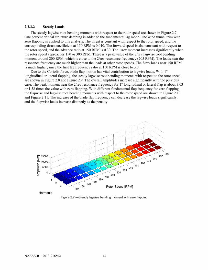
2.2.3.2 Steady Loads The steady lagwise root bending moments with respect to the rotor speed are shown in Figure 2.7.

One percent critical structure damping is added to the fundamental lag mode. The wind tunnel trim with zero flapping is applied to this analysis. The thrust is constant with respect to the rotor speed, and the corresponding thrust coefficient at 150 RPM is 0.010. The forward speed is also constant with respect to the rotor speed, and the advance ratio at 150 RPM is 0.30. The 1/rev moment increases significantly when the rotor speed approaches 150 or 300 RPM. There is a peak value of the 2/rev lagwise root bending moment around 200 RPM, which is close to the 2/rev resonance frequency (205 RPM). The loads near the resonance frequency are much higher than the loads at other rotor speeds. The 3/rev loads near 150 RPM is much higher, since the first lag frequency ratio at 150 RPM is close to 3.0.

Due to the Coriolis force, blade flap motion has vital contribution to lagwise loads. With 1° longitudinal or lateral flapping, the steady lagwise root bending moments with respect to the rotor speed are shown in Figure 2.8 and Figure 2.9. The overall amplitudes increase significantly with the previous case. The peak moment near the 2/rev resonance frequency for 1° longitudinal or lateral flap is about 3.03 or 1.38 times the value with zero flapping. With different fundamental flap frequency for zero flapping, the flapwise and lagwise root bending moments with respect to the rotor speed are shown in Figure 2.10 and Figure 2.11. The increase of the blade flap frequency can decrease the lagwise loads significantly, and the flapwise loads increase distinctly as the penalty.

Figure 2.7.—Steady lagwise bending moment with zero flapping

NASA/CR—2013-216502 14

Figure 2.8.—Steady lagwise root bending moment with 1° longitudinal flap.

Figure 2.9.—Steady lagwise root bending moment with 1° lateral flap.

NASA/CR—2013-216502 15

Figure 2.10.—Flapwise loads with different flap stiffness.

Figure 2.11.—Lagwise loads with different flap frequencies.

NASA/CR—2013-216502 16

For rigid blade modeling in hover, the relations between the flap motion and the cyclic pitch controls are (Ref. 49)

𝜃1𝑐 = 8𝛾𝜈𝛽2 − 1𝛽1𝑐 + 𝛽1𝑠 (23)

𝜃1𝑠 = 8𝛾𝜈𝛽2 − 1𝛽1𝑠 − 𝛽1𝑐 (24)

Usually, 𝜈𝛽 is very close to 1.0. For different flap frequency ratios, the cyclic pitch controls are shown in Figure 2.12. The Lock number 7.58 is adopted in the calculation. The increase of fundamental flap frequency ratio causes significant increase of pitch controls. The limitation of pitch controls causes trim problems. The insufficient flap motion from the pitch controls makes the helicopter alter its altitude to generate enough forces and moments to trim the helicopter.

From the above analysis, the blades undergo high lagwise loads when operating around the lagwise resonance area. For the consideration of blade strength and fatigue, it is of great importance to avoid long time working at these rotor speeds. In present research, the rotor speed will go through from 180 to 240 RPM, or inversely, to prevent rotor blades from high loads. With the consumption of fuel, the optimum rotor speed decreases slowly with the helicopter gross weight (Ref. 50). When the rotor speed reaches the boundary of the resonance area, it goes through the dangerous region very quickly to avoid high loads, as seen in Figure 2.13. The baseline crossing time is 10 sec.

Figure 2.12.—Relations between pitch controls and flap motion in hover.

NASA/CR—2013-216502 17

Figure 2.13.—The scheme of the rotor speed with time.

Figure 2.14.—The time history of the rotor speed and its variation.

2.2.3.3 Identical Rotor Crossing 2/rev Resonance Area Baseline results are obtained for a forward flight condition, 𝜇 = 0.30 at half full rotor speed, and the

corresponding thrust coefficient 0.010. When the rotor speed changes, the forward speed and rotor thrust are kept constant, but the advance ratio and thrust coefficient will alter. The longitudinal tilt of the rotor tip plane can be simply calculated by

𝛽1𝑐 =12𝜌𝑉∞

2 𝑓𝜋𝑅2

𝜋𝑅2

𝐶𝑇𝜌𝜋𝑅2(Ω𝑅)2=

𝑓𝜋𝑅2

𝜇2

2𝐶𝑇 (25)

f /πR2 typically falls between 0.004 (clean designs) and up to 0.025 (heavy-lift transport or first-generation helicopters) (Ref. 49). In present example, 0.004 is adopted, and the corresponding β1c is 1.03°. In the baseline example, 1° longitudinal flap is applied. The lateral tilt is set to zero. The time histories of the rotor speed and the variation of rotor speed (Ω) are shown in Figure 2.14. The variation of rotor speed increases firstly then decreases. Every 10 RPM, the pitch controls are provided by the steady trim. The pitch controls between the discrete values are calculated by the curve-fit method. The pitch controls accompanying the variation of rotor speed are shown in Figure 2.15.

NASA/CR—2013-216502 18

Figure 2.15.—The time history of the pitch controls.

The time histories of the lagwise root bending moment of blade-2 and the rotor torque are shown in Figure 2.16. The lagwise root bending moment is amplified significantly during 10 to 12 sec. The FFT (Fast Fourier Transform) analysis illustrates that the resonance frequency (6.84 Hz/410 RPM) is exactly twice the rotor speed at that instant, which means the resonance frequency is 2/rev. The corresponding time histories of the thrust and the flapwise displacement of the blade tip are shown in Figure 2.17. During the resonance crossing, the variation of the rotor thrust and the flapwise tip displacement are substantially small.

The variation of rotor torque is substantially small during the resonance crossing. The shape of the rotor torque is the same as the rotor speed. The transient 2/rev lagwise root bending moment has not been transferred to the hub. The static rotor torque at the low rotor speed (180 RPM) is much smaller than that at high rotor speed (240 RPM), which shows that reducing rotor speed in forward flight can reduce the required rotor power. It is economical to decrease rotor speed in forward flight.

NASA/CR—2013-216502 19

Figure 2.16.—The lagwise root moment and rotor torque with 1° longitudinal flap.

Figure 2.17.—The time histories of rotor thrust and flapwise tip displacement.

NASA/CR—2013-216502 20

Figure 2.18.—The time histories of the lagwise root bending moment

and the rotor torque without the variation of rotor speed. During the transient process, there is a sharp increase of the rotor torque. Figure 2.18 shows the time

history of the rotor torque without the variation of rotor speed (Ω). The sharp increase of the static rotor torque disappears. The inertia of the rotor is 2880 kg/m2. At the instant 10.62 sec, the angular acceleration is 0.968 rad/sec2. The extra torque introduced by the rotor inertia is 2788 Nm. This value is about the difference between the transient torque with the variation of rotor speed at that instant and the torque without the variation. To reduce the sharp increase of the rotor torque, it is necessary to limit the acceleration of rotor rotation (Ω).

2.2.3.3.1 Influence of Flap Motion Previous analysis has pointed out that flap motion has significantly influence on steady lagwise loads.

Figure 2.19 and Figure 2.20 show the time histories of the lagwise root bending moment and rotor torque for different longitudinal flapping. The flap motion has significant influence on the transient peak-peak moment. The peak-peak lagwise root bending moment with 1°, 2° and 3° longitudinal flapping is 3.13, 7.77 and 14.01 times that with zero flapping, respectively. With the increase of the flapping, the variation of the rotor torque during the resonance crossing also increases significantly. The FFT analysis of the rotor torque with 3° longitudinal flapping during the resonance crossing illustrates that the dominative frequency of the peak torque is 14.17 Hz. That is four times the frequency of the rotor speed at that instant. The 4/rev lagwise load is transferred to the rotor hub, since large flapping causes large higher harmonic loads. The level of rotor flapping during the resonance crossing is very important to the peak loading in the lead-lag direction. It is important to consider the dynamic trim or proper time histories of cyclic and collective pitch controls to control the resonance loads.

NASA/CR—2013-216502 21

Figure 2.19.—Lagwise root bending moment for different flapping.

Figure 2.20.—Rotor torque for different flapping.

2.2.3.3.2 Influence of the Duration During the Transient Process The acceleration of rotor rotation is determined by the duration from the initial instant of the rotor

speed to the terminal instant. Figure 2.21 shows the responses of the lagwise root bending moment for different durations. The lagwise root bending moment increases with the increase of the duration. The peak-peak moment increases by 37.2 percent, when the duration increases from 5 to 20 sec. Figure 2.22 shows the time histories of the rotor torque with different durations. The maximum rotor torque decreases significantly with the increase of the duration. The maximum value decreases by 46.3 percent, when the period varies from 5 to 20 sec. Long duration causes high lagwise loads, and short duration causes high rotor torque due to the large variation of rotor speed. It is necessary to balance the duration to cross the resonance area.

NASA/CR—2013-216502 22

Figure 2.21.—Lagwise root bending moment for different rotor

speed variation durations.

Figure 2.22.—Rotor torque for different rotor speed variation duration.

2.2.3.3.3 Influence of Forward Speed Helicopter forward speed is limited by the shock wave in advancing blades and stall in retreating

blades. The reduction of the rotor speed can help to alleviate the shock wave. But it aggravates the stall. In present example, the maximum advance ratio at half full rotor speed is 0.4 (136 km/h), and the corresponding advance ratio at the full rotor speed is 0.2. The peak-peak lagwise root bending during the resonance crossing for different forward speeds are shown in Figure 2.23. The moment increases significantly with the forward speed. The influence of the flapping is obvious. For the consideration of blade strength, varying the rotor speed at lower forward speed could help to reduce the loads during the resonance crossing.

NASA/CR—2013-216502 23

Figure 2.23.—The influence of forward speed on the

peak-peak lagwise root bending moment.

Figure 2.24.—The influence of rotor thrust on the lagwise

root bending moment.

2.2.3.3.4 Influence of Rotor Thrust The influence of the rotor thrust on the peak-peak lagwise root bending moment during the resonance

crossing is shown in Figure 2.24. The forward speed is 102 km/h with wind tunnel trim. The baseline thrust is corresponding to the thrust coefficient 0.010 at half rotor speed. Thirty percent increase of the rotor thrust causes 50.7 and 21.3 percent increase of the peak-peak moment for 0° and 1° longitudinal flapping respectively. Thirty percent decrease of the rotor thrust causes 40.6 and 21.1 percent reduction of the moment. It is better to change the rotor speed at low thrust to reduce transient loads during resonance crossing.

NASA/CR—2013-216502 24

Figure 2.25.—Dissimilarity at 0.6 to 0.7R.

2.2.3.4 Dissimilar Rotor Crossing 2/rev Resonance Area Usually, the manufacturing tolerance among all blades of a rotor is limited to some small value to

achieve static and dynamic balance. Not only manufacturing tolerance, but also some other factors introduce rotor dissimilarities—battle damage to military helicopter rotors, moisture absorption, loss of trim mass, a nonoperational lag damper and so on (Refs. 51 to 53). These blade faults usually result in a change of mass distribution, bending stiffness, torsional stiffness, lag damping, and so on. In this work, the practice in (Ref. 53) is followed to deal with the rotor dissimilarities. The baseline dissimilarity is simulated by the modification of blade material property at 0.6 to 0.7R, as seen in Figure 2.25.

2.2.3.4.1 Unbalanced Mass The time history of the lagwise root bending moment and the rotor torque are shown in Figure 2.26,

when the blade-2 mass distribution is reduced by 5 percent at 0.6 to 0.7R. The wind tunnel trim with 1° longitudinal flapping is applied. In the following analysis, this trim is adopted. The variation of the lagwise root bending moment is substantially small compared with Figure 2.16. The rotor torque increases significantly during the resonance crossing. The difference of mass distribution among different blades introduces unbalanced lagwise root bending moments, and the unbalanced moments are transferred to the rotor hub, then generate sharp rise in the torque response. The frequency of the major component of the transient response is 6.84 Hz. Obviously, this frequency is the 2/rev component at that instant.

2.2.3.4.2 Influence of Blade Stiffness The influence of the flap, lag and torsional stiffness on the transient rotor torque is substantially small,

when the stiffness is reduced by 5 percent at 0.6 to 0.7R.

2.2.3.4.3 Influence of Blade Lag Damping To investigate the influence of the blade damping on the transient loads, the critical damping of every

blade is increased from 1 to 5 percent. The time responses of the lagwise root bending moment and the rotor torque are shown in Figure 2.27, when the blade-2 mass distribution is reduced by 5 percent at 0.6 to 0.7R. The increase of the blade lag damping can significantly reduce the transient loads during the resonance crossing. The peak-peak lagwise root bending moment is reduced by 64.9 percent. The rotor torque is reduced to the level without the dissimilarity. The increase of the blade lag damping is an effective means to control the transient loads during the lagwise resonance crossing. However, introducing 5 percent critical lag damping into stiff in-plane blades is a difficult task due to the small rotation of blade root and the high blade stiffness.

NASA/CR—2013-216502 25

Figure 2.26.—Lagwise root bending moment and rotor toque with

5 percent mass dissimilarity.

Figure 2.27.—Lagwise root bending moment and rotor torque with

5 percent critical damping.

NASA/CR—2013-216502 26

2.2.3.4.4 Dissimilarity in Two Blades In the previous analysis, one blade property is modified. When the mass distribution of blade-2 and

blade-3 is reduced by 5 percent simultaneously at 0.6 to 0.7R, the time history of the rotor torque is shown in Figure 2.28. The rotor torque is almost the same as the baseline rotor torque shown in Figure 2.16 during the 2/rev resonance crossing. When the mass distribution of blade-2 and blade-4 is reduced by 5 percent at 0.6 to 0.7R, the time history of the rotor torque is also shown in Figure 2.28. It is amplified significantly. From the above analysis, it can be concluded that the modifications of two blade mass distributions can cause the lagwise root bending moments to cancel each other, or inversely to superimpose together depending on their phase relation.

The principles determining the phenomenon during steady states are applied to explain why the lagwise root bending moments superimpose together when the mass distribution of blade-2 and blade-4 is modified; on the contrary, they seem to cancel each other when the mass distribution of blade-2 and blade-3 is altered. The lagwise root bending moment with baseline blade property can be expressed as

𝑀 = 𝑀0 + ∑ [𝑀𝑛𝑐 cos(𝑛𝜓𝑚) +𝑀𝑛𝑠sin (𝑛𝜓𝑚)]𝑛𝑛=1 (26)

the lagwise root bending moment with modified blade property can be expressed as

𝑀′ = 𝑀0′ +∑ [𝑀𝑛𝑐

′ cos(𝑛𝜓𝑚) + 𝑀𝑛𝑠′ sin (𝑛𝜓𝑚)]𝑛

𝑛=1 (27)

since the maximum harmonic component of the lagwise root bending moment is 2/rev during the 2/rev resonance crossing, the analysis of 2/rev load is specified. When the mass distribution of blade-2 and blade-3 is reduced, the 2/rev rotor torque is

𝑄2 = 𝑀2𝑐 cos(2𝜓𝑚) + 𝑀2𝑠 sin(2𝜓𝑚) + 𝑀2𝑐′ cos 2 𝜓𝑚 + 𝜋

2 + 𝑀2𝑠

′ sin 2 𝜓𝑚 + 𝜋2

+𝑀2𝑐′ cos 2(𝜓𝑚 + 𝜋) + 𝑀2𝑠

′ sin 2(𝜓𝑚 + 𝜋) +𝑀2𝑐 cos 2𝜓𝑚 + 3𝜋2 + 𝑀2𝑠 sin 2𝜓𝑚 + 3𝜋

2 = 0 (28)

if the mass distribution of blade-2 and blade-4 is reduced, the 2/rev rotor torque is

𝑄2′ = 2(𝑀2𝑐 −𝑀2𝑐′ ) cos(2𝜓𝑚) + 2(𝑀2𝑠 −𝑀2𝑠

′ ) sin(2𝜓𝑚) (29)

Equation (28) illustrates that the lagwise root bending moments of blade-2 and blade-3 cancel each other due to the phase difference 𝜋 2⁄ . The phenomenon illustrated in Equation (29) is on the contrary.

Figure 2.28.—Rotor torque with two blade dissimilarity.

NASA/CR—2013-216502 27

2.2.3.5 Higher Stiffness Rotor During 4/rev Resonance Crossing To investigate the dynamics of variable speed rotor during 4/rev resonance crossing, the lag stiffness

of the blade shown in Table 2.1 is increased to four times its original value. Other parameters of the rotor are kept at the same values. The variation of the fundamental lag frequency with respect to the rotor speed is shown in Figure 2.29, which illustrates that the rotor goes through the 3/rev (270 RPM) resonance area and the 4/rev (202 RPM) resonance area.

The time histories of the lagwise root bending moment of blade-2 and the rotor torque are shown in Figure 2.30. The variation of the lagwise root bending moment is substantially small. There is a sharp rise of rotor torque during 8 to 10 sec. The FFT analysis shows that the resonance frequency is 13.19 Hz, which is about four times 3.36 Hz. The 4/rev lagwise root bending moment is transferred to the rotor hub. The steady response of the rotor torque during the first 5 sec is much larger than that shown in Figure 2.14. It is obvious that stiffer blades introduce larger variation of rotor torque.

The time histories of the blade-2 lagwise root bending moment and rotor torque are shown in Figure 2.31, when the mass distribution of blade-2 is reduced by 5 percent at 0.6 to 0.7R using the higher lag stiffness. The variation of the lagwise root bending moment is substantially small compared with the above response. The rotor torque is similar to that of the identical rotor.

The critical damping of every blade is increased to 5 times the original value of the identical rotor. The time responses of the lagwise root bending moment and the rotor torque are shown in Figure 2.32. The increase of blade lag critical damping can significantly reduce the transient loads during the resonance crossing. The maximum rotor torque is decreased by 24.6 percent.

Figure 2.29.—Frequency versus rotor speed for the higher lag stiffness blade.

NASA/CR—2013-216502 28

Figure 2.30.—Baseline lagwise root bending moment when crossing 4/rev

resonance area.

Figure 2.31.—Response with higher lag stiffness and 5 percent mass

dissimilarity.

NASA/CR—2013-216502 29

Figure 2.32.—Reponses with five times the original damping.

2.2.4 Summary and Conclusions In this research, an aeroelastic simulation is employed to analyze the dynamic characteristics of a

four-blade stiff in-plane rotor during resonance crossing. Based on the 2/rev resonance crossing analysis, the following can be concluded:

• For identical rotors, 2/rev lagwise root bending moment of single rotor blade is amplified

significantly during the resonance crossing, and the variation of rotor torque is substantially small. • The flap motion contributes significantly to the lagwise loads, whether in steady state or in

transient process. One degree longitudinal flap causes 213 percent increase of the peak-peak lagwise root bending moment compared with the zero flapping case. It is important to reduce the flapping during the resonance crossing to control the transient loads.

• Increasing the duration during the resonance crossing amplifies the peak-peak lagwise root bending moment, and decreases the maximum rotor torque.

• Varying the rotor speed at lower forward speed or lower thrust could help to reduce the transient loads.

• Five percent reduction of blade mass at 0.6 to 0.7R has significant influence on the transient rotor torque. Five percent blade critical damping significantly reduces the rotor torque to the level without dissimilarity. The peak-peak lagwise root bending moment is reduced by 64.9 percent.

• The 5 percent reduction of flap lag, or torsional stiffness at 0.6 to 0.7R has substantially small influence on the transient lagwise root bending moment and rotor torque.

• The dissimilarity in two blades can cancel each other, or inversely superimpose together depending on their phase relation.

• Based on the 4/rev resonance crossing analysis, the following can be concluded: • For identical rotor, 4/rev lagwise root bending moment is transferred to the rotor shaft, and a

sharp rise of 4/rev rotor torque occurs. • For dissimilar rotor with 5 percent reduction of one blade mass distribution at 0.6 to 0.7R, 4/rev

lagwise root bending moment is also transferred to the rotor shaft. • Increasing blade lag damping significantly reduces the maximum transient rotor torque.

NASA/CR—2013-216502 30

From the summary of present study, it can be concluded that attention should be paid to blade strength during resonance crossings. It is seriously dangerous for dissimilar rotors to go through resonance crossing, which perhaps will cause some damages to transmission shafts, gears and engines.

2.3 Transient Loads Control of a Variable Speed Rotor during Lagwise Resonance Crossing

2.3.1 Introduction For some variable speed rotors, lagwise loads can increase sharply during the lagwise resonance

crossing (Ref. 54). For example, the fundamental natural frequency of the lag motion for uniform rotor blade with lag hinge offset and hinge spring is

𝜈𝜁2＝32

𝑒1−𝑒

+ 𝑘𝜁𝐼𝑏𝛺2(1−𝑒)

(30)

Typical values of 𝑒 in normal conditions are small. If rotor speed decreases by 50 percent, the fundamental lag frequency will increase by about 100 percent. For typical stiff in-plane rotors (𝜈𝜁= 1.4-1.6/rev in full rotor speed), they go through the 2/rev resonance area. Rotor blades have to undergo these high transient loads. The transfer of these severe loads to transmission systems affects the working condition of the transmission systems, which might damage the transmission shafts, gears or engines. It is highly necessary to control these high transient resonance loads to protect rotor blades and transmission systems.

For articulated or soft in-plane rotors, large lag dampers are attached to blade root. These lag dampers can enhance the stability of the rotor-fuselage system and can also suppress the sudden rise of lagwise transient loads. For stiff in-plane rotors, the ground or air resonance problems disappear. Lag dampers are not typically required from these rotor systems. For stiff in-plane variable speed rotors during large variation of rotor speed, how to manage the high transient loads during resonance crossing can be an important and challenging problem to solve. Usually, structural damping is very low, and the lag damping introduced by aerodynamics is weak. For stiff in-plane rotors, it is difficult to provide enough lag damping through traditional root dampers due to the small deformations at blade root, and large blade lag stiffness.

Zapfe and Lesieutre put forward the concept of distributed inertial dampers using chordwise absorbers to provide damping to the beam structure (Ref. 55). Results demonstrated the effectiveness using a simply supported beam under tensile load. Hébert and Lesieutre utilized highly distributed tuned vibration absorbers to provide lag damping to helicopter blades (Ref. 56). Their studies illustrated that method could provide enough damping with a weight penalty equal to only 3 percent blade mass. Kang, Smith and Lesieutre carried out a comprehensive analysis of the damping characteristics of a rotor blade with an embedded chordwise absorber (Refs. 57 to 59). The potential large stroke of elastomeric dampers was a major obstacle for the application of the elastomeric dampers due to the limited space in the blade cavity. The concept of fluidlastic dampers was introduced to reduce the stroke. Petrie, Lesieutre and Smith utilized embedded fluid elastomer absorber to enhance blade lag damping, and conducted the fluid-elastomer design and the lag damping test of a blade with a fluid-elastomer absorber (Ref. 60 and 61). Han and Smith introduced embedded chordwise absorbers to reduce blade lagwise loads, and their investigations indicated that placing an embedded chordwise absorber at blade tip could significantly reduce the 1/rev or 2/rev lagwise load (Ref. 57). The embedded chordwise fluidlastic damper shown in Figure 2.33 presents a feasible means to provide enough lag damping to stiff in-plane rotors.

NASA/CR—2013-216502 31

Figure 2.33.—Configuration of embedded chordwise damper

2.3.2 Research Objectives This research focuses on the simulation and control of the transient loads of a variable speed rotor

during resonance crossing. The feasibility of embedded chordwise fluidlastic dampers is explored. A device design procedure to select parameters such as mass, loss factor, tuning frequency, and tuning port area ratio is developed. The system modeling of helicopter rotor with embedded chordwise dampers is presented. A hypothetical stiff in-plane rotor is analyzed during resonance crossing. Transient aeroelastic responses are calculated to evaluate the performance of the fluidlastic dampers to reduce the transient blade lagwise loads. Comprehensive parametric study including tuning frequency, loss factor, tuning port ratio, tuning mass, blade flapping motion, duration during resonance and flight states on the performance of embedded fluidlastic dampers are investigated.

2.3.3 Analytical Model

2.3.3.1 Modeling of a Rigid Blade With a Fluidlastic Damper The viscoelastic behavior of the elastomeric spring of the fluidlastic damper in frequency domain is

simulated by

𝒌𝒂∗ = 𝒌𝒑(𝟏+ 𝒊𝜼) (31)

The configuration of the mathematical modeling of a fluidlastic damper is shown in Figure 2.34. The inertia of the fluidlastic damper can be amplified by the tuning mass through the leverage effect. Larger G can be utilized to reduce the weight and stroke. That is the vital benefit of fluidlastic dampers different from elastomeric dampers (Ref. 57). The natural frequency of the fluidlastic damper is

𝝎𝒏 = 𝒌𝒑

𝒎𝒑+(𝑮−𝟏)𝟐𝒎𝒕 (32)

To evaluate how much damping is provided to the rotor blade, a two degree-of-freedom model of a rigid blade with a fluidlastic damper is employed from Petrie’s work (Ref. 62). The equations of motion for the system are

𝐌 𝒑+ 𝐊

𝝃𝒂𝒑

= 𝐅 (33)

NASA/CR—2013-216502 32

Figure 2.34.—Mathematical modeling of fluidlastic damper.

Where

𝐌 = ∫ 𝒎(𝒓 − 𝒆)𝟐𝒅𝒓𝑹𝒆 + 𝒎𝒑 + 𝒎𝒕(𝒓 − 𝒆)𝟐 −𝒎𝒑 −𝒎𝒕(𝑮− 𝟏)(𝒓𝒂 − 𝒆)

−𝒎𝒑 −𝒎𝒕(𝑮 − 𝟏)(𝒓𝒂 − 𝒆) 𝒎𝒑 +𝒎𝒕(𝑮 − 𝟏)𝟐 (34)

𝐊 = ∫ 𝒎(𝒓 − 𝒆)𝒆𝛀𝟐𝒅𝒓𝑹𝒆 + 𝒌𝝃 + 𝒎𝒑 + 𝒎𝒕(𝒓 − 𝒆)𝒆𝛀𝟐 −𝒎𝒑 −𝒎𝒕(𝑮 − 𝟏)𝒆𝛀𝟐

−𝒎𝒑 −𝒎𝒕(𝑮 − 𝟏)𝒆𝛀𝟐 𝒌𝒂∗ − 𝒎𝒑 + 𝒎𝒕(𝑮− 𝟏)𝟐𝛀𝟐 (35)

𝐅 = ∫ 𝑭𝝃(𝒓 − 𝒆)𝒅𝒓𝑹𝒆 + 𝒎𝒑𝒆𝛀𝟐𝒂𝒑𝟎 + 𝒎𝒕𝒆𝛀𝟐𝒂𝒕𝟎

𝒎𝒑𝛀𝟐𝒂𝒑𝟎 −𝒎𝒕(𝑮 − 𝟏)𝛀𝟐𝒂𝒕𝟎 (36)

The eigenvalues and eigenvectors of the coupled system are analyzed to calculate the blade damping. To evaluate the stroke of the fluidlastic damper, 1° blade tip motion is given to calculate the stroke of the damper.

Under static state, the spring acts on the prime mass and the fluid has no effect on the static displacement of the damper. In this way, the static displacement of the prime mass can be reduced significantly due to the large spring. Under rotation, the embedded damper must undergo large centrifugal force. The fluid is encapsulated in the damper with physical restriction, which can limit the variation of the mass center of the damper.

To estimate how much the in-plane loads can be reduced during the resonance crossing, the rotor response is calculated in the time domain using a comprehensive rotor code. The harmonic excitations in the lagwise direction are integral times the rotor speed. During the resonance crossing, the major excitation is the resonance frequency. In this report, the baseline variable speed rotor goes through the 2/rev resonance area, and the 2/rev rotor speed (2Ω) is utilized as the excitation frequency (ω) to the damper. The corresponding steady solution for the single excitation can be expressed by Aeiωt. A is the amplitude of the response. For the single degree-of-freedom modeling of the fluidlastic damper, the relation for the equivalent of the imaginary part is

𝒄𝒑𝝎 = 𝜼𝒌𝒑 (37)

From the definition of the critical damping 𝜻 = 𝒄𝒑/[𝟐𝝎𝒏(𝒎𝒑 + (𝑮 − 𝟏)𝟐𝒎𝒕)], the relation between the critical damping and the excitation frequency is

𝜻(𝝎) = 𝜼𝝎𝒏𝟐𝝎

(38)

The above equation illustrates that the critical damping decreases with the rotor speed.

NASA/CR—2013-216502 33

2.3.3.2 Comprehensive Rotor Modeling With Fluidlastic Dampers The comprehensive rotor modeling follows References 54 and 42. A moderate deflection beam model

is employed to describe the elastic deformations of rotor blades. Rigid rotations including blade hinges and rotor rotation degree are introduced based on the generalized force formulation (Ref. 45). Quasi-steady aerodynamics with table look-up aerofoil aerodynamics is utilized to describe the blade aerodynamics. The rotor induced velocity in the steady and transient states is captured by the Pitt-Peters dynamic inflow model.

For trusted analysis, a time domain model of fluidlastic damper device is required. One degree-of-freedom model of the fluidlastic damper is coupled with the rotor modeling. The device is mechanically constrained to move only in the blade chordwise direction. The relative displacements of the prime mass and the tuning mass of the absorber to the blade are denoted as ap+ap0 and at+at0. The position vector of the prime mass can be expressed as

𝑹𝒑𝒙𝑹𝒑𝒚𝑹𝒑𝒛

𝑻

=

𝒅𝒐𝒇𝟎𝟎

𝑻

[𝑻𝒓𝒔] + 𝒅𝒇𝒍𝟎𝟎

𝑻

𝑻𝒇𝒓[𝑻𝒓𝒔] + 𝒅𝒍𝒑𝟎𝟎

𝑻

𝑻𝒍𝒇𝑻𝒇𝒓[𝑻𝒓𝒔] + 𝒙 + 𝒖𝒗𝒘

𝑻

𝑻𝒑𝒍𝑻𝒍𝒇𝑻𝒇𝒓[𝑻𝒓𝒔] +

𝟎

𝒂𝒑 + 𝒂𝒑𝟎𝟎

𝑻

[𝑻]𝑻𝒑𝒍𝑻𝒍𝒇𝑻𝒇𝒓[𝑻𝒓𝒔] (49)

The relation of the prime mass with the tuning mass is

𝒂𝒕 = −(𝑮 − 𝟏)𝒂𝒑 (50)

Then the relative displacement of the tuning mass to the blade can be expressed as

𝑹𝒕𝒙𝑹𝒕𝒚𝑹𝒕𝒛

𝑻

=

𝒅𝒐𝒇𝟎𝟎

𝑻

[𝑻𝒓𝒔] + 𝒅𝒇𝒍𝟎𝟎

𝑻

𝑻𝒇𝒓[𝑻𝒓𝒔] + 𝒅𝒍𝒑𝟎𝟎

𝑻

𝑻𝒍𝒇𝑻𝒇𝒓[𝑻𝒓𝒔] + 𝒙 + 𝒖𝒗𝒘

𝑻

𝑻𝒑𝒍𝑻𝒍𝒇𝑻𝒇𝒓[𝑻𝒓𝒔] +

𝟎

−(𝑮 − 𝟏)𝒂𝒑 + 𝒂𝒕𝟎𝟎

𝑻

[𝑻]𝑻𝒑𝒍𝑻𝒍𝒇𝑻𝒇𝒓[𝑻𝒓𝒔] (51)

The tangent mass, stiffness, damping matrices and generalized force vector introduced by the kinetic energy can be calculated according to the definition in References 42 and 45 using the above position vectors. The elastic potential energy is 𝟏𝟐𝒌𝒑𝒂𝒑𝟐, and the work done by the viscous force is 𝟏𝟐𝒄𝒑𝒑𝟐. The fluidlastic damper thus contributes to the generalized force, tangent stiffness and damping matrices.

Assembling the three components including structure, kinetics and aerodynamics, the equations of motion based on the generalized force formulation are achieved. The implicit Newmark integration method is utilized to calculate the steady and transient responses in time domain. Every rotor blade is discretized by the 15 degree-of-freedom beam elements, as seen in Figure 2.35.

NASA/CR—2013-216502 34

Figure 2.35.—Rotor-damper system.

The variation of the rotor speed is prescribed during the resonance crossing in forward flight. To

maintain the rotor thrust and forward speed, pitch controls need to be provided to the rotor. A dynamic wind-tunnel trim is utilized to provide the time histories of the pitch controls. The pitch controls in steady state for several discrete rotor speeds are trimmed for the same thrust and forward speed. During the variation of the rotor speed, the pitch controls between two rotor speeds are calculated using the curve-fit method.

2.3.4 Embedded Chordwise Damper Design The design of embedded chordwise fluidlastic dampers follows Reference 61. The objective in this

section is to decrease the transient lagwise loads during the resonance crossing to the level in steady state. The weight of the damper is limited to 5 percent blade gross weight, and the stroke is restricted to 5 percent blade chord length due to the limited space in blade airfoil cavity. For the design of fluidlastic dampers, the tuning port area ratio (G) is one of the key parameters. From the view of practical application, a suitable G=40 is adopted in the baseline design. The parameters of the fluidlastic damper could be optimized and determined to satisfy the design objectives, which include tuning frequency, loss factor, prime mass, tuning mass and tuning port area ratio. The design flowchart is shown in Figure 2.36. From the general considerations, smaller damper mass, large G and the setup location of the damper at the blade tip are preferred. Some parameters of the damper are shown in Table 2.2.

TABLE 2.2.—EMBEDDED CHORDWISE DAMPER PARAMETERS

Prime mass, kg ........................................................ 1.0 Tuning mass, kg ...................................................... 1.0 Tuning port area ratio ............................................... 40 Damper radial position ................................... Blade tip

NASA/CR—2013-216502 35

Figure 2.36.—Design flowchart.

Figure 2.37 shows the rotating frequencies of the blade and damper, and the blade lag damping with respect to the rotor speed. The loss factor is 0.4. The blade lag damping increases initially then decreases with the rotor speed. The tuning frequency of the damper has significant influence on the blade damping. The peak blade damping decreases with the increase of the tuning frequency. Since the resonance occurs at the rotor speed 205 RPM, the damper is tuned to 7.2 Hz. When the damper is tuned to 7.2 Hz, the blade lag damping and dynamic stroke with respect to the rotor speed for different loss factors are shown in Figure 2.38. When loss factor is 0.3, the peak damping of the blade is more than 8 percent. The bandwidth performance is much better than other cases around the resonance rotor speed. Within 180~230 RPM, the blade critical damping is above 6 percent. The stroke of the damper decreases significantly with the increase of the loss factor. From the above analysis, the damper needs to be tuned to 7.2 Hz with loss factor 0.3.

NASA/CR—2013-216502 36

Figure 2.37.—Blade damping and rotating frequencies versus rotor speed

for different tuning frequencies (η=0.4).

Figure 2.38.—Blade damping and the stroke versus rotor speed for

different loss factors (ωn=7.2 Hz).

NASA/CR—2013-216502 37

2.3.5 Transient Loads Control Via Embedded Damper With the design parameters of the damper, the responses of the blade and damper can be calculated.

The comparison between the transient response with the damper and the response without the damper can be utilized to evaluate the performance of the damper. It is necessary to check whether the displacement response of the damper is within the design limit or not. Due to the difference between the two models, the analysis of the influence of the tuning frequency and loss factor on the performance of the damper using the comprehensive code is needed to verify the design modeling.

The prime mass, tuning mass and tuning port area ratio of the fluidlastic damper are as specified in Table 2.2. Since the blades go through the 2/rev resonance area, the primary excitation frequency in the damper modeling is 2.0 times the rotor speed. The moment ratio is defined as the ratio of the peak-peak lagwise root bending moment with the fluidlastic damper during 5 to 15 sec to the peak-peak moment without the fluidlastic damper. The stroke ratio is defined as the stroke of the damper divided by the blade chord length.

For traditional absorbers, isolators or dampers, tuning frequency is one of the key design parameters. For different natural frequencies and loss factors, the moment ratios and stroke ratios are shown in Figure 2.39 and Figure 2.40, respectively. With the increase of the loss factor, the moment ratio decreases firstly, then increases. In the range of the frequency from 5.6 to 8.0 Hz, the moment ratio also decreases firstly then increases. The stroke decreases significantly with the increase of loss factor. When the damper is tuned to 7.0 Hz with loss factor 0.2, the damper can reduce the peak-peak moment by 65.0 percent. The corresponding stroke is 0.72 percent blade chord length. When the damper is tuned to 6.9 Hz with loss factor 0.3, the peak-peak moment is reduced by 64.7 percent. The stroke decreases to 0.58 percent chord length. From the view of bandwidth, the damper with larger loss factor is obviously better than the one with smaller loss factor. With the variation of ±0.5 Hz tuning frequency or ±0.1 loss factor, about 50 percent peak-peak moment can be reduced. In the following analysis, the damper is tuned to 6.9 Hz with loss factor 0.3. These design parameters are very close to the parameters calculated by the two degree-of-freedom model, which illustrates the design using the simple modeling is an accurate and effective method.

The comparison of the time histories of the lagwise root bending moment and the stroke of the damper are shown in Figure 2.41. The steady loads in the first or last 5 sec increases compared with the case without the damper. The peak-peak moment with the damper during the resonance crossing increases by 7.61 percent the peak-peak moment at the first 5 sec. The stroke during the transient process is smaller than that in steady state. Figure 2.42 shows the comparison and the stroke, when the damper is tuned to 6.5 Hz with loss factor 0.05. The steady response in the first 5 sec decreases significantly. The damper also attenuates the transient loads during the resonance crossing, and the peak-peak moment is reduced by 27.0 percent. Obviously, the performance of the fluidlastic damper decreases significantly compared with the case with the tuning frequency 6.9 Hz and loss factor 0.3. The steady response in the last 5 sec has substantially small variation. From the above analysis, the side effect of the fluidlastic damper on the steady loads should be paid attention to. It can increase the steady loads, when it is tuned to its optimum value. The high transient loads usually exist for tens of seconds, but the blades have to undergo the steady loads for tens of hours for long endurance variable speed rotor helicopters. It is necessary to balance the benefits and side effects of fluidlastic dampers on transient and steady loads.

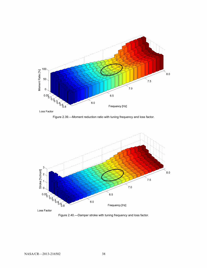
NASA/CR—2013-216502 38

Figure 2.39.—Moment reduction ratio with tuning frequency and loss factor.

Figure 2.40.—Damper stroke with tuning frequency and loss factor.

NASA/CR—2013-216502 39

Figure 2.41.—The comparison of moment response and the stroke of the

damper (6.9 Hz, 0.3 loss factor).

Figure 2.42.—The comparison of moment response and the stroke of the

damper (6.5 Hz, 0.05 loss factor).

2.3.6 Parametric Study For the optimization of the parameters of fluidlastic dampers, parametric studies are conducted in this

section to enhance the performance. The parameters includes tuning port area ratios, loss factors, device mass, blade flapping, the duration during resonance crossing, rotor thrust level, and forward speed.

Figure 2.43 shows the moment ratio, stroke and elastomeric stiffness versus tuning port area ratio. The damper is tuned to 6.9 Hz with loss factor 0.3 for all the cases. With the increase of the tuning port

NASA/CR—2013-216502 40

area ratio, the variation of the moment ratio is substantially small. The stroke decreases by 90.8 percent, when tuning port area ratio changes from 10 to 100. The elastomeric stiffness increases significantly with tuning port area ratio. Large tuning port area ratio is preferred in the design of fluidlastic dampers. Figure 2.44 shows the moment ratio, stroke and elastomeric stiffness versus prime mass. The gross weight of the prime mass and tuning mass is kept a constant value 2.0 kg. With the increase of the prime mass, the moment ratio and the stroke increase, and the elastomeric stiffness decreases. This means the reduction of the performance of the damper. When 0.5 kg prime mass is shifted as tuning mass, additional 23.8 percent peak-peak moment can be reduced. For the consideration of the gross weight of the damper, larger tuning mass and smaller prime mass are preferred.

Blade flap motion has vital contribution to blade lagwise loads. For different longitudinal flapping, the time histories of the root bending moment with and without the fluidlastic damper are shown in Figure 2.45. It is obvious that the transient loads increase significantly with the increase of blade flapping. The embedded chordwise damper can control the transient lagwise loads excellently during the resonance crossing. With 3.0° longitudinal flapping, the damper can reduce 65.7 percent peak-peak lagwise root bending moment. The corresponding time histories of the damper displacement are shown in Figure 2.46. The stroke of the damper increases significantly with the increase of the flapping. With 3.0° flapping, the stroke reaches 2.22 percent blade chord length.

Figure 2.43.—Moment ratio, stroke and elastomeric stiffness versus G

(ωn=6.9 Hz, η=0.3).

NASA/CR—2013-216502 41

Figure 2.44.—Moment ratio, stroke and elastomeric stiffness versus

prime mass (mp+mt=2.0 kg).

NASA/CR—2013-216502 42

Figure 2.45.—Time responses of lagwise root bending moment for

different flapping.

Figure 2.46.—Time responses of the displacement of the damper for

different flapping.

NASA/CR—2013-216502 43

Figure 2.47 shows the time histories of the lagwise root bending moment for different duration during the resonance crossing. With the increase of the duration, the damper can excellently control the loads. When the duration is 20 sec, the damper can reduce the peak-peak root bending moment by 66.3 percent. The corresponding time histories of the damper are shown in Figure 2.48. The stroke in transient is smaller than that in the first 5 sec. The maximum stroke is less than 1 percent blade chord length.

Figure 2.47.—Time responses of lagwise root bending moment for

different duration.

Figure 2.48.—Time responses of the displacement of the damper for

different duration.

NASA/CR—2013-216502 44

Figure 2.49 shows the moment ratio and stroke versus forward speed. With the increase of the forward speed during the resonance crossing, the variation of the moment ratio reduction is less than 5 percent. The stroke increases by 31.3 percent, when the forward speed increases from 34 to 136 km/h. Figure 2.50 shows the moment ratio and stroke versus rotor thrust. Within 60 percent variation of the rotor thrust, the variation of the moment ratio is less than 5 percent. The stroke increases significantly. With 30 percent increase of the rotor thrust, the stroke is less than 1 percent blade chord length. For different flight states, the variation of the performance of the damper is substantially small, and the stroke of the damper is limited to a low value (1 percent chord length).

Figure 2.49.—Moment ratio and stroke versus forward speed.

Figure 2.50.—Moment ratio and stroke versus thrust.

NASA/CR—2013-216502 45

2.3.7 Summary Embedded chordwise fluidlastic dampers are introduced to control rotor blade lagwise loads during

resonance crossing for variable speed stiff in-plane rotors. The design of the fluidlastic dampers based on the two degree-of-freedom blade-damper system model illustrates that more than 6 percent critical damping around the resonance rotor speed can be provided to the blade with less than 5 percent blade mass penalty. The analysis based on the elastic blade model illustrates:

• With the optimum combination of the tuning frequency and loss factor, the transient peak-peak

lagwise root bending moment can be reduced by 64.7 percent, and the corresponding stroke is less than 0.6 percent blade chord length. Within the variation of ±0.5 Hz tuning frequency or ±0.1 loss factor, about 50 percent peak-peak moment can be reduced.

• Larger tuning port area ratio and tuning mass need to be utilized to enhance the performance of the damper, and control the stroke of the fluidlastic damper. When tuning port area ratio changes from 10 to 100, the stroke can be reduced by 90.8 percent. When 0.5 kg prime mass is shifted as tuning mass, additional 23.8 percent peak-peak moment can be reduced.

• For different blade flapping, the damper can excellently control the transient lagwise loads. With 3.0° longitudinal flapping, the damper can reduce 65.7 percent peak-peak lagwise root bending moment, and the stroke is less than 2.5 percent blade chord length.

• For different period during the resonance crossing, the peak-peak transient loads can be reduced to the level in steady states.

• At different forward speed or thrust, the variation of the performance of the damper is substantially small, and the stroke is limited to a low value.

In a summary, the simple modeling is an accurate and effective method for the design of the

fluidlastic dampers. The embedded chordwise fluidlastic damper can excellently control the lagwise transient loads during the lagwise resonance crossing for the variable speed stiff in-plane rotors.

2.4 Rotor Modeling for System Integration

Variable speed rotors change rotor speeds according to flight states to optimize power consumption (Ref. 50). For the integration of the rotor modeling with the transmission and engine system modeling, blade lag motion is necessarily to be taken into account to capture the transfer of lag dynamics to rotor shaft dynamics. Blade flap motion has vital contribution to the lag motion due to the centrifugal force, and needs to be included in the comprehensive model. Different from typical helicopter rotors, variable speed rotors can vary their rotor speed degree to reduce rotor torque, the terms introduced by the variation of rotor speed should be taken into account in the modeling to explore the dynamics associated with the variation of rotor speed.

The modeling method derived by Jaw is utilized in the research (Ref. 63). The modeling can describe rigid blade dynamics with coupled flap and lag motions with the variation of rotor speed. The equations of motion for the coupled flap and lag motions are

−𝑀𝑒𝑥𝑡𝑖 = 𝐼𝑥𝑄𝑖 + 𝐼𝑥𝑄𝑖 + 𝑖2𝑐𝛽𝑖𝑠𝛽𝑖 +𝑚𝑖𝑒𝑦𝑔𝑅22𝑠𝛽𝑖𝑐𝜉𝑖 − 𝑚𝑖𝑒𝑦𝑔𝑅2𝑖𝑠𝛽𝑖𝑠𝜉𝑖 + 𝑚𝑖𝑔𝑦𝑔𝑅𝑐𝛽𝑖 (52)

𝐼𝑧𝑄𝑖 + 𝑖𝑐𝛽𝑖2 − 2𝐼𝑥𝑄𝑖𝑖 + 𝑖𝑐𝛽𝑖𝑠𝛽𝑖 + 𝐼𝑦𝑖 + 𝑖𝑠𝛽𝑖

2 +𝑏𝑙ℎ𝑖 + 𝑘𝜉𝜉 + 𝑚𝑖𝑒𝑦𝑔𝑅2𝑖𝑐𝛽𝑖𝑐𝜉𝑖 + 𝑚𝑖𝑒𝑦𝑔𝑅2𝑖2𝑐𝛽𝑖𝑠𝜉𝑖 = −𝑁𝑒𝑥𝑡𝑖 (53)

The expressions for the externally applied aerodynamics on the blade are

−𝑀𝑒𝑥𝑡𝑖 = ∫ (𝑟 − 𝑒)𝐹𝑧𝑑𝑟𝑅𝑟𝑅

(54)

NASA/CR—2013-216502 46

−𝑁𝑒𝑥𝑡𝑖 = ∫ (𝑟 − 𝑒)𝐹𝑥𝑑𝑟𝑅𝑟𝑅

(55)

For the general description of variable speed rotors, the term associated with the lag spring is added to the equation for the lag motion.

A nonlinear quasi-steady aerodynamic model is utilized, and the lift, drag, and moment coefficients of the aerofoil are calculated by a two-dimensional table-look-up method according to the angle of attack and the oncoming air flow (Mach number). The expressions for the lift and drag of the aerofoil are

𝐹𝑧 = 12𝜌𝑉

2𝑐𝐶𝑙 + 𝜌𝜋𝑏2ℎ − 𝑎ℎ𝑏 + 𝜌𝜋𝑏𝑉 (56)

𝐹𝑥 = 12𝜌𝑉

2𝑐𝐶𝑑 (57)

where

𝑉 = 𝑈𝑇2 + 𝑈𝑃2 (58)

𝛼 = 𝜃 − 𝑎𝑟𝑐𝑡𝑎𝑛𝑈𝑃𝑈𝑇 (59)

𝑈𝑇 = Ω𝑟 + 𝑉𝑥𝑠𝑖𝑛𝜓 − 𝑉𝑦𝑐𝑜𝑠𝜓 (60)

𝑈𝑃 = 𝜆Ω𝑅 + (𝑟 − 𝑒) + 𝛽𝑉𝑥𝑐𝑜𝑠𝜓 + 𝑉𝑦𝑠𝑖𝑛𝜓 (61)

UP and UT are the resultant air velocity in the airfoil section plane. The direction of the local air flow around the airfoil is shown in Figure 2.51.

The three state Pitt-Peters dynamic inflow model is utilized to determine the inflow distribution over the rotor disk during the steady and transient states (Ref. 46). The inflow with the variation of axial position and azimuth is

𝜆 = 𝜆0 + 𝜆𝑐𝑟𝑅𝑐𝑜𝑠𝜓 + 𝜆𝑠𝑟𝑅𝑠𝑖𝑛𝜓 (62)

The calculation of the inflow coefficients is shown in (Ref. 46). The direction of the inflow is shown in Figure 2.52.

Figure 2.51.—Direction of local flow.

NASA/CR—2013-216502 47

Figure 2.52.—Inflow direction.

The expression of the rotor torque is

𝑄𝑚𝑟 = 𝑒𝑅−𝑞1Ω𝑚𝑟2 − 𝑞2 + 𝑞3𝐷 + 𝑞4Ω𝑚𝑟 + 𝑞5Ω𝑚𝑟𝜉 − 𝑞6𝜉 (63)

where

𝑞1 = 𝑚𝑦𝑔𝑅(1 + 3𝑒𝑦𝑔) (64)

𝑞2 = 𝑏𝑙ℎ𝑅 3𝑦𝑔 + 1

𝑒 (65)

𝑞3 = 1 − 3𝑦𝑔2 (66)

𝑞4 = 𝑚𝑒𝑅𝑞3 (67)

𝑞5 = −2𝑚𝑦𝑔𝑅 (68)

𝑞6 = 𝑘𝜉𝑅 3𝑦𝑔 + 1

𝑒 (69)

A change in the torque transferred to the rotor system results in an angular variation of rotor speed

𝐽ℎ = Ω𝑚𝑟(𝑄𝑒𝑟 − 𝑄𝑚𝑟) (70)

When switching to the transient response calculation of the rotor, initial steady response corresponding to specified rotor speed needs to be calculated. The steady response focuses on one blade modeling. Then the rotor extracts the initial values for the variables at different azimuth angle. With the initial condition, the transient response of the rotor can be conducted with prescribed rotor speed for single rotor analysis, as seen in Figure 2.53. For the exploration of the integrated system dynamics, the torque equation should be used to describe the coupling dynamics of the system.

The implicit Newmark integration method (Ref. 47) is utilized to conduct the time integration over the duration of the variation of the rotor speed. For the solution of the nonlinear equations, the tangent stiffness, damping and mass matrices are utilized in the integration method.

NASA/CR—2013-216502 48

Figure 2.53.—Response calculation flowchart.

2.5 Simplified Rotor Model for Comprehensive Simulation

The rotor model and analysis presented in the previous sections enable detailed evaluation of rotor aeromechanical phenomena during variable speed operation. This section presents a simplified rotor model which is utilized in the comprehensive, variable speed, propulsion system simulations presented in Section 7.0. This reduced order model includes rotor torque and thrust for hover or a tiltrotor in forward flight airplane mode with vehicle speed vc, Here a rigid rotor model based on blade element theory with quasi-steady aerodynamics (Ref. 41) is utilized (see Figure 2.54). Here the incremental rotor thrust dFT and torque dΓ at blade radial location r are expressed as

( )( )φφ

φφcossinsincos

dDdLrNdΓdDdLNdF

b

bT

+=−= (71)

where dL and dD are blade lift and drag force increments along with the number of blades Nb.

N

Y

N

N

Y

N

Aerodynamics

Single Blade Response

Dynamic Inflow

Converged

Initial Values for Transient Analysis

Update inflow, displacement, velocity and acceleration every circle

Initial Values from Steady Response

Aerodynamics

Rotor Response (Nb Blade)

Dynamic Inflow

Converged

Update residual

force

Update residual force and inflow

Converged

Time Limit

Initial Conditions (Rotorcraft Speed, Rotor Speed, Pitch Control)

Stop

Y

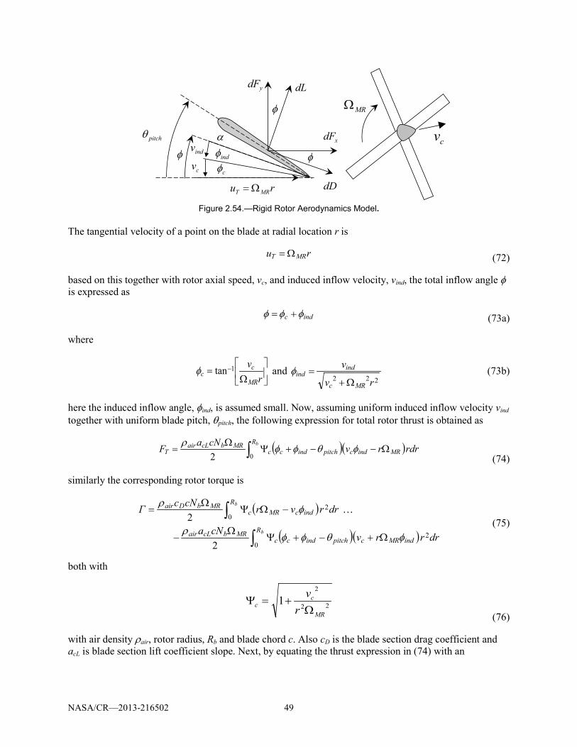
NASA/CR—2013-216502 49

Figure 2.54.—Rigid Rotor Aerodynamics Model.

The tangential velocity of a point on the blade at radial location r is

ru MRT Ω= (72)

based on this together with rotor axial speed, vc, and induced inflow velocity, vind, the total inflow angle φ is expressed as

indc φφφ += (73a)

where

Ω

= −

rvMR

cc

1tanφ and 222 rv

v

MRc

indind

Ω+=φ (73b)

here the induced inflow angle, φind, is assumed small. Now, assuming uniform induced inflow velocity vind together with uniform blade pitch, θpitch, the following expression for total rotor thrust is obtained as

( )( )rdrrvcNaF bR

MRindcpitchindccMRbcLair

T ∫ Ω−−+ΨΩ

=02

φθφφρ

(74)

similarly the corresponding rotor torque is

( )

( )( ) drrrvcNa

drrvrcNcΓ

b

b

RindMRcpitchindcc

MRbcLair

RindcMRc

MRbDair

20

20

2

2

∫

∫Ω+−+Ψ

Ω−

−ΩΨΩ

=

φθφφρ

φρ

(75)

both with

22

2

1MR

cc r

vΩ

+=Ψ (76)

with air density ρair, rotor radius, Rb and blade chord c. Also cD is the blade section drag coefficient and acL is blade section lift coefficient slope. Next, by equating the thrust expression in (74) with an

pitchθ

MRΩ

cv

ru MRT Ω=

cφindφα

φ indv

cvφ

φ

dL

dD

xdF

ydF

NASA/CR—2013-216502 50

expression based on momentum theory (Ref. 41), we obtain the following equation for the induced inflow ratio indλ

02 =++ λλλ λλ cba indind (77a)

with coefficients

241ln6ln48 2 −

++

= c

c

ccLc

c

c aa λλγσλ

λγ

λ (77b)

( ) σλσθλσγλλγσλ

λλ cLcpitchcLccLccc

ccLc

caaaab 36tan624ln61sin24 1231 −−+−+

+

= −− (77c)

( )cpitchcccL

cccLccccLcc

cpitchcL

a

aaac

λθγσγ

σλγλλσγλλγθπσλ

12

213

tan2

][tan21ln2

−

−

−+

−−

+−−=

(77d)

and with induced and forward speed inflow ratios

MRb

indind R

vΩ

=λ , MRb

cc R

vΩ

=λ and 21 cc λγ += (78)

and with rotor solidity ratio

b

b

RcNπ

σ = (79)

Based on Equations (77) to (79), the induced velocity, vind, is determined from the roots of Equation (77a). Using this result in Equations (74) to (75), the rotor thrust and torque values can be computed for a given rotor speed, forward speed and blade pitch angle as shown in the rotor thrust and torque simulation block in Figure 2.55. The rotor parameters used in the comprehensive simulations presented in Section 7.0 are summarized in Table 2.3 and Table 2.4.

Table 2.3 gives the main rotor parameters used in the single rotor helicopter simulation.

Figure 2.55.—Rotor thrust and torque simulation block.

indv

TF

Γ

pitchθ

cvMRΩ

Rotor

Model

NASA/CR—2013-216502 51

TABLE 2.3.—MAIN ROTOR PARAMETERS USED IN VARIABLE SPEED HELICOPTER SIMULATION

Parameter Value Rotor speed (high), ΩMR,high .......................................... 190 RPM Rotor speed (low), ΩMR,low ......................................... 102.5 RPM Number of blades, Nb .................................................................. 6 Rotor radius, Rb .................................................................. 11.5 m Rotor solidity, σ ................................................................... 0.115 Blade mass, mb ................................................................... 386 kg Rotor rotational inertia, JMR ............................... 4.054×104 kg m2 Section lift coefficient, cD .................................................... 0.012 Section drag coefficient, acL ................................................... 5.08

Table 2.4 gives the main rotor parameters used in the tiltrotor simulation.

TABLE 2.4.—MAIN ROTOR PARAMETERS USED IN VARIABLE SPEED TILTROTOR SIMULATION

Parameter Value Rotor speed (high), ΩMR,high ........................................... 190 RPM Rotor speed (low), ΩMR,low .......................................... 102.5 RPM Number of blades, Nb ................................................................. 4 Rotor radius, Rb ................................................................. 9.91 m Rotor solidity, σ .................................................................... 0.13 Blade mass, mb .................................................................. 372 kg Rotor rotational inertia, JMR ............................... 4.874×104 kg m2 Section lift coefficient, cD .................................................... 0.012 Section drag coefficient, acL ................................................ 5.056

2.6 Additional Information: Transformation Matrices Among Different Coordinate Frames

𝑇𝑓𝑟 = 𝑐𝑜𝑠(𝛽 + 𝛽0) 0 𝑠𝑖𝑛(𝛽 + 𝛽0)

0 1 0𝑠𝑖𝑛(𝛽 + 𝛽0) 0 𝑐𝑜𝑠(𝛽 + 𝛽0)

𝑇𝑙𝑓 = 𝑐𝑜𝑠𝜁 −𝑠𝑖𝑛𝜁 0𝑠𝑖𝑛𝜁 𝑠𝑖𝑛𝜁 0

0 0 1

𝑇𝑝𝑙 = 1 0 00 𝑐𝑜𝑠𝜃𝑝 𝑠𝑖𝑛𝜃𝑝0 −𝑠𝑖𝑛𝜃𝑝 𝑐𝑜𝑠𝜃𝑝

[𝑇𝑟𝑠] = −𝑐𝑜𝑠𝜓 𝑠𝑖𝑛𝜓 0𝑠𝑖𝑛𝜓 𝑐𝑜𝑠𝜓 0

0 0 1

𝑇𝑡𝑝𝑠 = 𝑐𝑜𝑠𝛽1𝑐 𝑠𝑖𝑛𝛽1𝑐𝑠𝑖𝑛𝛽1𝑠 𝑠𝑖𝑛𝛽1𝑐𝑐𝑜𝑠𝛽1𝑠

0 𝑐𝑜𝑠𝛽1𝑠 −𝑠𝑖𝑛𝛽1𝑠−𝑠𝑖𝑛𝛽1𝑐 𝑐𝑜𝑠𝛽1𝑐𝑠𝑖𝑛𝛽1𝑠 𝑐𝑜𝑠𝛽1𝑐𝑐𝑜𝑠𝛽1𝑠

NASA/CR—2013-216502 52

[𝑇] =

⎣⎢⎢⎢⎢⎡ 1 − 𝑣′2

2− 𝑤′2

2𝑣′ 𝑤′

−(𝑣′𝑐𝑜𝑠𝜃1 + 𝑤′𝑠𝑖𝑛𝜃1) 𝑐𝑜𝑠𝜃1 1 − 𝑣′2

2 − 𝑣′𝑤′𝑠𝑖𝑛𝜃1 𝑠𝑖𝑛𝜃1 1 − 𝑤′2

2

𝑣′𝑠𝑖𝑛𝜃1 − 𝑤′𝑐𝑜𝑠𝜃1 −𝑠𝑖𝑛𝜃1 1 − 𝑣′2

2 − 𝑣′𝑤′𝑐𝑜𝑠𝜃1 𝑐𝑜𝑠𝜃1 1 − 𝑤′2

2⎦⎥⎥⎥⎥⎤

NASA/CR—2013-216502 53

3.0 Driveshaft Subsystem 3.1 Introduction

Rotorcraft power transmission shafting is mounted within flexible structures such as the wings, tail, or fuselage, depending on the rotorcraft application. These structures naturally will deform under normal operation of the aircraft. To accommodate such motion, the shafting system is comprised of several shaft segments connected by flexible couplings, which are generally nonconstant velocity (NCV). A shaft system with misaligned NCV couplings gives rise to a phenomenon called Cardan error in which the motion of the input shaft is not perfectly matched by the output shaft; for example, if the two shafts are misaligned and the input shaft has a constant angular velocity, the velocity of the output shaft will fluctuate around the input speed. This Cardan error leads to some interesting dynamic phenomena. DeSmidt, et al., 2002, (Ref. 27) for example, shows that a static misalignment angle in the NCV coupling creates a coupling between the lateral and torsional vibration of the shaft system, leading to self-excited oscillations and even instability in some conditions. Similar parametric instability phenomena is also demonstrated by Mazzei and Scott, 2006, (Ref. 64).

3.2 Modeling

After many preliminary studies, a model was formulated which captured the essential features of a rotorcraft driveline mounted on a flexible support. Figure 3.1 depicts this model, which is based on a tiltrotor wing with a shaft running through.

Figure 3.2 shows a progression of modeling to help explain the final model. The left most figure shows a sketch of a typical tiltrotor aircraft, and we wish to model the wing structure and the cross-shafting, depicted in the middle pane. For clarity of analysis, the model is kept to a single shaft segment of length L coupled to the input shaft by a single NCV coupling, represented by a small circle between the two shafts. The torsionally flexible, laterally rigid shaft is connected to a lumped inertia, J0, at one end, representing a rotor load or the inertia of a shaft vibration mode. This shaft-inertia configuration, viewed as an inertia attached to a torsion bar with light torsional damping, has a torsional stiffness and damping given by kt and ct, respectively. The wing structure is modeled as a flexible cantilevered beam (represented by the blue rectangle in the middle figure) and is connected to the shaft by a rigid bearing, so the shaft and structure essentially move together. If the structure primarily moves in its first vibration mode, then it can be assumed as an equivalent mass-spring-damper oscillator coupled to the shaft as shown in the right part of Figure 3.2. Here, the lateral inertia of the support structure, shafting, and rotor are all lumped together as the parameter I0. The stiffness and damping of the structure are modeled as lumped elements kb and cb, respectively. )(ˆ tTL and )(ˆ tFL represent arbitrary torsional and lateral forcing, for example, from aerodynamic loading.

Figure 3.1.—Schematic of the model of a shaft system

mounted on a flexible support.

NASA/CR—2013-216502 54

Figure 3.2.—Progression in modeling from a tiltrotor aircraft to the current model. Black boxes represent ground and

the blue rectangle of the middle pane represents a flexible support structure.

The lateral motion of the shaft pivoting about the NCV coupling is given by α(t), which is a degree of freedom. The motion is assumed to be planar since a wing structure is generally less stiff in the vertical direction than in the fore-aft direction. The misalignment of the shaft is permitted to vary dynamically, which more realistically represents the system dynamics than a static misalignment angle. The input shaft has a prescribed motion, φ0(t), and as discussed before, the output motion of the NCV coupling does not match the input if misalignment is present. The angular motion directly after the NCV coupling is φ1(α(t), φ0(t)). The motion of the inertia J0 is then given by φ1+φe(t), where φe(t) is the elastic motion of the inertia and is the second degree of freedom of the system.

The motion φ1 can be determined using geometric arguments as in Martin, 1969, (Ref. 65). For planar misalignment,

αφφ cos

tantan

1

0 = (1)

Note that this is a kinematic constraint relating φ1 and α, so it can be solved for φ1 and later it will replace all instances of φ1 in the equations of motion, leaving just the prescribed parameter φ0 and the degree of freedom α.

Now the equations of motion can be derived by formulating the energies and applying Lagrange’s Equations. The kinetic and potential energies are given, respectively, by,

202

12102

1 )( αφφ

IJT e ++= (2)

2212

21 )( αφ LkkV bet += (3)

A Rayleigh dissipation function can also be written to account for damping,

2212

21 )( αφ

LccD bet += (4)

Applying Lagrange’s Equations,

qQqD

qV

qT

qT

dtd

=∂∂

+∂∂

+∂∂

−

∂∂

(5)

where q represents either φe or α and Qq represents the corresponding external loading, either LT and

LFL ˆ , respectively, the equations of motion become

Letette T=+++ 122 φφωφξωφ (6a)

Lebbb Fg =+++ ),,,(2 1112 φφφφηαωαξωα

(6b)

NASA/CR—2013-216502 55

Here, the following new parameters have been defined:

000

0

000

22

0

2ˆ

,ˆ

,,2

,2

,,IFLF

JTT

IJ

Ic

Jc

ILk

Jk L

LLb

bb

t

tt

bb

tt ======= η

ωξ

ωξωω (7)

Also, the function g represents a complicated expression.

3.3 Analysis

At this point, one can apply the constraint Equation (1) to the equations of motion (6). For the purposes of analysis, the terms in these nonlinear equations can be expanded in a Taylor series over the degree of freedom α around α = 0, the equilibrium position of the lateral motion of the shaft. The trigonometric functions are also converted to exponentials.

Now, the method of multiple scales (MMS), Nayfeh and Mook, 1979 (Ref. 66), a nonlinear solution technique, can be applied to the equations of motion. MMS provides a way to find the approximate solution of a set of nonlinear equations by using multiple time scales as independent variables; mathematically:

,, , 2210 tTtTtT εε === (8)

where ε is a small parameter. Then time derivatives become ordered in the small parameter:

++=+∂∂

+∂∂

= 101

1

0

0 DDTdt

dTTdt

dTdtd ε (9a)

++= 10202

22 DDD

dtd ε (9b)

Additionally, express the solutions φe(t) and α(t) as straightforward expansions, neglecting terms of O(ε3) and higher:

),(),();( 1022

101 TTTTte ϕεεϕεφ += (10a)

),(),();( 1022

101 TTTTt αεεαεα += (10b)

Also, the analysis will assume light damping of O(ε1):

bbbttt εµξωεµξω == , (11)

Applying Equations (8) to (11) to Equations (6), considering the external forcing functions to be O(ε1), and collecting terms of like orders of ε (as is typical for MMS) gives the ordered equations of motion. Equations of O(ε1) and O(ε2) are presented here:

O(ε1):

Lt TD =+ 12

120 ϕωϕ (12a)

( ) Lii

b FeeiD =−++ −10

221

21

20 00

4αφηαωα φφ (12b)

NASA/CR—2013-216502 56

O(ε2):

( )( )

( ) ( ))()(2

)(22

12012

12102

120

21

22

0214

10101

22101102

22

20

00

00

αααφα

φαφααϕµϕϕωϕ

φφ

φφ

DDeei

DeeDDDD

ii

iitt

++−−−

+−−−−=+

−

−

(13a)

( ) ( ) 1122

101102022

22

220 0000

422

4ϕαηαµααφηαωα φφφφ ii

bii

b eeiDDDeeiD −−−−=−++ −− (13b)

Here, i represents the imaginary unit. At this point, the motion of the input shaft φ0 is still arbitrary. One reasonable choice for motion is a constant angular velocity described as:

0,, 00000 =Ω=Ω= φφφ t (14)

Letting the external forcing go to zero, the solution to the O(ε1) Equations (12) is:

00 )()(),( 1111101TiTi tt eTPeTPTT ωωϕ −+= (15a)

00 )()(),( 1111101TiTi bb eTAeTATT ωωα −+= (15b)

Now Equations (14) and (15) can be used to fully define the right hand sides of the O(ε2) equations, (13). After this substitution, it becomes clear that terms on the right hand side are secular for certain values of the input shaft speed Ω0 (rad/sec) in other words, these terms cause resonance in the O(ε2) equations. This would mean that the higher order corrections to the solution grow quite large as time progresses, which makes the expansion not uniformly valid. The general procedure for dealing with these secular terms is to set them to zero, which provides conditions for finding the functions P1 and A1.

When the shaft takes one of the following values, a secondary resonance occurs:

10 2 tΩ = ω (16a)

10 2 t bΩ = −ω ω (16b)

10 2 t bΩ = +ω ω (16c)

10 2 t bΩ = − +ω ω (16d)

Comparing with Nayfeh and Mook, 1979, (Ref. 66), these secondary resonance conditions appear to be cases for internal resonance, in which the two degrees of freedom become coupled nonlinearly, though linearly, they are uncoupled.

3.4 Significance

The conditions found in the previous section are the result of some interesting analysis, but it must also be shown that they have practical implications as well. The goal of this section is to find the natural frequencies of the driveline and foundation system in order to show that the shaft speed may coincide with one of the conditions in Equations (16). In this section, ball park values for the parameters of a more realistic shaft system will be estimated based on preliminary design data for the LCTR2 large civil tiltrotor concept (for example, Acree and Johnson, 2008, (Ref. 67)).

NASA/CR—2013-216502 57

Based on internal discussions, it was decided to design a driveline for the scenario of a large tiltrotor with a total of four engines, one of them being disabled. This shafting should transmit 3750 HP, which is half of the power of an engine at full power. The shaft was designed to run at 7000 RPM, nearly the same as the cross-shafting of a CH-47, which is also a fairly large and powerful aircraft. The shaft uses aluminum material properties.

The cases of torsional buckling and yielding were investigated as the two failure scenarios. These cases were evaluated using maximum shear stress theory and the buckling equations of Shokrieh, et al., 2004, (Ref. 68). Total driveline length was estimated from Acree and Johnson, 2008, at 65 ft and the cases of 6 and 8 driveshaft segments were investigated. Using these constraints and reasonable estimates of dimensions and factors of safety (approximately 4), a potential shaft was sized with a wall thickness of 0.118 in. and outer radius of 3.14 in. The stiffness can be calculated by using the equation of a rod in torsion, as in Rao, 2004, (Ref. 69), for instance:

( )4432

dDLGk

DLt −=

π (17)

where G is shear modulus, LDL is the driveline length, and D and d are the outer and inner shaft diameters, respectively. Then the stiffness is 12300 Nm. The shaft properties and dimensions are summarized in Table 3.1.

TABLE 3.1.—SHAFT PROPERTIES AND DIMENSIONS Shaft property Value Power transmitted, Ptr ...................................................... 3750 HP Design shaft speed, Ωn .................................................. 7000 RPM Material ......................................................................... Aluminum Yield stress, Sy .................................................................. 270 MPa Young’s modulus, E ........................................................... 70 GPa Shear modulus, G ............................................................... 27 GPa Mass density, ρ ............................................................. 2710 kg/m3

Driveline length, LDL ............................................................... 65 ft Wall thickness, t ............................................................... 0.118 in. Outer radius, ro ................................................................... 3.14 in. Torsional stiffness, kt ..................................................... 12300 Nm

Now the inertia properties of the rotor must be estimated. From Acree and Johnson, 2008, the mass of

both rotor disks for the LCTR2 is 8756 lb. The individual rotor blade mass, accounting for the mass of the hub, is estimated as one tenth of this value, or 876 lb. Knowing the diameter of the rotor disk (drotor = 65 ft) from Acree and Johnson, 2008 and estimating the blade as a slender rod rotating about its end, one can compute the estimated rotor inertia as 52000 kg-m2.

Due to the gearbox between the shafting and the rotor, the shafting will “see” a different inertia than this depending on the gear ratio. Acree and Johnson, 2008 give blade tip velocities for the cases of cruise and hover, vtc = 650 ft/s and vth = 400 ft/s, respectively. Using the blade length, one can determine the angular velocity of the rotor disk in cruise and hover, and knowing the shaft speed, the gear ratios for each case can be determined. The gearing makes the rotor inertia easier to turn from the point of view of the shaft, so the effective rotor inertias for hover and cruise, respectively, are Jeff,h = 1420 kg-m2 and Jeff,c = 877 kg-m2.

Using the estimated effective inertias and the shaft stiffness, now the torsional natural frequency of the driveline-rotor system can also be estimated assuming it behaves as a shaft pinned on one end and attached to an inertia (the rotor) at the other. For cruise and hover, these turn out to be ωt,c = 3.75 rad/s and ωt,h = 2.95 rad/s.

From Acree and Johnson, 2008, the first lateral bending natural frequencies of the LCTR2 wing structure is about fb = 2.3 Hz or ωb = 14.5 rad/s. Now, the shaft operates nominally at 7000 RPM = 735

NASA/CR—2013-216502 58

rad/s. In view of Equations (16), the shaft speed will not coincide with a secondary resonance condition under a normal speed shift between hover and cruise.

Considering higher modes of vibration could lead to such a coincidence though. The rotor inertia is quite large compared with the torsional inertia of the shaft, so treat the shaft as a pin-pin distributed parameter torsion rod. By Rao, 2004, (Ref. 69), natural frequencies of the rod are given by

,...3,2,1,, == nGLn

LDnt ρ

πω (18)

The first natural frequency is given by ωt,1 = 1001 rad/s. In view of Equations (16), during a 50 percent speed decrease, taking the shaft speed to 3500 RPM, or 368 rad/s, the shaft speed will cross secondary resonances at Ω0b = 486 rad/s, Ω0a = 500 rad/s , Ω0c = 515 rad/s. So in this example, the first shaft torsional mode of vibration and the first lateral bending mode of the foundation have natural frequencies which allow Equations (16) to be satisfied, and these secondary resonances could be cause for concern during aircraft flight. These conditions will be investigated further in the next section.

3.5 Constant Speed Operation Results

Operating at these secondary resonances leads to phenomena which are not accounted for in linear analysis, so these scenarios could be important in the design of variable speed rotorcraft. If large vibrations are involved when the input shaft speed passes through one of these secondary resonances, then they should be considered and treated with care by designers, just as linear resonances play a role in aircraft design. It makes sense to first explore these conditions at constant speed operation to get an idea of how they behave before performing variable speed simulations.

These secondary resonance conditions were found via some simplifications of the original nonlinear equations of motion (6), for example, using the Taylor expansion. It is prudent to run some simulations of the system using the full nonlinear NCV joint constraint, (1). For simulation, (1) is put into a slightly different form, solving for φ1 directly:

][tantancostantan 0

10

011 φφ

αφφ −− −+

= (19)

The first term on the right hand side provides for the fluctuation of the motion when misalignment is present, and the second and third terms on the right hand side guarantee that the angle φ1 steadily increases as φ0 steadily increases.

Now Equations (6) and (19) can be numerically integrated to determine solutions of the system dynamics. To clearly showcase the phenomenology, convenient parameters will be chosen for initial simulations, taking care to keep the phenomena of these secondary resonance speeds from overlapping. In the following simulations, the external forcing will be set to zero, so these will be free responses of a parametrically excited system. This is done to avoid any confusion between effects produced by the oscillation of system and effects due to the external forcing.

For comparison with subsequent examples, Figure 3.3 shows an example of the shaft system in free vibration with the input shaft speed set away from any of the conditions in Equations (16). The parameter set used for this simulation is ωt = 100 rad/s, ωb = 30 rad/s, Ω0 = 85 rad/s, η = 0.5, ζt = ζb = 0, along with initial conditions γ0 = 0.1 rad, and α0 = 0.01 rad in the torsional and lateral directions, respectively. The result is quite similar to two uncoupled, linear oscillators in free vibration. The left pane shows a very dense vibration signal, which is typical of subsequent simulations; for clarity, a zoom-in of the first 2 sec of the response is given in the right pane.

The remainder of this section will present and discuss three examples of simulations under the conditions of (16).

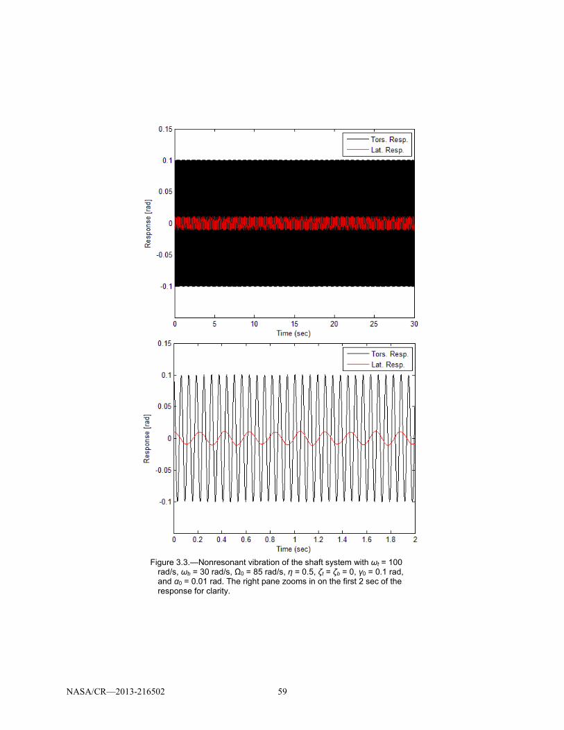
NASA/CR—2013-216502 59

Figure 3.3.—Nonresonant vibration of the shaft system with ωt = 100

rad/s, ωb = 30 rad/s, Ω0 = 85 rad/s, η = 0.5, ζt = ζb = 0, γ0 = 0.1 rad, and α0 = 0.01 rad. The right pane zooms in on the first 2 sec of the response for clarity.

NASA/CR—2013-216502 60

Figure 3.4.—System response (internal resonance) to the condition

given in Equation (16d) with ωt = 100 rad/s, ωb = 90 rad/s, Ω0 = 40 rad/s, η = 1.2, γ0 = 0.1 rad, and α0 = 0.01 rad.

3.5.1 Case 1 Figure 3.4 shows an example of operating the system under the condition given by (16d). In this case,

ωt = 100 rad/s, ωb = 90 rad/s, Ω0 = 40 rad/s, and η = 1.2, and the system is given in initial conditions of γ0 = 0.1 rad and α0 = 0.01 rad in the torsional and lateral directions, respectively. This would correspond to an initial twist in the shaft of about 6° and NCV joint misalignment of about 0.6°. Also, damping is set to zero. The response is an internal resonance characterized by strong coupling between coordinates that are linearly uncoupled. One can see that the larger amplitude torsional vibration drives the lateral vibration from a small value to a large one.

Looking at the vibration energy in the system over time sheds some more light on this nonlinear coupling behavior. Mass specific energy in the torsional (Etors) and lateral (Elat) directions, as well as the total specific energy (Etot) in the system, can be computed by:

22212

21 αωα ttorstorstors PEKEE +=+= (20a)

22212

21

ebelatlatlat PEKEE φωφ +=+= (20b)

lattorslot EEE += (20c)

These energies are plotted over time in Figure 3.5 for the same scenario as in Figure 3.4. As expected, the nonlinear coupling leads to an energy exchange between the torsional and lateral motion. An upshot of this is that if the frequency condition is satisfied, then the system could experience motion beyond what it was designed to handle, leading to increased fatigue or possibly to outright fracture.

In addition, the total energy in the system is fluctuating over time. There is no external forcing on the system, only the variation in the parameters caused by the NCV coupling. More energy coming into the system could, again, lead to high vibration amplitudes.

Changing the value of the inertia ratio η also has effects on the system response. Increasing to η = 3.3 leads to an increase in the nonlinearity of the system. Figure 3.6 shows that the frequency of the energy exchange between modes also increases, as does the amplitude of the lateral vibration. Increasing further

NASA/CR—2013-216502 61

to η = 5.0, shown in Figure 3.7, causes the response to become chaotic. Also, the maximum amplitude of the lateral vibration has increased further. This chaotic vibration is qualitatively different than the internal resonance, but essentially, the potential harmful effects on the system (large vibrations) are the same.

Adding a small amount of damping to the system can cause this motion to decay, at least in the case of free response under current investigation. Equal lateral and torsional damping of ζt = ζb = 0.01 is set in the system. If the system is linearized, this would correspond to 1 percent critical damping.

The results of adding damping are shown in Figure 3.8. In the top pane, the damping effectively causes the motion to decay, preventing any large vibrations for the choice of system parameters and initial conditions defined for the previous figure. Increasing the initial conditions to γ0 = 0.2 rad, and α0 = 0.1 rad, as in the bottom pane of Figure 3.8, still allows for a substantial growth in the lateral motion of the shaft system before the damping takes over and causes the response to die away. Damping could be an effective way to deal with this type of response, though it should be chosen judiciously in order to ensure a limited vibration response.

As a note, the condition Equation (16b) has behavior similar to (16d), so the investigation of (16b) need not be presented here.

Figure 3.5.—Vibration energy in the shaft system with ωt = 100 rad/s, ωb = 90 rad/s, Ω0 = 40 rad/s, η = 1.2, γ0 = 0.1 rad, and α0 = 0.01 rad.

NASA/CR—2013-216502 62

Figure 3.6.—System response (internal resonance transitioning

to chaotic vibration) to the condition given in Equation (16d) with ωt = 100 rad/s, ωb = 90 rad/s, Ω0 = 40 rad/s, η = 3.3, γ0 = 0.1 rad, and α0 = 0.01 rad.

Figure 3.7.—System response (chaotic vibration) to the condition

given in Equation (16d) with ωt = 100 rad/s, ωb = 90 rad/s, Ω0 = 40 rad/s, η = 5.0, γ0 = 0.1 rad, and α0 = 0.01 rad.

NASA/CR—2013-216502 63

Figure 3.8.—System response to the condition given in Equation (16d)

with ωt = 100 rad/s, ωb = 90 rad/s, Ω0 = 40 rad/s, η = 5.0, and ζt = ζb = 0.01. Initial conditions for the top pane are γ0 = 0.1 rad and α0 = 0.01 rad, and for the bottom pane are γ0 = 0.2 rad and α0 = 0.1 rad.

NASA/CR—2013-216502 64

Figure 3.9.—System response to the condition given in Equation (16c)

with ωt = 100 rad/s, ωb = 30 rad/s, Ω0 = 80 rad/s, η = 0.5, γ0 = 0.1 rad, and α0 = 0.01 rad. Top panel shows zero damping, while the bottom panel includes damping (ζt = ζb = 0.02).

3.5.2 Case 2 The condition (16c) is investigated next. Values for the system parameters are set at ωt = 100 rad/s,

ωb = 30 rad/s, Ω0 = 80 rad/s, and η = 0.5. The initial conditions are the same as the previous example, letting γ0 = 0.1 rad and α0 = 0.01 rad in the torsional and lateral directions, respectively. The result for zero damping is given in the top panel of Figure 3.9, which shows a rather severe instability. Clearly, this is a worrisome situation during shaft operation. Adding some damping (ζt = ζb = 0.02, or 2 percent critical

NASA/CR—2013-216502 65

of the linearized system) to the system counteracts this instability quite effectively for this parameter set, as shown in the bottom panel of Figure 3.9.

Increasing the inertia ratio requires an increase in the damping level to counteract the instability. In Figure 3.10, the inertia ratio has been increased to η = 0.5. In the top panel, the lateral damping is ζb = 0.03, and this level of damping keeps the response from growing unbounded, but the response does reach a fairly high steady state amplitude of about 0.4 rad or 23°. The bottom panel shows that a much higher amount of lateral damping, ζb = 0.12, is necessary to cause the vibration to decay. These results show that large amplitude can be realized at this shaft speed, but that an appropriate choice of damping may be able to limit the vibrations.

Figure 3.10.—System response to the condition given in Equation (16c)

with ωt = 100 rad/s, ωb = 30 rad/s, Ω0 = 80 rad/s, η = 0.5, ζt = 0.02, ζb = 0, γ0 = 0.1 rad, and α0 = 0.01 rad. In the top panel, ζb = 0.03, while in the bottom panel, ζb = 0.12.

NASA/CR—2013-216502 66

3.5.3 Case 3 Now condition (16a) is investigated with the parameter choices ωt = 100 rad/s, ωb = 30 rad/s, Ω0 = 50

rad/s, and η = 0.5. In Figure 3.11, applying zero damping and initial conditions γ0 = 0.1 rad, and α0 = 0.01 rad, it appears that nothing interesting is happening here, and even that the motion in the torsional direction may be decaying.

Increasing the lateral initial condition to α0 = 0.03 rad reveals that the torsional response at this shaft speed first decreases and then grows unstable, as displayed in the top pane of Figure 3.12. The bottom pane shows that decreasing the torsional initial condition to γ0 = 0.01 rad actually results in a larger response sooner in time. It is also noted that these adjustments have negligible effects on the lateral response. Also, many simulations (not shown here for brevity) indicate that the inertia ratio η has essentially no effect on the response of the system. As can be observed in the equations of motion (6), η only effects the lateral dynamics. Since the instability occurs in the torsional dynamics, this result makes sense.

Adding a small amount of damping (ζt = ζb = 0.01) to the system stabilizes the system quite readily, even for somewhat large initial conditions (γ0 = 0.1 rad, and α0 = 0.1 rad), as presented in Figure 3.13. Other choices for initial conditions yield the same qualitative behavior. Simulations indicate that for realistic values of damping and vibrations, the condition (16a) may not present problems for shaft operation, though behavior for zero damping is noted.

Figure 3.11.—System response to the condition given in Equation (16a) with ωt = 100 rad/s, ωb = 30 rad/s, Ω0 = 50 rad/s, η = 0.5, ζt = ζb = 0, γ0 = 0.1 rad, and α0 = 0.01 rad.

NASA/CR—2013-216502 67

Figure 3.12.—System response to the condition given in (Eq. (16a))

with ωt = 100 rad/s, ωb = 30 rad/s, Ω0 = 50 rad/s, η = 0.5, ζt = ζb = 0, and α0 = 0.03 rad. In the top pane, γ0 = 0.1 rad and in the bottom pane, γ0 = 0.01 rad.

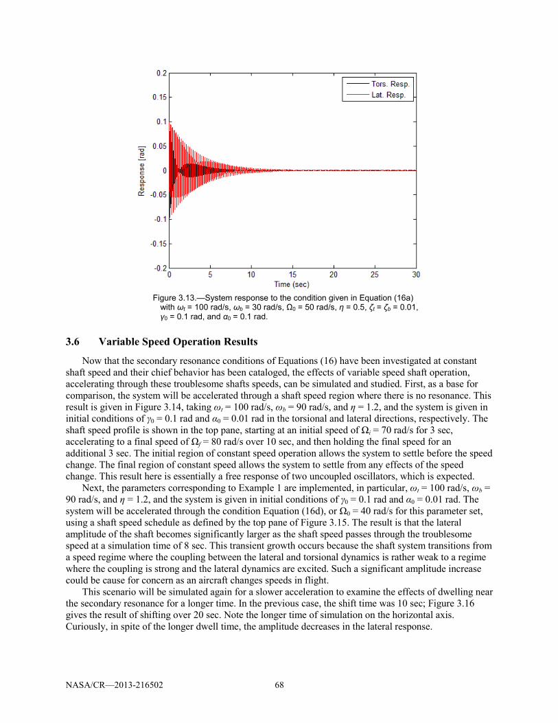
NASA/CR—2013-216502 68

Figure 3.13.—System response to the condition given in Equation (16a)

with ωt = 100 rad/s, ωb = 30 rad/s, Ω0 = 50 rad/s, η = 0.5, ζt = ζb = 0.01, γ0 = 0.1 rad, and α0 = 0.1 rad.

3.6 Variable Speed Operation Results

Now that the secondary resonance conditions of Equations (16) have been investigated at constant shaft speed and their chief behavior has been cataloged, the effects of variable speed shaft operation, accelerating through these troublesome shafts speeds, can be simulated and studied. First, as a base for comparison, the system will be accelerated through a shaft speed region where there is no resonance. This result is given in Figure 3.14, taking ωt = 100 rad/s, ωb = 90 rad/s, and η = 1.2, and the system is given in initial conditions of γ0 = 0.1 rad and α0 = 0.01 rad in the torsional and lateral directions, respectively. The shaft speed profile is shown in the top pane, starting at an initial speed of Ωi = 70 rad/s for 3 sec, accelerating to a final speed of Ωf = 80 rad/s over 10 sec, and then holding the final speed for an additional 3 sec. The initial region of constant speed operation allows the system to settle before the speed change. The final region of constant speed allows the system to settle from any effects of the speed change. This result here is essentially a free response of two uncoupled oscillators, which is expected.

Next, the parameters corresponding to Example 1 are implemented, in particular, ωt = 100 rad/s, ωb = 90 rad/s, and η = 1.2, and the system is given in initial conditions of γ0 = 0.1 rad and α0 = 0.01 rad. The system will be accelerated through the condition Equation (16d), or Ω0 = 40 rad/s for this parameter set, using a shaft speed schedule as defined by the top pane of Figure 3.15. The result is that the lateral amplitude of the shaft becomes significantly larger as the shaft speed passes through the troublesome speed at a simulation time of 8 sec. This transient growth occurs because the shaft system transitions from a speed regime where the coupling between the lateral and torsional dynamics is rather weak to a regime where the coupling is strong and the lateral dynamics are excited. Such a significant amplitude increase could be cause for concern as an aircraft changes speeds in flight.

This scenario will be simulated again for a slower acceleration to examine the effects of dwelling near the secondary resonance for a longer time. In the previous case, the shift time was 10 sec; Figure 3.16 gives the result of shifting over 20 sec. Note the longer time of simulation on the horizontal axis. Curiously, in spite of the longer dwell time, the amplitude decreases in the lateral response.

NASA/CR—2013-216502 69

Figure 3.14.—System response to a variable speed input with ωt = 100 rad/s, ωb = 90 rad/s, η = 1.2, γ0 = 0.1 rad, α0 = 0.01 rad, Ωi = 70 rad/s, and Ωf = 80 rad/s.

NASA/CR—2013-216502 70

Figure 3.15.—Accelerate the shaft through the speed condition Equation (16d)

in 10 sec. Parameters are ωt = 100 rad/s, ωb = 90 rad/s, η = 1.2, γ0 = 0.1 rad, α0 = 0.01 rad, Ωi = 35 rad/s, and Ωf = 45 rad/s.

NASA/CR—2013-216502 71

Figure 3.16.—Accelerate the shaft through the speed condition Equation (16d)

in 20 sec. Parameters are ωt = 100 rad/s, ωb = 90 rad/s, η = 1.2, γ0 = 0.1 rad, α0 = 0.01 rad, Ωi = 35 rad/s, and Ωf = 45 rad/s.

This can be explained by another simulation given in Figure 3.17. The only change in this simulation

is to extend the time of constant speed operation at the beginning of the simulation by 1 sec from 3 sec in Figure 3.16 to 4 sec in Figure 3.17. As the system transitions through this secondary resonance regime, a big factor in the amplitude of the motion is the “initial condition” of the response as the shaft speed approaches a secondary resonance condition. If, in the course of oscillation, the motion is nearly zero as the condition is approached, then the amplitude will naturally be small as in Figure 3.16, since in a nonlinear system, small amplitudes of vibrations don’t engage the nonlinear effects very much.

NASA/CR—2013-216502 72

On the other hand, if the oscillation is relatively large as the shaft speed approaches the secondary resonance condition, the motion has the potential to grow large, as in Figure 3.17. In addition, the lateral response is larger than in Figure 3.15, confirming that a longer dwell time also can lead to a larger response.

Accelerating the shaft through the secondary resonance condition given by Equation (16a) does not lead to any notable results. Responses typically look like those in Figure 3.14. This instability grows much more slowly in amplitude than the growth produced by the other conditions, so it follows that the response would not grow much by passing through this speed.

Figure 3.17.—Accelerate the shaft through the speed condition Equation (16d) in

20 sec. Parameters are ωt = 100 rad/s, ωb = 90 rad/s, η = 1.2, γ0 = 0.1 rad, α0 = 0.01 rad, Ωi = 35 rad/s, and Ωf = 45 rad/s. The only change from the results of Figure 3.16 is to extend the initial constant speed of constant speed operation by 1 sec.

NASA/CR—2013-216502 73

Accelerating the shaft through the other conditions in Equations (16) give qualitatively similar results; an amplitude change which depends on oscillation amplitude as the shaft speed approaches the secondary resonance and also a dependence on dwell time near the speed of secondary resonance.

Effects of damping on variable speed operation were not presented here. Since these simulations are free vibration, the damping would only lead to a decrease in amplitude as the shaft speed approaches a secondary resonance. At that point, it is equivalent to simply starting the system at constant, but lower, amplitude.

3.7 Conclusions

Due to the secondary resonances brought on by the nonlinearity of the flexible couplings, large vibrations could arise in the shaft system. Since in variable speed operation, the shaft may undergo speed changes over a wide range, it makes sense to consider this nonlinearity in the design of variable speed aircraft. The nonlinear modeling and analysis allows one to find these shaft speeds that may cause problems. Selecting an appropriate amount of damping and choosing a proper speed schedule for performing a rotor speed shift are two possible strategies for minimizing shaft vibration levels.

To further this investigation, more in-depth nonlinear analysis possibly could be performed to support the existence of internal resonance, chaotic vibration, and instability. More analysis may lead to closed form or semi-closed form ways to determine what parameter values cause transition from internal resonance to chaotic vibration and what values of damping are needed to subdue effects of operating near a secondary resonance condition. More realistic modeling, such as implementing a distributed parameter flexible foundation or using multiple shafts and NCV couplings, would add fidelity to the results. Free vibration of the system, as is studied here, is great for an initial study, but is not very realistic in terms of an aircraft operating in the real world; realistic external loading should be incorporated. Adding some unbalance to the shaft or rotor would also generate some interesting results, as one could compare the effects of operating near an ordinary linear resonance to operating near a nonlinear secondary resonance.

NASA/CR—2013-216502 74

4.0 Gas Turbine Engine Modeling 4.1 Introduction

In order to simulate the variable speed operation of the rotorcraft driveline, a transient gas turbine engine model has been developed. In general the gas turbine will undergo transient operations due to startups, changing loads, and sudden shutdowns. Here the main focus is to capture the effects due to sudden load changes which will be encountered during gear changes.

In the area of transient gas turbine engine modeling several researchers have explored techniques based on linearization models about the nominal operating conditions. Here the model Jacobian is estimated and the engine response about the nominal is computed (Refs. 70 and 71). However, such approaches are not valid for significant deviations about nominal which could be expected during severe or sudden operational load changes. More recently engine models based on the full nonlinear aero-thermal relations have been developed (Refs. 72 to 78). In these models, the nonlinear aero-thermal equations have been solved using various Newton-Raphson based methods. Such iterative solving procedures have been further explored by (Ref. 79) where it was found that the iterative nature was problematic for real-time simulations due to slow converges times. To address this, others have proposed non-iterative simulations techniques based on forward substitution methods (Ref. 80). Still others have utilized simplified compressor and turbine models which do not rely on engine maps allowing explicit solutions without the need for iteration at the expense of reduced simulation fidelity (Ref. 81).

The gas turbine engine model developed in this investigation is a nonlinear mechanical-aero-thermal model with lumped representation of the gas turbine components. The solution approach is based on non-iterative forward substitution similar to (Ref. 80) together with a new analytical method to explicitly compute the compressor and turbine performance maps. One key feature for a transient model is that the mass flow through each component is not necessarily the same. For example, at any instant the compressor and turbine could induce different mass flows depending on the instantaneous upstream and downstream pressures across each component. To account for this plenum chamber elements are included between each component to accommodate these transient differential mass flows and density changes. The mechanical-aero-thermal equations are implemented in the Matlab Simulink environment for use as a module in the comprehensive variable speed drive system simulation.

4.2 Transient Gas Turbine Engine Model

To simulate the effect of the engine and fuel control system dynamics during variable speed rotor operation, a generic twin spool gas turbine model is developed. The components of this model are shown in Figure 4.1. The components included in this analytical model are axial compressor, combustor, gas-generator turbine, power turbine and two mass accumulators (plenums). The torque balances between the compressor and gas generator turbine as well as between the power turbine and the load have also been included and the physical and thermodynamic laws (Ref. 75) have been utilized to describe the system dynamics. This analytical model is then implemented in the MATLAB/Simulink environment. The thermodynamic model is based on the standard idealized Joule/Brayton cycle (Ref. 70). The main assumptions made in this analytical model can be summarized as follows:

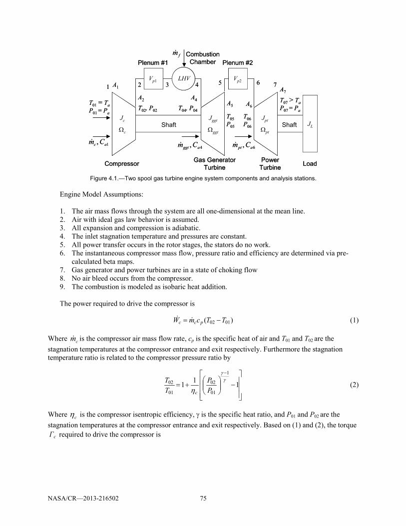
NASA/CR—2013-216502 75

Figure 4.1.—Two spool gas turbine engine system components and analysis stations.

Engine Model Assumptions: 1. The air mass flows through the system are all one-dimensional at the mean line. 2. Air with ideal gas law behavior is assumed. 3. All expansion and compression is adiabatic. 4. The inlet stagnation temperature and pressures are constant. 5. All power transfer occurs in the rotor stages, the stators do no work. 6. The instantaneous compressor mass flow, pressure ratio and efficiency are determined via pre-

calculated beta maps. 7. Gas generator and power turbines are in a state of choking flow 8. No air bleed occurs from the compressor. 9. The combustion is modeled as isobaric heat addition.

The power required to drive the compressor is

)( 0102 TTcmW pcc −= (1)

Where cm is the compressor air mass flow rate, cp is the specific heat of air and T01 and T02 are the stagnation temperatures at the compressor entrance and exit respectively. Furthermore the stagnation temperature ratio is related to the compressor pressure ratio by

−

+=

−

111

1

01

02

01

02 γγ

η PP

TT

c (2)

Where cη is the compressor isentropic efficiency, γ is the specific heat ratio, and P01 and P02 are the stagnation temperatures at the compressor entrance and exit respectively. Based on (1) and (2), the torque

cΓ required to drive the compressor is

Compressor

Shaft

Gas GeneratorTurbine

PowerTurbine Load

CombustionChamberPlenum #1 Plenum #2

1 2 3 4 5 6 7

1 , ac Cm

A1

A2 A4 A5

Shaft

A6

A7

Jggt JL

fm

T05P05

T06P06

T07 > TaP07 = Pa

T01 = TaP01 = Pa

4 , aggt Cm 6 , apt Cm

LHVVp1 Vp2

Ωggt

Jpt

Ωpt

Jc

Ωc

T02, P02 T04, P04

Compressor

Shaft

Gas GeneratorTurbine

PowerTurbine Load

CombustionChamberPlenum #1 Plenum #2

1 2 3 4 5 6 7

1 , ac Cm

A1

A2 A4 A5

Shaft

A6

A7

Jggt JL

fm

T05P05

T06P06

T07 > TaP07 = Pa

T01 = TaP01 = Pa

4 , aggt Cm 6 , apt Cm

LHVVp1 Vp2

Ωggt

Jpt

Ωpt

Jc

Ωc

T02, P02 T04, P04

NASA/CR—2013-216502 76

−

Ω

+Ω=

−

1

1

01

0201 γγ

η PPTcmJΓ

ccpcccc

(3)

Where Ωc is the compressor rotation speed and Jc is the compressor rotational inertia. Also, in the above equations the stagnation temperature and pressures at the compressor entrance are assumed to be the ambient atmospheric pressure, P01=Pa, and temperature T01 = Ta values. Furthermore compressor pressure ratio, 0102 / PPc =π , and efficiency, cη , are related to cm and Ωc the via the compressor characteristic maps,

),,,( 0101 cccPc mPTf Ω= π and ),,,( 0101 cccc mPTf Ω= ηη (4)

In this study, the compressor pressure and efficiency maps are generated numerically based on the nominal compressor design values as detailed in Section 4.3.

Furthermore, the compressor mass flow rate, cm , pressure ratio, πc, and efficiency characteristics, cη , are computed by way of so-called beta maps with functional dependencies,

),,,( ccaamc PTfm βΩ= and ),,,(

),,,(

ccaac

ccaaprc

PTf

PTf

βη

βπ

η Ω=

Ω=

(5a)

Where βc is the compressor beta parameter which maps the mass flow to pressure ratio as

2

ccc mβπ = (5b)

In this study, the compressor pressure and efficiency maps are generated numerically based on the nominal compressor design values (see Section 4.5).

To drive the compressor and load, separate gas generator and power turbines are present in the two-spool gas turbine engine (Figure 4.1). The power generated from these turbines is

)( 0504 TTcmW pggtggt −= and )( 0706 TTcmW pptpt −= (6)

Where ggtm and ptm are gas generator and power turbine mass flows, respectively, and T04, T05, T06 and T07 are turbine entrance and exit stagnation temperatures as defined in Figure 4.1. Furthermore, the turbine pressure ratios based on isentropic expansion thought the turbines are

1

05

04

05

04 −

=

γγ

TT

PP and

1

07

06

07

06 −

=

γγ

TT

PP (7)

and the turbine mass flows are computed based on the assumption that both turbines are operating in the condition of choking flow. Therefore

04

044

TPAmggt ϕ= and

06

066

TPAmpt ϕ= (8a)

with

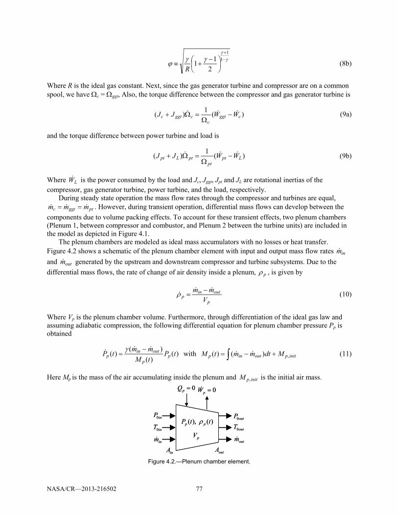
NASA/CR—2013-216502 77

γ

γγγϕ

−+

−+≡

11

211

R (8b)

Where R is the ideal gas constant. Next, since the gas generator turbine and compressor are on a common spool, we have Ωc = Ωggt, Also, the torque difference between the compressor and gas generator turbine is

)(1)( cggt

ccggtc WWJJ −

Ω=Ω+ (9a)

and the torque difference between power turbine and load is

)(1)( Lptpt

ptLpt WWJJ −Ω

=Ω+ (9b)

Where LW is the power consumed by the load and Jc, Jggt, Jpt and JL are rotational inertias of the compressor, gas generator turbine, power turbine, and the load, respectively.

During steady state operation the mass flow rates through the compressor and turbines are equal, ptggtc mmm == . However, during transient operation, differential mass flows can develop between the

components due to volume packing effects. To account for these transient effects, two plenum chambers (Plenum 1, between compressor and combustor, and Plenum 2 between the turbine units) are included in the model as depicted in Figure 4.1.

The plenum chambers are modeled as ideal mass accumulators with no losses or heat transfer. Figure 4.2 shows a schematic of the plenum chamber element with input and output mass flow rates inm and outm generated by the upstream and downstream compressor and turbine subsystems. Due to the differential mass flows, the rate of change of air density inside a plenum, pρ , is given by

p

outinp V

mm

−=ρ (10)

Where Vp is the plenum chamber volume. Furthermore, through differentiation of the ideal gas law and assuming adiabatic compression, the following differential equation for plenum chamber pressure Pp is obtained

)(

)()()( tP

tMmmtP p

p

outinp

−=γ with initpoutinp MdtmmtM ,)()( +−= ∫ (11)

Here Mp is the mass of the air accumulating inside the plenum and initpM , is the initial air mass.

Figure 4.2.—Plenum chamber element.

inP0

inm pV

0=pQ 0=pW

)( ),( ttP pp ρ

inA outA

inT0

outP0

outmoutT0

inP0

inm pV

0=pQ 0=pW

)( ),( ttP pp ρ

inA outA

inT0

outP0

outmoutT0

NASA/CR—2013-216502 78

It is assumed that the plenum pressure is uniform such that input and output pressures pin PP = and

pout PP = equal the internal plenum pressure. Furthermore, based on energy conservation inside the plenum we have

outoutpininpppp TmcTmc

dtTMcd

000 )(

−= (12)

Where T0in, and T0out are entrance and exit stagnation temperatures and T0p is the internal plenum stagnation temperature. Using (10)-(12) the exit stagnation temperate can be approximated as

−≈ p

pinin

outout P

RV

Tmm

T

001 (13)

Finally, the combustion chamber (entrance station 3, exit station 4 in Figure 4.1) is modeled as a pure isobaric heat addition process. With heat addition, ccQ , based on an idealized combustion model

LHVmQ fcc = (14)

Where fm is the fuel mass flow rate and LHV is the fuel lower hearting value. As a result of an energy balance and the input stagnation temperature, T03, the combustion chamber

exit stagnation temperature T04 is determined as a solution to

LHVmTTcmdt

dTfpcccc +−= )( 0403

04τ (15)

Where ccτ is the combustion chamber time-constant and ccm is the air mass flow through the combustion chamber which equals the gas generator mass flow ccm = ggtm . Furthermore, the combustion chamber exit stagnation pressure, P04, is computed from the input stagnation pressure P03 using,

0304 PP ccη= (16)

Where ccη < 1 represents the combustion chamber pressure drop. Also, at steady-state the combustion temperature rise 03040 TTT cc −=∆ is

pcc c

LHVfT =∆ 0 with cc

f

mm

f

= (17)

Where f is the fuel-air ratio.

Figure 4.3.—Combustion chamber.

03P

ccm

0=ccW

2A 4A

03T

LHVmQ fcc =

cccc η ,τ04P

ccm04T

03P

ccm

0=ccW

2A 4A

03T

LHVmQ fcc =

cccc η ,τ04P

ccm04T

NASA/CR—2013-216502 79

4.3 Engine Nominal Design

Next the overall engine design is determined by the choice of several nominal operating parameters. These parameters, selected based on the NASA LCTR-2 heavy lift concept (Refs. 82 and 83) are summarized in Table 4.1. Here the subscript “n” refers to nominal conditions.

TABLE 4.1.—ENGINE NOMINAL DESIGN PARAMETERS

Parameter Value Ambient temperature, Ta ............................................................... 288° K Ambient pressure, Pa ..................................................................1.023 bar Nominal output (load) power, LW ............................................... 7500 Hp Nominal compressor mass flow, cnm ......................................... 13.5 kg/s Nominal compressor pressure ratio, prcn .............................................. 28 Nominal compressor axial velocity, Can ....................................... 150 m/s Number of compressor stages, Ns ........................................................... 8 Compressor mean radius, Rc ........................................................ 0.119 m Compressor inlet hub-to-tip ratio, htc .................................................0.35 Nominal compressor speed, Ωcn ........................................... 26,500 RPM Power turbine mean radius, Rpt ..................................................0.1811 m Power turbine inlet hub-to-tip ratio, htpt .............................................0.65 Nominal power turbine speed, Ωptn ...................................... 12,500 RPM Compressor rotational inertia, Jc ........................................... 0.641 kg m2 Gas generator turbine rotational inertia, Jggt .......................... 0.144 kg m2 Power turbine rotational inertia, Jpt ......................................... 1.04 kg m2 Plenum chamber volume, Vp .......................................................... 0.1 m3 Combustion chamber loss coefficient, ηcc ..........................................0.85 Combustion chamber time constant, τcc ................................ 5.0×10-4 sec Fuel lower heating value, LHV ............................................... 43.1 MJ/kg Nominal fuel rate, fnm .......................................................... 0.225 kg/sec

Assuming 100 percent isentropic compression efficiency at nominal conditions (ηcn = 1) we have

γγ 1

02

−= cnan prTT and

−=∆−

11

0 γγ

cnacn prTT (18)

Where ancn TTT −=∆ 020 is the nominal stagnation temperature rise in the compressor. Under steady-state conditions we have

cggt WW = and Lpt WW = (19)

Thus using (1), (5), (16), (18) and (19) the required combustion chamber temperature rise at nominal operating conditions is

( )

−

−−=∆

−

−

γγ

γγ

η

η

1

1

0

1

1

cccncnp

cccnpaLn

ccn

prmc

mcTWT

(20)

NASA/CR—2013-216502 80

And the nominal gas generator and power turbine temperature drops are

−=∆−

1 1

0 γγ

cnaggtn prTT and cnp

Lnptn mc

WT

=∆ 0 (21)

Finally, the nominal fuel flow rate and fuel/air ratio are

LHV

Tcmm ccnpcn

fn0∆

=

and n

fnn m

mf

= (22)

4.4 Compressor and Turbine Design

The compressor design is based on a multistage constant mean radius design. Figure 4.4 shows the eight stage (Nc = 8) axial compressor modeled in this study which also includes an inlet guide vane (IGV) stage and an exit guide vane (EGV) stage.

Figure 4.5 shows a typical rotor/stator stage and the corresponding air flow velocity triangles. Here Uc is the mean line rotor speed of the compressor

cmc RU Ω= (23)

Where Rm is the compressor mean radius. As shown in Figure 4.5, C1, C2 and C3 are the absolute air velocities and α1, α2 and α3 are the corresponding flow angles. Also, V1, V2 and V3 and β1, β2 and β3 are the flow velocities and flow angles relative to the rotor. Here, the stage axial flow velocities Ca1, Ca2 and Ca3 are

333

222

111

coscos

cos

ααα

CCCCCC

a

a

a

===

(24)

Here the entrance flow angle α1 is equal to the upstream stage exit angle. Based on the flow velocity triangles, the flow angles also satisfy

111

tantan βα +=a

c

CU , 22

2tantan βα +=

a

c

CU and 33

3tantan βα +=

a

c

CU (25)

Figure 4.4.—Eight-stage axial compressor with IGV and EGV and constant mean radius

IGV

EGVRotor/Stators

(Nc = 8 stages)

Rotation Axis

Ωc

Rm

Rh

Rt3 64 75 81 2

αin=0

αexit=0

Ain Aexit

Ta, Pa Texit, Pexit

IGV

EGVRotor/Stators

(Nc = 8 stages)

Rotation Axis

Ωc

Rm

Rh

Rt3 64 75 81 2 3 64 75 81 2

αin=0

αexit=0

Ain Aexit

Ta, Pa Texit, Pexit

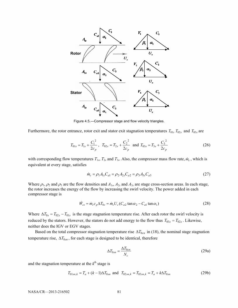
NASA/CR—2013-216502 81

Figure 4.5.—Compressor stage and flow velocity triangles.

Furthermore, the rotor entrance, rotor exit and stator exit stagnation temperatures sT01 sT02 and sT03 are

p

ss cCTT2

21

101 += , p

ss cCTT2

22

202 += and p

ss cCTT2

23

303 += (26)

with corresponding flow temperatures T1s, T2s and T3s. Also, the compressor mass flow rate, cm , which is equivalent at every stage, satisfies

333222111 asasasc CACACAm ρρρ === (27)

Where ρ1, ρ2 and ρ3 are the flow densities and A1s, A2s and A3s are stage cross-section areas. In each stage, the rotor increases the energy of the flow by increasing the swirl velocity. The power added in each compressor stage is

)tantan( 11220 αα aaccspccs CCUmTcmW −=∆=

(28)

Where sss TTT 01020 −=∆ is the stage stagnation temperature rise. After each rotor the swirl velocity is reduced by the stators. However, the stators do not add energy to the flow thus ss TT 0203 = . Likewise, neither does the IGV or EGV stages.

Based on the total compressor stagnation temperature rise cnT0∆ in (18), the nominal stage stagnation temperature rise, snT0∆ , for each stage is designed to be identical, therefore

c

cnsn N

TT 00

∆=∆ (29a)

and the stagnation temperature at the kth stage is

snaksn TkTT 0,01 )1( ∆−+= and snaksnksn TkTTT 0,03,02 ∆+== (29b)

Rotor

Stator

Rotor

Stator

NASA/CR—2013-216502 82

The compressor stage cross-sectional areas A1s, A2s and A3s are determined such that the axial flow velocities though each stage remain constant at the nominal operating condition. Thus, at nominal conditions we have

321 aaaan CCCC === . (31)

In this case, the nominal design axial flow speed is selected as Can = 150 m/s. Using (28)-(30), the nominal flow angles for the Nc identical stages are

IGVn αα =1 ,

+

∆= −

nancn

snn CU

T1

012 tantan αα , IGVnn ααα == 13 (32)

Where αIGV is the IGV exit angle which is used as the free design variable (within limits). Note, for identical stages, since the stator exit angle is the same as rotor entrance angle of the next stage, we have α3n = α1n. Also, using (25) together with (31), β1n, β2n and β3n can be determined. Here the range of allowable αIGV is determined by checking the so called de Haller number (Ref. 70). Next, using, (26), (27), (29) and (30), together with the ideal gas law expression for density and the adiabatic compression relations starting from the compressor inlet, the compressor cross-section areas at the kth stage are

1

1

,1

1,1

−

−=γ

γγ

ksnaan

acnks

TPC

RTmA

, 1

1

,2

1,2

−

−=γ

γγ

ksnaan

acnks

TPC

RTmA

and 1

1

,3

1,3

−

−=γ

γγ

ksnaan

acnks

TPC

RTmA

[k = 1 – Nc] (33)

Where R is the ideal gas constant. Finally, the compressor mean radius is

ht

htsm

AR

µµ

π −+

=11

41,1 (34)

Where µht = Rtip/Rhub is the hub-to-tip ratio at the inlet, which is a geometric design variable. Here the hub-to-tip ratio is selected as µht = 0.35. The resulting compressor stage hub and tip radii for this design are show in Figure 4.6, and the corresponding compressor stage angles are summarized in Table 4.2. Furthermore, the gas generator and power turbine angles as well as the rotational inertias computed based on the component mean radius values are also given in Table 4.2.

Figure 4.6.—Compressor hub and tip radius.

1 2 3 4 5 6 7 80

0.02

0.04

0.06

0.08

0.1

0.12

0.14

0.16

0.18

Stage Number

Radius, m

Tip Radius

Hub Radius

1 2 3 4 5 6 7 80

0.02

0.04

0.06

0.08

0.1

0.12

0.14

0.16

0.18

Stage Number

Radius, m

Tip Radius

Hub Radius

NASA/CR—2013-216502 83

TABLE 4.2.—COMPRESSOR AND TURBINE DESIGN PARAMETERS

Temperature rise or drop

Absolute angles

Relative angles

Mean radius

Rotational inertia

Compressor (8 Stage) ∆T0cn = 458.21°K

α1n = 40.0° α2n = 63.43° α3n = 40.0°

β1n = 53.79° β2n = 11.60° β3n = 53.79°

Rmc=0.12 m Jc=1.54 kg m2

Gas Generator Turbine (2 Stage) ∆T0ggtn = 458.21°K

α1n = 10.0° α2n = 58.38° α3n = 10.0°

β1n = 54.96° β2n = 20.49° β3n = 54.96°

Rmggt=0.13 m Jggt=0.26 kg m2

Power Turbine (2 Stage) ∆T0ptn = 412.22°K

α1n = 10.0° α2n = 53.38° α3n = 10.0°

β1n = 51.17° β2n = 24.23° β3n = 51.17°

Rmpt=0.24 m Jpt=0.98 kg m2

Figure 4.7.—Assumed flow angle deviations for off-nominal operation.

4.5 Analytical Calculation of Off-Nominal Characteristic Maps

Under transient conditions such as during gear ratio changes or during sudden main rotor power demands, the engine will undergo deviations about the nominal design operating point which is regulated by the engine fuel control. Therefore, it is necessary to model the off-nominal operation of compressor and turbine units. The off-nominal characteristics are typically described by compressor and turbine maps which show pressure ratio and isentropic efficiency as a function of mass flow for a given rotational speed as shown in (4). The compressor map can either be obtained experimentally or estimated analytically. In this investigation, compressor map data was not available, therefore a novel procedure is developed to analytically generate these maps for a given compressor design.

Since the stage areas and blade angles are fixed, the constant axial velocity condition (31) is only valid at the nominal operating point. For off-nominal operation, the axial velocity and the flow angles will deviate from nominal and vary from stage to stage. However, as discussed in (Ref. 70), since the flow exiting a rotor or stator is essentially attached to the blade, the exit flow deviation angles are negligible compared to the entrance flow deviation angles (See Figure 4.7).

cURotor

Stator

1β∆

n22 ββ =

2α∆

n23 αα =

1C

n1α1β

2C

2αn2β

3C

n3α3β

cU

cU

cU

cURotor

Stator

1β∆

n22 ββ =

2α∆

n23 αα =

1C

n1α1β

2C

2αn2β

3C

n3α3β

cU

cU

cU

NASA/CR—2013-216502 84

Based on this assumption, the kth stage flow angles in the cascade are

3,3

,22,2

1,3,1

nk

knk

kk

ααααα

αα

=

∆+=

= −

and

knk

nk

knk

,33,3

2,2

,11,1

βββββ

βββ

∆+=

=

∆+=

[k = 1 – Nc] (35a)

Where k,2α∆ k,1β∆ and k,3β∆ are the flow deviation angles during off-nominal operation. Also, since the initial entrance angle into the cascade is equal to the fixed exit angle of the IGV we have

IGVkk αααα === − 1,11,3,1 (35b)

Next, in order to compute the velocities and corresponding stagnation temperatures and pressures in a given stage, the stage entry conditions (which are equal to the exit conditions of the previous stage) are assumed to be known. In this way the results from stage k can be utilized in the computation of stage k+1 in the cascade. Starting with stage work and mass flow expressions in (27) and (28) and utilizing (24)-(26) together with the ideal gas law relations, we arrive at the following polynomial equation for the kth stage turbine exit axial velocity Ca2,k.

021

,211

,2 =++ −+ aCaC kakaγγ (36a)

With coefficients

γγ

β

βα

ksksks

cnp

nkspnckac

TAPRmca

TcUCUa

,01

1

,2,01

222

22,011,1

21

)cos(2

)cos()2tan2(−

=

+−−=

(36b)

for [k = 1 – Nc]. with

1,03,011,03,011,3,1 , , −−− === kskskskskaka PPTTCC (37)

Likewise utilizing the fact that Uc=0 in the stator section (or equivalently that ksks TT ,02,03 = ) we obtain the following polynomial equation for stator exit axial velocity Ca3,k.

021

,311

,3 =++ −+ bCbC kakaγγ (38a)

With coefficients

γ

γ

α

α

ksksks

cnp

nksp

TAPRmcb

Tcb

,02

1

,3,02

232

23,021

)cos(2

)cos(2−

=

−=

(38b)

for [k = 1 – Nc]. The cascade computation is initialized at the first stage, k=1, for a given ambient inlet condition Ta, and Pa, mass flow rate, cm , and rotation speed, Ωc. The subsequent stages are computed using the output of the previous stage as input for the next stage. Here the kth stage rotor exit stagnation pressure ksP ,02 is computed as

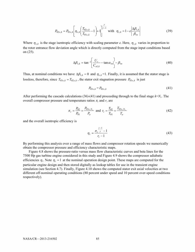
NASA/CR—2013-216502 85

1

,01

,02,,01,02 11

−

+

−=

γγ

ηks

ksksksks T

TPP with

n

kks

1

,1, 1

ββ

εη∆

−= (39)

Where ks,η is the stage isentropic efficiency with scaling parameter ε. Here, ks,η varies in proportion to the rotor entrance flow deviation angle which is directly computed from the stage input conditions based on (25).

nnka

ck C

U11

,1

1,1 tantan βαβ −

−=∆ − (40)

Thus, at nominal conditions we have 0,1 =∆ kβ and ks,η =1. Finally, it is assumed that the stator stage is lossless, therefore, since ksks TT ,02,03 = , the stator exit stagnation pressure ksP ,03 is just

ksP ,03 = ksP ,02 (41)

After performing the cascade calculations (36)-(41) and proceeding through to the final stage k=Nc. The overall compressor pressure and temperature ratios πc and rc are

a

Nsc P

PPP c,03

01

02 ==π and a

Nsc T

TTTr c,03

01

02 == (42)

and the overall isentropic efficiency is

1

11

−−

=

−

c

cc r

γγ

πη (43)

By performing this analysis over a range of mass flows and compressor rotation speeds we numerically obtain the compressor pressure and efficiency characteristic maps.

Figure 4.8 shows the pressure-ratio versus mass flow characteristic curves and beta lines for the 7500 Hp gas turbine engine considered in this study and Figure 4.9 shows the compressor adiabatic efficiencies ηc. Note 1=cη at the nominal operation design point. These maps are computed for the particular engine design and then stored digitally as lookup tables for use in the transient engine simulation (see Section 4.7). Finally, Figure 4.10 shows the computed stator exit axial velocities at two different off-nominal operating conditions (80 percent under speed and 10 percent over-speed conditions respectively).

NASA/CR—2013-216502 86

Figure 4.8.—Compressor pressure ratio versus

air mass flow.

Figure 4.9.—Compressor adiabatic efficiency

versus mass flow.

Figure 4.10.—Stator exit axial velocities at two different off-

nominal operating conditions; (a) ] 6.0 , 8.0[ cnccnc mm =Ω=Ω ; (b) ] 05.1 , 10.1[ cnccnc mm =Ω=Ω .

50

4 6 8 10 12 14 16 18

10

20

30

40

Compressor mass flow rate, cm (kg/s)

cπ

cnc ΩΩ /1.0 1.05

1.1

0.950.90.85

12.0=cβ*Surge

line

14.0=cβ

16.0=cβ

18.0=cβ2.0=cβ

24.0=cβ 22.0=cβ50

4 6 8 10 12 14 16 18

10

20

30

40

Compressor mass flow rate, cm (kg/s)

cπ

cnc ΩΩ /1.0 1.05

1.1

0.950.90.85

12.0=cβ*Surge

line

14.0=cβ

16.0=cβ

18.0=cβ2.0=cβ

24.0=cβ 22.0=cβ

4 6 8 10 12 14 16 180.75

0.8

0.85

0.9

0.95

1

Compressor mass flow rate, cm (kg/s)

cη

cnc ΩΩ /1.0 1.05

1.10.95

0.9

0.85 1.150.8

0.750.7

4 6 8 10 12 14 16 180.75

0.8

0.85

0.9

0.95

1

Compressor mass flow rate, cm (kg/s)

cη

cnc ΩΩ /1.0 1.05

1.10.95

0.9

0.85 1.150.8

0.750.7

4 6 8 10 12 14 16 180.75

0.8

0.85

0.9

0.95

1

Compressor mass flow rate, cm (kg/s)

cη

cnc ΩΩ /1.0 1.05

1.10.95

0.9

0.85 1.150.8

0.750.7

1 2 3 4 5 6 7 80

50

100

150

1 2 3 4 5 6 7 80

50

100

150

Can = 150 m/s

Can = 150 m/s(b)

(a)

Compressor Stage

Stator Exit Axial Velocity,

m/s

1 2 3 4 5 6 7 80

50

100

150

1 2 3 4 5 6 7 80

50

100

150

Can = 150 m/s

Can = 150 m/s(b)

(a)

Compressor Stage

Stator Exit Axial Velocity,

m/s

NASA/CR—2013-216502 87

4.6 Engine Closed-Loop Fuel Control

To maintain the engine output shaft set-point speed during operation, a closed-loop fuel controller is required to regulate the fuel flow into the combustion chamber. A schematic of this arraignment is depicted in Figure 4.11. Here a Proportional Integral Derivative (PID) control law

ptdptIptpf ekdtekekmfff ++= ∫ with ptptpt set

e Ω−Ω= (44)

is utilized for this purpose with instantaneous fuel flow into the combustion chamber fm . Where the PID control, with gains fpk , fIk and fdk , determines the fuel flow rate in order to regulate the power turbine set-point speed error ept to zero. It is also necessary to account for the maximum and minimum fuel flow rate constraints minfm and maxfm as well as compressor maximum speed limit maxcΩ which is accomplished through the use of two saturation blocks. Finally, to prevent windup of the PID integrator block, the back-calculating gains fbk and Ωbk on the fuel saturation and compressor speed saturation blocks are utilized. The block diagram of the complete engine fuel control system is shown in Figure 4.12.

The stability and performance characteristics of the closed-loop engine system are strongly affected by the gain values fpk , fdk and fIk . The value of these gains were selected by trial-and-error until a stable engine response was achieved. The engine fuel control system parameters are given in Table 4.3.

Figure 4.11.—Engine with closed-loop PID fuel control

fmptΩ

esetptΩ

Gas Generator

Power Turbine

ggtΩ

Load

cm

TaPa

-

FuelControl

Law

cΩ

fmptΩ

esetptΩ

Gas Generator

Power Turbine

ggtΩ

Load

cm

TaPa

-

FuelControl

Law

cΩ

NASA/CR—2013-216502 88

Figure 4.12.—Engine fuel control block diagram.

TABLE 4.3.—ENGINE FUEL CONTROL SYSTEM PARAMETERS Parameter Value Proportional fuel control gain,

fpk ......................................4.0×10-3 kg

Integral fuel control gain, fIk ...................................... 5.0×10-3 kg/sec

Derivative fuel control gain, fdk .................................. 4.0×10-4 kg-sec

Compressor speed back-calculating gain, Ωbk .................. 0.018 kg/sec Fuel rate back-calculating gain,

fbk .......................................... 100/sec Minimum fuel rate, minfm .................................................. 0.03 kg/sec Maximum fuel rate, maxfm ................................................ 0.337 kg/sec Compressor speed limit, maxcΩ ......................................... 27,500 RPM

4.7 Transient Gas Turbine Engine Simulation

The dynamic simulation model of the gas turbine consists of a mixed set of ordinary differential and nonlinear algebraic equations. During each simulation time step, the mass flow through each component (compressor, gas generator turbine and power turbine) is interpolated using the numerically generated characteristic maps for the instantaneous rotation speed and upstream and downstream pressure states. As was shown in (Ref. 80) a non-iterative solution to the equations can be obtained through forward substitution provided that the equations are solved in the proper sequence. Here equations are arranged in order to explicitly generate the output values by forward substitution. At each time step, the differential equations are integrated by means of an explicit scheme, thus obtaining the new values of the system plenum pressures, fuel control input and shaft rotational speeds. As was shown in (Ref. 80) when the equations are ordered in accordance with the stream direction of the gas turbine model this results in the

PIDPID

NASA/CR—2013-216502 89

proper solution order. Figure 4.13 to Figure 4.20 summarize the non-iterative transient gas turbine engine simulation model which is implemented in the Matlab Simulink environment. Finally, Figure 4.21 and Figure 4.22 show the gas turbine engine response to a simulated shock load event. In this loading scenario (Figure 4.21(a)) the main rotor drag is suddenly dropped by 50 percent at time t=5.0 sec and then suddenly increased t=15.0 sec. This scenario could result due to a sudden drop (or increase) in main rotor collective pitch. Similar shock load events can also occurs during upshift and downshift events (see Sections 5.0 and 6.0). This simulation shows that the closed-loop fuel control gains indeed render the system stable. The simulation also verifies correct functioning of the forward substitution method since the mass flows through each component converge to identical at steady state values.

Figure 4.13.—Gas turbine engine with fuel control and rotor load—main simulation block.

NASA/CR—2013-216502 90

Figu

re 4

.14.

—Tw

o-sp

ool g

as tu

rbin

e en

gine

sim

ulat

ion

bloc

k

NASA/CR—2013-216502 91

Figure 4.15.—Compressor simulation block.

Figure 4.16.—Inter compressor/combustion chamber plenum.

NASA/CR—2013-216502 92

Figure 4.17.—Combustion chamber simulation block.

Figure 4.18.—Gas generator turbine simulation block.

NASA/CR—2013-216502 93

Figure 4.19.—Inter turbine plenum.

Figure 4.20.—Power turbine simulation block.

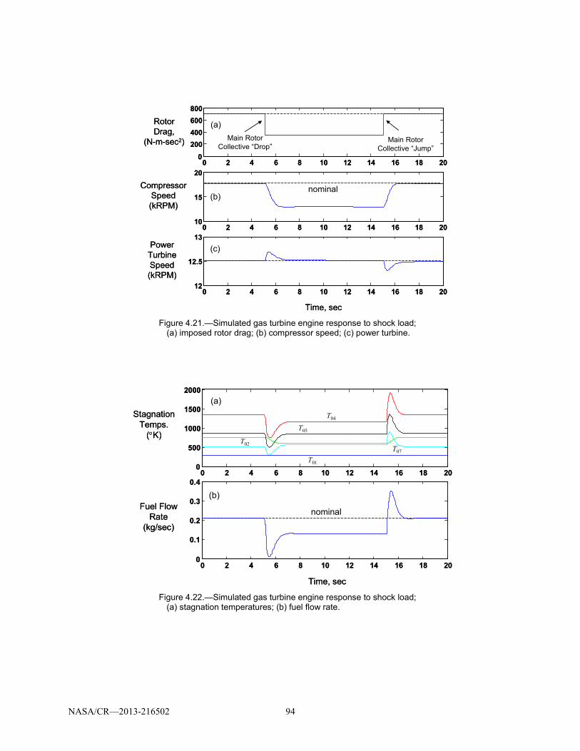
NASA/CR—2013-216502 94

Figure 4.21.—Simulated gas turbine engine response to shock load;

(a) imposed rotor drag; (b) compressor speed; (c) power turbine.

Figure 4.22.—Simulated gas turbine engine response to shock load;

(a) stagnation temperatures; (b) fuel flow rate.

Rotor Drag,

(N-m-sec2)

Compressor Speed (kRPM)

Power Turbine Speed (kRPM)

0 2 4 6 8 10 12 14 16 18 200

200400600800

0 2 4 6 8 10 12 14 16 18 2010

15

20

0 2 4 6 8 10 12 14 16 18 2012

12.5

13

Time, sec

(a)

(b)

(c)

Main Rotor Collective “Drop”

Main Rotor Collective “Jump”

nominal

Rotor Drag,

(N-m-sec2)

Compressor Speed (kRPM)

Power Turbine Speed (kRPM)

0 2 4 6 8 10 12 14 16 18 200

200400600800

0 2 4 6 8 10 12 14 16 18 2010

15

20

0 2 4 6 8 10 12 14 16 18 2012

12.5

13

Time, sec

(a)

(b)

(c)

Main Rotor Collective “Drop”

Main Rotor Collective “Jump”

nominal

0 2 4 6 8 10 12 14 16 18 200

500

1000

1500

2000

Stagnation Temps.

(°K)

T04

T05

T02T07

T01

0 2 4 6 8 10 12 14 16 18 200

0.1

0.2

0.3

0.4

Time, sec

Fuel Flow Rate

(kg/sec)

nominal

(a)

(b)

0 2 4 6 8 10 12 14 16 18 200

500

1000

1500

2000

Stagnation Temps.

(°K)

T04

T05

T02T07

T01

0 2 4 6 8 10 12 14 16 18 200

0.1

0.2

0.3

0.4

Time, sec

Fuel Flow Rate

(kg/sec)

nominal

(a)

(b)

NASA/CR—2013-216502 95

5.0 Gearbox Dynamics Modeling 5.1 Introduction

It is well known that gear tooth meshing stiffness fluctuations and tooth backlash effects are a significant source of vibration and instability in geared rotor systems. The overall objectives of this portion of the project can be summarized as follows;

• Develop gear system dynamics models to predict torsional vibration levels during variable speed

operation • Conduct experimental evaluation of gear dynamics model under variable speed conditions • Develop computationally efficient tools to asses gear vibration levels during variable speed

operation • Explore gearbox/shaft dynamic interactions and stability behavior via variable speed dynamic

simulations

The topic of gear induced vibration and its mitigation has been widely studied and remains an important topic in propulsion system research and design. For meshing gear pairs, the number of teeth in contact is kinematically a function of the gear rotation angle. Since gear mesh stiffness due to elastic tooth bending is related to the instantaneous number of teeth in contact, this results in time-varying stiffness fluctuations which can excite vibrations and induce parametric instability (Refs. 84 to 95). For a spur gear pair, References 84 to 87 experimentally demonstrated that gear mesh stiffness parametric effects excited large amplitude period-1 (1T) and period-n (nT) subharmonic responses. For gear mesh harmonics in the vicinity of natural frequency multiples, these vibrations resulted tooth loss-of-contact which produced nonlinear chattering and jump phenomena (Refs. 85 and 86). Several reduced-order lumped-parameter spur gear dynamic models including time-varying mesh stiffness and clearance nonlinearities were analyzed by References 85, 86 and 88. Furthermore, References 89 and 90 explored the effects of mesh stiffness variation on two-stage gear-trains and planetary gear transmissions. Here the undamped equations-of-motion with an idealized square wave type mesh stiffness was considered and conditions for primary, secondary and combination parametric instabilities were derived via perturbation analysis. Additionally, the roles of mesh damping, involute contact ratio, and tooth sliding friction on spur gear dynamics have been explored (Refs. 91 to 95).

Another body of gear vibration research has focused full scale system modeling of coupled gear/rotor/bearing vibrations (Refs. 96 to 101). However, in most of these studies gear backlash and mesh stiffness variations were not considered since the scope was primarily on modal analysis and coupling between transverse and torsional motions (Refs. 97 and 98), and torsion, lateral and axial motions (Refs. 99, 100, and 12) in large degree-of-freedom gear/rotor/bearing systems. These studies typically considered a constant (nominal) value of gear tooth mesh stiffness together with shaft and bearing compliance. The results offered valuable insights into the effects of gear, shaft and bearing placement on modal coupling and natural frequencies. However, the influence of the coupled substructure interactions on gear-mesh induced parametric instabilities was not determined. Finally, Reference 101 considered a periodically stepped alloy shaft for reducing torsional gear vibrations via wave propagation stop-bands. Here however, the focus was on blocking transmitted vibrations and not on suppressing the gear tooth mesh instabilities.

Despite this large body of gear dynamics research, the majority of the work has focused on constant speed operation where the system is linear periodically time-varying. The exceptions to this are investigations into nonlinear backlash effects (Refs. 85 to 88). However, these studies focused on quasi-steady response under slow-speed RPM changes and did not characterize transient gear vibrations nor the effects of spinup or spindown acceleration rates. The following sections will address these issues as well as the four main objectives stated at the beginning of this section.

NASA/CR—2013-216502 96

Figure 5.1.—Spur gear/shaft system dynamic model.

5.2 Spur Gear/Shaft Structural Dynamics Model

To analyze the gear system dynamics, a structural dynamic model of the spur gear/shaft system depicted in Figure 5.1 is developed. Here, a torsionally flexible input shaft, length Ls, drives a load inertia, JL, and a resistive load torque, TL, through as single spur gear pair. In this model, the shaft elastic twist

),(ˆ txsφ is defined over the domain ]0[ sLx << . On the input side (at x = 0). The shaft is rigidly fixed to the input coupling thus has boundary

condition

0),0(ˆ =tsφ (1)

Furthermore during operation, it is assumed that the input shaft rotation, φ0, is driven with angular velocity Ω

tΩ=0φ (2)

Based on this, the total rotations φg1(t) and φg2(t) of gears 1 and 2 are

),(ˆ)(1 tLtt ssg φφ +Ω= and )(ˆ)( 2122 ttnt gg φφ +Ω−= (3)

where gear 1 is fixed to the shaft at x = Ls and )(ˆ2 tgφ is the elastic twist deviation (due to tooth mesh

compliance) from the nominal rigid-body rotation dictated by the gear ratio n12

2

112 Z

Zn = (4)

where Z1 and Z2 are number of teeth on gear 1 and 2 respectively.

5.2.1 Lumped Spur Gear Model Here the gears are modeled as lumped rigid disks with base radius, Rbi, mass, mgi, and rotational

inertia, Jgi, [for i = 1, 2]. The tooth mesh compliance is accounted for by a spring stiffness element, km(t), acting along the line-of-action (at pressure angle αPA). See Figure 5.2.

JL

TL

Ls

φ0 = Ωtφg1(t)

φg2 (t)

x),(ˆ txsφ

Input Shaft

Spur Gear Pair

LoadZ2, Jg2, mg2

Z1, Jg1, mg1

JL

TL

Ls

φ0 = Ωtφg1(t)

φg2 (t)

x),(ˆ txsφ

Input Shaft

Spur Gear Pair

LoadZ2, Jg2, mg2

Z1, Jg1, mg1

NASA/CR—2013-216502 97

Figure 5.2.—Lumped gear-pair model, inertias and tooth mesh stiffness.

For gears with non-integer contact ratio, cr, the number of teeth in mesh fluctuates between the

integers ceil(cr) and floor(cr) as a function of gear rotation.

PAppbpbp RRcp

RaRRaRcr αtan)(1)( )( 212

22

22

12

1 +−−++−+= (5)

Where cp is gear circular pitch, Rpi [i = 1, 2] is pitch radius

π2 cpZR i

pi= and PApibi RR αcos= [ i = 1,2] (6)

and tooth addendum

πcpa = (7)

Since km(t) is proportional to the number of teeth in contact at any instant, at constant rotation speed, km(t) switches between maximum and minimum stiffness values kmax and kmin with square wave-like variation which has Fourier series representation

∑=

Ω+Ω+=hN

ncnsnm tnZktnZkktk

1110 )]cos()sin([)( (8-a)

with

maxmin0 )1()2( kcrkcrk −+−= (8-b)

and

ππn

ncrkkksn])2(2[ cos1)( minmax

−−−= and

ππ

nncrkkkcn

])2(2[ sin)( minmax−

−= (8-c)

Where Nh is the number of expansion harmonics and Z1Ω is the gear mesh frequency (and associated fundamental period Tp = 2π/Z1Ω). Similar to Reference 102, the gear mesh stiffness is estimated by considering each tooth as a tip loaded cantilever beam with average tooth dimensions in series with gear body stiffness values kb1 and kb2. For [1 < cr < 2]

NASA/CR—2013-216502 98

21

min 1211

btb kkk

k++

= and

21

max 1111

btb kkk

k++

= (9)

and tooth stiffness, kt, and gear body stiffness kbi

3

3

)(cos32

badcpEk

PAt +=

α and 22

24

hibi

hibi

RRdRGk

−=

π [i = 1,2] (10)

with gear elastic and shear moduli, E and G, tooth dedendum, b=1.25*a, face width d, and hub radius Rhi [i = 1, 2].

5.2.2 Work and Energy Expressions Based on the above lumped gear model approximation, the gear/shaft system kinetic energy, T, can be

expressed as

)]()()([21]),(ˆ[

21 2

222110

2 tJJtJdxtxJT gLgggL

ssss

φφφρ

+++Ω+= ∫ (11a)

where “• “ indicates differentiation with respect to time, t, Also, ρs is the shaft material density and Js is the shaft polar moment of area defined in terms of shaft inner and outer radii, Rsi and Rso,

)(2

44sisos RRJ −=

π (11b)

Furthermore, the total system strain energy, U, due to both shaft torsional elasticity and gear tooth mesh compliance is

22211

0

2 )]()()[(21),(ˆ

21 tRtRtkdxtxJGU gbgbm

L

sss

s

φφφ ++′= ∫ (12)

where “ ' “ indicates differentiation with respect to the shaft axial coordinate x, and Gs is the shaft material shear modulus. Note, in the second term of the above strain energy expression, the quantity

)()()( 2211 tRtRtu gbgbm φφ += (13)

is the gear tooth mesh deflection um(t) along the line-of-action. In addition, dissipation effects are accounted for via the Rayleigh dissipation function

222110

2 )]()()[(21 ),(ˆ

21 tRtRtkdxtxJGD gbgbmm

Lssss

sφφξφξ

++′= ∫ (14)

where ξs and ξm are shaft and gear mesh proportional viscous damping parameters. Finally, the virtual work due to the driven load torque TL and prescribed angular acceleration rate Ω is

)(ˆ))(( 2212 tJJnTW ggLL φδδ Ω++−= (15)

NASA/CR—2013-216502 99

Figure 5.3.—Two-DOF shaft torsional finite element.

5.2.3 Gear/Shaft Finite Element Model In order analyze the coupled gear/shaft system structural dynamics, a finite element model (FEM) of

the gear/shaft system in Figure 5.1 is developed. The shaft is discretized into nel, uniform torsional elements each with length Lel=Ls/nel. Each element, as shown in Figure 5.3, has two nodes with 1 torsional degree of freedom (DOF) per node. The jth element DOF vector is

=

+ )(ˆ)(ˆ

)(1

, tt

tqj

jjel φ

φ (16)

where )(ˆ tjφ is the shaft elastic twist DOF at the jth nodal location.

Using the standard linear interpolation element, the shaft twist, ),(ˆ, txjsφ , within jth element domain

[ ]elLx ≤≤0 is

)()(),(ˆ,, tqxNtx jeleljs =φ (17a)

with corresponding elemental shape function vector

[ ]elelel LxLxxN //1)( −= (17b)

After fusing the adjacent shaft nodes and applying the constraints (1) and (3), the global DOF vector of the discretized gear/shaft system becomes

=

)(ˆ)(

)(2 t

tqtq

g

s

φ (18a)

Which is composed of shaft twist DOF vector with Nn nodes

TNssss ttttq

n])(ˆ)(ˆ)(ˆ[)( ,2,1, φφφ = (18b)

and the output gear elastic rotation )(ˆ2 tgφ .

y

x

z

Lel

node j+1

node j

)(ˆ tjφ

)(ˆ1 tj+φ

Rsi

Rso

y

x

z

Lel

node j+1

node j

)(ˆ tjφ

)(ˆ1 tj+φ

Rsi

Rso

NASA/CR—2013-216502 100

Next, utilizing the system work, energy and dissipation expressions in (11), (12), (14) and (15) together with the FEM discretization (17), the overall gear/shaft system equations-of-motion are synthesized via Lagrange’s Equations

F=∂∂

+∂∂

+∂∂

−

∂∂

qD

qU

qT

qT

dtd

(19)

The resulting linear time-varying equations-of-motion are

)()()()()()( ttqttqttq FKCM =++ (20a)

With system inertia matrix

++

=Lg

gggs

JJNNJM T

2

111

00

M (20b)

damping matrix

+= 2

2121

1211121

)()()()(

)(bmmgbbmm

gbbmmggbmmss

RtkNRRtkNRRtkNNRtkK

t T

TT

ξξξξξ

C (20c)

stiffness matrix

+= 2

2121

1211121

)()()()(

)(bmgbbm

gbbmggbms

RtkNRRtkNRRtkNNRtkK

t T

TT

K (20d)

and generalized force vector F obtained from qW Tδδ F=

Ω++Ω−

=

)( 212

11

gLL

Tgg

JJnTNJ

F (20e)

Here, the DOF selection matrix, 1gN , defined in (21), extracts the gear 1 twist DOF (i.e., shaft twist at x = Ls) from the shaft twist DOF vector qs

)()(]1000[),(ˆ1 tqNtqtL sgsss ≡= φ (21)

Also, the mass, stiffness and damping submatrices, Ms, Ks and Cs in (20) are formed according to the FEM approach from the elemental mass stiffness and damping matrices given as

∫=elL

elTelssels dxxNxNJM

0, )()(ρ and dxxNxNJGK

sLel

Telssels )()(

0, ∫ ′′= (22a)

and

dxxNxNJGCsL

elT

elsssels )()(0, ∫ ′′= ξ (22b)

NASA/CR—2013-216502 101

Figure 5.4.—Gear backlash; (a) gear pair with tooth clearance (b) gap function.

5.2.4 Gear-Tooth Clearance and Backlash Effects Next the model is modified to include nonlinear backlash effects due to tooth gap clearance hgap.

Specifically similar to References 85 to 88, the so called gap function is introduced (see Figure 5.4). Based on this, the gear/shaft system equations-of-motion including nonlinear backlash become

FKCM =

++

)](ˆ[)(

)()()()(2 tgtq

ttqttqg

s

φ (23a)

with gap function

−<+

≤

>−

=

22

22

22

22

22

2

2ˆ

2ˆ

2 |ˆ|0

2ˆ

2ˆ

)](ˆ[

b

gapg

b

gapg

b

gapg

b

gapg

b

gapg

g

Rh

Rh

RhR

hR

h

tg

φφ

φ

φφ

φ (23b)

Where the system mass, stiffness and damping matrices and generalized force vector are identical to those defined in (20).

5.3 Single Gearbox/Shaft System Variable RPM Response

To explore the variable speed response of gearbox/shaft system presented in the previous section, the parameters for a representative rotorcraft driveshaft subsystem are utilized for analysis. These parameters are summarized in Table 5.1.

Figure 5.5 shows the [Ω = 0 to 3000 to 0] RPM spinup-spindown vibration response of the gear mesh deflection (13) for three load torque levels.

Here the variable tooth stiffness results in vibratory behavior under constant load torque conditions due to parametric excitations. The dotted lines at ±10µm in Figure 5.5 indicate the backlash limits

]2/2/[ gapgap huh ≤≤− also shown Figure 5.4(b). Tooth deflection greater than 2/gaph indicates front side tooth contact and tooth deflection less than 2/gaph− means back-side contact. Deflections within

]2/2/[ gapgap huh ≤≤− indicate loss-of-contact. Figure 5.5(a) shows that for lower torque values the tooth remains in single-sided contact (deflection remains near upper limit). As the load torque is increased, Figure 5.5(c) shows that the tooth begins to chatter back and forth between the upper and lower limits (double sided contact). This double sided contact occurs for certain rotational speeds only. The magnitude

NASA/CR—2013-216502 102

of the chattering is proportional to the load torque level. It is also noted that the spinup and spindown vibration amplitudes are not the same. This difference is again a result of the nonlinear dynamics nature of the system.

Utilizing the above nonlinear dynamic model for the gear/shaft system, the variable speed dynamic behavior is further investigated in Section 5.4. To assess the validity and performance of this model, the analytical transient vibration response predictions will be compared with measurements from a variables speed gearbox/shaft test rig experiment.

TABLE 5.1.—GEARBOX-SHAFT SYSTEM PARAMETERS Parameter Value Number of teeth, Zi ................................................ Z1=42, Z2 =30 Pressure angle, αPA .................................................................. 25° Circular pitch, cp ......................................................... 0.0157 m-1 Contact ratio, cr ................................................................. 1.4954 Face width, d ..................................................................... 18 mm Gear Inertia, Ji ..................................... J1=0.243, J2 =0.063 kg-m2 Load Inertia, JL .........................................................JL=2.0 kg-m2 Load Torque, TL ............................................................. Various* Backlash gap clearance, h .................................................. 20 µm Shaft Length, L ...................................................................... 6 m Density (shaft) ............................................................ 2800 kg/m3 Elastic modulus (gear), E ................................................ 200 GPa Shear modulus (shaft), G .................................................. 27 GPa Cross-section polar area moment, Js ...................... 4.469×10-6 m4

*Various values used in the investigation

Figure 5.5.—Gear mesh vibration response for 0-3000-0 RPM ramp input;

(a) TL = 100 Nm; (b) TL = 200 Nm; (c) TL = 300 Nm.

20 µm gap

20 µm gap

20 µm gap

Tooth Deflection,

µm

Time, secSpinup

(+100 RPM/Sec)[Ω = 0 to 3000 RPM]

(a)

(b)

(c)

Spindown(-100 RPM/Sec)

[Ω = 3000 to 0 RPM]

20 µm gap

20 µm gap

20 µm gap

Tooth Deflection,

µm

Time, secSpinup

(+100 RPM/Sec)[Ω = 0 to 3000 RPM]

(a)

(b)

(c)

Spindown(-100 RPM/Sec)

[Ω = 3000 to 0 RPM]

NASA/CR—2013-216502 103

5.4 Variable Speed Gear/Shaft Model Experimental Validation

To account for effects of gear meshing on the system behavior, a nonlinear time varying dynamic model including the effects of gear tooth flexibility, non-unity contact ratios, backlash clearance, gear inertias and load torque has been developed (see Section 5.2). To validate this model, an experimental gear dynamics test rig at the University of Tennessee has been utilized, see Figure 5.6.

The test rig consists of a DC electric motor with PID speed controller which drives a single-stage spur gearbox (also capable of multistage). The input shaft is fitted with an inductively coupled torque and RPM sensor and an optical encoder. The gearbox output drives a magnetic brake which has a manual brake torque setting. Table 5.2 and Figure 5.7 summarize the experimental test setup.

Figure 5.6.—Spur gear dynamics test rig (Univ. Tenn.).

Figure 5.7.—Spur gear dynamics test rig experimental setup

TABLE 5.2.—GEARBOX DYNAMICS TESTRIG PARAMETERS

Gears Input shaft Gear type Spur Material ................................................... Steel

Length .................................................... 18 in. Diameter (solid) .................................... 5/8 in.

Number of teeth (input) ............................... Z1=30 Number of teeth (output) ............................. Z2=42 Tooth module ............................................... 5 mm Diametral pitch................................................ 200 Pressure angle ................................................. 25° Addendum .................................................... 5 mm Dedendum ............................................... 6.25 mm Face width .................................................. 25 mm Gap clearance (nominal) ............................. 50 μm

Motor speed controller P-gain, kp .............................................. 1×10–4 I-gain, ki ............................................... 1×10–6 D-gain, kd .................................................... 20

Load Rotational inertia, JL .................. 0.0632 kg m2 Brake settings, TL .............. 10, 20 and 30 in-lb

DC Motor Torque Sensor

Spur Gear Pair

Magnetic BrakeEncoder

ETAC AA Filter Cutoff Freq10k Hz

DAQ Sampling Freq20 kHz

PC

PID Speed

Control

Ramp

dSpace1103

Torque Setting (Manual Adjust)

Z1=30(input)

Z2=42(output)

DC Motor Torque Sensor

Spur Gear Pair

Magnetic BrakeEncoder

ETAC AA Filter Cutoff Freq10k Hz

DAQ Sampling Freq20 kHz

PC

PID Speed

Control

Ramp

dSpace1103

Torque Setting (Manual Adjust)

DC Motor Torque Sensor

Spur Gear Pair

Magnetic BrakeEncoder

ETAC AA Filter Cutoff Freq10k Hz

DAQ Sampling Freq20 kHz

PC

PID Speed

Control

Ramp

dSpace1103

Torque Setting (Manual Adjust)

Z1=30(input)

Z2=42(output)

NASA/CR—2013-216502 104

Finally, the gear pair contact ratio of this spur gear pair is calculated to be cr = 1.495. To perform the experimental validation, several variable RPM tests under three different brake

settings (load torque, TL = 10, 20 and 30 in-lb) were performed to validate the high frequency gear mesh dynamics model. In each test the motor set-point RPM was ramped linearly from [0 - 3000 - 0] RPM over 60 sec while the input shaft speed and torque data were collected. Figure 5.8 shows the ramped RPM profile and Figure 5.9 to Figure 5.11 show the resulting input shaft load torque. Here Figure 5.9 to Figure 5.11(a) give the experimentally measured load torque while Figure 5.9 to Figure 5.11(b) show the corresponding predicted values from the model.

Figure 5.8.—Motor speed versus time, 0-3000-0 RPM ramp test 1.

Figure 5.9.—Input shaft torque versus time during 0-3000-0 RPM

ramp test 1, TL= 10 in-lb, (a) UT gearbox test rig (Exp), (b) gearbox dynamics model (SIM).

0 10 20 30 40 50 600

500

1000

1500

2000

2500

3000

3500

time, sec

Mot

or, R

PM

0 10 20 30 40 50 600

500

1000

1500

2000

2500

3000

3500

time, sec

Mot

or, R

PM

0 10 20 30 40 50 605

10

15

20

torq

ue, i

n-lb

, (EX

P)

0 10 20 30 40 50 605

10

15

20

torq

ue, i

n-lb

, (SI

M)

time, sec

(a)

(b)

0 10 20 30 40 50 605

10

15

20

torq

ue, i

n-lb

, (EX

P)

0 10 20 30 40 50 605

10

15

20

torq

ue, i

n-lb

, (SI

M)

time, sec

(a)

(b)

NASA/CR—2013-216502 105

Figure 5.10.—Input shaft torque versus time during 0-3000-0 RPM

ramp test 2; TL= 20 in-lb, (a) UT gearbox test rig (Exp), (b) gearbox dynamics model (SIM).

Figure 5.11.—Input shaft torque versus time during 0-3000-0 RPM

ramp test 3; TL= 30 in-lb, (a) UT gearbox test rig (Exp), (b) gearbox dynamics model (SIM).

In each test, the torques predicted by the model agree with the measured dynamic torque behavior for

the variable RPM condition. During both spinup and spindown, the model predicts jumps in dynamic torque amplitude. The main discrepancies occur just after the transition from spin-up to spin-down (near t = 30 sec). Here the measured transient torque spikes are larger than the model predictions. This could be attributed to some nonmodeled system looseness or backlash in the gear-shaft spline connections. However, as seen in Figure 5.9 to Figure 5.11, the dynamic torque amplitude predicted by the model are comfortably within 25 percent of the measured values during the constant spinup (0 < t < 30 sec) and spindown portions (30 < t < 60 sec). Furthermore, the jumps occur nearly at the same RPM values. This jump phenomena is due to both linear and nonlinear effects. As the mesh harmonics nZ1Ω1 pass through the system natural frequencies resonances are excited however nonlinear behavior due to gear backlash

0 10 20 30 40 50 6020

25

30

35

torq

ue, i

n-lb

, (EX

P)

0 10 20 30 40 50 6020

25

30

35to

rque

, in-

lb, (

SIM

)

time, sec

(a)

(b)

0 10 20 30 40 50 6020

25

30

35

torq

ue, i

n-lb

, (EX

P)

0 10 20 30 40 50 6020

25

30

35to

rque

, in-

lb, (

SIM

)

time, sec

(a)

(b)

0 10 20 30 40 50 6035

40

45

50

torq

ue, i

n-lb

, (EX

P)

0 10 20 30 40 50 6035

40

45

50

torq

ue, i

n-lb

, (SI

M)

time, sec

(a)

(b)

0 10 20 30 40 50 6035

40

45

50

torq

ue, i

n-lb

, (EX

P)

0 10 20 30 40 50 6035

40

45

50

torq

ue, i

n-lb

, (SI

M)

time, sec

(a)

(b)

NASA/CR—2013-216502 106

and tooth clearance are also a critical feature of the model and necessary to accurately predict the measured values.

5.5 Dual Gearbox/Shaft System Interactions Under Variable RPM

In this section the nonlinear dynamic interactions between two gearboxes coupled by a long torsionally flexible shaft. Such configurations are common in rotorcraft propulsion systems including tailrotor and cross-shafting drivelines. The shaft flexibility induces dynamic phasing between the two upstream and downstream gearboxes. This dynamic phasing together with the kinematic dependence of the gear tooth mesh stiffness on the gear rotation induces a nonlinear dynamic interaction not explored in previous single-stage or rigid-shaft gear system investigations.

For constant speed operation, Reference 90 showed that gear mesh stiffness variations in a single stage gear system can be effectively modeled as a square wave with frequency NtΩ where Nt is the number of teeth in mesh and Ω is the rotation speed. In the case of multistage gear systems, the critical importance of relative gear mesh phasing was demonstrated in Reference 13. Here, the concept of static mesh phasing, where individual gear mesh pairs are phased to cancel out or suppress the vibration from previous stages, was explored in the design of a multistage planetary gear system. For constant speed operation, the “built in” or static design mesh phasing was effective at reducing mesh stiffness induced gear system torsion vibrations.

It is clear from the existing research that the relative mesh phasing between different gear sets in a multistage gear train is a key design parameter which has a significant impact on the system vibration and stability characteristics for constant speed operation. However, the case of variable speed operation has not been explored. Furthermore, previous investigations have only considered the case of constant mesh phase between two gear sets, however in certain situations (such as when long cross-shafting and large dynamic windup is involved) this assumption may not be adequate. This paper explores nonlinear time-varying torsional dynamic behavior of a gear driven system involving two gearboxes coupled by a torsionally elastic shaft. See Figure 5.12.

Such configurations are common in many rotorcraft propulsion systems including tailrotor and cross-shafting drivelines. In this situation, if the flexible shaft connecting the two gear-sets has a nonnegligible windup, the relative phase becomes a dynamic variable related to the shaft twist resulting in a nonlinear time-varying gear mesh stiffness. Nonlinear dynamic phase interactions of this nature between gear sets has not been investigated in the literature, hence the aim of this study is to explore this effect.

Figure 5.12.—Dual gearbox-elastic shaft system.

NASA/CR—2013-216502 107

5.5.1 Dual Gearbox/Shaft System Model To facilitate analysis, the equations-of-motion of a dual stage, spur gear/shaft system including gear

mesh stiffness variations and shaft torsional dynamics is derived. See Figure 5.12. Here, gears in mesh pair a-b are modeled as rigid disks, with rotations φa and φb, rotational inertia Ja and Jb, and number of teeth Za and Zb. Gear tooth meshing is accounted for by spring stiffness, abmk , acting along the line-of-action in series with backlash gap clearance h.

Due to the periodic nature of the mesh stiffness with respect to gear rotation, the gear mesh stiffness functions, )( 112

φmk , )( 334φmk for the upstream and downstream gearboxes I and II (see Figure 5.12) can

be expressed in a Fourier series as

∑

∑

=

=

++=

+=

h

h

N

nIIIppm

N

nppm

nZn

crnkcrkk

nZn

crnkcrkk

1,333

1111

)cos() sin(2)(

)cos() sin(2)(

34

12

γφππφ

φππφ

(24)

Where γI,II is the relative mesh phase angle between gearboxes I and II (which is a free design parameter) and Nh is the number of expansion harmonics. By considering the intermediate shaft elastic twist, ),(ˆ txsφ , the elastic gear mesh deflections, u12(t) and u34(t), and gear ratios n12 and n34

2

1

2

112 Z

ZRRn

b

b =≡ and 4

3

4

334 Z

ZRRn

b

b =≡ (25)

the total gear rotations, )(tiφ [i=1-4], of the dual gearbox-shaft system in Figure 5.12 are

tt Ω=)(1φ , tntuR

tb

Ω−= 12122

2 )(1)(φ (26a)

),(ˆ)(1)( 12122

3 tLtntuR

t sb

φφ +Ω−= ,

−Ω+−+= ),(ˆ)()()( 12

2

1234

4

344 tLtn

Rtun

Rtut s

bbφφ (26b)

with shaft elastic constraint

0),0(ˆ =tsφ (26c)

Here Ω is the driven input speed, L is the intermediate shaft length, and is the total shaft elastic windup between the upstream and downstream gearboxes I and II. Note, the mesh deflections can be expressed in terms of gear rotation and base radii as

)()()( 221112 tRtRtu bb φφ += and )()()( 443334 tRtRtu bb φφ += (27)

where zero mesh deflection corresponds to perfectly rigid gear rotations dictated by ratios n12 and n34. The total system kinetic energy T is expressed as

[ ]244

233

222

211

0

22 )()()()()(

21)],(ˆ)([

21 tJJtJtJtJdxtxtJT L

L

ss φφφφφφρ

++++++= ∫ (28)

),(ˆ tLsφ

NASA/CR—2013-216502 108

where ρ is the shaft material density, Js is the shaft cross-sectional polar moment-of-area (units m4), and JL (units kg-m2) is the load inertia. Furthermore, the system strain energy, V, due to shaft flexibly and mesh deformations is

234343

212121

0

2 )]()[(21)]()[(

21),(ˆ

21

3412ugkugkdxtxGJV mm

L

ss φφφ ++′= ∫ (29)

Where “ ′ “ indicates differentiation with respect to the shaft axial coordinate x, G is the shear modulus and g12(u12) are g34(u34) are functions with account for the backlash gap clearance, h, as

2/)(2/ |)(|

2/)(

2/)(0

2/)()(

12

12

12

12

12

1212

htuhtu

htu

htu

htuug

−<≤

>

+

−= and

2/)(2/ |)(|

2/)(

2/)(0

2/)()(

34

34

34

34

34

3434

htuhtu

htu

htu

htuug

−<≤

>

+

−= (30)

Also, the virtual work due to a driven load torque TL is

++−=−= ),(ˆ)()(

2

1234

4

344 tL

RtunT

RtuTTW s

bL

bLL φδδδδφδ (31)

To obtain equations-of-motion, the shaft twist angle deformations are first expanded using an 1×Nm vector of assumed modes Φ(x) as

)()(),(ˆ txtx ss ηφ Φ= with ]sinsinsin[)( 21 Lx

Lx

Lxx Nβββ =Φ (32a)

Where ηs(t) is the Nm×1 shaft modal coordinate vector and the modal parameters βi [i =1 – Nm] are determined via numerical solution of

ns

Ln LJ

JJnJ βρ

β )(cot 42

343 ++= (32b)

Which is the exact characteristic equation corresponding to the case ∞→12mk and ∞→

34mk . Using the work and energy expressions in (28), (29) and (31) together with the kinematic relations

(26), and the modal expansion (32), the equations-of-motion are synthesized via Lagrange’s Equations as

QqV

qT

qT

dtd

=∂∂

+∂∂

−

∂∂

(33)

with the (Nm+2) × 1 generalized coordinate vector [ ]TTs tututtq )()()()( 3412η= which is comprised of

the shaft modal coordinates and the gear mesh deflections. The resulting nonlinear time varying equations-of-motion of the dual gearbox-shaft system written in

terms of q and the and g12(u12) are g34(u34) are

),()()(),(

3434

1212 qtFugugqtKqCqMs

=

++

η (34a)

NASA/CR—2013-216502 109

With mass matrix

++−+Φ−

+−++++++

Φ+Φ

+Φ−++

Φ+ΦΦΦ+++ΦΦ

= ∫

∫∫

)(1)()(

)()()(

)()())((

424

442

344

4

34

442

342

2

42

3432

2

42

343

02

44

34

2

42

343

024

2343

0

Lb

Lbb

Lb

L

Lbbb

Ls

b

LL

L

b

s

Lb

TL

b

LTL

LT

b

sL

TLL

LT

s

JJR

JJRR

nJJRn

JJRR

nR

JJnJJLJR

JJnJdxR

J

JJRn

RJJnJdx

RJJJnJdxJ

M ρρ

ρρ

(34b)

with nonlinear time varying stiffness matrix K

Φ′Φ′

=

∫

34

34123

12

12

0

)),,((00

0)(0

00)()(

),(

34

12

dudgutk

dudgtk

dxxxGJ

qtK

sm

m

LT

s

ηφ

(34c)

and with nonlinear time varying force vector F

Φ

−

−

Φ=

0

1)(

)]([)),,((

21

1

)(),(

2

23434

3

12334

234

2

34

b

T

sm

Tb

b

L

R

L

ugd

utdkn

LRn

RTqtF

φηφ

(34d)

Furthermore, the gap function derivatives become the so-called separation functions

2/|)(|2/|)(|

01

12

12

12

12

htuhtu

dudg

≤>

= and 2/|)(|2/|)(|

01

34

34

34

34

htuhtu

dudg

≤>

= (35)

and the mesh stiffness derivative in terms of the Fourier expansion in (4) is

∑=

+−=hN

nIIIsp

m utnZcrnZkd

dk

1,12333

3

3 )),,(sin() sin(2)(

34 γηφππ

φφ

(36)

In this system, nonlinearly arises from the tooth backlash effects and from shaft elastic windup. The latter effect is due to the dependence of the downstream gearbox input rotation ),,( 1233 sut ηφφ = on the shaft modal coordinates, ηs(t) and the stage I mesh deflection u12(t). Hence the shaft windup essentially acts as a dynamic mesh phase term. The nonlinear coupling arises due to the dependence of the mesh stiffness

)( 334φmk on 3φ . Previous nonlinear gear dynamic investigations have only considered the backlash as a

source of nonlinearly which is valid for a single-stage gearbox or with a rigid shaft.

5.5.2 Nonlinear Harmonic Balance and Continuation Analysis To account for the effect of dynamic mesh phasing due to shaft flexibility and backlash the full

nonlinear time-varying system is analyzed using a harmonic balance and numerical continuation approach, (Refs. 92 and 93).

NASA/CR—2013-216502 110

To proceed with the analysis, it is recognized that the stiffness variations are periodic with respect to the input rotation angle. Thus harmonic and (subharmonic) steady-state solutions of the form

∑=

Ω+Ω+=

N

nsncn t

snZqt

snZqqtq

1

110 sincos)( (37)

Where the vectors q0, qcn are the qsn unknown harmonic solution amplitudes and the positive integer s is the subharmonic index which is assumed (Refs. 87 and 88). The assumed value of s will generate sTp periodic solutions where Ω= 1/2 ZTp π is the fundaments gear mesh period. Furthermore, based on (34), the backlash functions can be expanded as

∑

∑

=

=

Ω+Ω+=

Ω+Ω+=

N

nsncn

N

nsncn

ts

nZgts

nZggug

ts

nZgts

nZggug

1

1,34

1,340,343434

1

1,12

1,120,121212

sincos)(

sincos)( (38)

where the backlash function Fourier coefficients are expanded via a Discrete Fourier Transform (DFT) by sampling (37) at NDFT points and subsiding the result into (38) we have

DFT

k Nkn 2πθ = , ]1,10[ −= DFTN , , k (39a)

∑

∑

∑

=

=

=

=

=

=

DFT

DFT

DFT

N

kkkk

DFTsn

k

N

kkk

DFTcn

N

kk

DFT

ugN

g

ugN

g

ugN

g

0,12,12,12

0,12,12,12

0,12120,12

sin)(2

cos)(2

)(1

θ

θ

∑

∑

∑

=

=

=

=

=

=

DFT

DFT

DFT

N

kkkk

DFTsn

k

N

kkk

DFTcn

N

kk

DFT

ugN

g

ugN

g

ugN

g

0,34,34,34

0,34,34,34

0,34340,34

sin)(2

cos)(2

)(1

θ

θ (39b)

Upon substituting expansions (37) to (39) into the equations of motion, (34), and equating like harmonic terms, the a nonlinear algebraic system is obtained,

0),( =ΩXS (40a)

where X is the ℜn ∈ (2Nh+1) NDOF × 1 solution vector of steady-state Fourier expansion vectors.

TT

cnT

snT

cT

sT qqqqqX ][ 110 = (40b)

Next, the solution of the nonlinear algebraic system in (40) for various speeds, Ω, is obtained via the numerical arc-length continuation approach (Ref. 103), outlined below.

Essentially, the arc-length continuation approach is a prediction-correction strategy for tracing the n-dimensional solution curves in the coordinate space with respect to a continuation parameter. In this case, the solution curve y ∈ ℜn+1 is composed of the system degrees of freedom, X, and the rotation speed Ω.

],[ Ω= TXy (41)

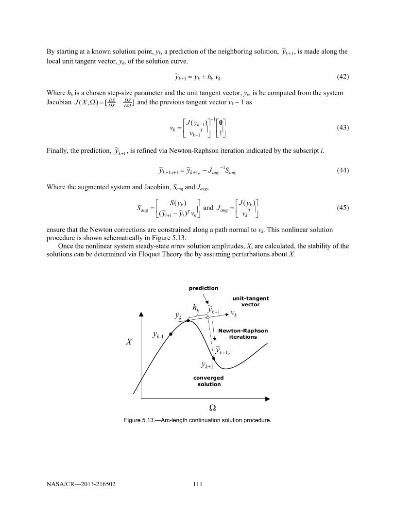
NASA/CR—2013-216502 111

By starting at a known solution point, yk, a prediction of the neighboring solution, 1~

+ky , is made along the local unit tangent vector, yk, of the solution curve.

kkkk vhyy ~1 +=+ (42)

Where hk is a chosen step-size parameter and the unit tangent vector, yk, is be computed from the system Jacobian ][),( Ω=Ω D

DSDXDSXJ and the previous tangent vector vk – 1 as

=

−

−

−

1)( 1

1

1 0T

k

kk v

yJv (43)

Finally, the prediction, 1~

+ky , is refined via Newton-Raphson iteration indicated by the subscript i.

augaugikik SJyy 1,11,1

~~ −+++ −= (44)

Where the augmented system and Jacobian, Saug and Jaug,

−

=+ k

Tii

kaug vyy

ySS

)~~()(

1 and

= T

k

kaug v

yJJ

)( (45)

ensure that the Newton corrections are constrained along a path normal to vk. This nonlinear solution procedure is shown schematically in Figure 5.13.

Once the nonlinear system steady-state n/rev solution amplitudes, X, are calculated, the stability of the solutions can be determined via Floquet Theory the by assuming perturbations about X.

Figure 5.13.—Arc-length continuation solution procedure.

X

Ω

yk

yk-1

yk+1

hk

prediction

unit-tangentvector

vk

Newton-Raphsoniterations

converged solution

1~

+ky

iky ,1~

+

NASA/CR—2013-216502 112

5.5.3 Dual Gearbox/Cross Shaft Response Results and Observations Utilizing the harmonic balance and continuation analysis methodology developed in the previous

section, the sTp period steady-state solutions are computed for a constant load torque level TL=100 N-m. Table 5.3 summarizes the dual gearbox/shaft system parameters utilized in this numerical investigation.

Figure 5.14 shows the resulting 1Tp, 2Tp and 3Tp period solutions versus operating speed for to values of gap clearance.

Here the effect of the tooth gap clearance is clear illustrated. For the case with no gap (i.e., the hgap=0 µm case), the response harmonics experience ordinary resonance-like behavior. However, once the backlash is included, (i.e., the hgap = 20 µm case), the response is significantly different. The presence of the gap clearance produces a softening “backbone” behavior of the resonance curve. This is a characteristic of a system which undergoes jump phenomena during spinup or spindown resulting in different limit cycle amplitudes depending on direction of the RPM change. Despite this behavior, backlash the nonlinearity has the beneficial effect of significantly reducing the vibration amplitudes compared with the hgap=0 µm case.

TABLE 5.3.—DUAL GEARBOX-SHAFT SYSTEM PARAMETERS

Parameter Value Number of teeth, Zi ............................................................ Z1=42, Z2 =30, Z3 =42, Z4=30 Pressure angle, αPA ..................................................................................................... 25° Circular pitch, cp ............................................................................................0.0157 m-1 Contact ratio, cr ..................................................................................................... 1.4954 Face width, d ......................................................................................................... 18 mm Gear Inertia, Ji ...................................... J1=0.243, J2 =0.063, J3 =0.234, J4=0.063 kg-m2 Load Inertia, JL ............................................................................................ JL=2.0 kg-m2 Load Torque, TL .................................................................................................. 500 Nm Backlash gap clearance, h ................................................................................. Various* Shaft Length, L ......................................................................................................... 10 m Shaft torsional stiffness, kt ................................................................................. Various* Density (shaft) ............................................................................................... 2800 kg/m3 Elastic modulus (gear), E ................................................................................... 200 GPa Shear modulus (shaft), G ...................................................................................... 27 GPa

*Various values used in the investigation

Figure 5.14.—Dual gearbox/shaft vibration response harmonics versus Ω with kt = 6000 Nm,

for two values of gap clearance; (a) hgap = 0 µm; (b) hgap = 20 µm.

500 1000 1500 2000 2500 3000 3500 40000

5

500 1000 1500 2000 2500 3000 3500 40000

0.5

1

1.5

500 1000 1500 2000 2500 3000 3500 4000

Ω, RPM

Period 1Tp

Period 2Tp

Period 3Tp

|u34|, µm

|u34|, µm

|u34|, µm

0

0.5

0.25

2.5

500 1000 1500 2000 2500 3000 3500 40000

5

500 1000 1500 2000 2500 3000 3500 40000

0.5

1

1.5

500 1000 1500 2000 2500 3000 3500 4000

Ω, RPM

Period 1Tp

Period 2Tp

Period 3Tp

|u34|, µm

|u34|, µm

|u34|, µm

0

0.5

0.25

0

0.5

0.25

2.5

NASA/CR—2013-216502 113

Figure 5.15.—Dual gearbox/shaft vibration response harmonics versus Ω with hgap = 20 µm

for; (a) kt = 6000 Nm; (b) kt = 2000 Nm; (c) kt = 1000 Nm.

Next, Figure 5.15 shows the effect of the dynamic mesh phase by comparing the dual gearbox/shaft system vibration response for three different shaft torsional stiffness values [kt = 6000 Nm, kt = 2000 Nm, and kt = 1000 Nm].

Here the effect of dynamic mesh phase is seen by the increased softening of the response backbone curves at each harmonic. To explore the onset of chattering behavior, the steady-state tooth impact velocities are plotted versus the shaft rotation speed in Figure 5.16. Tooth impact velocity cv is defined as the tooth velocity at the instant when either front-side or back-side tooth contact occurs. This is evaluated from time-domain simulation as

cttc uv

== with ε<− gapc htu )( (46)

where tc is the time of impact determined from the ε criteria in (46) where ε is small positive number. In this simulation the both gears pairs are operating in full contact for [1000 < Ω <1247] RPM. Above this threshold operating speed, chattering begins. In the range [1247 < Ω < 1328] RPM, the chattering response executes a 1Tp orbit. However over [1328 < Ω < 1823], the behavior appears chaotic. For [1823 < Ω < 2305] RPM, 2Tp behavior emerges with and 1Tp orbit reappearing for Ω > 2305 RPM.

Finally, Figure 5.17 shows the gear mesh deflection (13) vibration response of the dual gearbox/shaft systems during a [Ω = 3000 to 0 RPM] spindown for two shaft torsional stiffness values [kt = 15000 Nm and kt = 6000 Nm].

Here the increased shaft torsional flexibility (and increased dynamic mesh phase) has both stabilizing and destabilizing effects depending on the RPM range. Specifically, by comparing Figure 5.17(a) and (b), over the shaft speed range [Ω ≈ 1250 – 1700 RPM], the reduced shaft stiffness case (Figure 5.17(b)) tends to destabilize the higher amplitude 2Tp,limit cycle causing the response to jump down to the lower response amplitude 1Tp, limit cycle compared to the high torsion stiffness case (Figure 5.17(b)). However, the opposite behavior occurs over the shaft speed range [Ω ≈ 2400 – 2650 RPM]. In this range the response jumps from the 2Tp, limit-cycle to the higher amplitude 3Tp limit-cycle. Thus, the nonlinear dynamic mesh phasing effect between the upstream and downstream gearboxes, which is strongly related by the shaft torsional stiffness, is seen to have both beneficial and negative effects on the variable RPM torsional vibration response amplitudes.

500 1000 1500 2000 2500 3000 3500 40000

5

500 1000 1500 2000 2500 3000 3500 40000

0.5

1

1.5

500 1000 1500 2000 2500 3000 3500 4000

Ω, RPM

Period 1Tp

Period 2Tp

Period 3Tp

|u34|, µm

|u34|, µm

|u34|, µm

0

0.5

0.25

2.5

500 1000 1500 2000 2500 3000 3500 40000

5

500 1000 1500 2000 2500 3000 3500 40000

0.5

1

1.5

500 1000 1500 2000 2500 3000 3500 4000

Ω, RPM

Period 1Tp

Period 2Tp

Period 3Tp

|u34|, µm

|u34|, µm

|u34|, µm

0

0.5

0.25

0

0.5

0.25

2.5

NASA/CR—2013-216502 114

Figure 5.16.—Tooth impact velocity at steady-state versus shaft

speed; hgap = 20 µm; kt = 6000 Nm.

Figure 5.17.—Gear mesh vibration during shaft spindown from

[Ω = 3000 to 0 RPM]; with hgap = 20 µm for; (a) kt = 15000 Nm; (b) kt = 6000 Nm.

5.6 Summary and Conclusions

This section studies the nonlinear interactions between two gearboxes coupled by a torsionally flexible shaft. Such configurations are common in rotorcraft propulsion systems including tailrotor and cross-shafting drivelines. Shaft flexibility induces dynamic phasing between two coupled gearboxes. This dynamic phasing together with the kinematic dependence of the gear tooth mesh stiffness on the gear rotation induces a nonlinear dynamic interaction not explored in previous single-stage or rigid-shaft gear system investigations. The nonlinear time-varying equations-of-motion of a dual-spur gearbox/flexible

Chattering

Ω, RPM

Impa

ct v

eloc

ity, m

/s

One-sided impact(period 1Tp)

Double-sided impact(period 2Tp)Full contact

Chaotic

Chattering

Ω, RPM

Impa

ct v

eloc

ity, m

/s

Chattering

Ω, RPM

Impa

ct v

eloc

ity, m

/s

One-sided impact(period 1Tp)

Double-sided impact(period 2Tp)Full contact

Chaotic

NASA/CR—2013-216502 115

shaft system are derived via an assumed mode technique. Steady-state harmonic and subharmonic solutions are obtained via a harmonic balance and arc-length continuation strategy. Under zero backlash conditions, the dynamic mesh phase produces a softening-type nonlinearity in the resonance curves. Furthermore, under chattering conditions, increasing the shaft compliance tends to destabilize the single and double sided contact response amplitudes. The equations and analysis presented for the dual-gearbox shaft system demonstrate the importance of including nonlinear mesh phase interactions in multigearbox drive systems.

The equations and analysis presented for the dual-gearbox shaft system demonstrates the importance of including nonlinear mesh phase interactions in multigearbox drive systems. It is found that, similar to backlash effects, the mesh phase nonlinearity produces a softening-type resonance behavior. Furthermore, for higher load torque levels where gear chattering vibrations occur, reducing the intermediate shaft flexibility has the effect of destabilizing 2Tp solutions which naturally reduce the chattering response amplitudes over certain RPM ranges. This study also demonstrates the power and effectiveness of the harmonic balance and continuation approach for finding steady-state solutions to multiple degree-of-freedom nonlinear time-varying systems. One key factor is the location of the system structural modes in relation to the gear mesh harmonics. For variable speed operation, it is necessary to minimize the frequency crossings during spinup and spindown. When integer multiples of gear mesh frequency become close to structural modes involving gear mesh deflections chattering can occur. This chattering is exacerbated by the static load torque level. The analysis and results give insights into the relative importance of dynamic mesh phasing phenomena in multistage gear/shaft systems and should provide some design guidelines for flexible shaft/gearboxes systems.

NASA/CR—2013-216502 116

6.0 Two-Speed Dual Clutch Transmission 6.1 Introduction

Aircraft sizing design studies have identified that a two-speed rotor configuration is required (Refs. 1 and 104). Rotor speed at cruise is required to be reduced, possibly down to 50 percent of hover speed, to keep rotor blade advancing tip speeds reasonable. One early study of a multispeed rotorcraft drive system consisted of a high speed traction drive variator and a planetary differential gear unit (Ref. 4). A unit was tested and performed as designed. However, the mechanical efficiency was lower than that of a conventional drive system. Also, the use of traction drives for a main drive path is not an accepted practice for U.S. rotorcraft manufacturers. Previous studies have been sponsored by NASA to investigate multispeed drive systems (Refs. 3 and 105). These studies looked at earlier tiltrotor applications where 15 percent speed reduction for cruise was required. Dual path configurations and compound planetary configurations looked promising. However, a major concern of the shifting process as well as drive system weight penalties resulted from the studies. An electro-mechanical infinitely variable transmission, comprising a pair of planetary trains interconnected with two electric machines and clutches, has been proposed (Ref. 106). Again, the mechanical efficiency suffered as well as the added complexity of two planetary systems. A unique concept called a pericyclic continuously variable speed transmission is being investigated (Ref. 107). It uses pericyclic kinematics to achieve single speed reduction ratios between 1.05:1 to 50:1 with variable speed capability in one hardware stage. This concept, however, had yet to be tested. In summary, the results from the previous studies indicate that the incorporation of multispeed concepts in rotorcraft application is not a trivial process and adds complexity and weight. Thus, further research and development in this area is required, such as described in (Ref. 108). In addition, dynamic modeling of multispeed drive systems can help define the characteristics and limitations of the drive systems and the shifting process.

Since very few multispeed rotorcraft studies have been published, very little work on dynamic modeling for multispeed rotorcraft drive systems has been done. There has been, however, numerous publications on dynamic modeling of automotive drive systems. Much of the work addresses the automatic transmission shifting control with emphasis on maximizing fuel economy and maintaining performance (Refs. 109 to 115). For these, the typical system being modeled is the gasoline combustion engine, torque convertor, multispeed gearbox, tires and vehicle dynamics, as well as throttle and shifting controls. Dynamic speed, gear ratio, and torque are amongst the parameters predicted. This strategy has been applied to hybrid powertrains (Refs. 116 and 117), continuously variable transmissions (Refs. 118 to 121), and even heavy trucks and tanks for the military (Refs. 122 to 126). The modeling in the automotive field has had much success in improving drive train development. The approach and some modeling tools can be extended to the rotorcraft arena (Refs. 127 and 128). However, specifics of integration of the gas turbine engine, multispeed drive systems, clutches, and the dynamics of the rotor and rotorcraft vehicle have yet to been addressed in the rotorcraft application.

6.2 Two-Speed Dual Clutch Transmission In order to implement the variable speed rotorcraft driveline confutations, a two-speed Dual Clutch

Transmission (DCT) similar to that considered by Kish, 2002 is utilized in this study. Figure 6.1 shows the two-speed transmission considered in (Ref. 3) and Figure 6.2 shows the two-speed DCT considered in this study.

One key advantage of the DCT gearbox configuration is that it provides speed change via gear shifting though a split-path differential planetary arrangements. Here, in Figure 6.2, the high-speed ratio is accomplished by disengaging a ring clutch and engaging a set of planet clutches. For the low-speed ratio, the planet clutches are disengaged and the ring clutch is applied to lock the ring gear. In the low speed case, the power is split between two parallel paths which has the advantages of allowing an overall lower transmission weight. The corresponding kinematic diagram of the two-speed DCT in Figure 6.2 is shown in Figure 6.3.

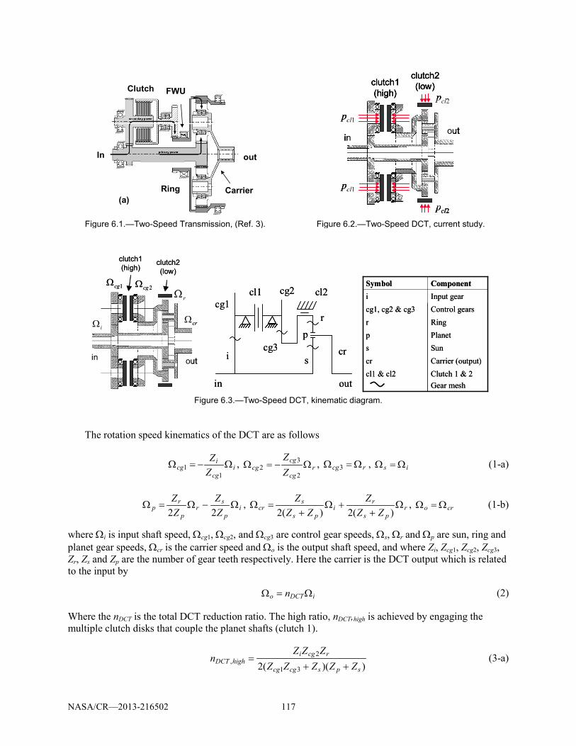
NASA/CR—2013-216502 117

Figure 6.1.—Two-Speed Transmission, (Ref. 3).

Figure 6.2.—Two-Speed DCT, current study.

Figure 6.3.—Two-Speed DCT, kinematic diagram.

The rotation speed kinematics of the DCT are as follows

icg

icg Z

ZΩ−=Ω

11 , r

cg

cgcg Z

ZΩ−=Ω

2

32 , rcg Ω=Ω 3 , is Ω=Ω (1-a)

ip

sr

p

rp Z

ZZZ

Ω−Ω=Ω22

, rps

ri

ps

scr ZZ

ZZZ

ZΩ

++Ω

+=Ω

)(2)(2, cro Ω=Ω (1-b)

where Ωi is input shaft speed, Ωcg1, Ωcg2, and Ωcg3 are control gear speeds, Ωs, Ωr and Ωp are sun, ring and planet gear speeds, Ωcr is the carrier speed and Ωo is the output shaft speed, and where Zi, Zcg1, Zcg2, Zcg3, Zr, Zs and Zp are the number of gear teeth respectively. Here the carrier is the DCT output which is related to the input by

iDCTo n Ω=Ω (2)

Where the nDCT is the total DCT reduction ratio. The high ratio, nDCT,high is achieved by engaging the multiple clutch disks that couple the planet shafts (clutch 1).

))((2 31

2,

spscgcg

rcgihighDCT ZZZZZ

ZZZn

++= (3-a)

(a)

Clutch

InIn out

CarrierRing

FWUclutch1 (high)

clutch2 (low)

inout

pcl2

pcl1

pcl1

pcl2

clutch1 (high)

clutch2 (low)

inout

pcl2

pcl1

pcl1

pcl2

clutch1 (high)

clutch2 (low)

inout

pcl2

pcl1

pcl1

pcl2

clutch1 (high)

clutch2 (low)

in out

crΩ

1cgΩ

iΩ

rΩ2cgΩ

clutch1 (high)

clutch2 (low)

in out

crΩ

1cgΩ

iΩ

rΩ2cgΩ

cl1

s

cg1cg2

cg3 cri

in out

pr

cl2cl1

s

cg1cg2

cg3 cri

in out

pr

cl2

Clutch 1 & 2Gear mesh

cl1 & cl2Carrier (output)crSunsPlanetpRingrControl gearscg1, cg2 & cg3Input geariComponentSymbol

Clutch 1 & 2Gear mesh

cl1 & cl2Carrier (output)crSunsPlanetpRingrControl gearscg1, cg2 & cg3Input geariComponentSymbol

NASA/CR—2013-216502 118

Furthermore, low ratio, nDCT,low, is achieved by fully engaging, the cylindrical ring clutch (clutch 2) which clamps the ring gear.

)(2,

sp

slowDCT ZZ

Zn+

= (3-b)

Clutch engagement is controlled by applied pressures, pcl1 and pcl2, normal to the clutch fiction surfaces. Due to the DCT kinematics, the only condition under which both sets of clutches can be engaged and locked simultaneously corresponds to the zero speed or fully stalled condition. When both clutches are applied simultaneously there is a negative recirculating power ratio and clutches act as a braking system. Thus, during steady-state constant speed operation, only one clutch is fully engaged and locked (with maximum applied clutch pressure pcli = pclmax) while the other clutch remains open (with no applied clutch pressure pclj = 0). The parameters of the two-speed DCT utilized in this study are summarized in Table 6.1.

TABLE 6.1.—TWO-SPEED DUAL CLUTCH TRANSMISSION PARAMETERS

Parameter Value Number of gear teeth .............................................................................. Zi=40, Zcg1=42, Zcg2=29, Zcg3=52, Zr=74, Zp=14, Zs=46 Gear radii, m ............................................ Ri=0.1, Rcg1=0.106, Rcg2=0.074, Rcg3=0.132, Rr=0.19, Rp=0.036, Rs=0.12, Rcr=0.152 Rotational inertias, kg m2 ...................... Ji=0.064, Jcg1=0.078, Jcg2=0.039, Jcg3=0.402, Jr=1.766, Jp=0.002, Js=0.264, Jcr=0.848 Number of planets .............................................................................................................................................................. Np = 8 Planet mass, kg ............................................................................................................................................................mp = 3.576 Planet clutch radius (clutch 1), m ............................................................................................................................. Rc11 = 0.238 Number of planet clutches (clutch 1) ............................................................................................................................... Ncg = 2 Ring clutch dimensions (clutch 2), m ....................................................................................................... Rc12 = 0.197, Lc12 = 0.1 Clutch friction coefficient ............................................................................................................................................ µcl = 0.45 Clutch viscous torque parameter, N m sec ................................................................................................................. τcl = 1×102

Based on these parameters, the low ratio is 383.0, =lowDCTn and the high ratio is 711.0, =highDCTn which means about 47 percent speed reduction from the high to the low ratio.

6.3 Dual Clutch Transmission Dynamics Model

To account for the DCTs in the driveline simulation, a rigid body dynamics model is developed which accounts for the DCT kinematics, the gear rotational inertias, and the nonlinear clutch friction torques. The equations of motion have the form

),,( 21 clcl ppΩFΩM = (4-a)

with corresponding angular velocity degrees-of-freedom

Tri ttt )]( ),([)( ΩΩ=Ω (4-b)

consisting of the DCT input and ring gear rotation speeds. Also, the system inertia matrix is

NASA/CR—2013-216502 119

+

+++

+++

−

+++

−

+++

+

+++

++++

=

22

22

22

232

3

22

2

22

2

22

22

21

21

)(4

)(4

)(4

)(4

p

pp

sp

crppoutcrr

cg

cgcgcgcgr

p

pp

sp

crppoutcrsr

p

pp

sp

crppoutcrsr

p

pp

sp

crppoutcrs

cg

icgcgsiin

ZNJ

ZZRmNJJZ

ZZNJ

JJ

ZNJ

ZZRmNJJZZ

ZNJ

ZZRmNJJZZ

ZNJ

ZZRmNJJZ

ZZNJ

JJJ

M (4-c)

and the system generalized force vector is

1

0

)(20

)(21

),,(2

1

2

3

121

−

−

+

+−+

−

=cl

cl

cg

cgcg

cg

icg

o

i

sp

r

sp

s

clcl ΓΓ

ZZN

ZZN

ΓΓ

ZZZ

ZZZ

ppΩF (4-d)

Where Γi and Γo are input and output shaft the torques on the DCT and where Γcl1 and Γcl2 are the transmitted clutch torques which are computed based on a combined Coulomb/viscous model (Refs. 127, 129 and 130

≥Ω−ΩΩ−Ω

<Ω−ΩΩ−Ω=

(slipping) when )sgn(3

4(sticking) en wh )(

1212

31

1

1212

1επµ

ετ

cgcgcgcgcl

clcl

cgcgcgcgcl

cl RpΓ (5-a)

≥ΩΩ<ΩΩ

=(slipping) when )sgn(2

(sticking) n whe

22

222 επµ

ετ

rrclclclcl

rrclcl LRpΓ (5-b)

Here µcl and τcl are clutch friction and viscous torque coefficients (Ref. 129). Note, clutch 1 is a disk-type clutch therefore 1clΓ is a function of disk radius Rc11, and clutch 2 is a cylindrical ring clutch thus 2clΓ depends on clutch radius, Rc12, and axial length Lc12. This nonlinear torque model accounts for the possibility of clutch sticking (lockup) and slipping.

In this clutch model, (5), the individual clutch torques, cliΓ , transition between viscous (sticking) mode and Coulomb friction (slipping) mode based on the clutch slip-speed threshold which is evaluated at each simulation time-step. The slip-speed threshold parameter, ε, is a small positive number in the simulation. If the clutch slip-speed exceeds ε then the torque transitions from sticking to slipping mode. Likewise, if clutch slip-speed drops below ε then the clutch torque transitions back to sticking mode. By proper selection of ε and τcl, the viscous mode numerically approximates clutch lockup without no need for explicit kinematic constraints or model DOF reduction (Ref. 127). The DCT system parameters used in this investigation are summarized in Table 6.1. Also, it is important to note that the clutch torque, cliΓ , depends on the applied pressure clutch pcli only during the slipping mode.

Figure 6.4 shows the Matlab Simulink block diagram representation of the dual clutch DCT system utilized in the comprehensive simulation models presented in Section 7.0. Here the saturation blocks are utilized to allow the transition from sticking to slipping torque modes.

NASA/CR—2013-216502 120

Figure 6.4.—Two-Speed DCT dynamics model.

Planet Clutch (Clutch #1)

Ring Clutch (Clutch #2)

Clutch #1 Torque

Clutch #2 Torque

Clutch #1Input

pressure

Clutch #2Input

pressure

1cgΩ

2cgΩ

rΩ

iΩ

oΩ

1clΓ

2clΓ

Zs

Zr

Planet Clutch (Clutch #1)

Ring Clutch (Clutch #2)

Clutch #1 Torque

Clutch #2 Torque

Clutch #1Input

pressure

Clutch #2Input

pressure

1cgΩ

2cgΩ

rΩ

iΩ

oΩ

1clΓ

2clΓ

Zs

Zr

NASA/CR—2013-216502 121

7.0 Comprehensive Variable Speed Rotorcraft Propulsion System Model and Simulation

7.1 Introduction

One of the main goals of this research project is to develop a comprehensive first principles-based drive-system modeling tool to predict the complex transient dynamic response of variable speed rotorcraft propulsion systems including engine, transmission, clutch, cross-shafting, and rotor dynamic interactions. By accounting for the various propulsion subsystem dynamic interactions, this new Comprehensive Variable Speed Rotorcraft Propulsion System Modeling (CVSRPM) tool enables performance prediction to give future design insights and enable system level understanding.

Furthermore, another goal is to exercise this newly developed computational tool to explore the behavior of various variable ratio rotorcraft drive-system configurations and ratio changing strategies under simulated operational conditions. To address these goals, a comprehensive rotorcraft propulsion system simulation tool based on the subsystem models developed in Sections 2.0 to 6.0 is constructed. Simulations are then performed for several different drive system configurations to evaluate their variable speed performance characteristics.

7.2 Variable Speed Rotorcraft Propulsion System Model

The comprehensive dynamic simulation tool assembled in this project is based combining several of the key rotorcraft driveline subsystem models developed for in Sections 2.0 to 6.0. Figure 7.1 shows as schematic of the overall CVSRPM architecture along with the various subsystem model interaction paths. For reference, Figure 7.1 also gives the corresponding section number of the particular subsystem model when appropriate. Specifically, the main elements and assumptions included in this comprehensive, variable speed, drive system simulation tool are as follows

• Two-spool gas turbine engine transient dynamics model and closed-loop PID fuel controller to

regulate power turbine speed (Section 6.0). • Dual-Clutch Transmission (DCT) gearbox model with stick-slip friction and clutch lockup effects

(from Section 6.0). • Simplified main rotor model based on momentum theory (from Section 2.0) • Torsionally flexible shafting and cross-shafts (misalignment and bending not considered) • All rigid gearing (tooth mesh compliance and mesh stiffness variations neglected) • A two DOF flight dynamics model for fuselage drag, vehicle forward flight and elevation

dynamics with vehicle states [ yy,,xx, ]. • A PID based main rotor blade pitch controller to regulate rotor thrust to track a desired forward

speed setpoint (controls main rotor pitch θpitch) • A PID based wing elevon pitch controller to maintain level flight or track a desire climb rate

setpoint (controls wing flap angle θwing) The comprehensive dynamic simulation code is implemented under the Matlab Simulink software

environment. Here, each subsystem block of the CVSRPM code as shown in Figure 7.1 is detailed in the Appendix.

NASA/CR—2013-216502 122

Figure 7.1.—Comprehensive Variable Speed Rotorcraft Propulsion System Model.

Due to the inherently high frequency nature of the gear mesh stiffness variation and backlash effects

(as is considered in Section 5.0), difficulties related to excessive simulation times and storage space were encountered when these effects were included in the comprehensive simulation model. For example, the first fundament drive system torsion mode is typically on the order of 1 to 5 Hz while the gear mesh stiffness variations may be on the order of 5000 Hz, thus requiring excessively small numerical integration time-steps compared to the overall drive-system maneuver timescales. Here, the decision was made to neglect the gear mesh effects in the comprehensive simulation model and consider rigid gearing to reduce the simulation runtimes and data storage requirements. Apart from these issues, the simulations can be run within a “reasonable” about of time on a modern PC or notebook computer. For example, for a typical dual-path drive system (tiltrotor) performing an upshift followed by a downshift maneuver over a simulated time span of 280 sec, the simulation can be can be completed in approximately 15 min of CPU execution time. In the subsequent sections, several two-speed gear change maneuvers for a single-path and dual-path rotorcraft drive system configuration is explored using the CVSRPM code.

7.3 Two-Speed Shift Rotorcraft Drive-System Case Studies In this section, the newly developed CVSRPM code is used to investigate the variable speed

operational behavior of two different rotorcraft drive system configurations each equipped with two speed dual clutch transmissions (see Section 4.0). Here both the conventional helicopter and the tiltrotor drive-system configurations are considered. In each case, the system executes a fully trimmed simulated in-flight maneuver as regulated by the three different closed-loop control systems (i.e., the engine fuel control, blade pitch forward speed control, and the auxiliary wing lifting surface controller). During flight, open-loop clutch shift commands are applied to the dual-clutch gearbox transmission(s) and the resulting variable speed system response is computed.

NASA/CR—2013-216502 123

7.3.1 Two-Speed Helicopter Drive System Figure 7.2 gives a schematic of the two-speed helicopter drive system simulation model implemented

with the CVSRPM code. In this helicopter drive system there are three reduction stages from the power turbine speed Ωpt to the

main rotor speed ΩMR.

ptiDCTfMR nnn Ω=Ω (1)

Here ni is the initial reduction ratio, nDCT is the DCT reduction ratio (see Section 4.0) and nf is the final reduction.

In this analysis, the variable rotor speed propulsion system response is computed for the helicopter in a hover condition. The free-body-diagram of the simplified hover model is shown in Figure 7.3 and the hover flight dynamics model is given by Equation (2).

gmvFym vvpitchMRTv −Ω= ),,( θ with yvv = (2)

Where mv is vehicle mass, g is acceleration of gravity, y is vertical position coordinate of the vehicle mass center, vv is vehicle vertical speed, and FT is main rotor thrust. Here FT is a function of main rotor speed, ΩMR, main rotor blade pitch, θpitch, and vv. The main rotor thrust computation is shown in Section 2.5. In this study, the parameters for the hypothetical two-speed rotor helicopter system are based on a CH-53 helicopter platform (Ref. 131). All of the helicopter system parameters used in this study are given in Table 2.3, Table 4.1, Table 4.3, Table 6.1, Table 7.1, and Table 7.2.

Figure 7.2.—Two-speed helicopter drive system simulation model.

Figure 7.3.—Helicopter hover flight dynamics

FWU

FWU

Gas Turbine Engines

Two Speed Dual Clutch

Transmission(DCT)ni

nf

Final RatioInitial

Ratio

Main Shaft

Main Rotor

High Speed Clutch

Low Speed Clutch

ΩMR

TMR

JMR

ClutchEngagement

Pressure Inputs

Blade Pitch Controlfor Hover

θpitchFuel Control

fm

vv,setΩpt,set

FWU

FWU

Gas Turbine Engines

Two Speed Dual Clutch

Transmission(DCT)ni

nf

Final RatioInitial

Ratio

Main Shaft

Main Rotor

High Speed Clutch

Low Speed Clutch

ΩMR

TMR

JMR

ClutchEngagement

Pressure Inputs

Blade Pitch Controlfor Hover

θpitchFuel Control

fm

vv,setΩpt,set

gmv

TFpitchθ

yPID

vv

setvv−

Blade Pitch Control

gmv

TFpitchθ

yPIDPID

vv

setvv−

Blade Pitch Control

NASA/CR—2013-216502 124

TABLE 7.1.—HELICOPTER PARAMETERS Parameter Value Vehicle mass, mv .......................................................... 20,865 kg Initial ratio, ni .................................................................... 0.5347 Final ratio, nf ......................................................................... 0.04

Figure 7.4.—Blade pitch control block diagram.

In order to maintain hover with a desired vertical speed setpoint, setvv , blade pitch is regulated with a

PID-based blade pitch controller of the form

vdvIvppitch ekdtekekppp++= ∫θ with vvv vve

set−= (3)

With blade pitch control gains ppk , pIk and pdk , to regulate the setpoint speed error ve . It is also

necessary to account for the physical blade pitch limits minpitchθ and maxpitchθ which is accomplished through use of a saturation block and back-calculating gain,

pbk , to prevent integrator windup. Figure 7.4 shows a block diagram of the blade pitch control.

The gains ppk ,

pIk and pdk were selected by trial-and-error until a stable closed-loop system was

achieved. The blade pitch control system parameters are shown in Table 7.2.

TABLE 7.2.—HELICOPTER BLADE PITCH CONTROL SYSTEM PARAMETERS

Parameter Value Proportional gain,

ppk ........................................ 0.004 rad-sec/m

Integral gain, pIk ...................................................... 0.005 rad/m

Derivative gain, pdk ...................................... 4.0×10-5 rad-sec2/m

Back-calculating gain, pbk ............................................. 100 sec-1

Minimum blade pitch, minpitchθ ................................................... 0°

Maximum blade pitch, maxpitchθ ................................................ 17°

PIDPID

NASA/CR—2013-216502 125

Figure 7.5.—Main rotor downshift/upshift during hover.

The first variable rotor speed mission profile studied is a main rotor downshift/upshift procedure

during hover conditions. This variable rotor RPM maneuver consists of a downshift followed by an upshift, all during hover with a zero vertical speed setpoint, 0=

setvv kn, as shown in Figure 7.5. The resulting system response is detailed in Figure 7.6 to Figure 7.9. Here the helicopter is initially

operating at 100 percent rotor speed, then, at t = 40 sec, the downshift is initialed. The high-speed clutch axial engagement pressure is commanded to ramp-down while the low-speed clutch pressure (originally disengaged) is simultaneously commanded to ramp-up. The pressures are commanded to keep increasing (or decreasing) until clutch becomes fully locked (or fully disengaged). The clutch command engagement pressures are plotted in Figure 7.6(c).

Figure 7.6(b) shows corresponding response of the main rotor speed which shows an essentially linear decrease in rotor RPM until the low-speed clutch becomes locked. Then a very slight RPM dip is observed immediately after lockup which is due to system torsional compliances. Furthermore, Figure 7.6(a) shows the engine power turbine speed which is strongly influenced the choice of PID fuel control gains (see Section 4.0). Next at t = 80 sec, the upshift command is initiated. Here the process is essentially the revere of the downshift and the corresponding rotor speed and engine speed responses are also well behaved.

Still more insight is gained by examining Figure 7.7, which shows the system torque responses. Here it is observed that the main rotor torque (Figure 7.7(a)) actually increases as a result of the lower rotor RPM. At first pass this seems counter intuitive, however, the rotor torque increase is a result of the pitch controller trying to maintain a constant rotor thrust in order to maintain the hover. As the rotor RPM drops, the pitch controller must add more collective blade pitch to generate the thrust, thereby increasing the rotor drag torque. The blade pitch control input is shown in Figure 7.9(c).

Next the, engine output torque, shown in (Figure 7.7(b)), is also seen to significantly rise during both the downshift and the upshift events. Due to the magnitude of the engine torque increase, this cannot be explained by the effect of the main rotor blade pitch control. Rather, it is the result of the opposing split path power flows inside the DCT gearbox. For the applied shift command inputs (Figure 7.6(c)), both the high and low speed clutches are simultaneously engaged and slipping during up and downshifts. The resulting re-circulating power must be counteracted by the engines. However, it is this same effect which enables the smooth, linear rotor speed transitions observed in Figure 7.6(b). Without some level of clutch overlap and power re-circulation, the rotor RPM may go into a neutral condition and lose speed rapidly. This is further illustrated by observing the transmitted clutch torques in Figure 7.7(c). Here, also high frequency stick-slip torque oscillations are observed in the low-speed clutch during its disengagement. Also Figure 7.8 shows the corresponding clutch power dissipated during the shift. Here again both clutches dissipate heat during the transitions but then, of course, the power dissipation is zero after it either becomes fully locked or fully disengaged. It is also interesting to observe that the power dissipated during the downshift is significantly more than during the rotor upshift. One explanation for this is that a significant portion of the main rotor’s kinetic energy is being dissipated by the clutches during the rotor speed downshift. Likewise, during upshift, power is flowing into the rotor. Here again, it is all down to choice of shift command inputs or shift strategy. If the rotor was allowed to go into a pure neural condition it would naturally execute a decrease in RPM due the rotor drag torque, with zero power dissipated in the clutches. However, the designer must find the correct balance between clutch overlap (with smooth ratio changes) and a neutral drop (no clutch heating but less rotor RPM control during shifts).

ΩMR

time

Main Rotor Speed

190 RPM

117 RPM

vv,set

Climb SetpointSpeed 0 knots(a)

(b)

ΩMR

time

Main Rotor Speed

190 RPM

117 RPM

vv,set

Climb SetpointSpeed 0 knots(a)

(b)

NASA/CR—2013-216502 126

Finally Figure 7.9 summarizes the corresponding helicopter flight parameters during the hover downshift/upshift simulation. Here, it is seen that the rotor downshift and upshift causes minimal disturbances to the vertical speed and accelerations (Figure 7.9(b)).

Figure 7.6.—Two-speed helicopter drive-system response for

downshift/upshift during hover; (a) engine power turbine response; (b) main rotor speed; (c) clutch engagement pressures

Figure 7.7.—Two-speed helicopter drive-system response for

downshift/upshift during hover; (a) main rotor torque; (b) engine output torque; (c) clutch torques.

Power Turbine Speed

Rotor Speed

Shift Command

time, sec

20 40 60 80 100 12011121314

kRPM

20 40 60 80 100 1200

100

200

RPM

20 40 60 80 100 1200

50

100

psi

(a)

(b)

(c)

Downshift Upshift

Low Speed Clutch

High Speed Clutch

Power Turbine Speed

Rotor Speed

Shift Command

time, sec

20 40 60 80 100 12011121314

kRPM

20 40 60 80 100 1200

100

200

RPM

20 40 60 80 100 1200

50

100

psi

(a)

(b)

(c)

Downshift Upshift

Low Speed Clutch

High Speed Clutch

20 40 60 80 100 1200

50010001500

TQ, k

Nm

20 40 60 80 100 1200

5

10

Te (n

acel

le),

kNm

20 40 60 80 100 120-50

0

50

Tc, k

Nm

Rotor Torque

Engine Torque

Clutch Torques

(a)

(b)

(c)

Downshift Upshift

time, secSlick-slip oscillations

20 40 60 80 100 1200

50010001500

TQ, k

Nm

20 40 60 80 100 1200

5

10

Te (n

acel

le),

kNm

20 40 60 80 100 120-50

0

50

Tc, k

Nm

Rotor Torque

Engine Torque

Clutch Torques

Rotor Torque

Engine Torque

Clutch Torques

(a)

(b)

(c)

Downshift Upshift

time, secSlick-slip oscillations

NASA/CR—2013-216502 127

Figure 7.8.—Two-speed helicopter drive-system response for

downshift/upshift during hover; (a) clutch torques; (b) clutch power dissipation.

Figure 7.9.—Two-speed helicopter drive-system response for downshift/upshift

during hover; (a) vertical speed; (b) vertical acceleration; (c) blade pitch input. (d) rotor induced flow.

7.3.2 Two-Speed Tiltrotor Driveline System As mentioned in References 1, 3, and 104, one of the potential beneficiaries of variable speed rotor

drive-system technologies is in the area of Heavy-Lift helicopter and tiltrotor configurations. Therefore, the next case explored using the CVSRPM simulation code is a tiltrotor configuration based on the NASA LCTR-2 Civil Tiltrotor shown in Figure 7.10 (Ref. 104).

Specifically, Figure 7.11 is the schematic of the two-speed tiltrotor drive-system simulation model implemented with the CVSRPM code.

20 40 60 80 100 120-50

0

50

Tc, k

Nm

20 40 60 80 100 120

0

2000

4000

Pc,

Hp

time, sec

Clutch Torque

Clutch Power

(a)

(b)

Downshift Upshift

20 40 60 80 100 120-50

0

50

Tc, k

Nm

20 40 60 80 100 120

0

2000

4000

Pc,

Hp

time, sec

Clutch Torque

Clutch Power

(a)

(b)

Downshift Upshift

Vertical Acceleration

20 40 60 80 100 120

-2

2

knts

20 40 60 80 100 120-0.1

0

0.1

g

20 40 60 80 100 12048

1216

deg

20 40 60 80 100 1200

12

m/s

Vertical Speed

Blade Collective

Pitch

Induced Inflow

time, sec

(a)

(b)

(c)

(d)

Downshift Upshift

Vertical Acceleration

20 40 60 80 100 120

-2

2

knts

20 40 60 80 100 120-0.1

0

0.1

g

20 40 60 80 100 12048

1216

deg

20 40 60 80 100 1200

12

m/s

Vertical Speed

Blade Collective

Pitch

Induced Inflow

time, sec

(a)

(b)

(c)

(d)

Downshift Upshift

NASA/CR—2013-216502 128

Figure 7.10.—NASA Large Civil Tiltrotor LCTR-2 (Ref. 104).

Figure 7.11.—Two-speed tiltrotor dual path driveline simulation model.

In each branch of the dual path tiltrotor driveline there are three reduction stages from the power

turbine to the main rotor. Here ni is the initial reduction, nDCT is the DCT reduction ratio (see Section 6.0) and nf is the final reduction stage. Furthermore, as shown in Figure 7.11, the left and right branches of the drive-system are linked via a cross-shaft. In this analysis, the cross-shaft is considered to be torsionally flexible with torsional stiffness kcs. This dual path driveline is implemented in the CVSRPM code by utilizing two identical single path drivelines similar to the conventional helicopter and then linking them via a torsional spring element to simulate the cross-shaft.

FWU

FWU

FWU

FWU

Right Nacelle(Twin Two Spool Gas

Turbine Engines)

Left Nacelle(Twin Two Spool Gas

Turbine Engines)Initial

Ratio, ni Final Ratio, nf

ForwardSpeed

Blade PitchControl

Multi-EngineFuel Control

Initial Ratio, ni

Final Ratio, nf

Left Rotor

Right Rotor

Dual Clutch TransmissionnDCT,low &nDCT,high

Clutch Engagement

Pressure Inputs

Dual Clutch TransmissionnDCT,low &nDCT,high

Cross-Shaft

1:1

1:1

setptΩsetcv

FWU

FWU

FWU

FWU

Right Nacelle(Twin Two Spool Gas

Turbine Engines)

Left Nacelle(Twin Two Spool Gas

Turbine Engines)Initial

Ratio, ni Final Ratio, nf

ForwardSpeed

Blade PitchControl

Multi-EngineFuel Control

Initial Ratio, ni

Final Ratio, nf

Left Rotor

Right Rotor

Dual Clutch TransmissionnDCT,low &nDCT,high

Clutch Engagement

Pressure Inputs

Dual Clutch TransmissionnDCT,low &nDCT,high

Cross-Shaft

1:1

1:1

FWU

FWU

FWU

FWU

Right Nacelle(Twin Two Spool Gas

Turbine Engines)

Left Nacelle(Twin Two Spool Gas

Turbine Engines)Initial

Ratio, ni Final Ratio, nf

ForwardSpeed

Blade PitchControl

Multi-EngineFuel Control

Initial Ratio, ni

Final Ratio, nf

Left Rotor

Right Rotor

Dual Clutch TransmissionnDCT,low &nDCT,high

Clutch Engagement

Pressure Inputs

Dual Clutch TransmissionnDCT,low &nDCT,high

Dual Clutch TransmissionnDCT,low &nDCT,high

Clutch Engagement

Pressure Inputs

Dual Clutch TransmissionnDCT,low &nDCT,high

Cross-Shaft

Cross-Shaft

1:1

1:1

setptΩsetcv

NASA/CR—2013-216502 129

In this study, variable rotor speed operation is analyzed for the tiltrotor operating in forward flight airplane mode as shown in Figure 7.12. Furthermore, the forward flight dynamics model of the tiltrotor is given by Equation (4).

xv

gmvFymvFvFxm

c

vcwingLv

wingcDcpitchMRTv

=

−=

−Ω=

),(),(),,(2

θθθ

(4)

Where x and y are horizontal and vertical vehicle position coordinates. FT is main rotor thrust, FD is vehicle aerodynamic drag and FL is the total wing lift force. In the tiltrotor case, FT is computed according to Section 2.5 and is a function of main rotor speed, ΩMR, main rotor blade pitch, θpitch, and forward speed vc. The lift a drag forces are computed as

2

2 cLwair

L vcAF ρ= and 2

2 cDwair

D vcAF ρ= (5)

Where airρ is air density, wA is total wing lift area and Lc and Dc are wing lift and drag coefficients respectively. Finally, the wing lift coefficient is computed in terms of the wing flap pitch wingθ as

wingLL cc θα= (6)

Where αLc is wing lift coefficient slope. The tiltrotor system parameters assumed in this investigation are based on the NASA LCTR-2 (Ref. 104). All of the tiltrotor system parameters used in this study are given in Table 2.4, Table 4.1, Table 4.3, Table 6.1, Table 7.3, Table 7.4, and Table 7.5.

Figure 7.12.—Tiltrotor forward flight airplane mode flight dynamics.

θwingθpitch

PID

PID

θpitch

TF

TF

DF

gmv

LFy

x

θwingθpitch

PIDPIDPID

PIDPIDPID

θpitch

TF

TF

DF

gmv

LFy

x

NASA/CR—2013-216502 130

TABLE 7.3.—TILTROTOR PARAMETERS Parameter Value Vehicle mass, vm .......................................................... 48762 kg Initial ratio, in ................................................................... 0.5347 Final ratio, fn ....................................................................... 0.04 Cross-shaft torsional stiffness, kcs ............................... 21219 N m Wing lift coefficient slope, αLc ................................ 12.578 rad-1 Vehicle drag coefficient, Dc ............................................... 0.054 Wing lift area, wA ......................................................... 93.04 m2

In order to maintain forward flight two PID control loops are utilized. The first control loop adjusts

main rotor pitch pitchθ to maintain a forward speed setpoint setcv See Figure 7.4 for a block diagram.

vdvIvppitch ekdtekekppp++= ∫θ with ccv vve

set−= (7)

The other control loop adjusts wing flap angle wingθ to maintain a vertical speed setpoint setvv . For level flight setvv = 0.

vdvIvpwing ekdtekekwww++= ∫θ with vvv vve

set−= (8)

Similar to the rotor pitch control, the wing flap control also utilizes a saturation block and a back-calculating gain,

wbk , to account for the wing pitch limits. Figure 7.13 shows the wing pitch control block diagram.

The wing and pitch control gains were selected by trial-and-error until a stable closed-loop system was achieved. The blade and wing pitch control system parameters for the tiltrotor are given in Table 7.4 and Table 7.5.

Figure 7.13.—Wing pitch control block diagram.

PIDPID

NASA/CR—2013-216502 131

TABLE 7.4.—TILTROTOR BLADE PITCH CONTROL SYSTEM PARAMETERS

Parameter Value Proportional gain,

ppk ......................................... 0.004 rad-sec/m

Integral gain, pIk ...................................................... 0.005 rad/m

Derivative gain, pdk ...................................... 4.0×10-5 rad-sec2/m

Back-calculating gain, pbk ............................................. 100 sec-1

Minimum blade pitch, minpitchθ ...................................................0°

Maximum blade pitch, maxpitchθ ................................................80°

TABLE 7.5.—TILTROTOR WING PITCH

CONTROL SYSTEM PARAMETERS Parameter Value Proportional gain,

wpk .............................................0.1 rad-sec/m

Integral gain, wIk ........................................................ 0.05 rad/m

Derivative gain, wdk ............................................ 0.02 rad-sec2/m

Back-calculating gain, wbk .............................................. 1.0 sec-1

Minimum wing pitch, minwingθ ................................................... 0°

Maximum wing pitch, maxwingθ ................................................ 10°

Figure 7.14.—Variable rotor speed tiltrotor mission profiles; (a) steady forward cruise downshift/upshift; (b) variable

forward cruise downshift/upshift. Another factor which becomes important in coupled multipath drive-systems is component

dissimilarly. In the tiltrotor case (Figure 7.14), if each component is identical with symmetric rotor loads, then the cross-shaft torque is zero and there will be no interactions between the two drive-system paths. In the case of the two-speed tiltrotor configuration, one unique and potentially significant source of component dissimilarly is with the clutches. Differences in clutch frictional characteristics between the left and right-side tiltrotor driveline branches could result in clutch torque interactions across the cross-shaft during shift events. To assess this possibility, a 1 percent dissimilarly between the left and right side DCT clutch friction coefficients µcl is assumed in the analysis.

The simulated mission profiles considered in this investigation for the variable rotor speed tiltrotor are shown in Figure 7.14.

Forward Speed

Setpoint

Main Rotor Speed

ΩMR

time

190 RPM

102 RPM

300 knots

150 knotssetcv

Climb rate

Setpoint

0 knotssetvv

(b)

Main Rotor Speed

Forward Speed

Setpoint

ΩMR

time

190 RPM

102 RPM

setcv

Climb rate

Setpoint

0 knotssetvv

(a)

225 knotsForward Speed

Setpoint

Main Rotor Speed

ΩMR

time

190 RPM

102 RPM

300 knots

150 knotssetcv

Climb rate

Setpoint

0 knotssetvv

(b)

Forward Speed

Setpoint

Main Rotor Speed

ΩMR

time

190 RPM

102 RPM

300 knots

150 knotssetcv

Climb rate

Setpoint

0 knotssetvv

(b)

Main Rotor Speed

ΩMR

time

190 RPM

102 RPM

300 knots

150 knotssetcv

Climb rate

Setpoint

0 knotssetvv

(b)

Main Rotor Speed

Forward Speed

Setpoint

ΩMR

time

190 RPM

102 RPM

setcv

Climb rate

Setpoint

0 knotssetvv

(a)

225 knots

Main Rotor Speed

Forward Speed

Setpoint

ΩMR

time

190 RPM

102 RPM

setcv

Climb rate

Setpoint

0 knotssetvv

(a)

225 knots

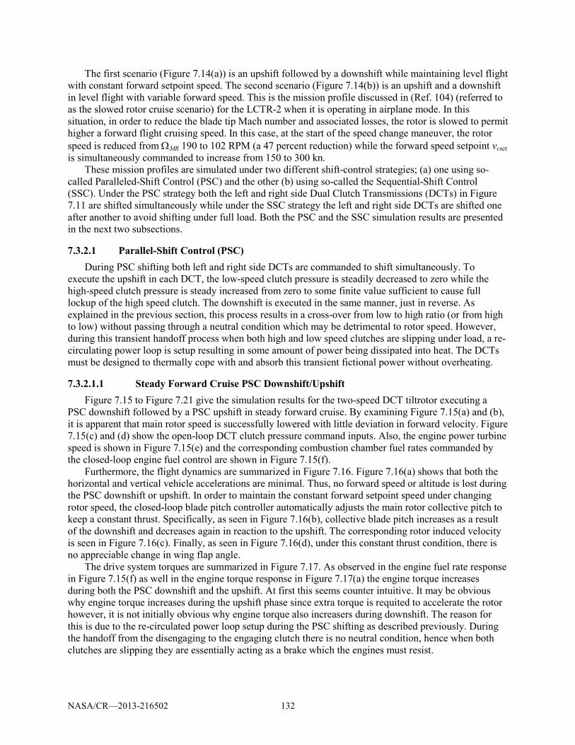
NASA/CR—2013-216502 132

The first scenario (Figure 7.14(a)) is an upshift followed by a downshift while maintaining level flight with constant forward setpoint speed. The second scenario (Figure 7.14(b)) is an upshift and a downshift in level flight with variable forward speed. This is the mission profile discussed in (Ref. 104) (referred to as the slowed rotor cruise scenario) for the LCTR-2 when it is operating in airplane mode. In this situation, in order to reduce the blade tip Mach number and associated losses, the rotor is slowed to permit higher a forward flight cruising speed. In this case, at the start of the speed change maneuver, the rotor speed is reduced from ΩMR 190 to 102 RPM (a 47 percent reduction) while the forward speed setpoint vcset is simultaneously commanded to increase from 150 to 300 kn.

These mission profiles are simulated under two different shift-control strategies; (a) one using so-called Paralleled-Shift Control (PSC) and the other (b) using so-called the Sequential-Shift Control (SSC). Under the PSC strategy both the left and right side Dual Clutch Transmissions (DCTs) in Figure 7.11 are shifted simultaneously while under the SSC strategy the left and right side DCTs are shifted one after another to avoid shifting under full load. Both the PSC and the SSC simulation results are presented in the next two subsections.

7.3.2.1 Parallel-Shift Control (PSC) During PSC shifting both left and right side DCTs are commanded to shift simultaneously. To

execute the upshift in each DCT, the low-speed clutch pressure is steadily decreased to zero while the high-speed clutch pressure is steady increased from zero to some finite value sufficient to cause full lockup of the high speed clutch. The downshift is executed in the same manner, just in reverse. As explained in the previous section, this process results in a cross-over from low to high ratio (or from high to low) without passing through a neutral condition which may be detrimental to rotor speed. However, during this transient handoff process when both high and low speed clutches are slipping under load, a re-circulating power loop is setup resulting in some amount of power being dissipated into heat. The DCTs must be designed to thermally cope with and absorb this transient fictional power without overheating.

7.3.2.1.1 Steady Forward Cruise PSC Downshift/Upshift Figure 7.15 to Figure 7.21 give the simulation results for the two-speed DCT tiltrotor executing a

PSC downshift followed by a PSC upshift in steady forward cruise. By examining Figure 7.15(a) and (b), it is apparent that main rotor speed is successfully lowered with little deviation in forward velocity. Figure 7.15(c) and (d) show the open-loop DCT clutch pressure command inputs. Also, the engine power turbine speed is shown in Figure 7.15(e) and the corresponding combustion chamber fuel rates commanded by the closed-loop engine fuel control are shown in Figure 7.15(f).

Furthermore, the flight dynamics are summarized in Figure 7.16. Figure 7.16(a) shows that both the horizontal and vertical vehicle accelerations are minimal. Thus, no forward speed or altitude is lost during the PSC downshift or upshift. In order to maintain the constant forward setpoint speed under changing rotor speed, the closed-loop blade pitch controller automatically adjusts the main rotor collective pitch to keep a constant thrust. Specifically, as seen in Figure 7.16(b), collective blade pitch increases as a result of the downshift and decreases again in reaction to the upshift. The corresponding rotor induced velocity is seen in Figure 7.16(c). Finally, as seen in Figure 7.16(d), under this constant thrust condition, there is no appreciable change in wing flap angle.

The drive system torques are summarized in Figure 7.17. As observed in the engine fuel rate response in Figure 7.15(f) as well in the engine torque response in Figure 7.17(a) the engine torque increases during both the PSC downshift and the upshift. At first this seems counter intuitive. It may be obvious why engine torque increases during the upshift phase since extra torque is requited to accelerate the rotor however, it is not initially obvious why engine torque also increasers during downshift. The reason for this is due to the re-circulated power loop setup during the PSC shifting as described previously. During the handoff from the disengaging to the engaging clutch there is no neutral condition, hence when both clutches are slipping they are essentially acting as a brake which the engines must resist.

NASA/CR—2013-216502 133

Figure 7.15.—Steady cruise PSC downshift/upshift; (a) forward speed, (b) rotor speed, (c) left

DCT shift commands, (d) right DCT shift commands, (e) power turbine speeds, (f) fuel rates.

0 20 40 60 80 100 120226

228

230

232

0 20 40 60 80 100 1200

100

200

0 20 40 60 80 100 1200

20

40

60

0 20 40 60 80 100 1200

20

40

60

0 20 40 60 80 100 1205

10

15

0 20 40 60 80 100 1200

0.2

0.4

fuel rate(kg/sec)

power turbine (kRPM)

rotorspeed (RPM)

left sideDCT clutch

pressure (psi)

right sideDCT clutch

pressure (psi)

forward speed

(knots)

t, sec

ActualSet-point

Clutch 1 (high)Clutch 2 (low)

Clutch 1 (high)Clutch 2 (low)

(a)

(b)

(c)

(d)

(e)

(f)

ActualSet-point

Downshift Upshift

0 20 40 60 80 100 120226

228

230

232

0 20 40 60 80 100 1200

100

200

0 20 40 60 80 100 1200

20

40

60

0 20 40 60 80 100 1200

20

40

60

0 20 40 60 80 100 120226

228

230

232

0 20 40 60 80 100 1200

100

200

0 20 40 60 80 100 1200

20

40

60

0 20 40 60 80 100 1200

20

40

60

0 20 40 60 80 100 1205

10

15

0 20 40 60 80 100 1200

0.2

0.4

fuel rate(kg/sec)

power turbine (kRPM)

rotorspeed (RPM)

left sideDCT clutch

pressure (psi)

right sideDCT clutch

pressure (psi)

forward speed

(knots)

t, sec

ActualSet-pointActualSet-point

Clutch 1 (high)Clutch 2 (low)Clutch 1 (high)Clutch 2 (low)

Clutch 1 (high)Clutch 2 (low)Clutch 1 (high)Clutch 2 (low)

(a)

(b)

(c)

(d)

(e)

(f)

ActualSet-point

Downshift UpshiftDownshift Upshift

NASA/CR—2013-216502 134

Figure 7.16.—Steady cruise PSC downshift/upshift—flight dynamics; (a) vehicle

acceleration, (b) collective pitch, (c) induced velocity, (d) wing flap.

Figure 7.17.—Steady cruise PSC downshift/upshift—torque response;

(a) engine torques, (b) cross-shaft torque, (c) rotor torque.

vehicle accelerations

(g)

rotor collective

pitch(degrees)

rotor induced velocity

(m/s)

t, sec

wing flap pitch

(degrees)

(a)

(b)

(c)

(d)

0 20 40 60 80 100 120-0.1

0

0.1

0 20 40 60 80 100 120

40

60

80

0 20 40 60 80 100 1200

1

2

0 20 40 60 80 100 1200

2

4

Downshift UpshiftHorizontalVerticalvehicle

accelerations(g)

rotor collective

pitch(degrees)

rotor induced velocity

(m/s)

t, sec

wing flap pitch

(degrees)

(a)

(b)

(c)

(d)

0 20 40 60 80 100 120-0.1

0

0.1

0 20 40 60 80 100 120

40

60

80

0 20 40 60 80 100 1200

1

2

0 20 40 60 80 100 1200

2

4

0 20 40 60 80 100 120-0.1

0

0.1

0 20 40 60 80 100 120

40

60

80

0 20 40 60 80 100 1200

1

2

0 20 40 60 80 100 1200

2

4

Downshift UpshiftHorizontalVerticalHorizontalVertical

0 20 40 60 80 100 1200

5

10

0 20 40 60 80 100 120-2

0

2

0 20 40 60 80 100 1200

500

1000

engine torque (kNm)

cross-shaft torque (kNm)

rotor torque (kNm)

t, sec

(a)

(b)

(c)

Downshift Upshift

0 20 40 60 80 100 1200

5

10

0 20 40 60 80 100 120-2

0

2

0 20 40 60 80 100 1200

500

1000

engine torque (kNm)

cross-shaft torque (kNm)

rotor torque (kNm)

t, sec

(a)

(b)

(c)

Downshift Upshift

NASA/CR—2013-216502 135

Figure 7.18.—Steady cruise PSC downshift/upshift—clutch response; (a) clutch

torques, (b) power dissipation (clutch heating).

Figure 7.19.—Steady cruise PSC downshift/upshift—engine response;

(a) compressor speed, (b) mass flow, (c) power turbine inlet temperature.

Clutch torque (Nm)

Clutch power

dissipation (Hp)

t, sec

0 20 40 60 80 100 120-20

0

20

40

0 20 40 60 80 100 1200

5000

10000

15000

(a)

(b)

Downshift Upshift

Clutch 1 (high)Clutch 2 (low)

Clutch 1 (high)Clutch 2 (low)

Clutch torque (Nm)

Clutch power

dissipation (Hp)

t, sec

0 20 40 60 80 100 120-20

0

20

40

0 20 40 60 80 100 1200

5000

10000

15000

0 20 40 60 80 100 1200

5000

10000

15000

(a)

(b)

Downshift Upshift

Clutch 1 (high)Clutch 2 (low)Clutch 1 (high)Clutch 2 (low)

Clutch 1 (high)Clutch 2 (low)Clutch 1 (high)Clutch 2 (low)

0 20 40 60 80 100 12020

25

30

0 20 40 60 80 100 1200

10

20

0 20 40 60 80 100 120500

1000

1500

compressorspeed

(kRPM)

compressor mass flow (kg/sec)

power turbine inlet temperature

(°K)

t, sec

(a)

(b)

(c)

Downshift Upshift

0 20 40 60 80 100 12020

25

30

0 20 40 60 80 100 1200

10

20

0 20 40 60 80 100 120500

1000

1500

compressorspeed

(kRPM)

compressor mass flow (kg/sec)

power turbine inlet temperature

(°K)

t, sec

(a)

(b)

(c)

Downshift Upshift

NASA/CR—2013-216502 136

This is further seen in Figure 7.18 which shows the high-speed and low-speed clutch torques of the DCT and the corresponding frictional power dissipation of each clutch. This dissipated power essentially goes directly into clutch heating. Based on these values it is seems that the PSC shifting strategy is not a viable scenario for this size rotorcraft due to the high power levels which must be thermally absorbed. Also, Figure 7.17(c) shows the increasing rotor torque which is a result from the increasing collective pitch (see Figure 7.16(b)).

Furthermore, the internal details of the two-spool gas turbine engine dynamic response are shown in Figure 7.19 to Figure 7.21. Figure 7.19(a) to (c) shows compressor rotational speed, air mass flow rate and turbine inlet temperature respectively. Also, Figure 7.20 shows the compress running line in terms pressure ratio and mass flow. Here it is noted that the entire operating line remains below the surge compressor surge margin during both PSC downshift and upshift at constant forward speed.

In addition, since Figure 7.20 does not show temporal information, the engine surge margin (SM) versus time is examined in Figure 7.21. Here, the working definition of SM used is

%100

,

, ×−

=surgec

csurgec

prprpr

SM (9)

Therefore SM > 0 indicates no compressor surging.

Figure 7.20.—Steady cruise PSC downshift/upshift—two-spool gas

turbine engine transient running lines.

Figure 7.21.—Steady cruise PSC downshift/upshift—engine compressor

surge margin.

mass flow, kg/sec

compressor pressure

ratio

Left side engineRight side engine

surge line

2 4 6 8 10 12 14 16 180

5

10

15

20

25

30

35

40

mass flow, kg/sec

compressor pressure

ratio

Left side engineRight side engine

surge line

2 4 6 8 10 12 14 16 180

5

10

15

20

25

30

35

40

2 4 6 8 10 12 14 16 180

5

10

15

20

25

30

35

40

0 20 40 60 80 100 120

0

20

40

60

surge boundary

compressor surge margin

SM (%)

t, sec

Downshift Upshift

0 20 40 60 80 100 120

0

20

40

60

surge boundary

compressor surge margin

SM (%)

t, sec

Downshift Upshift

NASA/CR—2013-216502 137

Finally, the effect of DCT shift-rate is examined under the PSC upshift/downshift scenario. Table 7.6 summarizes the four shift-rate cases examined and Figure 7.22 and Figure 7.23 show the corresponding engine compressor pressure ratio dynamics and clutch frictional power dissipation for each case. Figure 7.22 and Figure 7.23 illustrate the tradeoff between frictional power dissipation (which corresponds directly to clutch heating) and engine compressor surge. In the PSC shifting strategy slower shift rates are less prone to cause engine compressor surge but also result in increased clutch heating.

TABLE 7.6.—CLUTCH PRESSURE ENGAGEMENT AND DISENGAGEMENT RATES FOR PSC Case Upshift Downshift

Slow Clutch 1 engagement rate, 1clp = 2 psi/sec Clutch 2 disengagement rate, 2clp = –2 psi/sec

Clutch 1 disengagement rate, 1clp = –2 psi/sec Clutch 2 engagement rate, 2clp = 2 psi/sec

Medium-Slow Clutch 1 engagement rate, 1clp = 4 psi/sec Clutch 2 disengagement rate, 2clp = –4 psi/sec

Clutch 1 disengagement rate, 1clp = –4 psi/sec Clutch 2 engagement rate, 2clp = 4 psi/sec

Medium-Fast Clutch 1 engagement rate, 1clp = 8 psi/sec Clutch 2 disengagement rate, 2clp = –8 psi/sec

Clutch 1 disengagement rate, 1clp = –8 psi/sec Clutch 2 engagement rate, 2clp = 8 psi/sec

Fast Clutch 1 engagement rate, 1clp = 16 psi/sec Clutch 2 disengagement rate, 2clp = –16 psi/sec

Clutch 1 disengagement rate, 1clp = –16 psi/sec Clutch 2 engagement rate, 2clp = 16 psi/sec

Figure 7.22.—Steady cruise PSC downshift/upshift—compressor pressure ratios versus mass flow rate for

four shift-rate cases; (a) slow, (b) medium-slow, (c) medium-fast, (d) fast.

(a) (b)

(c) (d)

2 4 6 8 10 12 14 16 180

5

10

15

20

25

30

35

40

2 4 6 8 10 12 14 16 180

5

10

15

20

25

30

35

40

2 4 6 8 10 12 14 16 180

5

10

15

20

25

30

35

40

2 4 6 8 10 12 14 16 180

5

10

15

20

25

30

35

40

Com

pres

sor P

ress

ure

Rat

io

Mass Flow Rate, kg/sec

(a) (b)

(c) (d)

2 4 6 8 10 12 14 16 180

5

10

15

20

25

30

35

40

2 4 6 8 10 12 14 16 180

5

10

15

20

25

30

35

40

2 4 6 8 10 12 14 16 180

5

10

15

20

25

30

35

40

2 4 6 8 10 12 14 16 180

5

10

15

20

25

30

35

40

Com

pres

sor P

ress

ure

Rat

io

Mass Flow Rate, kg/sec

NASA/CR—2013-216502 138

Figure 7.23.—Steady cruise PSC downshift/upshift—clutch frictional power

dissipation for four shift-rate cases; (a) slow, (b) medium-slow, (c) medium-fast, (d) fast.

7.3.2.1.2 Variable Forward Speed Cruise PSC Downshift/Upshift Figure 7.24 to Figure 7.30 give the simulation results for the two-speed DCT tiltrotor executing a

PSC downshift followed by a PSC upshift during the variable forward speed cruise condition depicted in Figure 7.14(b). By examining Figure 7.24(a) to (b), starting at t = 20 sec it seen that the forward cruising speed is increased from 150 to 300 kn while the rotor speed is simultaneously downshifted from about 190 to 102 RPM. Then, starting at t = 105 sec it seen that the forward speed is increased back to 300 kn while the rotor is simultaneously upshifted back to 190 RPM. Figure 7.24(c) to (d) show the open-loop DCT clutch pressure command inputs.

Also, the engine power turbine speed is shown in Figure 7.24(e) and the corresponding combustion chamber fuel rates commanded by the closed-loop engine fuel control are shown in Figure 7.24(f). During the rotor downshift/forward speed acceleration phase Figure 7.24(e) shows that the power turbine speed drops below the engine speed setpoint. This is a result of the increased demand for thrust for forward acceleration. As the rotor speed drops, the forward speed control demands more blade pitch in order to satisfy the forward speed setpoint. Lower rotor speed means higher blade pitch angles and larger torque. The previous case was less severs since the forward speed was constant. In this case, extra thrust is demanded to produce the required forward speed acceleration. This could be mitigated by placing more stringent constraints on the forward speed acceleration setpoint.

0

1

2x 104

0 20 40 60 80 100 120

0 20 40 60 80 100 120

0 20 40 60 80 100 120

0 20 40 60 80 100 120

0

1

2x 104

0

1

2x 104

0

1

2x 104

Time, sec

Clu

tch

Pow

er D

issip

atio

n, H

p

Clutch 1Clutch 2

Clutch 1Clutch 2

Clutch 1Clutch 2

Clutch 1Clutch 2

(a)

(b)

(c)

(d)

0

1

2x 104

0

1

2x 104

0 20 40 60 80 100 120

0 20 40 60 80 100 120

0 20 40 60 80 100 120

0 20 40 60 80 100 120

0 20 40 60 80 100 120

0 20 40 60 80 100 120

0 20 40 60 80 100 120

0 20 40 60 80 100 120

0

1

2x 104

0

1

2x 104

0

1

2x 104

0

1

2x 104

0

1

2x 104

0

1

2x 104

Time, sec

Clu

tch

Pow

er D

issip

atio

n, H

p

Clutch 1Clutch 2Clutch 1Clutch 2

Clutch 1Clutch 2Clutch 1Clutch 2

Clutch 1Clutch 2Clutch 1Clutch 2

Clutch 1Clutch 2Clutch 1Clutch 2

(a)

(b)

(c)

(d)

NASA/CR—2013-216502 139

Figure 7.24.—Variable forward cruise PSC downshift/upshift; (a) forward speed, (b) rotor

speed, (c) left DCT shift commands, (d) right DCT shift commands, (e) power turbine speeds, (f) fuel rates.

Furthermore, the flight dynamics are summarized in Figure 7.25. Figure 7.25(a) shows that the

vertical vehicle accelerations are minimal indicating essentially no change in altitude during both the PSC upshift or downshift phases. In the horizontal direction, positive and negative forward accelerations are seen due to the forward speed setpoint ramp-up and ramp-down command. The forward acceleration is not constant however the deceleration is essentially constant. Figure 7.25(b) shows the closed-loop blade pitch angle response. During forward speed acceleration the rotor collective pitch is increased in order to provide the acceleration thrust. Once the increased forward speed setpoint is reached, the blade collective pitch remains at a higher level in order to provide the required thrust at the lowered rotor speed. Figure 7.25(d) shows closed-loop wing flap angle response. Here the flight control system automatically reduces blade flap angle to maintain level flight in response to the increasing forward speed and increased lift.

The drive system torques are summarized in Figure 7.26. As observed in the engine fuel rate response in Figure 7.24(f) as well as in the engine torque response in Figure 7.26(a) the engine torque increases during the forward speed acceleration/rotor downshift phase however, during the deceleration/rotor upshift phase, the torque fluctuates between negative and positive values. This is due to two competing factors; on the one-hand, in the deceleration phase, the flight control system automatically reduces rotor collective pitch (Figure 7.25(b)) to reduce forward thrust. This action results in a negative rotor inflow

0 50 100 150

0 50 100 150

0 50 100 150

0 50 100 150

0 50 100 150

0 50 100 150

125

225

325

0

100

200

0204060

0204060

5

101520

0

0.2

0.4fuel rate(kg/sec)

power turbine (kRPM)

rotorspeed (RPM)

left sideDCT clutch

pressure (psi)

right sideDCT clutch

pressure (psi)

forward speed

(knots)

t, sec

ActualSet-point

Clutch 1 (high)Clutch 2 (low)

Clutch 1 (high)Clutch 2 (low)

(a)

(b)

(c)

(d)

(e)

(f)

ActualSet-point

0 50 100 150

0 50 100 150

0 50 100 150

0 50 100 150

0 50 100 150

0 50 100 150

125

225

325

0

100

200

0204060

0204060

5

101520

0

0.2

0.4

125

225

325

0

100

200

0204060

0204060

5

101520

0

0.2

0.4fuel rate(kg/sec)

power turbine (kRPM)

rotorspeed (RPM)

left sideDCT clutch

pressure (psi)

right sideDCT clutch

pressure (psi)

forward speed

(knots)

t, sec

ActualSet-pointActualSet-point

Clutch 1 (high)Clutch 2 (low)Clutch 1 (high)Clutch 2 (low)

Clutch 1 (high)Clutch 2 (low)Clutch 1 (high)Clutch 2 (low)

(a)

(b)

(c)

(d)

(e)

(f)

ActualSet-pointActualSet-point

NASA/CR—2013-216502 140

which attempts to drive the rotor (i.e., the so-called “windmilling” effect). On the other hand, at some point during the upshift, the re-circulating power due to the PSC shifting strategy momentarily outweighs the windmilling effect briefly resulting in positive torque before again becoming negative due to the windmilling. This can be observed in both the engine torque plot (Figure 7.26(a)) as well as in the fuel rate plot (Figure 7.24(f)) over the interval [100 < t< 130] sec.

Figure 7.25.—Variable forward cruise PSC downshift/upshift—flight dynamics;

(a) vehicle acceleration, (b) collective pitch, (c) induced velocity, (d) wing flap.

Figure 7.26.—Variable forward cruise PSC downshift/upshift—torque response;

(a) engine torques, (b) cross-shaft torque, (c) rotor torque.

0 50 100 150-0.5

0

0.5

0 50 100 150

40

60

80

0 50 100 150-10123

0 50 100 1500

2

4

vehicle accelerations

(g)

rotor collective

pitch(degrees)

rotor induced velocity

(m/s)

t, sec

wing flap pitch

(degrees)

(a)

(b)

(c)

(d)

HorizontalVertical

0 50 100 150-0.5

0

0.5

0 50 100 150

40

60

80

0 50 100 150-10123

0 50 100 1500

2

4

vehicle accelerations

(g)

rotor collective

pitch(degrees)

rotor induced velocity

(m/s)

t, sec

wing flap pitch

(degrees)

(a)

(b)

(c)

(d)

HorizontalVerticalHorizontalVertical

0 50 100 1500

5

10

0 50 100 150

-2

0

2

0 50 100 150

0

1000

2000

engine torque (kNm)

cross-shaft torque (kNm)

rotor torque (kNm)

t, sec

(a)

(b)

(c)

0 50 100 1500

5

10

0 50 100 150

-2

0

2

0 50 100 150

0

1000

2000

engine torque (kNm)

cross-shaft torque (kNm)

rotor torque (kNm)

t, sec

(a)

(b)

(c)

NASA/CR—2013-216502 141

Figure 7.27.—Variable forward cruise PSC downshift/upshift—clutch response;

(a) clutch torques, (b) power dissipation (clutch heating).

Figure 7.26(b) shows the tiltrotor cross-shaft torque. In this analysis a 1 percent clutch friction dissimilarly between the right and left side DCTs is assumed. Prior to the start of the downshift phase, the cross-shaft carries no torque. However, once the shift begins, the cross-shaft begins to experience torque. This is exclusively due to the differential of clutch frictional characteristics between the left and right sides of the tiltrotor driveline.

Figure 7.27 shows the DCT clutch torques transmitted by the high and low speed clutches and the corresponding dissipated power. Compared to the constant forward speed cruise/downshift case (Figure 7.18(b) [15<t<40] sec), the power dissipated during the forward speed acceleration/PSC downshift (Figure 7.27(b) [15<t<40] sec) is lower. This due to the fact that, in the latter case, rotor deceleration is assisted by the increased rotor drag resulting from the blade collective pitch is increase required for the forward speed acceleration. This has the effect of reducing overall downshift torque carried by the DCT clutches. One way of viewing this is that some the energy that would normally have to dissipate as heat is actually sent into increasing the vehicle forward kinetic energy. Likewise During the forward speed deceleration/rotor upshift phase (Figure 7.27(b) [100<t<130] sec) some of the vehicle forward speed kinetic energy is transferred into the drive system which is then dissipated as heat during the PSC upshift. This additional power dissipated can be seen by comparing Figure 7.27(b) from [100<t<130] sec with Figure 7.18(b) from [75<t<90] sec and noting that more heat is dissipated in the forward speed deceleration case.

The two-spool gas turbine engine response for this scenario is shown in Figure 7.28 to Figure 7.30. Figure 7.28(a) to (c) shows compressor rotational speed, air mass flow rate and turbine inlet

temperature respectively. Figure 7.29 shows the compress running line in terms pressure ratio and mass flow and Figure 7.30 shows the corresponding surge margin, SM. Here, the compressor operating line momentarily crosses compressor surge line at the initial instant of the forward speed ramp-up and at the final instant of the forward speed ramp-down. This can be avoided by smoothly increasing the forward speed acceleration rather than the linear ramp which has “step like” acceleration.

0 50 100 150-60

-40

-20

0

20

40

0 50 100 1500

5000

10000

15000

Clutch torque (Nm)

Clutch power

dissipation (Hp)

t, sec

Clutch 1 (high)Clutch 2 (low)

Clutch 1 (high)Clutch 2 (low)

(a)

(b)

0 50 100 150-60

-40

-20

0

20

40

0 50 100 1500 50 100 1500

5000

10000

15000

0

5000

10000

15000

Clutch torque (Nm)

Clutch power

dissipation (Hp)

t, sec

Clutch 1 (high)Clutch 2 (low)Clutch 1 (high)Clutch 2 (low)

Clutch 1 (high)Clutch 2 (low)Clutch 1 (high)Clutch 2 (low)

(a)

(b)

NASA/CR—2013-216502 142

Figure 7.28.—Variable forward cruise PSC downshift/upshift—engine response;

(a) compressor speed, (b) mass flow, (c) power turbine inlet temperature.

Figure 7.29.—Variable forward cruise PSC downshift/upshift—two-

spool gas turbine engine transient running lines.

Figure 7.30.—Variable forward cruise PSC downshift/upshift—engine compressor

surge margin.

0 50 100 15010

20

30

0 50 100 1500

10

20

0 50 100 1500

1000

2000

t, sec

compressorspeed

(kRPM)

compressor mass flow (kg/sec)

power turbine inlet temperature

(°K)

(a)

(b)

(c)

0 50 100 15010

20

30

0 50 100 1500

10

20

0 50 100 1500

1000

2000

t, sec

compressorspeed

(kRPM)

compressor mass flow (kg/sec)

power turbine inlet temperature

(°K)

(a)

(b)

(c)

2 4 6 8 10 12 14 16 180

5

10

15

20

25

30

35

40

mass flow, kg/sec

compressor pressure

ratio

Left side engineRight side engine

surge line

2 4 6 8 10 12 14 16 180

5

10

15

20

25

30

35

40

0

5

10

15

20

25

30

35

40

mass flow, kg/sec

compressor pressure

ratio

Left side engineRight side engine

surge line

0 50 100 150

0

20

40

60

surge boundary

t, sec

compressor surge margin

SM (%)

0 50 100 150

0

20

40

60

surge boundary

t, sec

compressor surge margin

SM (%)

NASA/CR—2013-216502 143

7.3.2.2 Sequential-Shift Control (SSC) To avoid shifting under full power, the sequential shift control strategy, first presented in (Ref. 132), is

now explored to execute the two mission scenarios in given in Figure 7.14. Fundamentally, the sequential method utilizes the freewheel clutches at the power turbine output to disengage each engine sequentially wherein shifting along the particular driveline path can be performed in an unloaded condition. Since the FWU prevents the power turbine from being driven by the load, it will disengage when the load speed becomes larger that of the power turbine. In a multiengine driveline equipped with a variable ratio gearbox there are essentially two situations which can cause a specific FWU to disengage; 1) by lowering the power turbine setpoint speed of that engine or, 2) by downshifting the DCT gearbox in that engine’s driveline path. In the first situation, the remaining engines maintain the system speeds as the particular engine speed is lowered. In second the situation, the commanded downshift acts as an upshift on the DCT gearbox input side thus increasing the load speed at the FWU. Since the engine setpoint speed remains fixed, the FWU in this driveline path will disengage. Both of these situations arise in the SSC shifting method.

7.3.2.2.1 Steady Forward Cruise PSC Downshift/Upshift The timeline of the SSC downshift procedure along with a brief description of each event is given in

Table 7.7. Figure 7.31 to Figure 7.36 give the forward cruise SSC downshift response of the two-speed DCT

tiltrotor system. By examining Figure 7.31(a) to (b), it is apparent that the rotor speed is successfully lowered with little deviation in forward velocity.

Figure 7.31(c) to (d) show the open-loop DCT clutch pressure command inputs used to sequentially downshift the left and right side DCTs (steps 2 and 4 in Table 7.7). Furthermore, the engine power turbine speeds are shown in Figure 7.31(e) to (f).

TABLE 7.7.—SSC DOWNSHIFT TIMELINE*

Time Commands Comments

t=12 sec

1) Disable engine torque sharing control loop 2) Start left side DCT downshift (disengage clutch 1 and

engage clutch 2).

psi/sec 4psi/sec 30

2

1

+=−=

cl

cl

pp

Start of SSC downshift procedure Increases left DCT input shaft speed which disengages left engine FWU

t=32 sec 3) Start right engine power turbine setpoint ramp-down (–600 RPM/sec)

Main rotor speed reduces from 190 to 102.5 RPM Left engine re-engages FWU at end of ramp-down

t=52 sec

4) Start right side DCT downshift (disengage clutch 1 and engage clutch 2).

psi/sec 4psi/sec 30

2

1

+=−=

cl

cl

pp

Increases right DCT input shaft speed which disengages right engine FWU

t=72 sec 5) Start right engine power turbine setpoint ramp-up (+600 RPM/sec) Right engine re-engages FWU at end of ramp-up

t=82 sec 6) Re-enable engine torque sharing control loop End of SSC downshift procedure *Under constant forward speed setpoint vc,set = 228 kn

In Figure 7.31(e) it is observed that, even though the left side engine setpoint speed remains constant, the power turbine transiently increases due to the left side DCT downshift. This is a result of the rapid unloading due to FWU disengagement (see step 2 in Table 7.7). According to steps 3 and 5 in Table 7.7, Figure 7.31(f) shows the ramp-down and ramp-up of the right engine power turbine. Similarly, when the right side DCT is downshifted, the right engine power turbine experiences at transient speed increase above its setpoint as its FWU disengages (see step 4 in Table 7.7). Furthermore, Figure 7.31(g) shows the corresponding fuel rates commanded by the closed-loop engine fuel control for both the left and right side engines. Note, the left and right side engine fuel rates are equivalent prior to disabling (t=12 sec) and after re-enabling (t=82 sec) the multiengine torque sharing control loop (see steps 1 and 6 in Table 7.7).

NASA/CR—2013-216502 144

Figure 7.31.—Steady cruise SSC downshift; (a) forward speed, (b) rotor speed, (c) left

DCT shift commands, (d) right DCT shift commands, (e) left power turbine speed, (f) right power turbine speed (g) fuel rates.

The flight dynamics are summarized in Figure 7.32. Figure 7.32(a) shows that both the horizontal and

vertical vehicle accelerations are minimal. Thus, no forward speed or altitude is lost during the downshift. In order to maintain the constant forward speed setpoint under the decreasing rotor speed, the closed-loop blade pitch controller increases the blade collective pitch to keep constant thrust as shown Figure 7.32(b). This results in a corresponding increase in rotor induced velocity is seen in Figure 7.32(c). Finally, as seen in Figure 7.32(d), under this constant thrust condition, there is no appreciable change in wing flap angle.

The system torque response is summarized in Figure 7.33. As observed in the engine fuel rate response in Figure 7.31(g), the left and right side power turbine torques shown in Figure 7.33(a) are identical prior to t=12 sec and after t = 82 sec. During the downshift, the engine torques become dissimilar and are due to both rotor aerodynamic torque as well as acceleration torque demands. As a result of the dissimilar left and right engine torques, the cross-shaft also becomes loaded as shown in

fuel rate(kg/sec)

right side power turbine (kRPM)

left side power turbine (kRPM)

rotorspeed

(RPM)

left sideDCT clutch

pressure (psi)

right sideDCT clutch

pressure (psi)

forward speed

(knots)

0 10 20 30 40 50 60 70 80 90 100228

230

0 10 20 30 40 50 60 70 80 90 100

100

200

0 10 20 30 40 50 60 70 80 90 1000

50

0 10 20 30 40 50 60 70 80 90 1000

50

0 10 20 30 40 50 60 70 80 90 1005

10

15

20

0 10 20 30 40 50 60 70 80 90 1005

10

15

20

0 10 20 30 40 50 60 70 80 90 1000

0.2

0.4

t, sec

ActualSet-point

ActualSet-point

Clutch 1 (high)Clutch 2 (low)

Clutch 1 (high)Clutch 2 (low)

LeftRight

Left rotorRight rotor

(a)

(b)

(c)

(d)

(e)

(f)

(g)

229

ActualSet-point

fuel rate(kg/sec)

right side power turbine (kRPM)

left side power turbine (kRPM)

rotorspeed

(RPM)

left sideDCT clutch

pressure (psi)

right sideDCT clutch

pressure (psi)

forward speed

(knots)

0 10 20 30 40 50 60 70 80 90 100228

230

0 10 20 30 40 50 60 70 80 90 100

100

200

0 10 20 30 40 50 60 70 80 90 1000

50

0 10 20 30 40 50 60 70 80 90 1000

50

0 10 20 30 40 50 60 70 80 90 1005

10

15

20

0 10 20 30 40 50 60 70 80 90 1005

10

15

20

0 10 20 30 40 50 60 70 80 90 1000

0.2

0.4

t, sec

ActualSet-pointActualSet-point

ActualSet-pointActualSet-point

Clutch 1 (high)Clutch 2 (low)Clutch 1 (high)Clutch 2 (low)

Clutch 1 (high)Clutch 2 (low)Clutch 1 (high)Clutch 2 (low)

LeftRightLeftRight

Left rotorRight rotorLeft rotorRight rotor

(a)

(b)

(c)

(d)

(e)

(f)

(g)

229

ActualSet-point

NASA/CR—2013-216502 145

Figure 7.33(b). Also, Figure 7.33(c) shows the increasing rotor torque which is a result from the increasing collective pitch and constant thrust requirement (see Figure 7.32(b)).

Figure 7.32.—Steady cruise SSC downshift—flight dynamics; (a) vehicle acceleration,

(b) collective pitch, (c) induced velocity, (d) wing flap angle.

Figure 7.33.—Steady cruise SSC downshift—torque response; (a) engine torques,

(b) cross-shaft torque, (c) rotor torque.

0 10 20 30 40 50 60 70 80 90 100-0.1

0

0.1

0 10 20 30 40 50 60 70 80 90 100

40

60

80

0 10 20 30 40 50 60 70 80 90 1000.5

1

1.5

0 10 20 30 40 50 60 70 80 90 1000

5

HorizontalVerticalvehicle

accelerations(g)

rotor collective

pitch(degrees)

rotor induced velocity

(m/s)

t, sec

wing flap pitch

(degrees)

(a)

(b)

(c)

(d)

0 10 20 30 40 50 60 70 80 90 100-0.1

0

0.1

0 10 20 30 40 50 60 70 80 90 100

40

60

80

0 10 20 30 40 50 60 70 80 90 1000.5

1

1.5

0 10 20 30 40 50 60 70 80 90 1000

5

HorizontalVerticalHorizontalVerticalvehicle

accelerations(g)

rotor collective

pitch(degrees)

rotor induced velocity

(m/s)

t, sec

wing flap pitch

(degrees)

(a)

(b)

(c)

(d)

0 20 40 60 80 1000

5

10

0 20 40 60 80 100

-200

2040

0 20 40 60 80 100

300

400

500

600

Left sideRight sideengine

torque (kNm)

cross-shaft torque (kNm)

rotor torque (kNm)

Left sideRight side

t, sec

(a)

(b)

(c)

0 20 40 60 80 1000

5

10

0 20 40 60 80 100

-200

2040

0 20 40 60 80 100

300

400

500

600

Left sideRight sideLeft sideRight sideengine

torque (kNm)

cross-shaft torque (kNm)

rotor torque (kNm)

Left sideRight sideLeft sideRight side

t, sec

(a)

(b)

(c)

NASA/CR—2013-216502 146

Finally, more details of the two-spool gas turbine engine response are given in Figure 7.34 and Figure 7.35. In particular, by plotting compressor pressure ratio versus air mass flow, the left and right engine transient operating lines during the SSC downshift are shown in Figure 7.35. Figure 7.35 shows that both engines experience a wide range of operation during the SSC process and that both engines transiently pass over the surge line. In this analysis, three different DCT shift-rate cases (slow, medium and fast) as given in Table 7.8 are considered. Note the medium case corresponds to the values used thus far in Figure 7.31 to Figure 7.35.

The left and right engine SM values for the slow, medium and fast shift-rates are shown in Figure 7.36. In each case, the surge margin is crossed briefly. Here, Figure 7.36(a) shows that the left engine crosses the surge line immediately after t=52 sec as the right DCT begins to downshift (step 4, Table 7.7). Thus, left engine surge is a result of the transient shock due to unloading the right engine FWU.

Furthermore, Figure 7.36(b) shows that the right engine experiences a brief surge near the start and end of the downshift process for similar reasons as the left engine. Specifically, the first surge of the right engine is due to the initial disengagement of the left engine FWU (step 1, Table 7.7) and the second surge occurs when the left engine re-engages the FWU at the end of its ramp-up (step 5, Table 7.7). Figure 7.36 shows that slower DCT shifting rates are more beneficial for the engine surge margins in the SSC downshift procedure.

Figure 7.34.—Steady cruise SSC downshift—engine response; (a) compressor

speed, (b) mass flow, (c) power turbine inlet temperature.

0 10 20 30 40 50 60 70 80 90 10010

15

20

25

30

35

0 10 20 30 40 50 60 70 80 90 1000

5

10

15

20

0 10 20 30 40 50 60 70 80 90 1000

500

1000

1500

2000

Left sideRight side

compressorspeed

(kRPM)

compressor mass flow (kg/sec)

power turbine inlet temperature

(°K)

t, sec

(a)

(b)

(c)

0 10 20 30 40 50 60 70 80 90 10010

15

20

25

30

35

0 10 20 30 40 50 60 70 80 90 1000

5

10

15

20

0 10 20 30 40 50 60 70 80 90 1000

500

1000

1500

2000

Left sideRight side

compressorspeed

(kRPM)

compressor mass flow (kg/sec)

power turbine inlet temperature

(°K)

t, sec

0 10 20 30 40 50 60 70 80 90 10010

15

20

25

30

35

0 10 20 30 40 50 60 70 80 90 1000

5

10

15

20

0 10 20 30 40 50 60 70 80 90 1000

500

1000

1500

2000

Left sideRight sideLeft sideRight side

compressorspeed

(kRPM)

compressor mass flow (kg/sec)

power turbine inlet temperature

(°K)

t, sec

(a)

(b)

(c)

NASA/CR—2013-216502 147

Figure 7.35.—Steady cruise SSC downshift—gas turbine engine

transient running lines.

TABLE 7.8.—DUAL CLUTCH TRANSMISSION DOWNSHIFT RATE CASES FOR SSC Case Clutch pressure engagement and disengagement rates

Slow Clutch 1 disengagement rate, 1clp = –15 psi/sec Clutch 2 engagement rate, 2clp = 4 psi/sec Medium Clutch 1 disengagement rate, 1clp = –30 psi/sec Clutch 2 engagement rate, 2clp = 4 psi/sec Fast Clutch 1 disengagement rate, 1clp = –300 psi/sec Clutch 2 engagement rate, 2clp = 4 psi/sec

Figure 7.36.—Steady cruise SSC downshift—engine compressor surge margins for

three DCT shift-rates.

mass flow, kg/sec

pressure ratio

2 4 6 8 10 12 14 16 180

5

10

15

20

25

30

35

40

Left side engineRight side engine

surge line

mass flow, kg/sec

pressure ratio

2 4 6 8 10 12 14 16 180

5

10

15

20

25

30

35

40

Left side engineRight side engine

surge line

left engine compressor

SM (%)

right engine compressor

SM (%)

t, sec

0 10 20 30 40 50 60 70 80 90 100

-20

0

20

40

60

0 10 20 30 40 50 60 70 80 90 100

-20

0

20

40

60

no surge surge

no surge surge

(a)

(b)

SlowMediumFast

Shift Rate Case

left engine compressor

SM (%)

right engine compressor

SM (%)

t, sec

0 10 20 30 40 50 60 70 80 90 100

-20

0

20

40

60

0 10 20 30 40 50 60 70 80 90 100

-20

0

20

40

60

no surge surge

no surge surge

(a)

(b)

SlowMediumFast

Shift Rate CaseSlowMediumFast

Shift Rate Case

NASA/CR—2013-216502 148

Next, the simulation results of the SSC upshift procedure, which is essentially the reverse process of the SSC downshift, are described. The SSC upshift timeline is given in Table 7.9. Figure 7.37 to Figure 7.42 show the constant forward cruise SSC upshift response of the two-speed DCT tiltrotor. By examining the forward speed and the rotor speed in Figure 7.37(a) and (b), it is apparent that rotor speed is successfully increased with little deviation in forward velocity. Figure 7.37(c) and (d) show the open-loop DCT clutch pressure command inputs used to sequentially upshift the right and left side DCTs (steps 3 and 5 in Table 7.9). Furthermore, the engine power turbine speeds are shown in Figure 7.37(e) to (f). In Figure 7.37(e) it is observed that the left power turbine speed transiently increases due to the right engine ramp-up. This is due to the unloading of the left engine FWU. (See step 4 in Table 7.9). According to steps 2 and 4 in Table 7.9, Figure 7.37(f) shows the ramp-down and ramp-up of the right engine power turbine. Figure 7.37(g) shows the corresponding fuel rates commanded by the closed-loop engine fuel control for both the left and right engines. Note, the left and right side engine fuel rates are equivalent prior to disabling (t=7 sec) and after re-enabling (t=92 sec) the multiengine torque sharing control loop (see steps 1 and 6 in Table 7.9). Also note that the fuel rate is essentially flat during the rotor speed acceleration phase (step 4, Table 7.9). This is due to the fact that as rotor speed increases, the collective pitch is automatically decreased by the forward speed pitch controller to maintain constant thrust as further shown in Figure 7.38.

Similar to the downshift case, Figure 7.38(a) shows that both the horizontal and vertical vehicle accelerations are minimal thus with no forward speed or altitude lost during the upshift. To maintain constant forward speed under the increasing rotor speed, the closed-loop blade pitch controller decreases the blade collective pitch to keep constant thrust as shown Figure 7.38(b). This causes the drop in induced velocity as seen in Figure 7.38(c). Finally, as seen in Figure 7.38(d), under the constant thrust condition, there is no appreciable change in wing flap angle.

The driveline torques are summarized in Figure 7.39. As observed in the engine fuel rate response in Figure 7.37(g), the left and right side power turbine torques are identical prior to t=7 sec and after t=92 sec. During the downshift, the engine torques become dissimilar and are due to both rotor aerodynamic torque as well as acceleration torque demand

As a result of the dissimilar left and right engine torques, the cross-shaft also becomes loaded as shown in Figure 7.39(b). Here, the cross-shaft is subjected to a fully reversing torque load. This is also true in the downshift case. Finally, Figure 7.39(c) shows the deceasing rotor torque which is a result from the decreasing collective pitch.

TABLE 7.9.—SSC UPSHIFT TIMELINE* Time Commands Comments

t=7 sec 1) Disable engine torque sharing control loop 2) Start right engine power turbine setpoint ramp-down

(-600 RPM/sec)

Start of SSC upshift procedure Disengages right engine FWU

t=27 sec 3) Start right side DCT upshift (disengage clutch 2 and

engage clutch 1). psi/sec 30

psi/sec 4

2

1

−=+=

cl

cl

pp

Decreases right DCT input shaft speed. Right engine FWU becomes re-engaged

t=47 sec 4) Start right engine power turbine setpoint ramp-up (+230 RPM/sec)

Main rotor speed increases from 102.5 to 190 RPM Speed increase disengages left engine FWU

t=82 sec 5) Start left side DCT upshift (disengage clutch 2 and

engage clutch 1). psi/sec 30

psi/sec 4

2

1

−=+=

cl

cl

pp

Decreases left DCT input shaft speed which re-engages left engine FWU

t=92 sec 6) Re-enable engine torque sharing control loop End of SSC upshift procedure *Under constant forward speed setpoint vc,set = 228 kn

NASA/CR—2013-216502 149

Figure 7.37.—Steady cruise SSC upshift; (a) forward speed, (b) rotor speed, (c)

left DCT shift commands, (d) right DCT shift commands, (e) left power turbine speed, (f) right power turbine speed (g) fuel rates.

t, sec

0 10 20 30 40 50 60 70 80 90 100228

229

230

0 10 20 30 40 50 60 70 80 90 100

100

200

0 10 20 30 40 50 60 70 80 90 1000

50

0 10 20 30 40 50 60 70 80 90 1000

50

0 10 20 30 40 50 60 70 80 90 1005

10

15

20

0 10 20 30 40 50 60 70 80 90 1005

10

15

20

0 10 20 30 40 50 60 70 80 90 1000

0.2

0.4

fuel rate(kg/sec)

right side power turbine (kRPM)

left side power turbine (kRPM)

rotorspeed

(RPM)

left sideDCT clutch

pressure (psi)

right sideDCT clutch

pressure (psi)

forward speed

(knots)

ActualSet-point

ActualSet-point

Clutch 1 (high)Clutch 2 (low)

Clutch 1 (high)Clutch 2 (low)

LeftRight

Left rotorRight rotor

ActualSet-point(a)

(b)

(c)

(d)

(e)

(f)

(g)

t, sec

0 10 20 30 40 50 60 70 80 90 100228

229

230

0 10 20 30 40 50 60 70 80 90 100

100

200

0 10 20 30 40 50 60 70 80 90 1000

50

0 10 20 30 40 50 60 70 80 90 1000

50

0 10 20 30 40 50 60 70 80 90 1005

10

15

20

0 10 20 30 40 50 60 70 80 90 1005

10

15

20

0 10 20 30 40 50 60 70 80 90 1000

0.2

0.4

fuel rate(kg/sec)

right side power turbine (kRPM)

left side power turbine (kRPM)

rotorspeed

(RPM)

left sideDCT clutch

pressure (psi)

right sideDCT clutch

pressure (psi)

forward speed

(knots)

ActualSet-point

ActualSet-point

Clutch 1 (high)Clutch 2 (low)

Clutch 1 (high)Clutch 2 (low)

LeftRight

Left rotorRight rotor

ActualSet-point

t, sec

0 10 20 30 40 50 60 70 80 90 100228

229

230

0 10 20 30 40 50 60 70 80 90 100

100

200

0 10 20 30 40 50 60 70 80 90 1000

50

0 10 20 30 40 50 60 70 80 90 1000

50

0 10 20 30 40 50 60 70 80 90 1005

10

15

20

0 10 20 30 40 50 60 70 80 90 1005

10

15

20

0 10 20 30 40 50 60 70 80 90 1000

0.2

0.4

fuel rate(kg/sec)

right side power turbine (kRPM)

left side power turbine (kRPM)

rotorspeed

(RPM)

left sideDCT clutch

pressure (psi)

right sideDCT clutch

pressure (psi)

forward speed

(knots)

ActualSet-pointActualSet-point

ActualSet-pointActualSet-point

Clutch 1 (high)Clutch 2 (low)Clutch 1 (high)Clutch 2 (low)

Clutch 1 (high)Clutch 2 (low)Clutch 1 (high)Clutch 2 (low)

LeftRightLeftRight

Left rotorRight rotorLeft rotorRight rotor

ActualSet-pointActualSet-point(a)

(b)

(c)

(d)

(e)

(f)

(g)

NASA/CR—2013-216502 150

Figure 7.38.—Steady cruise SSC upshift—flight dynamics; (a) vehicle

acceleration, (b) collective pitch, (c) induced velocity, (d) wing flap angle.

Figure 7.39.—Steady cruise SSC upshift—torque response; (a) engine torques,

(b) cross-shaft torque, (c) rotor torque.

0 10 20 30 40 50 60 70 80 90 100-0.05

0

0.05

0 10 20 30 40 50 60 70 80 90 100

40

60

80

0 10 20 30 40 50 60 70 80 90 1000.5

1

1.5

0 10 20 30 40 50 60 70 80 90 1000

5

HorizontalVerticalvehicle

accelerations(g)

rotor collective

pitch(degrees)

rotor induced velocity

(m/s)

t, sec

wing flap pitch

(degrees)

(a)

(b)

(c)

(d)

0 10 20 30 40 50 60 70 80 90 100-0.05

0

0.05

0 10 20 30 40 50 60 70 80 90 100

40

60

80

0 10 20 30 40 50 60 70 80 90 1000.5

1

1.5

0 10 20 30 40 50 60 70 80 90 1000

5

HorizontalVerticalvehicle

accelerations(g)

rotor collective

pitch(degrees)

rotor induced velocity

(m/s)

t, sec

wing flap pitch

(degrees)

0 10 20 30 40 50 60 70 80 90 100-0.05

0

0.05

0 10 20 30 40 50 60 70 80 90 100

40

60

80

0 10 20 30 40 50 60 70 80 90 1000.5

1

1.5

0 10 20 30 40 50 60 70 80 90 1000

5

HorizontalVerticalHorizontalVerticalvehicle

accelerations(g)

rotor collective

pitch(degrees)

rotor induced velocity

(m/s)

t, sec

wing flap pitch

(degrees)

(a)

(b)

(c)

(d)

0 10 20 30 40 50 60 70 80 90 1000

5

10

0 10 20 30 40 50 60 70 80 90 100

-20

0

20

40

0 10 20 30 40 50 60 70 80 90 100

300

400

500

600

engine torque (kNm)

cross-shaft torque (kNm)

rotor torque (kNm)

t, sec

Left sideRight side

Left sideRight side

(a)

(b)

(c)

0 10 20 30 40 50 60 70 80 90 1000

5

10

0 10 20 30 40 50 60 70 80 90 100

-20

0

20

40

0 10 20 30 40 50 60 70 80 90 100

300

400

500

600

engine torque (kNm)

cross-shaft torque (kNm)

rotor torque (kNm)

t, sec

Left sideRight side

Left sideRight side

0 10 20 30 40 50 60 70 80 90 1000

5

10

0 10 20 30 40 50 60 70 80 90 100

-20

0

20

40

0 10 20 30 40 50 60 70 80 90 100

300

400

500

600

0 10 20 30 40 50 60 70 80 90 1000

5

10

0 10 20 30 40 50 60 70 80 90 100

-20

0

20

40

0 10 20 30 40 50 60 70 80 90 100

300

400

500

600

engine torque (kNm)

cross-shaft torque (kNm)

rotor torque (kNm)

t, sec

Left sideRight sideLeft sideRight side

Left sideRight sideLeft sideRight side

(a)

(b)

(c)

NASA/CR—2013-216502 151

Other important aspects of the two-spool gas turbine engine response are shown in Figure 7.40 and Figure 7.41. As seen in Figure 7.41, similar to the downshift case, the transient running lines of each engine undergo small excursions past the compressor surge line during the SSC upshift process.

Figure 7.40.—Steady cruise SSC upshift—engine response; (a) compressor speed,

(b) mass flow, (c) power turbine inlet temperature.

Figure 7.41.—Steady cruise SSC upshift—gas turbine engine transient running lines.

0 10 20 30 40 50 60 70 80 90 10010

20

30

0 10 20 30 40 50 60 70 80 90 1000

10

20

0 10 20 30 40 50 60 70 80 90 1000

1000

2000

Left sideRight side

compressorspeed

(kRPM)

compressor mass flow (kg/sec)

power turbine inlet temperature

(°K)

t, sec

(a)

(b)

(c)

0 10 20 30 40 50 60 70 80 90 10010

20

30

0 10 20 30 40 50 60 70 80 90 1000

10

20

0 10 20 30 40 50 60 70 80 90 1000

1000

2000

Left sideRight side

compressorspeed

(kRPM)

compressor mass flow (kg/sec)

power turbine inlet temperature

(°K)

t, sec

0 10 20 30 40 50 60 70 80 90 10010

20

30

0 10 20 30 40 50 60 70 80 90 1000

10

20

0 10 20 30 40 50 60 70 80 90 1000

1000

2000

Left sideRight sideLeft sideRight side

compressorspeed

(kRPM)

compressor mass flow (kg/sec)

power turbine inlet temperature

(°K)

t, sec

(a)

(b)

(c)

2 4 6 8 10 12 14 16 180

5

10

15

20

25

30

35

40

mass flow, kg/sec

pressure ratio

Left side engineRight side engine

surge line

2 4 6 8 10 12 14 16 180

5

10

15

20

25

30

35

40

mass flow, kg/sec

pressure ratio

Left side engineRight side engine

surge line

NASA/CR—2013-216502 152

Next, as in the downshift case, three different DCT shift-rates (slow, medium and fast), given by Table 7.10, are examined.

The resulting SM values for each shift-rate are shown in Figure 7.42. In each case, the SM briefly crosses the surge line. Figure 7.42(a) shows that the left engine crosses the surge line when the FWU re-engages due to the left side DCT upshift (step 5, Table 7.9). Furthermore the right engine experiences a surge near t = 30 sec and t = 48 sec. The first surge of the right engine is due to re-engagement of the right engine FWU as a result of the right side DCT upshift (step 3, Table 7.9). The second surge, near t = 48 sec, is due to the right engine power turbine setpoint ramp-up (step 4, Table 7.9) which causes the left engine to disengage from its FWU. Finally, Figure 7.42 shows that faster DCT shifting rates are more beneficial for the engine surge margins in the SSC upshift procedure.

Figure 7.42.—Steady cruise SSC upshift—engine compressor surge margins for three

DCT shift-rates; (a) left side, (b) right side.

TABLE 7.10.—DUAL CLUTCH TRANSMISSION UPSHIFT RATE CASES FOR SSC Case Clutch pressure engagement and disengagement rates

Slow Clutch 1 engagement rate, 1clp = 4 psi/sec Clutch 2 disengagement rate, 2clp = –15 psi/sec

Medium Clutch 1 engagement rate, 1clp = 4 psi/sec Clutch 2 disengagement rate, 2clp = –30 psi/sec

Fast Clutch 1 engagement rate, 1clp = 4 psi/sec Clutch 2 disengagement rate, 2clp = –300 psi/sec

left engine compressor

SM (%)

right engine compressor

SM (%)

t, sec

0 10 20 30 40 50 60 70 80 90 100

-20

0

20

40

60

0 10 20 30 40 50 60 70 80 90 100

-20

0

20

40

60

no surge surge

no surge surge

(a)

(b)

SlowMediumFast

Shift Rate Case

left engine compressor

SM (%)

right engine compressor

SM (%)

t, sec

0 10 20 30 40 50 60 70 80 90 100

-20

0

20

40

60

0 10 20 30 40 50 60 70 80 90 100

-20

0

20

40

60

no surge surge

no surge surge

(a)

(b)

SlowMediumFast

Shift Rate CaseSlowMediumFast

Shift Rate Case

NASA/CR—2013-216502 153

7.3.2.2.2 Variable Forward Speed Cruise SSC Downshift/Upshift Figure 7.43 to Figure 7.49 gives the simulation results for the two-speed DCT tiltrotor executing an

SSC downshift followed by an SSC upshift during the variable forward speed cruise condition depicted in Figure 7.14(b).

By examining Figure 7.43(a) to (b), starting at t = 30 sec it seen that the forward cruising speed is increased from 150 to 300 kn while the rotor speed is simultaneously downshifted from about 190 to 102 RPM. Then, starting at t = 195 sec it seen that the forward speed is increased back to 300 kn while the rotor is simultaneously upshifted back to 190 RPM. Figure 7.43(c) to (d) show the open-loop left and right side DCT clutch pressure command inputs. Here note that the left and right sides are shifted sequentially rather than simultaneously.

Figure 7.43.—Variable forward cruise SSC downshift/upshift; (a) forward speed, (b) rotor

speed, (c) left DCT shift commands, (d) right DCT shift commands, (e) left power turbine speed, (f) right power turbine speed (g) fuel rates.

fuel rate(kg/sec)

right side power turbine (kRPM)

left side power turbine (kRPM)

rotorspeed (RPM)

left sideDCT clutch

pressure (psi)

right sideDCT clutch

pressure (psi)

forward speed

(knots)

t, sec

0 50 100 150 200 250 300100

175

250

325

0 50 100 150 200 250 300

100

200

0 50 100 150 200 250 3000

50

0 50 100 150 200 250 3000

50

0 50 100 150 200 250 3005

10

15

20

0 50 100 150 200 250 3005

10

15

20

0 50 100 150 200 250 3000

0.2

0.4

(a)

(b)

(c)

(d)

(e)

(f)

(g)

ActualSet-point

ActualSet-point

Clutch 1 (high)Clutch 2 (low)

Clutch 1 (high)Clutch 2 (low)

LeftRight

Left rotorRight rotor

ActualSet-point

fuel rate(kg/sec)

right side power turbine (kRPM)

left side power turbine (kRPM)

rotorspeed (RPM)

left sideDCT clutch

pressure (psi)

right sideDCT clutch

pressure (psi)

forward speed

(knots)

t, sec

0 50 100 150 200 250 300100

175

250

325

0 50 100 150 200 250 300

100

200

0 50 100 150 200 250 3000

50

0 50 100 150 200 250 3000

50

0 50 100 150 200 250 3005

10

15

20

0 50 100 150 200 250 3005

10

15

20

0 50 100 150 200 250 3000

0.2

0.4

0 50 100 150 200 250 300100

175

250

325

0 50 100 150 200 250 300

100

200

0 50 100 150 200 250 3000

50

0 50 100 150 200 250 3000

50

0 50 100 150 200 250 3005

10

15

20

0 50 100 150 200 250 3005

10

15

20

0 50 100 150 200 250 3000

0.2

0.4

(a)

(b)

(c)

(d)

(e)

(f)

(g)

ActualSet-pointActualSet-point

ActualSet-pointActualSet-point

Clutch 1 (high)Clutch 2 (low)Clutch 1 (high)Clutch 2 (low)

Clutch 1 (high)Clutch 2 (low)Clutch 1 (high)Clutch 2 (low)

LeftRightLeftRight

Left rotorRight rotorLeft rotorRight rotor

ActualSet-pointActualSet-point

NASA/CR—2013-216502 154

In addition, the left and right side engine power turbine speeds are shown in Figure 7.43(e) and (f) and the corresponding combustion chamber fuel rates commanded by the closed-loop engine fuel control are shown in Figure 7.43(g). During the SSC downshift/forward speed acceleration phase, Figure 7.43(e) shows that the left side power turbine speed transiently increases above the setpoint due to the left side DCT downshift and resulting FWU disengagement. Furthermore, Figure 7.43(f) shows the ramp-down and ramp-up of the right engine power turbine as required by the SSC approach. Similarly, when the right side DCT is downshifted, the right engine power turbine experiences at transient speed increase above its setpoint as its FWU disengages. Also, Figure 7.43(g) shows the corresponding fuel rates commanded by the closed-loop engine fuel control for both the left and right side engines. Note, the left and right side engine fuel rates are equivalent prior to disabling and after re-enabling the multiengine torque sharing control loop. Figure 7.43(g) also shows that the engine fuel rate become saturated at their upper-limit during the forward speed acceleration phase.

Furthermore, the flight dynamics are summarized in Figure 7.44. Figure 7.44(a) shows that the vertical vehicle accelerations are minimal indicating essentially no change in altitude during both the SSC upshift or downshift phases. In the horizontal direction, positive and negative forward accelerations are seen due to the forward speed setpoint ramp-up and ramp-down command. Unlike the PSC case, SSC shifting achieves nearly constant forward vehicle accelerations and decelerations.

The drive system torques are summarized in Figure 7.45 and the DCT clutch torques and power dissipation levels are shown in Figure 7.46. By comparing clutch power dissipation levels under the PSC and SCC strategies, (see Figure 7.27(b) and Figure 7.46(c) to (d)), it is apparent that the SSC approach generates significantly less frictional heating. Finally, Figure 7.47 to Figure 7.49 give more details of the two-spool gas turbine engine response. Once again, the engine experience brief transient excursions across the surge line during transitions.

Figure 7.44.—Variable forward cruise SSC downshift/upshift—flight dynamics;

(a) vehicle acceleration, (b) collective pitch, (c) induced velocity, (d) wing flap.

0 50 100 150 200 250 300-0.2

0

0.2

0 50 100 150 200 250 300

40

60

80

0 50 100 150 200 250 3000

1

2

3

0 50 100 150 200 250 3000

5

HorizontalVerticalvehicle

accelerations(g)

rotor collective

pitch(degrees)

rotor induced velocity

(m/s)

t, sec

wing flap pitch

(degrees)

(a)

(b)

(c)

(d)

0 50 100 150 200 250 300-0.2

0

0.2

0 50 100 150 200 250 300

40

60

80

0 50 100 150 200 250 3000

1

2

3

0 50 100 150 200 250 3000

5

HorizontalVerticalHorizontalVerticalvehicle

accelerations(g)

rotor collective

pitch(degrees)

rotor induced velocity

(m/s)

t, sec

wing flap pitch

(degrees)

(a)

(b)

(c)

(d)

NASA/CR—2013-216502 155

Figure 7.45.—Variable forward cruise PSC downshift/upshift—torque response; (a)

engine torques, (b) cross-shaft torque, (c) rotor torque.

Figure 7.46.—Variable forward cruise SSC downshift/upshift—clutch response;

(a) left side clutch torques, (b) right side clutch torques, (c) left side clutch power dissipation, (d) right side clutch power dissipation.

engine torque (kNm)

cross-shaft torque (kNm)

rotor torque (kNm)

(a)

(b)

(c)

t, sec

0 50 100 150 200 250 3000

5

10

15

0 50 100 150 200 250 300

-20

0

20

40

0 50 100 150 200 250 3000

500

1000

1500

Left sideRight sideengine

torque (kNm)

cross-shaft torque (kNm)

rotor torque (kNm)

(a)

(b)

(c)

t, sec

0 50 100 150 200 250 3000

5

10

15

0 50 100 150 200 250 300

-20

0

20

40

0 50 100 150 200 250 3000

500

1000

1500

Left sideRight sideLeft sideRight side

0 50 100 150 200 250 300

-40

-20

0

20

0 50 100 150 200 250 300

-40

-20

0

20

0 50 100 150 200 250 3000

2000

4000

0 50 100 150 200 250 3000

2000

4000

left side DCT clutch

torques (Nm)

left side DTC clutch

power dissipation

(Hp)

t, sec

Clutch 1 (high)Clutch 2 (low)

Clutch 1 (high)Clutch 2 (low)

(a)

(b)

right side DCT clutch

torques (Nm)

right side DTC clutch

power dissipation

(Hp)

(c)

(d)

Clutch 1 (high)Clutch 2 (low)

Clutch 1 (high)Clutch 2 (low)

0 50 100 150 200 250 300

-40

-20

0

20

0 50 100 150 200 250 300

-40

-20

0

20

0 50 100 150 200 250 3000

2000

4000

0 50 100 150 200 250 3000

2000

4000

left side DCT clutch

torques (Nm)

left side DTC clutch

power dissipation

(Hp)

t, sec

Clutch 1 (high)Clutch 2 (low)Clutch 1 (high)Clutch 2 (low)

Clutch 1 (high)Clutch 2 (low)Clutch 1 (high)Clutch 2 (low)

(a)

(b)

right side DCT clutch

torques (Nm)

right side DTC clutch

power dissipation

(Hp)

(c)

(d)

Clutch 1 (high)Clutch 2 (low)Clutch 1 (high)Clutch 2 (low)

Clutch 1 (high)Clutch 2 (low)Clutch 1 (high)Clutch 2 (low)

NASA/CR—2013-216502 156

Figure 7.47.—Variable forward cruise SSC downshift/upshift—engine response;

(a) compressor speed, (b) mass flow, (c) power turbine inlet temperature.

Figure 7.48.—Variable forward cruise SSC downshift/upshift—

two-spool gas turbine engine transient running lines.

0 50 100 150 200 250 30010

20

30

0 50 100 150 200 250 3000

10

20

0 50 100 150 200 250 3000

1000

2000

Left sideRight side

compressorspeed

(kRPM)

compressor mass flow (kg/sec)

power turbine inlet temperature

(°K)

t, sec

(a)

(b)

(c)

0 50 100 150 200 250 30010

20

30

0 50 100 150 200 250 3000

10

20

0 50 100 150 200 250 3000

1000

2000

Left sideRight sideLeft sideRight side

compressorspeed

(kRPM)

compressor mass flow (kg/sec)

power turbine inlet temperature

(°K)

t, sec

(a)

(b)

(c)

2 4 6 8 10 12 14 16 180

5

10

15

20

25

30

35

40

mass flow, kg/sec

compressor pressure

ratio

Left side engineRight side engine

surge line

2 4 6 8 10 12 14 16 180

5

10

15

20

25

30

35

40

mass flow, kg/sec

compressor pressure

ratio

Left side engineRight side engine

surge line

NASA/CR—2013-216502 157

Figure 7.49.—Variable forward cruise SSC downshift/upshift—engine compressor

surge margin; (a) left side, (b) right side.

7.3.2.3 Effect of Tiltrotor Driveline Topology In this section the effect of cross-shaft location on the two speed shift response is briefly explored. In

general it is possible to have the cross-shaft upstream or downstream from the speed changing gearbox or DCTs as shown in Figure 7.50. In all the tiltrotor results of the previous subsections in this section, the cross-shaft is located downstream from the dual-clutch gearboxes, (see Figure 7.50(a)). In the upstream configuration the cross-shaft will experience torques produced by differentials in left and right side DCT clutch friction properties See Figure 7.17(b) and Figure 7.26(b). Note, it is only possible to implement the SSC strategy on the upstream configuration since the DCTs must be able to be decoupled via the engine FWUs. However, it is possible to implement the PSC strategy with either an upstream or downstream cross-shaft configuration.

Figure 7.51 compares the cross-shaft torques under the steady cruise PSC upshift/downshift scenario for an upstream and downstream cross-shaft configuration for two values of clutch friction dissimilarly. Prior to the start of the downshift phase, the cross-shaft carries no torque. However, once the downshift begins the cross-shaft begins to experience torque. This is exclusively due to the differential clutch frictional torques between the left and right sides of the tiltrotor driveline. Most notably, in the downstream configuration, after the shift is completed, a static torque remains in the cross shaft. This is a result of the differential windup between left and right side clutch systems prior to clutch lockup. Once the clutches on both sides become locked, the static torque is now built into the system until the next shifting event or until the rotors becomes unloaded.

0 50 100 150 200 250 300

0

20

40

60

0 50 100 150 200 250 300

0

20

40

60

surge boundary

surge boundary

left engine compressor

SM (%)

right engine compressor

SM (%)

t, sec

(a)

(b)

0 50 100 150 200 250 300

0

20

40

60

0 50 100 150 200 250 300

0

20

40

60

surge boundary

surge boundary

left engine compressor

SM (%)

right engine compressor

SM (%)

t, sec

(a)

(b)

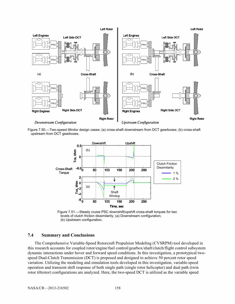
NASA/CR—2013-216502 158

Figure 7.50.—Two-speed tiltrotor design cases; (a) cross-shaft downstream from DCT gearboxes; (b) cross-shaft

upstream from DCT gearboxes.

Figure 7.51.—Steady cruise PSC downshift/upshift cross-shaft torques for two

levels of clutch friction dissimilarity; (a) Downstream configuration, (b) Upstream configuration.

7.4 Summary and Conclusions

The Comprehensive Variable-Speed Rotorcraft Propulsion Modeling (CVSRPM) tool developed in this research accounts for coupled rotor/engine/fuel control/gearbox/shaft/clutch/flight control subsystem dynamic interactions under hover and forward speed conditions. In this investigation, a prototypical two-speed Dual-Clutch Transmission (DCT) is proposed and designed to achieve 50 percent rotor speed variation. Utilizing the modeling and simulation tools developed in this investigation, variable-speed operation and transient shift response of both single path (single rotor helicopter) and dual path (twin rotor tiltrotor) configurations are analyzed. Here, the two-speed DCT is utilized as the variable speed

Cross-Shaft

FWU

FWU

FWU

FWU

Left Engines

Right Engines

Left Side DCT

Right Side DCT

Right Rotor

Left Rotor

Cross-Shaft

FWU

FWU

FWU

FWU

Left Engines

Right Engines

Left Side DCT

Right Side DCT

Right Rotor

Left Rotor

(a) (b)

Downstream Configuration Upstream Configuration

Cross-Shaft

FWU

FWU

FWU

FWU

Left Engines

Right Engines

Left Side DCT

Right Side DCT

Right Rotor

Left Rotor

Cross-Shaft

FWU

FWU

FWU

FWU

Left Engines

Right Engines

Left Side DCT

Right Side DCT

Right Rotor

Left Rotor

Cross-Shaft

FWU

FWU

FWU

FWU

Left Engines

Right Engines

Left Side DCT

Right Side DCT

Right Rotor

Left Rotor

Cross-Shaft

FWU

FWU

FWU

FWU

Left Engines

Right Engines

Left Side DCT

Right Side DCT

Right Rotor

Left Rotor

(a) (b)

Downstream Configuration Upstream Configuration

0 50 100 150 200 250-0.5

0

0.5

Tcs,

kN

m

0 50 100 150 200 250-6

-4

-2

0

2

Tcs,

kN

m

Time, sec

0 50 100 150 200 250-0.5

0

0.5

Tcs,

kN

m

0 50 100 150 200 250-6

-4

-2

0

2

Tcs,

kN

m

Time, sec

Clutch Friction Dissimilarity

1 %

2 %

(a)

Cross-Shaft Torque

Shaft Windup

(b)

Downshift Upshift

0 50 100 150 200 250-0.5

0

0.5

Tcs,

kN

m

0 50 100 150 200 250-6

-4

-2

0

2

Tcs,

kN

m

Time, sec

0 50 100 150 200 250-0.5

0

0.5

Tcs,

kN

m

0 50 100 150 200 250-6

-4

-2

0

2

Tcs,

kN

m

Time, sec

Clutch Friction Dissimilarity

1 %

2 %

(a)

Cross-Shaft Torque

Shaft Windup

(b)

Downshift Upshift

NASA/CR—2013-216502 159

elements in each drive-system. In the case of the tiltrotor configuration, the simulation parameters are based on the NASA LCTR-2 prototype operating in forward-flight airplane mode.

Here both Parallel Shifting Control (PSC) and Sequential Shifting Control (SSC) strategies are explored. In the PSC strategy, all branches of the multipath drive-system are shifted simultaneously, while under SSC, each branch is shifted in sequence to avoided shifting under full power conditions. The chief advantage of PSC is that gear ratio changes can made relatively rapidly without need to involve engine control during the shift. However, for large rotorcraft, the clutch power dissipation and thermal energy dissipation requirements may be prohibitive. In SSC, power to a specific branch is removed by reducing the setpoint speed of the associated engine thereby disengaging the overrunning clutch and enabling the transmission to shifted under minimal load. Thus, SSC significantly reduces clutch power dissipation and hence clutch heating. However the SSC strategy requires a multiengine/multi DCT drive system topology whereas the PSC strategy can be implemented on singe DCT and multi DCT architectures.

One main contribution of this investigation to the existing body of research is the evaluation of both the PSC and SSC shift strategies in a comprehensive rotorcraft drive system simulation model. In particular, this investigation builds upon previous variable-speed rotorcraft propulsion studies by 1) including a fully transient gas-turbine engine model, 2) including clutch stick-slip friction effects, 3) including driveshaft flexibility, and 4), incorporating a basic, fully trimmed, flight dynamics model to account for interactions with the flight and engine control systems.

In PSC, the engaging clutch pressure is linearly ramped up while the disengaging clutch pressure is simultaneously commanded to ramp down all while maintaining the engine setpoint speed of all engines. One of the key parameters in PSC is the clutch engagement/disengagement ramp rates. Under the PSC strategy, selecting clutch shift-rate results in a design tradeoff between transient engine surge margins and clutch frictional power dissipation.

In SSC, the sequential shifting provided smooth rotor speed changes while maintaining a constant forward speed setpoint and constant altitude. However, it was found that transient shocks produced by engine engagements and disengagements from their freewheeling clutches tended to produce brief excursions of the engine compressor surge limit. It was found that proper choice of dual-clutch transmission shift rate could minimize these excursions. In the sequential downshift case, it was found that slower shift rates tended to reduce the engine surge effects while the opposite trend was found for the pshift case.

Given the current trend toward tandem, tilt-rotor, multirotor, and co-axial rotor/pusher-prop configurations with numerous cross-shafting and multipath power flow arrangements (e.g., Boeing CH-47 and V-22, Sikorsky X-2 High Speed Lifter and Heavy Lift quad tiltrotor concepts), It is hoped that the analysis tools and results presented from the CVSRPM code will be utilized as a guide for investigating and evaluating new configurations and designs for fixed and variable speed rotorcraft under a variety of operating conditions.

NASA/CR—2013-216502 161

Appendix.—Comprehensive Variable Speed Rotorcraft Propulsion System Model

Figure A.1.—Two-speed rotorcraft driveline comprehensive simulation—main block.

NASA/CR—2013-216502 162

Figure A.2.—Two-speed tiltrotor driveline/engine/clutch/rotor/fuel control/flight dynamics block.

NASA/CR—2013-216502 163

Figure A.3.—2-DOF (altitude and forward speed) vehicle flight dynamics block.

Figure A.4.—Rigid rotor and blade pitch forward speed controller block.

Here note the gas turbine engine model, engine fuel control and dual clutch transmission model

simulation blocks are given in Sections 4.0 and 6.0, respectively.

NASA/CR—2013-216502 164

References 1. W. Johnson, G. K. Yamauchi and M.E. Watts “NASA Heavy Lift Rotorcraft Systems

Investigation.” NASA 213467, December 2005. 2. Z. Saribay, A. Lemanski, M. Elmoznino, “Pericyclic Non-Traction Continuously Variable Speed

Transmission (P-CVT): Rotorcraft Applications,” AHS International 62nd Annual Forum and Technology Display, Phoenix, AZ, May 9–11, 2006

3. J. Kish, “Vertical Lift Drive System Concept Studies Variable Speed/Two-Speed Transmissions,” NASA/CR—2002-211564, 2002.

4. Goi, T., Kawakami, K., Yamakawa, E., and Tanaka, H., “Variable Rotor Speed Transmission With High Speed Traction Drive,” Presented at the American Helicopter Society 55th Annual Forum, Montreal, Quebec, Canada. May 25-27, 1999.

5. Kluger, M.A., et al., “An Overview of Current CVT Mechanisms, Forces and Efficiencies,” SAE Technical Paper Series, 970687, 1997.

6. Davis, K., J. Frisk, and G. Jewett, “Pericyclic Differential,” Univ. of Connecticut, Dept. of Mechanical Eng., Sr. Design Project, April 2004.

7. Lemanski A.J, Monahan, T.J. ,”Non-Traction Pericyclic CVT’s,” 2004 International Continuously Variable and Hybrid Transmission Conference University of California, Davis, September 23-25, 2004.

8. White, G., Department of Mechanical Engineering, University of Technology, Loughborough Leics, England, “A Two-Path Variable Ratio Transmission With an Extended Range of Ratios,” The American Society of Mechanical Engineers, Paper No. 76-DET-37, 1976.

9. Parker, Richard J., Loewenthal, Stuart H., Fischer, George K., National Aeronautics and Space Administration, Lewis Research Center, “Design Studies of Continuously Variable Transmissions for Electric Vehicles,” Society of Automotive Engineers Congress, Detroit, Michigan, DOE/NASA/1044-12, NASA TM-81642, February 23-27, 1981.

10. Sauer, Georg, Institute of Agricultural Machinery, Technical University of Munich, Germany, “Continuously Variable Transmissions for Tractor Drive Line,” Report No 94-D-020, AGENG, Milano 1994.

11. J. Lin and R.G. Parker, “Mesh Stiffness Variation Instabilities in Two-Stage Gear Systems,” ASME Journal of Vibration and Acoustics, Vol. 124, 2002, pp. 68-76.

12. T.C. Lim and J. Li, “Dynamic Analysis of Multi-Mesh Counter-Shaft Transmission,” Journal of Sound and Vibration, Vol. 219, 1999, pp. 905-919.

13. R. Kasuba, and R. August, “Gear Mesh Stiffness and Load Sharing in Planetary Gearing,” ASME 4th Power Transmission Conference, ASME Paper 84-DET-229, 1984, Cambridge, MA.

14. Botman, M., 1976, “Epicyclic Gear Vibrations,” Journal of Engineering for Industry, 96: 811-815. 15. Botman, M., 1980, “Vibration Measurements on Planetary Gears of Aircraft Turbine Engines,”

AIAA Journal, 17: 351-357. 16. Schlecht, B., Schulze, T., and Hähnel, T., “Simulation of Torsional Vibrations, or Multibody-

System-Simulation – which Technique does the Wind Power Industry need for solving the Present-day Problems?,” In The Science of making Torque from Wind – Special Topic Conference, Delft University, April 2004.

17. R.C. Strawn and R. Biswas “Numerical Simulations of Helicopter Aerodynamics and Acoustics,” Journal of Computational and Applied Mathematics, 1996, Vol. 66 (1-2), pp. 471-483.

18. P.P. Friedmann and T.A. Millott, “Vibration Reduction in Rotorcraft Using Active Control – Comparison of Various Approaches,” Journal of Guidance Control and Dynamics, 1995, Vol. 18, No. 4, pp. 664-673.

19. R.E. Brown, “Rotor Wake Modeling for Flight Dynamic Simulation of Helicopters,” AIAA Journal, 2000, Vol. 38, No. 1 pp. 57-83.

20. G. Lehmann, “The Effect of Higher Harmonic Control (HHC) on a 4-Bladed Hingeless Model Rotor,” Vertica, 1985 Vol. 9, No. 3, pp. 273-284.

NASA/CR—2013-216502 165

21. Krothapalli, K.R., J.V.R. Prasad, D.A. Peters (2001) Helicopter Rotor Dynamic Inflow Modeling for Maneuvering Flight. Journal of the American Helicopter Society, 46: 129-139.

22. Morillo, J.A., and D.A. Peters (2002) Velocity Field Above A Rotor Disk by A New Dynamic Inflow Model. Journal of Aircraft, 39: 731-738.

23. Asokanthan, S. F. and Hwang, M. C., 1996, “Torsional Instabilities in a System Incorporating a Hooke’s Joint,” Journal of Vibration Acoustics, Vol. 118, pp. 386-374.

24. Chen, L. W. and Chen, H. K., 1995, “Whirl Speed and Stability of Rotating Shaft Subjected to End Loads,” AIAA Journal, Vol. 33, No. 9.

25. Iwatsubo, T. and Saigo, M., 1984, “Transverse Vibration of a Rotor System Driven by a Cardan Joint,” Journal of Sound and Vibration, Vol. 95, pp. 9-18.

26. Mazzei, A. J., Jr., Argento, A. and Scott, R. A., 1999, “Dynamic Stability of a Rotating Shaft Driven through a Universal Joint,” Journal of Sound and Vibration, Vol. 222, pp. 19-47.

27. DeSmidt, H. A., Wang, K. W. and Smith, E. C., 2002, “Coupled Torsion-Lateral Stability of A Shaft-Disk System Driven Through A Universal Joint,” ASME Journal of Applied Mechanics, Vol. 69, No. 3, pp. 261-273.

28. Kirk, R. G., Mondy, R. E. and Murphy, R. C., 1984, “Theory and Guidelines to Proper Coupling Design for Rotor Dynamics Considerations,” Journal of Vibration, Acoustics, Stress, and Reliability in Design, Vol. 106, pp. 129-138.

29. H. A. DeSmidt, K. W. Wang, and E. C. Smith, “Stability of a Segmented Supercritical Driveline with Non-Constant Velocity Couplings Subjected to Misalignment and Torque,” Journal of Sound and Vibration Vol. 277, No. 4-5, pp. 895-918, 2004.

30. H. A. DeSmidt, Robust-Adaptive Active Vibration Control of Alloy and Flexible Matrix Composite Rotorcraft Drivelines via Magnetic Bearings: Theory and Experiment, Ph.D. Thesis, The Pennsylvania State University, May 2005.

31. M.G. Ballin, “A High Fidelity Realtime Simulation of a Small Turboshaft Engine,” NASA TM 100991, July 1988.

32. C. Evans, D. Rees, and A. Borell, “Identification of aircraft gas turbine dynamics using frequency-domain techniques,” Control Engineering Practice, 2000, Vol. 8 No. 4 pp. 457–467.

33. K, Vazquez, “System applied strategies applied to aircraft gas turbine engines,” Control Engineering Practice, 2001, Vol. 9 No. 2, pp. 135–148.

34. O.M. Boaghe, S.A. Billings, L.M. Li and F.J. Lui, “Time and Frequency Domain Identification and Analysis of a Gas Turbine Engine,” Control Engineering Practice, 2002, Vol. 10, pp. 1347-1356.

35. A.S. Hopkins, G.C. Ruzicka and R.A. Ormiston, “Analytical Investigations of Coupled Rotorcraft/Engine/Drive Train Dynamics,” Proc. of the American Helicopter Society 2nd International Region Aero Mechanics Specialists’ Conf., Bridgeport, CT, Oct. 11-13, 1995.

36. L.C. Jaw and A.E. Bryson, Jr., “Modeling Rotor Dynamics With Rotor Speed Degree of Freedom for Drive Train Torsional Stability Analysis,” Proc. of 16th the European Rotorcraft Forum, Glasgow, Scotland, Sept. 21 1990.

37. K. Liu, M. Mittal, J.V.R. Prasad, C.J. Scholz, “A Study of Coupled Engine/Rotor Dynamic Behavior,” Proc. of the 51st Annual Forum of the American Helicopter Society, Fort Worth, TX, May. 9-11, 1995.

38. M. Roa, S.K. Biswas, B.P. Butz and D.G. Miller, “Dynamic Modeling and Feedback Control of a Side-by-Side Rotor Tandem Helicopter,” IEEE Paper Number TH0333-5/90/0000/0780, 1990, pp. 780-785.

39. Prouty, R. W., “Should We Consider Variable Rotor Speeds?” Vertiflite, Vol. 50, No. 4, 2004, pp. 24-27.

40. Maisel, M. D., Giulianetti, D., and Dugan, D., “The History of the XV-15 Tilt Rotor Research Aircraft: From Concept to Flight,” Tech. Rep. NASA/SP—2000-4517, 2000.

41. Johnson, W., Helicopter Theory, Princeton University Press, Princeton, NJ, 1980, pp. 393-397. 42. Han, D. and Smith, E. C., “Lagwise Loads Analysis of a Rotor Blade with an Embedded Chordwise

Absorber,” Journal of Aircraft, Vol. 46, No. 4, 2009, pp. 1280-1290.

NASA/CR—2013-216502 166

43. Hodges, D. H., and Dowell, E. H., “Nonlinear Equations of Motion for the Elastic Bending and Torsion of Twisted Non-Uniform Blades,” NASA TN D-7818, Dec. 1974.

44. Straub, F. K., Sangha, K. B., and Panda, B., “Advanced Finite Element Modeling of Rotor Blade Aeroelasticity,” Journal of the American Helicopter Society, Vol. 39, No. 2, 1994, pp. 56-68.

45. Zheng, Z. C., Ren, G., and Cheng, Y. M., “Aeroelastic Response of a Coupled Rotor/Fuselage System in Hovering and Forward Flight,” Archive of Applied Mechanics, Vol. 69, No. 1, 1999, pp. 68-82.

46. Peters, D. A. and HaQuang, N., “Dynamic Inflow for Practical Application,” Journal of the American Helicopter Society, Vol. 33, No. 4, 1988, pp. 64-68.

47. Owen, D. R. J. and Hinton, E., Finite Elements in Plasticity: Theory and Practice, Pineridge Press, Swansea, U.K., 1980, pp. 431-436.

48. Bagai, A., “Contribution to the Mathematical Modeling of Rotor Flow-Fields using a Pseudo-Implicit Free-Wake Analysis,” Ph.D. Thesis, University of Maryland, College Park, MD, 1995.

49. Leishman, J. G., Principles of Helicopter Aerodynamics, Cambridge Univ. Press, Cambridge, England, U.K., 2000.

50. Karem, A. E., Optimum Rotor Speed, United States Patent, 6007298, Dec. 28, 1999. 51. Wang, J. M. and Chopra, I., “Dynamics of Helicopter with Dissimilar Blades,” 47th Annual Forum

Proceedings of the American Helicopter Society, Phoenix, AZ, May 6-8 1991. 52. Roget, B. and Chopra, I., “Robust Individual Blade Control Algorithm for a Dissimilar Rotor,”

Journal of Guidance, Control, and Dynamics, Vol. 25, No. 5, 2002, pp. 915-923. 53. Stevens, P. W. and Smith, E. C., “Active Interrogation of Helicopter Rotor Faults using Trailing-

Edge Flap Actuation,” 57th Annual Forum Proceedings of the American Helicopter Society, Washington, DC, May 9-11 1991.

54. Han, D. and Smith, E.C, “Lagwise Resonance Crossing Analysis of a Variable Speed Rotor,” the 3rd International Basic Research Conference on Rotorcraft Technology, Nanjing, China, Oct. 14-16, 2009.

55. Zapfe, J. A. and Lesieutre, G. A., “Broadband Vibration Damping in Beams Using Distributed Viscoelastic Tuned Mass Absorbers,” Proceedings of the 37th AIAA/ASME/ASCE/AHS/ASC Structures, Structural Dynamics and Materials Conference, Salt Lake City, UT, April 1996.

56. Hébert, C. A. and Lesieutre, G. A., “Rotorcraft Blade Lag Damping Using Highly Distributed Tuned Vibration Absorbers,” Proceedings of the 39th AIAA/ASME/ASCE/AHS/ASC Structures, Structural Dynamics and Materials Conference, Long Beach, CA, April 1998.

57. Kang, H., Rotor Blade Damping Using Embedded Chordwise Absorbers, Ph.D. thesis, The Penn State University, 2001.

58. Kang, H., Smith, E. C., and Lesieutre, G. A., “The effects of Embedded Chordwise Absorbers on Blade Aeroelastic Stability,” Proceedings of the 43rd AIAA/ASME/ASCE/AHS/ASC Structures, Structural Dynamics and Materials Conference, Denver, CO, April 2002.

59. Kang, H., Smith, E. C., and Lesieutre, G. A., “Experimental and Analytical Study of Blade Lag Damping Augmentation Using Chordwise Absorbers,” Journal of Aircraft, Vol. 43, No. 1, 2006, pp. 194-200.

60. Petrie, J. S., Lesieutre, G. A., and Smith, E. C., “Helicopter Blade Lag Damping Using Embedded Fluid Elastic Chordwise Inertial Dampers,” Proceedings of the 45th AIAA/ASME/ASCE/AHS/ASC Structures, Structural Dynamics and Materials Conference, Palm Springs, CA, April 2004.

61. Petrie, J. S., Lesieutre, G. A., and Smith, E. C., “Design and Model Testing of Helicopter Rotor Blade Lag Fluid Elastic Embedded Chordwise Inertial Dampers,” 61st Annual Forum Proceedings of the American Helicopter Society, Grapevine, TX, Jun. 2005.

62. Petrie, J. S., “Helicopter Rotor Blade Lag Damping Using Fluid Elastic Embedded Chordwise Inertial Dampers,” Master Thesis, The Pennsylvania State University, University Park, PA, 2004, pp. 52-54.

NASA/CR—2013-216502 167

63. Jaw, L. C., Control of a Helicopter Engine in Low Altitude Flight, Ph.D. thesis, Stanford University, 2001.

64. Mazzei, A., and Scott, R. A. “Variable speed effects on stability of drivelines with universal joints.” Proceedings of the XXIV International Modal Analysis Conference, Saint Louis, MO, 2006.

65. Martin, G. H. Kinematics and Dynamics of Machines. McGraw Hill, 1969. 66. Nayfeh, A. H. and Mook. D. T. Nonlinear Oscillations. John Wiley & Sons, 1979. 67. Acree, Jr., C. W., and Johnson, Wayne. “Aeroelastic Stability of the LCTR2 Civil Tiltrotor.” AHS

Technical Specialists’ Meeting, Dallas, Texas, Oct., 2008. 68. Shokrieh, M. M., Hasani, A., and Lessard, L. B. “Shear Buckling of a Composite Drive Shaft

Under Torsion.” Composite Structures, 64(1):63-69, 2003. 69. Rao, S. S. Mechanical Vibrations. 4th ed. Pearson, 2004 70. Walsh, P. P., and Fletcher, P., 1998, Gas Turbine Performance, Blackwell Science, Oxford, Chap.

8, p. 468. 71. Smith, D. L., and Stammetti, V. A., 1990, “Sequential Linearization as an Approach to Real Time

Marine Gas Turbine Simulation,” J. Eng. Gas Turbines Power, 112, pp. 187–191. 72. Visser, P. J., Broomhead, M. J., and van der Vorst, J., 2001, “TERTS, A Generic Real-Time Gas

Turbine Simulation Environment,” ASME Paper No. 2001-GT-0446. 73. Stamatis, A., Mathioudakis, K., Ruiz, J., and Curnock, B., 2001, “Real Time Engine Model

Implementation for Adaptive Control & Performance Monitoring of Large Civil Turbofans,” ASME Paper No. 2001-GT-0362.

74. Camporeale, S. M., Fortunato, B., and Dumas, A., 1998, “Dynamic Modeling and Control of Regenerative Gas Turbines,” ASME Paper No. 98-GT-172

75. Agresti, M., Camporeale, S. M., and Fortunato, B., 2000, “An Object-Oriented Program for the Dynamic Simulation of Gas Turbines,” ASME Paper No. 2000-GT-42.

76. “Industrial Engine Performance-Natural Gas Fuel,” 1997, GE Report available from www.ge.com. 77. Spector, R. B., and Miller, A. A., 1983, “GE LM 2500 Aircraft-Derivative Gas Turbine System,”

General Electric Company Report GER 343. 78. Schobeiri, M. T., Attia, M., and Lippe, C., 1994, “GETRAN: A Generic Modularly Structured

Computer Code for Simulation of Dynamic Behavior of Aero- and Power Generation Gas Turbine Engines,” Trans. ASME: J. Eng. Gas Turbines Power, 116, pp. 483–494.

79. Kim, J. H., Song, T. W., Kim, T. S., and Ro, S. T., 2000, “Model Development and Simulation of Transient Behaviour of Heavy Duty Gas Turbines,” ASME Paper No. 2000-GT-0548.

80. Camporeale, S. M., Fortunato, B., and Mastrovito, M., 2006, “A Modular Code for Real Time Dynamics Simulation of Gas Turbines in Simulink,” Trans. ASME: J. Eng. Gas Turbines Power, 128, pp. 506-517.

81. Sekhon, R., Bassily, H., Wagner, J., and Gaddis, J., 2006, “Stationary Gas Turbines – A Real Time Dynamic Model with Experimental Validation,” Proc. of the American Control Conference, Minneapolis, Minnesota, USA, June 14-16, 2006.

82. Veres J. P., 2009, “Compressor Study to Meet Large Civil Tilt Rotor Engine Requirements,” AHS International, 65th Annual Forum & Technology Display, Grapevine, Texas, May 27–29, 2009.

83. Snyder, C.A., and Thurman, D.R., “Gas turbine characteristics for a Large Civil Tilt-Rotor (LCTR),” AHS International, 65th Annual Forum & Technology Display, Grapevine, Texas, May 27–29, 2009.

84. Benton, M., and Seireg, A., 1978, “Simulation of Resonances and Instability Conditions in Pinion-Gear Systems,” ASME J. Mech. Des., 100, pp. 26–30.

85. Kahraman, A., and Blankenship, G. W., 1996, “Interactions Between Commensurate Parametric and Forcing Excitations in a System with Clearance,” Journal of Sound and Vibration, 194, pp. 317–336.

86. Kahraman, A., and Blankenship, G. W., 1997, ‘‘Experiments on Nonlinear Dynamic Behavior of an Oscillator with Clearance and Periodically Time-Varying Parameters,’’ ASME J. Appl. Mech., 64, pp. 217–226.

NASA/CR—2013-216502 168

87. Blankenship, G. W., and Kahraman, A., 1995, “Steady State Forced Response of a Mechanical Oscillator with Combined Parametric Excitation and Clearance Type Nonlinearity,” Journal of Sound and Vibration, 185, pp. 743–765.

88. Kahraman, A., and Singh, R., 1991, “Interactions Between Time-varying Mesh Stiffness and Clearance Nonlinearities in a Geared System,” Journal of Sound and Vibration, 146, pp. 135–156.

89. Lin, J., and Parker, R. G., 2002, ‘‘Planetary Gear Parametric Instability Caused by Mesh Stiffness Variation,” Journal of Sound and Vibration, 249, pp. 129–145.

90. J. Lin, R.G. Parker, “Mesh stiffness vibration instabilities in two-stage gear systems,” Journal of Vibration and Acoustics, 124 (2002) 68–76.

91. Benton, M., and Seireg, A., 1981, “Factors Influencing Instability and Resonances in Geared Systems,” ASME J. Mech. Des., 103, pp. 372–378.

92. Amabili, M., and Rivola, A., 1997, “Dynamic Analysis of Spur Gear Pairs: Steady-State Response and Stability of the SDOF Model With Time-Varying Meshing Damping,” Mech. Syst. Signal Process, 11, pp. 375–390.

93. Kahraman, A., and Blankenship, G. W., 1999, “Effect of Involute Contact Ratio on Spur Gear Dynamics,” ASME J. Mech. Des., 121, pp. 112–118.

94. M. Vaishya and R. Singh, “Analysis of Periodically Varying Gear Mesh Systems with Coulomb Friction Using Floquet Theory,” Journal of Sound and Vibration, 243(3) (2001) 525-545.

95. Kahraman, J. Lim, and H. Ding, “A Dynamic Model of a Spur Gear Pair with Friction,” Proc. 12th IFToMM World Congress, Besançon (France), June18-21, 2007.

96. H. Vinayak, R. Singh, C. Padmanabhan, “Linear dynamic analysis of multi-mesh transmissions containing external rigid gears,” Journal of Sound and Vibration, 185, 1995, 1–32.

97. S. V. Neriya, R. B. Bhat, T. S. Sankar, Effect of coupled torsional-flexural vibration of a geared shaft system on the dynamic tooth load, The Shock and Vibration Bulletin, 54, 1984, 67–75.

98. S. Lee, J. W. Ha, and D. H. Choi, “Coupled lateral and torsional vibration characteristics of a speed increasing geared rotor-bearing system” Journal of Sound and Vibration, 263, 2003, 725-542.

99. S. H. Choi, J. Glienicke, D. C. Han, K. Urlichs, “Dynamic gear load due to coupled lateral, torsional and axial vibrations in a helical geared system,” Journal of Vibration and Acoustics, 121, 1999, 141–148.

100. M. Kubur, A. Kahraman, D. Zini, K. Kienzle, Dynamic analysis of a multi-shaft helical gear transmission by finite elements: model and experiment, Journal of Vibration and Acoustics, 126, 2004, 398–406.

101. S. Lee and J. W. Ha, “Prediction of maximum unbalance responses of a gear-coupled two-shaft rotor-bearing system,” Journal of Sound and Vibration, 283, 2005, 507-523.

102. J. Wang and I. Howard, “The torsional stiffness of involute spur gears,” Journal of Mechanical Engineering Science, 218 part C (2004) 131–142.

103. Y. Kuznetsov, Elements of Applied Bifurcation Theory, Second Edition, Springer-Verlag 1998, New York, pp. 478-484.

104. Acree, C.W., Yeo, H., and Sinsay, J.D., “Performance Optimization of the NASA Large Civil Tiltrotor,” International Powered Lift Conference, London, UK, Jul. 22-24, 2008.

105. Bossler, R.B., “Vertical Lift Drive System Concept Studies,” NASA/CR—2002-211563, Army Research Laboratory Contractor Report ARL-CR-0496, Grant NAG3-2570, Jun. 2002.

106. Ai, X., Mohr, T., and Anderson, S., “An Electro-Mechanical Infinitely Variable Speed Transmission,” SAE 2004 World Congress, Detroit, MI, Mar. 8-11, 2004.

107. Saribay, Z., Smith, E., Lemanski, A., Bill, R., Wang, K.W., and Rao, S., “Compact Pericyclic Continuously Variable Speed Transmission Systems: Design Features and High-Reduction Variable Speed Case Studies,” American Helicopter Society 63nd Annual Forum, Virginia Beach, VA, May 1-3, 2007.

108. Stevens, M.A., Handschuh, R.F., and Lewicki, D.G., “Variable/Multispeed Rotorcraft Drive System Concepts,” NASA/TM—2009-215456, Army Research Laboratory Report ARL-TR-4758, Mar. 2009.

NASA/CR—2013-216502 169

109. Hong, K., Yang, K., and Lee, K., “An Object-Oriented Modular Simulation Model for Integrated Gasoline Engine and Automatic Transmission Control,” SAE transactions, Vol. 108, No. 6, Part 1, pp. 1349-1357, 1999.

110. Haj-Fraj, A., and Pfeiffer, F., “Optimization of Gear Shift Operations in Automatic Transmissions,” Proceedings of the 6th International Workshop on Advanced Motion Control, Nagoya, Japan, pp. 469-473, 2000.

111. Jung, G., Cho, B., and Lee, K., “Dynamic Analysis and Closed-Loop Shifting Control of EF-Automatic Transmission with Proportional Control Solenoid Valves,” FISITA World Automotive Congress, Seoul, Korea, pp. 12–15, 2000.

112. Gong, J., Zhao, D., Chen, Y., and Chen, N., “Study on Shift Schedule Saving Energy of Automatic Transmission of Ground Vehicles,” Journal of Zhejiang University-Science A, Vol. 5, No. 7, pp. 878-883, 2004.

113. Watechagit, S., “Modeling and Estimation for Stepped Automatic Transmission with Clutch-to-Clutch Shift Technology,” PhD Dissertation, The Ohio State University, Department of Mechanical Engineering, 2004.

114. Kim, D., Peng, H., Bai, S., and Maguire, J., “Control of Integrated Powertrain with Electronic Throttle and Automatic Transmission,” IEEE Transactions on Control Systems Technology, Vol. 15, No. 3, pp. 474, 2007.

115. Lu, X., Xu, X., and Liu, Y., “Simulation of Gear-Shift Algorithm for Automatic Transmission Based on MATLAB,” Proceedings of the 2009 World Research Institute World Congress on Software Engineering, pp. 476-480, May 19-21, 2009.

116. Lin, C., Peng, H., Grizzle, J., and Kang, J., “Power Management Strategy for a Parallel Hybrid Electric Truck,” IEEE Transactions on Control Systems Technology, Vol. 11, No. 6, pp. 839-849, 2003.

117. Yamamoto, M., Wakahara, T., Okahara, H., and Oshita, H., “Hydraulic System, Shift and Lock-Up Clutch Controls Developed for a Large Torque Capacity CVT,” International Continuously Variable and Hybrid Transmission Congress, Paper No. 04CVT-07, 2004.

118. Lu, Z, “Acceleration Simulation of a Vehicle with a Continuously Variable Power Split Transmission,” Master's Thesis, West Virginia University, Department of Mechanical Engineering, 1998.

119. Wicke, V., Brace, C., and Vaughan, N., “The Potential for Simulation of Drivability of CVT Vehicles,” SAE Transactions, Vol. 109, No. 6, pp. 1205-1210, 2000.

120. Klaassen, T., et al., “Modeling and Simulation of an Electro-Mechanically Actuated Pushbelt Type Continuously Variable Transmission,” Mechatronic Systems 2004: A Proceedings Volume From the 3rd IFAC Symposium, Sydney, Australia, Sep. 2004.

121. Togai, K., and Koso, M., “Dynamic Scheduling Control for Engine and Gearshifts: Consolidation of Fuel-Economy Optimization and Reserve Power,” Mitsubishi Motors Technical Review No. 18, 2006.

122. Anthony, J., Moskwa, J., and Danielson, E., “Powertrain Simulation of the M1A1 Abrams Using Modular Model Components,” SAE International Congress & Exposition, Detroit, MI, Feb. 1998.

123. Assanis, D., et al., “Validation and Use of SIMULINK Integrated, High Fidelity, Engine-in-Vehicle Simulation of the International Class VI Truck,” SAE Transactions, Vol. 109, No. 3, pp. 384-399, 2000.

124. Fathy, H., Ahlawat, R., and Stein, J., “Proper Powertrain Modeling for Engine-in-the-Loop Simulation,” Proceedings of the 2005 ASME International Mechanical Engineering Congress and Exposition, Orlando, FL, 2005.

125. Yi, J., Wang, X., Hu, Y., and Li, C., “Fuzzy Control and Simulation on Automatic Transmission of Tracked Vehicle in Complicated Driving Conditions,” 2006 IEEE International Conference on Vehicular Electronics and Safety, pp. 259-64, 2007.

NASA/CR—2013-216502 170

126. Nedungadi, A., Pozolo, M., and Mimnagh, M., “A General Purpose Vehicle Powertrain Modeling and Simulation Software-VPSET,” 2008 World Automation Congress Conference, Waikoloa, HI, 2008.

127. Lewicki, D.G., DeSmidt, H.A., Smith, E.C., and Bauman, S.W., “Two-Speed Gearbox Dynamic Simulation Predictions and Test Validation,” Proc. 66th American Helicopter Society Annual Forum, Phoenix, AZ., May 2010.

128. Lacraru, L.M. and Bouazza-Marouf, K., “Friction compensation of an actively restrained clutch for path tracking,” Proc. of the IMechE, Part I: J. of Sys. and Ctrl. Engr. Vol. 220, No. 5, pp. 381-393, 2006.

129. Crowther, A., Zhang, N., Liu, D.K., Jeyakumaran, J.K., “Analysis and Simulation of Clutch Engagement Judder and Stick-Slip in Automotive Powertrain Systems, Proc. Instn Mech. Engrs, Part D: J. Automobile Engineering, 218, pp. 1427-1446, 2004.

130. Liu, Y., Qin, D., Jiang, H. and Zhang, Y., “A Systematic Model for Dynamics and Control of Dual Clutch Transmissions,” Journal of Mechanical Design, ASME Trans. 131 (2009) 061012.

131. Sturgeon, W.R., “A Mathematical Model of the CH-53 Helicopter,” NASA TM–81238, 1980. 132. Litt, J.S., Edwards, J.M., and DeCastro, J.A., “A Sequential Shifting Algorithm for Variable Rotor

Speed Control,” NASA/TM—2007-214842 (2007)