COMPOSITE CLOCKS WITH 3-STATE MODELS · 39th Annual Precise Time and Time Interval (PTTI) Meeting ....

39th Annual Precise Time and Time Interval (PTTI) Meeting

COMPOSITE CLOCKS WITH 3-STATE MODELS

James R. Wright Analytical Graphics, Inc.

220 Valley Creek Blvd., Exton, PA 19341, USA E-mail: [email protected]

Abstract

Previous analyses of composite clocks have been presented with 2-state clock models for random clock phase and frequency deviations. But Kalman filter estimate errors due to 3-state clock frequency-drift deviations have not been previously presented. I have employed the 3-state Zucca-Tavella clock model to simulate an ensemble of four 3-state clocks. I have found a dominant common component for 3-state clock Kalman filter phase errors with the curvature of a nonlinear low-order polynomial that does not exist for 2-state clocks. Cesium clocks are free of frequency-drift, but rubidium and hydrogen-maser clocks have significant frequency drift. Use of the 3-state clock model, and an understanding of its true and estimated behavior, will facilitate operation of the associated composite clock.

I. INTRODUCTION

GPS Time is created by processing GPS pseudo-range measurements with the operational GPS Kalman filter. Brown [2] refers to the object created by the Kalman filter as the GPS Composite Clock, and to GPS Time as the Implicit Ensemble Mean phase of the GPS Composite Clock. The fundamental goal by the USAF and the USNO is to control GPS Time to within a specified bound of UTC/TAI. I present here a quantitative analysis of a simulated GPS Composite Clock, derived from detailed simulations and associated graphics. GPS clock diffusion coefficient values used here were selected to enable a characterization of 3-state clocks that illuminate the effects of frequency-drift. Diffusion coefficient values used for each of the four clocks S1, S2, N1, and N2 are presented in several of the initial figures. S1 and S2 refer to ground station clocks. N1 and N2 refer to NAVSTAR clocks. My interest in the GPS Composite Clock derives from my interest in performing real-time orbit determination1 for GPS NAVSTAR spacecraft from ground receiver pseudo-range measurements. The estimation of NAVSTAR orbits would be incomplete without the simultaneous estimation of GPS clock parameters. I use simulated GPS clock phase, frequency, and frequency-drift deviations, and simulated GPS pseudo-range measurements, to study Kalman filter estimation errors. I am indebted to Charles Greenhall (JPL) for encouragement and help in this work. II. COMPLETE ESTIMATION AND CONTROL PROBLEM The USNO operates two UTC/TAI master clocks, each of which provides access to an estimate of UTC/TAI in real-time (1 pps). One of these clocks is maintained at the USNO, and the other is maintained at Shriever Air

371

Report Documentation Page Form ApprovedOMB No. 0704-0188

Public reporting burden for the collection of information is estimated to average 1 hour per response, including the time for reviewing instructions, searching existing data sources, gathering andmaintaining the data needed, and completing and reviewing the collection of information. Send comments regarding this burden estimate or any other aspect of this collection of information,including suggestions for reducing this burden, to Washington Headquarters Services, Directorate for Information Operations and Reports, 1215 Jefferson Davis Highway, Suite 1204, ArlingtonVA 22202-4302. Respondents should be aware that notwithstanding any other provision of law, no person shall be subject to a penalty for failing to comply with a collection of information if itdoes not display a currently valid OMB control number.

1. REPORT DATE NOV 2007 2. REPORT TYPE

3. DATES COVERED 00-00-2007 to 00-00-2007

4. TITLE AND SUBTITLE Composite Clocks with 3-State Models

5a. CONTRACT NUMBER

5b. GRANT NUMBER

5c. PROGRAM ELEMENT NUMBER

6. AUTHOR(S) 5d. PROJECT NUMBER

5e. TASK NUMBER

5f. WORK UNIT NUMBER

7. PERFORMING ORGANIZATION NAME(S) AND ADDRESS(ES) Analytical Graphics, Inc,220 Valley Creek Blvd,Exton,PA,19341

8. PERFORMING ORGANIZATIONREPORT NUMBER

9. SPONSORING/MONITORING AGENCY NAME(S) AND ADDRESS(ES) 10. SPONSOR/MONITOR’S ACRONYM(S)

11. SPONSOR/MONITOR’S REPORT NUMBER(S)

12. DISTRIBUTION/AVAILABILITY STATEMENT Approved for public release; distribution unlimited

13. SUPPLEMENTARY NOTES 39th Annual Precise Time and Time Interval (PTTI) Meeting, 26-29 Nov 2007, Long Beach, CA

14. ABSTRACT Previous analyses of composite clocks have been presented with 2-state clock models for random clockphase and frequency deviations. But Kalman filter estimate errors due to 3-state clock frequency-driftdeviations have not been previously presented. I have employed the 3-state Zucca-Tavella clock model tosimulate an ensemble of four 3-state clocks. I have found a dominant common component for 3-state clockKalman filter phase errors with the curvature of a nonlinear low-order polynomial that does not exist for2-state clocks. Cesium clocks are free of frequency-drift, but rubidium and hydrogen-maser clocks havesignificant frequency drift. Use of the 3-state clock model, and an understanding of its true and estimatedbehavior, will facilitate operation of the associated composite clock.

15. SUBJECT TERMS

16. SECURITY CLASSIFICATION OF: 17. LIMITATION OF ABSTRACT Same as

Report (SAR)

18. NUMBEROF PAGES

20

19a. NAME OFRESPONSIBLE PERSON

a. REPORT unclassified

b. ABSTRACT unclassified

c. THIS PAGE unclassified

Standard Form 298 (Rev. 8-98) Prescribed by ANSI Std Z39-18


Force Base in Colorado Springs. This enables the USNO to compare UTC/TAI to the phase of each GPS orbital NAVSTAR clock via GPS pseudo-range measurements, by embedding a UTC/TAI master clock in a USNO GPS ground receiver. Each GPS clock is a member of (internal to) the GPS ensemble of clocks, but the USNO master clock is external to the GPS ensemble of clocks. Because of this, the difference between UTC/TAI and the phase of each NAVSTAR GPS clock is observable. This difference can be (and is) estimated and quantified. The RMS (Root Mean Square) on these differences quantifies the difference between UTC/TAI and GPS Time. Inspection of the differences between UTC/TAI and the phase of each NAVSTAR GPS clock enables the USNO to identify GPS clocks that require particular frequency-rate control corrections. Use of this knowledge enables the USAF to adjust frequency rates of selected GPS clocks. Currently, the USAF uses an automated bang-bang controller3 on frequency-rate. III. STOCHASTIC CLOCK PHYSICS The most significant stochastic clock physics are understood in terms of Wiener processes and their integrals. Clock physics are characterized by particular values of clock-dependent diffusion coefficients, and are conveniently studied with aid of a relevant clock model that relates diffusion coefficient values to their underlying Wiener processes. For my presentation here, I have selected “The Clock Model and Its Relationship with the Allan and Related Variances” presented as an IEEE paper by Zucca and Tavella [18] in 2005. Except for FM flicker noise, this model captures the most significant physics for all GPS clocks. I simulate and validate GPS pseudo-range measurements using simulated phase deviations, simulated frequency deviations, and simulated frequency-drift deviations according to Zucca and Tavella. Figure 1 presents an ensemble of simulated random 3-state clock phase deviations, overlaid with independently calculated 3σ boundaries.

300000 800000 1300000 1800000tau(s)

-5.00e-6

-3.00e-6

-1.00e-6

1.00e-6

3.00e-6

Clock Phase Simulation ValidationZucca-Tavella

σ1 = 3.0e-12 √sσ2 = 5.0e-16 1/√sσ3 = 1.0e-21 1/√s^3

Clock Phase Deviation (s)

+3σ

-3σDIFFUSION COEFFICIENT VALUES

Figure 1. 3-State clock phase simulations.

372


IV. GRAPHICS FOR CASE 13 True deviations for 3-state clocks were simulated for Case 13 and were used to construct GPS pseudo-range measurements. The measurements were processed by the Kalman filter (KF1) described below with initial state estimate clock deviation errors. The simulated (true) clock phase deviations and estimated clock phase deviations are presented in Figure 2. Usually, one expects the phase estimates to lie close to the truth. This is not the case here, because the clock phase deviations are not observable from the GPS pseudo-range measurements. Nonetheless, estimated clock phase deviations are created by KF1. The simulated (true) clock frequency deviations and estimated clock frequency deviations are presented in Figure 3. Inspection of Figure 3 helps to explain the divergence with time between true clock phase deviations and estimated clock phase deviations presented in Figure 2.

100000 300000 500000 700000time(s)

-8.000e-7

-6.000e-7

-4.000e-7

-2.000e-7

0.000e0

2.000e-7

Simulated & Estimated Phase Deviates (s)Case 13

simulated

estimated

S1

S2

S2

N1

N1

N2

N2

KF1 initialization errors

← 8 days →

Same Diffusion Coefficient Values S1, S2, N1, N2sig 1 = 3e-12 √s sig 2 = 5e-16 1/√s sig 3 = 1e-21 1/s^3/2

PRN seedsS1: 120000000S2: 150000000N1: 180000000N2: 210000000

3-state clocksS1

Figure 2. Simulated & estimated phase deviates.

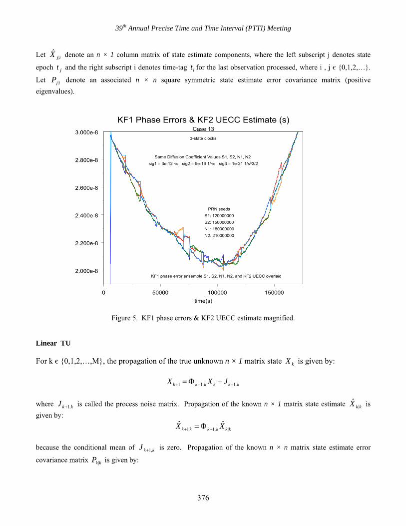
The estimated clock deviations were subtracted from the true (simulated) clock deviations to enable inspection of KF1 estimation errors. Estimation errors for the four clocks in phase, frequency, and frequency drift are presented in Figures 4, 5, 6, and 7. Figure 4 is deceptive in that one might be led to believe the KF1 phase errors are smooth with time. Figure 5 magnifies an interval of Figure 4 to demonstrate that KF1 phase errors are not smooth for 3-state clocks. Except for initial KF1 phase errors, Figure 4 demonstrates that most of the phase estimation errors for the four clocks S1, S2, N1, and N2 are similar. These similar phase errors are the unobservable components of KF1 estimation error common to each clock. Figure 5 enables identification of KF1 estimation errors that are independent for each clock with perturbations. These perturbations are the observable components of KF1 estimation errors. Continued processing of GPS pseudo-range measurements will reduce the variances on the observable components.

373


The common unobservable phase component for the four clocks S1, S2, N1, and N2 has been estimated with a second Kalman filter (KF2). This common phase component was subtracted from the KF1 phase error for S1 to enable identification of the observable component in KF1 phase error for S1. The latter is presented in Figure 8. V. KALMAN FILTER I present my approach for the optimal sequential estimation of clock deviation states and their error covariance functions. Sequential state estimates are generated recursively from two multidimensional stochastic update functions, the time update (TU), and the measurement update (MU). The TU moves the state estimate and covariance forward with time, accumulating integrals of random clock deviation process noise in the covariance. The MU is performed at a fixed measurement time where the state estimate and covariance are corrected with new observation information. The sequential estimation of GPS clock deviations requires the development of a linear TU and nonlinear MU. The nonlinear MU must be linearized locally to enable application of the linear Kalman MU. Kalman’s MU [9] derives from Sherman's Theorem [12,13,10]; Sherman's Theorem derives from Anderson's Theorem [1]; and Anderson's Theorem derives from the Brunn-Minkowki Inequality Theorem [14,5]. The theoretical foundation for my linearized MU derives from these theorems.

100000 300000 500000 700000time(s)

-2.000e-12

-1.500e-12

-1.000e-12

-5.000e-13

0.000e0

5.000e-13

1.000e-12

Simulated & Estimated Frequency Deviates (s/s)Case 13

simulated

estimated

N2

N1S1

S2

N2N1S1

S2

KF1 initialization errors

Same Diffusion Coefficient Values S1, S2, N1, N2sig1 = 3e-12 √s sig2 = 5e-16 1/√s sig3 = 1e-21 1/s^3/2

PRN seedsS1: 120000000S2: 150000000N1: 180000000N2: 210000000

3-state clocks

Figure 3. Simulated & estimated frequency deviates.

374


VA. INITIAL CONDITIONS Initialization of all sequential estimators requires the use of an initial state estimate column matrix and an

initial state estimate error covariance matrix for time t . 0|0X̂

0|0P 0

VB. LINEAR TU AND LINEAR MU Derivation and calculation for the discrete-time Kalman filter, linear in both TU and MU, is best presented by Meditch [10], Chapter 5.

100000 300000 500000 700000time(s)

-2.000e-7

0.000e0

2.000e-7

4.000e-7

KF1 Phase Errors & KF2 UECC Estimate (s)Case 13

KF1 phase error ensemble S1, S2, N1, N2, and KF2 UECC overlaid


PRN seedsS1: 120000000S2: 150000000N1: 180000000N2: 210000000

KF1 range sig = 1 cmtime granularity = 30 s, when visible

3-state clocks

Figure 4. KF1 phase errors & KF2 UECC estimate.

VC. LINEAR TU AND NONLINEAR MU The simultaneous sequential estimation of GPS clock phase and frequency deviation parameters can be studied with the development of a linear TU and nonlinear MU for the clock state estimate subset. This is useful to study clock parameter estimation, as demonstrated in Section VIII.

375


Let denote an n × 1 column matrix of state estimate components, where the left subscript j denotes state

epoch and the right subscript i denotes time-tag for the last observation processed, where i , j є {0,1,2,…}.

Let denote an associated n × n square symmetric state estimate error covariance matrix (positive eigenvalues).

ijX |ˆ

jt

ijP |

it

0 50000 100000 150000time(s)

2.000e-8

2.200e-8

2.400e-8

2.600e-8

2.800e-8

3.000e-8

KF1 Phase Errors & KF2 UECC Estimate (s)Case 13

3-state clocks

KF1 phase error ensemble S1, S2, N1, N2, and KF2 UECC overlaid

Same Diffusion Coefficient Values S1, S2, N1, N2sig1 = 3e-12 √s sig2 = 5e-16 1/√s sig3 = 1e-21 1/s^3/2

PRN seedsS1: 120000000S2: 150000000N1: 180000000N2: 210000000

Figure 5. KF1 phase errors & KF2 UECC estimate magnified.

Linear TU For k є {0,1,2,…,M}, the propagation of the true unknown n × 1 matrix state is given by: kX

1 1,k k k k kX X+ + +1,kJ= Φ +

where is called the process noise matrix. Propagation of the known n × 1 matrix state estimate is given by:

kkJ ,1+ kkX |ˆ

1| 1, |ˆ ˆ

k k k k k kX X+ += Φ

because the conditional mean of is zero. Propagation of the known n × n matrix state estimate error

covariance matrix is given by: kkJ ,1+

kkP |

376


1| 1, | 1, 1,T

k k k k k k k k k kP P+ + += Φ Φ +Q +

where the n × n matrix is called the process noise covariance matrix4 . kkQ |1+

Nonlinear MU Calculate the n × 1 matrix filter gain : 1+kK

1

1 1| 1 1 1| 1 1T T

k k k k k k k k kK P H H P H R−

+ + + + + + +⎡ ⎤= +⎣ ⎦

The filter measurement update state estimate n × 1 matrix , due to the observation , is calculated with: 1|1ˆ

++ kkX 1+ky

( )1| 1 1| 1 1 1|ˆ ˆ ˆ

k k k k k k k kX X K y y X+ + + + + +⎡ ⎤= + −⎣ ⎦

where is the scalar variance on the observation residual1+kR ( )kkk Xyy |11ˆ

++ − , and ( )kkXy |1ˆ

+ is a nonlinear

function of . Define the error in : kk |1+X̂ 1|1ˆ

++ kkXΔ X̂ 1|1 ++ kk

1| 1 1 1| 1ˆ ˆ

k k k k kX X X+ + + +Δ = − +

100000 700000300000 500000time(s)

KF s)

N1, N2 overlaid

PRN seedsS1: 120000000S2: 150000000N1: 180000000N2: 210000000

Same Diffusion sig 1 = 3e-12 √s

kP

1 Frequency Errors (s/Case 13

KF1 frequency error ensemble S1, S2,

Coefficient Values S1, S2, N1, N2sig 2 = 5e-16 1/√s sig 3 = 1e-21 1/s^3/2


3-state clocks

-1.000e-12

-5.000e-13

0.000e0

5.000e-13

1.000e-12

1.500e-12

Figure 6. KF1 frequency Errors.

Define the n × n state estimate error covariance matrix with: 1|1 ++ k

377


( )( ){ }1| 1 1| 1 1| 1ˆ ˆ T

k k k k k kP E X X+ + + + + += Δ Δ

Bucy and Joseph [3] (page 141) recommend that be calculated with: 1|1 ++ kkP

T

1| 1 1|k k k kP P+ + += − where:

11| 1 1 1 1|

Tk k k k k k kT P H R H P−+ + + + += %

has symmetry, and:

1 1 1| 1T

k k k k k 1kR H P H R+ + + + += +% Calculation of by the last three equations is numerically symmetric. They reduce to the form given by Kalman:

1|1 ++ kkP

[ ]1| 1 1 1 1|k k k k k kP I K H P+ + + + += −

which is not numerically symmetric.

100000 300000 500000 700000time(s)

-1.000e-17

-5.000e-18

0.000e0

5.000e-18

1.000e-17

KF1 Drift Errors (s/s^2)Case 13

KF1 frequency-drift error ensemble S1, S2, N1, N2 overlaid

PRN seedsS1: 120000000S2: 150000000N1: 180000000N2: 210000000


3-state clocks


Figure 7. KF1 drift errors.

VD. NONLINEAR TU AND NONLINEAR MU Refer to Subsection Nonlinear MU of Section VC for the nonlinear MU.

378


Nonlinear TU The nonlinear TU always spans a non-empty time interval and requires the use of a numerical state estimate integrator xϕ . Given an initial time , a final time , and a force model 0t ft ( )( )ttXu ,ˆ , then xϕ propagates the

state estimate from to t using forces ( )0ˆ tX 0t f ( )( )tX̂ t ,u to get ( )ftX̂ . That is:

( ) ( ) ( )( ){ }0 0 0ˆ ˆ ˆ; , , , ,f x f fX t t X t t u X t tφ τ τ= ≤τ ≤

This can be shortened to write:

( ) ( ){ }0 0ˆ ˆ; ,f x fX t t X tφ= t

where the use of force function ( )( )ttX ,ˆu x is tacitly implied. Thus, ϕ is a column matrix with n elements:

1

2

3

x

x

z x

xn

φφ

φ φ

φ

⎡ ⎤⎢ ⎥⎢ ⎥⎢ ⎥=⎢ ⎥⎢ ⎥⎢ ⎥⎣ ⎦

M

VE. KALMAN FILTER ADVANTAGE Severe computational problems are incurred in any attempt to estimate unobservable states using iterated batch least-squares methods or iterated maximum likelihood methods for navigation, because state-sized inversions of singular matrices are always required. Here, the Kalman filter is distinguished in that estimates of unobservable states can be created and used without matrix inversion problems, because the Kalman filter MU is free of state-sized matrix inversions. By design, one typically estimates observable states. But the Kalman filter enables one to create unobservable states. The USAF chose to create unobservable GPS clock parameter states for construction of GPS Time. VI. KALMAN FILTERS KF1 AND KF2 I have simulated GPS pseudo-range measurements for two GPS ground-station clocks S1 and S2, and for two GPS NAVSTAR clocks N1 and N2. Here, I set simulated measurement time granularity to 30 s for the set of all visible link intervals. Visible and non-visible intervals are clearly evident in Figure 8. I set the scalar root-variance R for both measurement simulations and Kalman filter KF1 to 1=R cm. Typically 1=R m for GPS pseudo-range, but when carrier-phase measurements are processed simultaneously with pseudo-range, the root-variance is reduced by two orders of magnitude. So the use of 1=R cm enables me to quantify lower performance bounds for the simultaneous processing of both measurement types. VIA. CREATE GPS CLOCK ENSEMBLE Typically, one processes measurements with a Kalman filter to derive sequential estimates of a multidimensional observable state. Instead, here I imitate the GPS operational procedure and process simulated GPS pseudo-range measurements with KF1 to create a sequence of unobservable multidimensional clock state estimates. Clock state

379


components are unobservable from GPS pseudo-range measurements. See Figure 2 for an example of an ensemble of estimated unobservable clock phase deviation state components created by KF1. Sherman's Theorem GPS Time, the unobservable GPS clock-ensemble mean phase, is created by the use of Sherman's Theorem [10,15] in the USAF Kalman filter measurement update algorithm on GPS range measurements. Satisfaction of Sherman's Theorem guarantees that the mean-squared state estimate error on each observable state estimate component is minimized. But the mean-squared state estimate error on each unobservable state estimate component is not reduced. Thus, the unobservable clock phase deviation state estimate component common to every GPS clock is isolated by application of Sherman's Theorem. An ensemble of unobservable state estimate components is, thus, created by Sherman's Theorem – see Figure 2 for an example. VIB. INITIAL CONDITION ERRORS A significant result emerges due to the modeling of Kalman filter (KF1) initial condition errors in phase, frequency, and frequency-drift. Initial estimated clock phase deviations are significantly displaced by the KF1 initial condition errors in phase. As time evolves, estimated clock phase deviation magnitudes diverge continuously and increasingly when referred to true (simulated) phase deviations, and this is due to filter initial condition errors in frequency and frequency drift. See Figures 3 and 2 for an example. VIC. PARTITION OF KF1 ESTIMATION ERRORS Subtract estimated clock deviations from simulated (true) clock deviations to define and quantify Kalman filter (KF1) estimation errors. Adopt Brown’s additive partition of KF1 estimation errors into two components. I refer to the first component as the Unobservable Error Common to each Clock (UECC), and to the second component as the Observable5 Error Independent for each Clock (OEIC). Initially, the variances on the UECC and OEIC are identical. On processing the first GPS pseudo-range measurements with KF1, the variances on both fall quickly. But with continued measurement processing, the variances on the UECC increase without bound, while the variances on the OEIC approach zero asymptotically. For simulated GPS pseudo-range data, I create an optimal sequential estimate of the UECC by application of a second Kalman filter KF2 to pseudo-measurements defined by the phase components of KF1 estimation errors. Since there is no physical process noise6 on the UECC, an estimate of the UECC can also be achieved using a batch least-squares estimation algorithm on the phase components of KF1 estimation errors – demonstrated previously by Greenhall [6,7]. VID. UNOBSERVABLE ERROR COMMON TO EACH CLOCK There are at least four techniques to estimate the UECC when simulating GPS pseudo-range data. First, one could take the sample mean of KF1 estimation errors across the clock ensemble at each time and form a sample variance about the mean; this would yield a sequential sampling procedure, but where each mean and variance is sequentially unconnected. Second, one can employ Ken Brown's Implicit Ensemble Mean (IEM) and covariance; this is a batch procedure requiring an inversion of the KF1 covariance matrix followed by a second matrix inversion of the modified covariance matrix inverse; this is not a sequential procedure. Third, one can adopt the new procedure by Charles Greenhall [7] wherein KF1 phase estimation errors are treated as pseudo-measurements, and are processed by a batch least-squares estimator to obtain optimal batch estimates and covariance matrices for the UECC. Fourth, one can treat the KF1 phase estimation errors as pseudo-

380


measurements, invoke a second Kalman filter (KF2), and process these phase pseudo-measurements with KF2 to obtain optimal sequential estimates and variances for the UECC. I have been successful with this approach. Figure 4 presents the S1, S2, N1, N2 ensemble of KF1 phase estimation error functions, overlaid with the KF2 sequential UECC estimated function in phase. The KF2 UECC estimated function is appropriate only for KF1 clock phase errors, not for frequency or frequency drift. Figures 6 and 7 present KF1 error functions in frequency and frequency drift. VIE. OBSERVABLE ERROR INDEPENDENT FOR EACH CLOCK At each applicable time, subtract the estimate of the KF2 phase UECC from the KF1 phase deviation estimate, for each particular GPS clock, to estimate the OEIC for that clock. Figure 8 presents a graph of the phase OEIC for ground station clock S1. Intervals of KF1 range measurement processing are clearly distinguished from propagation intervals with no measurements. During measurement processing, the observable component of KF1 estimation error is contained within an envelope of a few parts of a nanosecond.

100000 300000 500000 700000time(s)

-2.000e-9

0.000e0

2.000e-9

4.000e-9

OC

S1 Observable Component Phase Errors (s)Case 13

3-state clocks

S1 observable component phase error = (S1 phase error) - (UECC estimate) KF1 KF2

Large spikes are where KF1 measurements are not visibleSimulated GPS pseudo-range granularity = 30 s

KF2 Process Noise Covariancephase 0.0 s^2frequ 1.0e-20 (s/s)^2drift 1.0e-30 (s/s^2)^2

-1 ns

1 ns

3 ns

Figure 8. S1 observable component of phase errors.

Calculation of the sequential covariance for the OEIC requires a matrix value for the cross-covariance between the KF1 phase deviation estimation error and the UECC estimation error at each time. I have not yet been able to calculate this cross-covariance.

381


VII. OBSERVABILITY I have defined observability in terms of a Kalman filter formulation, and I have proved simple theorems related thereto. My definition of observability is different than Kalman’s definition and, unlike Kalman’s definition, is directly applicable to covariance matrices derived from a Kalman filter. VIIA. DEFINITION If the state estimate error variance of a particular state estimate component is reduced by processing an observation, then that state estimate component is observable to that observation. Otherwise, that state estimate component is not observable (unobservable) to that observation. VIIB. THEOREM 1 If every component of the row matrix of measurement-state partial derivatives is zero at time , then

every component of the state estimate is unobservable at time t . 1+kH

1ˆ

+kX1+kt

1+k

Proof

1 0kH + = implies that . Thus none of the variances of 1| 1 1|k k k kP P+ + += 1|k kP + are reduced due to processing the

observation 1ky + . Then by definition, 1ˆ

kX + is unobservable in every component. VIIC. THEOREM 2 Given values for scalars , , at time 1kH + 1| 0k kP + > 1 0kR + > 1kt + , and given that , then the scalar state

estimate 1 0kH + ≠

1ˆ

kX + is observable at time . 1kt +

Proof The obvious inequality implies that: 2

1| 1 1 1| 1 0k k k k k k kP H R P H+ + + + ++ > >2

011

21|1

21|1 >

+>

+++

++

kkkk

kkk

RHPHP

Multiply through by -1: 2

1| 12

1| 1 1

1 0k k k

k k k k

P HP H R

+ +

+ + +

− < − <+

Add 1:

1101

21|1

21|1 <

⎥⎥⎦

⎤

⎢⎢⎣

⎡

+−<

+++

++

kkkk

kkk

RHPHP

Multiply through by : 1|k kP +

kkkkkkkk

kkk PPRHP

HP|1|1

12

1|1

21|110 ++

+++

++ <⎥⎥⎦

⎤

⎢⎢⎣

⎡

+−<

Then:

382


kkkkkk

kkkkk P

RHPHP

P |11

21|1

21|1

1|1 1 ++++

++++

⎥⎥⎦

⎤

⎢⎢⎣

⎡

+−=

Therefore: kkkk PP |11|10 +++ <<

Thus, the variance is reduced due to processing the observation1|k kP + 1ky + . Then the scalar state 1

ˆkX + is

observable by definition. VIID. THEORETICAL FOUNDATION These theorems are referred to expressions given by Kalman for filter gain and covariance 1kK + 1| 1k kP + + . Kalman’s expressions are derived from the rigorous theorem chain provided by Sherman, Anderson, and Brunn-Minkowski – the theoretical foundation is deep. VIIE. DETERMINE OBSERVABILITY DIRECTLY Given an optimal sequential estimator, given a particular collection of applicable observations (real or simulated), and given realistic state estimate error covariance matrices 1|k kP + and 1| 1k kP + + at each time 1kt + , apply the definition of observability directly7 to distinguish between observable and unobservable state elements. An optimal sequential estimator is designed to eliminate significant aliasing between estimated state elements and, thus, enable this distinction. VIII. UNOBSERVABLE GPS CLOCK STATES GPS Time is created by the operational USAF Kalman filter by processing GPS pseudo-range observations. GPS Time is the mean phase of an ensemble of many GPS clocks, and yet the clock phase of every operational GPS clock is unobservable from GPS pseudo-range observations, as demonstrated below. GPS NAVSTAR orbit parameters are observable from GPS pseudo-range observations. The USAF Kalman filter simultaneously estimates orbit parameters and clock parameters from GPS pseudo-range observations, so the state estimate is partitioned in this manner into a subset of unobservable clock parameters and a subset of observable orbit parameters. This partition is performed by application of Sherman’s Theorem in the MU. VIIIA. GPS PSEUDO-RANGE REPRESENTATION Let denote time8 of radio wave transmission for the NAVSTAR clock, and let denote time of radio

wave receipt for the ground station clock. Let

NhTt

thh GiRt

thi ˆNhTxΔ and ˆGi

RxΔ denote Kalman filter estimation errors in clock

phase for and . Define time of transmission difference NhTt

GiRt

DTt and time of receipt difference D

Rt :

ˆDh Nh NT T Tt t xδ= − h

ˆDi Gi GR R Rt t x iδ= −

Thus: ˆNh Dh Nh

T T Tt t xδ= +

383


ˆGi Di GiR R Rt t xδ= +

Define the one-way GPS pseudo-range measurement NhGiρ :

( ) NhT

GiR

NhT

GiRNhGi ttttc >−= ,ρ

Then:

( )ˆ ˆDi Gi Dh NhNhGi R R T Tc t x t xρ δ δ⎡ ⎤ ⎡ ⎤= + − +⎣ ⎦ ⎣ ⎦

( )ˆ ˆDi Dh Gi NhR T R Tc t t x xδ δ⎡ ⎤ ⎡ ⎤= − + −⎣ ⎦ ⎣ ⎦

where c is speed of light in vaccua. Define:

Di DR Tt t tΔ = − h

NhT

GiR

hi xxt ˆˆ δδδ −= Then:

( )hiNhGi ttc δρ +Δ=

where is deterministic and tΔ tδ is random. VIIIB. PARTITION OF KALMAN FILTER ESTIMATION ERRORS Let Cx denote the phase component of Kalman filter estimation error that is common to every GPS ensemble

clock, when it exists. Define phase differences GiOR

NhOTx and x with:

CGiR

GiOR xxx −= ˆδ

CNhT

NhOT xxx −= ˆδ

for ground station i and NAVSTAR h . Then Kalman filter estimation errors ˆGi

Rxδ , { }1, 2,i∈ K , for ground

station clocks and ˆNhTxδ , { }1, 2,h∈ K , for NAVSTAR clocks have the additive partition9:

GiORC

GiR xxx +=ˆδ

NhOTC

NhT xxx +=ˆδ

VIIIC. THE COMMON RANDOM PHASE COMPONENT IS UNOBSERVABLE With substitutions:

NhT

GiR

hi xxt ˆˆ δδδ −= [ ] [ ]Nh

OTCGiORC xxxx +−+=

NhOT

GiOR xx −=

Then:

384


[ ]( )NhOT

GiORNhGi xxtc −+Δ=ρ

Thus, the random phase component Cx that is common to the Kalman filter estimation error for every ensemble clock has vanished in the range representation NhGiρ . Variations CxΔ in Cx cannot cause variations NhGiρΔ in

NhGiρ :

CC

NhGiNhGi x

xΔ

∂∂

=Δρρ

because the partial derivative H = /NhGi Cxρ∂ ∂ is zero:

0=∂∂

C

NhGi

xρ

I have thus shown that Cx is unobservable from NhGiρ . But the architect who designs the complete estimator must design an optimal NAVSTAR orbit estimator to prevent aliasing from NAVSTAR orbit estimation errors into Cx . It helps to know that there is no coupling between the orbit and Cx in the complete state transition function. I have provided a new method herein to identify this aliasing, and I have provided suggestions on where to look for inadequate modeling that would be the source of this aliasing. See Section X. VIIID. INDEPENDENT RANDOM PHASE COMPONENTS ARE OBSERVABLE The independent phase deviations Gi

ORx and NhOTx are observable to GPS pseudo-range observations because their

partial derivatives are non-zero:

cxGi

OR

NhGi +=∂∂ρ

cxNh

OT

NhGi −=∂∂ρ

Estimation of Gi

ORx and NhOTx by the Kalman filter will reduce their error variances.

IX. ALLAN VARIANCE AND PPN RELATIONS IXA. ALLAN COEFFICIENTS VS. DIFFUSION COEFFICIENTS FOR 2-STATE CLOCKS Denote τ as clock averaging time, ( )2

yσ τ as Allan variance, as Allan’s FMWN coefficient, as Allan’s

FMRW coefficient, 0a 2a−

1σ as the FMWN diffusion coefficient, and 2σ as the FMRW diffusion coefficient. Then:

( ) τστστττσ 22

1212

10

2

31

+=+= −−

− aay

where:

385


01 a=σ

22 3 −= aσ Notice that ( )2

yσ τ depends only on the time difference 1kt tkτ += − , not on the time for 2-state clocks. kt Proportionate Process Noise (PPN) Let α denote a variable { }1, 2,3, , Nα ∈ K to identify each GPS clock in an ensemble of N clocks. For each

clock α , define the ratio Sα between diffusion coefficients 1ασ and 2ασ :

0 , 11

2 >= αα

αα σ

σσS

Then PPN is defined when, for each GPS clock α and each associated ratio Sα , we have:

NSSSS ==== L321 IXB. ALLAN COEFFICIENTS VS. DIFFUSION COEFFICIENTS FOR 3-STATE CLOCKS The reader is referred to Zucca-Tavella [18] Equation 43 for the time-dependent representation of the Allan variance:

( ) 323

22

121

2

201

31 τστστστσ ++= −

y

[ ]( )2332232

3 21

21

31

kk tct +++⎟⎠⎞

⎜⎝⎛ ++ τμτττσ

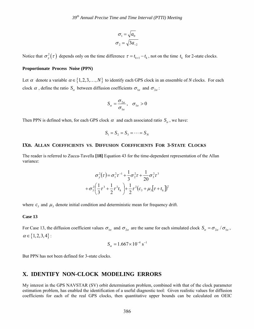
where and 3c 3μ denote initial condition and deterministic mean for frequency drift. Case 13 For Case 13, the diffusion coefficient values 1ασ and 2ασ are the same for each simulated clock 2 1/Sα α ασ σ= ,

{ }1, 2,3, 4α ∈ : 14 s 10667.1 −−×=αS

But PPN has not been defined for 3-state clocks. X. IDENTIFY NON-CLOCK MODELING ERRORS My interest in the GPS NAVSTAR (SV) orbit determination problem, combined with that of the clock parameter estimation problem, has enabled the identification of a useful diagnostic tool: Given realistic values for diffusion coefficients for each of the real GPS clocks, then quantitative upper bounds can be calculated on OEIC

386


magnitudes. These calculations require the use of a rigorous simulator. Existence of significant cross-correlations between GPS clock phase errors and other non-clock GPS estimation modeling errors enables significant aliasing into GPS clock phase estimates during operation of KF1 on real data. But given rigorous quantitative upper bounds on OEIC magnitudes, then significant violation of these bounds when processing real GPS pseudo-range and carrier-phase data identifies non-clock modeling errors related to the GPS estimation model. Modeling error candidates here include NAVSTAR orbit force modeling errors, ground antenna modeling errors (multipath), and tropospheric modeling errors. NAVSTAR orbit force modeling errors include those of solar photon pressure, albedo, thermal dump, and propellant outgassing. The accuracy of this diagnostic tool depends on the use of realistic clock diffusion coefficient values and a rigorous clock model simulation capability. XI. UNOBSERVABLE MEAN PHASE In an earlier version of my paper, I reported on KF1 validation results where clock S1 was specified as a TAI/UTC clock, external to the GPS clock ensemble consisting of S2, N1, and N2. This brought observability to S2, N1, and N2 clock states from GPS pseudo-range measurements, drove clocks S2, N1, and N2 immediately to the TAI/UTC timescale, and enabled a clean validation of my filter implementation. Also, it raised the question: Why not do the same thing for the real GPS clock ensemble? Discussions with Ed Powers (USNO) and Bill Feess (Aerospace Corporation) reveal that this approach was tried and discarded after the difficulty in recovery from an uplink hardware failure was blamed on the use of a single TAI/UTC Master Clock. This issue was resolved with Kenneth Brown’s introduction of the implicit ensemble mean. The mean phase (GPS Time) of the GPS clock ensemble will remain unobservable to GPS pseudo-range measurements in the USAF Kalman filter for the foreseeable future. NOTES

1. James R Wright is the architect of ODTK (Orbit Determination Tool Kit), a commercial software product offered by Analytical Graphics, Inc. (AGI).

2. Session IX, Paper 34. 3. According to Bill Feess, an improvement in control can be achieved by replacing the existing “bang-bang

controller” with a “proportional controller.” 4. See Zucca and Tavella [18] for concrete clock examples of 1,k kJ + and 1,k kQ + . 5. Observability is meaningful here only when processing simulated GPS pseudo-range data. 6. I apply sufficient process noise covariance for KF2 to mask the effects of double-precision computer

word truncation. Without this, KF2 does diverge. 7. Note that this is impossible using Kalman’s definition of observability. 8. Refer all times to a coordinate time, e.g., to GPS Time. Appropriate transformations between proper time

and coordinate time must be performed in the operational algorithms, but state estimate observability is independent of relativity, so observability can be defined and discussed independent of relativity.

9. This partition was introduced by Kenneth Brown [2]. REFERENCES

[1] T. W. Anderson, 1955, “The Integral of a Symmetric Unimodal Function over a Symmetric Convex Set and Some Probability Inequalities,” in Proceedings of the American Mathematical Society, Vol. 6, No. 2, pp. 170-176.

387


[2] K. R. Brown, 1991, “The Theory of the GPS Composite Clock,” in Proceedings of the Institute of Navigation – Global Positioning System, pp. 223-241.

[3] R. S. Bucy and P. D. Joseph, 1968, Filtering for Stochastic Processes with Applications to

Guidance (Interscience Publishers, New York). [4] William Feess, The Aerospace Corporation, private communications, 2006. [5] R. J. Gardner, 2002, “The Brunn-Minkowski Inequality,” Bulletin of the American Mathematical

Society, 30, No. 3, pp. 355-405. [6] Charles A. Greenhall, JPL/CIT, private communications, 2006-2007. [7] C. A. Greenhall, 2006, “A Kalman Filter Clock Ensemble Algorithm that Admits Measurement

Noise,” Metrologia, 43, S311-S321 [8] S. T. Hutsell, 1996, Relating the Hadamard Variance to MCS Kalman Filter Clock Estimation, in

Proceedings of the 27th Annual Precise Time and Time Interval (PTTI) Applications and Planning Meeting, 29 November-1 December 1995, San Diego, California, USA (NASA Conference Publication 3334), p. 293, Eqs. (8) and (9).

[9] R. E. Kalman, 1963, “New Methods in Wiener Filtering Theory,” in Proceedings of the First

Symposium on Engineering Applications of Random Function Theory and Probability, edited by J. L. Bogdanoff and F. Kozin (John Wiley & Sons, New York).

[10] J. S. Meditch, 1969, “Stochastic Optimal Linear Estimation and Control” (McGraw-Hill, New

York). [11] Edward Powers, private communications, 2006. [12] S. Sherman, 1955, “A Theorem on Convex Sets with Applications,” Annals of Mathematical

Statistics, 26, 763-767. [13] S. Sherman, 1958, “Non-Mean-Square Error Criteria,” IRE Transactions on Information Theory,

IT-4, 125-126. [14] E. M. Stein and R. Shakarchi, 2005, Real Analysis (Princeton University Press, Princeton). [15] J. R. Wright, 2005, “Sherman’s Theorem,” The Malcolm D. Shuster Astronautics Symposium, 13-15

June 2005, Grand Island, New York, AAS 05-451. [16] J. R. Wright, 2007, “GPS Composite Clock Analysis,” in Proceedings of TimeNav’07, the 21st

European Frequency and Time Forum (EFTF) Joint with 2007 IEEE International Frequency Control Symposium (IEEE-FCS), 29 May-1 June 2007, Geneva, Switzerland (IEEE Publication CH37839), pp. 523-528.

[17] J. R. Wright, 2008, “GPS Composite Clock Analysis,” to appear in the International Journal of

Navigation and Observation. [18] C. Zucca and P. Tavella, 2005, “The Clock Model and Its Relationship with the Allan and Related

Variances,” IEEE Transactions on Ultrasonics, Ferroelectrics, and Frequency Control, UFFC-

388


52, 289-296.

389


390

COMPOSITE CLOCKS WITH 3-STATE MODELS · 39th Annual Precise Time and Time Interval (PTTI) Meeting ....

Documents

Transcript of COMPOSITE CLOCKS WITH 3-STATE MODELS · 39th Annual Precise Time and Time Interval (PTTI) Meeting ....