COMPOSABLE MODELING AND DISTRIBUTED SIMULATION...
191
COMPOSABLE MODELING AND DISTRIBUTED SIMULATION FRAMEWORK FOR DISCRETE SUPPLY-CHAIN SYSTEMS WITH PREDICTIVE CONTROL by Dongping Huang A Dissertation Presented in Partial Fulfillment of the Requirements for the Degree Doctor of Philosophy ARIZONA STATE UNIVERSITY May 2008
Transcript of COMPOSABLE MODELING AND DISTRIBUTED SIMULATION...
COMPOSABLE MODELING AND DISTRIBUTED SIMULATION FRAMEWORK
FOR DISCRETE SUPPLY-CHAIN SYSTEMS WITH PREDICTIVE CONTROL
by
Dongping Huang
A Dissertation Presented in Partial Fulfillmentof the Requirements for the Degree
Doctor of Philosophy
ARIZONA STATE UNIVERSITY
May 2008
COMPOSABLE MODELING AND DISTRIBUTED SIMULATION FRAMEWORK
FOR DISCRETE SUPPLY-CHAIN SYSTEMS WITH PREDICTIVE CONTROL
by
Dongping Huang
has been approved
April 2008
Graduate Supervisory Committee:
Hessam S. Sarjoughian, ChairGerald C. GannodDaniel E. RiveraStephen S. Yau
ACCEPTED BY THE GRADUATE COLLEGE
ABSTRACT
Supply-chain networks such as semiconductor manufacturing systems exhibit a high de-
gree of structural and behavioral complexity. Simulation modeling concepts, approaches,
and tools are the primary means for analysis and design of intricate behavior and relation-
ships found in many of today’s supply-chain networks. A fundamental barrier in developing
rigorous simulation models of supply-chain systems is the necessity of using inherently dif-
ferent kinds of models and simulators. This is because no single modeling and simulation
framework has been shown to adequately represent, at a realistic level of detail, a supply-
chain system with tactical (short-term) control and strategic (long-term) planning policies.
Composition of disparate model types affords rigorous synthesis of complementary classes of
simulation, control, and optimization models. A novel framework using an approach called
Knowledge Interchange Broker (KIB) was developed for composing the distinct classes of
Discrete Event System Specification (DEVS), Model Predictive Control (MPC), and Linear
Optimization (LP) models. First, the KIB model composability approach was employed
to compose DEVS and MPC modeling formalisms. A KIBDEVS/MPC was developed and
used to create a hybrid DEVSJAVA/MATLAB prototype environment. The benefits of
simulating combined discrete-event and control-theoretic models was demonstrated against
a scaled prototypical semiconductor supply-chain system. Then, the KIBDEVS/LP/MPC was
developed to support composing models that can be described in DEVS, MPC, and LP
modeling formalism. This novel KIB provides a set of suitable message mappings and
transformations. A causal parallel execution protocol with logical time synchronization was
devised and used to develop a prototype distributed simulation framework for DEVSJAVA,
MATLAB, and OPLStudio, a linear optimization tool. The resulting simulation framework
iii

offers a basis for modeling complex discrete-part systems and, in particular, semiconductor
manufacturing supply-chain systems.
iv

To my parents
v

ACKNOWLEDGMENTS
First of all, I would like to give my sincerest gratitude to my dissertation advisors, Dr.
Hessam Sarjoughian, who introduced me to the fantastic world of modeling and simulation.
His professional guidance and encouragement on my research brought me so much insight
along the whole way to finish this dissertation.
I would like to thank all my committee members, Dr. Gerald Gannod, Dr. Daniel Rivera,
and Dr. Stephen Yau, for their invaluable advice on my research, the dissertation proposal,
and the oral defense. I would like to thank Dr. Dijiang Huang, for being the substitute in
my oral defense.
I would like to thank Dr. Karl Kempf at Intel Corporation, who guided me to understand
the practices of supply chain management in the semiconductor manufacturing industry.
I would like to thank Dr. Wenlin Wang, for his help and valuable discussion with me
regarding the advanced control theory.
I would like to thank Mr. Gary Godding and Mr. Gary Mayer, for their valuable
discussion with me on my research and for their advice. Their professional experiences were
helpful in my work.
I would like to thank all the members at ASU-ACIMS, for the useful discussion on my
research, for the support and the friendship.
I would like to express my wholehearted appreciation to my dearest parents and my
brother, for their endless love and encouragement. They shared the happiness of each of
my achievements and encouraged me when my spirits were down.
Finally, the financial support by National Science Foundation (Grant No: DMI-0432439)
and Intel Research Council is gratefully acknowledged.
vi
TABLE OF CONTENTS
Page
LIST OF TABLES . . . . . . . . . . . . . . . . . . . . . . . . . . . . . . . . . . . . . xi
LIST OF FIGURES . . . . . . . . . . . . . . . . . . . . . . . . . . . . . . . . . . . . xii
CHAPTER 1 INTRODUCTION . . . . . . . . . . . . . . . . . . . . . . . . . . . . 1
1.1. Problem Description . . . . . . . . . . . . . . . . . . . . . . . . . . . . . . . 1
1.2. Summary of Contributions . . . . . . . . . . . . . . . . . . . . . . . . . . . . 11
1.3. Dissertation Organization . . . . . . . . . . . . . . . . . . . . . . . . . . . . 11
CHAPTER 2 SEMICONDUCTOR MANUFACTURING SUPPLY-CHAIN SYS-
TEMS . . . . . . . . . . . . . . . . . . . . . . . . . . . . . . . . . . . . . . . . . . 14
2.1. Supply Chain Network . . . . . . . . . . . . . . . . . . . . . . . . . . . . . . 14
2.2. Semiconductor Manufacturing Supply Chain Network . . . . . . . . . . . . 16
2.3. Some Benchmark Problems in Semiconductor Manufacturing Supply Network 19
2.3.1. Bill of Material . . . . . . . . . . . . . . . . . . . . . . . . . . . . . . 20
2.3.2. Topology . . . . . . . . . . . . . . . . . . . . . . . . . . . . . . . . . 21
2.3.3. Domain View of a Semiconductor Manufacturing Supply-Chain System 22
2.4. Modeling and Simulation Technologies Used in Supply-Chain Systems . . . 25
CHAPTER 3 SEMICONDUCTOR SUPPLY-CHAIN MODELING AND SIMULA-
TION APPROACHES . . . . . . . . . . . . . . . . . . . . . . . . . . . . . . . . . 28
3.1. Process-Oriented Modeling and Simulation . . . . . . . . . . . . . . . . . . 28
3.1.1. System-Theoretic Discrete-Event Simulation . . . . . . . . . . . . . . 28
3.1.2. Agent-Based Modeling . . . . . . . . . . . . . . . . . . . . . . . . . . 33
3.2. Strategic Planning and Tactical Control . . . . . . . . . . . . . . . . . . . . 34
3.2.1. Operations Research Approach—Linear Programming for Optimization 34
vii
Page
3.2.2. Control Theoretic Approach—Model Predictive Control . . . . . . . 36
3.2.3. Other Approaches . . . . . . . . . . . . . . . . . . . . . . . . . . . . 38
3.3. Modeling and Simulation Environments . . . . . . . . . . . . . . . . . . . . 40
3.4. Summary . . . . . . . . . . . . . . . . . . . . . . . . . . . . . . . . . . . . . 41
CHAPTER 4 MULTIFACETED MODEL COMPOSITION AND DISTRIBUTED
SIMULATION . . . . . . . . . . . . . . . . . . . . . . . . . . . . . . . . . . . . . 42
4.1. Modeling Formalism Composition Concepts and Approaches . . . . . . . . . 42
4.1.1. Mono- and Super-Formalism Modeling . . . . . . . . . . . . . . . . . 43
4.1.2. Meta-Formalism Modeling . . . . . . . . . . . . . . . . . . . . . . . . 45
4.1.3. Multi-Formalism Modeling . . . . . . . . . . . . . . . . . . . . . . . 46
4.2. Software Component Specification and Interaction . . . . . . . . . . . . . . 46
4.3. Service-Oriented Interoperation . . . . . . . . . . . . . . . . . . . . . . . . . 48
4.3.1. High-Level Architecture . . . . . . . . . . . . . . . . . . . . . . . . . 49
4.3.2. Web Services . . . . . . . . . . . . . . . . . . . . . . . . . . . . . . . 50
4.3.3. Grid Services . . . . . . . . . . . . . . . . . . . . . . . . . . . . . . . 51
4.3.4. Other Approaches . . . . . . . . . . . . . . . . . . . . . . . . . . . . 53
4.4. Parallel and Distributed Simulation . . . . . . . . . . . . . . . . . . . . . . . 53
4.5. Summary . . . . . . . . . . . . . . . . . . . . . . . . . . . . . . . . . . . . . 54
CHAPTER 5 KNOWLEDGE INTERCHANGE BROKER FOR MODELING COM-
POSITION . . . . . . . . . . . . . . . . . . . . . . . . . . . . . . . . . . . . . . . 56
5.1. Broker System Architecture Pattern . . . . . . . . . . . . . . . . . . . . . . 56
5.2. Related work . . . . . . . . . . . . . . . . . . . . . . . . . . . . . . . . . . . 58
5.2.1. KIB in DEVS/RAP . . . . . . . . . . . . . . . . . . . . . . . . . . . 58
viii
Page
5.2.2. KIB in DEVS/LP . . . . . . . . . . . . . . . . . . . . . . . . . . . . 62
5.3. Conceptual Specification of KIB . . . . . . . . . . . . . . . . . . . . . . . . 66
5.3.1. Structural Composition Specification . . . . . . . . . . . . . . . . . . 67
5.3.2. Behavioral Composition Specification—Time Synchronization . . . . 72
5.3.3. Control Scheme for Composite Model Execution . . . . . . . . . . . 75
5.3.4. Software Design Perspective . . . . . . . . . . . . . . . . . . . . . . . 80
5.4. Summary . . . . . . . . . . . . . . . . . . . . . . . . . . . . . . . . . . . . . 81
CHAPTER 6 BI-FORMALISM COMPOSITION OF DISCRETE-EVENT SIMULA-
TION AND MODEL PREDICTIVE CONTROL . . . . . . . . . . . . . . . . . . 82
6.1. DEVS Modeling for Semiconductor Manufacturing Physical Process . . . . 82
6.1.1. Semiconductor Supply-Chain Model Specification . . . . . . . . . . . 87
6.2. Predictive Optimization-Based Tactical Control . . . . . . . . . . . . . . . . 97
6.3. Hybrid DEVS/MPC using KIB . . . . . . . . . . . . . . . . . . . . . . . . . 101
6.3.1. Structural Composition . . . . . . . . . . . . . . . . . . . . . . . . . 102
6.3.2. Behaviorial Composition . . . . . . . . . . . . . . . . . . . . . . . . . 106
6.4. Prototype DEVS/MPC KIB with Sequential Control Scheme . . . . . . . . 111
6.5. Experimental Results and Analysis . . . . . . . . . . . . . . . . . . . . . . . 114
6.5.1. Simulation Testbed . . . . . . . . . . . . . . . . . . . . . . . . . . . . 115
6.5.2. Manufacturing Process Simulation Validation . . . . . . . . . . . . . 116
6.5.3. Hybrid DEVS/MPC Simulation Validation . . . . . . . . . . . . . . 118
6.5.4. Execution Time vs. Accuracy Analysis . . . . . . . . . . . . . . . . . 125
6.6. Summary . . . . . . . . . . . . . . . . . . . . . . . . . . . . . . . . . . . . . 126
ix
Page
CHAPTER 7 A DISTRIBUTED FRAMEWORK FOR HYBRID DISCRETE-
EVENT PROCESS SIMULATION WITH MIXED OPTIMIZATION AND MODEL
PREDICTIVE CONTROL . . . . . . . . . . . . . . . . . . . . . . . . . . . . . . 128
7.1. KIB Structural Composition Specification . . . . . . . . . . . . . . . . . . . 130
7.1.1. DEVS Model Interface Specification . . . . . . . . . . . . . . . . . . 131
7.1.2. Decision Model Interface Specification . . . . . . . . . . . . . . . . . 133
7.1.3. Complex Data Type Definition . . . . . . . . . . . . . . . . . . . . . 135
7.1.4. Message Transformation Specification . . . . . . . . . . . . . . . . . 136
7.2. KIB Behavioral Composition Specification . . . . . . . . . . . . . . . . . . . 140
7.2.1. DecisionProxy Interface . . . . . . . . . . . . . . . . . . . . . . . . . 143
7.2.2. DEVSProxy Interface . . . . . . . . . . . . . . . . . . . . . . . . . . 144
7.3. Parallel Execution Control . . . . . . . . . . . . . . . . . . . . . . . . . . . . 149
7.4. Software Design of Hybrid DEVS/LP/MPC Distributed Simulation Framework158
7.4.1. KIB Interface Compoments . . . . . . . . . . . . . . . . . . . . . . . 159
7.4.2. KIB Core Components . . . . . . . . . . . . . . . . . . . . . . . . . . 162
7.5. Summary . . . . . . . . . . . . . . . . . . . . . . . . . . . . . . . . . . . . . 163
CHAPTER 8 CONCLUSION AND FUTURE WORK . . . . . . . . . . . . . . . . 165
8.1. Conclusions . . . . . . . . . . . . . . . . . . . . . . . . . . . . . . . . . . . . 165
8.2. Future Work . . . . . . . . . . . . . . . . . . . . . . . . . . . . . . . . . . . 168
REFERENCES . . . . . . . . . . . . . . . . . . . . . . . . . . . . . . . . . . . . . . . 170
x
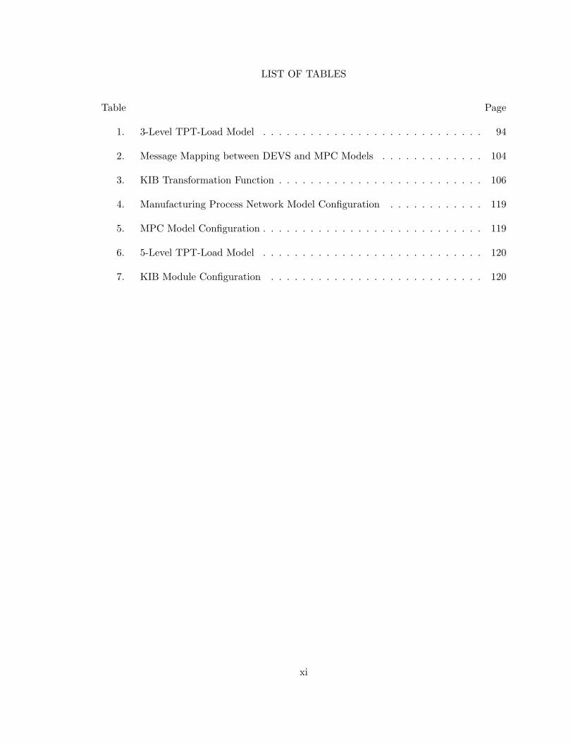
LIST OF TABLES
Table Page
1. 3-Level TPT-Load Model . . . . . . . . . . . . . . . . . . . . . . . . . . . . 94
2. Message Mapping between DEVS and MPC Models . . . . . . . . . . . . . 104
3. KIB Transformation Function . . . . . . . . . . . . . . . . . . . . . . . . . . 106
4. Manufacturing Process Network Model Configuration . . . . . . . . . . . . 119
5. MPC Model Configuration . . . . . . . . . . . . . . . . . . . . . . . . . . . . 119
6. 5-Level TPT-Load Model . . . . . . . . . . . . . . . . . . . . . . . . . . . . 120
7. KIB Module Configuration . . . . . . . . . . . . . . . . . . . . . . . . . . . 120
xi
LIST OF FIGURES
Figure Page
1. Simplified Semiconductor Manufacturing Flows . . . . . . . . . . . . . . . . 17
2. A Sample of Semiconductor Supply-Chain BOM Mapping . . . . . . . . . . 20
3. A Sample of Semiconductor Supply-Chain Topology . . . . . . . . . . . . . 22
4. Sub-Systems of a Semiconductor Manufacturing Supply-Chain System . . . 23
5. DEVS Simulation Engine Structure . . . . . . . . . . . . . . . . . . . . . . . 31
6. MPC Structure . . . . . . . . . . . . . . . . . . . . . . . . . . . . . . . . . . 38
7. DEVS/RAP KIB Design . . . . . . . . . . . . . . . . . . . . . . . . . . . . . 61
8. Multi-Formalism Modeling Composability Framework Using KIB Concept . 66
9. Hierarchy of Message Transformation . . . . . . . . . . . . . . . . . . . . . . 69
10. Sequential Execution Scheme . . . . . . . . . . . . . . . . . . . . . . . . . . 77
11. Parallel Execution Scheme . . . . . . . . . . . . . . . . . . . . . . . . . . . . 79
12. Prototypical Semiconductor Manufacturing Process Network . . . . . . . . 83
13. Local Control Policy for Inventory . . . . . . . . . . . . . . . . . . . . . . . 86
14. Simplified State Diagram of Supply-Chain Node DEVS Model . . . . . . . . 88
15. Processing Procedure in Factory Model . . . . . . . . . . . . . . . . . . . . 88
16. Inventory-Factory Coupled Model . . . . . . . . . . . . . . . . . . . . . . . . 94
17. Data/Control Interaction in DEVS and MPC Models . . . . . . . . . . . . . 97
18. Composing Discrete-Event System Specification and Model Predictive Con-
trol Models with Knowledge Interchange Broker . . . . . . . . . . . . . . . . 102
19. Event Scheduling for a Coupled Inventory/Factory Model and KIBDEVS/MPC 110
20. DEVS/MPC Conceptual Software Architecture . . . . . . . . . . . . . . . . 111
21. KIB Composition Specification . . . . . . . . . . . . . . . . . . . . . . . . . 113
xii
Figure Page
22. Sequence Diagram of the Interaction between DEVS and MPC Models via
the KIB . . . . . . . . . . . . . . . . . . . . . . . . . . . . . . . . . . . . . . 114
23. Combined DEVS/MPC Simulation Testbed . . . . . . . . . . . . . . . . . . 115
24. Fab/Test1 Starts and Actual Outs with Different Lot Sizes . . . . . . . . . . 117
25. Simulation Plots of Inventory Levels and Factory Starts with Customer Pro-
file A . . . . . . . . . . . . . . . . . . . . . . . . . . . . . . . . . . . . . . . . 121
26. Effect of Varying fa on Inventory and Factory Starts with 5 TPT-Load Level 124
27. Effect of Varying TPT-load on Inventory and Factory Starts with fa = 0.01 124
28. Effect of Varying TPT-load on Inventory and Factory Starts with fa = 0.05 125
29. Average DEVS and DEVS/MPC Execution Times . . . . . . . . . . . . . . 126
30. Combined Supply Chain Manufacturing System with Tactical Controller and
Strategic Planner . . . . . . . . . . . . . . . . . . . . . . . . . . . . . . . . . 129
31. KIB Message Transformation . . . . . . . . . . . . . . . . . . . . . . . . . . 141
32. KIB Model and Execution . . . . . . . . . . . . . . . . . . . . . . . . . . . . 143
33. Structure of the DEVProxy DEVS Model . . . . . . . . . . . . . . . . . . . 145
34. Simplified State Diagram of DEV SProxy DEVS Model . . . . . . . . . . . 146
35. KIB Executor— Parallel Execution Control . . . . . . . . . . . . . . . . . . 156
36. KIBDEV S/LP/MPC Interface Design . . . . . . . . . . . . . . . . . . . . . . . 159
37. Sequence Diagram for the Interaction of the KIB and Decision Interface . . 161
38. KIB Components Design . . . . . . . . . . . . . . . . . . . . . . . . . . . . . 162
39. Distributed DEVS/LP/MPC Simulation Deployment . . . . . . . . . . . . . 164
xiii
CHAPTER 1
INTRODUCTION
For large-scale manufacturing supply-chain systems such as semiconductor manufacturing
systems, some of the main goals of the management are to achieve effective and efficient
manufacturing operations over relatively long periods of time, satisfy the growing desire
for product customization, adjust fast on-demand change for just-in-time delivery, and
maximize profits. Management of such complex network systems demonstrates the potential
of coordinating organizational units and integrating diverse flows such as those of materials,
information and finance with different levels of planning and controlling along the supply
chain. Simulation technology has been widely used to analyze supply chain activities and
evaluate supply chain management.
1.1 Problem Description
There exist a variety of activities along the supply-chain network systems. The activities
exhibit distinct features. It is desired to develop a simulation modeling composability
framework for synthesizing disparate kinds of modeling formalisms (e.g., process dynamics
and decision policies for supply-chain systems) to achieve simulation-based analysis and
design. In the research of modeling composability and simulation interoperability, a number
of key barriers have been identified [62]: to improve system integration capability, to improve
model reliability and robustness, and improve model reusability.
More specifically, the barriers addressed above result in a number of challenges to be
tackled in the context of decision making for efficient operations of semiconductor man-
ufacturing supply-chain systems: (i) combinational complexity of the problems—multiple
end or intermediate products, multiple echelons, and multiple sites, (ii) stochastic manufac-
turing processes—variable throughput time, stochastic yield, and uncertain outputs from
a factory, (iii) stochastic demand—hard to forecast, (iv) complex mapping of the fan-out
2
and fan-in products, (v) non-linearity of many of the key cause-effect relationships, and (vi)
sophisticated dealing with financial aspects of the problem—trade-off of minimizing costs
vs. maximizing revenues and balance on maximizing short-term profits vs. maximizing
long-term profits.
Given the challenges and broad spectrum of holistic semiconductor manufacturing supply-
chain systems, many well established and contemporary research fields have been attracted
to seek for approaches and techniques to help with problem analysis and system design
development. The research on modeling manufacturing supply-chain system can be in-
formally categorized from two perspectives: physical manufacturing process modeling and
strategic/tactical/operational decision making. The physical manufacturing process mod-
eling is focused on developing models to capture supply-chain manufacturing dynamics,
whereas the decision making concentrates on improving the operations of a manufacturing
supply-chain system which accounts for achieving efficiency, delivering the right products
at the right time while satisfying the financial goals. Apparently the two perspectives are
closely associated with each other—manufacturing process modeling feeds the decision mak-
ing with the process dynamic information and the decision making modeling provides the
process models with operation commands.
Two modeling paradigms—analytical and simulation-based—are widely used for speci-
fying a supply-chain system’s physical dynamics and decision making. In the analytical
methods, the dynamics of the supply-chain system models are derived using mathematical
theories including well-known queueing and probabilistic methods. Mathematical program-
ming such as Linear Programming and Mixed Integer Programming are popular optimiza-
tion techniques in the operations research community to formulate tactical and strategic
decision models. In comparison with the analytical methods, simulation-based approaches
3
are based on the concepts and theories that are closely related to system and computing
theories. The main objectives of simulation include analyzing detailed system dynamics,
evaluating decision policies, and facilitating system validation and verification that closely
reflects real-world systems.
The physical manufacturing processes and the decision making must complement each
other to help formulate the problems and solutions of the intertwined operations and man-
agement of real-world semiconductor manufacturing supply-chain systems. The process
simulation models can represent realistic manufacturing dynamics but by itself are not suit-
able for supply-chain management. Simulation models need to be provided with controls
by the decision models. In contrast, the decision models must have accurate dynamic data
that is grounded in the manufacturing simulation in order to produce appropriate controls
and decision policies. This is necessary for realistic manufacturing process dynamics which
cannot be appropriately modeled inside the decision models. It needs to be aware that the
process simulation models generally represent short-term (hourly or daily) manufacturing
processes, whereas the decision models formulate long-term (weekly or monthly) decision
polices.
A variety of modeling approaches have been applied in simulating physical manufactur-
ing processes. Simulation-based modeling approaches provide a practical basis for studying
supply-chain problems. Details of supply-chain simulation models directly affect their anal-
ysis [14, 91, 107, 19]. Furthermore, realistic (intricate) simulation models of discrete sys-
tems, especially specifying interaction with other types of models are essential in designing
high-level robust control scheme [33].
The formulation of modeling approaches are rooted in abstracting manufacturing pro-
cesses in terms of specification of time as discrete-event, discrete-time, continuous, or some
4
combination thereof. Among these, the discrete-event modeling paradigm has been com-
monly used to describe the discrete processes at different levels of abstractions—i.e., shop-
floor operations within a manufactory, enterprise-level processing along the entire supply-
chain, or across enterprises([26, 37, 58]). More recently, distributed discrete-event simulation
frameworks have been proposed for large-scale, interoperable simulations [43]. Discrete-
Event Simulation (DES) has been generally considered suitable for modeling and simulat-
ing physical manufacturing behaviors in semiconductor supply-chain systems. In addition,
some discrete-event simulation models are as well used for controlling the real-time physical
processes in stead of for system analysis and evaluation [69]. Among the DES approaches,
Discrete EVent System Specification (DEVS) is a modeling formalism for describing (dis-
crete and continuous) dynamical systems as discrete-event models [104]. Developed based
on system theoretic concepts, DEVS formalism uses mathematical set theory and provides
a framework to support model development with well-defined structural and behavioral
specifications and a sound simulation algorithm. This framework is extended with object-
oriented abstraction, encapsulation, modularity and hierarchy concepts and constructs [106].
The simulation protocol enforces causality, concurrency, and timing among DEVS models
so as to ensure that the dynamic behaviors of the models are executed properly. It has been
demonstrated that DEVS can formulate complex physical processing dynamic behaviors for
the semiconductor supply-chain systems [84].
Some researchers have been using the agent-based modeling approach to adapt loosely
coupled component-based concepts for describing and simulating supply-chain dynam-
ics [23]. In this approach, the supply chain entities—e.g., manufacturers, warehouses,
distributors, customers, and even the decision makers—are viewed as constituent agents
each of which is defined to have its own responsibilities and as well have loosely coupled re-
5
lationship with other agents to specify complex interacting dynamics along the supply-chain
systems. The agents are then mapped into software components which can be executed and
thus allow for analysis of individual and collective dynamic behaviors of manufacturing
processes. The agent-based modeling approach and its realization, however, doesn’t have
a universally accepted theory. For instance, it doesn’t have well-defined timing concept
which is a key factor in the modeling and simulation community. It can not only weaken its
capabilities of specifying varying levels of complexity of the process dynamics, but also limit
its interactions with other types of models (e.g., model-based controller or optimization)
where time-based synchronization is crucial.
The formulation of decision policies is an active research area for managing supply-chain
systems. Generally there are three hierarchical levels of decisions or controls—strategic,
tactical, and operational, given different decision time horizons. At the strategic level, the
decisions are generally for manufacturing network structure, facility location, and outsourc-
ing scheme. Production and distribution planning and safety stock are managed via the
tactical control. Order replenishment, transportation planning, lot-sizing, and machine-
scheduling are considered as operational controls.
Different types of information flows (e.g., production information, and financial informa-
tion) are involved between the manufacturing facilities and decision policies. Therefore,
the decision models need to primarily depend on quantitative methods. In the operations
research community, mathematical programming has been widely applied to coordinate the
flows among the supply-chain entities for model developing and problem solving. Typical
optimization techniques include Linear and Mixed Integer Programming, Constraint Pro-
gramming, and Genetic Algorithm. In the research field for semiconductor manufacturing
supply-chain system management, Linear Programming optimization has been used to for-
6
mulate strategic planning problems for allocating capacity to satisfy customer demands
while minimizing costs and maximizing profits. For example, in [38] the core formula-
tion of LP is based on mass balance and capacity constraints and an objective function
that includes minimizing costs and maximizing revenues. The strategic planning in the
LP formulism are assumed to be deterministic. Due to the unavoidable stochasticity of
supply and demand, stochastic programming techniques have been used to account for un-
certainty. For instance, Multistage Stochastic Linear Programming (MSLP) with scenario
analysis was proposed for strategic semiconductor capacity planning [8]. However, it is
generally costly by using stochastic programming to obtain optimal solutions, since many
”what-if” scenarios have to be simulated and analyzed by highly skilled professionals [38].
Recently, some researchers have been using control-theoretic concepts to model decision
policies and then apply it to the supply-chain system. Model Predictive Control (MPC)
has been considered to be an effective method to handle time-varying stochasticity inherent
in controlling and managing supply-chain systems [5, 95, 94]. It has been shown that
MPC can be used successfully in tactical control to track inventory targets while satisfying
customer demands for products’ life-cycles starting from processing raw materials to delivery
to the customers. For example, manufacturing starts and inventory levels are controlled
over several months—e.g. spanning several times of the products’ producing cycles. The
advantages of using MPC for supply chain management lies in its optimization capacity and
control capacity [94]: as an optimizer, it can maximize or minimize an objective function
which can represent a suitable measure for manufacturing supply-chain performance; as a
controller, it can be tuned to achieve stability, robustness, and efficiency in the presence of
plant/model mismatch, disturbance and uncertainty.
7
Solving both the mathematical programming models and control-theoretic models re-
quires great computation capability and may be time-consuming.
Manufacturing operations account for a series of processes with feed-forward and feed-
back interactions among the supply-chain entities to generate products from raw materials.
Individual and collective processes are in part controlled by local controls that are directly
tied to the manufacturer’s internal, short-term constraints such as meeting weekly demands
given resource availability, production capacity, and schedule constraints. Strategic and
tactical supply-chain management focuses on delivery of products to the customer given
constraints external to the manufacturing. The manufacturing processes, in addition to the
local controls, are subject to the external influences which may impose long-term constraints
such as an unexpected increase or decline in market demands.
Combined process simulation and decision control can be modeled in a homogeneous
or heterogeneous environment. In particular, given the variety of decision tasks in the
supply-chain management, no single modeling formalism can appropriately specify the key
aspects of discrete processes, control scheme, and their interactions. In the semiconduc-
tor supply-chain systems, modeling and simulation of the physical processes dynamics are
fundamentally different from modeling and solving logical decision controls. More recently,
synthesis of these complementary modeling approaches has been attracting researchers and
practitioners (e.g., [91, 101, 23]).
It is common to have different modeling techniques used for tackling specific discrete pro-
cessing or decision making for supply-chain systems. For instance, discrete-event simulation
and linear programming models are combined in such a way that the state of the process
model dynamics is consumed iteratively by a decision controller which in turn provides a
plan to the process models [34]. Another approach uses MPC models and discrete-time
8
simulation models mainly to propose a flexible formulation of MPC modeling for daily tac-
tical control in supply-chain management in semiconductor manufacturing [95]. The goal
of this research has been to develop concepts and devise MPC models for discrete-part
semiconductor manufacturing supply-chain systems. The MPC formulation and the man-
ufacturing process simulation models were modeled in term of user-defined block models
in the SIMULINK/MATLAB [48] to tackle a set of representative and challenging prob-
lems occurring in the semiconductor manufacturing. Both the MPC and process simulation
models are described as discrete-time models. How time should be advanced needs to be
specified in the models. In this work, no explicit interactions are defined between the MPC
and the process simulation models. The integration of the models and their execution is
achieved via MATLAB block models.
The synthesis of disparate modeling techniques can be achieved at the different levels of
abstraction—software programming, interoperability techniques, and multi-model compos-
ability approach. For example, there have been some researches (e.g., [101, 88])in which
software-centric middleware technology or ad-hoc software engineering concepts and pro-
gramming techniques including XML models are utilized to achieve model interactions. High
Level Architecture (HLA) [29], on the other hand, relies on interoperability concepts and
techniques. HLA supports creating federations of disparate simulations using a combination
of distributed simulation protocols and object-oriented modeling concepts and techniques
[80]. Each of these approaches has its own advantages and disadvantages. For instance,
when models to be composed belong to the discrete-event, discrete-time, and continuous
formalisms, it is beneficial to use the simplicity and rigor afforded by the DEVS framework
to develop hybrid continuous/discrete simulation models [41] or to use middleware technolo-
gies to interact modern and legacy simulation models and execute them in the distributed
9
settings [7, 103]. All these approaches offer some advantages, but none handles modeling
the so-called meta-formalism [60] and poly-formalism composability [81].
To formalize complementary and unique aspects of complex interacting systems, a gen-
eral modeling composition framework referred to as Knowledge Interchange Broker (KIB)
was proposed to achieve model composability via formalizing the composition of disparate
models [79]. The conceptual basis of this approach is that the data and control specified in
the distinct formalisms offers specific syntax and semantic contexts which are ideally com-
posed independent of software design and programming language choices. In particular,
the interactions among disparate models are specified as a pair: (i) model composability at
the level of modeling formalisms and (ii) simulation interoperability at the level of abstract
simulation protocols [80].
The first realization of the KIB framework focused on synthesizing models described in the
DEVS and the Reactive Action Planning (RAP) formalism [79]. The RAP is an agent-based
modeling approach where logic-based reasoning is deemed important [15]. The resulting
KIBDEVS/RAP demonstrated how input and output message transformations and execution
control can be explicitly specified [77]. The system was designed and implemented using
object-oriented technologies without relying on the limitations posed by the (low-level and
high-level) interoperability concept and supported with distributed simulation/middleware
technologies or socket communication constructs [30].
Following research has been focused on the semiconductor domain with the emphasis
on complex transformations. The KIBDEVS/LP has been introduced to compose the class
of DES and Linear Programming models [27, 25]. This work provides a suite of domain
-specific configurable data transformations that conform to the operations of prototypical
semiconductor manufacturing supply-chain systems. A key aspect of this work is realistic
10
modeling of semiconductor supply-chain manufacturing processes and decision policies in
terms of detailed discrete-event simulation models and large-scale linear optimization models
respectively. The KIBDEVS/LP specified the interaction between discrete processes and
decision policies for the class of manufacturing supply-chain systems. DEVSJAVA and
OPLStudio are used to build a hybrid DEVS simulation and LP optimization testbed for
analyzing and operating realistic semiconductor supply chain systems [28, 25].
The KIB multi-formalism model composability framework introduces a novel modeling
capability beyond what can be achieved using software-centric concepts or interoperability
techniques. By considering the realistic intricateness in the semiconductor manufactur-
ing supply-chain system management, there are three main challenges in the existing KIB
modeling composability framework.
� How to use the KIB approach to compose discrete-event manufacturing processes and
predictive control models that includes not only optimization models but predictive
models as well.
� How to define the KIB specification to support specification of the interactions among
discrete-event processes, MPC as tactical control policies, and LP as strategic decision
planning, the three distinct modeling approaches. Furthermore, the analysis of the
complexity on the KIB specification given the increasing number of participating
disparate modeling formalisms is desired to be studied.
� How to specify the KIB execution protocol to ensure the interactions among the dis-
parate models and consequently the holistic composite model are correctly executed,
particularly in term of concurrency, causality, and timing.
11
1.2 Summary of Contributions
The main contributions of the dissertation are as follows:
� Designed a new Knowledge Interchange Broker (KIB)—KIBDEVS/MPC to support
composing the Discrete EVent Simulation(DEVS) and Model Predictive Control
(MPC) models.
– Developed a hybrid DEVS/MPC simulation testbed using DEVSJAVA discrete-
event simulator and MATLAB/SIMULINK tool to support experimentations of
DEVS and MPC models via KIBDEVS/MPC.
– Demonstrated the capabilities of the model composition approach through simu-
lations of a prototypical semiconductor manufacturing supply-chain system. The
experimental testbed provides the capabilities for observing and analyzing how
discrete-event processes and control policies affect each other.
� Extended the KIBDEVS/MPC to create a new KIBDEVS/LP/MPC for composing models
that are described in DEVS, MPC, and Linear Programming (LP) modeling for-
malisms.
– Devised a protocol for executing multiple disparate models in parallel with logical
time synchronization.
– Developed a prototype distributed simulation framework using DEVSJAVA,
MATLAB/SIMULINK, and OPL Studio environments in which the disparate
models as well as the KIB can be executed concurrently.
1.3 Dissertation Organization
In the following, a brief overview of each chapter in the dissertation is given.
12
In Chapter 1, the problems and challenges in the modeling and simulation of the holistic
semiconductor manufacturing supply-chain systems were addressed. We reviewed some rel-
evant and important aspects of describing manufacturing supply-chain systems, presented a
brief discussion on the background, reviewed the related work, and outlined the organization
of the dissertation.
In Chapter 2, we will begin with the background of supply-chain systems and particularly
the semiconductor manufacturing supply-chain systems. Then we will focus on a set of
benchmark problems existing in the domain of semiconductor manufacturing supply-chain
network. It will be followed by a brief discussion of the related modeling and simulation
technologies in the supply-chain systems.
In Chapter 3, we will introduce a set of existing modeling and simulation approaches used
for semiconductor manufacturing supply-chain systems. These modeling and simulation
approaches are discussed from both the process-oriented and decision-oriented perspectives,
which provide necessary links for the later chapters. Specifically, the specification of DEVS,
LP, and MPC will be discussed in detail.
In Chapter 4, the concepts and principles of the existing multifaceted model composition
and distributed simulation will be particularly introduced and reviewed. A brief discussion
of the software engineering techniques with regard to the software interoperation will be
given thereafter.
In Chapter 5, a detailed discussion on the Knowledge Interchange Broker specification
will be given. The concept and principle of the KIB will be introduced and compared with
the existing Broker software design pattern. Then the KIBDEVS/RAP and KIBDEVS/LP, as
related work, will be reviewed from both the specification and software design viewpoints.
After the related work, the conceptual specification—structural specification and behavioral
13
specification—of KIB will be addressed in detail. The following will be a discussion of the
control scheme on the composite model execution.
In Chapter 6, we will give a detailed specification of KIBDEVS/MPC for bi-formalism com-
position and demonstrate the correctness of the KIBDEVS/MPC. First, a set of representative
DEVS models will be specified to model the semiconductor manufacturing processes. Sec-
ond, a detailed description of MPC model for tactical control will be given. Third, the
specification of KIBDEVS/MPC will be provided. These specifications will be followed by the
software design of the prototypical simulation testbed which is built by using DEVSJAVA
as discrete-event simulator and MATLAB/SIMULINK tool as MPC solver. At last, a set
of experimental scenarios with the result analysis will be discussed aiming at validating
the process simulation models and verifying the correctness of the composite model and its
execution.
In Chapter 7, the extended KIB specification for composite DEVS, MPC, and LP model
will be provided. This specification will account for flexible message mapping and trans-
formation, timing specification, and causal parallel execution control. Then the software
design of the prototype environment will be discussed.
In Chapter 8, the summary of contributions, conclusions and future work will be pre-
sented.
CHAPTER 2
SEMICONDUCTOR MANUFACTURING SUPPLY-CHAIN SYSTEMS
Impressive achievements from the adoption of advanced supply chain management tech-
niques have been shown in many cases. These achievements demonstrate the potential of
coordinating organizational units and integrating diverse flows such as those of materials,
information and finance with different levels of planning and controlling along the supply
chain. The characteristics of such complex networks also bring up questions regarding sup-
ply chain management. What approach is the most appropriate to managing the complex
network? How can we ensure a specific plan or decision will work well enough before it is
actually applied to the real system? Supply chain management has attracted different fields
of researchers and engineers.
2.1 Supply Chain Network
There have been various definitions of a supply chain as well as supply chain management
in the past several years. A supply chain can be defined as “all the activities involved in
delivering a product from raw materials through to the customer, including sourcing raw
material and parts, manufacturing and assembly, warehousing and inventory tracking, order
entry and order management, distribution across all channels, delivery to the customers,
and the information systems necessary to monitor all of these activities”, while the goal
of supply chain management “is to coordinate and integrate all of these activities into a
seamless process” [46].
A typical supply chain is comprised of two main business processes: material management
(inbound logistics) and physical distribution (outbound logistics) [57]. The former supports
a complete cycle of material flow from the purchase and internal control of production
material, to the planning and control of works-in-progress, to the warehousing, and to
shipping and distributing of final products, while the latter encompasses all the outbound
15
logistic activities related to providing customer services. A supply chain is not merely a
linear chain, but a web of multiple business networks and relationships. There may be
multiple stakeholders consisting of various suppliers, manufacturers, distributors, third-
party logistics providers, retailers, and customers in the supply chain network.
A supply chain network can be characterized as a number of quite different but interre-
lated “flows” including physical, financial, decision, and information data flows [72]. The
physical flow represents the physical goods being produced, stored, and shipped. The fi-
nancial flow concerns the payment for the materials and services required and products
supplied. The decision flow provides directions to the physical system based on the data
available on the physical flow, the advice from the financial flow, and the decision policies.
The information flow holds the past, present and forecasted future states of the physical
and financial flows.
In general, supply chain management involves hierarchical levels of managements such as
strategic advanced planning and tactical operational control. To coordinate and integrate all
the activities, supply chain management heavily depends on accurate and timely information
that can be shared among the supply chain members. Supply chain models can provide
users access to this information. Because of the broad spectrum of a supply chain, no
homogeneous modeling approach can capture all the aspects of supply chain processes and
management. Therefore, an appropriate modeling approach must be chosen to specify
particular behaviors of the supply chain.
In addition, simulation technology has been widely used to analyze supply chain activ-
ities and evaluate supply chain management. In today’s fast changing market, simulation
technology must have high fidelity, flexibility, and scalability. It should be able to address
the entire cycle, beginning with simulation modeling, and it should also support model val-
16
idation, simulation deployment, data input, simulation execution, planning and scheduling
control and optimization, control implementation and execution, output data collection and
analysis, and finally, model maintenance.
2.2 Semiconductor Manufacturing Supply Chain Network
In a broad sense a supply chain is inter-organizational, whereas in a narrow sense a supply
chain is intra-organizational. For a manufacturing company, intra-organizational supply
chain management plays a critical role in the enterprise’s activities. The semiconductor
industry is one typical example of manufacturing enterprises with its own specialties: it has
manufacturing processes with much uncertainty; it covers a complete supply chain includ-
ing suppliers, manufacturers, inventories, shipping, a wide variety of products, and large
demand variability with a corresponding uncertainty of demand forecasts. For example, In-
tel Corporation, an international high-volume manufacturer of semiconductors, maintains
a core manufacturing supply chain network of logic, memory, and communication prod-
ucts (among others). Although greatly simplified for the purpose of our research, several
benchmark semiconductor problems presented represent tens of billions of dollars in annual
sales to hundreds of millions of end customers for tens of thousands of diverse products.
The most sophisticated current logic products integrate roughly 250 million transistors on
a silicon die whose size is only about that of the average human thumbprint, and have
continuously increased in complexity in accordance with Moores law for over 30 years. The
factories required to manufacture products of such sophistication currently cost roughly 3
billion dollars to construct and outfit, and they have continued to become more expensive
with every generation of decreasing transistor size [38].
17
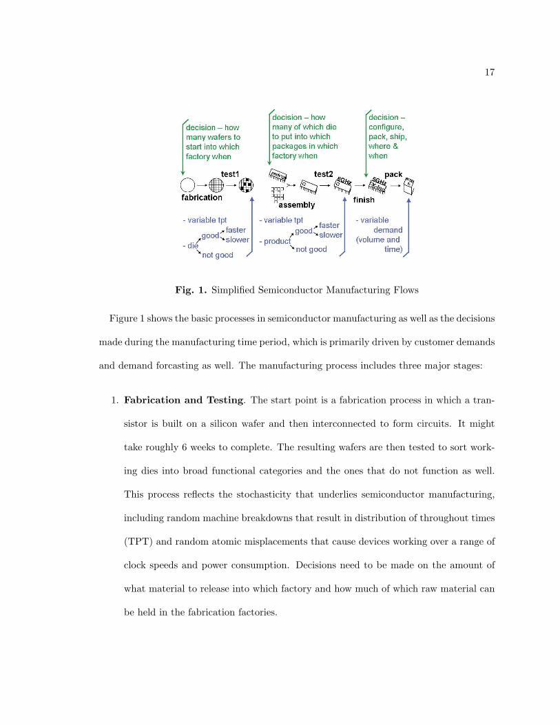
Fig. 1. Simplified Semiconductor Manufacturing Flows
Figure 1 shows the basic processes in semiconductor manufacturing as well as the decisions
made during the manufacturing time period, which is primarily driven by customer demands
and demand forcasting as well. The manufacturing process includes three major stages:
1. Fabrication and Testing. The start point is a fabrication process in which a tran-
sistor is built on a silicon wafer and then interconnected to form circuits. It might
take roughly 6 weeks to complete. The resulting wafers are then tested to sort work-
ing dies into broad functional categories and the ones that do not function as well.
This process reflects the stochasticity that underlies semiconductor manufacturing,
including random machine breakdowns that result in distribution of throughout times
(TPT) and random atomic misplacements that cause devices working over a range of
clock speeds and power consumption. Decisions need to be made on the amount of
what material to release into which factory and how much of which raw material can
be held in the fabrication factories.
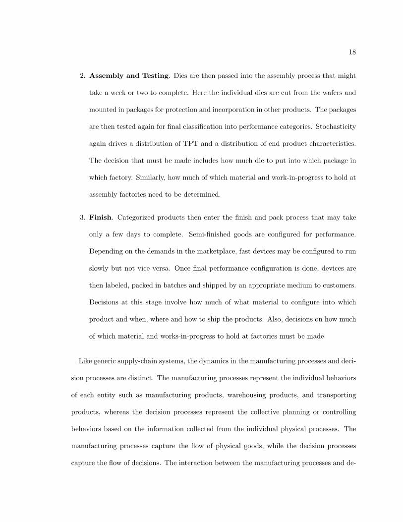
18
2. Assembly and Testing. Dies are then passed into the assembly process that might
take a week or two to complete. Here the individual dies are cut from the wafers and
mounted in packages for protection and incorporation in other products. The packages
are then tested again for final classification into performance categories. Stochasticity
again drives a distribution of TPT and a distribution of end product characteristics.
The decision that must be made includes how much die to put into which package in
which factory. Similarly, how much of which material and work-in-progress to hold at
assembly factories need to be determined.
3. Finish. Categorized products then enter the finish and pack process that may take
only a few days to complete. Semi-finished goods are configured for performance.
Depending on the demands in the marketplace, fast devices may be configured to run
slowly but not vice versa. Once final performance configuration is done, devices are
then labeled, packed in batches and shipped by an appropriate medium to customers.
Decisions at this stage involve how much of what material to configure into which
product and when, where and how to ship the products. Also, decisions on how much
of which material and works-in-progress to hold at factories must be made.
Like generic supply-chain systems, the dynamics in the manufacturing processes and deci-
sion processes are distinct. The manufacturing processes represent the individual behaviors
of each entity such as manufacturing products, warehousing products, and transporting
products, whereas the decision processes represent the collective planning or controlling
behaviors based on the information collected from the individual physical processes. The
manufacturing processes capture the flow of physical goods, while the decision processes
capture the flow of decisions. The interaction between the manufacturing processes and de-
19
cision processes captures the flow of financial and information data. The decision processes
quantitatively affect the manufacturing processes.
We have chosen a semiconductor manufacturing supply chain as our research domain to
study the multi-formalism modeling and simulation approaches for supply chain manage-
ment. The fast changing market and the continuous price declines require the semiconductor
manufacturer to decrease production lead-time while keeping the costs low. Furthermore,
the large variety of production cycles, uncertainty of customer demands, and the worldwide
distribution of manufacturing sites make it increasingly difficult to control the entire manu-
facturing process. A sound advanced decision process is necessary to unify the manufactur-
ing process and to reduce the planning cycle time. In consequence, it requires well-defined
simulation models to capture the practical behaviors of the real manufacturing processes
and feed the decision-making system with more accurate information.
2.3 Some Benchmark Problems in Semiconductor Manufacturing Supply Net-
work
The essential problem in semiconductor manufacturing supply network lies in multi-chain
and multi-product. A semiconductor manufacturing supply chain network can be described
in two parts: bill of material (BOM) which describes all the intermediate products that
need to be built to create a finished product, and topology that describes the physical layout
of the supply network in term of factories, warehouses, transportations and customers. The
BOM and topology together provide interrelated information to address the routines of the
products taken through supply chain network. The BOM provides the mapping of what
target products can be built from a set of source parts, whereas the topology configures the
connections of a set of entities at which a product may be determined to build, transport
or hold. In practice, there are a large number of entities and a large variety of products
20
involved in a real semiconductor manufacturing supply chain network. To simplify the
problem, a few of typical entities are chosen to construct the manufacturing supply chain
network while capturing as many of benchmark problems as possible (i.e., a basic network
structure as shown in Figure 1).
2.3.1 Bill of Material
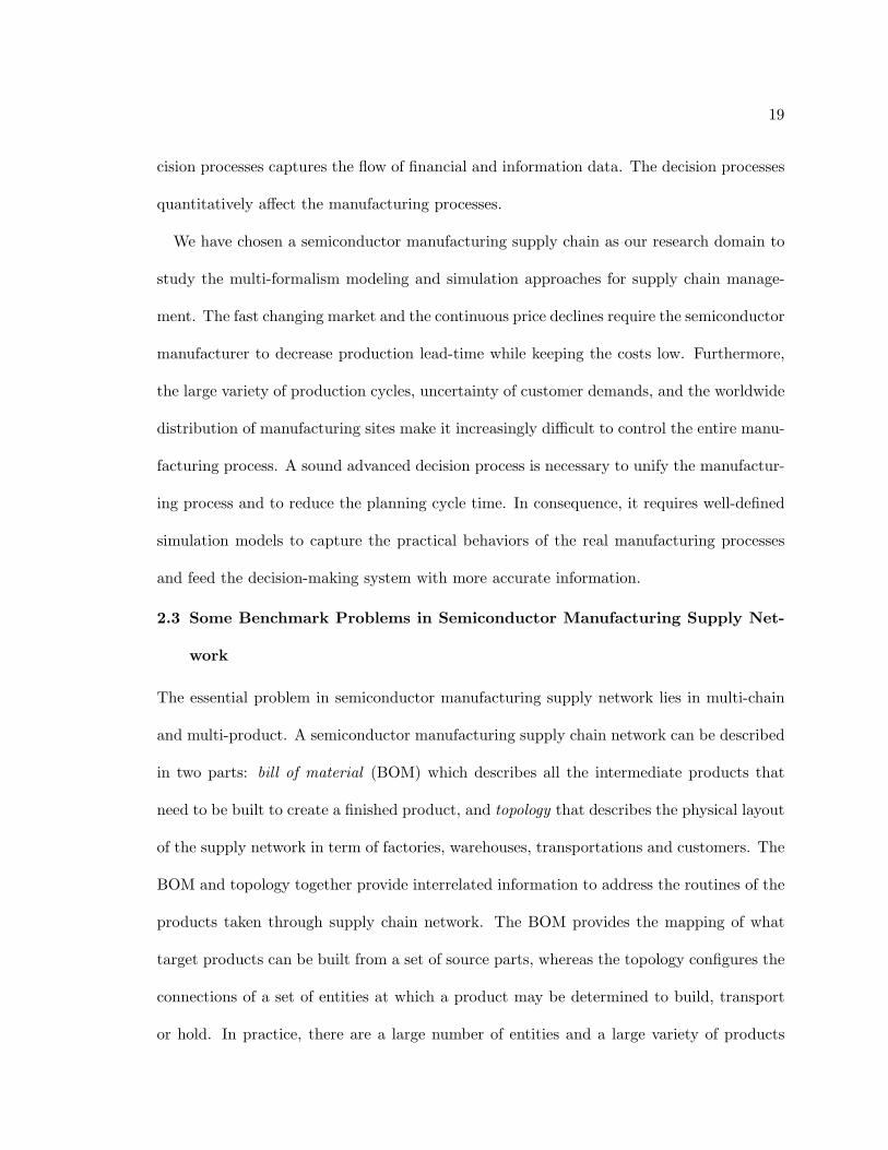
Figure 2 exhibits a BOM mapping from the source material at the left to the final products
at the right. That is, the product at the right is built from the products at the left. At the
right end, these are finished products ready for the customers.
Fig. 2. A Sample of Semiconductor Supply-Chain BOM Mapping
As show in the Figure 2, part of BOM mapping is determined by the decision process.
For example, it is the decision process to determine how much raw silicon will be released
for fabrication, based on the consideration of many factors such as customer demands fore-
casting, facility capacities, and the average production cycle time, etc. Part of the mapping
is built upon different types of manufacturing operations with stochasticity. For example,
21
the stochasticity in the assembly/testing process drives a distribution of productions with
different performance characteristics (i.e., high speed microprocessor vs. low speed micro-
processors), which is called split operation. Symmetrically, there is another operation called
assembly which represents that two or more product parts are assembled into one product,
such as assembling one package with one die in the assembly process. The split operation
is a characterization of a factory itself, whereas the assembly operation is often controlled
by the decision process. Another specialty shown in the BOM mapping is that multiple
splits of multiple distributions can result in different production flow giving the same end
products. That is, lower performance devices can be replaced by configuring higher perfor-
mance devices but cannot be the opposite (i.e., PkgA spd1 can be used to make product
ProdB server m-spd in Figure 2). Therefore, some fast devices can be transferred as slow
devices to meet specific customer demands.
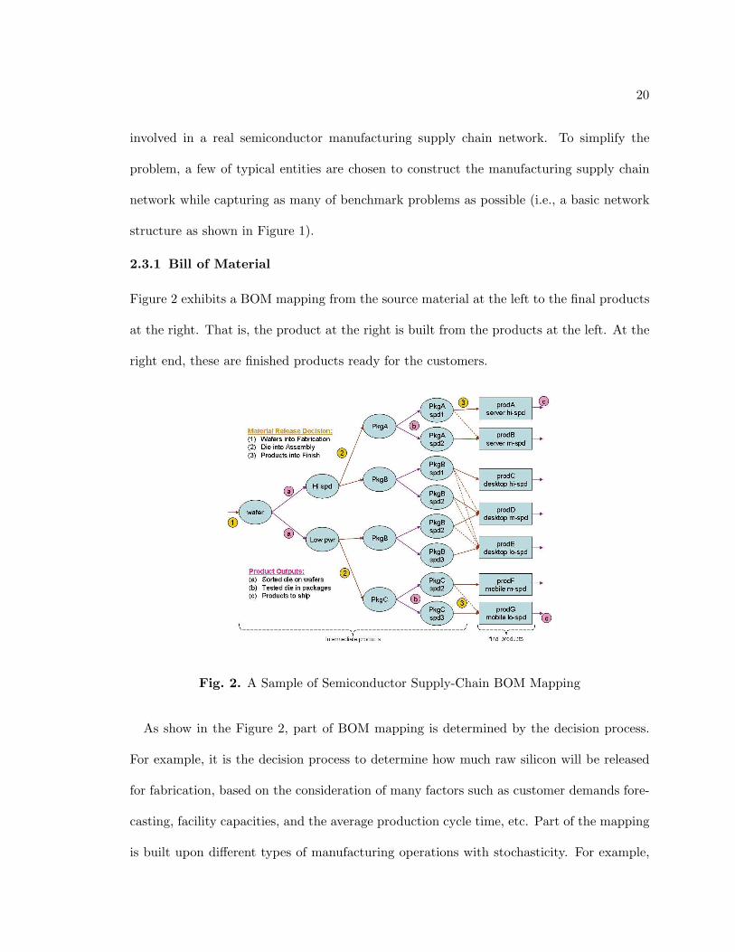
2.3.2 Topology
Figure 3 shows a sample of facilities topology in semiconductor manufacturing supply chain
network. It exhibits the distinguishing features in semiconductor manufacturing, such as
collecting parts from different inventories for assembly operation, stochastic splitting op-
eration inside one factory to produce products of different characteristics, cross shipping
between inventories, and supporting customer demands for multiple products, etc. The
configuration of BOM onto the topology is also presented in the figure, which depicts the
dependencies between the BOM and the supply network topology. That is, the connec-
tions between the facilities reflect the physical product flows taken through the BOM; the
characteristics of the manufacturing process described in the BOM are mapped onto the
properties of the individual facilities in the topology; and the decisions relied on in the
22
BOM are mapped onto the control inputs to the network facilities from some independent
planning and controlling system, which is different from the physical product flows.
Fig. 3. A Sample of Semiconductor Supply-Chain Topology
The semiconductor supply chain involves in different network topologies, diverse products,
and different types of flows across the entire system. A sound strategic planning and tactical
execution control for the factories, warehouses and transport links, is necessary to improve
the whole manufacturing supply chain system, while the modeling approach for the whole
manufacturing process should be configurable, scalable and flexible to support different
practical scenarios, and to analyze and evaluate the planning and controlling management.
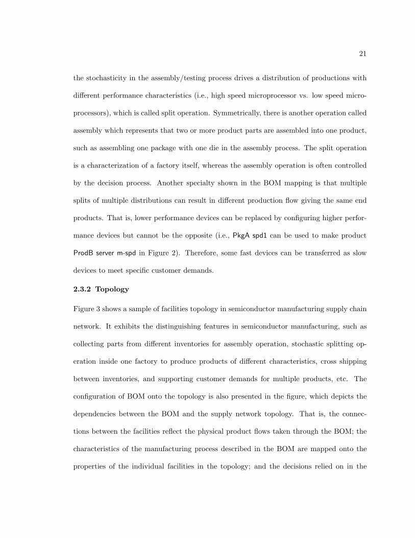
2.3.3 Domain View of a Semiconductor Manufacturing Supply-Chain System
As described in the previous sections, the semiconductor manufacturing supply chain system
domain can be considered to have two types of sub-systems—Process and Decision. The
Process sub-system represents the practical manufacturing processes, whereas the Decision
sub-system specifies the planning and/or control policies; they must work interdependently
to tackle practical system problems. Given the distinct functionalities and flow representa-
23
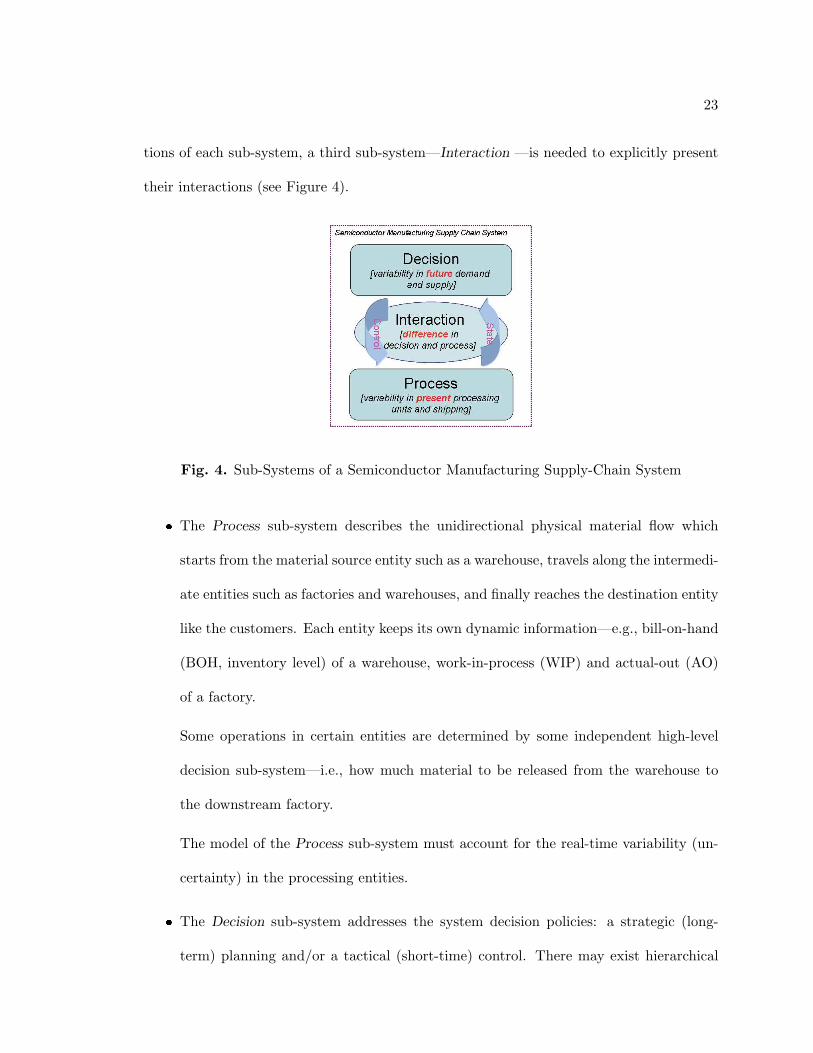
tions of each sub-system, a third sub-system—Interaction —is needed to explicitly present
their interactions (see Figure 4).
Fig. 4. Sub-Systems of a Semiconductor Manufacturing Supply-Chain System
� The Process sub-system describes the unidirectional physical material flow which
starts from the material source entity such as a warehouse, travels along the intermedi-
ate entities such as factories and warehouses, and finally reaches the destination entity
like the customers. Each entity keeps its own dynamic information—e.g., bill-on-hand
(BOH, inventory level) of a warehouse, work-in-process (WIP) and actual-out (AO)
of a factory.
Some operations in certain entities are determined by some independent high-level
decision sub-system—i.e., how much material to be released from the warehouse to
the downstream factory.
The model of the Process sub-system must account for the real-time variability (un-
certainty) in the processing entities.
� The Decision sub-system addresses the system decision policies: a strategic (long-
term) planning and/or a tactical (short-time) control. There may exist hierarchical
24
multiple decision sub-systems coordinating to manipulate the overall semiconductor
manufacturing supply chain system. In general the decision can be categorized as
strategic planning and tactical control. The former addresses a long-term strategy
whereas the latter describes short-time tactics.
The decisions are generally computed based on a set of entity dynamic information
which is provided by the processing entities in the Process sub-system and/or a set
of target references supplied by a higher level of decision sub-system.
The model of the Decision sub-system must account for the future variability in de-
mand and supply.
� The Interaction sub-system explicitly describes the exchange of system dynamic in-
formation and command control between the Process and the Decision sub-systems.
For some information, the exchange is straightforward between the two sub-systems.
But in most cases, aggregation/disaggregation calculation may be needed for the in-
formation exchange. For example, if a strategic planning needs an average inventory
levels of a warehouse for certain past time segment and its start commands to the
factories are for certain future time period, the operations of aggregation and disag-
gregation are needed, since the Process sub-system generally provides a set of basic
dynamic states at the current time. Although such operations could be calculated
inside the Process or the Decision sub-system, the close coupling of the interaction
with a specific functional sub-system results in less modularity and less flexibility. An
independent interaction sub-system is desired to separate the interaction activities
from the functional activities of a specific sub-system.
25
The model of the Interaction sub-system must account for the differences between the
Process and Decision sub-systems.
2.4 Modeling and Simulation Technologies Used in Supply-Chain Systems
Supply chain management is the combination of art and science that goes into improving
the way for a company to finding the raw materials it needs to make products, manufac-
turing those products, and delivering the products to customers. According to SCOR [82],
there are 5 basic management processes in a supply chain network: (1) Plan—a strategic
process of supply chain management that manages all the resources that go towards meet-
ing customer demands while keeping maximal profits, (2) Source—a supply management
process that chooses the suppliers, develops a set of pricing, delivery and payment pro-
cesses with suppliers, and creates metrics for improving and managing the relationships,
(3) Make—a manufacturing management process that schedule activities for productions,
testing, packaging, and preparation for delivery, (4) Deliver—a logistics management pro-
cess that coordinates the receipt of orders from customers, develops a network of warehouses,
transports products to customers, and sets up invoicing systems to receive payments, and
(5) Return—a problem-handling process that manages returns of raw materials and returns
of products from customers. Each of the five basic management processes comprise many
specific tasks. Although IT technology has been widely used in supply chain management,
no IT technology exists that can handle all the tasks in one software application. The ex-
isting supply chain management software tackles only specific problems. Two main types of
supply chain software are (I) supply chain planning software, which often uses mathematical
algorithms to help improve the flow and efficiency of the supply chain and reduce inventory,
and (II) supply chain execution software, which helps execute supply chain manufacturing
steps.
26
There are some large vendors who have been attempting to assemble many of the different
chunks of software into a single package to facilitate the enterprise business process. For
example, as a supply chain company, i2 [35] has provided different products to optimize and
manage major business processes along a supply chain such as Supply Chain Planner, Fac-
tory Planner, and Transportation Optimizer. It is now integrating these products through
a middleware integration service to construct an agile business platform—a service-oriented
architecture which integrates different services and supports external coordination as well.
In this service-oriented business platform, different services from i2 and third-parties can
be ‘plugged in’ and finally implemented as the next generation of supply chain management
solutions. As part of Oracle E-Business Suite, the Oracle Supply Chain Planning product
family [64] is another example of group software supporting holistic planning from long-
term planning (e.g., advanced supply chain planning and demand planning) to short-term
scheduling (e.g. manufacturing scheduling). Another SCM group software is mySAP SCM
[75] produced by SAP. It enables adaptive supply chain networks by providing not only
planning and execution capabilities to manage enterprise operations, but also visibility, col-
laboration and radio frequency identification (RFID) technology to streamline and extend
those operations beyond corporate boundaries.
Some commonalities of the SCM group software is that (i) they all provide different
types/levels of planning/optimization software modeling for major supply chain business
processes, (ii) an integration platform is supported among the software models, and (iii)
they can collaborate with other software such as ERP (Enterprise Resource Planning) soft-
ware and supply chain execution software directly for real-time supply chain management.
However, these platforms are limited in that very few simulation technologies exist in the
planning/optimization software models that analyze/verify the designed plans before they

27
are really applied into supply chain network. Although the integration platform is sup-
ported, each planning model is developed relatively independently. Models/platforms are
not equipped to simultaneously consider the information provided by other software mod-
els. Much needs to be done to coordinate different levels of planning and control to develop
truly integrated management software for the holistic supply-chain systems.
CHAPTER 3
SEMICONDUCTOR SUPPLY-CHAIN MODELING AND SIMULATION AP-
PROACHES
Different modeling approaches have been proposed to specify the dynamic behaviors in semi-
conductor manufacturing supply chain systems for the purpose of tackling specific system
problems. The researches on computer-aided supply chain management can be categorized
as control-theoretic paradigm, operations research methods, and simulation approaches1.
Control theory makes an analogy between supply chain network and the control systems.
Therefore, some advanced controlling technologies can be used for supply chain manage-
ment. Operations research methods include optimization programming (i.e., linear pro-
gramming), statistical analysis and business games, etc. They are generally used to design
advanced planning systems to achieve some specific objectives along the supply chain. The
simulation approach is to develop an executable system model to evaluate the actual system
dynamics by applying the previous controlling/planning approaches. Simulation approach
by itself cannot provide supply chain management; it must integrate at least one of the
previous controlling/planning models.
3.1 Process-Oriented Modeling and Simulation
3.1.1 System-Theoretic Discrete-Event Simulation
Discrete Event Simulation (DES) has been generally considered suitable for modeling and
simulating the manufacturing behaviors in the semiconductor supply chain. It can describe
time uncertainty (e.g., customer demands may arrive at some random intervals). It can
include stochastic elements. It can track the different types of flow information at differ-
ent levels of abstraction, such as at a factory level or a machine level. More importantly,
it can handle unexpected events. These specialties cannot be easily represented in other
1Given different perspectives of the supply chain management, there exit different waysfor categorizing supply chain modeling and analysis approaches [57, 39, 71]
29
system mathematical models. Therefore, DES can be used to model the most complex
behavior in manufacturing supply-chain network. Specifically, Discrete EVent System spec-
ification (DEVS) [104] is a mathematical modeling formalism for describing (discrete and
continuous) dynamical systems as discrete event models. The formalism, based on generic
system-theoretic concepts, supports developing models with well-defined behaviors. It uses
mathematical set theory and provides a framework for system modeling and simulation.
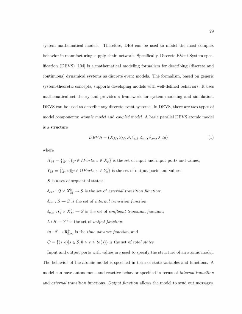
DEVS can be used to describe any discrete event systems. In DEVS, there are two types of
model components: atomic model and coupled model. A basic parallel DEVS atomic model
is a structure
DEV S = (XM , YM , S, δext, δint, δcon, λ, ta) (1)
where
XM = {(p, v)|p ∈ IPorts, v ∈ Xp} is the set of input and input ports and values;
YM = {(p, v)|p ∈ OPorts, v ∈ Yp} is the set of output ports and values;
S is a set of sequential states;
δext : Q×XbM → S is the set of external transition function;
δint : S → S is the set of internal transition function;
δcon : Q×XbM → S is the set of confluent transition function;
λ : S → Y b is the set of output function;
ta : S → <+0,∞ is the time advance function, and
Q = {(s, e)|s ∈ S, 0 ≤ e ≤ ta(s)} is the set of total states
Input and output ports with values are used to specify the structure of an atomic model.
The behavior of the atomic model is specified in term of state variables and functions. A
model can have autonomous and reactive behavior specified in terms of internal transition
and external transition functions. Output function allows the model to send out messages.
30
Time advance function captures timing of models. Confluent function can be used for
modeling simultaneous internal events and external events.
A coupled model is composed of one or more atomic models or coupled models. The
structure specification of a coupled model includes input & output ports, a set of compo-
nents, and component coupling information. The coupling information is categorized as (1)
the external input coupling (EIC) - coupling of coupled model input ports to input ports
of some component, (2) the external output coupling (EOC) - coupling of component output
ports to the coupled model output ports, and (3) the internal coupling (IC) - coupling of
component output ports to input ports of components. A coupled model doesn’t have direct
behaviors. Its behavior is based on the message exchanges between itself and its components
as well as message exchanges among the components, through coupling connections. The
coupling provides interaction between components. DEVS enjoys the property of closed
under coupling. That is, every coupled model can be reduced to an atomic model with
identical behavior as the coupled model. This property supports modeling larger models in
a hierarchical manner.
Comparing the ad-hoc event-queue controlling mechanism, DEVS simulation protocol
provides a well-defined framework to execute the dynamic behaviors of DEVS models, in
which timing and causality is well controlled. Each atomic model has a corresponding
simulator, while each coupled model has a corresponding coordinator. A root coordinator is
defined to coordinate the simulators and coordinators by executing the simulation algorithm,
invoking the appropriate functions and advancing simulation time properly. The simulation
engine structure is shown in Figures 5.
The simulation algorithm [104] can be described as followed:
1. Coordinator sends nextTN message to request for each of the simulators
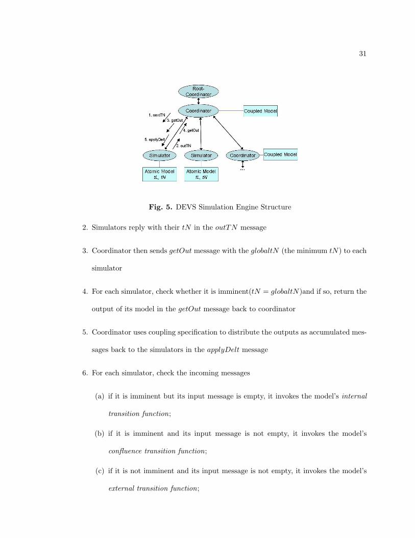
31
Fig. 5. DEVS Simulation Engine Structure
2. Simulators reply with their tN in the outTN message
3. Coordinator then sends getOut message with the globaltN (the minimum tN) to each
simulator
4. For each simulator, check whether it is imminent(tN = globaltN)and if so, return the
output of its model in the getOut message back to coordinator
5. Coordinator uses coupling specification to distribute the outputs as accumulated mes-
sages back to the simulators in the applyDelt message
6. For each simulator, check the incoming messages
(a) if it is imminent but its input message is empty, it invokes the model’s internal
transition function;
(b) if it is imminent and its input message is not empty, it invokes the model’s
confluence transition function;
(c) if it is not imminent and its input message is not empty, it invokes the model’s
external transition function;
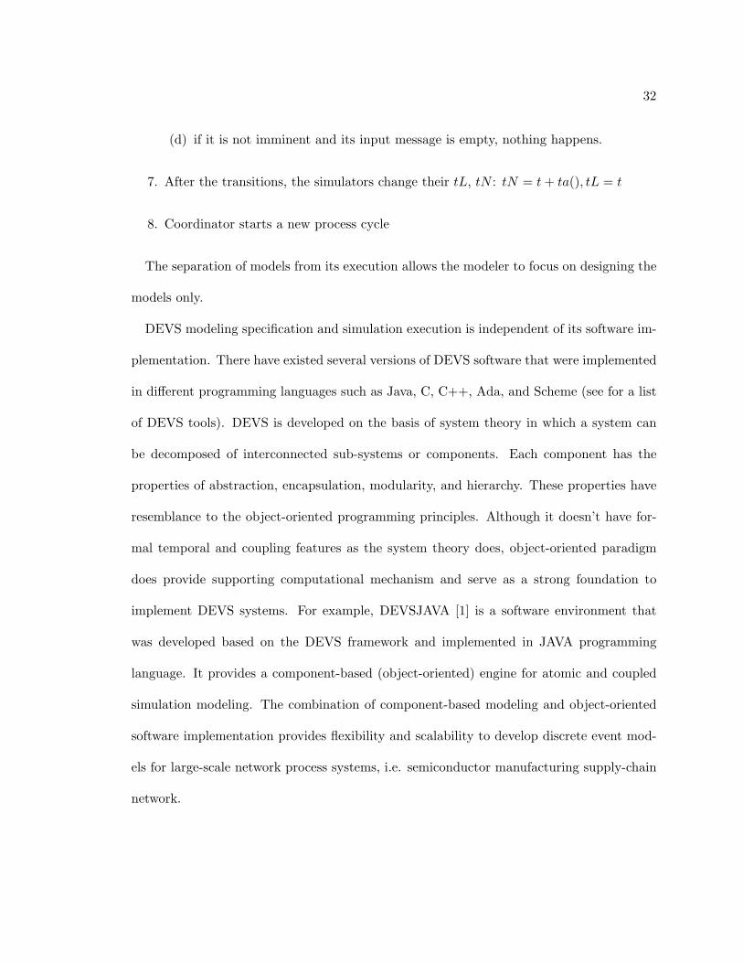
32
(d) if it is not imminent and its input message is empty, nothing happens.
7. After the transitions, the simulators change their tL, tN : tN = t + ta(), tL = t
8. Coordinator starts a new process cycle
The separation of models from its execution allows the modeler to focus on designing the
models only.
DEVS modeling specification and simulation execution is independent of its software im-
plementation. There have existed several versions of DEVS software that were implemented
in different programming languages such as Java, C, C++, Ada, and Scheme (see for a list
of DEVS tools). DEVS is developed on the basis of system theory in which a system can
be decomposed of interconnected sub-systems or components. Each component has the
properties of abstraction, encapsulation, modularity, and hierarchy. These properties have
resemblance to the object-oriented programming principles. Although it doesn’t have for-
mal temporal and coupling features as the system theory does, object-oriented paradigm
does provide supporting computational mechanism and serve as a strong foundation to
implement DEVS systems. For example, DEVSJAVA [1] is a software environment that
was developed based on the DEVS framework and implemented in JAVA programming
language. It provides a component-based (object-oriented) engine for atomic and coupled
simulation modeling. The combination of component-based modeling and object-oriented
software implementation provides flexibility and scalability to develop discrete event mod-
els for large-scale network process systems, i.e. semiconductor manufacturing supply-chain
network.
33
3.1.2 Agent-Based Modeling
Agent-based approach is suitable for studying systems which consist of multiple autonomous
or semi-autonomous components that are distributed and interact with each other through
message passing. The agent components generally have built-in behavioral rules and may
learn to improve performance over time. Supply chain system are a typical example, since
the manufacturers, warehouses, distributors, customers and the decision makers can be con-
sidered as constituent agents, each of which is in charge of its own responsibilities and loosely
coupled with others to work together to solve problems that are beyond individual capabil-
ity or knowledge, under the unpredictable conditions. There have existed some researches
concentrating on multi-agent approach for modeling supply chain dynamics [22, 74, 85]. For
example, in [85] different types of agents are specified to represent structural elements (e.g.
production agent and transportation agents) and control element (e.g. demand control and
supply control) in the supply chain domain. The agents were defined by a set of attributes
(describing its own state), knowledge of some other agents, a set of interaction constraints,
a set of incoming and outgoing messages, a set of control policies available, and a set of
function rules to handle incoming messages based on domain knowledge, current state and
control policies. These agents were in fact specified in term of software components. This is
considered as a disadvantage of agent-based approach due to the lack of universally accepted
theory so far for specifying agent structures and dynamics. Given the level of requirements,
the agent model could be simple or could be very complex.
Agent-based modeling approach and realization doesn’t have well-defined timing concepts
which is key in the simulation. Therefore, it cannot very well support partial time ordering,
simultaneous multiple event handling, and processing events in zero logical time. Lack of
such capabilities makes it difficult to specify varying levels of complex dynamics of discrete
34
processes. In addition, it can also limit the interactions with other types of models (e.g.,
model-based controller or optimization) where time-based synchronization is key.
3.2 Strategic Planning and Tactical Control
3.2.1 Operations Research Approach—Linear Programming for Optimization
Operations research has contributed to models building and solving by using mathematical
methods to coordinate the flows along supply chains. Typically among them are Linear and
Mixed Integer Programming, Constraint Programming, and Generic Algorithms. The exis-
tence of powerful solution algorithm and respective standard software for solving LP models
(e.g., CPLEX in ILOG OPL Studio [36]) makes LP one of the most famous optimization
techniques in decision situations where LP models can handle thousands of variables and
constraints within a few minutes on a personal computer.
The general form for a LP problem is described as follows [70].
min /max f(X1, X2, . . . , Xn) := c1X1 + c2X2 + . . . + cnXn (a)
ai1X1 + ai2X2 + . . . + ainXn
≤
=
≥
bi, i = 1, . . . , m (b)
(Xj ≥ 0) ∨ (Xj ≤ 0) ∨ (Xjurs), j = 1, . . . , n (c)
(2)
Where X1, X2, . . . , Xn represent decision variables and “urs” indicates unrestricted in sign.
Here (a) is Objective Function, (b) is Technological Constraints, and (c) is Signed Restric-
tions.
The different decision variables are assumed to correspond to various activities from
which any solution will be eventually synthesized, and the values assigned to the variables
by any given solution indicate the activity levels in a considered plan. Each technological
35
constraint in Equation 2 is assumed to impose some restrictions on the consumption of a
particular resource.
Solution algorithms (named Solver) are necessary to execute LP models. Solving a LP
model can be hard and time-consuming when the model involves a large number of vari-
ables and constraints. Very powerful solution algorithms and respective standard software
have been developed to solve LP models. For example, CPLEX from ILOG OPL Stu-
dio has provided modeling syntax for modeling mathematical optimization problems in a
straightforward way. It also supports fast and reliable execution of fundamental algorithms
for solving LP problems. Some other LP solver software includes MATLAB Optimization
Toolbox [47], XPRESS-MP suite [9], etc.
As in the semiconductor supply chain systems, Linear Programming optimization has
been used to formulate strategic planning problems for allocating capacity to satisfy cus-
tomer demands while minimizing costs and maximizing profits. For example, in [38] the
core formulation of LP is based on mass balance and capacity constraints and an objec-
tive function that includes minimizing costs and maximizing revenues. To describe a single
material flow leading to “ProdA in Figure 2 with the only top-most facilities—Fab/Test1,
Die1, Assembly/Test1, SFGI1, Finish1, CW1 and Ship1 (see Figure 3), a simple example
formulation was specified. The input variables which are used for specifying the constraints
include demand forecasts, inventory targets, factory capacity, yield and TPT, initial factory
WIP, and initial warehouse inventory. The corresponding financial model variables (e.g.,
manufacturing costs, inventory holding costs, penalty for missing inventory targets and de-
mands, and selling prices) can also be included. The decision variables are material release
plan for all manufacturing facilities. Also available in the decision output is a transporta-
tion plan, an inventory plan including inventory levels relative to the specified targets, and
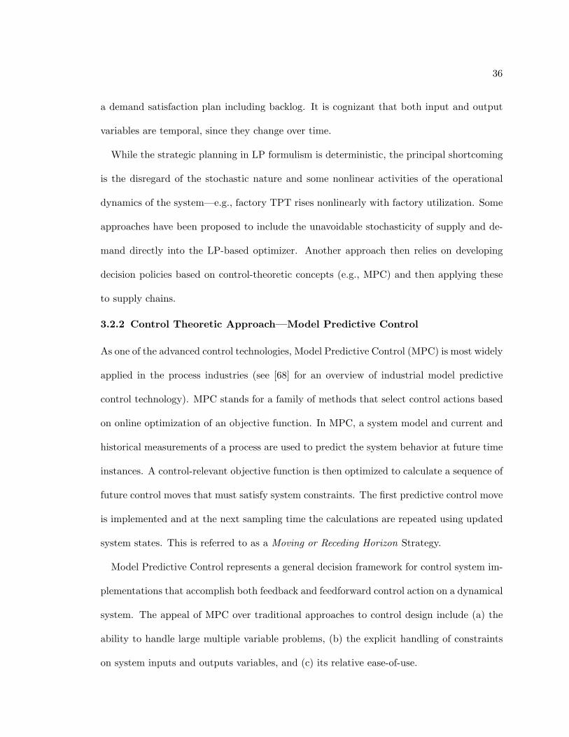
36
a demand satisfaction plan including backlog. It is cognizant that both input and output
variables are temporal, since they change over time.
While the strategic planning in LP formulism is deterministic, the principal shortcoming
is the disregard of the stochastic nature and some nonlinear activities of the operational
dynamics of the system—e.g., factory TPT rises nonlinearly with factory utilization. Some
approaches have been proposed to include the unavoidable stochasticity of supply and de-
mand directly into the LP-based optimizer. Another approach then relies on developing
decision policies based on control-theoretic concepts (e.g., MPC) and then applying these
to supply chains.
3.2.2 Control Theoretic Approach—Model Predictive Control
As one of the advanced control technologies, Model Predictive Control (MPC) is most widely
applied in the process industries (see [68] for an overview of industrial model predictive
control technology). MPC stands for a family of methods that select control actions based
on online optimization of an objective function. In MPC, a system model and current and
historical measurements of a process are used to predict the system behavior at future time
instances. A control-relevant objective function is then optimized to calculate a sequence of
future control moves that must satisfy system constraints. The first predictive control move
is implemented and at the next sampling time the calculations are repeated using updated
system states. This is referred to as a Moving or Receding Horizon Strategy.
Model Predictive Control represents a general decision framework for control system im-
plementations that accomplish both feedback and feedforward control action on a dynamical
system. The appeal of MPC over traditional approaches to control design include (a) the
ability to handle large multiple variable problems, (b) the explicit handling of constraints
on system inputs and outputs variables, and (c) its relative ease-of-use.

37
A MPC model consists of a System Prediction Model and an Optimizer. System predic-
tion model is generally described in term of linear time-invariant state space model (See
Equation 3).
Xk+1 = AXk + BuUk + BvDk
Yk+1 = CXk
(3)
where Uk ∈ <mu is a vector of input (or manipulated) variables, Xk ∈ <mx is a vector of
state variabels, Yk ∈ <my us a vector of output (or controlled) variables, and Dk ∈ <mv is
a vector of disturbance variables.
The procedure of how a MPC controller controls a system is informally described as
follows (see Figure 6):
1. Update: the system under control sends MPC the latest outputs (controlled variables).
2. Estimate: estimation is calculated based on the previous and current states and out-
puts, the previous inputs, and some anticipated measured disturbance.
3. Optimize: the estimated output trajectories and its reference trajectories for some
future time horizon (called Prediction Horizon p) are then sent to the optimizer which
has defined some objective functions and constraints.
4. Control: the solution of optimization is some future movements (called Move Horizon
m) of the manipulated variables. The current move is used as a feedback to the
controlled real system or simulation system.
The procedure is repeated once the new information is available from the system.
It has been shown in [96] that MPC can be used effectively as a tactical controller for
high volume semiconductor supply chain systems to handle nonlinear, stochastic dynamics
38
Fig. 6. MPC Structure
and unpredictable demand changes while enforcing constraints on desired inventory lev-
els and production and transportation capacities. In the system prediction model, which
is a simplified system as compared with the real system or a detailed simulation model,
the controller uses the previous information on warehouse inventories, actual customer de-
mands, factory starts, future information on inventory targets, and forecasting customer
demands to estimate future inventory levels. In the optimizer, a sequence of future factory
starts is calculated by solving the optimization whose objective functions include keeping
inventory levels close to targets, minimizing changes in the manipulated factory starts, and
maintaining the factories starts at strategic planning targets.
3.2.3 Other Approaches
There exist other approaches that have been widely used for supply chain system modeling
and analysis. Spreadsheets, System Dynamics, and Business games are among them.
Spreadsheet software has made corporate modeling very popular, given its simplicity, in-
tuitionism of use, powerful functions for sophisticated computations, and excellent graphic
39
displays. It has been especially widely used by business users such as managers. More
features and introduction can be found in [83] regarding the spreadsheet simulation. The
disadvantages of spreadsheet modeling are also obvious. It can only handle a limited num-
ber of variables, have limited storage space, and can become very complex when many
interdependent relations need to be modeled.
System dynamics (SD), originally known as Industrial Dynamics, was developed by For-
rester [16]. The SD methodology is essentially using information feedback and delays to
understand the dynamic behavior of complex systems. In the original “Forrester model”—a
4-link production-distribution system consisting of retailer, wholesaler, distributor, and fac-
tory, 6 types of system flows were described, namely the flows of information, materials,
orders, money, manpower, and capital equipment. Based on development and use of the
SD simulation model and results analysis, Forrester pointed out some issues evolving in
supply chain management, such as demands amplification and inventory swings, which are
still current research issues. There has been much research using SD for supply chain man-
agement [3]. The disadvantages of SD methodology include the lack of sensitivity analysis
and the limited simulation capability in comparison with other sophisticated discrete event
simulation packages available today.
Business or management game is an interactive simulation that provides a simulated
‘world’ of SC environment for managers themselves to operate. Games may be used for
both education and research purposes. Two subtypes of games are distinguished in [40]:
strategic games in which several teams of players who represent companies that compete
with each other in the simulation world, and operational games where a single team of one
or more players interact with the simulation model.
40
In some existing researches, multi-modeling approaches has been proposed for integrated
supply chain management modeling, simulation and analysis [23, 42, 91, 101]. High abstract
level of coordination mechanism between different modeling approaches must be considered
to achieve a systematic integration.
3.3 Modeling and Simulation Environments
The modeling and simulation approaches mentioned above is independent of the imple-
mented software. There have existed some commercial software tools to support develop-
ment and simulation of different models (e.g., MatLab, SimuLink, and Arena [73]). In the
academic world, some generic simulation tools are implemented for the research on sup-
ply chain management. Among them are DEVSJAVA, Chi [31], etc. Each software tool
provides unique capabilities to solve specific problems. No tool with a rigorous modeling
and simulation foundations exist to support heterogeneous modeling and simulation for
manufacturing supply chain systems ([10, 59, 76]).
Supply chain is a large-scale network system that crosses multiple business entities some
of which are inside an organization, while some are outside the organization. These business
entities operate independently while interact with each other at the same time. It may refer
to a distributed computing environment. The advantages of distributed simulation of supply
chain network include (1) utilizing additional computing power, specific operating systems
or peripheral devices, (2) simulating simultaneous processes in different locations, and (3)
easily replacing one model (e.g. behavior simulation model or decision control model) with
other models. However, construction of the distributed simulation environment for supply
chain systems is still an open research question. Specifically, there is no software to support
the distributed simulation of multi-formalism supply chain models yet.
41
3.4 Summary
Different modeling approaches are described in term of characteristics as well as specialties
for solving specific supply chain problems. In comparison with operations research methods
and control-theoretic approach, simulation approach such as discrete-event modeling can
represent more realistic system dynamics since it can account for stochasticity and other
practical complex behaviors. Simulation approach by itself is not suitable for providing a
planning/control for the supply chain system. But it is suitable to be used for analyzing and
evaluating how well a specific planning/control model is designed for a supply chain system.
The mathematical methods of operations research (OR) such as LP can support advanced
planning process via solving optimal problems. But the system dynamics expressed in LP is
usually simplified; it is very difficult to deal with uncertainty. Control-theoretic approaches
such as MPC are proposed for supply chain tactical control on the basis of its analogy to
process control system, as it offers a combined feedback and feedforward decision framework
and provides stochastic control and multiple variable control in addition to the optimal
techniques. However, the system dynamics modeled in MPC is also simplified and it may
not be suitable for long-term strategic planning. In a short, different modeling approaches
are fundamentally distinguished and focus on specific supply chain problems, although they
are representing the same supply chain system. The different classes of modeling approaches
are complementary to solve realistic supply chain management problems.
CHAPTER 4
MULTIFACETED MODEL COMPOSITION AND DISTRIBUTED SIMULA-
TION
It has been shown that a monolithic modeling approach is not suitable for studying the
supply chain management. Although much research has been focusing on individual ap-
proaches, there has been much less research on separation of the system simulation modeling
from the planning/control modeling and integration of the multiple modeling approaches in
a heterogeneous or specifically distributed environment. The integration of multiple model-
ing approaches can be specified at the different levels of abstraction. Integration of models
could be via low-level programming, high-level interoperability techniques, or multi-model
composability approaches. It has been proved that it is a not trivial problem to have two
dissimilar modeling formalisms tied together.
Different levels of model composition definition have appeared in the modeling and simu-
lation research literature [11, 10, 65]. The multi-level concept is similar to the level concept
in OSI network models. In this chapter, the modeling composition concepts and approaches
from different perspectives are discussed.
4.1 Modeling Formalism Composition Concepts and Approaches
A modeling formalism can be defined to consist of two parts—model specification and exe-
cution algorithm [80]. For large systems such as semiconductor manufacturing supply-chain
systems which are considered to have parts of dynamics that are intrinsically different, it
is crucial to use multiple modeling formalisms. Approaches of composing different mod-
eling formalisms are different. Most Recently the modeling composition approaches are
classified into mono, super, meta, and poly modeling composition, each of which provides
different kinds of capabilities toward model composition [81]. The formal two approaches
are grounded in the concept that in principle a single formalism can be well suited for mod-
43
eling different part of a system in certain cases. In contrast, the latter two are aimed at
some other cased where disparate modeling formalisms are crucial to describe the parts of
a complex system. It is important that each approach must ensure the interactions among
composed models are structurally and behaviorally well defined despite the difference among
the composition approaches.
A modeling formalism typically has both syntactic and semantic parts. The syntactic part
specifies the elements (and their relationships) of valid models whereas the semantic part
pertains to the meaning of the models. The meaning of the model can be expressed in an op-
erational fashion by explicitly describing how the model can be executed/simulated/solved.
The operation approach is essentially transforming the model to a behavior trace appropri-
ate state trajectories. In the case of expressing a system with multi-formalism components,
the high-level composite meaning of the system may have to be studied in conjunction with
some lower levels details for which different formalisms are most suited.
4.1.1 Mono- and Super-Formalism Modeling
In the mono modeling, a single modeling formalism is used. The key advantage of using
mono approach is that decomposition (or hierarchically composition) of a system model into
(from) parts can be carried out in a systematic way (e.g., in [98]). one execution protocol is
used for the composite model execution. This approach significantly simplified integration
of models and their executions. However, use of the mono modeling approach may not be
suitable when the system parts (e.g., manufacturing process dynamics vs. tactical control
in semiconductor manufacturing supply-chain systems) to be modeled are distinct—the
models are best described in different modeling paradigms.
The super-formalism modeling refers to a modeling formalism (framework) within which
two or more fundamentally distinct model types can be encapsulated. A general encapsu-
44
lation approach is to use different levels of abstractions of multiple models and hide the
details of an encapsulated model specification inside the enclosing model specification. In
this approach, the super formalism must assert that the kinds of disparate dynamics of
the enclosed modeling formalism can be specified within it. Therefore, such model encap-
sulation requires the enclosed model to be well defined—the input and output structure
and the encapsulation behavior—through the enclosing model specification. For example, a
simplified optimization model described in LP can be encapsulated as an I/O system—i.e.,
an atomic DEVS component. Certain details of the enclosed model specification may have
to be hidden to ensure model interactions.
In addition, there exist a strong form of super-formalism modeling in which the com-
position of different kinds of model specifications is specified at the level of state-based
specification rather than at the input/output [81]. For example, a coupled multi-formalism
specification was developed by Praehofer [66] as a basic system-theoretic formalism for
combined discrete/continuous modeling. This approach provides a theoretical framework
within which continuous, discrete-time and discrete-event models can be expressed. Some
subsequent research has focused on extending discrete event specification to represent con-
tinuous and discrete-time models (e.g., [41, 102]). The DEVS formalism was proposed to
support modeling combined DEVS&DESS models [105] without model transformation and
thus user-defined model encapsulation.
Another approach is Ptolemy [67] which supports modeling of mixed signal systems [13].
It formalizes input/output interactions among actors (model components) under the control
of directors.
In the super formalism modeling approach, the execution of the enclosing models and
those that are encapsulated are interoperated under the super formalism’s execution algo-
45
rithm. That is, the execution of the enclosed models are viewed as an atomic operation
within the super formalism execution algorithm.
4.1.2 Meta-Formalism Modeling
Meta-modeling is a process of modeling formalisms. In the meta modeling composition
approach, different types of model specifications are transformed or abstract to another
modeling formalism. The meta-formalism should provide abstract syntax such as denoting
entities of the model formalisms, their attributes, and relationships. Expressions of the
constraints is usually required when specifying the modeling formalism. The meta-formalism
must be capable of accounting for difference between disparate model specifications to be
composed.
A meta-modeling approach was proposed in [12] to allow for the specification of composite
systems consisting of heterogeneous components expressed in different formalisms. In this
approach, formalisms are meta-modeled and stored as graphs. A Formalism Transformation
Graph (FTG) is modeled as graph grammar, in which the transformation mappings between
two different formalisms are well-defined. The end goal of FTG is some common formalism
which can be transformed to programming code and simulated.
The main objective of meta-modeling is to support automated model transformation
instead of relying on ad-hoc and error prone means. It seeks to provide a means to view all
models of a system in a uniform setting by transforming disparate models into one common
representation.
In the meta modeling composition approach, the execution algorithms of the disparate
model specification are abstracted into model constructs and operations (e.g., a set of soft-
ware components, or a set of services as in HLA) that are intended for interoperating
46
different execution algorithms. Therefore, the model specification and execution algorithm
is weakly separated from one another [81].
4.1.3 Multi-Formalism Modeling
The multi-formalism modeling (or poly modeling) approach described here focuses on con-
structing modeling framework within which the interaction between disparate modeling
formalisms is explicitly handled. For example, the concept of Knowledge Interaction Bro-
ker was first proposed in [79] as the modeling interaction specification to compose an
iterative input/output observation formalism (system-theoretic modeling formalism) with
non-monotonic reasoning (artificial intelligence formalism). The modeling interaction spec-
ification is concerned with both modeling composability and execution interoperability.
The main difference between meta modeling composition and poly modeling composition
is that in the poly modeling composition approach, models are not transformed to a set of
models all of which are described in accordance to a single modeling formalism. Modeling
the interaction of the disparate models can support systematically composition of syntax
and semantics of the known modeling formalisms—it provides message mapping and rich
data transformation. The composition separates modeling composability from execution
protocol interoperability—the execution algorithm of the interaction model is explicitly
responsible for interoperability between the disparate models.
4.2 Software Component Specification and Interaction
The software engineering paradigm leans toward specifying a system in terms of semi-formal
modeling techniques and conceptual approaches. In the software paradigm, a system, which
is generally decomposed of sub-systems or components, is described in terms of various spec-
ifications within a single modeling framework. Such a framework is often generalized and
provides a variety of specifications (e.g., activity and statechart diagrams). There are no
47
common semantics specified among the specifications; therefore, it becomes necessary to
depend on weak specifications to characterize component models, or rely on ad-hoc low-
level programming using APIs. Unified Modeling Language (UML) [89] is being widely
used for describing software components as well as their interactions, whereas eXtensible
Markup Language (XML) [99] is used for information exchange among software compo-
nents. Furthermore, the software engineering community promotes platform-independent
business logic model development, which is then used to derive a platform-specific software
model and subsequently automatic generation of target application code (known as Model
Driven Architecture, MDA [51]). Two MDA specifications are Meta-Object Facility and
XML Metadata Interchange, which are important for ensuring different specifications to
work together using XML for information exchange between models and meta-models.
Software engineering approaches have been directly utilized for handling composite in-
teraction issues in systems with disparate model components. Besides the interface spec-
ification for component-based software composition, some research shows the necessities
of taking protocols (behavioral types) into component interaction specification to ensure
compatible interactions between software components (i.e., see [4, 42, 52]). These studies
indicate that the interface by itself lacks the expression of the context (e.g., pre-condition or
post-condition of running the interface methods) in which the interface methods can be in-
voked. Agent-based and actor-based modeling are the typical examples that use component-
based software approaches.
Agent-based modeling and simulation approaches can be considered as using component-
based software methodology, since there is no universally accepted theory of modeling agent
dynamics yet.
48
Ptolemy [67] can also be considered as a component-based software modeling environment
that supports hierarchically composing a variety of computation models. The theoretical
basis of the computational framework relies on token-based dataflow to combine execution
of models of mixed signal and hybrid systems. An independent Model of Control (MoC)
and its implementation (called domain) [45] is proposed to separate the flow of control
and data between components (called actors) from the actual functionality of individual
components, and to coordinate the execution of the composite components. This approach
can also be viewed as a type of multi-formalism but with a software engineering focus.
Component-based software development methodology can be useful for certain aspects
of constructing a systematic modeling composability framework.
4.3 Service-Oriented Interoperation
As noted earlier, a formalism is defined as a pair. The modeling composition approaches
in the previous section were described in term of model specifications. The separation of
model specification and execution protocol makes it possible to treat model composabil-
ity and execution interoperability differently given different composition approaches. The
dynamic behavior of each model in certain formalism is computed by its simulator/solver.
Interoperation refers to how different simulators/solvers interact with each other via some
middleware services. It resolves the composition of disparate model types in the trajec-
tory level. In this section, we will give a brief discussion on model interoperability from
simulation perspective and software component perspective as well.
The interactions between the models can be specified through interface or service specifi-
cations. In the light of service-oriented philosophy, interoperation enables different software
programs (simulators or executors) to exchange messages, in which some generic interop-
eration services are provided to satisfy specific requirements. There have existed some
49
technologies for enabling interoperations of simulations and other applications. The High-
Level Architecture (HLA) primarily focuses on interoperability across simulation systems.
Other technologies for the interoperations of loosely-coupled software applications include
Web service, Grid service, RMI, CORBA, etc.
4.3.1 High-Level Architecture
Developed by US Department of Defense, High-Level Architecture (HLA)([29]) has been
designed to facilitate interoperability among simulations and to promote reuse of simula-
tions and their components. In HLA, a distributed simulation is called a federation, and
each individual simulator is referred as a federate. HLA consists of three components: (1)
HLA rules that defines the general principles used in HLA, (2) HLA Object Template Model
(OTM) that specifies the common format and structure for describing the information of
common interest to the simulators in the federation, and (3) HLA interface specification
that defines the functional interfaces between the simulators and the HLA Run-Time In-
frastructure (RTI).
There are two ways of interactions among federates. They may interact with each other
by modifying object attributes that are then reflected to other federates who have expressed
interest in that object. They may interact through HLA interactions, which are used to
model instantaneous events not directly associated with an object attributes.
RTI provides facilities allowing federates to interact with each other, as well as a means
to control and manage the federation execution. The run-time services it describes fall
into the following six categories: Federation management, Declaration management, Object
management, Ownership management, Time management, and Data Distribution manage-
ment. The RTI is made for the general purpose to interconnect cooperating federates; it is
not tied to the detailed semantics of the simulation model and it has no knowledge of the se-
50
mantics of the information that is transmitting. All the knowledge concerning the semantics
and behavior of the physical system being modeled is within the federate. Therefore, HLA
is strongly aimed at handling simulation interoperability; Object Model Template provides
very limited capability for model composability. Given the complexity of RTI specification,
recently a CSP (Commercial off-the-shelf Simulation Packages) Emulator ([97]) was pro-
posed as the interface between CSPs and the HLA Runtime infrastructure to allow for the
connection of distributed heterogeneous simulation components.
HLA has been used in constructing distributed manufacturing and logistics systems in
some research studies. In [43], a prototype of distributed semiconductor supply chain simu-
lation was developed based on HLA architecture. Semiconductor facilities (wafer fab, A/T,
warehouse and distribution center, and transportation provider), customers and planning
models are modeled independently and wrapped as HLA federates that are interoperable
in a federation. HLA RTI handles the communication and synchronization between and
among the federates.
4.3.2 Web Services
Given the well-defined data structure and flexibility, XML has become the most common
tool for all the data manipulation and data transmission. In the distributed environment
such as Internet, XML has been used as a standard for specifying web services (which can
be considered as independent software components). Web service uses HTTP as primary
network protocol, SOAP/XML as message exchange format, WSDL as service interface
description, and UDDI as service registration and discovery ([92]). In fact, web service
has become one of the most attractive technologies to help implement service-oriented dis-
tributed systems. Integrating different web services becomes a growing trend in building
software architecture. Seamless composition of web services has been considered to have
51
enormous potential in streamlining business-to-business or enterprise application integra-
tion.
In the web service world, business processes and workflows have been specified based on
web service specification and its related standards such as UDDI, SOAP, and WSDL. Typical
examples of such workflow specifications include WSFL (from IBM) [44], XLANG (from
Microsoft) [87], and BPEL4WS [2] (which represents a convergence of both). Such business
processes and workflow support standard business protocol specification. For example,
XLANG service is an extended WSDL service with description of the service behavioral
aspects. The behavior is built on the key WSDL concepts such as Message, Operation,
Port, etc. The behavioral specification can include basic actions (Actions, Delays and
Signaling Exceptions), basic control processes (sequential, switch, while, pick) and other
specifications which are related to service states and transactions, since web service by
itself is stateless.
The business processes and workflows specification and the corresponding execution en-
gine provide a guideline for specifying interaction protocols in term of XML, which is helpful
to specify behavioral composition between disparate modeling types.
4.3.3 Grid Services
Grid technology has emerged as an important new field being adopted in scientific and
technical distributed computing. The real and specific characteristic of the Grid technologies
and infrastructures is “coordinated resource sharing and problem solving in dynamic, multi-
institutional virtual organizations([17]). The Virtual Organizations are actually virtual
computing systems consisting of geographically distributed components operated by distinct
organizations with differing policies. These components are sufficiently integrated to deliver
52
desired QoS. Heterogeneous distributed simulation and supply chain systems are two typical
example applications which can utilize Grid technologies and infrastructures.
Grid technologies and infrastructures are explicitly to resolve the diversity problems
across multiple organizations: disparate participants, various activities, conditional resource
sharing with dynamic sharing relationships, etc. In the Grid community and standard or-
ganizations, Grid technologies, and particularly the Globus Toolkit [24], is evolving toward
an Open Grid Service Architecture (OGSA) [18] which is a service-oriented architecture
addressing standardization by defining a set of capabilities and behaviors to enable inter-
operability, portability, and reusability of diverse components provided by different vendors
and/or operated by different organizations. OGSA framework is built upon some base re-
sources which are physical or logical, usually are locally owned or managed, and may be
shared remotely (i.e., CPU, memory, disks, or licenses, data storages). The services repre-
sented in OGSA include Resource management (e.g., resource virtualization, management
and optimization), data management (e.g., storage, transportation and replication manage-
ment), execution management (e.g., execution planning, work flow, and work manager), and
security management (e.g., authentication, authorization and policy implementation). The
services are extensible and they are loosely coupled to realize OGSA capabilities through
implementation, composition or interaction with other services.
Grid technology has been attracting many researchers recently. Some specific grid sys-
tems are under development in the field of science computation. In the simulation commu-
nity, some research has been investigating the opportunities and challenges on distributed
simulation via Grid [86].
53
4.3.4 Other Approaches
In the software engineering community, there exist some common middleware service tech-
nologies and infrastructures such as JAVA RMI [56], CORBA [63], and DCOM [53]. More
recently, a united service-oriented programming model—WCF (Windows Communication
Foundation [55]) has been specified in the .Net framework 3.5 [54] to support software
interoperability. All of these technologies provide facilities to support transparent commu-
nications of distributed software components. The interoperation is in fact data messages
passing across different processes via consistent data transportation protocol.
The various service-oriented technologies provide sound interoperability among software
components. These technologies by themselves cannot support model composability nor
can they support simulation interoperability. However, from the software engineering per-
spective, these distributed software technologies can be utilized to implement distributed
software component interoperability on top of which the simulation interoperability can be
achieved thereafter.
To concentrate on the main objectives of our research, we will use JAVA RMI technol-
ogy to develop the distributed simulation framework. JAVA RMI hides the processing of
low-level communications, and allows Java objects to be distributed across heterogeneous
network which can be considered as high level abstraction of message passing. JAVA RMI
simplifies the distributed software design and development in the JAVA environment.
4.4 Parallel and Distributed Simulation
Parallel and distributed simulation refers to distributing the execution of a discrete-event
simulation program over multiple computers [21]. Synchronization problem is the key prob-
lem that must be tackled in parallel and distributed simulation systems. The research
on parallel and distributed simulation has taken place mainly in three separate research
54
communities: high-performance computing community, defense community, and interactive
gaming and internet community [20].
A parallel and distributed simulation system is considered as consisting of some numbers
of logical processes (LPs) that represent physical processes and interact with each other
by exchanging time-stamped messages or events. Each LP can be treated as a sequential
discrete-event simulator which maintains a set of state variables and a list of time-stamped
events that have been scheduled by local LP. The computation performed by a LP is a
sequence of processing the scheduled events. Processing an event may modify state variables
and/or schedule new events for itself or other LPs. The goal of synchronization mechanism
is to ensure each LP processes events in time stamp order; this requirement is referred as
local causality constraint [20].
In two decades of research in parallel and distributed simulation, there have been some
algorithms being developed to tackle synchronization problems. They are categorized as
conservative or optimistic depending on whether causality violations are strictly avoided or
allowed to occur but detected and repaired. Most of the research on parallel and distributed
simulation has been focusing at the level of processes and time stamp message passing.
It didnt rely on the modeling and simulation methodology context which may provide
useful guidance for synchronization—i.e., the time advanced function and internal transition
function specified in DEVS can be utilized to estimate earliest output time.
4.5 Summary
Integration of models could be achieved at the different levels of abstractions, from low-
level communication programming, middleware-level software component interaction, high-
level simulation interoperation, to multi-model composition. Currently most researches
have been focused on applying the latest service-oriented technologies in the simulation

55
interoperability. As having addressed in this chapter, composing disparate models at the
modeling formalism level can provide better context and semantics, which is beneficial for
validating and verifying the correctness of the holistic integrated system.
CHAPTER 5
KNOWLEDGE INTERCHANGE BROKER FOR MODELING COMPOSI-
TION
As a multi-formalism approach, the concept of Knowledge Interchange Broker (KIB)[79] has
recently been proposed for composing disparate types of models. The conceptual basis for
KIB multi-formalism modeling composition is the separation of model specification and its
execution protocol. A modeling formalism can be considered to consist of a model specifica-
tion and an execution protocol with a unique syntactic and semantic characterization. The
composition is specified at the abstract level of modeling specification and the composition
execution protocol is also well defined at the level of modeling execution protocol. This is
fundamentally different from the interoperation using middleware services or low-level of
programming invocation.
In this chapter, a detailed description of KIB approach for multi-formalism composition
will be given. At first, a comparison between Knowledge Interchange Broker and the generic
Broker Architecture Pattern will be presented. Then a conceptual specification of KIB will
be described. Following the specification, two examples of KIB approach will be given in
detail.
5.1 Broker System Architecture Pattern
The KIB approach is different from the generic concept of broker architectural pattern [6]
which has been widely used in the software community.
In the software community, architectural patterns are used to express fundamental struc-
tural organization of software systems that provide a set of predefined sub-systems, specify
their relationships, and include the rules and guideline of organizing the relationship be-
tween them.
57
Broker is known as a system architectural pattern to be used for constructing distributed
software systems which consists of decoupled software components that interact with each
other through remote service invocation. The specific component, broker component, is
responsible for coordinating communication such as forwarding requests and transmitting
results and exceptions as well. The broker architectural pattern comprises six types of par-
ticipating components: servers, clients, brokers, bridge, client-side proxy, and server-side
proxy. Server components implement service functionality and expose it through inter-
faces. Client components implement user functionality and send service request to servers
via its client-side proxy. The responsibilities a broker component needs include offering
APIs, registering (and unregistering) servers, transferring messages, recovering errors, lo-
cating servers and interoperating with other brokers through bridges. Bridge is used for
implementing brokers interoperation which can encapsulate network and operating system
specific functionalities in a heterogeneous network. The proxies on both sides provide ad-
dition transparency by encapsulating system-specific functionalities and mediating between
the participants and broker.
There are several important benefits of using broker architectural pattern in distributed
software systems. It provides location transparency, reusability, changeability and extensi-
bility of components, portability of broker system, and interoperability of different broker
systems. CORBA and DCOM are among the well-known uses of broker architectural pat-
tern.
The main responsibility of broker component is to facilitate communication between the
client and server. As a coordination and communication component, broker component is
only responsible for transferring request, respond and errors between the client and server,
back and forth. It has no knowledge of the client or sever. The interface provided by
58
the broker component by itself cannot account for correct interaction context. Therefore
interface can ensure the syntactic properness of the interaction but it cannot guarantee
the semantic correctness, since it is lack of the semantic knowledge of the messages and
operations involved in the interaction. The decoupling of client, broker and server is good
for constructing a generic architectural pattern with more flexibility and reusability.
In the multi-formalism modeling and simulation software environment, broker architec-
tural pattern can provide high-level programming concepts and interfaces (e.g., a set of
generalized services) to integrate disparate models as software components. However, this
approach suffers from a major shortcoming—the resultant models rely on arbitrary model-
ing syntax and semantics, which not only make composition of disparate models difficult,
but also adversely affect the degree to which composed model can be formalized. Since the
data and control exchanged described in the distinct formalisms can offer specific syntactic
and semantic context at the level of modeling formalism and simulation execution which is
independent of the programming language, the interaction knowledge which is closely re-
lated to the modeling formalisms can be utilized for specifying the composition in a formal
manner. The knowledge is also independent of the implemented software. This is how KIB
is different from the generalized broker architectural pattern.
5.2 Related work
5.2.1 KIB in DEVS/RAP
The KIB approach was first introduced to handle message transformation between the
disparate discrete-event (DEVS) simulation and intelligent agent (RAP, Reactive Action
Planning) control for the purpose of studying how a vehicle is guided by an agent decision
to a destination [79, 77].
59
In a simplified view of the application, the vehicle is considered as a physical entity that
describes the dynamics of a vehicle moving. It specifies how the input (e.g., a moving
command) is processed and the output (e.g., movement) is produced based on current
dynamic states—the speed, fuel consumption, and distance to a reference destination. The
agent controller is a logical entity that describes the rules dictating feasible roadway paths
a vehicle can take given some constraints. It generates a future moving decision based on
the inputs (e.g., the vehicle’s dynamic information), some pre-defined constraints and tasks
with certain objectives. Given the distinct characteristics of each entity type,the DEVS
formalism is suitable for representing vehicle dynamics (movement of a vehicle) whereas the
RAP formalism fits for decision making (paths to follow). In such heterogeneous system
environment, disparate models are specified and executed in their individual modeling and
execution environment. There exist interactions between disparate models: the vehicle
model provides the agent model with its dynamic state information resulted from the model
simulation execution; accordingly, the agent model returns high-level knowledge (decision
making) to the vehicle simulation model to control the vehicle movement.
The KIB approach provides the capability to systematically specify the interactions be-
tween the two disparate formalisms. The syntax and semantics of the formalism messages
are fully counted in the message transformation. For example, the messages in DEVS are
associated with a specific model and its port. A message in DEVS can be specified in term
of 〈model, port, data〉. The data carried in the message can be a simple value such as
an integer or a string; it can have multiple values each of which is with distinct data types.
This is due to its generality for arbitrary discrete-event systems. The messages in RAP,
however, have specific syntactic and semantic requirements, since each RAP needs to define
a group of possible ways a task may be carried out given different world situation. The
60
elementary constructs of RAP are query and action (command) messages, which can be
generated internally or externally. The message in RAP can be expressed in the form of
〈event-name, args〉—e.g., (position A x y) specifies the vehicle A’s x and y coordinates.
A set of rules are specified for the message transformation from DEVS to RAP and vise
versa [77].
In addition to the message transformation, when, where and how the message transfor-
mation occur must be accounted for. The control involves timing property, synchronization
and concurrency. The timing property addresses how time is presented and advanced in the
individual formalisms and how timing is mapped between the modeling formalisms as well;
it is the basis of the other dynamic concepts. The synchronization specifies at which time
instance the interaction messages can be sent or received. Concurrency needs to specify
how simultaneous interaction messages are handled. It is closely related to the synchro-
nization. For example, the parallel DEVS supports concurrent execution of DEVS models
and therefore the DEVS models may send messages to RAP simultaneously. RAP, unlike
the DEVS model, can only send command and query message sequentially. The KIB must
be capable of dealing with concurrent messages from the individual formalisms; it must
account for causal ordering of concurrent interaction messages. The execution of individ-
ual models as well as their interactions can be as simple as sequential, or as complex as
asynchronous. Therefore, the essential control must account for both model simulation (or
execution) protocol and their interaction specification.
In the DEVS/RAP environment, a specification of the KIBDEVS/LP was defined to address
how the two disparate models are structurally and behaviorally composed. It specified (1)
mappings of DEVS messages and RAP objects, (2) ordering of the messages between DEVS
and RAP, and (3) synchronized interaction control. The DEVS/RAP environment was
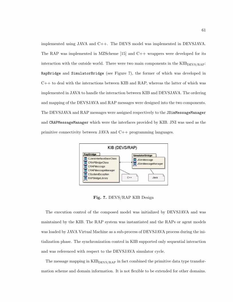
61
implemented using JAVA and C++. The DEVS model was implemented in DEVSJAVA.
The RAP was implemented in MZScheme [15] and C++ wrappers were developed for its
interaction with the outside world. There were two main components in the KIBDEVS/RAP:
RapBridge and SimulatorBridge (see Figure 7), the former of which was developed in
C++ to deal with the interactions between KIB and RAP, whereas the latter of which was
implemented in JAVA to handle the interaction between KIB and DEVSJAVA. The ordering
and mapping of the DEVSJAVA and RAP messages were designed into the two components.
The DEVSJAVA and RAP messages were assigned respectively to the JSimMessageManager
and CRAPMessageManager which were the interfaces provided by KIB. JNI was used as the
primitive connectivity between JAVA and C++ programming languages.
Fig. 7. DEVS/RAP KIB Design
The execution control of the composed model was initialized by DEVSJAVA and was
maintained by the KIB. The RAP system was instantiated and the RAPs or agent models
was loaded by JAVA Virtual Machine as a sub-process of DEVSJAVA process during the ini-
tialization phase. The synchronization control in KIB supported only sequential interaction
and was referenced with respect to the DEVSJAVA simulator cycle.
The message mapping in KIBDEVS/RAP in fact combined the primitive data type transfor-
mation scheme and domain information. It is not flexible to be extended for other domains.
62
The KIBDEVS/RAP supports only sequential interaction control with two participating dis-
parate models. Concurrent execution of the disparate models and the KIB model as well is
not allowed. Furthermore, it is not uncommon that a large-scale complex system consists of
multiple sub-systems with distinct dynamics which are represented by three or more mod-
eling formalisms. How to specify and control the concurrent execution in a heterogeneous
modeling and environment and how to support three or more modeling formalisms to be
composed using KIB approach are not trivial problems and yet to be studied in depth.
The important benefits of this approach include (i) building clear boundaries of separate
problem concerns and (ii) facilitating the formalization of disparate modeling composition.
5.2.2 KIB in DEVS/LP
The KIBDEV S/RAP shows the benefits of composing discrete-event models with RAP agent
model in the domain of vehicle control. In contrast, the process dynamics and the decision
controls presented in the semiconductor manufacturing supply chain systems is far more
complex. A KIBDEV S/LP has been proposed to compose the classes of DEVS and Linear
Optimization formalisms, which was particularly focused on the semiconductor domain with
emphasize on complex information transformations [27, 25].
The multi-formalism model composition via KIB was defined in term of structural and
behaviorial composition specification, the former of which refers to message transforma-
tion whereas the latter specifies the interacting dynamics. The composition was built on
top of the individual modeling characteristics and applied with the semiconductor domain
information. It provides a suite of configurable message transformation and interaction
control scheme that conform to the operations of prototypical semiconductor supply chain
systems. A key aspect of this work is realistic modeling of supply chain systems in term
of both manufacturing processes and decision policies—e.g., a set of detailed discrete-event
63
simulation models as well as a package of messages such as bill-on-hand (BOH), actual-built
(AO) and work-in-progress (WIP), and large-scale linear optimization models, are particu-
larly specified for the semiconductor supply chain systems. KIBDEV S/LP correspondingly
allows specifying the interactions between the discrete processes and decision policies for
the class of semiconductor supply chain systems.
The DEVS/LP composition environment was implemented based on DEVSJAVA and
ILOG OPL Studio [36]. DEVSJAVA provides discrete-event simulation environment,
whereas OPL Studio supports formulation and execution of linear programming models in
an efficient and straightforward way. XML was proposed as KIBDEVS/LP model specifica-
tion language. The execution engine of KIB model was developed using JAVA programming
language, since ILOG OPL Studio provides Java packages to support LP models interacting
with the outside world. The KIB model provides specification of message mappings between
manufacturing process models and LP decision model. Process model sends system state
information via DEVS event messages. KIB transformed the event messages to the cor-
responding input variables in LP model. Similarly, the decision variables output from LP
model is transformed to DEVS input messages in KIB. The message transformation speci-
fication needs to lean on the modeling formalism specifications, the modeling environments
(or languages), and the domain knowledge presented in the messages as well. For example,
in DEVSJAVA, the DEVS message is designed as an Entity object which can carry any
type of data. In OPL Studio, customized data structures can be declared in which case
the LP data interface in OPL Studio is different from a generic mathematical LP data
interface. The mapping between different message types must be well specified. A trans-
formation component was implemented in the KIB execution engine. The transformation
component can read and parse KIB specification (e.g., in term of XML) and then build a set
64
of formalism-independent component models representing the corresponding discrete-event
simulation models specified in the Semiconductor Supply-Demand Network (SSDN) system.
Each of the component models holds a set of system state information which will be relied
on by both the LP decision model and the DEVS process simulation model.
All the data used in the LP decision model has time index, since its computation is
actually based on daily operations of the process model. Although LP model by itself is
not time-based, the data in the model potentially has timing semantics when it is used
to compute strategic plan for the semiconductor manufacturing supply chain. A specific
atomic DEVS model Calendar Time is designed to keep track of the actual logical-time
that has eclipsed in the process models in term of discretized time. The timing property
held in Calendar Time was sent to KIB through DEVS messages for controlling the timing
semantics of the composed model.
Two components DEVSInterface and LPInterface were designed as interfaces for the
DEVS and KIB, and for LP and KIB, respectively. DEVSInterface was designed as a spe-
cific atomic DEVS model. In the DEVSInterface model, two phases {idle, processing} were
specified and their execution sequence within one processing cycle is idle −→ processing −→
idle. This DEVS model can (1) collect state information from other DEVS facility mod-
els through DEVS output events, (2) inform KIB transformation engine to update facility
states, (3) inform LPInterface to activate LP model through java method invocation, and
(4) send out the latest decision plan to Process model. Step (1) and (2) was executed in the
external transition function; Step (3) to (4) was executed in the output function at phase
processing. It shows that the execution of DEVSInterface model is controlled by the DEVS
simulation protocol which is indirectly controlling the concurrency and synchronization of
the composed behavior.
65
In the DEVS/LP composition framework, the execution control of the composite behavior
was specified in term of a DEVS model whose execution was essentially controlled by the
parallel DEVS simulation protocol so as to ensure the timing property, concurrency and
synchronization of the composition. A suit of primitive and composite DEVS models as
well as a set of message types were designed targeting for semiconductor manufacturing
supply chain systems.
There are several limitations of composition framework. Similarly to the DEVS/RAP
composition, this composition framework (or specifically the KIB specification and its ex-
ecution engine) supports only bi-formalism composition. The system execution doesn’t
support parallel execution among the disparate models. Furthermore, it is desirable to
have disparate models configured and executed in a distributed computation environment
to seek for parallel computation and maximal resource utilization. These are all nontrivial
research questions which need further study.
The conceptual basis of the KIB approach is to separate models from their simulation
(or execution engine). A proposed modeling composition framework using KIB is depicted
in Figure 8. With this multi-formalism modeling framework, the characteristics of model
heterogeneity is carried out with KIB specification and its corresponding executor, which
account for the modeling formalism specialties in syntax and behavioral semantics and
provide generalized support for data and control between disparate models. Such layer of
general-purpose multi-formalism model composition can support different domains such as
a distributed system in which the physical process flows and logical decision making can be
executed separately.
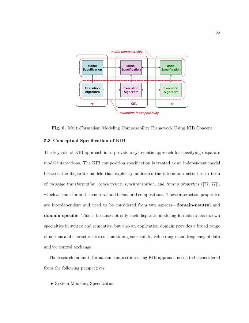
66
Fig. 8. Multi-Formalism Modeling Composability Framework Using KIB Concept
5.3 Conceptual Specification of KIB
The key role of KIB approach is to provide a systematic approach for specifying disparate
model interactions. The KIB composition specification is treated as an independent model
between the disparate models that explicitly addresses the interaction activities in term
of message transformation, concurrency, synchronization, and timing properties ([77, 77]),
which account for both structural and behavioral compositions. These interaction properties
are interdependent and need to be considered from two aspects—domain-neutral and
domain-specific. This is because not only each disparate modeling formalism has its own
specialties in syntax and semantics, but also an application domain provides a broad range
of notions and characteristics such as timing constraints, value ranges and frequency of data
and/or control exchange.
The research on multi-formalism composition using KIB approach needs to be considered
from the following perspectives.
� System Modeling Specification

67
– Number of formalisms involved
Bi-Formalism only two disparate modeling formalisms are involved
Multi-Formalism more than two disparate modeling formalisms are involved
* Some participating formalisms may be considered to be equivalent
– Time synchronization1
The time synchronization is to specify the timing when the interaction occur
among the disparate models, and to ensure that the interaction between the
disparate models doesn’t break the time ordering and message causality for the
holistic composite model
� System Simulation/Execution
We assume that the disparate models are executed in their own simulation/execution
environment.
– Sequential execution: the disparate models and KIB model execute sequen-
tially; no concurrent execution is allowed.
– Parallel execution: it allows for concurrent execution among the disparate
models and KIB model.
5.3.1 Structural Composition Specification
In general, disparate modeling formalisms present distinct specifications on model struc-
ture. The structural composition specification is desired to handle the differences of the
interface structures between disparate models. For example, in the DEVS framework, input
1It is assumed in our research that the process simulation models are periodically con-trolled by the decision model(s)
68
and output ports are used as interface structures for DEVS and non-DEVS model compo-
nents to interact. The interface structure of an (atomic or coupled) DEVS model consists
of sets of input and output ports with message bags to be exchanged with other model
components. The interface structures for a decision model (e.g., LP or MPC model), on
the other hand, may be a set of numerical variables. The structural composition specifica-
tion—message transformation—is to ensure the messages from the simulation models are
properly transformed to their corresponding variable(s) in the decision model(s) and vise
versa. The message transformation must be considered from the aspects of the supporting
(utilized) modeling formalisms, modeling environments, and domain specific knowledge.
5.3.1.1 Model Message Transformation
The message associated with a specific modeling formalism can be categorized as model
messages and control messages, the former of which refer to messages communicating
at the modeling level, whereas the latter refers to the controlling information at simula-
tion/execution level.
The structure of model messages in distinct modeling formalisms are expressed in different
ways. In DEVS modeling, a model message is associated with an atomic model and a port,
and can be specified in the form of <model, port, variable>. The variable can represent
an event which may carry data payload (with diverse data types). In LP or MPC modeling
formalism, no port is used; a model message is generally specified in term of numerical
variables—primitive values, vectors or arrays. The model message can be considered as
<inputVariables, outputVariables>. The composition specification must account for
the distinctions of the interface structures among the disparate modeling formalisms.
The data presented in the modeling formalisms is generally abstract and independent of
message types. The modeling languages, or the modeling environments, in the contrary,
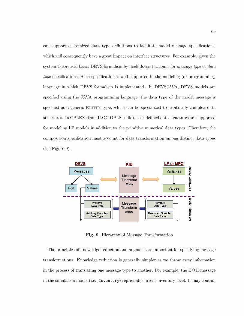
69
can support customized data type definitions to facilitate model message specifications,
which will consequently have a great impact on interface structures. For example, given the
system-theoretical basis, DEVS formalism by itself doesn’t account for message type or data
type specifications. Such specification is well supported in the modeling (or programming)
language in which DEVS formalism is implemented. In DEVSJAVA, DEVS models are
specified using the JAVA programming language; the data type of the model message is
specified as a generic Entity type, which can be specialized to arbitrarily complex data
structures. In CPLEX (from ILOG OPLS tudio), user-defined data structures are supported
for modeling LP models in addition to the primitive numerical data types. Therefore, the
composition specification must account for data transformation among distinct data types
(see Figure 9).
Fig. 9. Hierarchy of Message Transformation
The principles of knowledge reduction and augment are important for specifying message
transformations. Knowledge reduction is generally simpler as we throw away information
in the process of translating one message type to another. For example, the BOH message
in the simulation model (i.e., Inventory) represents current inventory level. It may contain
70
not only the product amount but also the product name. When the message is sent to the
decision model, the name of product may not be necessary. In contrast, knowledge augment
is more difficult. For instance, a numeric output variable of a decision controller represents
a releasing command of a specific product from an explicit inventory (if there exist more
than one inventory) to an explicit customer (if more than one customer is allowed to receive
the product).
In addition to data translation (e.g., from a float to an integer), message transformation
involves data aggregation (from a set of data values to one data value) and disaggregation
(from one data value to a set of data values). The operations of data aggregation include
accumulation, maximum, minimum, etc. The operations of data disaggregation include
average, percentage division, etc.
Therefore, the KIB specification must provide a well-defined mechanism to support the
specification of knowledge reduction/augment and data aggregation/disaggregation.
The control messages are associated with the simulation / execution of the models. The
control messages in DEVS are used for simulation engine execution control—start, pause,
terminate, reset, etc. The control messages in LP or MPC are used for solver execution con-
trol—start, terminate, set number of iterations, etc. The control messages are hidden from
structural composition specification. They are used at level of simulation interoperation.
5.3.1.2 Application Domain Perspective
Model message transformations provide a basis for message transformations from the model-
ing perspective. It is domain-neutral, since it accounts for message syntax and semantics at
the generic modeling formalism level and at the modeling language level. Domain-neutral
message transformation cannot, however, account for composition from a given domain-
specific perspective since rich application domains (e.g., semiconductor supply chain) con-
71
tain rich domain knowledge. The domain knowledge is key in modeling messages and their
transformations at different levels of abstraction, including the low level of process opera-
tions and the high level of decision policies.
In the semiconductor manufacturing supply-chain system, given different planning strate-
gies or control policies, the interaction messages between the process simulation model and
the decision making model can be different on message types, degrees of abstraction and
time scales. For example, the information required by a long-term planning model may
have coarse granularity in comparison to what is required by a short-term tactical controller
model. Therefore, the process simulation model may have to provide different information
based on the requirements of the decision model—i.e., the daily BOH for a tactical con-
troller whereas the weekly BOH for a strategic planner. One of the roles for KIB is to
remove model-specific dependencies between the simulation model and the decision models
by supporting composition at the level of modeling formalisms.
In general, the process simulation model is desired to provide primitive state information
for each processing entity (e.g., WIP in factories, and BOH in inventories) at the end
of each unit (e.g., hourly or daily) processing cycle, whereas the information required by
the decision models can either be primitive or may need to be computed in accordance to
different kinds of planning/control policies. The message transformation needs to account
for abstraction consistency and time unit consistency between the process simulation model
and the decision models. The domain-specific transformations need to be specified on top
of domain-neutral transformations and take the domain knowledge into consideration.
Therefore, the mechanism provided by KIB for specifying structural composition must
be capable of transforming application-neutral knowledge between the chosen modeling
formalisms and be extensible to support domain-specific knowledge transformation as well.
72
5.3.2 Behavioral Composition Specification—Time Synchronization
Time is a crucial property in computer simulations, since the simulation system that is a
computer program represents or emulates the behaviors of another system (called physical
system) over time. There are several different notations of time when discussing simulations
[20]: (1) Physical time, which refers to time in the physical system, (2) Simulation time (or
logical time), which is abstract and defined as a total ordered set of values to model physical
time, and (3) Wallclock time, which refers to time during the execution of the simulation
system. The relationships among the three time notations are discussed in [20]. Briefly,
there is a linear relationship between internals of logical time and internals of physical
time so as to ensure that durations of simulation time correspond properly to durations in
physical time.
In a homogeneous modeling environment, the correct interaction between model com-
ponents is ensured by the individual model behavioral specifications (e.g., time advanced
function and internal/external transition function in an atomic DEVS model) and a well-
defined simulation/execution protocol. In a heterogeneous modeling environment, on the
other hand, although models are representing the same physical system, different modeling
formalisms provide their own approaches for modeling behavioral specification; the simu-
lation/execution protocols are also different. In consequence, the simulation time manage-
ment and synchronization mechanisms of different modeling formalisms can be so distinct
that the dynamic interaction between the disparate models may result in unexpected errors
without a well-defined composite behavioral specification or a well-designed coordination
execution protocol.
In the KIB composition approach, the disparate models are desired to be executed in
their own execution environment. The behavioral specification of the KIB and its execution
73
algorithm is to ensure the disparate models and their interactions are correctly handled,
particularly the timing is processed correctly.
Time synchronization is commonly used to ensure that when a model receives a message
from another model specified in a different modeling formalism, the essential logical time
associated with the message must represent the same physical time as the logical time in
the model does. It must be done at both the modeling specification level and the simula-
tion/execution level. Time synchronization at the modeling level specifies the time instance
at which the interaction should occur between disparate models. It is a key behavioral
property, especially for a system that consists of disparate sub-systems and in which some
sub-system provides controls for other sub-systems at regular time intervals. The specifica-
tion must be configurable to support different interaction frequencies.
For example, in the semiconductor manufacturing supply chain, the discrete process mod-
els simulate manufacturing of physical material flow along a multi-echelon supply network.
One processing cycle along the manufacturing models can represent the behavior over a spe-
cific time segment (i.e., hourly or daily operation), which can be treated as a unit processing
time (TCP )—the time of one operation cycle for a discrete process model. The decision
model, on the other hand, provides operation commands for supply network echelons. The
domain-specific semantics of one execution of the decision model is dependent on the deci-
sion policies it specifies. The decision policy time span per execution for a decision model
is called unit decision time and noted as TCD. The difference on the unit time granularity
determines the different execution frequencies between the process simulation models and
the decision models.
1. When TCD = TCP , the decision model has the same execution frequency as the
process model does.
74
2. When TCD = n ∗ TCP , the execution frequency of the decision model is 1/n of the
processing frequency of the process model. A typical example of this case is that
the process model represents daily operations, whereas the decision model provides
weekly execution plans.
3. When TCD = TCP /n, the decision model is to be executed n times of the frequency
of the process model, since the decision model requires more computation cycles to
resolve the commands needed by the process model. It is considered to be a rare sit-
uation in the real manufacturing supply-chain systems, since the decision policies are
desired to present a higher level of abstraction which treats the dynamic information
collected from the system as the primary data.
Since different decision policies can provide different levels of manufacturing control,
distinct decision models can have different TCDs. The difference on the unit time
granularity between the discrete process model and the decision models determines the
time of interactions between the disparate models. For example, if a process simula-
tion model represents the daily operation, the tactical controller generates weekly com-
mands, and the strategic planner products 4-week planning, the unit time for each model
is TCsimulation = 1, TCcontroller = 7, and TCplanner = 28 respectively. In this case, the
interaction between the process model and the controller model occur every 7 times of the
process model simulating the processing cycle. Similarly, every 28 simulation cycles of the
process model, there is one interaction between the the planner and process simulation
model. If it is assumed that the simulation time of one processing cycle in the process
model is 1, the interaction occurred between the process model and the controller model is
75
at the simulation time of 7, 14, etc. The interaction between the process simulation model
and the planner model is at the simulation time of 28, 56, etc.
As the composition model, the KIB specification with regard to time synchronization
between disparate models must be defined in a flexible way to allow for specifications of
different interaction scenarios.
Time synchronization specification by itself cannot ensure the proper execution of com-
posite behavior due to the different time advance mechanisms among disparate modeling
formalisms. The coordination control at the simulation/execution level is necessary to
achieve time synchronization at runtime. Since the simulation/execution protocol for each
modeling formalism is given, the KIB execution protocol needs to be responsible for ex-
ecution synchronization between disparate models. In fact, the behavioral composition
specification is closely associated with the coordination of simulation/execution protocols
among the process simulation model, the KIB, and the decision model(s).
5.3.3 Control Scheme for Composite Model Execution
The composition specification using the KIB provides a systematic approach for describ-
ing interactions among disparate models at the modeling level. A well-defined composi-
tion/execution control scheme is necessary to ensure the interactions are executed correctly
across a system consisting of the discrete process simulation model, the KIB, and the de-
cision model(s). Each disparate model executes in its own framework and follows its own
execution protocol. As a coordinator, the KIB has its own execution protocol—to coordinate
and synchronize the executions among the disparate models given the KIB specification.
Synchronization control is crucial to ensure the message ordering and causality among the
disparate models. Given different KIB execution algorithms, the disparate models as well
as the KIB model can be executed sequentially or in parallel.
76
5.3.3.1 Sequential Execution Control
In the sequential execution, only one component—one disparate model or the KIB model—is
allowed to be executed at one time. As the coordinator, KIB is responsible for assigning
the execution control to the right model at the proper time instance. For example, when
the process simulation model is assigned to be processed, the simulator executes in its own
simulation framework and sends the latest dynamic states to the KIB when the interaction
with the decision model is needed. Then it stalls its own simulation (i.e., the simulation time
won’t be advanced). The KIB then is allowed to be executed. When the KIB receives the
state messages from the discrete process simulation, it processes the simulation messages
(e.g., transforming and storing the simulation messages). The KIB then generates the input
messages for the appropriate decision model(s) in accordance to its specification and send
them out. The execution control is consequently switched to the receiving model. The
messages may need to be sent to multiple decision models at the same time. The execution
of the decision models must be triggered in the causal order, since there may exist causal
relationships (e.g., data dependency) between any two decision models at certain time
instances. In the case that no causal relationship exists among the receiving models, one
receiving model is selected to be executed. When a decision model receives the messages, it
processes the messages by solving the decision model and sends the computation results back
to the KIB. The KIB will process the computation results by doing message transformation
given the KIB specification. If more than one decision model is in the list of being processed,
the next decision model will be selected to start the execution. When the KIB finishes the
executions of all the decision models, it returns the execution control back to the process
model. When the process model acquires commands, it sends method call to the KIB, KIB
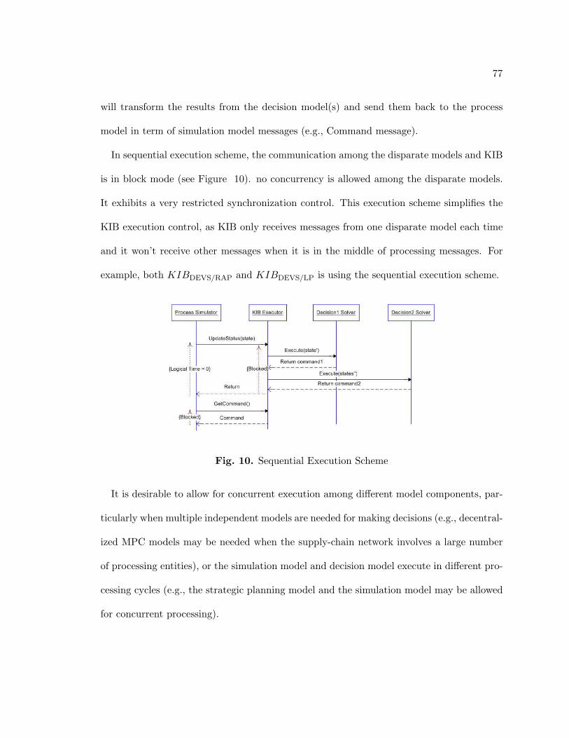
77
will transform the results from the decision model(s) and send them back to the process
model in term of simulation model messages (e.g., Command message).
In sequential execution scheme, the communication among the disparate models and KIB
is in block mode (see Figure 10). no concurrency is allowed among the disparate models.
It exhibits a very restricted synchronization control. This execution scheme simplifies the
KIB execution control, as KIB only receives messages from one disparate model each time
and it won’t receive other messages when it is in the middle of processing messages. For
example, both KIBDEVS/RAP and KIBDEVS/LP is using the sequential execution scheme.
Fig. 10. Sequential Execution Scheme
It is desirable to allow for concurrent execution among different model components, par-
ticularly when multiple independent models are needed for making decisions (e.g., decentral-
ized MPC models may be needed when the supply-chain network involves a large number
of processing entities), or the simulation model and decision model execute in different pro-
cessing cycles (e.g., the strategic planning model and the simulation model may be allowed
for concurrent processing).
78
5.3.3.2 Parallel Execution Control
In parallel execution control, it is allowed to have disparate models execute simultaneously.
For example, the discrete-event process model can continue its simulation when it sends the
latest dynamic status to the KIB and triggers KIB processing interaction messages, since
event-based simulation is desired to support handling unexpected events at any time.(It
is not well supported in the sequential execution scheme.) Concurrent execution of the
disparate decision models is also allowed in the parallel execution scheme. A typical example
of the parallel execution is that a set of decentralized Controllers provide tactical control
policies for a large-scale semiconductor supply-chain system, in which each Controller is
responsible for a particular number of manufacturing processing entities.
In the parallel execution scheme, when the Process model sends the latest states to
the KIB, it can continue its simulation (i.e., the simulation time can be advanced). The
KIB is capable of queueing the messages if it is in the state of processing other messages.
When processing a message from the Process simulation model, KIB can transform the
messages and generate the corresponding input messages to the appropriate decision models
in accordance to the KIB specification. If multiple decision models can be executed in
parallel—e.g., the decentralized Controller can be executed concurrently since they are
independent on each other at the certain time instance, the KIB can send the messages to
all of the Decision models and activates their computations simultaneously. Given the fact
that the Decision models (LP or MPC) are considered to be executed at discrete time, KIB
needs to synchronize the decision model execution by waiting for all the executing decision
models to finish the computation. The synchronization control is necessary in the parallel
execution scheme, as it must ensure the proper time advancement among the disparate
models during their interactions and consequently ensure the timing property of the holistic
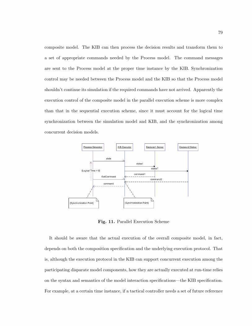
79
composite model. The KIB can then process the decision results and transform them to
a set of appropriate commands needed by the Process model. The command messages
are sent to the Process model at the proper time instance by the KIB. Synchronization
control may be needed between the Process model and the KIB so that the Process model
shouldn’t continue its simulation if the required commands have not arrived. Apparently the
execution control of the composite model in the parallel execution scheme is more complex
than that in the sequential execution scheme, since it must account for the logical time
synchronization between the simulation model and KIB, and the synchronization among
concurrent decision models.
Fig. 11. Parallel Execution Scheme
It should be aware that the actual execution of the overall composite model, in fact,
depends on both the composition specification and the underlying execution protocol. That
is, although the execution protocol in the KIB can support concurrent execution among the
participating disparate model components, how they are actually executed at run-time relies
on the syntax and semantics of the model interaction specifications—the KIB specification.
For example, at a certain time instance, if a tactical controller needs a set of future reference
80
data that needs to be computed by a strategic planner at the same time, the controller and
the planner has to be computed sequentially, since the computation of the controller will be
blocked until the computation of the planner is done. The message dependency is specified
in the message transformation specification which indirectly will impact on the execution of
the holistic composite model. In consequence, deadlock detection may be needed to verify
the composition specification is correct.
5.3.4 Software Design Perspective
Given the characteristics of each modeling specification and execution, a homogeneous soft-
ware environment may not be suitable for multi-formalism composition and execution. For
example, a generic programming language such as C++ or JAVA can be used for imple-
menting discrete-event system dynamic behaviors, whereas it is not convenient for solving
Decision Control model because the solver requires a large-scale computation capability.
In our research, the disparate models are chosen to be implemented in different software
environments.
DEVSJAVA is selected as the DEVS simulation environment for building discrete-event
Process model. DEVSJAVA supports logical concurrent executions among DEVS models
and it provides synchronous simulation control. Object-oriented software methodology is
used given the characteristics of the object-oriented JAVA programming language. It can
provide modifiable and reusable Process model components to support different manufac-
turing supply chain scenarios in a convenient way.
MATLAB [48] is an environment with adequate scientific computation capability, which
is suitable for solving the decision models such as the MPC model. Although MATLAB
provides an MPC toolbox for MPC model design and execution, we have chosen to use
the MPC model designed in [38, 96]. The built-in mathematical functions provided by
81
MATLAB are used for the MPC model design. The MATLABs QP solver is replaced with
the more efficient and robust MATLAB-QP version of the interior point NLP code LOQO
[90]. A JNI package, JMatLink [61], is used for interoperating JAVA and MATLAB.
ILOG OPL Studio [36] is chosen for modeling and solving the planning model like LP,
since the software supports formulation and execution of linear programming models in an
efficient and straightforward way. ILOG OPL Studio provides JAVA packages to support
LP models interacting with the outside world.
5.4 Summary
The Knowledge Interchange Broker approach was introduced to synthesize disparate models
at the modeling level and thus can support formalizing complementary and unique aspects
of complex interacting systems. The conceptual basis of this approach is that the data
and control described in distinct modeling formalisms offer specific syntactic and semantic
contexts which are ideally considered independent of the software design and programming
language choice.
The existing KIB multi-formalism modeling frameworks KIBDEVS/RAP and KIBDEVS/LP
have demonstrated its novel modeling capabilities of synthesizing disparate models. In the
following chapters, the composition of discrete-event simulation and control-theoretic model
(i.e., Model Predictive Control) using KIB approach will be discussed in detail along with
its application in the semiconductor manufacturing supply-chain systems. Particularly, we
will focus on the parallel execution scheme for the execution of the composite model.
CHAPTER 6
BI-FORMALISM COMPOSITION OF DISCRETE-EVENT SIMULATION
AND MODEL PREDICTIVE CONTROL
Given the KIB specification and execution control protocol defined in Chapter 5, we created
KIBDEV S/MPC for composing discrete-event modeling formalism with control-theoretic
Model Predictive Control modeling. A prototype simulation testbed was developed using
the KIBDEV S/MPC . This composition environment supports sequential execution scheme.
6.1 DEVS Modeling for Semiconductor Manufacturing Physical Process
There are three major processes in the semiconductor manufacturing: Fabrication, Test, As-
sembly, and Finish. At the Fabrication process, transistors are built on a silicon water and
then interconnected to form circuits. The working wafers are then tested to sort working
dies into broad functional categories. The dies then go into one or more Assembly processes.
During the Assembly process, dies are cut from the wafers and put into packages. Testing
is also needed for final classification of the packages based on performance ratings. These
semi-finished goods then enter into Finish which includes configuring packages as final prod-
ucts. A set of properties are shown along the manufacturing process: (1) throughput time
distribution (TPT) due to random machine breakdown, (2) stochasticity of manufacturing
yield, (3) distribution of product characteristics, and (4) product asymmetry that allows
faster devices to be configured to run more slowly whereas slow devices cannot be configured
to run faster. Given the principle of demand-driven manufacturing, a set of periodic core
decisions must be made continuously during the manufacturing processes. These decisions
determine how much of what material and when to be released into Fabrication, Assembly,
Test, and Finish factories (or processes).
From a simulation model specification perspective, a model of a semiconductor manufac-
turing supply-chain system can be specified in term of a network consisting of inventory,
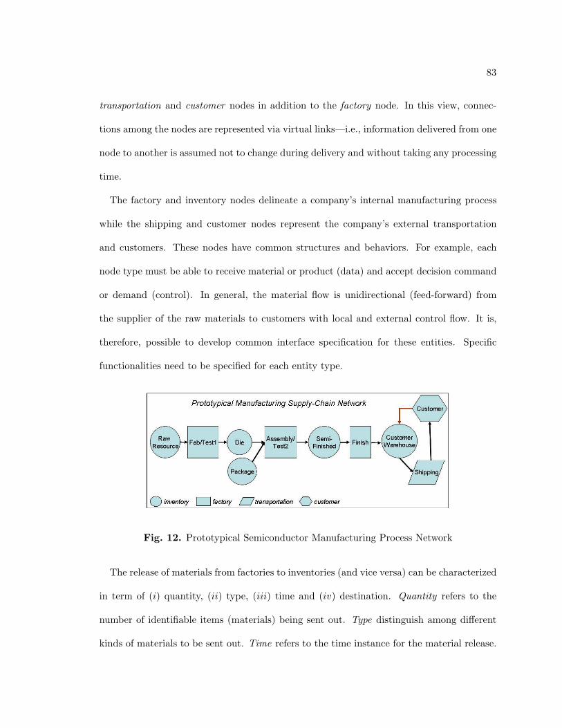
83
transportation and customer nodes in addition to the factory node. In this view, connec-
tions among the nodes are represented via virtual links—i.e., information delivered from one
node to another is assumed not to change during delivery and without taking any processing
time.
The factory and inventory nodes delineate a company’s internal manufacturing process
while the shipping and customer nodes represent the company’s external transportation
and customers. These nodes have common structures and behaviors. For example, each
node type must be able to receive material or product (data) and accept decision command
or demand (control). In general, the material flow is unidirectional (feed-forward) from
the supplier of the raw materials to customers with local and external control flow. It is,
therefore, possible to develop common interface specification for these entities. Specific
functionalities need to be specified for each entity type.
Fig. 12. Prototypical Semiconductor Manufacturing Process Network
The release of materials from factories to inventories (and vice versa) can be characterized
in term of (i) quantity, (ii) type, (iii) time and (iv) destination. Quantity refers to the
number of identifiable items (materials) being sent out. Type distinguish among different
kinds of materials to be sent out. Time refers to the time instance for the material release.
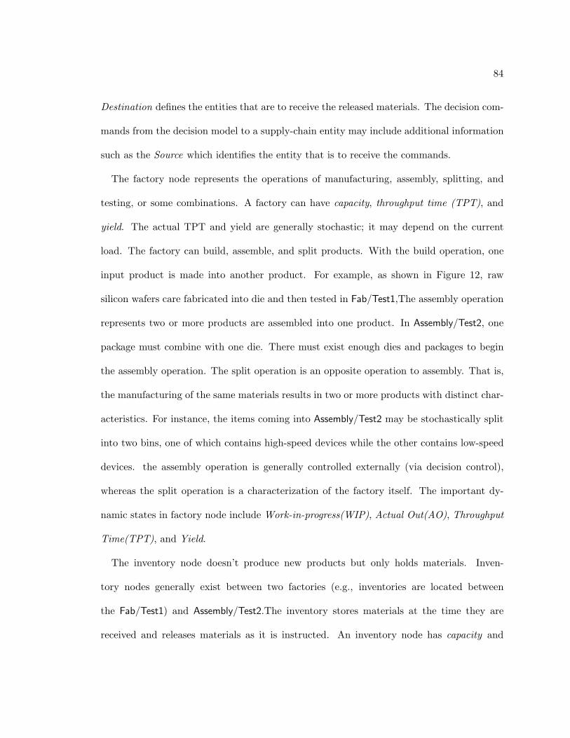
84
Destination defines the entities that are to receive the released materials. The decision com-
mands from the decision model to a supply-chain entity may include additional information
such as the Source which identifies the entity that is to receive the commands.
The factory node represents the operations of manufacturing, assembly, splitting, and
testing, or some combinations. A factory can have capacity, throughput time (TPT), and
yield. The actual TPT and yield are generally stochastic; it may depend on the current
load. The factory can build, assemble, and split products. With the build operation, one
input product is made into another product. For example, as shown in Figure 12, raw
silicon wafers care fabricated into die and then tested in Fab/Test1,The assembly operation
represents two or more products are assembled into one product. In Assembly/Test2, one
package must combine with one die. There must exist enough dies and packages to begin
the assembly operation. The split operation is an opposite operation to assembly. That is,
the manufacturing of the same materials results in two or more products with distinct char-
acteristics. For instance, the items coming into Assembly/Test2 may be stochastically split
into two bins, one of which contains high-speed devices while the other contains low-speed
devices. the assembly operation is generally controlled externally (via decision control),
whereas the split operation is a characterization of the factory itself. The important dy-
namic states in factory node include Work-in-progress(WIP), Actual Out(AO), Throughput
Time(TPT), and Yield.
The inventory node doesn’t produce new products but only holds materials. Inven-
tory nodes generally exist between two factories (e.g., inventories are located between
the Fab/Test1) and Assembly/Test2.The inventory stores materials at the time they are
received and releases materials as it is instructed. An inventory node has capacity and
85
delay. One major dynamic state of an inventory (e.g., Die and Package) is Beginning-on-
hand(BOH)—inventory level (possible with stochasticity) for each product it can hold.
Transportation exists between any two supply-chain entities when one release materials
(or products) to the other. The transportation consumes time, but it may be abstracted
and assumed to occur instantaneously. More precisely, an explicit transportation node is
intended to represent transportation delays—e.g., the Shipping between CustomerWarehouse
and Customer presents transportation delays. The transportation node can be considered
as a special factory node where products cannot be changed and it takes a finite length of
time to be transported from one node to another in the supply network.
The customer node describes customer behaviors. it can send product demands to both
the decision system and manufacturing process system (e.g., customer warehouses) for deci-
sion making and order processing respectively. It can receive products to verify whether the
orders are satisfied or not. Two types of customer demands may be modeled: forecasting
demands and actual demands.
Fiure 12 shows a simplified, prototypical, model of a manufacturing supply-chain net-
work which consists of three factories (i.e., Fab/Test1, Assembly/Test2, and Finish), 5 inven-
tories(i.e., RawResource, Die, Package, Semi-Finished, and CustomerWarehouse), one trans-
portation(Shipping), and one customer (Customer). The directional connections between
any two nodes indicates that the data or control outputs from one node will be delivered
to the other node simultaneously and without any change (e.g., the link between Fab/Test1
and Die in Figure 12).
Ports can be specified as input/output interface for all network nodes. The ports are
distinguishable as data and control input and output ports. A node may have multiple
ports to support sending different products to multiple destinations. The decision of how
86
many (quantity), what (material type), when (time to send), and where (destination) from
a node is determined on the basis of dynamic information of other network nodes as well
as its own. For example, where to send the material from an inventory node is decided by
a decision model, whereas product split is a factory node’s own behavior.
External and local controls are defined for manufacturing process network. The external
control represents the decision commands to the supply-chain network nodes from an inde-
pendent decision model where a formula of certain dynamic information among the process
nodes is specified and solved. For example, the release commands from each inventory can
be determined using the optimization scheme given the current inventory BOH, factory
WIP, customer demands and some constraints among them. Some decisions, however, may
be formulated locally. For instance, an inventory releases a quantity of materials given the
external release command. However, the actual release of the inventory may be constrained
by the maximal capacity of the receiving (downstream) node and its available level (see
Figure 13).
Fig. 13. Local Control Policy for Inventory
Given different objectives for simulating supply-chain systems, the manufacturing process
nodes can be modeled at different levels of abstraction. In particular, the model dynamics
presented here is specified to be used with decision plans—i.e., daily operations along the
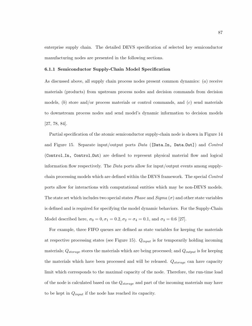
87
enterprise supply chain. The detailed DEVS specification of selected key semiconductor
manufacturing nodes are presented in the following sections.
6.1.1 Semiconductor Supply-Chain Model Specification
As discussed above, all supply chain process nodes present common dynamics: (a) receive
materials (products) from upstream process nodes and decision commands from decision
models, (b) store and/or process materials or control commands, and (c) send materials
to downstream process nodes and send model’s dynamic information to decision models
[27, 78, 84].
Partial specification of the atomic semiconductor supply-chain node is shown in Figure 14
and Figure 15. Separate input/output ports Data ([Data In, Data Out]) and Control
(Control In, Control Out) are defined to represent physical material flow and logical
information flow respectively. The Data ports allow for input/output events among supply-
chain processing models which are defined within the DEVS framework. The special Control
ports allow for interactions with computational entities which may be non-DEVS models.
The state set which includes two special states Phase and Sigma (σ) and other state variables
is defined and is required for specifying the model dynamic behaviors. For the Supply-Chain
Model described here, σ0 = 0, σ1 = 0.2, σ2 = σ4 = 0.1, and σ3 = 0.6 [27].
For example, three FIFO queues are defined as state variables for keeping the materials
at respective processing states (see Figure 15). Qinput is for temporarily holding incoming
materials; Qstorage stores the materials which are being processed; and Qoutput is for keeping
the materials which have been processed and will be released. Qstorage can have capacity
limit which corresponds to the maximal capacity of the node. Therefore, the run-time load
of the node is calculated based on the Qstorage and part of the incoming materials may have
to be kept in Qinput if the node has reached its capacity.
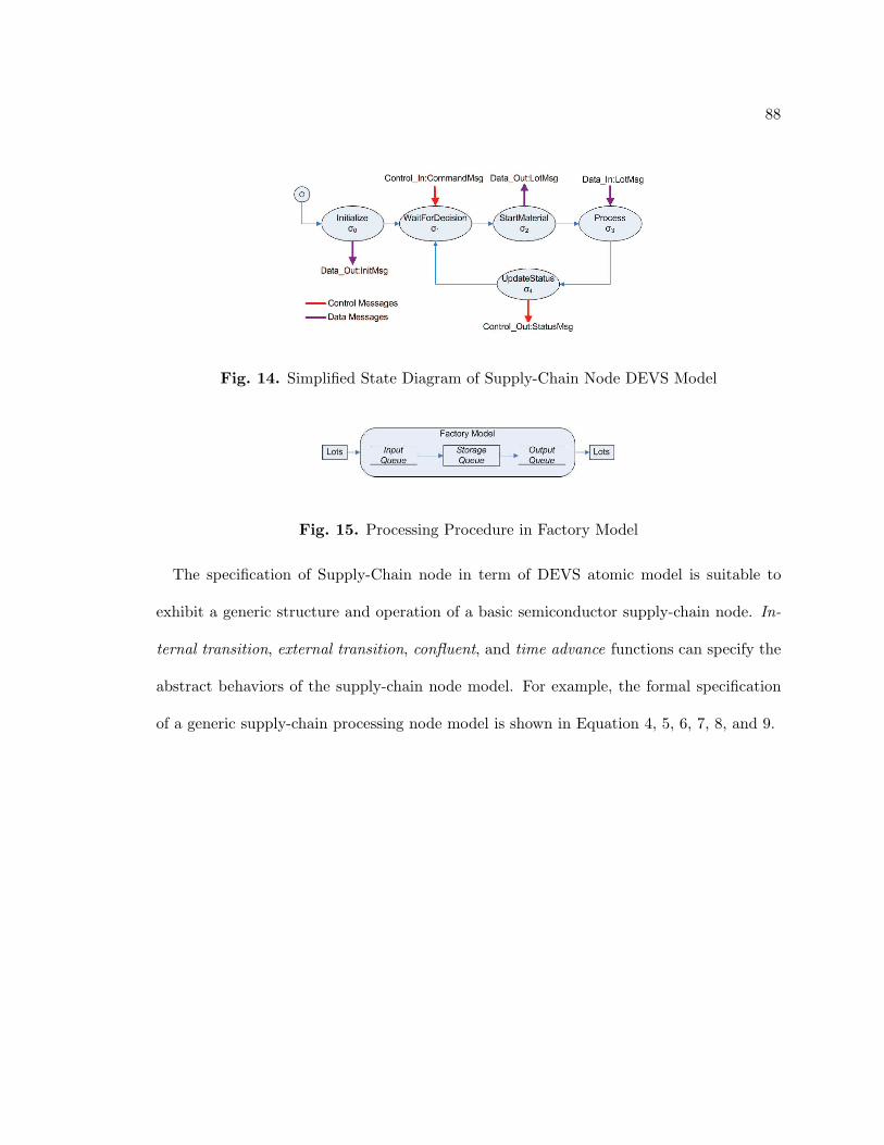
88
Fig. 14. Simplified State Diagram of Supply-Chain Node DEVS Model
Fig. 15. Processing Procedure in Factory Model
The specification of Supply-Chain node in term of DEVS atomic model is suitable to
exhibit a generic structure and operation of a basic semiconductor supply-chain node. In-
ternal transition, external transition, confluent, and time advance functions can specify the
abstract behaviors of the supply-chain node model. For example, the formal specification
of a generic supply-chain processing node model is shown in Equation 4, 5, 6, 7, 8, and 9.
89
M = 〈X,Y, S, δint, δext, δcon, λ, ta〉
// Input ports and values
X = inport× invalues invalues : {Lot, Command}; inport : {Data In,Control In}
// Output ports and values
Y = outport× outvalues outvalues : {Lot, Status}; outport : {Data Out, Control Out}
// State set
S = phase× σ ×Q
phase : {Initialize, WaitForDecision, StartMaterial, Process, UpdateSatus}
σ : <+0,∞
Q : Qinput ×Qoutput ×Qstorage, where the elements for each Qinput, Qoutput and Qstorage
form a FIFO list consisting of the entities from set invalues
(4)
90
// Internal Transition Function
δint(phase, σ,Q) =
s ⇐ (“WaitForDecision”, σ,Q) when phase = “Initialize”
process commands in Qinput when phase = “WaitForDecision”
s ⇐ (“StartMaterial”, σ,Q)
s ⇐ (“Process”, σ,Q) when phase = “StartMaterial”
process lots in Qinput when phase = “Process”
process lots in Qstorage
s ⇐ (“StartMaterial”, σ,Q)
where s ∈ S
(5)
// External Transition Function
δext((phase, σ,Q), e, x) =
add commands in Qinput when phase = “Initialize”∧
s ⇐ (phase, σ′, Q) x ∈{Control In, Command}
add lots in Qinput when phase = “process”∧
s ⇐ (phase, σ′, Q) x ∈ {Data In, Lot}
where s ∈ S
(6)
// Confluent Transition Function
δcon((phase, σ,Q), e, x) = δext(δint(phase, σ,Q), 0, x)(7)
91
// Output Function
λ(phase, σ,Q) =
generate lots from Qoutput when phase = “StartMaterial”
y ⇐ (Data Out, lots)
generate statuses from Qoutput when phase = “UpdateStatus”
y ⇐ (Contro Out, statuses)
where y ∈ Y
(8)
// Time Advanced Function
ta(s) =
σ0 ⇐ σ when phase = “Initialize”
σ1 ⇐ σ when phase = “WaitForDecision”
σ2 ⇐ σ when phase = “StartMaterial”
σ3 ⇐ σ when phase = “Process”
σ4 ⇐ σ when phase = “UpdateStatus”
where s ∈ S and4∑
i=0
σi = T such that 0 ≤ σi < T and T is the duration of
a complete supply chain entity cycle
(9)
Object-oriented concepts and technologies are used to support reuse of the DEVS model
specification. Furthermore, each model type can present its own specialties—e.g., how
to process product lots, and how to calculate processing delays, by extending the basic
specification template. For instance, the detailed message processing within the behavioral
functions are subject to specific model types. The state diagram for the supply-chain
92
node model in Figure 14 depicts the simplified state transitions given external and internal
events. Each phase shown is assigned a finite length of time, at the end of which the model
undergoes either internal or external function.
6.1.1.1 Atomic Factory/Inventory Model
A factory or inventory model extends the basic structure and behavior of a generic supply-
chain model. Factory model specifies manufacturing operations such as building, assem-
bling, testing, splitting products, or some combinations thereof. From the structure per-
spective, an atomic factory model has one pair of data input/out ports and one pair of
control input/output ports. Multiple input/output portsare allowed for different purposes.
For instance, multiple data output ports may be defined to support sending materials to
multiple destinations. From the behavior perspective, the processing procedure follows the
message processing templates defined in the supply-chain model’s behavior functions. Con-
crete message processing functions (e.g., lot processing) need to be specified explicitly to
describe distinct manufacturing operations—i.e., producing new products including assem-
bly or separation operations. Factory/inventory models provide rich generalized data sets
and input/output interfaces to allow for integration with control and decision models [84].
The processing procedure for a (factory/inventory) supply-chain atomic model can be
informally described as follows.
1. At the phase Initialize, certain (factory/inventory) model parameters are set —e.g.,
capacity, normal yield, or TPT distribution.
2. Commands, if there is any from control and decision model(s), arrive as external
messages through Control In port during phase WaitForDecision. Each command
can request some product (lots) to be processed for certain finite period of time.
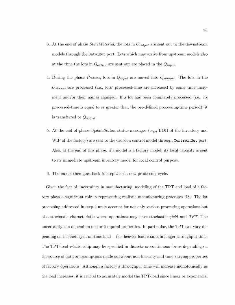
93
3. At the end of phase StartMaterial, the lots in Qoutput are sent out to the downstream
models through the Data Out port. Lots which may arrive from upstream models also
at the time the lots in Qoutput are sent out are placed in the Qinput.
4. During the phase Process, lots in Qinput are moved into Qstorage. The lots in the
Qstorage are processed (i.e., lots’ processed-time are increased by some time incre-
ment and/or their names changed. If a lot has been completely processed (i.e., its
processed-time is equal to or greater than the pre-defined processing-time period), it
is transferred to Qoutput
5. At the end of phase UpdateStatus, status messages (e.g., BOH of the inventory and
WIP of the factory) are sent to the decision control model through Control Out port.
Also, at the end of this phase, if a model is a factory model, its local capacity is sent
to its immediate upstream inventory model for local control purpose.
6. The model then goes back to step 2 for a new processing cycle.
Given the fact of uncertainty in manufacturing, modeling of the TPT and load of a fac-
tory plays a significant role in representing realistic manufacturing processes [78]. The lot
processing addressed in step 4 must account for not only various processing operations but
also stochastic characteristic where operations may have stochastic yield and TPT. The
uncertainty can depend on one or temporal properties. In particular, the TPT can vary de-
pending on the factory’s run-time load —i.e., heavier load results in longer throughput time.
The TPT-load relationship may be specified in discrete or continuous forms depending on
the source of data or assumptions made out about non-linearity and time-varying properties
of factory operations. Although a factory’s throughput time will increase monotonically as
the load increases, it is crucial to accurately model the TPT-load since linear or exponential
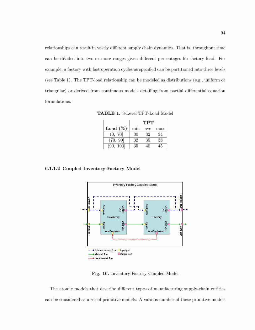
94
relationships can result in vastly different supply chain dynamics. That is, throughput time
can be divided into two or more ranges given different percentages for factory load. For
example, a factory with fast operation cycles as specified can be partitioned into three levels
(see Table 1). The TPT-load relationship can be modeled as distributions (e.g., uniform or
triangular) or derived from continuous models detailing from partial differential equation
formulations.
TABLE 1. 3-Level TPT-Load Model
TPTLoad (%) min ave max
(0, 70] 30 32 34(70, 90] 32 35 38(90, 100] 35 40 45
6.1.1.2 Coupled Inventory-Factory Model
Fig. 16. Inventory-Factory Coupled Model
The atomic models that describe different types of manufacturing supply-chain entities
can be considered as a set of primitive models. A various number of these primitive models
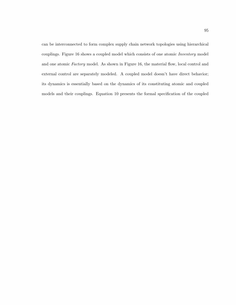
95
can be interconnected to form complex supply chain network topologies using hierarchical
couplings. Figure 16 shows a coupled model which consists of one atomic Inventory model
and one atomic Factory model. As shown in Figure 16, the material flow, local control and
external control are separately modeled. A coupled model doesn’t have direct behavior;
its dynamics is essentially based on the dynamics of its constituting atomic and coupled
models and their couplings. Equation 10 presents the formal specification of the coupled
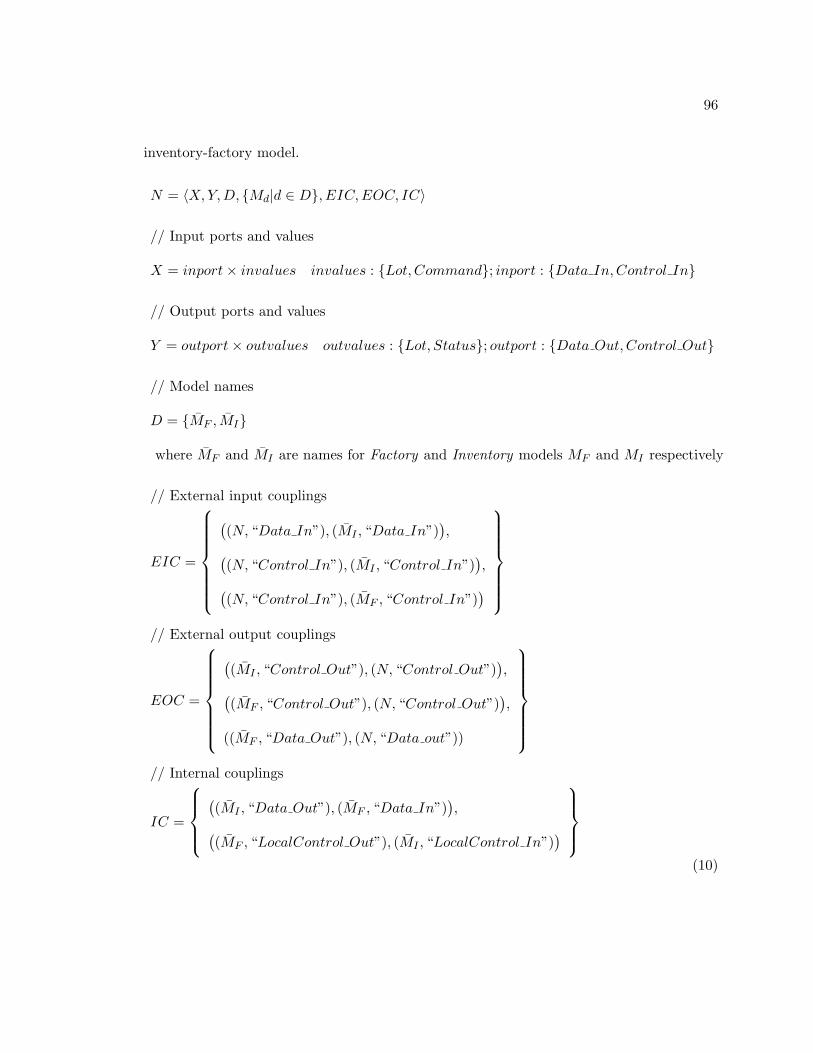
96
inventory-factory model.
N = 〈X,Y, D, {Md|d ∈ D}, EIC, EOC, IC〉
// Input ports and values
X = inport× invalues invalues : {Lot, Command}; inport : {Data In,Control In}
// Output ports and values
Y = outport× outvalues outvalues : {Lot, Status}; outport : {Data Out, Control Out}
// Model names
D = {MF , MI}
where MF and MI are names for Factory and Inventory models MF and MI respectively
// External input couplings
EIC =
((N, “Data In”), (MI , “Data In”)
),
((N, “Control In”), (MI , “Control In”)
),
((N, “Control In”), (MF , “Control In”)
)
// External output couplings
EOC =
((MI , “Control Out”), (N, “Control Out”)
),
((MF , “Control Out”), (N, “Control Out”)
),
((MF , “Data Out”), (N, “Data out”))
// Internal couplings
IC =
((MI , “Data Out”), (MF , “Data In”)
),
((MF , “LocalControl Out”), (MI , “LocalControl In”)
)
(10)
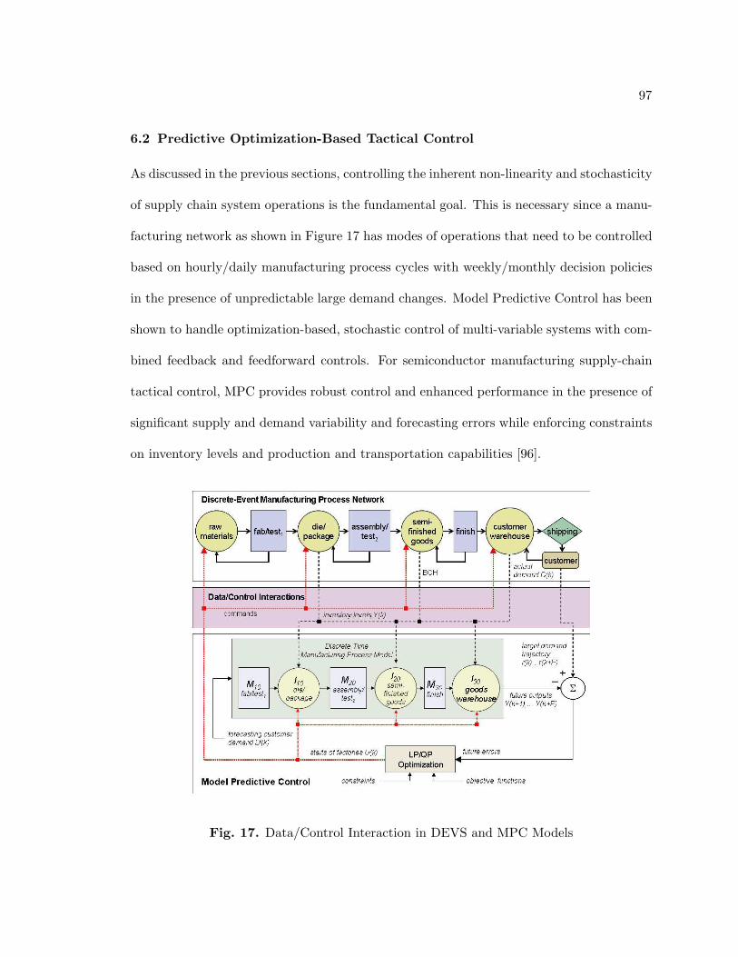
97
6.2 Predictive Optimization-Based Tactical Control
As discussed in the previous sections, controlling the inherent non-linearity and stochasticity
of supply chain system operations is the fundamental goal. This is necessary since a manu-
facturing network as shown in Figure 17 has modes of operations that need to be controlled
based on hourly/daily manufacturing process cycles with weekly/monthly decision policies
in the presence of unpredictable large demand changes. Model Predictive Control has been
shown to handle optimization-based, stochastic control of multi-variable systems with com-
bined feedback and feedforward controls. For semiconductor manufacturing supply-chain
tactical control, MPC provides robust control and enhanced performance in the presence of
significant supply and demand variability and forecasting errors while enforcing constraints
on inventory levels and production and transportation capabilities [96].
Fig. 17. Data/Control Interaction in DEVS and MPC Models
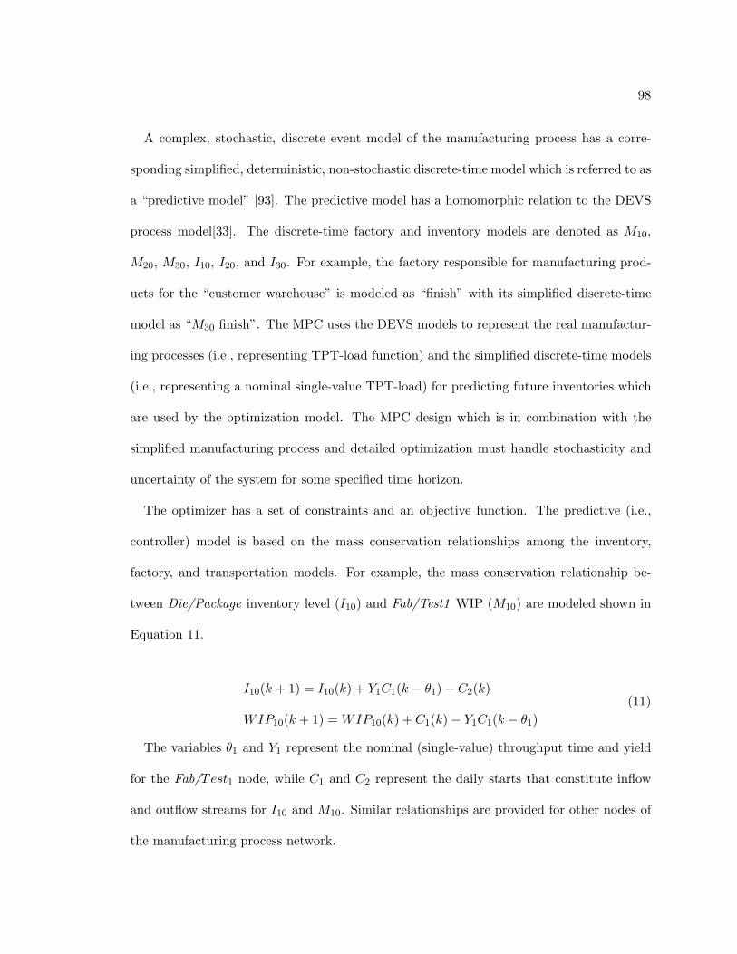
98
A complex, stochastic, discrete event model of the manufacturing process has a corre-
sponding simplified, deterministic, non-stochastic discrete-time model which is referred to as
a “predictive model” [93]. The predictive model has a homomorphic relation to the DEVS
process model[33]. The discrete-time factory and inventory models are denoted as M10,
M20, M30, I10, I20, and I30. For example, the factory responsible for manufacturing prod-
ucts for the “customer warehouse” is modeled as “finish” with its simplified discrete-time
model as “M30 finish”. The MPC uses the DEVS models to represent the real manufactur-
ing processes (i.e., representing TPT-load function) and the simplified discrete-time models
(i.e., representing a nominal single-value TPT-load) for predicting future inventories which
are used by the optimization model. The MPC design which is in combination with the
simplified manufacturing process and detailed optimization must handle stochasticity and
uncertainty of the system for some specified time horizon.
The optimizer has a set of constraints and an objective function. The predictive (i.e.,
controller) model is based on the mass conservation relationships among the inventory,
factory, and transportation models. For example, the mass conservation relationship be-
tween Die/Package inventory level (I10) and Fab/Test1 WIP (M10) are modeled shown in
Equation 11.
I10(k + 1) = I10(k) + Y1C1(k − θ1)− C2(k)
WIP10(k + 1) = WIP10(k) + C1(k)− Y1C1(k − θ1)(11)
The variables θ1 and Y1 represent the nominal (single-value) throughput time and yield
for the Fab/Test1 node, while C1 and C2 represent the daily starts that constitute inflow
and outflow streams for I10 and M10. Similar relationships are provided for other nodes of
the manufacturing process network.
99
In this work, given nodes of a discrete semiconductor manufacturing process, the MPC
manipulates the starts of the factories to satisfy the forecasted customer demands (D′k) given
the actual customer demands (Dk) while maintaining the inventories at the desired levels
(see Figure 17). The controller variables are the inventory levels, the manipulated variables
are starts of the factories and the customer demand is treated as measured disturbance
with anticipation. It is assumed that the manufacturing process is to be controlled on a
daily basis, the MPC manipulates the daily starts of the factories of the semiconductor
manufacturing process model as follows. We have simplified the process model to have one
product:
1. At the initialization, in MPC model, the inventory set-point trajectories are specified.
The model attributes such as average TPT and yield for each factory model are set.
The distribution of some stochastic behaviors, such as distribution of the TPT and
yield, are set in the system simulation model at initialization.
2. At time interval k, the MPC receives the current inventory levels from the system
simulation model. It also receives forecasted customer demands. The system pre-
diction model has the previous inventory levels, the previous starts of each factory,
and the previous customer demands. To calculate the next start for each factory, the
controller operates in two phases:
(a) Estimation. The controller uses all the past measurements, inputs, and the cur-
rent controlled variables to calculate the inventory levels for a prediction horizon.
(b) Optimization. Values of the future inventory level trajectories, anticipated cus-
tomer demands, and constraints are specified over a finite horizon of future sam-
100
pling instants. By solving a constraint optimization problem, it computes the
starts of each factory in the future horizon.
3. The starts at time k are sent to the process simulation model. Each inventory model
then releases products to its downstream factory given its local control policy shown
in Figure 13.
4. At the next time interval k + 1, continue with step 2.
To meet the requirements of the semiconductor supply chain tactical control, the MPC
model is devised to support three degrees of control ([93]). The role of MPC is to provide
robust control given desired (expected) inventory target levels, expected forecast demand
variability, and unanticipated forecast demand. To handle the inherent variability in the
manufacturing processes and customer demand, three kinds of controllers (filters) are used
(see [93] for details). Of particular interest are tuning parameters for these filters. To meet
customer demand, tuning parameters for n inventories αj ∈ [0, 1), j = 1, 2, . . . , n are used to
build safety stocks and thus control unexpected change in demand which in turn will reduce
or otherwise eliminate backlog. The speed at which each inventory can track its target is
directly related to the value of its tuning parameter—smaller α results in faster response
time. To handle measured disturbances (due to expected forecast demand), another tunable
parameter referred to as βj ∈ [0, 1), j = 1, 2, . . . , n is used. Smaller values for these tunable
parameters result in faster response time. To account for unmeasured disturbances, a tuning
parameter fa ∈ [0, 1] needs to be selected. As the value of this parameter decreases, the
impact of the prediction errors due to the stochastic, nonlinear discrete event model is
corresponding reduced. That is, for fa = 0 the controller only relies on the predictive
model alone. In contrast, the controller will compensate all of the prediction errors from
101
stochasticity and uncertainty when fa = 1. These parameters (and other types of filters)
need to be chosen judiciously which can be done using the proposed DEVS/MPC approach
as described in the following sections.
6.3 Hybrid DEVS/MPC using KIB
Earlier, we have shown that discrete-event simulation modeling and MPC tactical control
modeling are fundamentally distinct modeling approaches. They are complementary to each
other for analyzing and solving real-world semiconductor supply-chain problems. However,
a systematic synthesis of the disparate modeling approaches is beyond the “Data/Control
Interactions”. As depicted in Figure 17 it is important to have the Knowledge Interchange
Broker (KIB) framework to formulate the integration of disparate models by explicitly mod-
eling their interactions [79]. The conceptual foundation of KIB is that the data and control
described in each formalism has unique syntactic and semantic specifications and should
not be formulated at the software design and programming language levels, but instead
provides a rigorous and expressive basis for alternative realizations therein. Therefore, in
a neutral setting, KIB distinctly specifies models’ interactions in terms of message trans-
formation, concurrency, synchronization, and timing which must conform to structural and
behavioral compositions of the two formalisms [78]. Furthermore, in order to account for
domain-specific semiconductor supply chain, a suite of data transformations are key to
manage large number of data mappings and relations [27].
For the tactical control of semiconductor manufacturing supply chain, we consider com-
posing a discrete-event process simulation (i.e., DEVS) and a tactical controller (i.e., MPC)
for the simple example shown in Figure 17. The KIB composition specification is consid-
ered as an independent model between the process simulation model and the tactical control
model [78]. Therefore, not only can each participating model be executed within its own
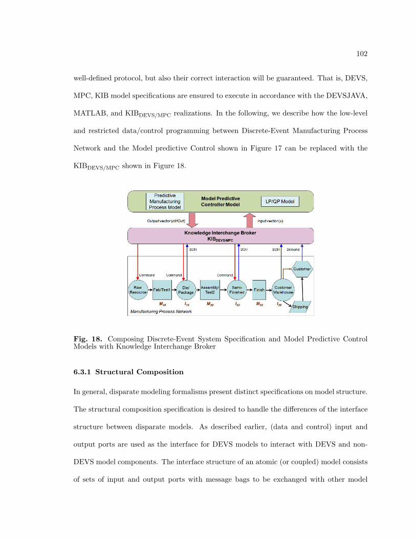
102
well-defined protocol, but also their correct interaction will be guaranteed. That is, DEVS,
MPC, KIB model specifications are ensured to execute in accordance with the DEVSJAVA,
MATLAB, and KIBDEVS/MPC realizations. In the following, we describe how the low-level
and restricted data/control programming between Discrete-Event Manufacturing Process
Network and the Model predictive Control shown in Figure 17 can be replaced with the
KIBDEVS/MPC shown in Figure 18.
Fig. 18. Composing Discrete-Event System Specification and Model Predictive ControlModels with Knowledge Interchange Broker
6.3.1 Structural Composition
In general, disparate modeling formalisms present distinct specifications on model structure.
The structural composition specification is desired to handle the differences of the interface
structure between disparate models. As described earlier, (data and control) input and
output ports are used as the interface for DEVS models to interact with DEVS and non-
DEVS model components. The interface structure of an atomic (or coupled) model consists
of sets of input and output ports with message bags to be exchanged with other model
103
components. The interface structure for a MPC model, on the other hand, is generally nu-
merical variables. The structure composition specification—i.e., message transformation—is
to ensure the messages from the DEVS simulation models are correctly transformed to the
corresponding variables in the MPC model and vice versa.
The structure of DEVS messages is associated with an atomic model and its ports; a
message can represent an event which may carry data payload (with diverse data types).
Given the DEVS abstract theoretical basis, by itself it does not account for message type
or data type specifications. Such specifications are subject to the concrete modeling speci-
fications such as Object-Oriented DEVS and its realization. An example of the structural
specification of an inventory model in DEVSJAVA is given in Equation 12.
X = {(Data In, Lot), (Control In, Command), (LocalControl In, Capacity)}
Y = {(Data Out, Lot), (Contro Out, [BOH,AO])}(12)
The set of inputs and outputs are X and Y with (port, data) structure representing port
name and data type. The data type can be arbitrarily complex such as Lot which contains
a collection of multiple product types with different cardinalities. In our research, Lot is
modeled to have default or customized size (e.g., 100 products per lot).
For the MPC model, its discrete-time predictive model (see in Figure 17) and optimizer do
not use ports. Instead, the interface structural specification of MPC is generally specified in
term of vector variables. The input to the controller from the simulation system is a vector
of controlled variables and a vector of measured disturbance variables, while the output from
the controller to the simulation system is a vector of manipulated variables (see Figure 17).
As in DEVSJAVA, realizations of the MPC and its predictive model in concrete simulation
environments such as SIMULINK may have ports and values. In addition to the primitive
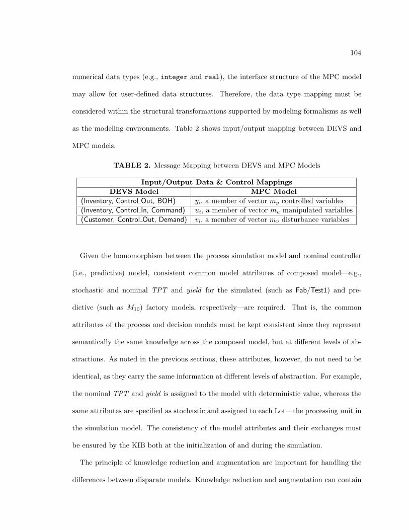
104
numerical data types (e.g., integer and real), the interface structure of the MPC model
may allow for user-defined data structures. Therefore, the data type mapping must be
considered within the structural transformations supported by modeling formalisms as well
as the modeling environments. Table 2 shows input/output mapping between DEVS and
MPC models.
TABLE 2. Message Mapping between DEVS and MPC Models
Input/Output Data & Control MappingsDEVS Model MPC Model
(Inventory, Control Out, BOH) yi, a member of vector my controlled variables(Inventory, Control In, Command) ui, a member of vector mu manipulated variables(Customer, Control Out, Demand) vi, a member of vector mv disturbance variables
Given the homomorphism between the process simulation model and nominal controller
(i.e., predictive) model, consistent common model attributes of composed model—e.g.,
stochastic and nominal TPT and yield for the simulated (such as Fab/Test1) and pre-
dictive (such as M10) factory models, respectively—are required. That is, the common
attributes of the process and decision models must be kept consistent since they represent
semantically the same knowledge across the composed model, but at different levels of ab-
stractions. As noted in the previous sections, these attributes, however, do not need to be
identical, as they carry the same information at different levels of abstraction. For example,
the nominal TPT and yield is assigned to the model with deterministic value, whereas the
same attributes are specified as stochastic and assigned to each Lot—the processing unit in
the simulation model. The consistency of the model attributes and their exchanges must
be ensured by the KIB both at the initialization of and during the simulation.
The principle of knowledge reduction and augmentation are important for handling the
differences between disparate models. Knowledge reduction and augmentation can contain
105
data aggregation and disaggregation. The former is to combine multiple data values (or
a set of messages) into a single data value (a message) and the later defines the inverse.
For example, a MPC data variable may need to be disaggregated so that it can be sent
to multiple DEVS input ports. Knowledge reduction is generally simpler since it throws
away information in the process of translating one message type to another. For example,
the message BOH in the DEVS inventory model represents current inventory level. It may
contain not only the product amount but also the product name. When the message is
transformed to an MPC variable, the name may be superfluous. In contrast, knowledge
augmentation is more challenging. For instance, the manipulated variable sent from the
MPC to the DEVS model represent the release command for certain product from a specific
inventory. The MPC output variables are augmented with port names as DEVS message
based on the MPC and DEVS model specifications, Control Out and Control In ports,
and message discovery which allows each atomic DEVS model to identify whether or not a
message is sent to it or not [84].
Given the discussion above, the KIBDEVS/MPC can be defined as a set of inputs, outputs,
and functions([77]): KIBDEVS/MPC = 〈I, O, F 〉. The input and output sets are defined
as I = IDEV S⋃
IMPC and O = ODEV S⋃
OMPC . IDEV S and IMPC sets represent the
inputs from DEVS and MPC models. Similarly, ODEV S and OMPC sets represent outputs
to DEVS and MPC models. F = G⋃
H represent sets of mapping and transformation
mappings. G = IDEV S 7→ OMPC and H = IMPC 7→ ODEV S where G = {g1, · · · , gm}
and H = {h1, · · · , hn}. Functions gi, i ∈ 1, · · · ,m and hj , j ∈ 1, · · · , n can be defined as
y = f(x, s, t) where x and y are input and output variables with s and t representing state
and time. State can be defined in terms of I and O sets. The functions gi and hj are
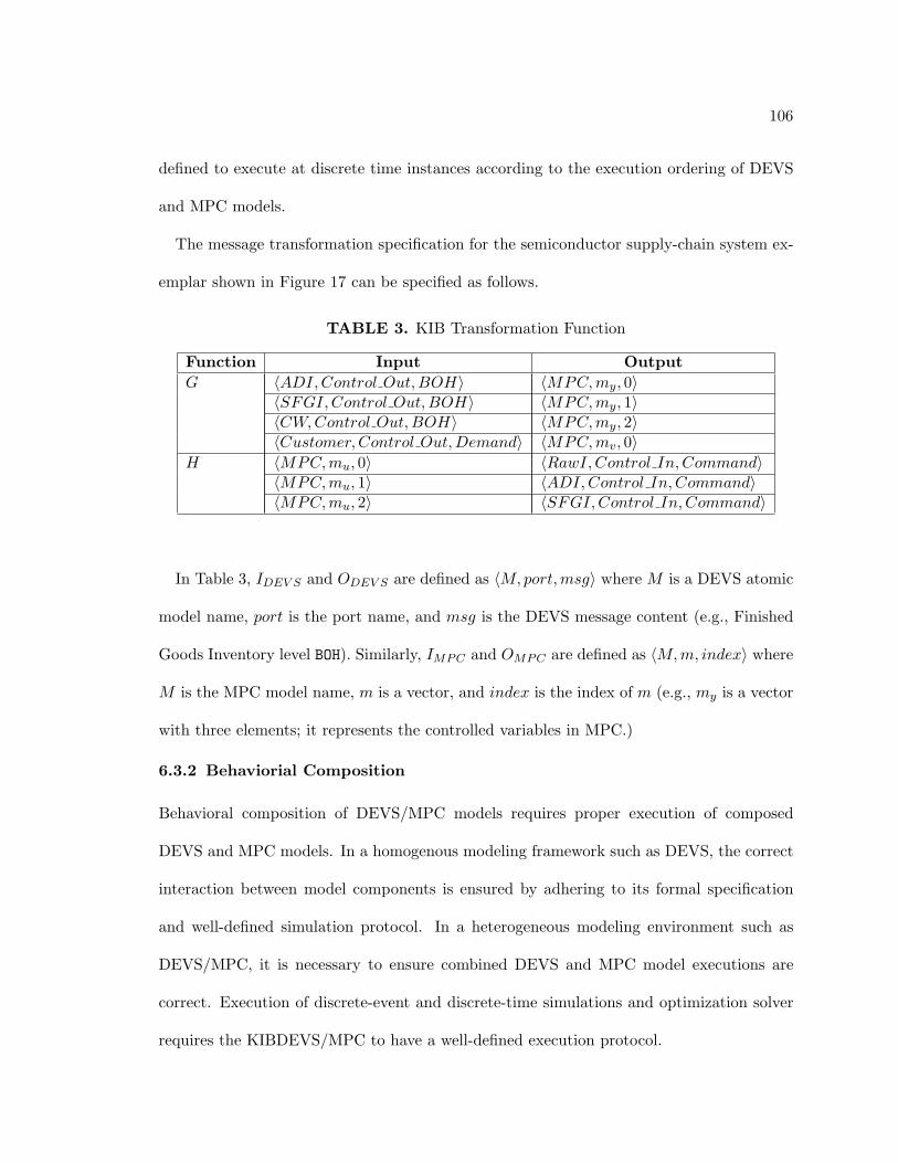
106
defined to execute at discrete time instances according to the execution ordering of DEVS
and MPC models.
The message transformation specification for the semiconductor supply-chain system ex-
emplar shown in Figure 17 can be specified as follows.
TABLE 3. KIB Transformation Function
Function Input OutputG 〈ADI,Control Out, BOH〉 〈MPC, my, 0〉
〈SFGI, Control Out,BOH〉 〈MPC, my, 1〉〈CW,Control Out, BOH〉 〈MPC, my, 2〉〈Customer,Control Out, Demand〉 〈MPC, mv, 0〉
H 〈MPC, mu, 0〉 〈RawI,Control In, Command〉〈MPC, mu, 1〉 〈ADI,Control In, Command〉〈MPC, mu, 2〉 〈SFGI,Control In,Command〉
In Table 3, IDEV S and ODEV S are defined as 〈M, port,msg〉 where M is a DEVS atomic
model name, port is the port name, and msg is the DEVS message content (e.g., Finished
Goods Inventory level BOH). Similarly, IMPC and OMPC are defined as 〈M, m, index〉 where
M is the MPC model name, m is a vector, and index is the index of m (e.g., my is a vector
with three elements; it represents the controlled variables in MPC.)
6.3.2 Behaviorial Composition
Behavioral composition of DEVS/MPC models requires proper execution of composed
DEVS and MPC models. In a homogenous modeling framework such as DEVS, the correct
interaction between model components is ensured by adhering to its formal specification
and well-defined simulation protocol. In a heterogeneous modeling environment such as
DEVS/MPC, it is necessary to ensure combined DEVS and MPC model executions are
correct. Execution of discrete-event and discrete-time simulations and optimization solver
requires the KIBDEVS/MPC to have a well-defined execution protocol.
107
Both DEVS and the MPC’s predictive models have well-defined logical timing properties.
The former has a continuous time-base while the latter has a discrete time-base. Since
the predictive model executes using periodic time-stepping, the KIB’s input and output
events can be synchronized using a discrete time logical clock. This is appropriate as the
timing in discrete-event manufacturing network model is a multiple of the timing of the
predictive model. The discrete-time predictive model can run at the same, faster, or slower
frequency as the manufacturing processing. For example, the manufacturing network model
can simulate daily operations, while the predictive model can have monthly time horizon
and computing daily factory starts. Therefore, causal ordering of all events produced and
consumed across DEVS, KIBDEVS/MPC, and MPC models must be guaranteed.
The DEVS state variables must be updated such that output/input causality and cor-
rect logical timing is satisfied. This requires proper specification for the KIBDEVS/MPC in
order to guarantee correct execution of all DEVS models. Similarly, from the MPC point
of view, KIBDEVS/MPC must ensure correct execution of the MPC model. The task of
the KIBDEVS/MPC, therefore, is to send and receive controlled variables (status) and ma-
nipulated variables (command) to/from the MPC model (i.e., predictive and optimization
models). While the states of the predictive model remain static for a fixed period of logical
time, the optimization solver consumes wall clock time. More specifically, given that the
simulation time of the predictive model is known and the wall clock time consumed for the
optimization solver can vary depending on the optimization problem and computational
resources, it is necessary to define the MPC to consume no logical time in relationship
to the DEVS simulation and KIBDEVS/MPC models. Since the role of the MPC is to re-
ceive states and send commands from/to the DEVS simulation models at the start and
end of every simulation and decision interaction cycle, we model the KIBDEVS/MPC exe-
108
cution cycle to consume logical time. The execution logical time can be a multiple of the
DEVS (Supply Chain node) simulation logical time cycle. Given the timing properties of
DEVS, KIBDEVS/MPC, and MPC as well as a sequential execution scheme among them, we
define the KIBDEVS/MPC models to execute according to the DEVS logical time and the
MPC to consume no logical time. With this specification, the KIBDEVS/MPC specification
allows for synchronizing the DEVS simulation cycle and MPC execution cycle; therefore,
the KIBDEVS/MPC execution cycle and DEVS simulation cycle may have one-to-many and
many-to-many relationships.
Figure 19 shows the DEVS and the KIBDEVS/MPC simulation and execution cycles with
data and control messages. For simplicity, states and events of the inventory model are not
shown (for details refer to the previous section). Also only a partial set of events important
in illustrating the interactions among DEVS, KIBDEVS/MPC, and MPC are depicted. These
events are specified in terms of an Inventory model receiving command (e1) from MPC via
KIBDEVS/MPC, Inventory model sending materials (e2) via the Inventory-Factory internal
coupling and the Factory model receiving the materials (e3), Inventory model sending state
updates to KIBDEVS/MPC and thus to MPC (e4), and Factory model sending its local
capacity (e5) which are received by the Inventory model in the next simulation cycle. It is
important to note that the times at which events e1 and e4 occur are not fixed—i.e., the
DEVS models (e.g., Inventory) are event driven as opposed to discrete time stepping.
The ability of the Inventory model to handle events in some designated states —i.e.,
WaitForDecision in simulation cycle m1—is key in handling lack of a priori knowledge,
since the time at which e1 occurs cannot be predicted. e1 may be received at any time
during the WaitForDecision phase but it must be received before the model’s internal
transition events. In another case, for example in Factory model, events e2 and e3 may
109
occur simultaneously and are handled based on how the confluent function is specified—i.e.,
e2 is handled immediately before e3. As shown, due to internal interactions among the
manufacturing nodes, the atomic and coupled models undergo state changes at a higher
rate of frequency as compared with the KIBDEVS/MPC execution cycle. In particular, the
DEVS simulation goes through several cycles while the KIBDEVS/MPC goes through one
execution cycle. For the example shown in Figure 19, the simulation cycle m consists of
sub-cycles (i.e., m1, m2, m3, and m4) when viewed from the KIBDEVS/MPC execution cycle
j. As mentioned above, the DEVS and KIBDEVS/MPC can interact such that each DEVS
simulation cycle is a multiple of a KIBDEVS/MPC execution cycle.
For the Supply Chain models, the time period beginning from sending out state infor-
mation to receiving control message is dependent on the frequency specified between the
discrete-event manufacturing process and predictive control models. If the discrete-event
and discrete-time models have the same logical time frequency, the manufacturing network
node model must receive control messages before it starts a new manufacturing process cycle
(see Figure 19). If these disparate models run in different frequencies, the KIBDEVS/MPC
will handle sending and receiving appropriate DEVS and MPC status and control messages
at appropriate manufacturing process cycle. For example, if the manufacturing process
model runs twice the frequency of the MPC model, once the Inventory model receives a
control message in phase WaitForDecision, it will use the control command next time it
enters this phase and only in the next iteration it will use an updated control command.
Similarly, the Inventory model sends its inventory level every other time it enters the phase
UpdateStatus. The frequency of state updates and control commands are ensured to happen
together—i.e., the KIBDEVS/MPC specification ensures that the DEVS and MPC cycles are
synchronized in order to have the control commands to be consistent with the inventory val-
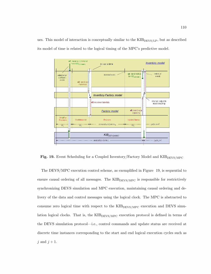
110
ues. This model of interaction is conceptually similar to the KIBDEVS/LP, but as described
its model of time is related to the logical timing of the MPC’s predictive model.
Fig. 19. Event Scheduling for a Coupled Inventory/Factory Model and KIBDEVS/MPC
The DEVS/MPC execution control scheme, as exemplified in Figure 19, is sequential to
ensure causal ordering of all messages. The KIBDEVS/MPC is responsible for restrictively
synchronizing DEVS simulation and MPC execution, maintaining causal ordering and de-
livery of the data and control messages using the logical clock. The MPC is abstracted to
consume zero logical time with respect to the KIBDEVS/MPC execution and DEVS simu-
lation logical clocks. That is, the KIBDEVS/MPC execution protocol is defined in terms of
the DEVS simulation protocol—i.e., control commands and update status are received at
discrete time instances corresponding to the start and end logical execution cycles such as
j and j + 1.
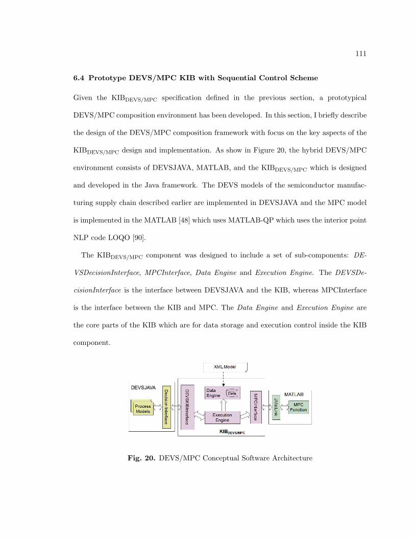
111
6.4 Prototype DEVS/MPC KIB with Sequential Control Scheme
Given the KIBDEVS/MPC specification defined in the previous section, a prototypical
DEVS/MPC composition environment has been developed. In this section, I briefly describe
the design of the DEVS/MPC composition framework with focus on the key aspects of the
KIBDEVS/MPC design and implementation. As show in Figure 20, the hybrid DEVS/MPC
environment consists of DEVSJAVA, MATLAB, and the KIBDEVS/MPC which is designed
and developed in the Java framework. The DEVS models of the semiconductor manufac-
turing supply chain described earlier are implemented in DEVSJAVA and the MPC model
is implemented in the MATLAB [48] which uses MATLAB-QP which uses the interior point
NLP code LOQO [90].
The KIBDEVS/MPC component was designed to include a set of sub-components: DE-
VSDecisionInterface, MPCInterface, Data Engine and Execution Engine. The DEVSDe-
cisionInterface is the interface between DEVSJAVA and the KIB, whereas MPCInterface
is the interface between the KIB and MPC. The Data Engine and Execution Engine are
the core parts of the KIB which are for data storage and execution control inside the KIB
component.
Fig. 20. DEVS/MPC Conceptual Software Architecture
112
The responsibility of the DEVSKIBInterface is to pass data messages from the DEVS
models to the KIBDEVS/MPC and vise versa. The message includes InitMsg and StatusMsg
from DEVS to KIB and CommandMsg from KIB to DEVS. A special atomic model De-
cisionInterface is specified as a proxy between the DEVS models and the KIBDEVS/MPC.
It collects the state messages from the process simulation models through input ports and
then transfers them to the KIBDEVS/MPC. Similarly, it retrieves control messages from the
KIBDEVS/MPC via DEVSKIBInterface and sends them to the process models through output
ports at appropriate time instances. The interaction of DecisionInterface and the process
simulation models is through DEVS ports, whereas the interaction of DecisionInterface and
the KIBDEVS/MPC uses method invocations. In addition, DecisionInterface receives periodic
TimeMsg from an atomic model Clock which is used to execute at discrete time intervals
between the DEVS and MPC models. Therefore, the DecisitionInterface not only is acting
as as a bridge between the process simulation model and KIB, but also is responsible for
synchronization between DEVS and MPC—utilizing DEVS simulation protocol.
The MPCInterface interface defines interactions between the KIB and the MPC. The
MPC is defined as an MPC function — Y Out = mpcFunction(time, U), where time ∈
N , U ∈ <4, and Y Out ∈ <3. Here time is an input variable representing a discretized
time index. The controlled input variable U is a vector. The manipulated variable Y Out
is the output variable. Both U and Y Out variables are of the same type (i.e., double).
The functionality of the MPCInterface includes (a) loading the MPC function file to the
appropriate internal MATLAB workspace, (b) transforming the MPC model in the KIB
to the corresponding MATLAB function call, (c) making the MATLAB call through the
JMatLink [61] which is based on the Java JNI, and (d) transforming the output variables
from MATLAB to the KIB.
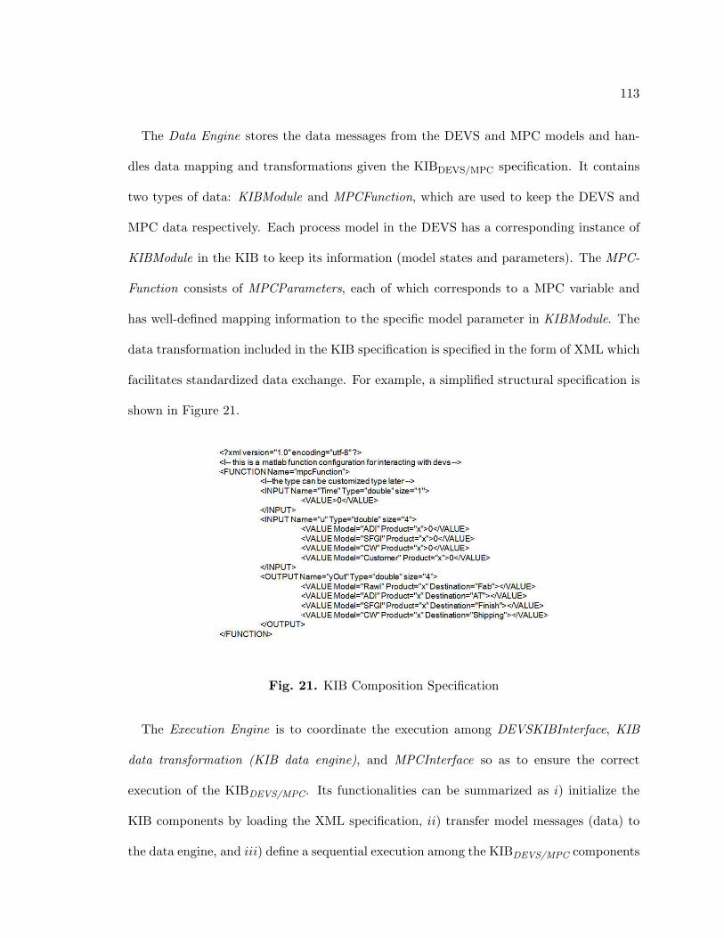
113
The Data Engine stores the data messages from the DEVS and MPC models and han-
dles data mapping and transformations given the KIBDEVS/MPC specification. It contains
two types of data: KIBModule and MPCFunction, which are used to keep the DEVS and
MPC data respectively. Each process model in the DEVS has a corresponding instance of
KIBModule in the KIB to keep its information (model states and parameters). The MPC-
Function consists of MPCParameters, each of which corresponds to a MPC variable and
has well-defined mapping information to the specific model parameter in KIBModule. The
data transformation included in the KIB specification is specified in the form of XML which
facilitates standardized data exchange. For example, a simplified structural specification is
shown in Figure 21.
Fig. 21. KIB Composition Specification
The Execution Engine is to coordinate the execution among DEVSKIBInterface, KIB
data transformation (KIB data engine), and MPCInterface so as to ensure the correct
execution of the KIBDEVS/MPC. Its functionalities can be summarized as i) initialize the
KIB components by loading the XML specification, ii) transfer model messages (data) to
the data engine, and iii) define a sequential execution among the KIBDEVS/MPC components
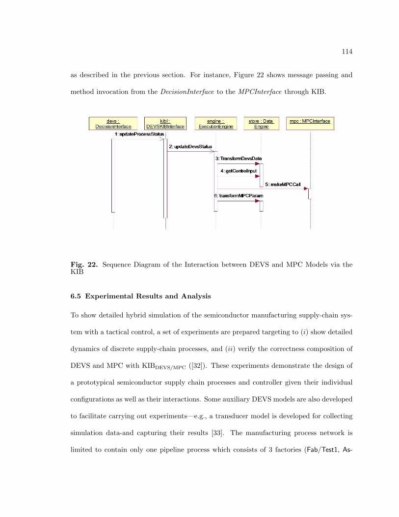
114
as described in the previous section. For instance, Figure 22 shows message passing and
method invocation from the DecisionInterface to the MPCInterface through KIB.
Fig. 22. Sequence Diagram of the Interaction between DEVS and MPC Models via theKIB
6.5 Experimental Results and Analysis
To show detailed hybrid simulation of the semiconductor manufacturing supply-chain sys-
tem with a tactical control, a set of experiments are prepared targeting to (i) show detailed
dynamics of discrete supply-chain processes, and (ii) verify the correctness composition of
DEVS and MPC with KIBDEVS/MPC ([32]). These experiments demonstrate the design of
a prototypical semiconductor supply chain processes and controller given their individual
configurations as well as their interactions. Some auxiliary DEVS models are also developed
to facilitate carrying out experiments—e.g., a transducer model is developed for collecting
simulation data-and capturing their results [33]. The manufacturing process network is
limited to contain only one pipeline process which consists of 3 factories (Fab/Test1, As-
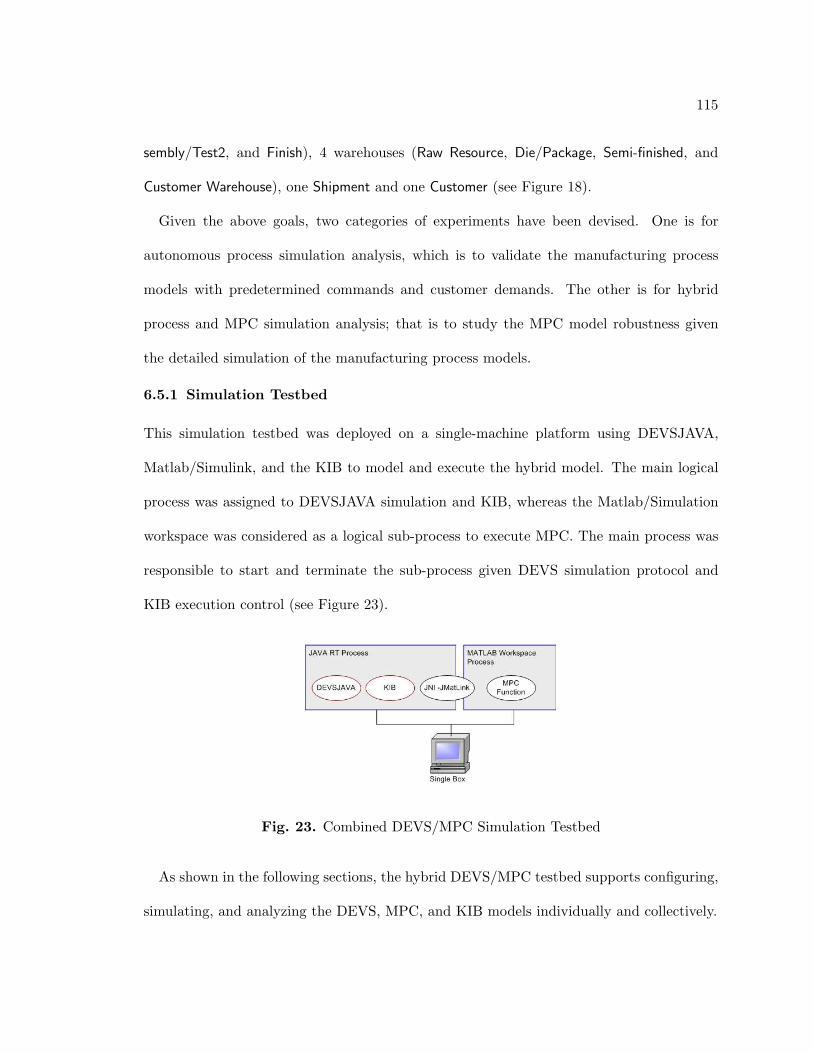
115
sembly/Test2, and Finish), 4 warehouses (Raw Resource, Die/Package, Semi-finished, and
Customer Warehouse), one Shipment and one Customer (see Figure 18).
Given the above goals, two categories of experiments have been devised. One is for
autonomous process simulation analysis, which is to validate the manufacturing process
models with predetermined commands and customer demands. The other is for hybrid
process and MPC simulation analysis; that is to study the MPC model robustness given
the detailed simulation of the manufacturing process models.
6.5.1 Simulation Testbed
This simulation testbed was deployed on a single-machine platform using DEVSJAVA,
Matlab/Simulink, and the KIB to model and execute the hybrid model. The main logical
process was assigned to DEVSJAVA simulation and KIB, whereas the Matlab/Simulation
workspace was considered as a logical sub-process to execute MPC. The main process was
responsible to start and terminate the sub-process given DEVS simulation protocol and
KIB execution control (see Figure 23).
Fig. 23. Combined DEVS/MPC Simulation Testbed
As shown in the following sections, the hybrid DEVS/MPC testbed supports configuring,
simulating, and analyzing the DEVS, MPC, and KIB models individually and collectively.
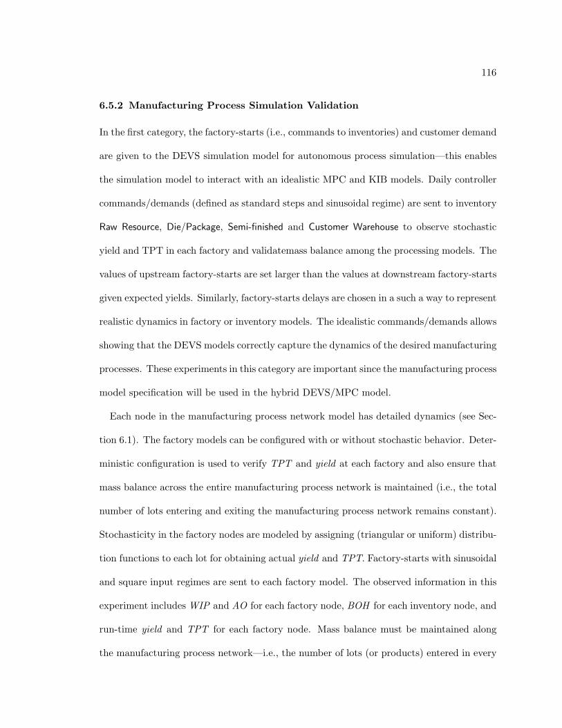
116
6.5.2 Manufacturing Process Simulation Validation
In the first category, the factory-starts (i.e., commands to inventories) and customer demand
are given to the DEVS simulation model for autonomous process simulation—this enables
the simulation model to interact with an idealistic MPC and KIB models. Daily controller
commands/demands (defined as standard steps and sinusoidal regime) are sent to inventory
Raw Resource, Die/Package, Semi-finished and Customer Warehouse to observe stochastic
yield and TPT in each factory and validatemass balance among the processing models. The
values of upstream factory-starts are set larger than the values at downstream factory-starts
given expected yields. Similarly, factory-starts delays are chosen in a such a way to represent
realistic dynamics in factory or inventory models. The idealistic commands/demands allows
showing that the DEVS models correctly capture the dynamics of the desired manufacturing
processes. These experiments in this category are important since the manufacturing process
model specification will be used in the hybrid DEVS/MPC model.
Each node in the manufacturing process network model has detailed dynamics (see Sec-
tion 6.1). The factory models can be configured with or without stochastic behavior. Deter-
ministic configuration is used to verify TPT and yield at each factory and also ensure that
mass balance across the entire manufacturing process network is maintained (i.e., the total
number of lots entering and exiting the manufacturing process network remains constant).
Stochasticity in the factory nodes are modeled by assigning (triangular or uniform) distribu-
tion functions to each lot for obtaining actual yield and TPT. Factory-starts with sinusoidal
and square input regimes are sent to each factory model. The observed information in this
experiment includes WIP and AO for each factory node, BOH for each inventory node, and
run-time yield and TPT for each factory node. Mass balance must be maintained along
the manufacturing process network—i.e., the number of lots (or products) entered in every
117
node and across the entire manufacturing process ensure no products are lost or generated
extraneously.
Fig. 24. Fab/Test1 Starts and Actual Outs with Different Lot Sizes
Figure 24 shows that, Lot size, which is defined as minimal processing unit, plays an
important role in processing dynamics, since it affects directly system’s stochastic behavior.
For example, when the Lot Size is set as maximum in which case stochastic TPT values
generated from triangular distributions are assigned to one lot which includes the amount
of all materials flowing into a factory, the simulation results showed that there existed
great variance on AO from a factory model (e.g., from 0 on one day to several thousands
on the next day), which directly caused dramatic change on factory load. This obviously
didn’t represent the realistic behavior of a factory in semiconductor supply chain process.
Therefore, an appropriate choice of lot size can have great impact on the dynamics of the
system. Given some experiments with different lot size (e.g., maximum, 100, 50, 20 and
10), it has been shown that the smaller size gives smoother behavior in a factory model.
However, in consequence, smaller lot size requires more simulation time, which can affect
the performance of the process and therefore the combined DEVS/MPC simulation (see
118
Section 6.5.4). The tradeoff between lot size and system performance should be taken into
consideration. The simulation results with (lotsize = 50) in our experiments have presented
practical dynamics of the system with good performance.
6.5.3 Hybrid DEVS/MPC Simulation Validation
In the category, DEVS and MPC models with KIBDEVS/MPC are simulated. These three
model components are configured to help analyze how well MPC can control daily nonlinear
and stochastic operations of DEVS manufacturing process models given different customer
profiles.
Two customer demand profiles are devised for (i) verifying correct specification and im-
plementation of the KIBDEVS/MPC and (ii) investigating controller robustness respectively.
All simulations execute for a period of 577 days. In Profile A, the average customer de-
mand is set at 951 with small variance between 939 and 968 starting from day 61 until the
end of the simulation. This profile is aimed at the verification of model composition with
KIBDEVS/MPC. In Profile B, square input regime is devised such that the customer demand
increases by 500 (around 53% percent variation compared with the average customer de-
mand) from day 201 to day 400. The aim of this profile is to analyze the robustness of the
MPC w.r.t. sharp increase and decrease in customer demand—this allows determining how
well MPC controller can handle unanticipated changes occurring in customer demand by
varying its parameters and those of the DEVS process models under a given KIBDEVS/MPC
configuration. A set of parameters (e.g., factory Capacity, TPT and Yield) are shown in
Table 4 for the process models [38, 96].
In Table 5, a set of nominal parameters are given for the discrete-time model and a
set of tuning parameters are for the MPC. These nominal parameters nominal TPT and
Yield for the discrete-time model and are consistent with the average TPT and Yield for
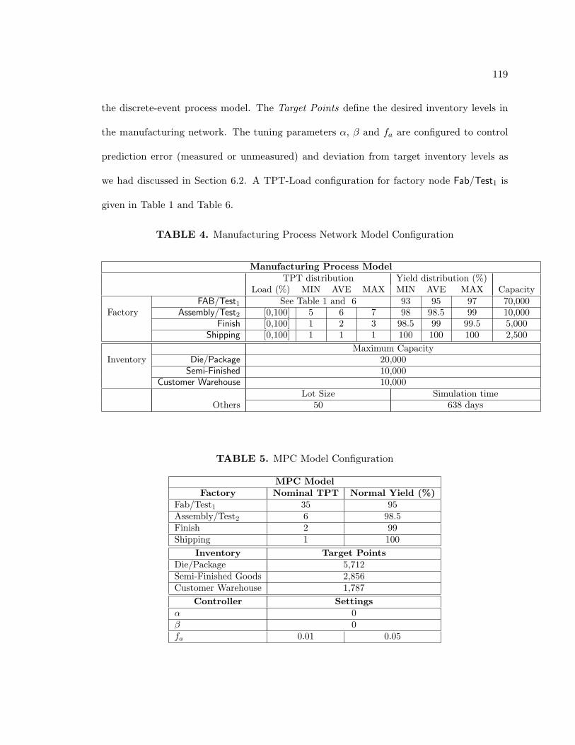
119
the discrete-event process model. The Target Points define the desired inventory levels in
the manufacturing network. The tuning parameters α, β and fa are configured to control
prediction error (measured or unmeasured) and deviation from target inventory levels as
we had discussed in Section 6.2. A TPT-Load configuration for factory node Fab/Test1 is
given in Table 1 and Table 6.
TABLE 4. Manufacturing Process Network Model Configuration
Manufacturing Process ModelTPT distribution Yield distribution (%)
Load (%) MIN AVE MAX MIN AVE MAX CapacityFAB/Test1 See Table 1 and 6 93 95 97 70,000
Factory Assembly/Test2 [0,100] 5 6 7 98 98.5 99 10,000Finish [0,100] 1 2 3 98.5 99 99.5 5,000
Shipping [0,100] 1 1 1 100 100 100 2,500Maximum Capacity
Inventory Die/Package 20,000Semi-Finished 10,000
Customer Warehouse 10,000Lot Size Simulation time
Others 50 638 days
TABLE 5. MPC Model Configuration
MPC ModelFactory Nominal TPT Normal Yield (%)
Fab/Test1 35 95Assembly/Test2 6 98.5Finish 2 99Shipping 1 100
Inventory Target PointsDie/Package 5,712Semi-Finished Goods 2,856Customer Warehouse 1,787
Controller Settingsα 0β 0fa 0.01 0.05
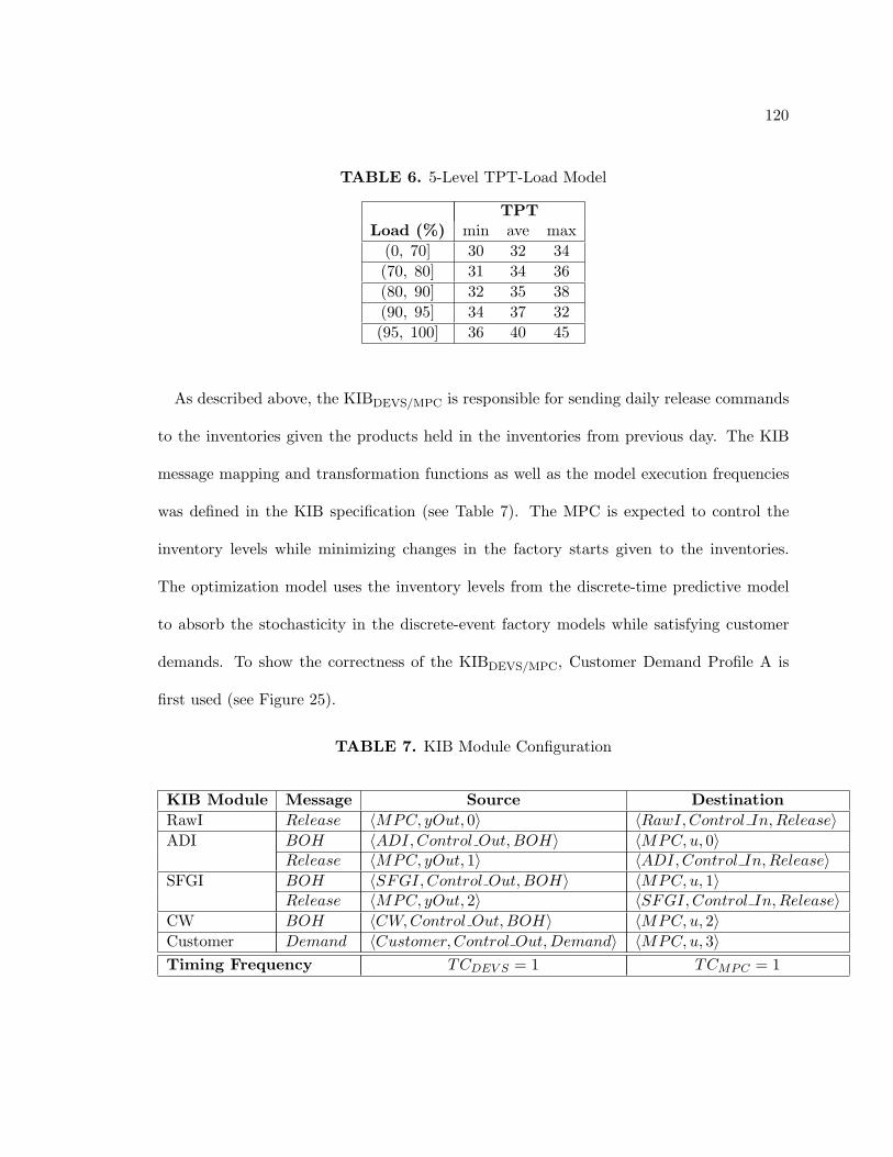
120
TABLE 6. 5-Level TPT-Load Model
TPTLoad (%) min ave max
(0, 70] 30 32 34(70, 80] 31 34 36(80, 90] 32 35 38(90, 95] 34 37 32(95, 100] 36 40 45
As described above, the KIBDEVS/MPC is responsible for sending daily release commands
to the inventories given the products held in the inventories from previous day. The KIB
message mapping and transformation functions as well as the model execution frequencies
was defined in the KIB specification (see Table 7). The MPC is expected to control the
inventory levels while minimizing changes in the factory starts given to the inventories.
The optimization model uses the inventory levels from the discrete-time predictive model
to absorb the stochasticity in the discrete-event factory models while satisfying customer
demands. To show the correctness of the KIBDEVS/MPC, Customer Demand Profile A is
first used (see Figure 25).
TABLE 7. KIB Module Configuration
KIB Module Message Source DestinationRawI Release 〈MPC, yOut, 0〉 〈RawI,Control In,Release〉ADI BOH 〈ADI, Control Out, BOH〉 〈MPC, u, 0〉
Release 〈MPC, yOut, 1〉 〈ADI,Control In, Release〉SFGI BOH 〈SFGI, Control Out,BOH〉 〈MPC, u, 1〉
Release 〈MPC, yOut, 2〉 〈SFGI, Control In,Release〉CW BOH 〈CW,Control Out, BOH〉 〈MPC, u, 2〉Customer Demand 〈Customer,Control Out, Demand〉 〈MPC, u, 3〉Timing Frequency TCDEV S = 1 TCMPC = 1
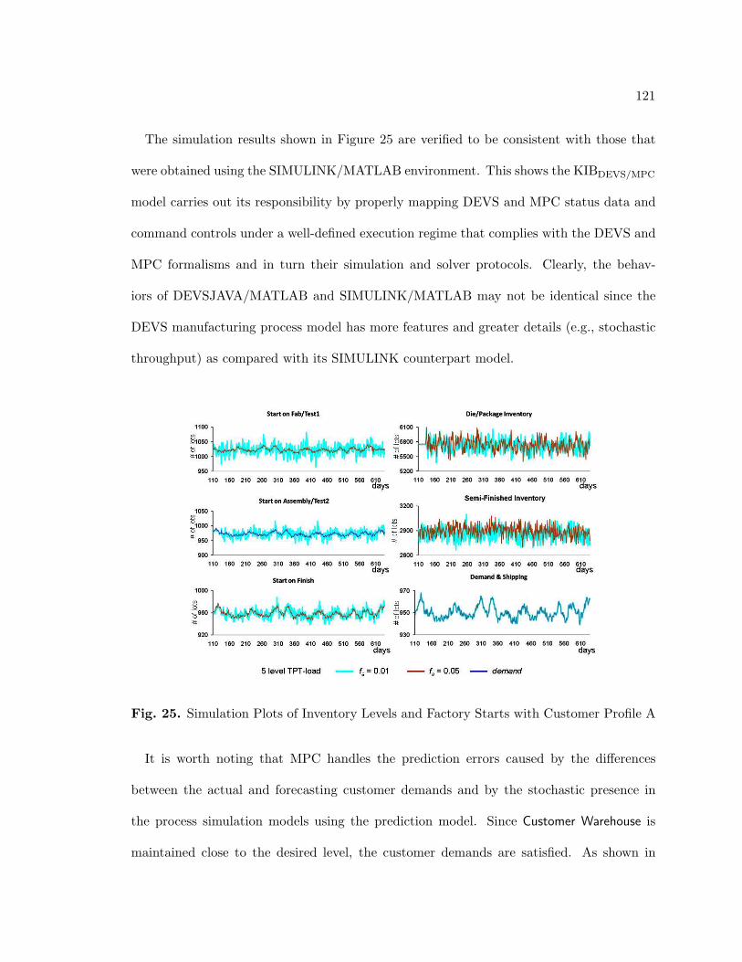
121
The simulation results shown in Figure 25 are verified to be consistent with those that
were obtained using the SIMULINK/MATLAB environment. This shows the KIBDEVS/MPC
model carries out its responsibility by properly mapping DEVS and MPC status data and
command controls under a well-defined execution regime that complies with the DEVS and
MPC formalisms and in turn their simulation and solver protocols. Clearly, the behav-
iors of DEVSJAVA/MATLAB and SIMULINK/MATLAB may not be identical since the
DEVS manufacturing process model has more features and greater details (e.g., stochastic
throughput) as compared with its SIMULINK counterpart model.
Fig. 25. Simulation Plots of Inventory Levels and Factory Starts with Customer Profile A
It is worth noting that MPC handles the prediction errors caused by the differences
between the actual and forecasting customer demands and by the stochastic presence in
the process simulation models using the prediction model. Since Customer Warehouse is
maintained close to the desired level, the customer demands are satisfied. As shown in
122
Figure 25, fine-grain control of factory starts can be achieved with a small filter gain (fa).
While a filter gain greater than zero is necessary for feedback control, its value needs to be
determined judicially in order to have an acceptable tradeoff between fast responses to the
changes in the process models and preventing potential instability caused by large changes
in factory starts. For example, the simulation results show the average starts for Fab/Test1
varies only 0.2% when fa changes from 0.01 to 0.05. However, the maximum starts increases
by 255% if is changed from 0.01 to 0.05.
Customer Demands Profile B is given to the hybrid environment to evaluate the robust-
ness of the MPC model in response to sharp changes in customer demand. To study the
robustness of the MPC, it can be subjected to significant nonlinearity and stochasticity.
For example, the customer demand can be changed by 50% and thus cause significant non-
linearity in Fab/Test1 due to the TPT-load relationship. In this experiment, the DEVS,
MPC, and KIBDEVS/MPC models are configured as shown in Table 4 with some exceptions.
Factory models are configured with larger capacities in order to handle large increase in cus-
tomer demand —i.e., CFab/Test1 = 70, 000, Cassembly/Test2 = 10, 000, and CFinish = 5, 000.
The choice of these levels is considered appropriate [38, 96]. The simulation results are
shown in Figure 26, Figure 27, and Figure 28. As shown in the results, the Die/Package
inventory undergoes transient dynamics due to the dramatic change in TPT in the up-
stream Fab/Test1 factory mode given a 3-level TPT-load function. Ideally, when Fab/Test1
maintains its load within specific range (e.g., Load ∈ [72%, 76%]), the average TPT can be
kept at the average of 35 days in the process simulation model. Accordingly, such average
TPT value is consistent with the corresponding nominal TPT parameter configured in MPC
model. However, due to the significant increase in customer demand, starts on Fab/Test1,
which is determined by the MPC model, is increased. This in turn results in increase load
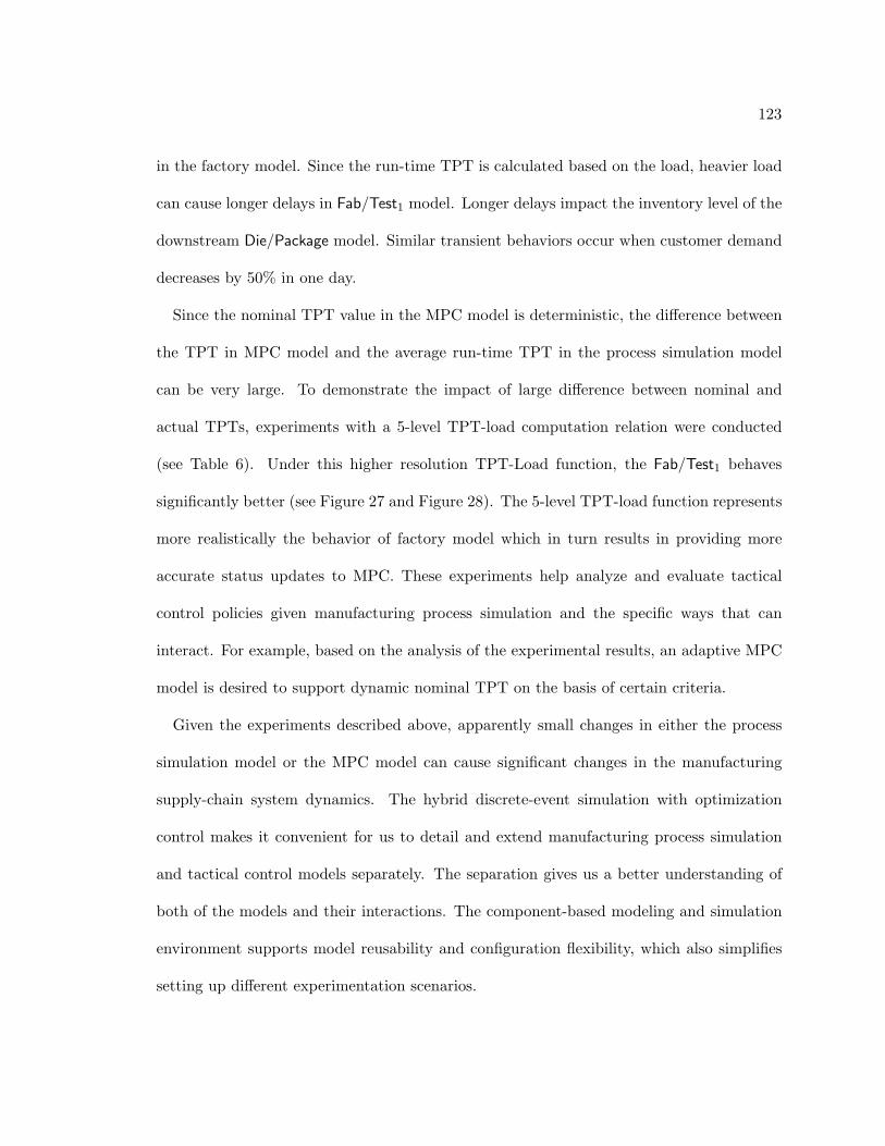
123
in the factory model. Since the run-time TPT is calculated based on the load, heavier load
can cause longer delays in Fab/Test1 model. Longer delays impact the inventory level of the
downstream Die/Package model. Similar transient behaviors occur when customer demand
decreases by 50% in one day.
Since the nominal TPT value in the MPC model is deterministic, the difference between
the TPT in MPC model and the average run-time TPT in the process simulation model
can be very large. To demonstrate the impact of large difference between nominal and
actual TPTs, experiments with a 5-level TPT-load computation relation were conducted
(see Table 6). Under this higher resolution TPT-Load function, the Fab/Test1 behaves
significantly better (see Figure 27 and Figure 28). The 5-level TPT-load function represents
more realistically the behavior of factory model which in turn results in providing more
accurate status updates to MPC. These experiments help analyze and evaluate tactical
control policies given manufacturing process simulation and the specific ways that can
interact. For example, based on the analysis of the experimental results, an adaptive MPC
model is desired to support dynamic nominal TPT on the basis of certain criteria.
Given the experiments described above, apparently small changes in either the process
simulation model or the MPC model can cause significant changes in the manufacturing
supply-chain system dynamics. The hybrid discrete-event simulation with optimization
control makes it convenient for us to detail and extend manufacturing process simulation
and tactical control models separately. The separation gives us a better understanding of
both of the models and their interactions. The component-based modeling and simulation
environment supports model reusability and configuration flexibility, which also simplifies
setting up different experimentation scenarios.
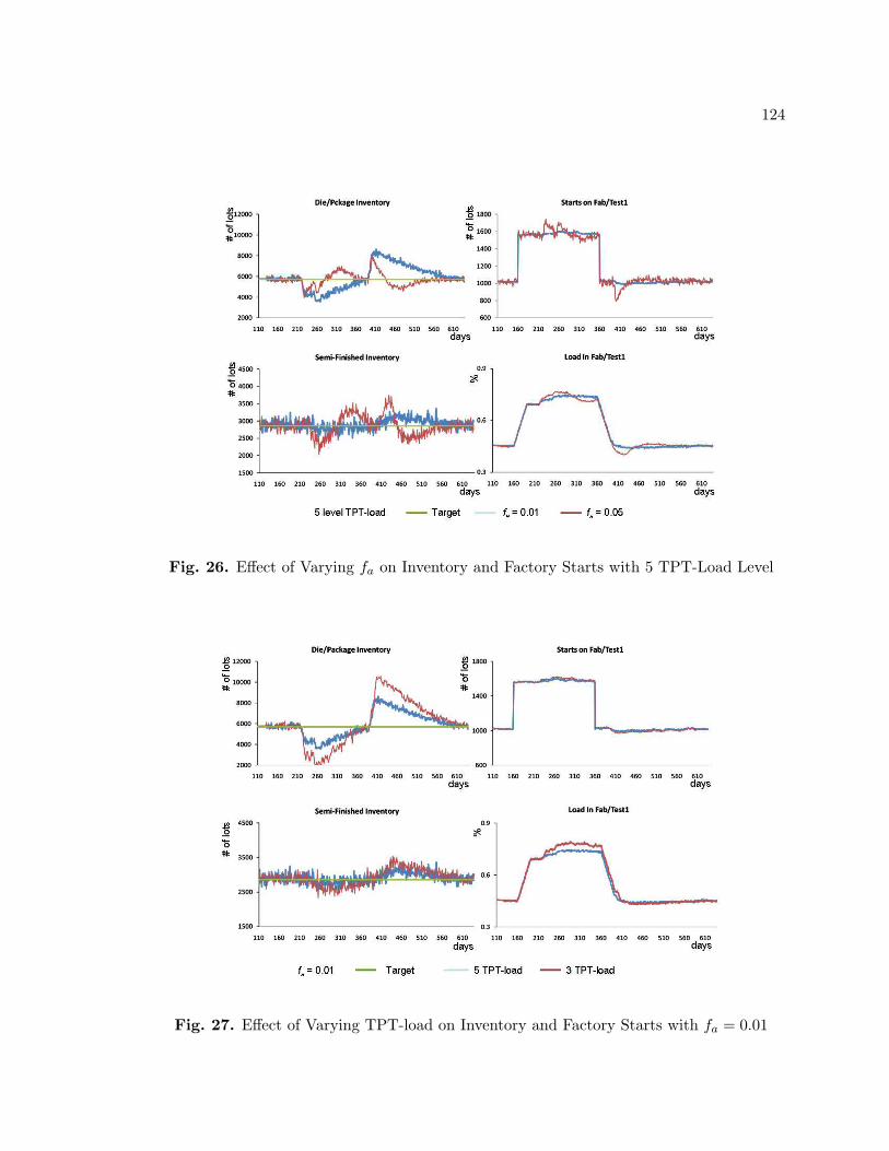
124
Fig. 26. Effect of Varying fa on Inventory and Factory Starts with 5 TPT-Load Level
Fig. 27. Effect of Varying TPT-load on Inventory and Factory Starts with fa = 0.01
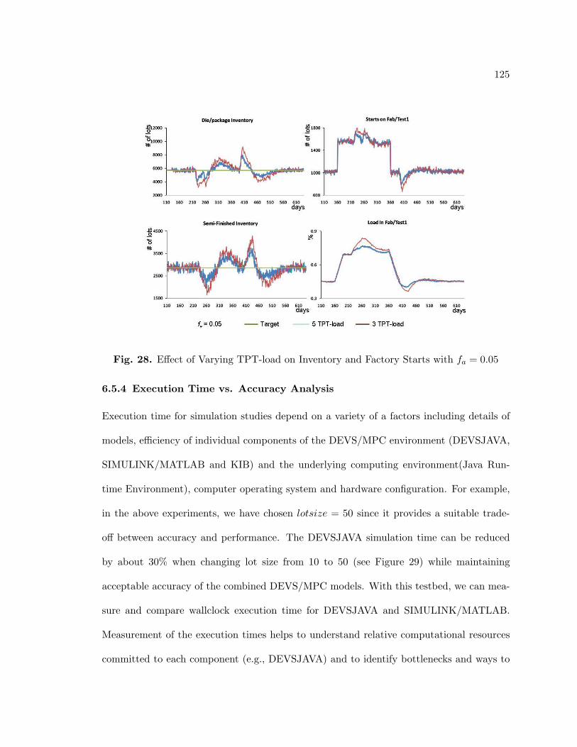
125
Fig. 28. Effect of Varying TPT-load on Inventory and Factory Starts with fa = 0.05
6.5.4 Execution Time vs. Accuracy Analysis
Execution time for simulation studies depend on a variety of a factors including details of
models, efficiency of individual components of the DEVS/MPC environment (DEVSJAVA,
SIMULINK/MATLAB and KIB) and the underlying computing environment(Java Run-
time Environment), computer operating system and hardware configuration. For example,
in the above experiments, we have chosen lotsize = 50 since it provides a suitable trade-
off between accuracy and performance. The DEVSJAVA simulation time can be reduced
by about 30% when changing lot size from 10 to 50 (see Figure 29) while maintaining
acceptable accuracy of the combined DEVS/MPC models. With this testbed, we can mea-
sure and compare wallclock execution time for DEVSJAVA and SIMULINK/MATLAB.
Measurement of the execution times helps to understand relative computational resources
committed to each component (e.g., DEVSJAVA) and to identify bottlenecks and ways to
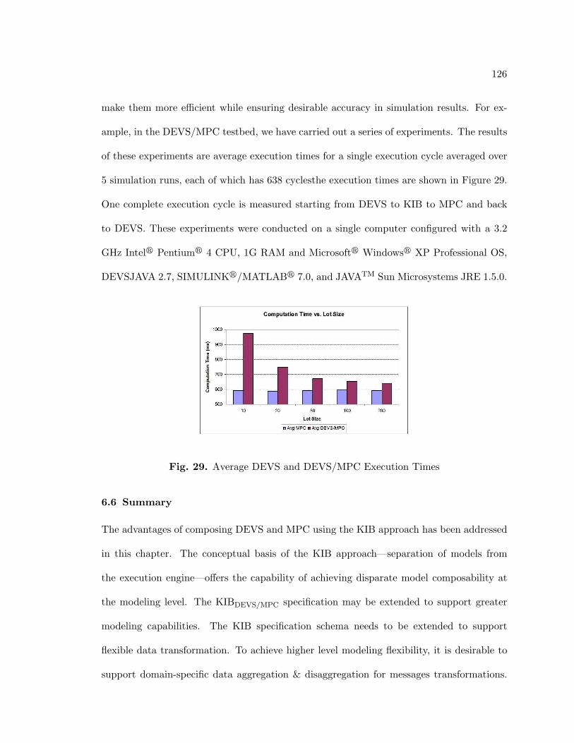
126
make them more efficient while ensuring desirable accuracy in simulation results. For ex-
ample, in the DEVS/MPC testbed, we have carried out a series of experiments. The results
of these experiments are average execution times for a single execution cycle averaged over
5 simulation runs, each of which has 638 cyclesthe execution times are shown in Figure 29.
One complete execution cycle is measured starting from DEVS to KIB to MPC and back
to DEVS. These experiments were conducted on a single computer configured with a 3.2
GHz Intelr Pentiumr 4 CPU, 1G RAM and Microsoftr Windowsr XP Professional OS,
DEVSJAVA 2.7, SIMULINKr/MATLABr 7.0, and JAVATM Sun Microsystems JRE 1.5.0.
Fig. 29. Average DEVS and DEVS/MPC Execution Times
6.6 Summary
The advantages of composing DEVS and MPC using the KIB approach has been addressed
in this chapter. The conceptual basis of the KIB approach—separation of models from
the execution engine—offers the capability of achieving disparate model composability at
the modeling level. The KIBDEVS/MPC specification may be extended to support greater
modeling capabilities. The KIB specification schema needs to be extended to support
flexible data transformation. To achieve higher level modeling flexibility, it is desirable to
support domain-specific data aggregation & disaggregation for messages transformations.

127
The KIB specification also needs to support flexible time synchronization between DEVS
and MPC model executions. The KIBDEVS/LP configurable execution control [28, 25] can
be adopted for KIBDEVS/MPC. Furthermore, concurrent execution scheme plays a key role
when there exist more than one control sub-system. In the following chapter, an approach
is developed to support parallel execution of MPC and LP with respect to DEVS.
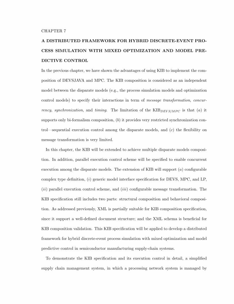
CHAPTER 7
A DISTRIBUTED FRAMEWORK FOR HYBRID DISCRETE-EVENT PRO-
CESS SIMULATION WITH MIXED OPTIMIZATION AND MODEL PRE-
DICTIVE CONTROL
In the previous chapter, we have shown the advantages of using KIB to implement the com-
position of DEVSJAVA and MPC. The KIB composition is considered as an independent
model between the disparate models (e.g., the process simulation models and optimization
control models) to specify their interactions in term of message transformation, concur-
rency, synchronization, and timing. The limitation of the KIBDEV S/MPC is that (a) it
supports only bi-formalism composition, (b) it provides very restricted synchronization con-
trol—sequential execution control among the disparate models, and (c) the flexibility on
message transformation is very limited.
In this chapter, the KIB will be extended to achieve multiple disparate models composi-
tion. In addition, parallel execution control scheme will be specified to enable concurrent
execution among the disparate models. The extension of KIB will support (a) configurable
complex type definition, (i) generic model interface specification for DEVS, MPC, and LP,
(ii) parallel execution control scheme, and (iii) configurable message transformation. The
KIB specification still includes two parts: structural composition and behavioral composi-
tion. As addressed previously, XML is partially suitable for KIB composition specification,
since it support a well-defined document structure; and the XML schema is beneficial for
KIB composition validation. This KIB specification will be applied to develop a distributed
framework for hybrid discrete-event process simulation with mixed optimization and model
predictive control in semiconductor manufacturing supply-chain systems.
To demonstrate the KIB specification and its execution control in detail, a simplified
supply chain management system, in which a processing network system is managed by
129
two levels of decision controls, will be used as an example. The processing network sub-
system consists of a factory (Factory), an inventory (Inventory), and two customer centers
(CustomerA and CustomerB). Two decision sub-systems—a tactical controller (Controller)
and a strategic planner (Planner) provide multi-level decision controls against the dynam-
ics of the processing network. Given the distinguished features of each subsystem, a set
of supply chain process models—Factory, Inventory, CustomerA, and CustomerB —simulate
the daily dynamics of the processing network using discrete event modeling and simulation
methodology (modeled in DEVSJAVA), whereas the Controller and Planner generate short-
term (daily) tactical control and long-term (weekly) strategic planning using MPC technol-
ogy (implemented in MATLAB) and LP optimization technology (developed in CPLEX)
respectively. The interactions among the disparate models are described in Figure 30.
Fig. 30. Combined Supply Chain Manufacturing System with Tactical Controller andStrategic Planner
We assume that two products (Prod1 and Prod2) are produced from Factory to Inventory.
The manufacturing Inventory provides the Controller and Planner with daily and weekly in-
130
ventory BOH respectively. The demand from the two customer centers (CustomerA and
CustomerB) to the Planner is assumed to be an estimation of next 14 days of customer
demands. In turn, the Planner computes and sends weekly targeting inventory level refer-
ences to the Controller, whereas the Controller computes and sends daily inventory release
commands to the Inventory.
7.1 KIB Structural Composition Specification
Disparate modeling formalisms generally present distinct specification on model structure.
The interface structure for a DEVS model can be described in the form of 〈model, port,
data〉. The interface structure for an optimization model or MPC model, on the other hand,
is generally numerical variables (X = ∪xi, xi ∈ <). In addition, the modeling languages, or
the modeling environments can support customized data type definition to facilitate vari-
able specification, which can consequently have a great impact on the interface structures.
Therefore, the KIB specification must account for (i) the distinct syntax and semantics
among the disparate modeling structures specified in the modeling formalism, (ii) data
transformation among different data types, and (iii) domain-specific knowledge transfor-
mation.
The principles of specifying the structural composition include
� It needs to capture the interface specialties of each modeling formalism involved in
the interactions.
� The interactions between the disparate models are essentially related to one or more
models representing a specific entity in the system. Such entities can be treated as
independent models within KIB.
131
� Data payload held within the model message need to be considered explicitly since the
data transformed among disparate models may be in different forms although they
are carrying the same domain-specific knowledge.
The structural specification of KIBDEVS/MPC/LP needs to consist of DEVS interface, LP
interface, MPC interface, KIB model, and complex data type specification.
7.1.1 DEVS Model Interface Specification
The messages to/from the DEVS interface are associated with a DEVS model and the
port(s). The messages that are used to interact with non-DEVS models need to be specified
in the KIB specification. For example, in the Figure 30, Inventory has an interaction with
both Controller and Planner. It receives Release messages from Controller and it provides
BOH to both Controller and Planner. The following is the DEVS interface specification of
Inventory model.
<DESModule name="inventory"><InPort name="Control_In">
<Variable name="Release" type="DESProduction" size="n"/></InPort><OutPort name="Control_Out">
<Variable name="BOH" type="DESProduction" size="n" /></OutPort>
</DESModule>
A collection element DESModules is used to enclose all the DEVS simulation models.
Each DEVS simulation model that participates in the disparate model interaction is spec-
ified in the element DESModule. The attribute name in the element DESModule is re-
quired and should be unique in the KIB specification. The ports in DEVS model are uni-
directional—input ports (InPort) or output ports (OutPort). Special input/output ports
(Control In and Control Out) have been specified in DEVS to play a special role in the
model interaction with non-DEVS components. Therefore, the attribute name in the In-
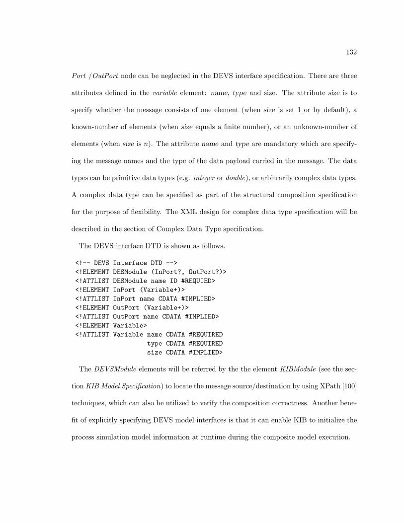
132
Port /OutPort node can be neglected in the DEVS interface specification. There are three
attributes defined in the variable element: name, type and size. The attribute size is to
specify whether the message consists of one element (when size is set 1 or by default), a
known-number of elements (when size equals a finite number), or an unknown-number of
elements (when size is n). The attribute name and type are mandatory which are specify-
ing the message names and the type of the data payload carried in the message. The data
types can be primitive data types (e.g. integer or double), or arbitrarily complex data types.
A complex data type can be specified as part of the structural composition specification
for the purpose of flexibility. The XML design for complex data type specification will be
described in the section of Complex Data Type specification.
The DEVS interface DTD is shown as follows.
<!-- DEVS Interface DTD --><!ELEMENT DESModule (InPort?, OutPort?)><!ATTLIST DESModule name ID #REQUIED><!ELEMENT InPort (Variable+)><!ATTLIST InPort name CDATA #IMPLIED><!ELEMENT OutPort (Variable+)><!ATTLIST OutPort name CDATA #IMPLIED><!ELEMENT Variable><!ATTLIST Variable name CDATA #REQUIRED
type CDATA #REQUIREDsize CDATA #IMPLIED>
The DEVSModule elements will be referred by the the element KIBModule (see the sec-
tion KIB Model Specification) to locate the message source/destination by using XPath [100]
techniques, which can also be utilized to verify the composition correctness. Another bene-
fit of explicitly specifying DEVS model interfaces is that it can enable KIB to initialize the
process simulation model information at runtime during the composite model execution.
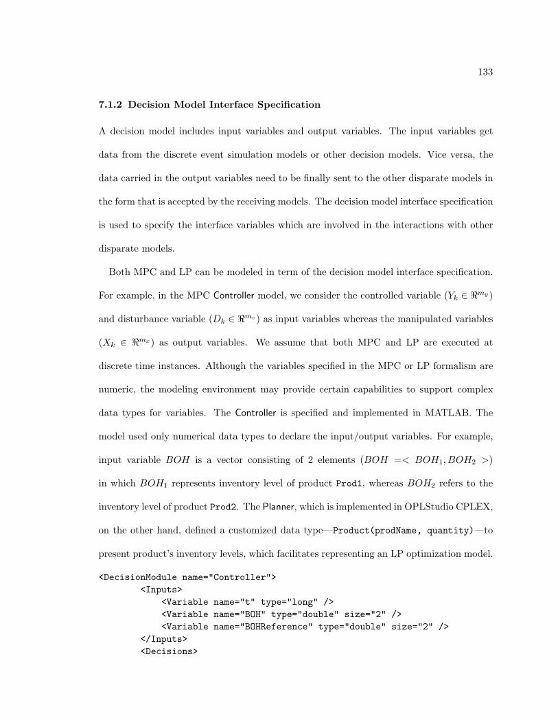
133
7.1.2 Decision Model Interface Specification
A decision model includes input variables and output variables. The input variables get
data from the discrete event simulation models or other decision models. Vice versa, the
data carried in the output variables need to be finally sent to the other disparate models in
the form that is accepted by the receiving models. The decision model interface specification
is used to specify the interface variables which are involved in the interactions with other
disparate models.
Both MPC and LP can be modeled in term of the decision model interface specification.
For example, in the MPC Controller model, we consider the controlled variable (Yk ∈ <my)
and disturbance variable (Dk ∈ <mv) as input variables whereas the manipulated variables
(Xk ∈ <mx) as output variables. We assume that both MPC and LP are executed at
discrete time instances. Although the variables specified in the MPC or LP formalism are
numeric, the modeling environment may provide certain capabilities to support complex
data types for variables. The Controller is specified and implemented in MATLAB. The
model used only numerical data types to declare the input/output variables. For example,
input variable BOH is a vector consisting of 2 elements (BOH =< BOH1, BOH2 >)
in which BOH1 represents inventory level of product Prod1, whereas BOH2 refers to the
inventory level of product Prod2. The Planner, which is implemented in OPLStudio CPLEX,
on the other hand, defined a customized data type—Product(prodName, quantity)—to
present product’s inventory levels, which facilitates representing an LP optimization model.
<DecisionModule name="Controller"><Inputs>
<Variable name="t" type="long" /><Variable name="BOH" type="double" size="2" /><Variable name="BOHReference" type="double" size="2" />
</Inputs><Decisions>
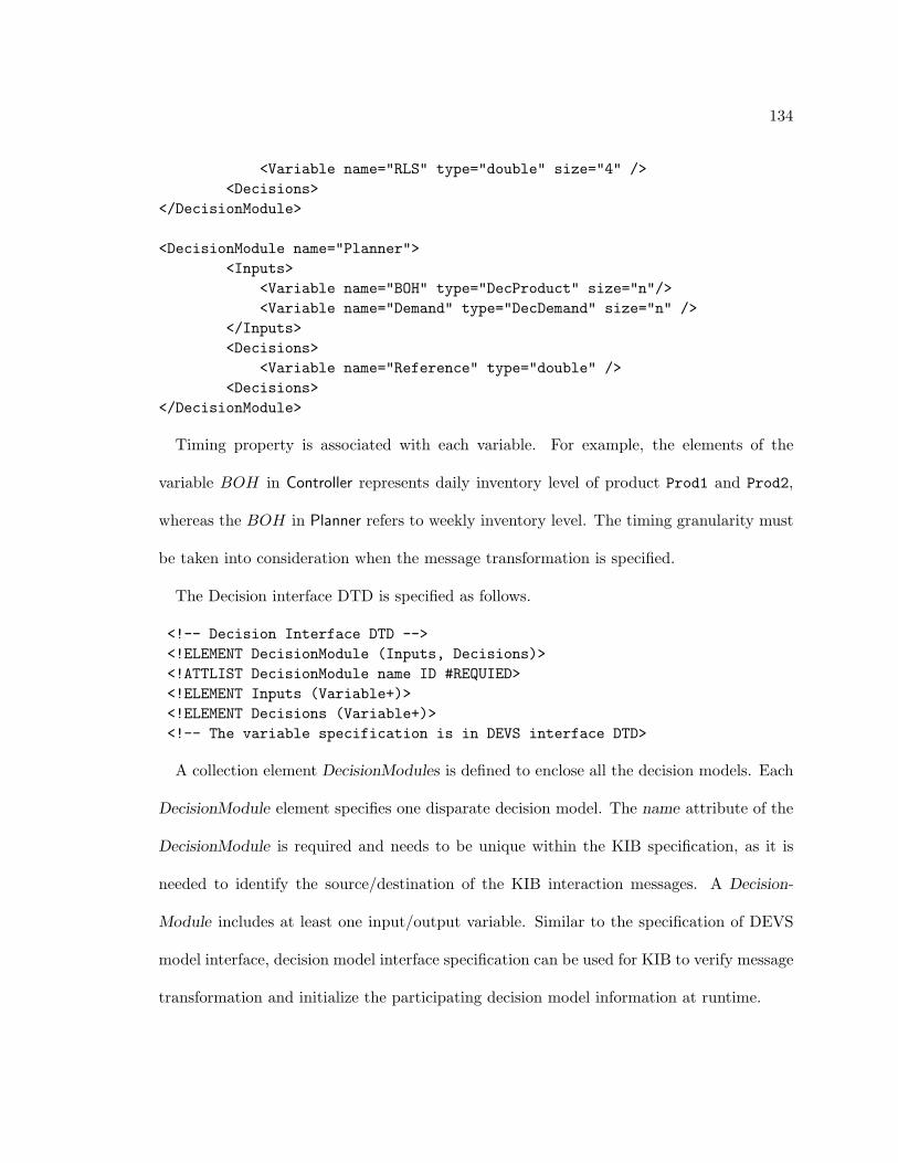
134
<Variable name="RLS" type="double" size="4" /><Decisions>
</DecisionModule>
<DecisionModule name="Planner"><Inputs>
<Variable name="BOH" type="DecProduct" size="n"/><Variable name="Demand" type="DecDemand" size="n" />
</Inputs><Decisions>
<Variable name="Reference" type="double" /><Decisions>
</DecisionModule>
Timing property is associated with each variable. For example, the elements of the
variable BOH in Controller represents daily inventory level of product Prod1 and Prod2,
whereas the BOH in Planner refers to weekly inventory level. The timing granularity must
be taken into consideration when the message transformation is specified.
The Decision interface DTD is specified as follows.
<!-- Decision Interface DTD --><!ELEMENT DecisionModule (Inputs, Decisions)><!ATTLIST DecisionModule name ID #REQUIED><!ELEMENT Inputs (Variable+)><!ELEMENT Decisions (Variable+)><!-- The variable specification is in DEVS interface DTD>
A collection element DecisionModules is defined to enclose all the decision models. Each
DecisionModule element specifies one disparate decision model. The name attribute of the
DecisionModule is required and needs to be unique within the KIB specification, as it is
needed to identify the source/destination of the KIB interaction messages. A Decision-
Module includes at least one input/output variable. Similar to the specification of DEVS
model interface, decision model interface specification can be used for KIB to verify message
transformation and initialize the participating decision model information at runtime.
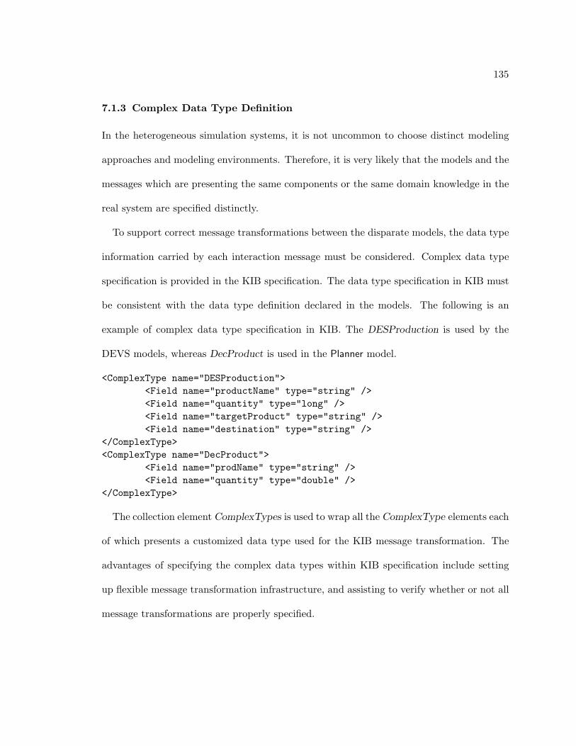
135
7.1.3 Complex Data Type Definition
In the heterogeneous simulation systems, it is not uncommon to choose distinct modeling
approaches and modeling environments. Therefore, it is very likely that the models and the
messages which are presenting the same components or the same domain knowledge in the
real system are specified distinctly.
To support correct message transformations between the disparate models, the data type
information carried by each interaction message must be considered. Complex data type
specification is provided in the KIB specification. The data type specification in KIB must
be consistent with the data type definition declared in the models. The following is an
example of complex data type specification in KIB. The DESProduction is used by the
DEVS models, whereas DecProduct is used in the Planner model.
<ComplexType name="DESProduction"><Field name="productName" type="string" /><Field name="quantity" type="long" /><Field name="targetProduct" type="string" /><Field name="destination" type="string" />
</ComplexType><ComplexType name="DecProduct">
<Field name="prodName" type="string" /><Field name="quantity" type="double" />
</ComplexType>
The collection element ComplexTypes is used to wrap all the ComplexType elements each
of which presents a customized data type used for the KIB message transformation. The
advantages of specifying the complex data types within KIB specification include setting
up flexible message transformation infrastructure, and assisting to verify whether or not all
message transformations are properly specified.
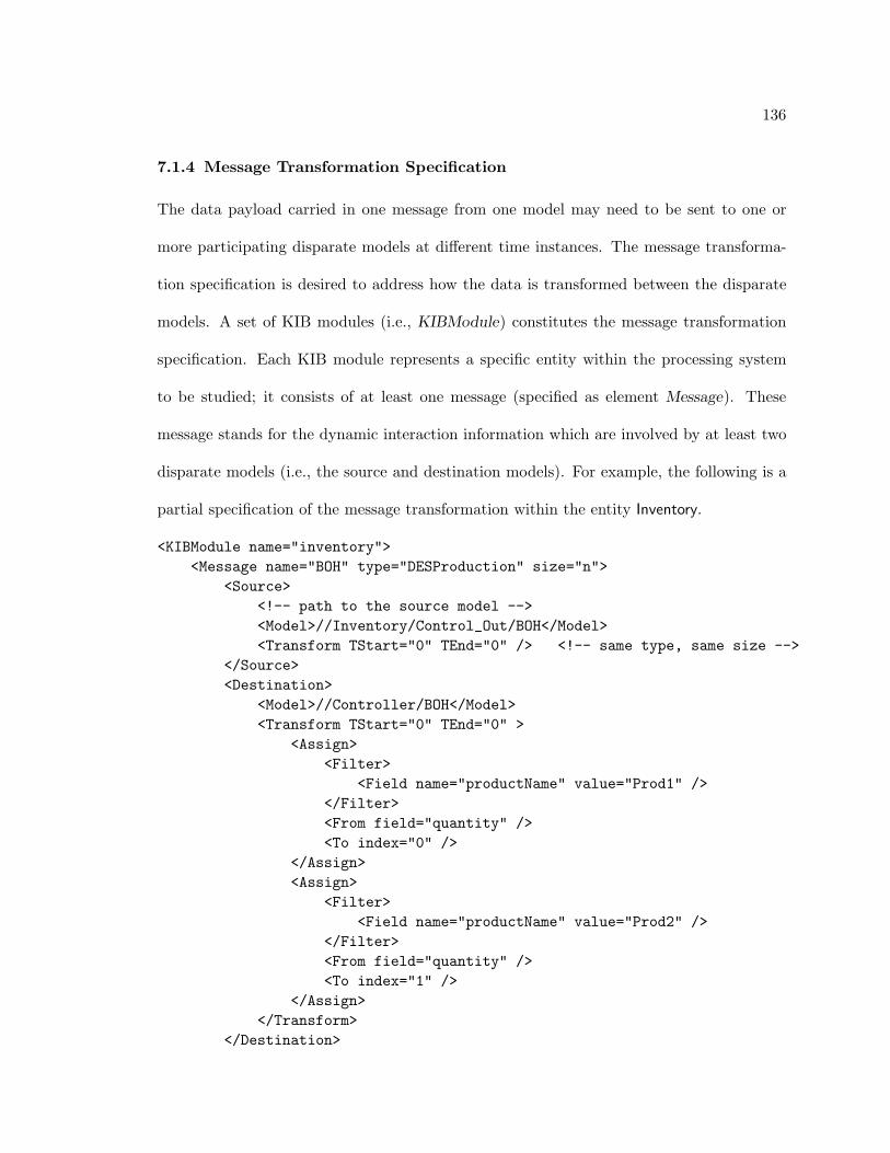
136
7.1.4 Message Transformation Specification
The data payload carried in one message from one model may need to be sent to one or
more participating disparate models at different time instances. The message transforma-
tion specification is desired to address how the data is transformed between the disparate
models. A set of KIB modules (i.e., KIBModule) constitutes the message transformation
specification. Each KIB module represents a specific entity within the processing system
to be studied; it consists of at least one message (specified as element Message). These
message stands for the dynamic interaction information which are involved by at least two
disparate models (i.e., the source and destination models). For example, the following is a
partial specification of the message transformation within the entity Inventory.
<KIBModule name="inventory"><Message name="BOH" type="DESProduction" size="n">
<Source><!-- path to the source model --><Model>//Inventory/Control_Out/BOH</Model><Transform TStart="0" TEnd="0" /> <!-- same type, same size -->
</Source><Destination>
<Model>//Controller/BOH</Model><Transform TStart="0" TEnd="0" >
<Assign><Filter>
<Field name="productName" value="Prod1" /></Filter><From field="quantity" /><To index="0" />
</Assign><Assign>
<Filter><Field name="productName" value="Prod2" />
</Filter><From field="quantity" /><To index="1" />
</Assign></Transform>
</Destination>
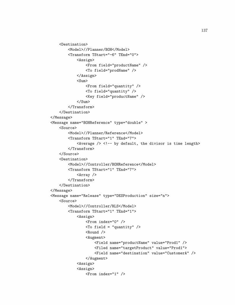
137
<Destination><Model>//Planner/BOH</Model><Transform TStart="-6" TEnd="0">
<Assign><From field="productName" /><To field="prodName" />
</Assign><Sum>
<From field="quantity" /><To field="quantity" /><Key field="productName" />
</Sum></Transform>
</Destination></Message><Message name="BOHReference" type="double" >
<Source><Model>//Planner/Reference</Model><Transform TStart="1" TEnd="7">
<Average /> <!-- by default, the divisor is time length></Transform>
</Source><Destination>
<Model>//Controller/BOHReference</Model><Transform TStart="1" TEnd="7">
<Array /></Transform>
</Destination></Message><Message name="Release" type="DESProduction" size="n">
<Source><Model>//Controller/RLS</Model><Transform TStart="1" TEnd="1">
<Assign><From index="0" /><To field = "quantity" /><Round /><Augment>
<Field name="productName" value="Prod1" /><Filed name="targetProduct" value="Prod1"><Field name="destination" value="CustomerA" />
</Augment><Assign><Assign>
<From index="1" />
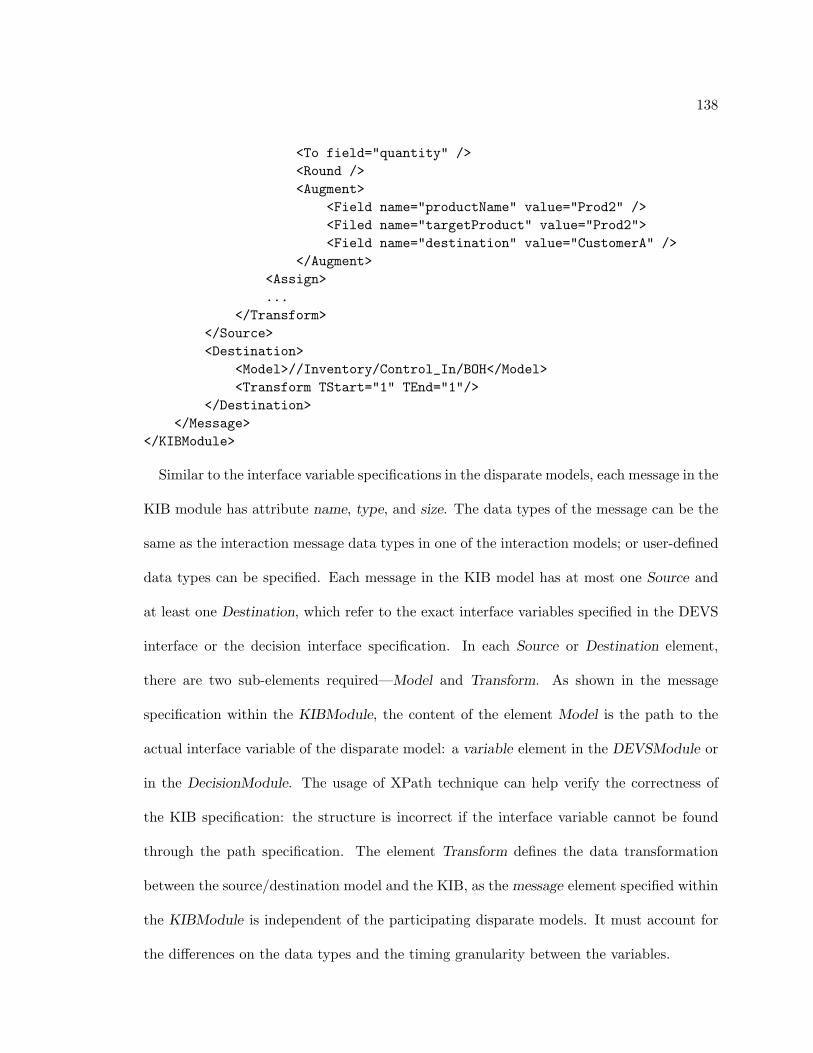
138
<To field="quantity" /><Round /><Augment>
<Field name="productName" value="Prod2" /><Filed name="targetProduct" value="Prod2"><Field name="destination" value="CustomerA" />
</Augment><Assign>...
</Transform></Source><Destination>
<Model>//Inventory/Control_In/BOH</Model><Transform TStart="1" TEnd="1"/>
</Destination></Message>
</KIBModule>
Similar to the interface variable specifications in the disparate models, each message in the
KIB module has attribute name, type, and size. The data types of the message can be the
same as the interaction message data types in one of the interaction models; or user-defined
data types can be specified. Each message in the KIB model has at most one Source and
at least one Destination, which refer to the exact interface variables specified in the DEVS
interface or the decision interface specification. In each Source or Destination element,
there are two sub-elements required—Model and Transform. As shown in the message
specification within the KIBModule, the content of the element Model is the path to the
actual interface variable of the disparate model: a variable element in the DEVSModule or
in the DecisionModule. The usage of XPath technique can help verify the correctness of
the KIB specification: the structure is incorrect if the interface variable cannot be found
through the path specification. The element Transform defines the data transformation
between the source/destination model and the KIB, as the message element specified within
the KIBModule is independent of the participating disparate models. It must account for
the differences on the data types and the timing granularity between the variables.
139
There exist a variety of possible data transformations among the interaction messages.
In KIB specification, a set of basic data transformations we considered can be categorized
as follows.
� Transformation between primitive data types.
– single-value to single-value, direct assignment or round operations such as Floor,
Ceiling or Round.
– multi-value to single-value, assignment of a specific value or aggregate operation
such as Sum, Min, Max, and Mean.
– single-value to multi-value, disaggregate operations such as dividing a single value
by a number to generate multiple values.
– multi-value to multi-value: direct array assignment.
� Transformation between a primitive data type and a complex data type
– knowledge reduction, assigning a field value of a variable with a complex data
type to a variable whose data type is primitive. This assignment may need to
satisfy certain criteria.
– knowledge augment, assigning a single value to a field of a variable with a complex
data type. The other fields of the variable may need to be assigned explicitly.
� Transformation between two different complex data types.
– assigning a field value of a variable with a complex data type to a field value of
a variable with another complex data types.
The different categories of data transformation operations can be combined to support
arbitrary complex data transformations. For instance, the data carried in the KIB model
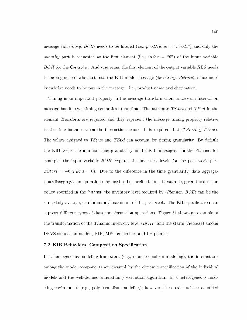
140
message 〈inventory, BOH〉 needs to be filtered (i.e., prodName = “Prod1”) and only the
quantity part is requested as the first element (i.e., index = “0”) of the input variable
BOH for the Controller. And vise versa, the first element of the output variable RLS needs
to be augmented when set into the KIB model message 〈inventory, Release〉, since more
knowledge needs to be put in the message—i.e., product name and destination.
Timing is an important property in the message transformation, since each interaction
message has its own timing semantics at runtime. The attribute TStart and TEnd in the
element Transform are required and they represent the message timing property relative
to the time instance when the interaction occurs. It is required that (TStart ≤ TEnd).
The values assigned to TStart and TEnd can account for timing granularity. By default
the KIB keeps the minimal time granularity in the KIB messages. In the Planner, for
example, the input variable BOH requires the inventory levels for the past week (i.e.,
TStart = −6, TEnd = 0). Due to the difference in the time granularity, data aggrega-
tion/disaggregation operation may need to be specified. In this example, given the decision
policy specified in the Planner, the inventory level required by 〈Planner, BOH〉 can be the
sum, daily-average, or minimum / maximum of the past week. The KIB specification can
support different types of data transformation operations. Figure 31 shows an example of
the transformation of the dynamic inventory level (BOH) and the starts (Release) among
DEVS simulation model , KIB, MPC controller, and LP planner.
7.2 KIB Behavioral Composition Specification
In a homogeneous modeling framework (e.g., mono-formalism modeling), the interactions
among the model components are ensured by the dynamic specification of the individual
models and the well-defined simulation / execution algorithm. In a heterogeneous mod-
eling environment (e.g., poly-formalism modeling), however, there exist neither a unified
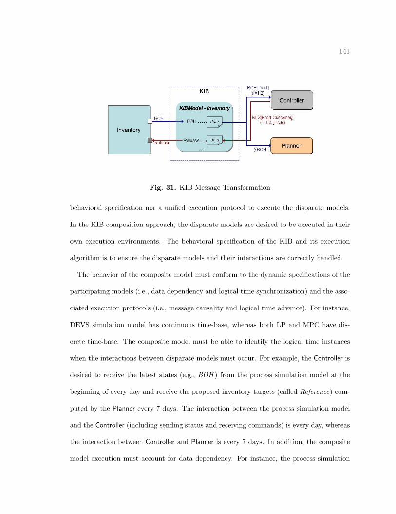
141
Fig. 31. KIB Message Transformation
behavioral specification nor a unified execution protocol to execute the disparate models.
In the KIB composition approach, the disparate models are desired to be executed in their
own execution environments. The behavioral specification of the KIB and its execution
algorithm is to ensure the disparate models and their interactions are correctly handled.
The behavior of the composite model must conform to the dynamic specifications of the
participating models (i.e., data dependency and logical time synchronization) and the asso-
ciated execution protocols (i.e., message causality and logical time advance). For instance,
DEVS simulation model has continuous time-base, whereas both LP and MPC have dis-
crete time-base. The composite model must be able to identify the logical time instances
when the interactions between disparate models must occur. For example, the Controller is
desired to receive the latest states (e.g., BOH ) from the process simulation model at the
beginning of every day and receive the proposed inventory targets (called Reference) com-
puted by the Planner every 7 days. The interaction between the process simulation model
and the Controller (including sending status and receiving commands) is every day, whereas
the interaction between Controller and Planner is every 7 days. In addition, the composite
model execution must account for data dependency. For instance, the process simulation
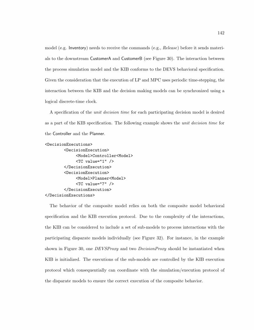
142
model (e.g. Inventory) needs to receive the commands (e.g., Release) before it sends materi-
als to the downstream CustomerA and CustomerB (see Figure 30). The interaction between
the process simulation model and the KIB conforms to the DEVS behavioral specification.
Given the consideration that the execution of LP and MPC uses periodic time-stepping, the
interaction between the KIB and the decision making models can be synchronized using a
logical discrete-time clock.
A specification of the unit decision time for each participating decision model is desired
as a part of the KIB specification. The following example shows the unit decision time for
the Controller and the Planner.
<DecisionExecutions><DecisionExecution>
<Model>Controller<Model><TC value="1" />
</DecisionExecution><DecisionExecution>
<Model>Planner<Model><TC value="7" />
</DecisionExecution></DecisionExecutions>
The behavior of the composite model relies on both the composite model behavioral
specification and the KIB execution protocol. Due to the complexity of the interactions,
the KIB can be considered to include a set of sub-models to process interactions with the
participating disparate models individually (see Figure 32). For instance, in the example
shown in Figure 30, one DEVSProxy and two DecisionProxy should be instantiated when
KIB is initialized. The executions of the sub-models are controlled by the KIB execution
protocol which consequentially can coordinate with the simulation/execution protocol of
the disparate models to ensure the correct execution of the composite behavior.
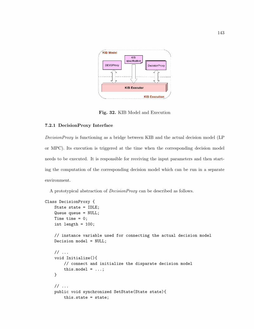
143
Fig. 32. KIB Model and Execution
7.2.1 DecisionProxy Interface
DecisionProxy is functioning as a bridge between KIB and the actual decision model (LP
or MPC). Its execution is triggered at the time when the corresponding decision model
needs to be executed. It is responsible for receiving the input parameters and then start-
ing the computation of the corresponding decision model which can be run in a separate
environment.
A prototypical abstraction of DecisionProxy can be described as follows.
Class DecisionProxy {State state = IDLE;Queue queue = NULL;Time time = 0;int length = 100;
// instance variable used for connecting the actual decision modelDecision model = NULL;
// ...void Initialize(){
// connect and initialize the disparate decision modelthis.model = ...;
}
// ...public void synchronized SetState(State state){
this.state = state;
144
}public void State synchronized GetState(){
return this.state;}
// trigger executionpublic void Execute(Time T){
this.time = T;this.SetState(BUSY);
}
// infinite loop to wait for messageprivate void run(){
while(1){
if (this.GetState() == BUSY){// get the transformed messageVariable InputVariable = NULL;while (InputVariable == NULL){
InputVariable =KIBTransformer.GetDecision(this, T);
wait(length);}// interact with the actual decision modelVariable OutputVariable = model.execute(InputVariable);// set computation resultKIBTransformer.UpdateDecision(OutputVariable, T);this.SetState(IDLE);
}}
}}
The method run in the DecisionProxy can be considered as part of the execution engine
within the KIB, since it is synchronizing with the KIBTransformer to get/set decision
model variables from/to the KIB.
7.2.2 DEVSProxy Interface
The DecisionProxy behaves passively — it is activated only when receiving input messages.
The DEVSProxy, on the contrary, is active — it sends the simulation update to the KIB
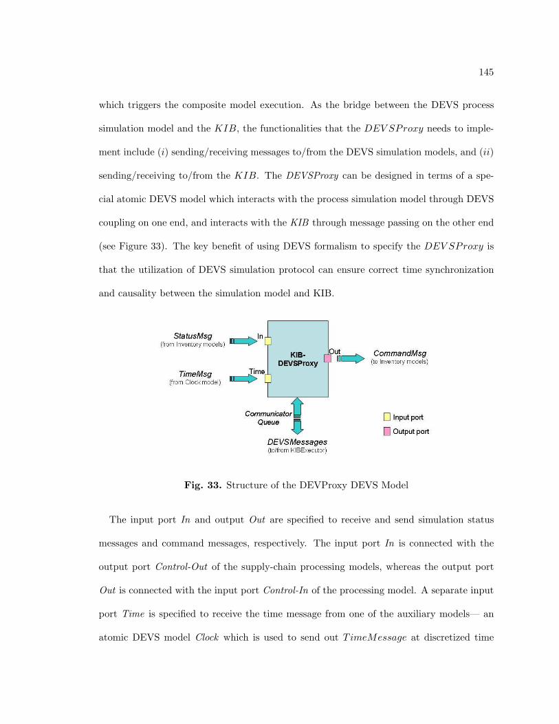
145
which triggers the composite model execution. As the bridge between the DEVS process
simulation model and the KIB, the functionalities that the DEV SProxy needs to imple-
ment include (i) sending/receiving messages to/from the DEVS simulation models, and (ii)
sending/receiving to/from the KIB. The DEVSProxy can be designed in terms of a spe-
cial atomic DEVS model which interacts with the process simulation model through DEVS
coupling on one end, and interacts with the KIB through message passing on the other end
(see Figure 33). The key benefit of using DEVS formalism to specify the DEV SProxy is
that the utilization of DEVS simulation protocol can ensure correct time synchronization
and causality between the simulation model and KIB.
Fig. 33. Structure of the DEVProxy DEVS Model
The input port In and output Out are specified to receive and send simulation status
messages and command messages, respectively. The input port In is connected with the
output port Control-Out of the supply-chain processing models, whereas the output port
Out is connected with the input port Control-In of the processing model. A separate input
port Time is specified to receive the time message from one of the auxiliary models— an
atomic DEVS model Clock which is used to send out TimeMessage at discretized time
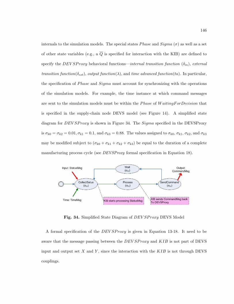
146
internals to the simulation models. The special states Phase and Sigma (σ) as well as a set
of other state variables (e.g., a Q is specified for interaction with the KIB) are defined to
specify the DEV SProxy behavioral functions—internal transition function (δin), external
transition function(δext), output function(λ), and time advanced function(ta). In particular,
the specification of Phase and Sigma must account for synchronizing with the operations
of the simulation models. For example, the time instance at which command messages
are sent to the simulation models must be within the Phase of WaitingForDecision that
is specified in the supply-chain node DEVS model (see Figure 14). A simplified state
diagram for DEV SProxy is shown in Figure 34. The Sigma specified in the DEVSProxy
is σk0 = σk2 = 0.01, σk1 = 0.1, and σk3 = 0.88. The values assigned to σk0, σk1, σk2, and σk3
may be modified subject to (σk0 + σk1 + σk2 + σk3) be equal to the duration of a complete
manufacturing process cycle (see DEVSProxy formal specification in Equation 18).
Fig. 34. Simplified State Diagram of DEV SProxy DEVS Model
A formal specification of the DEV SProxy is given in Equation 13-18. It need to be
aware that the message passing between the DEV SProxy and KIB is not part of DEVS
input and output set X and Y , since the interaction with the KIB is not through DEVS
couplings.
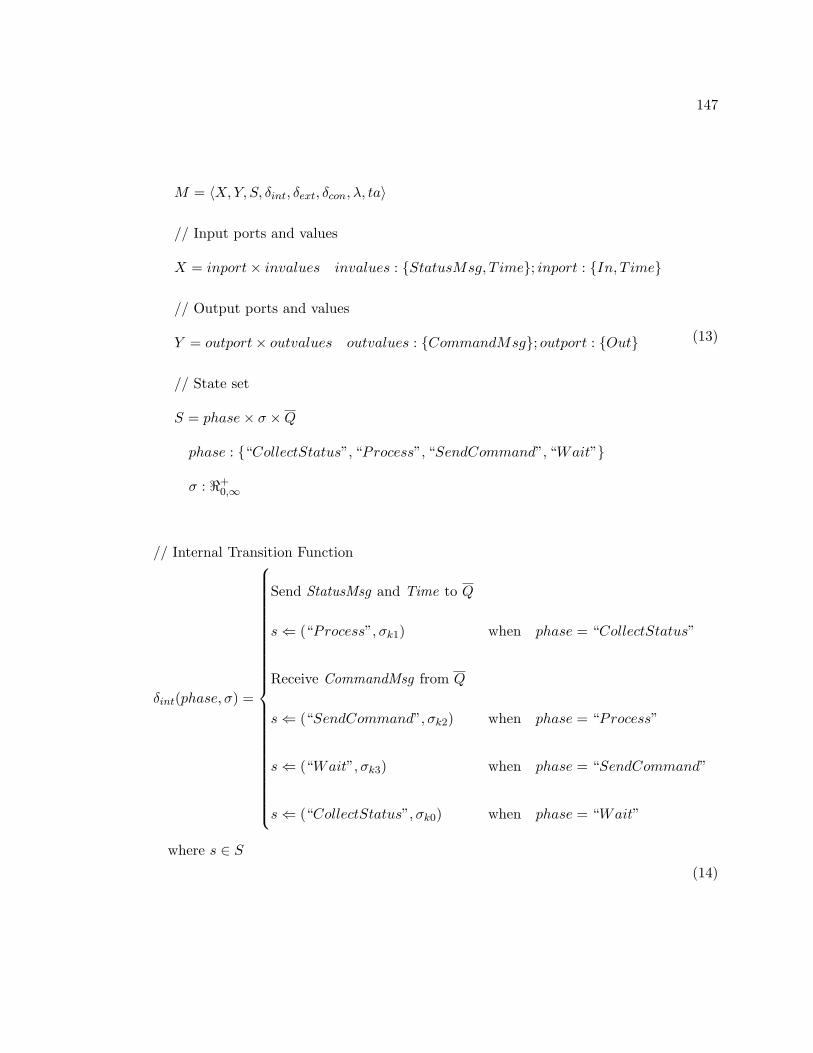
147
M = 〈X, Y, S, δint, δext, δcon, λ, ta〉
// Input ports and values
X = inport× invalues invalues : {StatusMsg, T ime}; inport : {In, T ime}
// Output ports and values
Y = outport× outvalues outvalues : {CommandMsg}; outport : {Out}
// State set
S = phase× σ ×Q
phase : {“CollectStatus”, “Process”, “SendCommand”, “Wait”}
σ : <+0,∞
(13)
// Internal Transition Function
δint(phase, σ) =
Send StatusMsg and Time to Q
s ⇐ (“Process”, σk1) when phase = “CollectStatus”
Receive CommandMsg from Q
s ⇐ (“SendCommand”, σk2) when phase = “Process”
s ⇐ (“Wait”, σk3) when phase = “SendCommand”
s ⇐ (“CollectStatus”, σk0) when phase = “Wait”
where s ∈ S
(14)
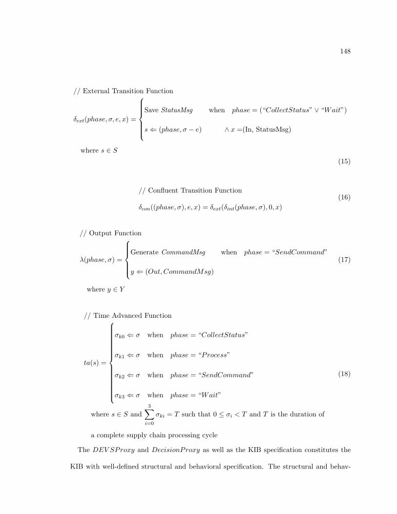
148
// External Transition Function
δext(phase, σ, e, x) =
Save StatusMsg when phase = (“CollectStatus” ∨ “Wait”)
s ⇐ (phase, σ − e) ∧ x =(In, StatusMsg)
where s ∈ S
(15)
// Confluent Transition Function
δcon((phase, σ), e, x) = δext(δint(phase, σ), 0, x)(16)
// Output Function
λ(phase, σ) =
Generate CommandMsg when phase = “SendCommand”
y ⇐ (Out,CommandMsg)
where y ∈ Y
(17)
// Time Advanced Function
ta(s) =
σk0 ⇐ σ when phase = “CollectStatus”
σk1 ⇐ σ when phase = “Process”
σk2 ⇐ σ when phase = “SendCommand”
σk3 ⇐ σ when phase = “Wait”
where s ∈ S and3∑
i=0
σki = T such that 0 ≤ σi < T and T is the duration of
a complete supply chain processing cycle
(18)
The DEV SProxy and DecisionProxy as well as the KIB specification constitutes the
KIB with well-defined structural and behavioral specification. The structural and behav-
149
ioral specification defines the message transformation, synchronization, and timing for the
disparate model interactions. The interaction specification by itself cannot guarantee the
correct execution among the disparate models unless a well-defined execution control is
defined to coordinate the execution among the disparate models.
7.3 Parallel Execution Control
In the KIBDEV S/MPC , we have designed and implemented the sequential execution control
scheme to process the interaction between DEVS and MPC. In the KIBDEV S/LP/MPC , a
parallel execution protocol is defined to support concurrent execution among the DEVS,
LP, MPC, and the KIB models.
As the bridges between the KIB and the disparate models, the sub-model DEVSProxy
and DecisionProxy can be executed in the disparate model execution context. For example,
the actual implementation of the Proxy interface needs to handle how to communicate
with the composing model which is implemented in a distinct modeling environment. The
KIBExecutor is defined to coordinate the executions among the proxy model executions
— i.e., executors for DEVS, LP, and MPC models.
As the KIB execution engine, KIBExecutor is desired to provide the following capabilities
for the constituent proxy models.
� Communication capability with each participating proxy model. Given the fact that
each disparate model is executed in its own context, certain communication capability
are needed between different executers. Queue and shared storage place can be used
for non-blocking communication.
150
� KIBTransformer. This is an engine that handles message transformations between
the disparate models given the KIB specification. The interaction messages between
the disparate models should be stored in order to support flexible KIB execution.
� Timing information
TCDEV S : unit processing time of the simulation model, such as one day or one hour.
TCD : unit decision time for each decision model. As we have addressed earlier,
the unit decision time is specified in the KIB specification. The interaction fre-
quency between the simulation model and the decision model or between the
disparate decision models is determined by the TCDEV S and TCD. For exam-
ple, FDEV S/MPC = TCMPC/TCDEV S , where the FDEV S/MPC is the interaction
frequency between DEVS and MPC. Similarly, the FMPC/LP = TCLP /TCMPC .
T and TN : discretized logical time used to keep current time and next time within
the KIB (T ∈ {0, N+}) and generally TN = T + TCDEV S . The computation
of the decision model (LP or MPC) is considered to be discretized in time.
Therefore, the timing information kept in the KIB is desired to be discretized.
The DEVS simulation time can be used to provide the discretized time, since the
DEVS is using continuous time and is capable of supporting discretized time. In
addition, it is convenient to use the simulation time to synchronize the composite
model execution.
� Parallel execution identification and control. Whether the disparate models can be
executed concurrently at runtime depends on not only the parallel execution scheme
but the composite model specification as well. That is, the data dependence implied
through the message transformation plays an important role in determining the ex-
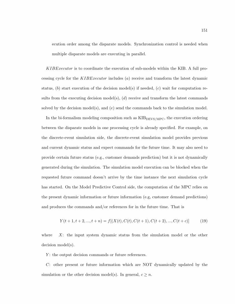
151
ecution order among the disparate models. Synchronization control is needed when
multiple disparate models are executing in parallel.
KIBExecutor is to coordinate the execution of sub-models within the KIB. A full pro-
cessing cycle for the KIBExecutor includes (a) receive and transform the latest dynamic
status, (b) start execution of the decision model(s) if needed, (c) wait for computation re-
sults from the executing decision model(s), (d) receive and transform the latest commands
solved by the decision model(s), and (e) send the commands back to the simulation model.
In the bi-formalism modeling composition such as KIBDEVS/MPC, the execution ordering
between the disparate models in one processing cycle is already specified. For example, on
the discrete-event simulation side, the discrete-event simulation model provides previous
and current dynamic status and expect commands for the future time. It may also need to
provide certain future status (e.g., customer demands prediction) but it is not dynamically
generated during the simulation. The simulation model execution can be blocked when the
requested future command doesn’t arrive by the time instance the next simulation cycle
has started. On the Model Predictive Control side, the computation of the MPC relies on
the present dynamic information or future information (e.g, customer demand predictions)
and produces the commands and/or references for in the future time. That is
Y (t + 1, t + 2, ..., t + n) = f [(X(t), C(t), C(t + 1), C(t + 2), ..., C(t + c)] (19)
where X: the input system dynamic status from the simulation model or the other
decision model(s).
Y : the output decision commands or future references.
C: other present or future information which are NOT dynamically updated by the
simulation or the other decision model(s). In general, c ≥ n.
152
Hence, the execution ordering between the disparate model is clear and no conflict can
happen. In comparison to the bi-formalism modeling composition, the execution order in
the multi-formalism modeling composition is more complex. At certain time instance, the
interaction between the process simulation model and the decision model is considered to
be the same as in the bi-formalism. But the interaction between two disparate decision
models is more intricate:
1. if both need only the past information from each other, they can run simultaneously,
2. if one needs present or future information, they must run in sequence, and
3. in case both need present or future information from the other model, the composite
model cannot be executed due to the conflict.
Therefore the execution ordering between two disparate decision models must be explicitly
identified. The attribute TStart and TEnd in the element Transform is used to identify
the execution ordering of the disparate models. For a KIB message, its dynamic status is
updated by the Source model and the status is needed by the Destination model. On the
Source element side, the attribute TStart and TEnd of the Transform indicate that the
source model provides the dynamic status for the time [T + TStart, T + TEnd] (TStart ≤
TEnd) where T is the current time instance at which the message transformation is to
occur. On the Destination element side, the attributes TStart and TEnd imply that the
destination model needs the dynamic status at the time [T +TStart, T +TEnd] (TStart ≤
TEnd). Given the fact that for a discrete-time model, timing must be advanced after each
computation, it is required that (TEnd ≥ TStart > 0) except at the initialization, if the
Source model is a decision model.
153
For two disparate decision models that have interactions, the execution ordering between
the two decision models can be computed as follows
When (Source.TStart > Destination.TEnd) Concurrency is allowed, since the status is
already available for Destination model at the time of interaction.
When (Source.TStart ≤ Destination.TEnd) The Source model must be executed before
Destination, since the Destination model relies on the status which is being computed
by the Source model at the time of interaction.
When (Source.TEnd < Destinaton.TEnd) The composite model is invalid, since the Des-
tination model relies on the status which cannot be provided by the Source model at
the time of interaction.
The execution ordering algorithm needs to be applied for all the KIB messages in the
specification to identify the execution ordering of all the participating disparate decision
models. Therefore, we can also detect whether there exist any potential deadlocks between
any two disparate decision models—when the execution ordering between two disparate
decision conflicts in different message transformations. With the KIB specification, we can
not only identify the execution ordering among the disparate models but also verify the
composite model. The execution ordering should be identified at the initialization stage to
ensure no deadlock would occur during the KIB executor.
Given the considerations addressed above, an execution protocol for the KIBExecutor
is defined to control the KIBDEVS/LP/MPC execution and coordinate the executions among
DEVS, LP, and MPC thereafter. It is assumed that there are 2 disparate decision models
(i.e., one LP model and one MPC model) participating in the supply-chain management

154
against the process model. And the DEV Proxy is initialized when the process simulation
model is initialized.
� Initialization
1. T = 0, TN = TCDEV S
2. instantiate the decision model DProxyLP and DProxyMPC
3. QDEV S = NULL
4. set execution ordering for the decision model OrderLP and OrderMPC
– if (isInvalid(ordering)) then EXIT
� Loop: when T 6= ∞
1. Wait until StatusMsg arrives at QDEV S
2. Process simulation messages. For each message m in QDEV S
– if (m is StatusMsg) then KIBTransformer → UpdateStatus(m,T )
– if (m is TimeMsg) then TN := m.V alue
– Reset QDEV S
3. Start Decision models. For DProxyLP and DProxyMPC
– if (TN mod TCDLP== 0) then
DProxyLP → Execute(T )
– if (TN mod TCDMPC== 0) then
DProxyMPC → Execute(T )
4. Process Decision messages. For DProxyLP and DProxyMPC
155
– if (OrderLP ≤ OrderMPC) then
wait until DProxyLP → GetState() == IDLE
wait until DProxyMPC → GetState() == IDLE
– if (OrderLP > OrderMPC) then
wait until DProxyMPC → GetState() == IDLE
wait until DProxyLP → GetState() == IDLE
5. Update Time: T = TN
6. Generate simulation command messages.
– mc := KIBTransformer → GetCommand(T )
– send mc to QDEV S
� Termination: when TN = ∞
The computations of the decision models (LP and MPC) are assumed to occur at dis-
cretized time instances in order to get synchronized. Their execution must be synchronized
at discrete time. In the execution control described above, the simulation time in the DEVS
is utilized as the global logical simulation time across the composite DEVS/LP/MPC model.
The simulation time is kept as continuous on the simulation side. It is discretized when
the time message (TimeMessage) is sent to the KIBExecutor. Therefore, the value car-
ried by the TimeMessage is T ∈ (0 ∪ N+) (see Figure 33). At a certain time instance,
all the decision models are scheduled to be executed in some predefined order. With the
timing synchronization, the decision models that are in the same ordering can be executed
simultaneously. It is required to wait for all the executing decision models to complete
before starting the decision models in the next scheduling order. The time kept in the KIB
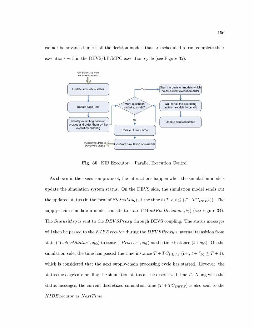
156
cannot be advanced unless all the decision models that are scheduled to run complete their
executions within the DEVS/LP/MPC execution cycle (see Figure 35).
Fig. 35. KIB Executor— Parallel Execution Control
As shown in the execution protocol, the interactions happen when the simulation models
update the simulation system status. On the DEVS side, the simulation model sends out
the updated status (in the form of StatusMsg) at the time t (T < t ≤ (T +TCDEV S)). The
supply-chain simulation model transits to state (“WaitForDecision”, δ0) (see Figure 34).
The StatusMsg is sent to the DEV SProxy through DEVS coupling. The status messages
will then be passed to the KIBExecutor during the DEV SProxy’s internal transition from
state (“CollectStatus”, δk0) to state (“Process”, δk1) at the time instance (t+ δk0). On the
simulation side, the time has passed the time instance T + TCDEV S (i.e., t + δk0 ≥ T + 1),
which is considered that the next supply-chain processing cycle has started. However, the
status messages are holding the simulation status at the discretized time T . Along with the
status messages, the current discretized simulation time (T + TCDEV S) is also sent to the
KIBExecutor as NextT ime.
157
At the time instance when KIBExecutor processes the DEVS messages, the discretized
time inside KIB is kept as time T , which is set in the precious KIB processing cycle.
The simulation status at time T is then stored within KIB. Then KIBExecutor needs
to determine which decision models should be executed at time T . Due to the different
unit decision time instances, one or more decision models may need to be executed. If
both LP and MPC decision model need to be executed, they are triggered simultaneously
by the KIBExecutor. The decision models start their computation in their own contexts
(i.e., each DecisionProxy provides an independent execution context for the associated
decision model). Whether the corresponding decision model can actually start computation
is determined by whether the input variable values required at the time T is ready or not.
If the input variable values is not ready, the DecisionProxy will block its computation.
Since the data dependency between the decision models has been identified, at least one
decision model can start the execution. Thereafter, the decision model(s) that are blocked
are unblocked and start their executions. Given the synchronization control on the decision
model executions, the time in KIB cannot be advanced before all the executing decision
models finish the computation1 The waiting ordering should be consistent with the execution
ordering: wait for the decision model which has the first execution order first.
Computation results from the decision models thereafter can be used to generate de-
cision commands for the simulation model at time T + TCDEV S . The time in KIB is
then advanced to T + TCDEV S . The decision command messages (CommandMsg) are
sent back to DEV SProxy via messaging passing. For the DEV SProxy, the command
messages are fetched during the internal transition from the state (“Process”, δk1 to the
state (“SendCommand”, δk2), at which the time has been advanced to (t + δk0 + δk1).
1The blocking issues due to hardware failure (e.g., networking and computer problems)is not considered in the scope of this work.
158
The simulation executor cannot continue its execution until the DEV SProxy receives the
command messages. This blocking is needed, since the simulation model needs the com-
mand messages to continue its execution. When the command messages are available, the
DEV SProxy can continue its state transition from the state (“Process”, δk1) to the state
(“SendCommand”, δk3). Before its state is changed to (“Wait”, δk3), DEV SProxy sends
the command messages to the process simulation models through DEVS couplings. The sim-
ulation time becomes (t+δk0+δk1+δk2) at this time instance. Given the specification of the
Sigma (δ0) for the phase (“waitingForDecision”) in the supply-chain manufacturing mod-
els, (δ0 > δk0 + δk1 + δk2). Therefore, the command messages can arrive at the supply-chain
simulation model before the simulation model changes the state to (“StartMaterial”, δ1)
(see Figure 19). The combination of DEVS simulation protocol and KIBExecutor parallel
execution control ensures the causal ordering of the messages produced & consumed during
the interactions among the disparate models.
Given the KIB specification, deadlock detection can be carried out during the composite
model initialization. It is beneficial for verifying composite model and simplifying the
parallel execution control.
7.4 Software Design of Hybrid DEVS/LP/MPC Distributed Simulation Frame-
work
A prototypical distributed simulation framework was designed and developed to support
composing DEVS, LP, and MPC models. This framework is built on the basis of the
KIBDEVS/LP/MPC specification and its parallel execution protocol specified in the previous
section. It supports distributed execution of the disparate models with parallel execution
control.
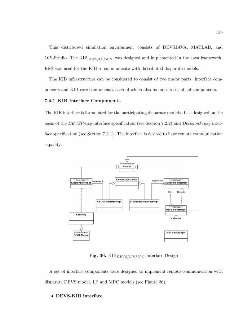
159
This distributed simulation environment consists of DEVSJAVA, MATLAB, and
OPLStudio. The KIBDEVS/LP/MPC was designed and implemented in the Java framework.
RMI was used for the KIB to communicate with distributed disparate models.
The KIB infrastructure can be considered to consist of two major parts: interface com-
ponents and KIB core components, each of which also includes a set of subcomponents.
7.4.1 KIB Interface Compoments
The KIB interface is formulated for the participating disparate models. It is designed on the
basis of the DEVSProxy interface specification (see Section 7.2.2) and DecisionProxy inter-
face specification (see Section 7.2.1). The interface is desired to have remote communication
capacity.
Fig. 36. KIBDEV S/LP/MPC Interface Design
A set of interface components were designed to implement remote communication with
disparate DEVS model, LP and MPC models (see Figure 36).
� DEVS-KIB interface
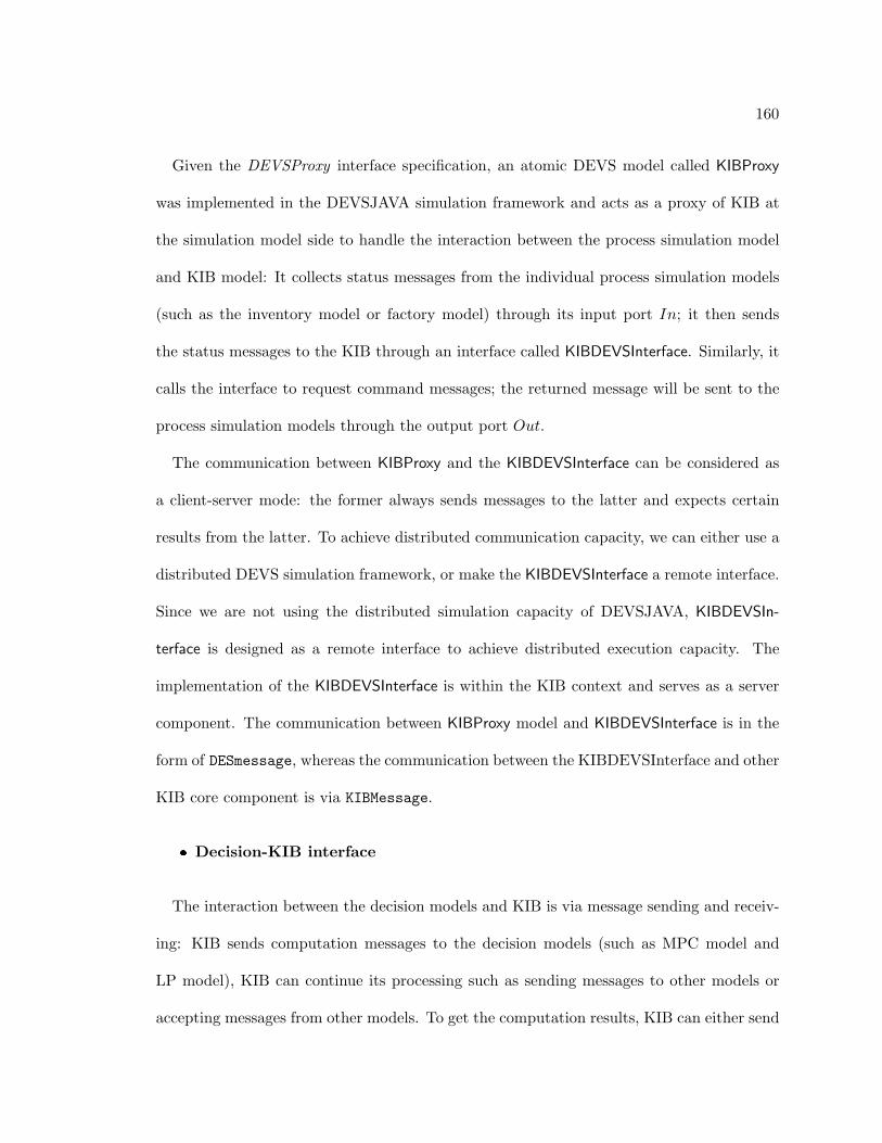
160
Given the DEVSProxy interface specification, an atomic DEVS model called KIBProxy
was implemented in the DEVSJAVA simulation framework and acts as a proxy of KIB at
the simulation model side to handle the interaction between the process simulation model
and KIB model: It collects status messages from the individual process simulation models
(such as the inventory model or factory model) through its input port In; it then sends
the status messages to the KIB through an interface called KIBDEVSInterface. Similarly, it
calls the interface to request command messages; the returned message will be sent to the
process simulation models through the output port Out.
The communication between KIBProxy and the KIBDEVSInterface can be considered as
a client-server mode: the former always sends messages to the latter and expects certain
results from the latter. To achieve distributed communication capacity, we can either use a
distributed DEVS simulation framework, or make the KIBDEVSInterface a remote interface.
Since we are not using the distributed simulation capacity of DEVSJAVA, KIBDEVSIn-
terface is designed as a remote interface to achieve distributed execution capacity. The
implementation of the KIBDEVSInterface is within the KIB context and serves as a server
component. The communication between KIBProxy model and KIBDEVSInterface is in the
form of DESmessage, whereas the communication between the KIBDEVSInterface and other
KIB core component is via KIBMessage.
� Decision-KIB interface
The interaction between the decision models and KIB is via message sending and receiv-
ing: KIB sends computation messages to the decision models (such as MPC model and
LP model), KIB can continue its processing such as sending messages to other models or
accepting messages from other models. To get the computation results, KIB can either send
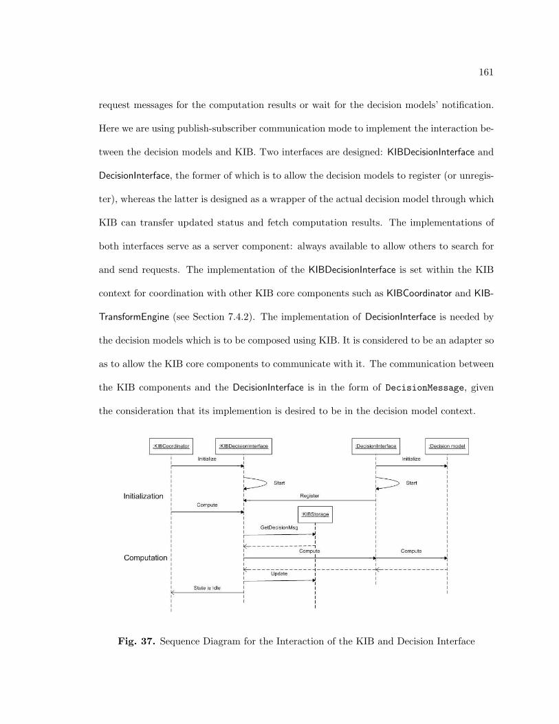
161
request messages for the computation results or wait for the decision models’ notification.
Here we are using publish-subscriber communication mode to implement the interaction be-
tween the decision models and KIB. Two interfaces are designed: KIBDecisionInterface and
DecisionInterface, the former of which is to allow the decision models to register (or unregis-
ter), whereas the latter is designed as a wrapper of the actual decision model through which
KIB can transfer updated status and fetch computation results. The implementations of
both interfaces serve as a server component: always available to allow others to search for
and send requests. The implementation of the KIBDecisionInterface is set within the KIB
context for coordination with other KIB core components such as KIBCoordinator and KIB-
TransformEngine (see Section 7.4.2). The implementation of DecisionInterface is needed by
the decision models which is to be composed using KIB. It is considered to be an adapter so
as to allow the KIB core components to communicate with it. The communication between
the KIB components and the DecisionInterface is in the form of DecisionMessage, given
the consideration that its implemention is desired to be in the decision model context.
Fig. 37. Sequence Diagram for the Interaction of the KIB and Decision Interface
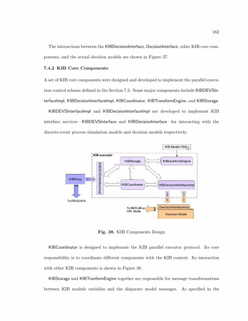
162
The interactions between the KIBDecisionInterface, DecisionInterface, other KIB core com-
ponents, and the actual decision models are shown in Figure 37.
7.4.2 KIB Core Components
A set of KIB core components were designed and developed to implement the parallel execu-
tion control scheme defined in the Section 7.3. Some major components include KIBDEVSIn-
terfaceImpl, KIBDecisionInterfaceImpl, KIBCoordinator, KIBTransformEngine, and KIBStorage.
KIBDEVSInterfaceImpl and KIBDecisionInterfaceImpl are developed to implement KIB
interface services—KIBDEVSInterface and KIBDecisionInterface—for interacting with the
discrete-event process simulation models and decision models respectively.
Fig. 38. KIB Components Design
KIBCoordinator is designed to implement the KIB parallel executor protocol. Its core
responsibility is to coordinate different components with the KIB context. Its interaction
with other KIB components is shown in Figure 38.
KIBStorage and KIBTranformEngine together are responsible for message transformations
between KIB module variables and the disparate model messages. As specified in the
163
Section 7.1.4, each message in one disparate model which has interactions with the other
disparate models has a corresponding module message in the KIB specification. KIBStorage
is the KIB storage space where a set of KIB modules are held, each of which consists of a
set of KIB variables. For each KIB variable, it is composed of one source model reference
and one or more destination model references as well as their transformation configuration.
The KIB variables are time stamped using discrete-time. KIBTransformEngine interprets
the transformation configuration specified in the KIB specification and implement data
transformations between KIB variables and disparate model messages.
The supply-chain network system described in Figure 30 has been modeled in the dis-
tributed simulation framework. The process simulation models developed in Section 6.1.1
were used as the network processing models, the MATLAB engine implemented in the
KIBDEVS/MPC framework was extended to implement interaction with the actual MPC
model within the DecisionInterfaceImpl—an implementation of the interface DecisionInter-
face. The OPL Studio engine implemented in the [27] can be extended to support interaction
with the actual LP model developed in OPLStudio modeling environment. These model
components were deployed in multiple computers (shown in Figure 39) and they interact
with each other via RMI technology.
7.5 Summary
An extended KIB message transformation specification with a parallel execution control
scheme was proposed in this chapter. This KIB supports composing discrete-even simula-
tion model with both MPC model and LP model. The design of a prototypical distributed
simulation framework using KIBDEVS/LP/MPC approach was described thereafter. The hy-
brid simulation framework can support distributed simulation of a semiconductor manufac-
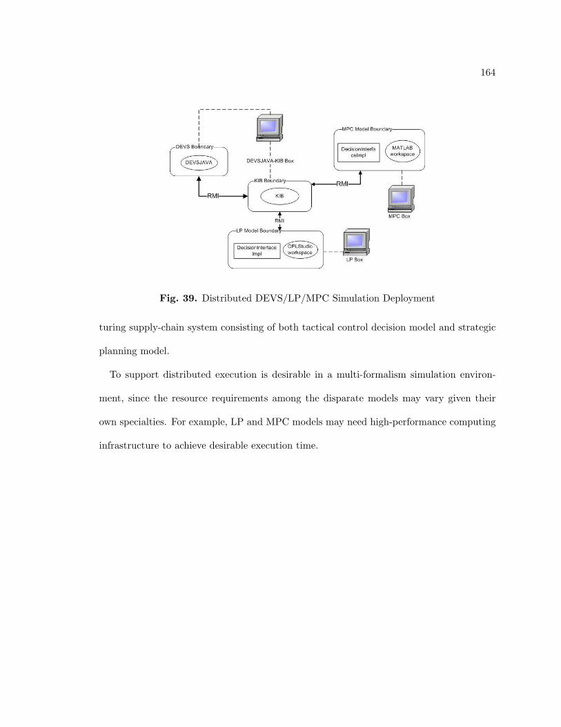
164
Fig. 39. Distributed DEVS/LP/MPC Simulation Deployment
turing supply-chain system consisting of both tactical control decision model and strategic
planning model.
To support distributed execution is desirable in a multi-formalism simulation environ-
ment, since the resource requirements among the disparate models may vary given their
own specialties. For example, LP and MPC models may need high-performance computing
infrastructure to achieve desirable execution time.
CHAPTER 8
CONCLUSION AND FUTURE WORK
In this dissertation, a novel modeling composition approach — Knowledge Interchange
Broker (KIB) was proposed to achieve composability across multiple modeling formalisms
where complex data transformations and synchronized execution between disparate models
can be described. As demonstrated in the previous chapters, the KIB approach exhibited
its flexibility and scalability in composing discrete-event simulation, linear programming,
and model predictive control models in a systematic manner. The KIB approach provided
a basis at the modeling level for the construction of hybrid simulation environments to
observe, analyze, and resolve complex problems occurring in the supply chain systems such
as semiconductor manufacturing supply-chain systems.
8.1 Conclusions
The conceptual basis of the KIB approach is to support model composability. The fun-
damental purpose of the KIB is to characterize the interactions among disparate models
at the level of modeling formalisms. With this multi-formalism modeling composition ap-
proach, the characteristics of model heterogeneity is carried out with KIB specification and
its corresponding executor. Together, they account for the modeling formalism specialties
in syntax and semantics and thus provide generalized support for data and control inter-
action. The KIB composition is an independent model specification between the disparate
models to explicitly describe the interaction activities in term of message transformation,
concurrency, synchronization, and timing properties.
Using the KIB approach, a novel interaction model — KIBDEVS/MPC was created to sup-
port composing complementary DEVS process simulation and MPC tactical models. The
KIB specification accounted for the differences on the interface messages — i.e., how to
transform DEVS messages (〈Model, Port, Message〉) to MPC numeric variables (〈Model,
166
vector, index〉), and vise versa. DEVS timing property and DEVS simulation protocol were
utilized to achieve time synchronization and concurrency between the DEVS simulation
model and the KIB model, since DEVS provides a well-defined simulation protocol to sup-
port timing and message causality. A restricted synchronization control is provided in the
KIB executor to support sequential execution among the disparate models and the KIB
model.
An experimental testbed was then designed and implemented using the KIBDEVS/MPC
specification. The testbed using the hybrid DEVSJAVA/MATLAB environment supported
flexibility for observing and analyzing how discrete-event processes and control policies af-
fect each other. This testbed was applied to a prototypical semiconductor manufacturing
supply-chain system. It provided the capabilities of independent evaluation of the manufac-
turing processes, tactical control scheme, and their interactions. The experiments revealed
the impact of realistic non-linearity and stochasticity of the manufacturing dynamics and its
importance in designing suitable tuning control parameters. The simulated responses show
the ability of the MPC controller to maintain stable, robust operation under conditions of
nonlinearity and uncertainty in the manufacturing plant dynamics. The simulation studies
helped uncover and explain complex relationships between control policies and manufactur-
ing processes.
The KIBDEVS/MPC was then extended to create a new KIBDEVS/LP/MPC for the compo-
sition of multiple DEVS, LP, and MPC modeling formalisms. A causal parallel execution
protocol was devised to allow for concurrent executions among the disparate models and
the KIB model. In this parallel execution scheme, logical time was used to synchronize the
executions between the DEVS simulation model and the KIB model. The synchronization
between the KIB model and the decision model(s) was treated as discrete-time execution.
167
Although the parallel execution scheme supports concurrency among the disparate model
executions, how the disparate models were executed at runtime relied on appropriate tim-
ing&message dependency specifications of the system. The parallel execution protocol was
particularly beneficial if the discrete process simulation model is controlled by multiple
independent decision models.
Given the KIBDEVS/LP/MPC and the proposed parallel execution protocol, the
DEVS/MPC bi-formalism modeling composition framework was extended to support the
composition of DEVS, LP, and MPC models. The parallel execution protocol as well the
distributed simulation was designed and implemented in the framework to demonstrate the
correctness of the multi-formalism composition with parallel execution control. The KIB
specification and its execution protocol is intended to be independent of software realization.
For example, JAVA RMI was used to communicate the distributed components developed
in DEVSJAVA, MATLAB, and OPL Studio. This technology can be replaced by other
middleware techniques such as CORBA.
The modeling composition framework using KIB approach is application neutral. It
can be adapted to model and simulate other network systems where the dynamics of the
process subsystem is periodically controlled by some other decision subsystem(s). Prior to
this work, no other poly-formalism modeling composability framework has been reported
for discrete-event and predictive control models. These capabilities support a new kind
of modeling and simulation verification and validation through explicit representation and
execution of model interactions in a systematic way.
In conclusion, a set of key benefits of using the KIB approach for model composition have
been presented in this dissertation. The poly-formalism composability approach
168
� exhibits the flexibility and scalability to support composing discrete-event simulation
modeling, linear programming, and model predictive control modeling in a systematic
way,
� supports independent evaluation of disparate models as well as their interactions,
� offers a generalized basis toward model validation and verification for heterogeneous
systems, and
� provides a layer of general-purpose multi-formalism modeling composition which can
be applied to different application domains.
8.2 Future Work
Currently XML is used to specify KIB message transformation and time synchronization.
The specification has to be done manually. It is desired to provide a mechanism to enable
automatic message transformation for a given application domain such as semiconductor
supply chain systems. Furthermore, the automation may help validate and verify the cor-
rectness of the composite model. For example, in the process of specifying the message
transformation, a set of rules can be constructed to detect any conflicts such as the incon-
sistencies and the paradox in the data dependency & timing among disparate models.
In the current KIB composition, three modeling formalisms — i.e., DEVS, LP and
MPC—are desired to be composed. Both LP and MPC can be considered to execute as
discrete-time models, therefore they can be treated as one family of modeling formalisms.
An ongoing research is applying the KIB theory for composing rule-based discrete-event
and cellular automata models ([50, 49]). Although KIB provides a conceptual basis of poly-
formalism modeling composition, to identify the structural and behavioral distinction and
handle their interactions among the other kinds of modeling formalisms remains as future

169
research. In addition, the KIB specification may need to be further studied when applying
the KIB approach to other problem domains such as the socio-ecological domain.
Service-oriented architecture technologies are being used for simulation interoperability
and primarily syntactical composition of un-timed models. How to map the KIB speci-
fication to a set of service specification and thus supporting service-oriented KIB model
composition and execution is another future research area.
REFERENCES
[1] ACIMS. DEVSJAVA, 2004. Available from http://acims.eas.asu.edu/SOFTWARE/software.shtml.
[2] T. Andrews, F. Curbera, H. Dholakia, Y. Goland, and J. Klein. Business ProcessExecution Language for Web Services (v1.1), 2003. Available from http://download.boulder.ibm.com/ibmdl/pub/software/dw/specs/ws-bpel/ws-bpel.pdf.
[3] B. J. Angerhofer and M. C. Angelides. System dynamics modelling in supply chainmanagement: Research review. In Proceedings of Winter Simulation Conference,pages 342–351, San Diego, CA, USA, 2000.
[4] F. Arbab. Abstract behavior types: a foundation model for components and theircomposition. Science of Computer Programming, 55(1-3):3–52, 2005.
[5] M. W. Braun, D. E. Rivera, M. E. Flores, W. M. Carlyle, and K. G. Kempf. Amodel predictive control framework for robust management of multi-product multi-echelon demand networks. Special Issues on Enterprise Integration and Networking,27:229–245, 2003.
[6] F. Buschmann, R. Meunier, H. Rohnert, P. Sommerlad, and M. Stal. Pattern-OrientedSoftware Architecture: a System of Patterns. John Wiley & Sons, Inc, 1996.
[7] Y. Cho, B. Zeigler, and H. Sarjoughian. Design and implementation of distributedreal-time DEVS/CORBA. In IEEE Sys. Man. Cyber Conference, pages 3081–3086,Tucson, AZ, USA, 2001.
[8] R. Christie and S. Wu. Semiconductor capacity planning: Stochastic modeling andcomputational studies. IIE Transactions on Design & Manufacturing, 24(2):131–143,2002.
[9] DashOptimization. XPRESS-MP, 2005. Available from http://www.dashoptimization.com/.
[10] P. Davis and R. Anderson. Improving the Composability of Department of DefenseModels and Simulations. RAND, Santa Monica, CA, USA, 2004.
[11] P. C. Davis, C. M. Overstreet, P. A. Fishwick, and C. D. Pegden. Model composabilityas a research investment: Responses to the featured paper. In Proceedings of WinterSimulation Conference, 2000.
[12] J. de Lara, H. Vangheluwe, and M. Alfonseca. Meta-modelling and graph grammarsfor multi-paradigm modelling in atom3. Software and System Modelling, 3(3):194–209,2004.
171
[13] J. Eker, J. Janneck, E. Lee, J. Liu, X. Liu, J. Ludvig, S. Neuendorffer, S. Sachs, andY. Xiong. Taming heterogeneity—the ptolemy approach. Proceedings of the IEEE,2(91):127–144, 2003.
[14] T. Eldabi, J. Ray, and R. Paul. Flexible modeling of manufacturing systems withvariable levels of details. In Proceedings of Winter Simulation Conference, Atlanda,GA, USA, 1997.
[15] R. J. Firby and W. Fitzgerald. The RAP System Language Manual, Version 2.0.Neodesic Corporation, Evanston, IL, USA, 1999.
[16] J. W. Forrester. Industrial Dynamics. MIT Process, Cambridge, MA, USA, 1961.
[17] I. Foster, C. Kesselman, and S. Tuecke. The anatomy of the grid: Enabling scal-able virtual organizations. International Journal of High Performance ComputingApplications, 3(15):200–222, 2001.
[18] I. Foster, H. Kishimoto, A. Savva, D. Berry, A. Djaoui, A. Grimshaw, and B. Horn.The Open Grid Service Architectures, Version 1.0, 2005. Available from http://www.gridforum.org/documents/GWD-I-E/GFD-I.030.pdf.
[19] J. W. Fowler and O. Rose. Grand challenges in modeling and simulation of complexmanufacturing systems. Simulation, 80(9):469–476, 2004.
[20] R. Fujimoto. Parallel and Distributed Simulation Systems. John Wiley and Sons Inc.,2000.
[21] R. Fujimoto. Parallel and distributed simulation systems. In Proceedings of WinterSimulation Conference, pages 147–157, Arlington, VA, USA, 2001.
[22] R. Garcia-Flores and X. Wang. A multi-agent system for chemical supply chainsimulation and management support. OR Spectrum, 24:343–370, 2002.
[23] J. Gjerdrum, N. Shah, and L. G. Papageorgiou. A combined optimization and agent-based approach to supply chain modelling and performance assessment. ProductionPlanning & Control, 12(1):81–88, 2001.
[24] Globus. Globus ToolKit, 2005. Available from http://www.globus.org/toolkit/.
[25] G. Godding. Discrete Event and Optimization Multi-Modeling Methodology for Sim-ulating Semiconductor Supply-Chain Systems. PhD thesis, Computer Science and
172
Engineering Department, School of Computing and Informatics, Arizona State Uni-versity, Tempe, AZ, USA, 2008.
[26] G. Godding, H. Sarjoughian, and K. Kempf. Semiconductor supply network simula-tion. In Proceedings of Winter Simulation Conference, pages 1593–1601, WashingtonDC, USA, 2003.
[27] G. Godding, H. Sarjoughian, and K. Kempf. Multi-formalism modeling approachfor semiconductor supply/demand networks. In Proceedings of Winter SimulationConference, pages 232–239, Washington DC, USA, 2004.
[28] G. Godding, H. Sarjoughian, and K. Kempf. Application of combined discrete-eventsimulation and optimization models in semiconductor enterprise manufacturing sys-tems. In Proceedings of Winter Simulation Conference, pages 232–239, WashingtonDC, USA, 2007.
[29] HLA. IEEE Standard for Modeling and Simulation (M&S) High Level Architecture(HLA)—Federate Interface Specification. IEEE, 2000.
[30] M. Hocaoglu, H. Sarjoughian, and C. Firat. DEVS/RAP: Agent-based simulation.In AI, Simulation and Planning in High-Autonomy Systems, Lisbon, Portual, 2002.SCS.
[31] A. T. Hofkamp and J. E. Rooda. Chi Reference Manual, 2008. Available from http://w3.wtb.tue.nl/nl/organisatie/systems_engineering/se_documentation/.
[32] D. Huang, H. Sarjoughian, W. Wang, G. Godding, D. Rivera, K. Kempf, and H. Mit-telmann. Simulation of semiconductor manufacturing supply-chain systems withDEVS, MPC, and KIB. the Special Issues of IEEE Transactions on Semiconduc-tor Manufacturing, accepted under revision, 2007.
[33] D. Huang, H. S. Sarjoughian, D. E. Rivera, G. W. Godding, and K. G. Kempf. Flexibleexperimentation and analysis for hybrid DEVS and MPC models. In Proceedings ofWinter Simulation Conference, Monterey, CA USA, 2006.
[34] Y.-F. Hung and R. C. Leachman. A production planning methodology for semiconduc-tor manufacturing based on iterative simulation and linear programming calcuations.IEEE Transactions on Semiconductor Manufacturing, 9(2):257–269, 1996.
[35] i2. http: // www. supply-chain. org , 2006.
173
[36] ILOG. OPL Studio, 2005. Available from http://www.ilog.com/products/oplstudio/.
[37] S. Jain, C.-C. Lim, B.-P. Gan, and Y.-H. Low. Criticality of detailed modeling in semi-conductor supply chain simulation. In Proceedings of Winter Simulation Conference,1999.
[38] K. Kempf. Control-oriented approaches to supply chain management in semiconductormanufacturing. In Proceedings of IEEE American Control Conference, pages 4563–4576, Boston, MA, USA, 2004.
[39] J. P. Kleijnen. Supply chain simulation: a survey. International Journal of Simulationand Process Modeling, 2003.
[40] J. P. C. Kleijnen and M. T. Smith. Performance metrics in supply chain management.Journal of Operational Research Society, 54:507–514, 2003.
[41] E. Kofman. Discrete-event simulation of hybrid systems. SIAM Journal of ScientificComputing, 25(5):1771–1797, 2004.
[42] E. A. Lee and Y. Xiong. Behavioral types for component-based design. Departmentof Electrical Engineering and Computer Sciences, University of California, Berkley,CA, 2002.
[43] P. Lendermann, N. Julka, B. P. Gan, D. Chen, L. F. McGinnis, and J. P. McGinnis.Distributed supply chain simulation as a decision support tool for the semiconductorindustry. Simulation, 79(3):126–138, 2003.
[44] F. Leymann. Web Services Flow Language (WSFL 1.0), 2001. Available from http://www-306.ibm.com/software/solutions/webservices/pdf/WSFL.pdf.
[45] J. Liu, J. Eker, J. Janneck, X. Liu, and E. Lee. Actor-oriented control system design:a reasonal framework perspective. IEEE Transactions on Control Systems Technology,12(2):250–262, 2004.
[46] R. R. Lummus and R. J. Vokurka. Defining supply chain management: a historicalperspective and practical guidelines. Industrial Management & Data Systems, 1:11–17, 1999.
[47] Mathworks. MATLAB Optimization Toolbox, 2005. Available from http://www.mathworks.com/products/optimization/.
174
[48] Mathworks. MATLAB/Simulink, 2005. Available from http://www.mathworks.com.
[49] G. Mayer and H. Sarjoughian. Complexities of simulating a hybrid agent-landscapemodel using multi-formalism composability. In Agent-Directed Simulation, SpringSimulation Multiconference, pages 161–168, Norfolk, Virginia, USA, 2007.
[50] G. Mayer, H. Sarjoughian, E. Allen, S. Falconer, and M. Barton. Simulation modelingfor human community and agricultural landuse. In Agent-Directed Simulation, SpringSimulation Multiconference, pages 65–72, Huntsville, AL, USA, 2006.
[51] MDA. Model Driven Architecture, 2008. Available from http://www.omg.org/mda.
[52] N. Mehta, N. Medvidovic, M. Sirjani, and F. Arbab. Modeling behavior in compo-sitions of software architectural primitives. In Proceedings of the 19th InternationalConference on Automated Software Engineering, pages 371–374. IEEE Computer So-ciety, 2004.
[53] Microsoft. DCOM Architecture, 2008. Available from http://msdn2.microsoft.com/en-us/library/ms809311.aspx.
[54] Microsoft. .Net Framework 3.5, 2008. Available from http://msdn2.microsoft.com/en-us/library/w0x726c2.aspx.
[55] Microsoft. Windows Communication Foundation, 2008. Available from http://msdn2.microsoft.com/en-us/library/ms735119.aspx.
[56] S. Microsystems. JAVA RMI Specification, 2008. Available from http://java.sun.com/javase/6/docs/platform/rmi/spec/rmiTOC.html.
[57] H. Min and G. Zhou. Supply chain modeling: Past, present and future. Computers& Industrial Engineering, 43:231–249, 2002.
[58] L. Monch, O. Rose, and R. Sturm. A simulation framework for the performanceassessment of shop-floor control systems. Simulation, 79(3):163–170, 2003.
[59] P. Mosterman and H. Vangheluwe. Guest editorial: Special issues on computer au-tomated multi-paradigm modeling. ACM Transaction on Modeling and ComputerSimulation, 4(12):249–255, 2002.
[60] P. Mosterman and H. Vangheluwe. Computer automated multi-paradigm modeling:An introduction. Transaction of the Society for Modeling and Simulation Interna-tional, 1(80):433–450, 2004.
175
[61] S. Muller. JMatLink, 2002. Available from http://www.held-mueller.de/JMatLink/.
[62] NRC. Modeling and Simulation in Manufacturing and Defense Acquisition: Path toSuccess. National Academy Press, Washington D.C., 2002.
[63] OMG. CORBA Specification, 2008. Available from http://www.omg.org/spec/CORBA/3.1/.
[64] Oracle. Oracle Supply Chain Management Solution, 2006. Available from http://www.oracle.com/applications/scm/index.html.
[65] M. Petty and E. W. Weisel. A composability lexicon. In Simulation InteoperabilityWorkshop, Orlando, FL, USA, 2003.
[66] H. Praehofer. System Theoretic Foundations for Combined Discrete Continuous Sys-tem Simulation. PhD thesis, Institute of Systems Science, Department of SystemsTheory and Information Engineering, Johannes Kelper University, 1991.
[67] Ptolemy. Ptolemy Project, 2008. Available from http://ptolemy.eecs.berkeley.edu/.
[68] S. J. Qin and T. A. Badgwell. A survey of industrial model predictive control tech-nology. Control Engineering Practice, 11(7):733–764, 2003.
[69] S. Ramakrishnan, S. Lee, and R. Wysk. Implementation of a simulation-based con-trol architecture for supply chain interactions. In Proceedings of Winter SimulationConference, pages 1667–1674, San Diego, CA, USA, 2002.
[70] S. Reveliotis. An Introduction to Linear Programming and the Simplex Algorithm,1997. Available from http://www2.isye.gatech.edu/~spyros/LP.
[71] C. E. Riddalls, S. Nennett, and N. S. Tipi. Modelling the dynamics of supply chains.International Journal of Systems Science, 31(8):969–976, 2001.
[72] D. Rivera, H. Sarjoughian, and K. Kempf. Control-oriented strategies for supply chainmanagement in semiconductor manuafacturing (proposal). Arizona State University,Tempe, AZ, 2004.
[73] Rockwell. Arena Simulation, 2008. Available from http://www.arenasimulation.com/.
176
[74] N. M. Sadeh, D. W. Hildum, D. Kjenstad, and A. Tseng. MASCOT: An agent-basedarchitecture for coordinated mixed-initiative supply chain planning and scheduling.In 3rd international Conference on Autonomous Agents Workshop on Agent-BasedDecision Support for Managing the Internet-Enabled Supply Chain, Seattle, WA, USA,1999.
[75] SAP. mySAP SCM, 2006. Available from http://www.sap.com/solutions/business-suite/scm.
[76] H. Sarjoughian and F. Cellier, editors. Discrete Event Modeling and Simulation Tech-nologies: A Tapestry of Systems and AI-Based Theories and Methodologies. SpringerVerlag., 2001.
[77] H. Sarjoughian and D. Huang. A multi-formalism modeling composition framework:Agent and discrete-event models. In Proceedings of the 9th IEEE International Sym-poisum on Distributed Simulation and Real Time Applications, pages 249–256, Mon-treal, Canada, 2005.
[78] H. Sarjoughian, D. Huang, W. Wang, D. E. Rivera, K. G. Kempf, G. W. Godding,and H. D. Mittelmann. Hybrid discrete event simulation with model predictive controlfor semiconductor supply-chain manufacturing. In Proceedings of Winter SimulationConference, pages 256–266, Orlando, FL, USA, 2005.
[79] H. Sarjoughian and J. Plummer. Design and Implementation of a Bridge betweenRAP and DEVS. Computer Science and Engineering, Arizona State University,Tempe, AZ, 2002. Internal report.
[80] H. Sarjoughian and B. Zeigler. DEVS and HLA: Complementary paradigms formodeling and simulation? Transaction of the Society for Modeling and SimulationInternational, 4(17):187–197, 2000.
[81] H. S. Sarjoughian. Model composability. In Proceedings of the Winter SimulationConference, pages 149–158, Montery, CA, USA, 2006.
[82] SCC. Supply-Chain Operations Reference Model (SCOR), 2005. Available from http://www.supply-chain.org.
[83] A. F. Seila. Spreadsheet simulation. In Proceedings of Winter Simulation Conference,pages 41–48, Washington D. C., USA, 2004.
[84] R. K. Singh, H. S. Sarjoughian, and G. W. Godding. Design of scalable simulationmodels for semiconductor manufacturing processes. In Proceedings of the SummerComputer Simulation Conference, pages 235–240, San Jose, CA, USA, 2004.
177
[85] J. M. Swaminathan. Modeling supply chain dynamics: a multiagent approach. Deci-sion Sciences, 29(3):607–632, 1998.
[86] S. Taylor, G. Popescu, J. Pullen, and S. Turner. Distributed simulation and thegrid: Position statements. In Eight IEEE International Symposium on DistributedSimulation and Real-Time Application, pages 144–149, 2004.
[87] S. Thatte. XLANG, Web Service for Business Process Design, 2001. Available fromhttp://www.gotdotnet.com/team/xml_wsspecs/xlang-c/default.htm.
[88] A. Tolk and S. Diallo. Model-based data engineering for web services. IEEE InternetComputing, 9(4):65–70, 2005.
[89] UML. Unified Modeling Language, 2008. Available from http://www.uml.org.
[90] R. J. Vanderbei. An interior point code for quadratic programming. OptimizationMethods and Software, 11:451–484, 1999.
[91] J. Venkateswaran and A. Jones. Hierarchical production planning using a hybridsystem dynamic-discrete event simulation architecture. In Proceedings of the WinterSimulation Conference, pages 1094 – 1102, Washington D.C., USA, 2004.
[92] W3C. Web Services Architecture, 2008. Available from http://www.w3.org/TR/ws-arch/.
[93] W. Wang. Model Predictive Control Strategies for Supply Chain Management in Semi-conductor Manufacturing. PhD thesis, Chemical and Material Engr. Dept., ArizonaState Univ., Tempe, AZ, USA, 2006.
[94] W. Wang and D. Rivera. Model predictive control for tactical decision-making in semi-conductor manufacturing supply chain management. IEEE Transaction on ControlSystems Technology, In Press.
[95] W. Wang, D. Rivera, and K. Kempf. Model predictive control strategies for supplychain management in semiconductor manufacturing. International Journal of ProductEconomics, 107:56–77, 2007.
[96] W. Wang, D. E. Rivera, and K. G. Kempf. A novel model predictive control algorithmfor supply chain management in semiconductor manufacturing. In American ControlConference, pages 208–213, Portland, OR, USA, 2005.
178
[97] X. Wang, S. Turner, S. Taylor, M. Yoke, H. Low, and B. Gan. A cots simulationpackage emulator (cspe) for investigating cots simulation package interoperability. InProceedings of Winter Simulation Conference, pages 403–411, Orlando, FL, USA,2005.
[98] A. Wymore. Model-based Systems Engineering: an Introduction to the MathematicalTheory of Discrete Systems and to the Tricotyledon Theory of System Design. CRC,Boca Raton, 1993.
[99] XML. Extensible Markup Language, 2008. Available from http://www.w3c.org/xml.
[100] XPath. XML Path Language(XPath), 2008. Available from http://www.w3c.org/TR/xpath.
[101] Y. Xu and S. Sen. A distributed computing architecture for simulation and opti-mization. In Proceedings of the Winter Simulation Conference, Orlando, FL, USA,2005.
[102] B. Zeigler. Unifying Discrete and Continuous Simulation with Discrete Events: DEVSas the next modeling standard, 2003. Invitate presentation at University of Ottawa.
[103] B. Zeigler, D. Kim, and S. Buckley. Distributed supply chain simulation in aDEVS/CORBA execution environment. In Proceeding of the Winter Simulation Con-ference, pages 1333–1340, Phoenix, AZ, USA, 1999.
[104] B. Zeigler, H. Praehofer, and T. G. Kim. Theory of Modeling and Simulation: Inte-grating Discrete Event and Continuous Complex Dynamic Systems. Academic Press,2nd edition, 2000.
[105] B. P. Zeigler. Embedding DEVS&DESS in DEVS. In DEVS Integrative Modeling &Simulation Symposium, pages 125–132, Huntsville, AL, USA, 2006.
[106] B. P. Zeigler, H. Sarjoughian, and W. Au. Object-oriented DEVS: Object behaviorspecification. In Proceeding of Enabling Technology for Simulation Science, pages100–111, Orlando, FL, USA, 1997.
[107] M. Zhou and K. Venkatesh. Modeling, Simulation, and Control of Flexible Manufac-turing Systems: A Petri Net Approach. World Scientific, 1999.