
COMPONENTS OF UNCERTAINTY IN SPECIES DISTRIBUTION …
16
Ecology, 89(12), 2008, pp. 3371–3386 Ó 2008 by the Ecological Society of America COMPONENTS OF UNCERTAINTY IN SPECIES DISTRIBUTION ANALYSIS: A CASE STUDY OF THE GREAT GREY SHRIKE CARSTEN F. DORMANN, 1,5 OLIVER PURSCHKE, 1,2 JAIME R. GARCI ´ A MA ´ RQUEZ, 1,3 SVEN LAUTENBACH, 1 AND BORIS SCHRO ¨ DER 4 1 Department of Computational Landscape Ecology, UFZ Helmholtz Centre for Environmental Research, Permoserstraße 15, 04318 Leipzig, Germany 2 GeoBiosphere Science Centre, Department of Physical Geography and Ecosystems Analysis, Lund University, Ecology Building, So ¨lvegatan 12, 223 62 Lund, Sweden 3 Nees-Institutes for Plant Biodiversity, University of Bonn, Meckenheimer Allee 170, 53115 Bonn, Germany 4 University of Potsdam, Institute for Geoecology, Karl-Liebknecht-Straße 24-25, 14476 Potsdam, Germany Abstract. Sophisticated statistical analyses are common in ecological research, particu- larly in species distribution modeling. The effects of sometimes arbitrary decisions during the modeling procedure on the final outcome are difficult to assess, and to date are largely unexplored. We conducted an analysis quantifying the contribution of uncertainty in each step during the model-building sequence to variation in model validity and climate change projection uncertainty. Our study system was the distribution of the Great Grey Shrike in the German federal state of Saxony. For each of four steps (data quality, collinearity method, model type, and variable selection), we ran three different options in a factorial experiment, leading to 81 different model approaches. Each was subjected to a fivefold cross-validation, measuring area under curve (AUC) to assess model quality. Next, we used three climate change scenarios times three precipitation realizations to project future distributions from each model, yielding 729 projections. Again, we analyzed which step introduced most variability (the four model-building steps plus the two scenario steps) into predicted species prevalences by the year 2050. Predicted prevalences ranged from a factor of 0.2 to a factor of 10 of present prevalence, with the majority of predictions between 1.1 and 4.2 (inter-quartile range). We found that model type and data quality dominated this analysis. In particular, artificial neural networks yielded low cross-validation robustness and gave very conservative climate change predictions. Generalized linear and additive models were very similar in quality and predictions, and superior to neural networks. Variations in scenarios and realizations had very little effect, due to the small spatial extent of the study region and its relatively small range of climatic conditions. We conclude that, for climate projections, model type and data quality were the most influential factors. Since comparison of model types has received good coverage in the ecological literature, effects of data quality should now come under more scrutiny. Key words: artificial neural network; best subset regression; climate change; collinearity; data uncertainty; Generalized Additive Models, GAM; Generalized Linear Models, GLM; prediction; Saxony, Germany; sequential regression; species distribution model; stepwise model selection. INTRODUCTION A main application of species distribution models (SDMs; also called niche models or habitat suitability models) are projections of species’ distributions under future climate and land use (Heikkinen et al. 2006). There are several ecological caveats to such projections (such as ignoring biotic interactions and species’ adaptations, as discussed in Austin 2002, Vaughan and Ormerod 2005, Dormann 2007), and even some statistical issues concerning species distribution analyses are still open (Arau´jo and Guisan 2006). Among the most prominent concerns is the quantification of uncertainty in species distribution models and their predictions (Wintle et al. 2003, Barry and Elith 2006, Guisan et al. 2006). Uncertainty in model predictions can arise through many causes (O’Neill and Gardner 1979, Barry and Elith 2006, Heikkinen et al. 2006). We can group causes of uncertainty into those due to data quality and availability, those due to model technique decisions, those due to parameter estimation uncertain- ty, and finally, those due to uncertainty in future environmental scenarios (cf. Dijksta 1988). Data quality and availability concerns both species distribution data as well as environmental variables. The former can be derived from surveys, transects, mapping or unsystematic sampling, yielding abundances, counts, presence recordings, or, most commonly in the litera- ture, pre-compiled as presence–absences (occurrences) from various sources (Rondinini et al. 2006). Each data Manuscript received 23 October 2007; revised 11 April 2008; accepted 29 April 2008. Corresponding Editor: M. H. Graham. 5 E-mail: [email protected] 3371
Transcript of COMPONENTS OF UNCERTAINTY IN SPECIES DISTRIBUTION …
Ecology, 89(12), 2008, pp. 3371–3386� 2008 by the Ecological Society of America
COMPONENTS OF UNCERTAINTY IN SPECIES DISTRIBUTION ANALYSIS:A CASE STUDY OF THE GREAT GREY SHRIKE
CARSTEN F. DORMANN,1,5 OLIVER PURSCHKE,1,2 JAIME R. GARCIA MARQUEZ,1,3 SVEN LAUTENBACH,1
AND BORIS SCHRODER4
1Department of Computational Landscape Ecology, UFZ Helmholtz Centre for Environmental Research, Permoserstraße 15,04318 Leipzig, Germany
2GeoBiosphere Science Centre, Department of Physical Geography and Ecosystems Analysis, Lund University, Ecology Building,Solvegatan 12, 223 62 Lund, Sweden
3Nees-Institutes for Plant Biodiversity, University of Bonn, Meckenheimer Allee 170, 53115 Bonn, Germany4University of Potsdam, Institute for Geoecology, Karl-Liebknecht-Straße 24-25, 14476 Potsdam, Germany
Abstract. Sophisticated statistical analyses are common in ecological research, particu-larly in species distribution modeling. The effects of sometimes arbitrary decisions during themodeling procedure on the final outcome are difficult to assess, and to date are largelyunexplored. We conducted an analysis quantifying the contribution of uncertainty in each stepduring the model-building sequence to variation in model validity and climate changeprojection uncertainty. Our study system was the distribution of the Great Grey Shrike in theGerman federal state of Saxony. For each of four steps (data quality, collinearity method,model type, and variable selection), we ran three different options in a factorial experiment,leading to 81 different model approaches. Each was subjected to a fivefold cross-validation,measuring area under curve (AUC) to assess model quality. Next, we used three climatechange scenarios times three precipitation realizations to project future distributions fromeach model, yielding 729 projections. Again, we analyzed which step introduced mostvariability (the four model-building steps plus the two scenario steps) into predicted speciesprevalences by the year 2050. Predicted prevalences ranged from a factor of 0.2 to a factor of10 of present prevalence, with the majority of predictions between 1.1 and 4.2 (inter-quartilerange). We found that model type and data quality dominated this analysis. In particular,artificial neural networks yielded low cross-validation robustness and gave very conservativeclimate change predictions. Generalized linear and additive models were very similar in qualityand predictions, and superior to neural networks. Variations in scenarios and realizations hadvery little effect, due to the small spatial extent of the study region and its relatively smallrange of climatic conditions. We conclude that, for climate projections, model type and dataquality were the most influential factors. Since comparison of model types has received goodcoverage in the ecological literature, effects of data quality should now come under morescrutiny.
Key words: artificial neural network; best subset regression; climate change; collinearity; datauncertainty; Generalized Additive Models, GAM; Generalized Linear Models, GLM; prediction; Saxony,Germany; sequential regression; species distribution model; stepwise model selection.
INTRODUCTION
A main application of species distribution models
(SDMs; also called niche models or habitat suitability
models) are projections of species’ distributions under
future climate and land use (Heikkinen et al. 2006).
There are several ecological caveats to such projections
(such as ignoring biotic interactions and species’
adaptations, as discussed in Austin 2002, Vaughan and
Ormerod 2005, Dormann 2007), and even some
statistical issues concerning species distribution analyses
are still open (Araujo and Guisan 2006). Among the
most prominent concerns is the quantification of
uncertainty in species distribution models and their
predictions (Wintle et al. 2003, Barry and Elith 2006,
Guisan et al. 2006). Uncertainty in model predictions
can arise through many causes (O’Neill and Gardner
1979, Barry and Elith 2006, Heikkinen et al. 2006). We
can group causes of uncertainty into those due to data
quality and availability, those due to model technique
decisions, those due to parameter estimation uncertain-
ty, and finally, those due to uncertainty in future
environmental scenarios (cf. Dijksta 1988).
Data quality and availability concerns both species
distribution data as well as environmental variables. The
former can be derived from surveys, transects, mapping
or unsystematic sampling, yielding abundances, counts,
presence recordings, or, most commonly in the litera-
ture, pre-compiled as presence–absences (occurrences)
from various sources (Rondinini et al. 2006). Each data
Manuscript received 23 October 2007; revised 11 April 2008;accepted 29 April 2008. Corresponding Editor: M. H. Graham.
5 E-mail: [email protected]
3371
type may require a different statistical handling ap-
proach (e.g., Van Horne 2002). Environmental variables
are often used in modeling because they are readily
available, rather than because of their ecological
relevance. Climate, topographic, and land-use data are
often readily available (Guralnick et al. 2007), while
information on biological interactions, soil and water
quality, intensity of human impact, and historic
development are much more scarce (Austin 2007). The
effect of uncertainty in such environmental data has
been assessed repeatedly and routinely (e.g., Heuvelink
1998, Beven and Freer 2001, Lexer and Honninger
2004), particularly for remote-sensing data (e.g., Cro-
setto et al. 2000, Raat et al. 2004). Our focus here will be
on the uncertainty attached to species distribution
records.
Although some environmental information is readily
accessible and can be measured, e.g., through remote
sensing, with high spatial and temporal resolution, many
such variables are highly correlated (Graham 2003). The
topography of a region determines, to a large extent, its
climate, the soil type that develops, and thereby, the
human land use (Swanson et al. 1988). Statistical models
may thereby render incorrect estimates of a variable’s
effect in the presence of collinear variables (e.g., Mela
and Kopalle 2002). Most approaches to this problem
start with expert pre-selection of potential, usually
causal, environmental variables, or they use dimensional
reduction techniques (Harrell 2001).
Over the last decade, methods for the analysis of
species distribution have diversified and, at this point,
dozens of different approaches are available for
scientists to choose from (Guisan and Zimmermann
2000, Guisan and Thuiller 2005, Elith et al. 2006).
Different modeling tools will yield different models, as
has been shown time and again for species distribution
models (Thuiller 2003, Segurado and Araujo 2004,
Thuiller 2004, Thuiller et al. 2004, Elith et al. 2006,
Tsoar et al. 2007). While a simple take-home message
has still to emerge from such model comparisons, it is
clear that the decision for or against a model technique
introduces considerable variation into model identifica-
tion (Elith et al. 2006). Moreover, within model types
there are usually several modeling steps, ‘‘some of which
may depend on the subjective assessment of the
statistician’’ (Faraway 1992:216). In this study, we did
not use ‘‘machine-learning’’ methods (such as described
by Elith et al. 2006) for two reasons. Firstly, these
methods subsume several steps that we wanted to keep
separate (e.g., use several models combined for predic-
tion rather than try to find the ‘‘best’’ model). Secondly,
machine-learning methods use internal validation to
derive their model set. Hence, they would always
outperform the ‘‘classical,’’ not internally validated
methods on the cross-validation approach we used. This
is because in cross-validation, the correlation structure
of the variables does not change, and the ‘‘adaptation’’
of machine learning to the specific variable structure will
also guarantee a high performance on the test data
during cross-validation. Thus, including machine learn-
ing would automatically bias in favor of such methods.
Even within model approaches, variable selection can
be performed in different ways. The current state of the
art is based on information theory (Burnham and
Anderson 2002), but even here different information
criteria and target model complexities are possible. For
example, the commonly used Akaike Information
Criterion (AIC) for small sample sizes leads to models
that are too large (Burnham and Anderson 2002), so a
correction should be used, the AICc. Even smaller
models will result from the recommendations of Harrell
(2001), who suggests having 10 to 15 cases per model
term. Presently it is still unclear if, and how much,
variable selection approaches affects model structure
(Whittingham et al. 2006).
Parameter estimation uncertainty is the necessary
consequence of imperfect knowledge and intrinsic to any
real-world model-fitting procedure (Hastie et al. 2001).
Noise in response and explanatory variables, demo-
graphic stochasticity, fluctuations in ecological process-
es, randomness of dispersal, and so forth, lead to an
error around the estimation of model parameters, even if
the underlying process model was identified correctly in
the previous model-building step. Parameter estimation
uncertainty can usually be quantified, however, and thus
easily included into model projections (for a recent
example see Van Vuuren et al. 2006), although error
maps are not commonly encountered in the scientific
literature.
Finally, projections of species distributions under
future climate and/or land-use scenarios are themselves
burdened with uncertainty. Mechanistic global circula-
tion models (GCMs) are honing in on temperature
predictions (although still far from speaking unani-
mously; Stainforth et al. 2005), but their precipitation
forecasts differ vastly, both between GCMs and
observed trends (Wentz et al. 2007). Land-use changes
are obviously related to climate change, but also to
demographic changes, agricultural subsidies (and hence
policy), and technical developments. Thus, deriving
land-use scenarios is burdened with uncertainty both
for total changes in a landscape and for the exact spatial
locations of changes (e.g., Schroter et al. 2005,
Rounsevell et al. 2006, Bolliger et al. 2007).
In this study, we examined the contribution of each of
four modeling decisions (data uncertainty, collinearity,
model type, and variable selection) in the fitting of
species distributions to model quality, as well as two
types of scenario uncertainty (CO2 emission scenarios
and precipitation predictions), for predicting the future
distribution of a critically endangered bird species in a
federal state in Germany. Using the Great Grey Shrike
(Lanius excubitor L.) as a showcase, we evaluated where
most variation enters the species distribution modeling
and to which of these steps model predictions are most
sensitive. This shall tell us which steps we need to pay
CARSTEN F. DORMANN ET AL.3372 Ecology, Vol. 89, No. 12
particular attention to and which are comparatively
robust. The point of our study is not to detect the
‘‘truth’’ or to identify the method that yields results
closest to the ‘‘truth,’’ because they are likely to depend
on the data set under investigation (Reineking and
Schroder 2006). Rather, we wanted to quantify which
steps are more influential than others for a typical study
in species distribution.
METHODS
Data
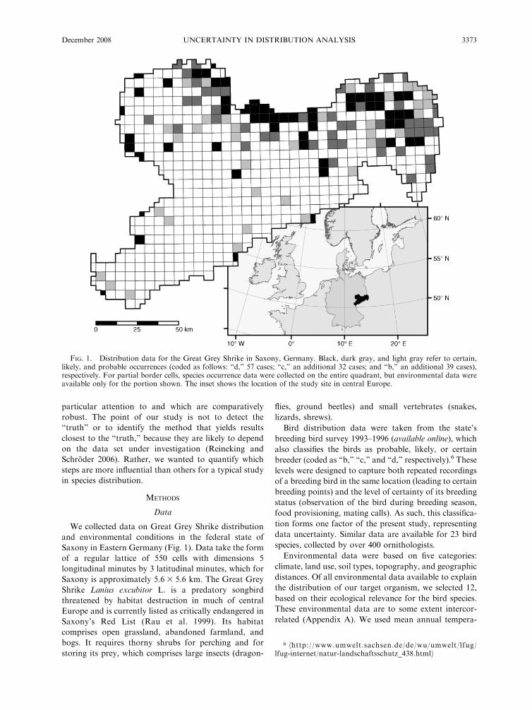
We collected data on Great Grey Shrike distribution
and environmental conditions in the federal state of
Saxony in Eastern Germany (Fig. 1). Data take the form
of a regular lattice of 550 cells with dimensions 5
longitudinal minutes by 3 latitudinal minutes, which for
Saxony is approximately 5.6 3 5.6 km. The Great Grey
Shrike Lanius excubitor L. is a predatory songbird
threatened by habitat destruction in much of central
Europe and is currently listed as critically endangered in
Saxony’s Red List (Rau et al. 1999). Its habitat
comprises open grassland, abandoned farmland, and
bogs. It requires thorny shrubs for perching and for
storing its prey, which comprises large insects (dragon-
flies, ground beetles) and small vertebrates (snakes,
lizards, shrews).
Bird distribution data were taken from the state’s
breeding bird survey 1993–1996 (available online), which
also classifies the birds as probable, likely, or certain
breeder (coded as ‘‘b,’’ ‘‘c,’’ and ‘‘d,’’ respectively).6 These
levels were designed to capture both repeated recordings
of a breeding bird in the same location (leading to certain
breeding points) and the level of certainty of its breeding
status (observation of the bird during breeding season,
food provisioning, mating calls). As such, this classifica-
tion forms one factor of the present study, representing
data uncertainty. Similar data are available for 23 bird
species, collected by over 400 ornithologists.
Environmental data were based on five categories:
climate, land use, soil types, topography, and geographic
distances. Of all environmental data available to explain
the distribution of our target organism, we selected 12,
based on their ecological relevance for the bird species.
These environmental data are to some extent intercor-
related (Appendix A). We used mean annual tempera-
FIG. 1. Distribution data for the Great Grey Shrike in Saxony, Germany. Black, dark gray, and light gray refer to certain,likely, and probable occurrences (coded as follows: ‘‘d,’’ 57 cases; ‘‘c,’’ an additional 32 cases; and ‘‘b,’’ an additional 39 cases),respectively. For partial border cells, species occurrence data were collected on the entire quadrant, but environmental data wereavailable only for the portion shown. The inset shows the location of the study site in central Europe.
6 hhttp://www.umwelt.sachsen.de/de/wu/umwelt/lfug/lfug-internet/natur-landschaftsschutz_438.htmli
December 2008 3373UNCERTAINTY IN DISTRIBUTION ANALYSIS
ture and annual precipitation for the period 1961–1990,
purchased from the Deutscher Wetterdienst as gridded
data (available online).7 The initial resolution of 1 3 1
km was aggregated to that of the bird distribution data
at the expense of slightly reduced value ranges (regres-
sion towards the mean). Land-use variables (percentage
of arable land, bogs, forest, grassland, and unused, poor
open land) were based on 16 000 color-infrared aerial
photographs taken in 1992 and 1993 for the whole of
Saxony and classified into eight main and 40 subcate-
gories (details and data purchasing information are
available online).8 The percentage of sandy soil was also
included as an environmental variable since it charac-
terizes dry and agriculturally less valuable areas (‘‘poor
open’’). Data were taken by merging the forest and the
agriculture soil surveys. Topographical variance was
represented by the variable slope, which is based on the
high-resolution SRTM-3 data (available online).9 Final-
ly, we calculated geographic distances between each
cell’s center, the nearest settlement, and the nearest river
or lake.
All environmental variables were transformed to
achieve an even spread across the data range. Specifi-
cally, slope, percentage arable, forest, grassland, and
sandy soil were square-root transformed, while the
percentage of poor open land, distances to river and
settlement, and mean summer precipitation and temper-
ature were log(x þ c)-transformed (where c equals half
the smallest nonzero value). Finally, all transformed
environmental data were standardized to a mean of 0
and standard deviation of 1.
Climate scenarios were provided by Meteo-Research
(available online).10 Projections from the regional climate
model WETTREG based on global simulations from
the ECHAM5-Model were taken for the decade from
2041 to 2050. IPCC-Scenarios A1B, A2, and B1 (IPCC
2001) each with three realizations that reflect a dry, wet,
and normal decade were used (see Methods: Predictions,
scenarios, and realizations for details). Based on a daily
time series for mean summer precipitation and mean
annual temperature for climate stations, values for our
lattice were obtained by external drift kriging using the
R-package geoR and elevation as a covariate.
Statistical modeling approaches
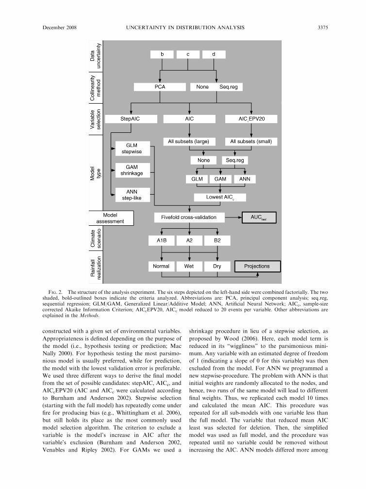
The overall workflow of our study is presented in Fig.
2. We analyzed the contribution of four omnipresent
modeling issues to the overall quality of the model: data
uncertainty, collinearity, model type, and variable
selection. For each step, three alternatives were em-
ployed in a factorial manner, resulting in 34 ¼ 81
different models. Each model was cross-validated
fivefold, i.e., built on 80% of the data (training) and
validated on 20% (test), yielding 405 model runs. In the
analysis of this SDM experiment, we used the cross-
validation model runs as replicates and the mean AUC
(area under curve) value as our response variable.
Collinearity methods.—Of the various methods avail-
able to account for correlated environmental variables,
we selected principal component analysis (PCA; Legen-
dre and Legendre 1998), sequential regression (‘‘seq.reg’’
in Fig. 2; Graham 2003), and no correction. Both PCA
and sequential regression yield orthogonal transformed
variables, but with very different meaning. In PCA, each
principal component reduces the remaining variance in
the matrix of environmental data, and all variables
contribute to all axes. In sequential regression, a
(nonlinear) univariate pre-scan was used to rank
explanatory variables according to their ability to
explain variation in presence-absence data. Then, the
best variable (say ‘‘A’’) remains as it is, while the second-
best (say ‘‘B’’) is regressed against the first, and the
residuals of this regression now represent this second-
best variable (‘‘B*’’). B* must be interpreted as ‘‘the
effect of B in addition to that already explained by A.’’
The same procedure is now repeated for the next
variable (C regressed against A þ B*) and so forth.
Thus, in contrast to PCA, each orthogonal new variable
is represented by one variable only.
The combination of sequential regression and best-
subset regression is rather computer intensive, since
every set of variables must be re-computed whenever a
variable is deleted during stepwise selection (see Fig. 2,
paths below AIC and AICcEPV20). Despite its good
performance in simulation studies (Graham 2003),
sequential regression is seldom used in statistical
analyses. This is mainly due to the conditionality of
residuals and the level of arbitration entering through
the sequence in which variables are considered and
residuals are calculated. Both limitations are of little
relevance to our study since we were mainly interested in
its effect on model quality in general.
Model type.—We selected three model types: Gener-
alized Linear Models (GLM, with logit link and
assuming a binomial error distribution; McCullough
and Nelder 1989), Generalized Additive Models (GAM,
with cubic smoothing splines; Wood 2006) and Artificial
Neural Networks (ANN, feed-forward ANN with one
hidden layer; Venables and Ripley 2002). These methods
performed the best in the comparative study by Pearson
et al. (2006). The hidden layer of the ANN contained
seven units (‘‘nodes’’) and had a weight decay of 0.03,
following the example of Thuiller (2003). All three
model approaches (GLM, GAM, and ANN) allowed for
nonlinear effects (for GLM by including a quadratic
term), but we did not incorporate interactions to limit
computational effort.
Variable selection.—Model selection refers to selecting
the most appropriate model from those that can be
7 hhttp://www.dwd.dei8 hh t t p : / / w w w . u m w e l t . s a c h s e n . d e / l f u g /
natur-landschaftsschutz_328.htmli9 hhttp://edcsgs9.cr.usgs.gov./pub/data/srtmi10 hhttp://www.cec-potsdam.de/Produkte/Klima/WettReg/
wettreg.htmli
CARSTEN F. DORMANN ET AL.3374 Ecology, Vol. 89, No. 12
constructed with a given set of environmental variables.
Appropriateness is defined depending on the purpose of
the model (i.e., hypothesis testing or prediction; Mac
Nally 2000). For hypothesis testing the most parsimo-
nious model is usually preferred, while for prediction,
the model with the lowest validation error is preferable.
We used three different ways to derive the final model
from the set of possible candidates: stepAIC, AICc, and
AICcEPV20 (AIC and AICc were calculated according
to Burnham and Anderson 2002). Stepwise selection
(starting with the full model) has repeatedly come under
fire for producing bias (e.g., Whittingham et al. 2006),
but still holds its place as the most commonly used
model selection algorithm. The criterion to exclude a
variable is the model’s increase in AIC after the
variable’s exclusion (Burnham and Anderson 2002,
Venables and Ripley 2002). For GAMs we used a
shrinkage procedure in lieu of a stepwise selection, as
proposed by Wood (2006). Here, each model term is
reduced in its ‘‘wiggliness’’ to the parsimonious mini-
mum. Any variable with an estimated degree of freedom
of 1 (indicating a slope of 0 for this variable) was then
excluded from the model. For ANN we programmed a
new stepwise-procedure. The problem with ANN is that
initial weights are randomly allocated to the nodes, and
hence, two runs of the same model will lead to different
final weights. Thus, we replicated each model 10 times
and calculated the mean AIC. This procedure was
repeated for all sub-models with one variable less than
the full model. The variable that reduced mean AIC
least was selected for deletion. Then, the simplified
model was used as full model, and the procedure was
repeated until no variable could be removed without
increasing the AIC. ANN models differed more among
FIG. 2. The structure of the analysis experiment. The six steps depicted on the left-hand side were combined factorially. The twoshaded, bold-outlined boxes indicate the criteria analyzed. Abbreviations are: PCA, principal component analysis; seq.reg,sequential regression; GLM/GAM, Generalized Linear/Additive Model; ANN, Artificial Neural Network; AICc, sample-sizecorrected Akaike Information Criterion; AICcEPV20, AICc model reduced to 20 events per variable. Other abbreviations areexplained in the Methods.
December 2008 3375UNCERTAINTY IN DISTRIBUTION ANALYSIS
repeated runs than GLM or GAM, making the selection
of variables for the ‘‘best’’ model less reproducible. Since
their success in predictive models has often been hailed
(Hilbert and Ostendorf 2001, Recknagel 2001, Thuiller
2003, Segurado and Araujo 2004, Araujo et al. 2005), we
still kept this method.
For small sample sizes, the sample size-corrected AICc
was proposed (Burnham and Anderson 2002), which
was implemented in the other two model selection
procedures: We constructed all possible subsets of
variables (with and without quadratic terms). This all-
subsets approach was used in two flavors: In ‘‘AICc,’’ the
model with the lowest AICc value is returned, up to a
model complexity of 12 variables (see Whittingham et al.
2007, for a similar implementation). In AICcEPV20, we
additionally restricted the set of possible candidates to
those models having a maximum of N/20 parameters
(where N is the minimum of number of presences or
absences in the data set). Harrell (2001) refers to this
value as events-per-variable (EPV). An EPV of 20
generally leads to small and robust models.
Reference analyses
In our analysis we ran hundreds of thousands of
models. By chance alone there may be very well-fitting
ones among them. Therefore, we decided to carry out
two different reference analyses: a null model and a best-
possible model.
The null model consisted of the same response
variables (i.e., the presence–absence value observed with
data uncertainty probable, likely, or certain breeder,
coded as ‘‘b,’’ ‘‘c,’’ and ‘‘d,’’ respectively), but the 12
environmental variables are replaced by random values.
It addressed the view that, with high-computational
approaches, one may only be ‘‘fishing for significance.’’
We decided to retain the correlation structure of the
original variables, because this constrains the model
space. Hence, the 12 new random environmental
variables were drawn from a multi-normal distribution
with means ¼ 0 and standard deviation ¼ 1 (i.e., values
are normalized, as are the original environmental data),
and with a correlation matrix defined by the observed
correlation matrix. Then, we also repeated the fivefold
cross-validation analysis as described in the Methods:
Analysis section for the null model in order to estimate
the model quality of a random environment without
ecological meaning.
The best-possible model is aimed at defining the upper
limit of what the models can possibly achieve. For this
approach, we constructed a simple virtual species (e.g.,
Meynard and Quinn 2007), whose presence–absence
data are fully determined by the environmental values.
We used a complex, but ecological plausible functional
relationship between four environmental variables to
predict the occurrence probability for the virtual species,
which was guided by a preliminary GLM analysis: g(p)
¼ 75 – (1.63biotope diversity) – (63distance to river)þ(0.5 3 percentage low quality open land) þ 0.1(percent-
age of low quality open land)2 – (0.5 3 annual
precipitation) þ (0.2 3 annual precipitation�distance to
river), where g ¼ ln(p/(1 – p)) is the logit-link function,
and p is occurrence probability. This equation was
derived by first specifying the four environmental
variables we deemed ecologically plausible, then speci-
fying a regression model including a quadratic term and
an interaction, and then fitting this pre-specified model
to the real data using a GLM. The estimated coefficients
were then used to construct the virtual species. In this
way, our virtual species carries the characteristics of our
expectation and our data, without being a replicate of
any observed data. For each level of data uncertainty, a
threshold level was chosen to convert probabilities into
0/1 in such a way as to match the observed prevalences.
Analyzing this data set in the same way as the observed
data, we could quantify the ability of model approaches
to detect the true underlying explanatory variables.
Since the results from these two models satisfied our
underlying assumptions, we only briefly present them in
this section and do not return to them in the Results or
Discussion. In brief, they show that for the null model
test, all AUC values were very poor and in fact
indistinguishable from pure chance ¼ 0.5 (mean 6 SD
AUC across the five validation runs of all 81 models,
0.495 6 0.030). For the virtual species, the mean AUC
was 0.956 6 0.036 and hence excellent. These findings
show that our approach (1) was not biased by detecting
irrelevant variables and (2) can, at least in principle,
model the correct underlying relationship independent
of model type with very high precision.
Predictions, scenarios, and realizations
Species distribution models are often used to assess
the effect of environmental change on species distribu-
tions, by forecasting (projecting) occurrence probabili-
ties to future scenarios. We employed three different
scenarios (A1B, A2, and B2, following the IPCC Special
Report on Emissions Scenarios [SRES], where A1B
represents global convergence and rapid economic
growth with balanced use of energy sources; A2
represents regional development and slower economic
growth; B2 refers to an emphasis on local to regional
development, with slower economic growth and higher
levels of environmental protection). For each of these
three climate change scenarios, we chose three different
realizations for precipitation trends, since rainfall can be
predicted only with high uncertainty: dry, average, wet.
As it turns out, scenarios mainly represented tempera-
ture increases (approximately 17%, 19%, and 17% of the
current annual average of 8.28C), while realizations
within scenarios differed mainly in summer precipitation
(approximately�9%, 0%, andþ2% change compared to
today’s 220 mm, respectively).
Onto each of these nine scenario–realizations we
projected occurrence probabilities using the 81 different
models, now built on the full data set, resulting in 729
projections. A confusion matrix was generated that
CARSTEN F. DORMANN ET AL.3376 Ecology, Vol. 89, No. 12
cross-tabulated observed and predicted occurrence
patterns in true/false presences and absences: a repre-
sents presences observed and predicted; b observed but
not predicted presences; c predicted but not observed
presences; and d predicted and observed absences
(Fielding and Bell 1997). To derive the values for a to
d for the present species distribution, we used different
thresholds to convert the occurrence probability given
by the model fit into presence-absence data. Firstly,
when we are interested in the change of species
prevalence, the threshold should be chosen in such a
way that fitted model data and observed data have the
same number of predicted occurrences (‘‘prevalence
constancy’’; (aþb)/(aþ c)). Secondly, we were interested
in geographical shifts of the distribution; hence, for this
measure the threshold should be chosen to match
observed and fitted values most closely (‘‘location
constancy,’’ b/(a þ b)). Finally, we may want to
maximize the agreement of model fit and observations
for presences and absences, which can be achieved using
kappa maximization (see Fielding and Bell 1997 for
formula). Prevalence constancy and kappa maximiza-
tion yielded similar thresholds (mean across all 81
models of 0.341 and 0.334, respectively), but location
constancy led to rather different values (0.705).
For scenario projections we used the different
thresholds computed for the full model. We then
calculated changes in species occurrence (using the
‘‘prevalence constancy’’ formula) and shifts in their
locations (using the ‘‘location constancy’’ formula) due
to climate change. These values were then analyzed for
the main drivers: model-building steps and scenario/re-
alizations.
Analysis
The SDM experiment delivered data from 81 different
model approaches, ‘‘replicated’’ across the five valida-
tion data sets. Since these ‘‘replicates’’ shared 20%–80%
of the same data, they cannot be considered indepen-
dently. We thus analyzed the mean AUC values across
the five validation runs by means of analysis of variance.
Model diagnostics showed that residuals were approx-
imately normally distributed and variances homoge-
nous.
Analysis of variance calculates the variance (in terms
of sum of squares) that can be attributed to each step in
the model sequence, which represent the factors of the
experiment. Hierarchical partitioning (Chevan and
Sutherland 1991, Mac Nally 2000) was used to rank
the importance of the main factors. Although some
interactions were significant in ANOVA, these contrib-
uted little to the variation explained, and hence a
ranking of the main factors seemed acceptable. Similar-
ly, we analyzed the variation in predicted changes in
prevalence and shifts of the distribution for the 729
projections for the effect of the six explanatory variables
(the four modeling steps plus the two scenario steps). All
analyses were carried out using the free software R (R
Development Core Team 2008) versions 2.3.1–2.6.0,
with packages MASS, nnet, geoR, gtools, mgcv, multi-
comp and verification (Venables and Ripley 2002).
RESULTS
We present the findings of our analysis in the
following sections. First, we analyze the effect of data
uncertainty, model type, variable selection method, and
collinearity correction on the models ability to discrim-
inate between presences and absences (as measured by
the mean AUC of five subsets for the 80/20 cross-
validation). This produced the main picture of which the
model-building steps were particularly important in our
analysis. Secondly, we investigate whether the different
modeling approaches identify the same environmental
variables as important for the distribution of the Great
Grey Shrike. Thirdly, we used the models built on the
full data set to predict the species distribution under nine
different climate change scenarios. Here we analyze the
change in prevalence and the shift of distributions under
the 81 models and 9 scenarios (729 projections).
Variation introduced by model-building steps
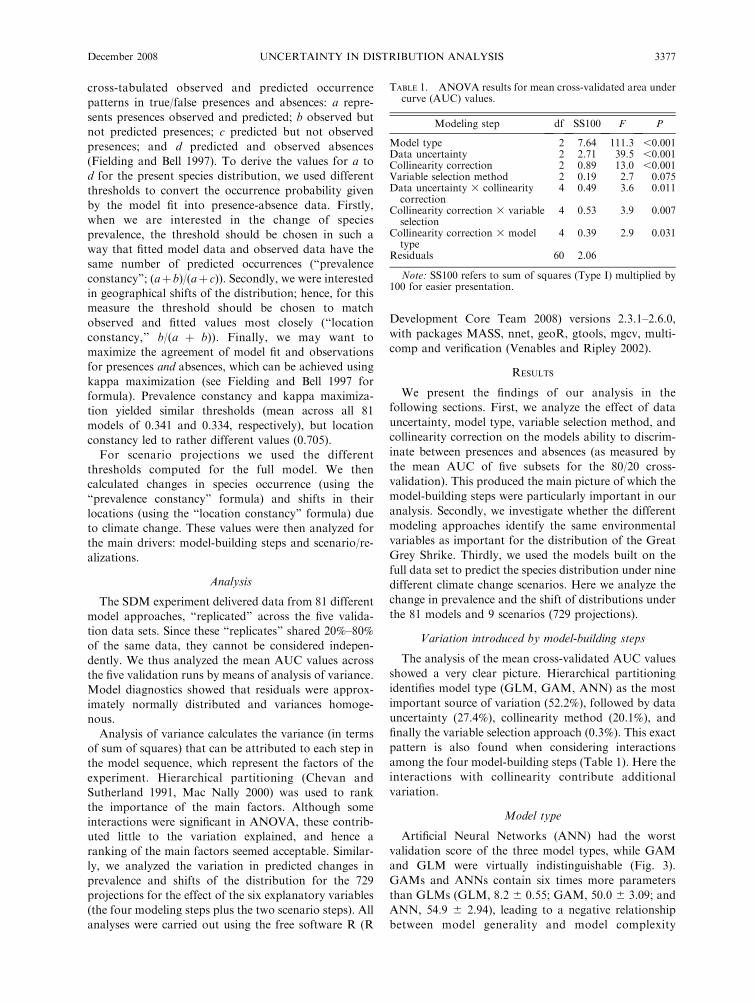
The analysis of the mean cross-validated AUC values
showed a very clear picture. Hierarchical partitioning
identifies model type (GLM, GAM, ANN) as the most
important source of variation (52.2%), followed by data
uncertainty (27.4%), collinearity method (20.1%), and
finally the variable selection approach (0.3%). This exact
pattern is also found when considering interactions
among the four model-building steps (Table 1). Here the
interactions with collinearity contribute additional
variation.
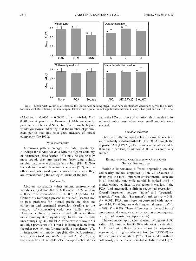
Model type
Artificial Neural Networks (ANN) had the worst
validation score of the three model types, while GAM
and GLM were virtually indistinguishable (Fig. 3).
GAMs and ANNs contain six times more parameters
than GLMs (GLM, 8.2 6 0.55; GAM, 50.0 6 3.09; and
ANN, 54.9 6 2.94), leading to a negative relationship
between model generality and model complexity
TABLE 1. ANOVA results for mean cross-validated area undercurve (AUC) values.
Modeling step df SS100 F P
Model type 2 7.64 111.3 ,0.001Data uncertainty 2 2.71 39.5 ,0.001Collinearity correction 2 0.89 13.0 ,0.001Variable selection method 2 0.19 2.7 0.075Data uncertainty 3 collinearity
correction4 0.49 3.6 0.011
Collinearity correction 3 variableselection
4 0.53 3.9 0.007
Collinearity correction 3 modeltype
4 0.39 2.9 0.031
Residuals 60 2.06
Note: SS100 refers to sum of squares (Type I) multiplied by100 for easier presentation.
December 2008 3377UNCERTAINTY IN DISTRIBUTION ANALYSIS
(AUCpred ¼ 0.80004 – 0.00086 df, r ¼ �0.461, P ,
0.001; see Appendix B). However, GAMs are equally
parameter rich as ANNs, but have much higher
validation scores, indicating that the number of param-
eters per se may not be a good measure of model
complexity (Ye 1998).
Data uncertainty
A curious pattern emerges for data uncertainty.
Although the models for data with the highest certainty
of occurrence (classification ‘‘d’’) may be ecologically
most sound, they are based on fewer data points,
making parameter estimation less robust (Fig. 3). Too
lax a definition of a breeding occurrence (‘‘b’’), on the
other hand, also yields poorer model fits, because they
are overestimating the ecological niche of the bird.
Collinearity
Absolute correlation values among environmental
variables ranged from 0.01 to 0.91 (mean¼ 0.29, median
¼ 0.25; four correlations jrj . 0.6; Appendix A).
Collinearity (although present in our data) seemed not
to pose problems for internal prediction, since no
correction and sequential regression (leading to the
removal of collinearity) yield very similar results.
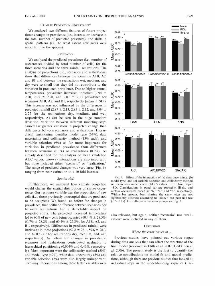
However, collinearity interacts with all other three
model-building steps significantly. In the case of data
uncertainty (Fig. 4a), the PCA works worse at low (‘‘b’’)
and high prevalence (‘‘d’’), but is indistinguishable from
the other two methods for intermediate prevalence (‘‘c’’).
In interaction with model type (Fig. 4b), PCA performs
worse with GAM and ANN than with GLM. Finally,
the interaction of variable selection approaches shows
again the PCA as source of variation, this time due to its
reduced robustness when very small models were
selected.
Variable selection
The three different approaches to variable selection
were virtually indistinguishable (Fig. 3). Although the
approach AICcEPV20 yielded somewhat smaller models
than the other two, validation AUC values were very
similar.
ENVIRONMENTAL CORRELATES OF GREAT GREY
SHRIKE DISTRIBUTION
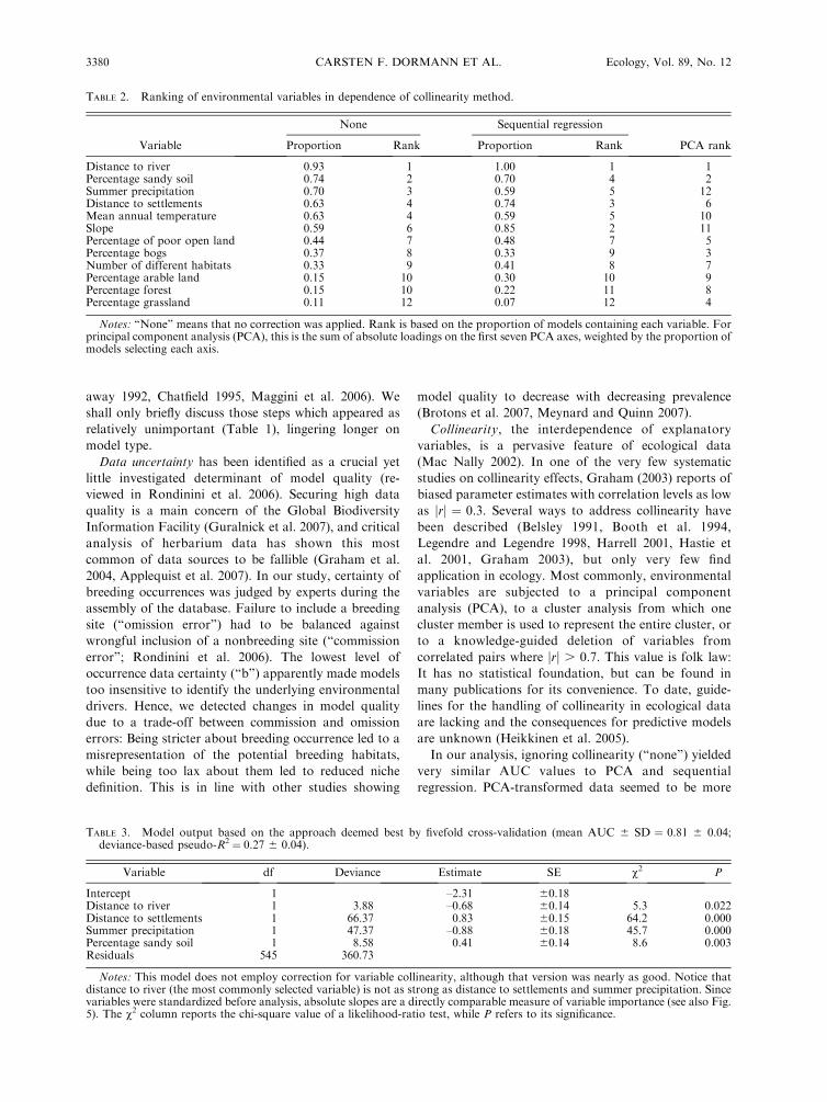
Variable importance differed depending on the
collinearity method employed (Table 2). Distance to
rivers was the most important environmental correlate
in all methods, but, while rainfall is ranked third in
models without collinearity correction, it was last in the
PCA (and intermediate fifth in sequential regression).
Overall agreement between ‘‘none’’ and ‘‘sequential
regression’’ was high (Spearman’s rank test: q ¼ 0.88,
P , 0.001), PCA ranks were not correlated with ‘‘none’’
(q¼ 0.14, P¼ 0.66), nor with ‘‘sequential regression’’ (q¼ 0.09, P ¼ 0.78). These differences in the ranking of
environmental variables must be seen as a consequence
of their collinearity (see Appendix A).
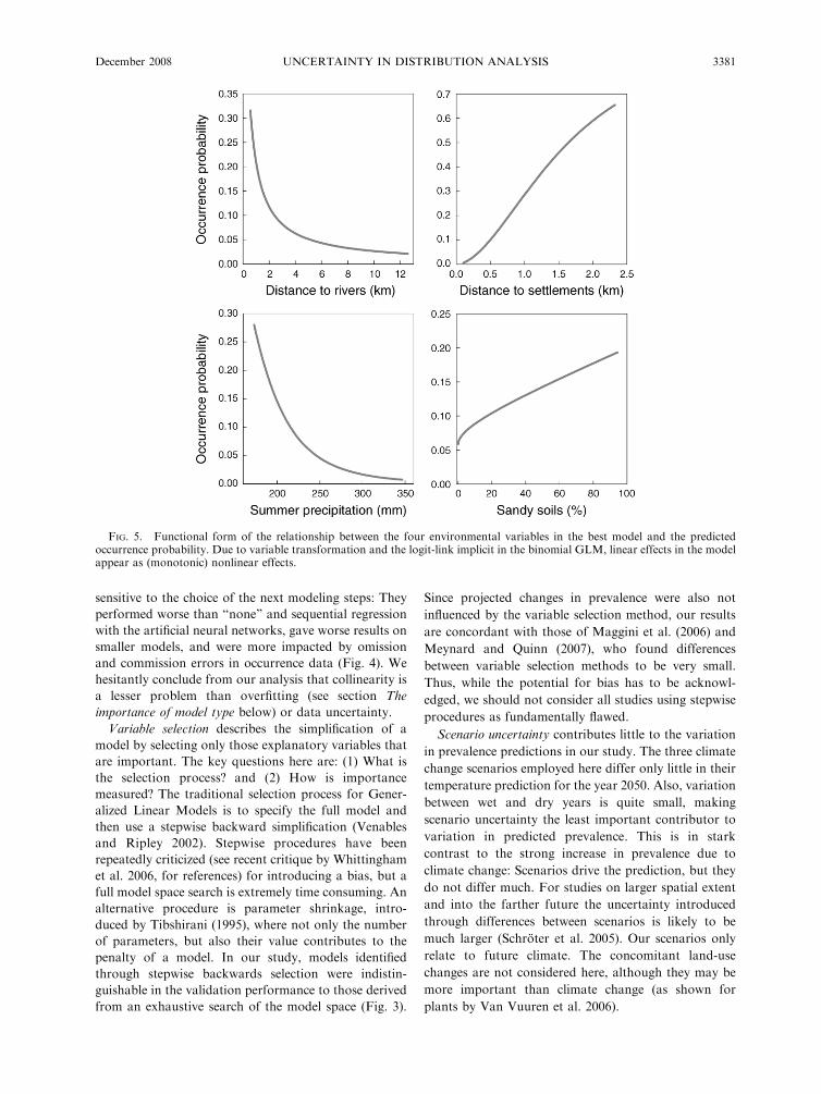
The two model approaches sharing the highest AUC
value (0.83, based on five 80/20 validations) is a standard
GLM without collinearity correction (or sequential
regression), strong variable selection (AICcEPV20) for
the medium certain data (‘‘c’’). This model without
collinearity correction is presented in Table 3 and Fig. 5.
FIG. 3. Mean AUC values as affected by the four model-building steps. Error bars are standard deviations across the 27 runsfor each level. Bars sharing the same capital letter within a panel are not significantly different (Tukey’s hsd post hoc test P . 0.05).
CARSTEN F. DORMANN ET AL.3378 Ecology, Vol. 89, No. 12
CLIMATE PROJECTION UNCERTAINTY
We analyzed two different features of future projec-
tions: changes in prevalence (i.e., increase or decrease inthe total number of predicted presences), and shifts inspatial patterns (i.e., to what extent new areas were
important for the species).
Prevalence
We analyzed the predicted prevalence (i.e., number of
occurrences divided by total number of cells) for thethree scenarios and the three rainfall realizations. The
analysis of projections (i.e., scenarios and realizations)show that differences between the scenarios A1B, A2,
and B1 and between the realizations wet, medium, anddry were so small that they did not contribute to the
variation in predicted prevalence. Due to higher annualtemperatures, prevalence increased threefold (2.94 6
2.20, 2.95 6 2.20, and 2.87 6 2.13 prevalence forscenarios A1B, A2, and B1, respectively [mean 6 SD]).
This increase was not influenced by the differences inpredicted rainfall (2.87 6 2.13, 2.85 6 2.12, and 3.04 6
2.27 for the realizations dry, medium, and wet,respectively). As can be seen in the huge standarddeviation, variation between different modeling steps
caused far greater variation in projected change thandifferences between scenarios and realizations. Hierar-
chical partitioning identifies model type (63%), datauncertainty and collinearity method (13% each), and
variable selection (9%) as far more important forvariation in predicted prevalence than differences
between scenarios (0.1%) or realizations (0.9%). Asalready described for the analysis of mean validation
AUC values, two-way interactions are also important,but none included either ‘‘scenario’’ or ‘‘realization.’’
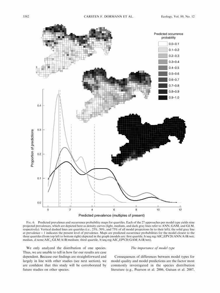
The range of predicted changes was very large (Fig. 6),ranging from near-extinction to a 10-fold increase.
Spatial shift
Furthermore, we analyzed how climate projectionwould change the spatial distribution of shrike occur-
rence. Our response variable was the proportion of newcells (i.e., those previously unoccupied that are predictedto be occupied). We found, as before for changes in
prevalence, that neither difference between scenarios norbetween realizations had a detectable impact on
projected shifts. The projected increased temperatureled to 60% of new cells being occupied (60.4 % 6 28.3%,
60.7% 6 28.2%, and 60.4% 6 27.8%, for A1B, A2, andB1, respectively). Differences in predicted rainfall were
irrelevant in these projections (59.8 6 28.1, 59.6 6 28.3,and 62.0627.7 for realizations dry, medium, and wet,
respectively). As before for changes in prevalence,scenarios and realizations contributed negligibly to
hierarchical partitioning (0.004% and 0.46%, respective-ly). Most important were the collinearity method (50%)
and model type (42%), while data uncertainty (5%) andvariable selection (2%) were also largely unimportant.
Two-way interactions among these latter variables were
also relevant, but again, neither ‘‘scenario’’ nor ‘‘reali-
zation’’ were included in any of them.
DISCUSSION
Where the error comes in . . .
Previous studies have pointed out various stages
during data analysis that can affect the structure of the
final model (reviewed in Elith et al. 2002, Heikkinen et
al. 2006). The present study is the first to quantify the
relative contributions on model fit and model predic-
tions, although there are previous studies that looked at
individual steps in the model-building sequence (Far-
FIG. 4. Effect of the interaction of (a) data uncertainty, (b)model type, and (c) variable selection and collinearity methodon mean area under curve (AUC) values. Error bars depictþSD. Classifications in panel (a) are probable, likely, andcertain occurrences coded as ‘‘b,’’ ‘‘c,’’ and ‘‘d,’’ respectively.Within bar groups, bars sharing the same letter are notsignificantly different according to Tukey’s hsd post hoc test(P . 0.05). For differences between groups see Fig. 3.
December 2008 3379UNCERTAINTY IN DISTRIBUTION ANALYSIS
away 1992, Chatfield 1995, Maggini et al. 2006). We
shall only briefly discuss those steps which appeared as
relatively unimportant (Table 1), lingering longer on
model type.
Data uncertainty has been identified as a crucial yet
little investigated determinant of model quality (re-
viewed in Rondinini et al. 2006). Securing high data
quality is a main concern of the Global Biodiversity
Information Facility (Guralnick et al. 2007), and critical
analysis of herbarium data has shown this most
common of data sources to be fallible (Graham et al.
2004, Applequist et al. 2007). In our study, certainty of
breeding occurrences was judged by experts during the
assembly of the database. Failure to include a breeding
site (‘‘omission error’’) had to be balanced against
wrongful inclusion of a nonbreeding site (‘‘commission
error’’; Rondinini et al. 2006). The lowest level of
occurrence data certainty (‘‘b’’) apparently made models
too insensitive to identify the underlying environmental
drivers. Hence, we detected changes in model quality
due to a trade-off between commission and omission
errors: Being stricter about breeding occurrence led to a
misrepresentation of the potential breeding habitats,
while being too lax about them led to reduced niche
definition. This is in line with other studies showing
model quality to decrease with decreasing prevalence
(Brotons et al. 2007, Meynard and Quinn 2007).
Collinearity, the interdependence of explanatory
variables, is a pervasive feature of ecological data
(Mac Nally 2002). In one of the very few systematic
studies on collinearity effects, Graham (2003) reports of
biased parameter estimates with correlation levels as low
as jrj ¼ 0.3. Several ways to address collinearity have
been described (Belsley 1991, Booth et al. 1994,
Legendre and Legendre 1998, Harrell 2001, Hastie et
al. 2001, Graham 2003), but only very few find
application in ecology. Most commonly, environmental
variables are subjected to a principal component
analysis (PCA), to a cluster analysis from which one
cluster member is used to represent the entire cluster, or
to a knowledge-guided deletion of variables from
correlated pairs where jrj . 0.7. This value is folk law:
It has no statistical foundation, but can be found in
many publications for its convenience. To date, guide-
lines for the handling of collinearity in ecological data
are lacking and the consequences for predictive models
are unknown (Heikkinen et al. 2005).
In our analysis, ignoring collinearity (‘‘none’’) yielded
very similar AUC values to PCA and sequential
regression. PCA-transformed data seemed to be more
TABLE 2. Ranking of environmental variables in dependence of collinearity method.
Variable
None Sequential regression
PCA rankProportion Rank Proportion Rank
Distance to river 0.93 1 1.00 1 1Percentage sandy soil 0.74 2 0.70 4 2Summer precipitation 0.70 3 0.59 5 12Distance to settlements 0.63 4 0.74 3 6Mean annual temperature 0.63 4 0.59 5 10Slope 0.59 6 0.85 2 11Percentage of poor open land 0.44 7 0.48 7 5Percentage bogs 0.37 8 0.33 9 3Number of different habitats 0.33 9 0.41 8 7Percentage arable land 0.15 10 0.30 10 9Percentage forest 0.15 10 0.22 11 8Percentage grassland 0.11 12 0.07 12 4
Notes: ‘‘None’’ means that no correction was applied. Rank is based on the proportion of models containing each variable. Forprincipal component analysis (PCA), this is the sum of absolute loadings on the first seven PCA axes, weighted by the proportion ofmodels selecting each axis.
TABLE 3. Model output based on the approach deemed best by fivefold cross-validation (mean AUC 6 SD ¼ 0.81 6 0.04;deviance-based pseudo-R2 ¼ 0.27 6 0.04).
Variable df Deviance Estimate SE v2 P
Intercept 1 –2.31 60.18Distance to river 1 3.88 –0.68 60.14 5.3 0.022Distance to settlements 1 66.37 0.83 60.15 64.2 0.000Summer precipitation 1 47.37 –0.88 60.18 45.7 0.000Percentage sandy soil 1 8.58 0.41 60.14 8.6 0.003Residuals 545 360.73
Notes: This model does not employ correction for variable collinearity, although that version was nearly as good. Notice thatdistance to river (the most commonly selected variable) is not as strong as distance to settlements and summer precipitation. Sincevariables were standardized before analysis, absolute slopes are a directly comparable measure of variable importance (see also Fig.5). The v2 column reports the chi-square value of a likelihood-ratio test, while P refers to its significance.
CARSTEN F. DORMANN ET AL.3380 Ecology, Vol. 89, No. 12
sensitive to the choice of the next modeling steps: They
performed worse than ‘‘none’’ and sequential regression
with the artificial neural networks, gave worse results on
smaller models, and were more impacted by omission
and commission errors in occurrence data (Fig. 4). We
hesitantly conclude from our analysis that collinearity is
a lesser problem than overfitting (see section The
importance of model type below) or data uncertainty.
Variable selection describes the simplification of a
model by selecting only those explanatory variables that
are important. The key questions here are: (1) What is
the selection process? and (2) How is importance
measured? The traditional selection process for Gener-
alized Linear Models is to specify the full model and
then use a stepwise backward simplification (Venables
and Ripley 2002). Stepwise procedures have been
repeatedly criticized (see recent critique by Whittingham
et al. 2006, for references) for introducing a bias, but a
full model space search is extremely time consuming. An
alternative procedure is parameter shrinkage, intro-
duced by Tibshirani (1995), where not only the number
of parameters, but also their value contributes to the
penalty of a model. In our study, models identified
through stepwise backwards selection were indistin-
guishable in the validation performance to those derived
from an exhaustive search of the model space (Fig. 3).
Since projected changes in prevalence were also not
influenced by the variable selection method, our results
are concordant with those of Maggini et al. (2006) and
Meynard and Quinn (2007), who found differences
between variable selection methods to be very small.
Thus, while the potential for bias has to be acknowl-
edged, we should not consider all studies using stepwise
procedures as fundamentally flawed.
Scenario uncertainty contributes little to the variation
in prevalence predictions in our study. The three climate
change scenarios employed here differ only little in their
temperature prediction for the year 2050. Also, variation
between wet and dry years is quite small, making
scenario uncertainty the least important contributor to
variation in predicted prevalence. This is in stark
contrast to the strong increase in prevalence due to
climate change: Scenarios drive the prediction, but they
do not differ much. For studies on larger spatial extent
and into the farther future the uncertainty introduced
through differences between scenarios is likely to be
much larger (Schroter et al. 2005). Our scenarios only
relate to future climate. The concomitant land-use
changes are not considered here, although they may be
more important than climate change (as shown for
plants by Van Vuuren et al. 2006).
FIG. 5. Functional form of the relationship between the four environmental variables in the best model and the predictedoccurrence probability. Due to variable transformation and the logit-link implicit in the binomial GLM, linear effects in the modelappear as (monotonic) nonlinear effects.
December 2008 3381UNCERTAINTY IN DISTRIBUTION ANALYSIS
We only analyzed the distribution of one species.
Thus, we are unable to tell in how far our results are case
dependent. Because our findings are straightforward and
largely in line with other studies (see next section), we
are confident that this study will be corroborated by
future studies on other species.
The importance of model type
Consequences of differences between model types for
model quality and model predictions are the factor most
commonly investigated in the species distribution
literature (e.g., Pearson et al. 2006, Guisan et al. 2007,
FIG. 6. Predicted prevalence and occurrence probability maps for quartiles. Each of the 27 approaches per model type yields nineprojected prevalences, which are depicted here as density curves (light, medium, and dark gray lines refer to ANN, GAM, and GLM,respectively). Vertical dashed lines are quartiles (i.e., 25%, 50%, and 75% of all model projections lie to their left); the solid gray lineat prevalence¼ 1 indicates the present level of prevalence. Maps are predicted occurrence probabilities for the model closest to thethree quartiles (from top left to bottom right) depicted in the graph (models are: first quartile, b/seq.reg/AICcEPV20/ANN/A1B/wet;median, d/none/AICc/GLM/A1B/medium; third quartile, b/seq.reg/AICcEPV20/GAM/A1B/wet).
CARSTEN F. DORMANN ET AL.3382 Ecology, Vol. 89, No. 12
Meynard and Quinn 2007). Since these findings have
not, to our knowledge, been synthesized into clear
recommendations, we will briefly go into some more
detail here.
Model types fall largely into three groups: ‘‘tradition-
al’’ approaches such as Generalized Linear Models
(GLM), Generalized Additive Models (GAM), Discrim-
inant Analysis, Classification And Regression Trees
(CART); ‘‘machine-learning’’ methods such as Artificial
Neural Networks (ANN), Boosted Regression Trees
(BRT), randomForest, Multiple Adaptive Regression
Splines, Support Vector Machines, and nameless others;
and, thirdly, ‘‘presence-only’’ techniques such as Genetic
Algorithm and Rule-set Prediction, Maximum Entropy,
Environmental Niche Factor Analysis, and various
flavors of bioclimatic envelopes. In comparisons of
presence-only and traditional approaches using pres-
ence–absence data, the latter were generally superior
(e.g., Brotons et al. 2004, Meynard and Quinn 2007).
This comparison is slightly unfair, since presence-only
models come into their own when exposed to presence-
only data, where the other methods are simply not
applicable. Studies comparing traditional and machine-
learning model types (e.g., Segurado and Araujo 2004,
Pearson et al. 2006, Guisan et al. 2007, Meynard and
Quinn 2007) show a very mixed picture: GAM, and,
surprisingly, GLM are usually among the most robust
methods (assessed similar to our study as AUC on a test
data set). Some machine-learning methods give evidence
of a real improvement (particularly Boosted Regression
Trees and the new BRUTO-version of GAMs), but
others exhibit signs of overfitting, i.e., low validation
AUC values (e.g., ANN, GARP, bioclimatic envelopes,
CART, but see Olden and Jackson 2002, for a case of
superior ANN performance). A comparison of methods
‘‘only’’ recently developed, the study of Elith et al. (2006)
shows the full scatter of model qualities.
In our study, the two traditional methods outper-
formed the machine-learning algorithm. Model com-
plexity, expressed in number of parameters fitted,
indicates that more complex models are also more
prone to overfitting (Hastie et al. 2001). The comparison
of GAM and ANN (Appendix B) indicates that this
need not be the case. Rather than number of parameter
per se, it is the flexibility with which these are actually
calculated that determines the tendency of a model to
overfit (‘‘effective number of parameters’’ sensu Hastie
et al. 2001; and ‘‘generalized degrees of freedom’’ in the
words of Ye 1998 and Elder 2003).
It is worth investing time in the selection of a robust
and trustworthy model type. In our study, even
relatively small differences in validation robustness
(Fig. 3) led to huge differences in predicted effects of
climate change (Fig. 6): The hyper-flexible ANN was
most conservative, while the relatively rigid GLM
projects the largest change (Appendix C). Also, ANN
interacted noticeably with the collinearity method (Fig.
4), again cautioning us against its use.
Extensions of this approach
Out of necessity, our study was unable to investigatethe realm of modeling decisions exhaustively. Encour-
agingly, however, each step we investigated mainlycontributed to the model quality variation independent-
ly. Table 1 indicates that the collinearity interactionscontribute only half of data uncertainty and one-fourth
of model type uncertainty. This means that in order toinvestigate the importance of modeling decisions we may
not need to go for full factorial designs such as ours, butcan possibly restrict efforts to univariate explorations
(such as Scott et al. 2002, Maggini et al. 2006). We cansee four immediate ways to extend our study: (1)
incorporate different explanatory variable pre-selections(e.g., expert knowledge, cluster-representatives, pre-
screening); (2) incorporate more of the other possiblemodel types (as mentioned in the section The importance
of model type); (3) incorporate different ways to dealwith spatial autocorrelation (as reviewed in Dormann etal. 2007); and (4) incorporate interactions among
variables (as strongly advocated in Austin et al. 1990,Barry and Elith 2006). Moreover, using an artificial
species approach (advocated by Austin et al. [2006] andcarried out by Hirzel et al. [2001], Mikusinski and
Edenius [2006] and Meynard and Quinn [2007]) wouldadditionally allow to quantify the bias in model fits
introduced by different model steps.
The shrike’s future
Our study’s main aim was to quantify the contribu-
tion of different steps in the model-building procedurefor model quality and climate change projections. But
our results obviously also have bearing on the predictionof the future distribution and prevalence of the Great
Grey Shrike in Saxony. More than 75% of projectedprevalences across all analyses and scenarios are abovethe present prevalence (Fig. 6). Trusting GAM and
GLM more than ANN, we even venture the predictionthat the Great Grey Shrike will thrive under Saxony’s
future climatic conditions. By how much its prevalencewill increase, is, however, burdened with uncertainty.
The inter-quartile range stretches from 1 to 4, with amedian of 2, but even a six-fold increase in prevalence
would still seem statistically plausible (;1/10 of allpredictions are higher than this value). Our prediction
uncertainty compares favorably to the study of Pearsonet al. (2006), who reported a variability from 92% loss to
322% gain for four South African proteacean plantspecies.
Models can fit extremely well but still project poorly,as seen in the case of the sister species, the Red-backed
Shrike (Araujo and Rahbek 2006). Also in the Mediter-ranean, another congener, the Lesser Grey Shrike, has
been decreasing over the last decades (Giralt and Valera2007). So, apart from data, model-building, andscenario uncertainty, additional ecological facets of
uncertainty enter the framework: Will the bird colonizeall suitable sites (e.g., Midgley et al. 2006)? Will the
December 2008 3383UNCERTAINTY IN DISTRIBUTION ANALYSIS
limiting factors remain the same and our models’
assumption of stationarity hold (e.g., Schroder and
Richter 1999, Randin et al. 2006)? Did we manage to
capture all important determinants of the shrike’s
distribution, either as direct effects or at least as proxies
(see Coudun et al. 2006, Luoto et al. 2006, for example,
where inclusion soil and land-use variables made a large
difference to the climate-only models)? In short: Based
on the available data, the future for the Great Grey
Shrike looks bright in Saxony; but we would be very
diffident to stake our reputation on this prediction.
ACKNOWLEDGMENTS
First and foremost, we thank the numerous volunteers who,through their field observations, allowed the compilation of thedatabase underlying the bird distribution data. Secondly, wethank the Sachsische Landesamt fur Umwelt which made thesedata available on the Internet. Finally, our thanks go to BerndGruber and Vanessa Stauch, who discussed various stages ofthis research, and to two anonymous referees who helpedimprove a previous version of this manuscript.
LITERATURE CITED
Applequist, W. L., D. J. McGlinn, M. Miller, Q. G. Long, andJ. S. Miller. 2007. How well do herbarium data predict thelocation of present populations? A test using Echinaceaspecies in Missouri. Biodiversity and Conservation 16:1397–1407.
Araujo, M. B., and A. Guisan. 2006. Five (or so) challenges forspecies distribution modelling. Journal of Biogeography 33:1677–1688.
Araujo, M. B., R. G. Pearson, W. Thuiller, and M. Erhard.2005. Validation of species-climate impact models underclimate change. Global Change Biology 11:1504–1513.
Araujo, M. B., and C. Rahbek. 2006. How does climate changeaffect biodiversity? Science 313:1396–1397.
Austin, M. P. 2002. Spatial prediction of species distribution:an interface between ecological theory and statisticalmodelling. Ecological Modelling 157:101–118.
Austin, M. 2007. Species distribution models and ecologicaltheory: a critical assessment and some possible newapproaches. Ecological Modelling 200:1–19.
Austin, M. P., L. Belbin, J. A. Meyers, M. D. Doherty, and M.Luoto. 2006. Evaluation of statistical models used forpredicting plant species distributions: role of artificial dataand theory. Ecological Modelling 199:197–216.
Austin, M. P., A. O. Nicholls, and C. R. Margules. 1990.Measurement of the realized qualitative niche: environmentalniche of five Eucalyptus species. Ecological Monographs 60:161–178.
Barry, S., and J. Elith. 2006. Error and uncertainty in habitatmodels. Journal of Applied Ecology 43:413–423.
Belsley, D. A. 1991. Conditioning diagnostics: collinearity andweak data regression. Wiley, New York, New York, USA.
Beven, K., and J. Freer. 2001. Equifinality, data assimilation,and uncertainty estimation in mechanistic modelling ofcomplex environmental systems using the GLUE methodol-ogy. Journal of Hydrology:11–29.
Bolliger, J., F. Kienast, R. Soliva, and G. Rutherford. 2007.Spatial sensitivity of species habitat patterns to scenarios ofland-use change (Switzerland). Landscape Ecology 22:773–789.
Booth, G. D., M. J. Niccolucci, and E. G. Schuster. 1994.Identifying proxy sets in multiple linear regression: an aid tobetter coefficient interpretation. Research Paper INT-470,USDA Forest Service, Forest Service, Ogden, Uah, USA.
Brotons, L., S. Herrando, and M. Pla. 2007. Updating birdspecies distribution at large spatial scales: applications of
habitat modelling to data from long-term monitoringprograms. Diversity and Distributions 13:276–288.
Brotons, L., W. Thuiller, M. B. Araujo, and A. H. Hirzel. 2004.Presence-absence versus presence-only modelling methodsfor predicting bird habitat suitability. Ecography 27:437–448.
Burnham, K. P., and D. R. Anderson. 2002. Model selectionand multi-model inference: a practical information-theoret-ical approach. Springer, Berlin, Germany.
Chatfield, C. 1995. Model uncertainty, data mining andstatistical inference (with discussion). Journal of the RoyalStatistical Society A 158:419–466.
Chevan, A., and M. Sutherland. 1991. Hierarchical partition-ing. American Statistician 45:90–96.
Coudun, C., J.-C. Gegout, C. Piedallu, and J.-C. Rameau.2006. Soil nutritional factors improve models of plant speciesdistribution: an illustration with Acer campestre (L.) inFrance. Journal of Biogeography 33:1750–1763.
Crosetto, M., S. Tarantola, and A. Saltelli. 2000. Sensitivity anduncertainty analysis in spatial modelling based on GIS.Agriculture, Ecosystems and Environment 81:71–79.
Dijksta, T. K. 1988. On model uncertainty and its statisticalimplications. Springer, Berlin, Germany.
Dormann, C. F. 2007. Promising the future? Global changepredictions of species distributions. Basic and AppliedEcology 8:387–397.
Dormann, C. F., et al. 2007. Methods to account for spatialautocorrelation in the analysis of species distributional data:a review. Ecography 30:609–628.
Elder, J. F. 2003. The generalization paradox of ensembles.Journal of Computational and Graphical Statistics 12:853–864.
Elith, J., M. A. Burgman, and H. M. Regan. 2002. Mappingepistemic uncertainties and vague concepts in predictions ofspecies distribution. Ecological Modelling 157:313–329.
Elith, J., et al. 2006. Novel methods improve prediction ofspecies’ distributions from occurrence data. Ecography 29:129–151.
Faraway, J. J. 1992. On the cost of data analysis. Journal ofComputational and Graphical Statistics 1:215–231.
Fielding, A. H., and J. F. Bell. 1997. A review of methods forthe assessment of prediction errors in conservation pres-ence/absence models. Environmental Conservation 24:38–49.
Giralt, D., and F. Valera. 2007. Population trends and spatialsynchrony in peripheral populations of the endangeredLesser grey shrike in response to environmental change.Biodiversity and Conservation 16:841–856.
Graham, C. H., S. Ferrier, F. Huettman, C. Moritz, and A. T.Peterson. 2004. New developments in museum-based infor-matics and application in biodiversity analysis. Trends inEcology and Evolution 19:497–503.
Graham, M. H. 2003. Confronting multicollinearity in ecolog-ical multiple regression. Ecology 84:2809–2815.
Guisan, A., C. H. Graham, J. Elith, and F. Huettmann, and theNCEAS Species Distribution Modelling Group. 2007.Sensitivity of predictive species distribution models to changein grain size. Diversity and Distributions 13:332–340.
Guisan, A., A. Lehmann, S. Ferrier, M. Austin, J. M. C.Overton, R. Aspinall, and T. Hastie. 2006. Making betterbiogeographical predictions of species’ distributions. Journalof Applied Ecology 43:386–392.
Guisan, A., and W. Thuiller. 2005. Predicting species distribu-tions: offering more than simple habitat models. EcologyLetters 8:993–1009.
Guisan, A., and N. E. Zimmermann. 2000. Predictive habitatdistribution models in ecology. Ecological Modelling 135:147–186.
Guralnick, R. P., A. W. Hill, and M. Lane. 2007. Towards acollaborative, global infrastructure for biodiversity assess-ment. Ecology Letters 10:663–672.
CARSTEN F. DORMANN ET AL.3384 Ecology, Vol. 89, No. 12
Harrell, F. E., Jr. 2001 Regression modeling strategies: withapplications to linear models, logistic regression, and survivalanalysis. Springer, New York, New York, USA.
Hastie, T., R. Tibshirani, and J. H. Friedman. 2001. Theelements of statistical learning: data mining, inference, andprediction. Springer, Berlin, Germany.
Heikkinen, R. K., M. Luoto, M. B. Araujo, R. Virkkala, W.Thuiller, and M. T. Sykes. 2006. Methods and uncertaintiesin bioclimatic envelope modelling under climate change.Progress in Physical Geography 30:751–777.
Heikkinen, R. K., M. Luoto, M. Kuussaari, and J. Poyry. 2005.New insights into butterfly–environment relationships usingpartitioning methods. Proceedings of the Royal Society 272:2203–2210.
Heuvelink, G. B. M. 1998. Error propagation in environmentalmodelling with GIS. Taylor and Francis, London, UK.
Hilbert, D. W., and B. Ostendorf. 2001. The utility of artificialneural networks for modelling the distribution of vegetationin past, present and future climates. Ecological Modelling146:311–327.
Hirzel, A. H., V. Helfer, and F. Metral. 2001. Assessing habitat-suitability models with a virtual species. Ecological Model-ling 145:111–121.
IPCC. 2001. Climate Change 2001: The scientific basis.Contribution of Working Group I to the Third AssessmentReport of the Intergovernmental Panel on Climate Change.J. T. Houghton, Y. Ding, D. J. Griggs, M. Noguer, P. J. vander Linden, X. Dai, K. Maskell, and C. A. Johnson, editors.Cambridge University Press, Cambridge., UK.
Legendre, P., and L. Legendre. 1998. Numerical ecology.Second edition. Elsevier Science, Oxford, UK.
Lexer, M. J., and K. Honninger. 2004. Effects of error in modelinput: experiments with a forest patch model. EcologicalModelling 173:159–176.
Luoto, M., R. K. Heikkinen, J. Poyry, and K. Saarinen. 2006.Determinants of the biogeographical distribution of butter-flies in boreal regions. Journal of Biogeography 33:1764–1778.
Mac Nally, R. 2000. Regression and model-building inconservation biology, biogeography and ecology: the distinc-tion between—and reconciliation of—‘predictive’ and ‘ex-planatory’ models. Biodiversity and Conservation 9:655–671.
Mac Nally, R. 2002. Multiple regression and inference inecology and conservation biology: further comments onidentifying important predictor variables. Biodiversity andConservation 11:1397–1401.
Maggini, R., A. Lehmann, N. E. Zimmermann, and A. Guisan.2006. Improving generalized regression analysis for thespatial prediction of forest communities. Journal of Bioge-ography 33:1729–1749.
McCullough, P., and J. A. Nelder. 1989. Generalized linearmodels. Second edition. Chapman and Hall, London, UK.
Mela, C. F., and P. K. Kopalle. 2002. The impact of collinearityon regression analysis: the asymmetric effect of negative andpositive correlations. Applied Economics 34:667–677.
Meynard, C. N., and J. F. Quinn. 2007. Predicting speciesdistributions: a critical comparison of the most commonstatistical models using artificial species. Journal of Bioge-ography 34:1455–1469.
Midgley, G. F., G. O. Hughes, W. Thuiller, and A. G. Rebelo.2006. Migration rate limitations on climate change-inducedrange shifts in Cape Proteaceae. Diversity and Distributions12:555–562.
Mikusinski, G., and L. Edenius. 2006. Assessment of spatialfunctionality of old forest in Sweden as habitat for virtualspecies. Scandinavian Journal of Forest Research 21:73–83.
Olden, J. D., and D. A. Jackson. 2002. A comparison ofstatistical approaches for modelling fish species distributions.Freshwater Biology 47:1976–1995.
O’Neill, R. V., and R. H. Gardner. 1979. Sources of uncertaintyin ecological models. Pages 447–463 in B. P. Zeigler, M. S.
Elizas, G. J. Klir, and H. I. Oren, editors. Methodology insystems modeling and simulation. North-Holland Publishing,Amsterdam, The Netherlands.
Pearson, R. G., W. Thuiller, M. B. Araujo, E. Martinez-Meyer,L. Brotons, C. McClean, L. Miles, P. Segurado, T. P.Dawson, and D. C. Lees. 2006. Model-based uncertainty inspecies range prediction. Journal of Biogeography 33:1704–1711.
R Development Core Team. 2008. R: a language andenvironment for statistical computing. R Foundation forStatistical Computing, Vienna, Austria. hhttp://www.R-project.orgi
Raat, K. J., J. A. Vrugt, W. Bouten, and A. Tietema. 2004.Towards reduced uncertainty in catchment nitrogen model-ling: quantifying the effect of field observation uncertainty onmodel calibration. Hydrology and Earth System Sciences 8:751–763.
Randin, C. F., T. Dirnbock, S. Dullinger, N. E. Zimmermann,M. Zappa, and A. Guisan. 2006. Are niche-based speciesdistribution models transferable in space? Journal ofBiogeography 33:1689–1703.
Rau, S., R. Steffens, and U. Zophel. 1999. Rote ListeWirbeltiere. Sachsisches Landesamt fur Umwelt und Geo-logie, Dresden, Germany.
Recknagel, F. 2001. Applications of machine learning toecological modelling. Ecological Modelling 146:303–310.
Reineking, B., and B. Schroder. 2006. Constrain to perform:regularization of habitat models. Ecological Modelling 193:675–690.
Rondinini, C., K. A. Wilson, L. Boitani, H. Grantham, andH. P. Possingham. 2006. Tradeoffs of different types ofspecies occurrence data for use in systematic conservationplanning. Ecology Letters 9:1136–1145.
Rounsevell, M. D. A., et al. 2006. A coherent set of future landuse change scenarios for Europe. Agriculture, Ecosystemsand Environment 114:57–68.
Schroder, B., and O. Richter. 1999. Are habitat modelstransferable in space and time? Zeitschrift fur Okologie undNaturschutz 8:195–205.
Schroter, D., et al. 2005. Ecosystem service supply andvulnerability to global change in Europe. Science 310:1333–1337.
Scott, J. M., P. J. Heglund, M. Morrison, J. B. Haufler, andW. A. Wall, editors. 2002. Predicting species occurrences:issues of accuracy and scale. Island Press, Covello, Califor-nia, USA.
Segurado, P., and M. B. Araujo. 2004. An evaluation ofmethods for modelling species distributions. Journal ofBiogeography 31:1555–1568.
Stainforth, D. A., et al. 2005. Uncertainty in predictions of theclimate response to rising levels of greenhouse gases. Nature433:403–406.
Swanson, F. J., T. K. Kratz, N. Caine, and R. G. Woodmansee.1988. Landform effects on ecosvstem patterns and processes.BioScience 38:92–98.
Thuiller, W. 2003. BIOMOD: optimizing predictions of speciesdistributions and projecting potential future shifts underglobal change. Global Change Biology 9:1353–1362.
Thuiller, W. 2004. Patterns and uncertainties of species’ rangeshifts under climate change. Global Change Biology 10:2020–2027.
Thuiller, W., M. B. Araujo, R. G. Pearson, R. J. Whittaker, L.Brotons, and S. Lavorel. 2004. Uncertainty in predictions ofextinction risk. Nature 430:145–148.
Tibshirani, R. 1995. Regression shrinkage and selection via thelasso. Journal of the Royal Statistical Society B 58:267–288.
Tsoar, A., O. Allouche, O. Steinitz, D. Rotem, and R. Kadmon.2007. A comparative evaluation of presence-only methods formodelling species distribution. Diversity and Distributions13:397–405.
December 2008 3385UNCERTAINTY IN DISTRIBUTION ANALYSIS
Van Horne, B. 2002. Approaches to habitat modeling: thetensions between pattern and process and between specificityand generality. Pages 63–72 in J. M. Scott, P. J. Heglund,M. L. Morrison, J. B. Haufler, M. G. Raphael, W. B. Wall,and F. Samson, editors. Predicting species occurrences: issuesof accuracy and scale. Island Press, Washington, D.C., USA.
Van Vuuren, D. P., O. E. Sala, and H. M. Pereira. 2006. Thefuture of vascular plant diversity under four global scenarios.Ecology and Society 11:25. hhttp://www.ecologyandsociety.org/vol11/iss22/art25/i
Vaughan, I. P., and S. J. Ormerod. 2005. The continuingchallenges of testing species distribution models. Journal ofApplied Ecology 42:720–730.
Venables, W. N., and B. D. Ripley. 2002. Modern appliedstatistics with S. Fourth edition. Springer, New York, NewYork, USA.
Wentz, F. J., L. Ricciardulli, K. Hilburn, and C. Mears. 2007.How much more rain will global warming bring? Science 317:233–235.
Whittingham, M. J., J. R. Krebs, R. D. Swetnam, J. A. Vickery,J. D. Wilson, and R. P. Freckleton. 2007. Should conserva-tion strategies consider spatial generality? Farmland birdsshow regional not national patterns of habitat association.Ecology Letters 10:25–35.
Whittingham, M. J., P. A. Stephens, R. B. Bradbury, and R. P.Freckleton. 2006. Why do we still use stepwise modelling inecology and behaviour? Journal of Animal Ecology 75:1182–1189.
Wintle, B. A., M. A. McCarthy, C. T. Volinsky, and R. P.Kavanagh. 2003. The use of Bayesian Model Averaging tobetter represent uncertainty in ecological models. Conserva-tion Biology 17:1579–1590.
Wood, S. N. 2006. Generalized additive models. Chapman andHall/CRC, New York, New York, USA.
Ye, J. 1998. On measuring and correcting the effects of datamining and model selection. Journal of the AmericanStatistical Association 93:120–131.
APPENDIX A
Correlation matrix of the 12 (standardized) environmetal variables (Ecological Archives E089-193-A1).
APPENDIX B
Relationship between model complexity (expressed as model df) and mean test AUC (Ecological Archives E089-193-A2).
APPENDIX C
Complex models make slightly more conservative predictions of climate change effects (Ecological Archives E089-193-A3).
CARSTEN F. DORMANN ET AL.3386 Ecology, Vol. 89, No. 12