CS 3719 (Theory of Computation and Algorithms) –Lectures 23-32

Antonina Kolokolova∗

March 2011

1 Scaling down to complexity

In real life, we are interested whether a problem can be solved efficiently; just knowing thatsomething is decidable is not enough for practical purposes. The Complexity Theory studieslanguages from the point of view of efficient solvability. But what is efficient? The accepteddefinition in complexity theory equates efficiency with being computable in time polynomialin the input length (number of bits to encode a problem). So a problem is efficiently solvable(a language is efficiently decidable) if there exists an algorithm (such as a Turing machinealgorithm) that solves it in time O(nd) for some constant d. Thus, an algorithm running intime O(n2) is efficient; an algorithm running in time O(2n) is not.

Recall that we defined, for some function f : N → N, Time(f(n)) = {L | L is decided bysome TM in at most f(n) steps }. Now, a problem is efficiently solvable if f(n) is O(nd) forsome constant d.

Definition 16. The class P of polynomial-time decidable languages is P = ∪k≥1Time(nk).

Another way of interpreting this definition is that P is the class of languages decidable in timecomparable to the length of the input string . This is the class of problems we associate withbeing efficiently solvable. Another useful class to define is EXP = ∪k≥1Time(2n

k), the class

of problems solvable in time comparable to the value of the string when treated as a number.For example, we don’t know how to break a cryptographic encoding (think a password) intime less that password viewed as a number; however, given a number we can find if it is, say,divisible by 3 in time proportional to its binary encoding. Other examples of polynomial-timesolvable problems are graph reachability (algorithms such as Depth First Search/BreadthFirst Search run in polynomial time), testing whether two numbers are relatively prime(Euclid’s algorithm). Also, any regular language, and, moreover, any context-free languageis decidable in polynomial time.

∗The material in this set of notes came from many sources, in particular “Introduction to Theory ofComputation” by Sipser and course notes of U. of Toronto CS 364 and SFU CS 710.

1

2 The class NP

To go from computability to complexity we will augment the definitions of decidable, semi-decidable, co-semi-decidable and in general arithmetic hierarchy by bounding all quantifiersby a polynomial in the input length. Scaling down decidable, as we just did, we get P. Scalingdown semi-decidable gives us NP; the efficient counterpart of co-semi-decidable is co-NP,and overall, arithmetic hierarchy (alternating quantifiers) scales down to polynomial-timehierarchy (polynomially-bounded alternating quantifiers). In this course we will concentrateon P, NP and the major open problem asking whether the two are distinct.

NP is a class of languages that contains all of P, but which most people think also containsmany languages that aren’t in P. Informally, a language L is in NP if there is a “guess-and-check” algorithm for L. That is, there has to be an efficient verification algorithm with theproperty that any x ∈ L can be verified to be in L by presenting the verification algorithmwith an appropriate, short “certificate” string y.

Remark: NP stands for “nondeterministic polynomial time”, because one of the ways ofdefining the class is via nondeterministic Turing machines. NP does not stand for “notpolynomial”, and as we said, NP includes as a subset all of P. That is, many languages inNP are very simple: in particular, all regular languages and all context-free languages are inP and therefore in NP.

We now give the formal definition. For convenience, from now on we will assume that allour languages are over the fixed alphabet Σ, and we will assume 0, 1 ∈ Σ.

Definition 17. Let L ⊆ Σ∗. We say L ∈NP if there is a two-place predicate R ⊆ Σ∗ × Σ∗

such that R is computable in polynomial time, and such that for some c, d ∈ N we have forall x ∈ Σ∗, x ∈ L⇔ ∃y ∈ Σ∗, |y| ≤ c|x|d and R(x, y).

We have to say what it means for a two-place predicate R ⊆ Σ∗ × Σ∗ to be computablein polynomial time. One way is to say that {〈x, y〉 | (x, y) ∈ R} ∈ P, where 〈x, y〉 is ourstandard encoding of the pair x, y. Another, equivalent, way is to say that there is a Turingmachine M which, if given x#y on its input tape, halts in time polynomial in |x|+ |y|, andaccepts if and only if (x, y) ∈ R.

Most languages that are in NP are easily shown to be in NP, since this fact usually followsimmediately from their definition,

Example 1. A clique in a graph G = (V,E) is a set of vertices S ⊆ V such that there is anedge between every pair of vertices in S. That is, ∀u, v ∈ V (u ∈ S ∧ v ∈ S → E(u, v)). Thelanguage CLIQUE = {< G, k > |G is a graph, k ∈ N , G has a clique of size k}. Here, wetake n = |V |, so the size of the input is O(n2).

We will see later that this problem is NP -complete. Now we will show that it is in NP .

Suppose that < G, k >∈ CLIQUE. That is, G has a set S of vertices, |S| = k, such that forany pair u, v ∈ S, E(u, v). Guess this S using an existential quantifier. It can be represented

2

as a binary string of length n, so its length is polynomial in the size of the input. Now, ittakes k2 checks to verify that every pair of vertices in S is connected by an edge. If thealgorithm is scanning E every time, it takes O(n2) steps to check that a given pair has anedge between them. Therefore, the total time for the check is k2 · n2, which is quadratic inthe length of the input (since E is of size n2, the input is of size O(n2) as well).

One common source of confusion, especially among non-computer scientists, is that NP isa class of languages, not a class of optimization problems for which a solution needs to becomputed.

Example 2. Recall the Knapsack optimization problem: given a set of pairs of weights andprofits (w1, p1) . . . (wn, pn) and a bound B, compute a set S ⊆ {1 . . . n} such that Σi∈Swi ≤ Band Σi∈Spi is maximized. In this formulation, it is not a language and as such it does notmake sense to say that it is in NP. Suppose we define it as a language by adding a parameterP to the input and considering all instances (w1, p1), . . . (wn, pn), B, P such that P is maximalpossible profit. In this case, it is a language; however, this problem is not known to be inNP. Even though we can easily verify, given a set S, that Σi∈Swi ≤ B and that Σi∈Spi = P ,how would we be able to test that there is no set with a profit better than P? We don’tknow of any way of doing it (unless NP = co-NP, which is another major open problem;most people believe they are distinct).

Therefore, when we talk about the decision problem we will call General Knapsack DecisionProblem in the context of NP, we will define it as a language

GKD={〈(w1, p1), · · · , (wn, pn), B, P 〉 | ∃S ⊆ {1, · · · , n},∑

i∈S wi ≤ B and∑

i∈S pi ≥ P}.

To write it in a more readable form,

GKD (General Knapsack Decision Problem).Instance:〈(w1, p1), · · · , (wn, pn), B, P 〉 (with all integers nonnegative represented in binary).Acceptance Condition:In GKD if there is an S ⊆ {1, · · · , n} such that

∑i∈S wi ≤ B and

∑i∈S pi ≥ P .

2.1 Alternative definition of NP

A different way to define NP is via non-deterministic Turing machines. Recall that whereasdeterministic models of computation have a single transition from every configuration, non-deterministic models of computation, including Turing machines, have a set of possible tran-sitions, and as such, many possible computation paths. Non-deterministic Turing machinesare a mathematical abstraction; we cannot build them in practice. And contrary to some ofthe popular media says, quantum computation is not (proved or believed to be) the same asnon-deterministic computation.

It was clear what a deterministic time-bounded Turing machine was: on any input of length

3

n, it would take time at most t(n). But how do we define computation time for a non-deterministic Turing machine? In this case, we will require that every computational path,whether accepting or rejecting, is bounded by t(n).

Definition 18. NTime(f(n))={L | some (multi-tape) non-deterministic Turing machine Mdecides L in time at most f(n)}. That is, for every string x, |x| ≤ n, and every sequence ofnon-deterministic choices the time taken by M on x is at most f(n).

Definition 19. A language L is in NP if some non-deterministic Turing machine decidesthis language in time bounded by c|x|d for some constants c, d.

Theorem 22. Definitions 17 and 19 are equivalent.

Proof. Suppose that L is in NP according to the first definition. Then there exists a verifier,polynomial time-computable relation R(x, y) and constants c, d such that x ∈ L ⇐⇒∃y, |y| ≤ c|x|d and R(x, y). Now, design a (multi-tape) non-deterministic Turing machinethat works as follows. First, it writes # and then a string y on the tape after x, where forevery step there is a choice of transitions one writing a 0 and moving right and another writing1 and moving right; a third possibility is to finish writing y and move to the next stage ofthe computation. It keeps a counter to make sure |y| ≤ c|x|d. Now, simulate a deterministiccomputation of a polynomial-time Turing machine computing R(x, y). Alternatively, we candescribe the computation as non-deterministically guessing y and then computing R(x, y).

For the other direction, suppose L is decided by a non-deterministic Turing machine M . Lets be the maximum number of possibilities on any given transition. Since there is only aconstant number of states, symbols in Γ and {L,R}, s is a constant. Let t(n) ≤ |x|d be thetime M takes on its longest branch over all inputs of length n. Now, guess y to be a sequenceof symbols {1...s}, denoting the non-deterministic choices M makes. Guessing y is the sameas guessing a computation branch of M . The length of y would be bounded by t(n). So if ittakes c bits to encode one symbol of y, the length of y will be bounded by c|x|k. It remainsto define R(x, y): just make it a relation that checks every step of the computation of M onx with non-deterministic choices y for correctness, and for ending in accepting state.This isclearly polynomial-time computable since checking one step takes constant time and thereare at most |x|d steps. Now, we have described c, d and R(x, y), it remains to argue thatx ∈ L ⇐⇒ ∃y, |y| ≤ c|x|d, R(x, y). Notice that if x is in L then there exists a sequenceof choices leading to accept state, and that sequence can be encoded by y; alternatively, ifthere exists a y which is recognized by R to be a correct sequence of transitions to reach anaccept state, then this computation branch M would be accepting.

2.2 Decidability of NP

Theorem 23. P ⊆ NP ⊆ EXP. In particular, any problem in NP can be solved in exponentialtime.

4

Proof. To see that P ⊆ NP, just notice that you can take a polynomial-time computablerelation R(x, y) which ignores y and computes the answer on x.

For the second inclusion, notice that there are at most 2c|x|d

possible strings y. So in time2c|x|

dmultiplied by the time needed to compute R all possible “guesses” can be checked.

Corollary 24. Any language L ∈ NP is decidable.

3 P vs. NP problem and its consequences.

We now come to one of the biggest open questions in Computer Science. This question waslisted as one of the seven main questions in mathematics for the new millennium by theClay Mathematical Institute, who offered a million dollars for resolution of each of thesequestions.

Major Open Problem: P?= NP. That is, is P equal to NP?

This is a problem of “Generating a solution vs. Recognizing a solution”. Some examples:student vs. grader; composer vs. listener; writer vs. reader; mathematician vs. computer.

Unfortunately, we are currently unable to prove whether or not P is equal to NP. However,it seems very unlikely that these classes are equal. If they were equal, most combinatorialoptimization problems such as Knapsack optimization problem would be solvable in polyno-mial time. Related to this is the following lemma. This lemma says that if P = NP, then ifL ∈ NP, then for every string x, not only would we be able to compute in polynomial-timewhether or not x ∈ L, but in the case that x ∈ L, we would also be able to actually find acertificate y that demonstrates this fact. That is, for every language in NP, the associatedsearch problem would be polynomial-time computable. That is, whenever we are interestedin whether a short string y exists satisfying a particular (easy to test) property, we would au-tomatically be able to efficiently find out if such a string exists, and we would automaticallybe able to efficiently find such a string if one exists.

Theorem 25. Assume that P = NP. Let R ⊆ Σ∗×Σ∗ be a polynomial-time computable twoplace predicate, let c, d ∈ N, and let L = {x | there exists y ∈ Σ∗, |y| ≤ c|x|d and R(x, y)}.

Then there is a polynomial-time Turing M machine with the following property. For everyx ∈ L, if M is given x, then M outputs a string y such that |y| ≤ c|x|d and R(x, y).

Proof: Let L and R be as in the statement of the theorem. Consider the language L′ ={〈x,w〉 | there exists z such that |wz| ≤ c|x|d and R(x,wz)}. It is easy to see that L′ ∈ NP(Exercise!), so by hypothesis, L′ ∈ P.

We construct the machine M to work as follows. Let x ∈ L. Using a polynomial-timealgorithm for L′, we will construct a certificate y = b1b2 · · · for x, one bit at a time. We

5

begin by checking if (x, ε) ∈ R, where ε is the empty string; if so, we let y = ε. Otherwise,we check if 〈x, 0〉 ∈ L′; if so, we let b1 = 0, and if not, we let b1 = 1. We now check if(x, b1) ∈ R; if so, we let y = b1. Otherwise, we check if 〈x, b10〉 ∈ L′; if so, we let b2 = 0, andif not, we let b2 = 1. We now check if (x, b1b2) ∈ R; if so, we let y = b1b2. Continuing in thisway, we compute bits b1, b2, · · · until we have a certificate y for x, y = b1b2 · · · .

This lemma has some amazing consequences. It implies that if P = NP (in an efficientenough way) then virtually all cryptography would be easily broken. The reason for thisis that for most cryptography (except for a special case called “one-time pads”), if we arelucky enough to guess the secret key, then we can verify that we have the right key; thus,if P = NP then we can actually find the secret key, break the cryptosystem, and transferBill Gates’ money into our private account. (How to avoid getting caught is a more difficultmatter.) The point is that the world would become a very different place if P = NP.

For the above reasons, most computer scientists conjecture that P 6= NP.

4 Polynomial-time reductions

Just as we scaled down decidable and semi-decidable classes of languages to obtain P andNP, we need to scale down many-one reducibility. It is enough to make the complexity of thereduction at most as hard as the easier problems we will consider. Since here we will mainlybe reducing NP problems to each other, it would be sufficient for us to define polynomial-timereductions by slightly modifying the definition of many-one reduction.

Definition 20. Let L1, L2 ⊆ Σ∗. We say that L1 ≤p L2 if there is a polynomial-timecomputable function f : Σ∗ → Σ∗ such that for all x ∈ Σ∗, x ∈ L1 ⇔ f(x) ∈ L2.

As before, the intuitive meaning is that L2 is at least as hard as L1. So if L2 ∈ P, then L1

must be in P.

Definition 21. A language L is NP-complete if two conditions hold:

1) (easiness condition) L ∈ NP

2) (hardness condition) L is NP-hard, that is, ∀L′ ∈ NP, L′ ≤p L.

This definition can be generalized to apply to any complexity class such as P or EXP orsemi-decidable; however, we need to make sure the notion of reduction is scaled accordingly..

Note that there is a very different type of reduction, called Turing reduction, that is some-times used to show hardness of optimization problems (not necessarily languages). In thatreduction, a question being asked is whether it is possible to solve a problem A using asolver for a problem B as a subroutine; the solver can be called multiple times and returns a

6

definite answer (e.g., “yes/no”) each time. We will touch upon this type of reductions whenwe talk about search-to-decision reductions and computing solutions from decision-problemsolver. Often when people are saying “Knapsack optimization problem is NP-hard” thisis what they mean. However, we will only use this type of reduction when talking aboutcomputing a solution to a problem, since for the languages this would result in mixing upNP with co-NP.

Lemma 26. Polynomial-time reducibility is transitive, that is, if L1 ≤p L2 and L2 ≤p L3,then L1 ≤p L3.

The proof is an easy exercise. One corollary of it is that if A is NP-hard, A ≤p B, B ≤p Cand C ∈ NP, then all three of these problems are NP-complete.

4.1 Examples of reductions

Here we will give several examples of reductions. Later, when we show that SAT is NP-complete, these reductions will give us NP-completeness for the corresponding problems.

The problem Independent Set is defined as follows IndSet = {< G, k > |∃S ⊆ V, |S| =k,∀u, v ∈ S¬E(u, v)}. That is, there are k vertices in the graph such that neither of themis connected to another (of course, they can be connected to vertices outside the set).

Example 3. Clique ≤p IndSet. We need a polynomial-time computable function f , withf(< G, k >) =< G′, k′ > such that < G, k >∈ Clique ⇐⇒ < G′, k′ >∈ IndSet. Let f besuch that k′ = k and G′ = G, that is, taking G to complement of G and leaving k the same.This function is computable in polynomial time since all it does is taking a complement ofthe relation E. Now, suppose that there was a clique of size k in G. Call it S. Then thesame vertices, in S, will be an independent set in G′. For the other direction, suppose thatG′ has an independent set of size k. Then G must have had a clique on the same vertices.

In general, proving NP -completeness of a language L by reduction consists of the followingsteps.

1) Show that the language L is in NP

2) Choose an NP-complete L language from which the reduction will go, that is, L′ ≤p L.

3) Describe the reduction function and argue that it is computable in polynomial time.

4) Argue that if an instance x was in L′, then f(x) ∈ L.

5) Argue that if f(x) ∈ L then x ∈ L′.

7

4.2 Propositional satisfiability problem

One of the most important (classes of) problems in complexity theory is the propositionalsatisfiability problem. Here, we will define it for CNFs, in the form convenient for NP-completeness reductions. This is the problem which we will show directly is NP-completeand will use as a basis for subsequent reductions.

Definition 22 (Conjunctive normal form). A propositional formula (that is, a formula whereall variables have two values true/false, also written as 1/0) is in CNF if it is a conjunction(AND) of disjunctions (OR) of literals (variables or their negations). A formula is in kCNF,e.g., 3CNF, if the maximal number of variables per disjunction is k. The disjunctions arealso called “clauses”, so we talk about a formula as a “set of clauses”. We use the letter nto be the number of variables (e.g., x1 . . . xn), and m for the number of clauses.

Example 4. The following formula is in 4CNF: (x1 ∨ ¬x2 ∨ x3) ∧ (x1 ∨ ¬x2¬x4) ∧ (¬x1 ∨¬x3 ∨ x4 ∨ ¬x5)

A truth assignment is an assignment of values true/false (1/0) to the variables of a proposi-tional formula. A satisfying assignment is a truth assignment that makes the formula true.For example, in the formula above one possible satisfying assignment is x1 = 1, x2 = 0, x3 =1, x4 = 0, x5 = 0. In this case, the first clause is satisfied (made true) by either of its literals,the second clause by either of x1 or ¬x2, and the last by ¬x5.

Definition 23.

SAT = {φ|φ is a propositional formula which has a satisfying assignment}

Respectively, 3SAT ⊂ SAT contains only formulae in 3CNF form.

Example 5. The following formula is unsatisfiable, that is, false for all possible truth as-signments: (¬x ∨ ¬y) ∧ x ∧ y.

Example 6. Here we will show that although 3SAT is a subset of SAT, it has the samecomplexity: SAT ≤p 3SAT . We will start with a formula in CNF form and obtain a 3CNFformula. Consider one clause of a formula, for example, (¬x1 ∨ x3 ∨ x4 ∨ ¬x5). We wantto convert this clause into a 3CNF formula. The idea is to introduce a new variable yencoding the last two literals of the clause. Then, the formula becomes (¬x1 ∨ x3 ∨ y) ∧(y ⇐⇒ (x4 ∨ ¬x5)). Now, opening the ⇐⇒ and bringing it into CNF form, we obtain(¬x1 ∨ x3 ∨ y) ∧ (¬y ∨ x4 ∨ ¬x5) ∧ (y ∨ ¬x4) ∧ (y ∨ x5). Now apply this transformation tothe formula until every clause has at most 3 literals. You can check the equivalence of thetwo formulae as an exercise. Now it remains to be shown that the transformation can bedone in polynomial time. For every extra literal in a clause there needs to be a y introduced.Therefore, since there can be as many as n literals in a clause, there can be as many as n−2such replacements per clause, for m clauses, and each introducing 3 new clauses. Therefore,the new formula will be of size at most 4nm, which is definitely a polynomial in the size of theoriginal formula. Moreover, each step takes only constant time. Therefore, f is computablein polynomial time.

8

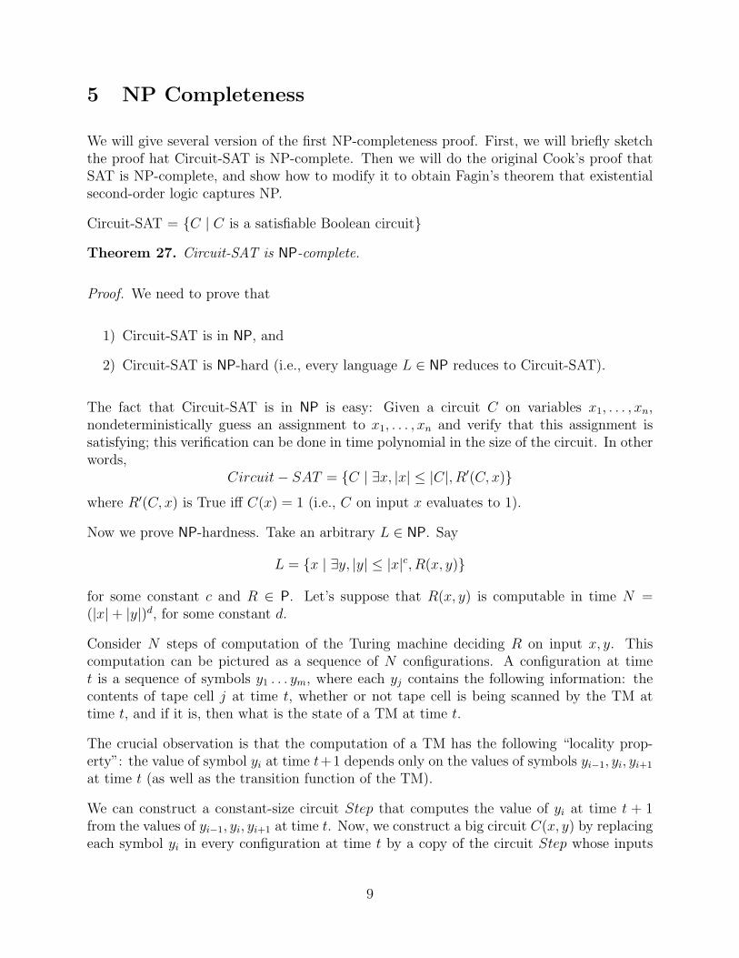
5 NP Completeness

We will give several version of the first NP-completeness proof. First, we will briefly sketchthe proof hat Circuit-SAT is NP-complete. Then we will do the original Cook’s proof thatSAT is NP-complete, and show how to modify it to obtain Fagin’s theorem that existentialsecond-order logic captures NP.

Circuit-SAT = {C | C is a satisfiable Boolean circuit}

Theorem 27. Circuit-SAT is NP-complete.

Proof. We need to prove that

1) Circuit-SAT is in NP, and

2) Circuit-SAT is NP-hard (i.e., every language L ∈ NP reduces to Circuit-SAT).

The fact that Circuit-SAT is in NP is easy: Given a circuit C on variables x1, . . . , xn,nondeterministically guess an assignment to x1, . . . , xn and verify that this assignment issatisfying; this verification can be done in time polynomial in the size of the circuit. In otherwords,

Circuit− SAT = {C | ∃x, |x| ≤ |C|, R′(C, x)}

where R′(C, x) is True iff C(x) = 1 (i.e., C on input x evaluates to 1).

Now we prove NP-hardness. Take an arbitrary L ∈ NP. Say

L = {x | ∃y, |y| ≤ |x|c, R(x, y)}

for some constant c and R ∈ P. Let’s suppose that R(x, y) is computable in time N =(|x|+ |y|)d, for some constant d.

Consider N steps of computation of the Turing machine deciding R on input x, y. Thiscomputation can be pictured as a sequence of N configurations. A configuration at timet is a sequence of symbols y1 . . . ym, where each yj contains the following information: thecontents of tape cell j at time t, whether or not tape cell is being scanned by the TM attime t, and if it is, then what is the state of a TM at time t.

The crucial observation is that the computation of a TM has the following “locality prop-erty”: the value of symbol yi at time t+1 depends only on the values of symbols yi−1, yi, yi+1

at time t (as well as the transition function of the TM).

We can construct a constant-size circuit Step that computes the value of yi at time t + 1from the values of yi−1, yi, yi+1 at time t. Now, we construct a big circuit C(x, y) by replacingeach symbol yi in every configuration at time t by a copy of the circuit Step whose inputs

9

are the outputs of the corresponding three copies of Step from the previous configuration.We also modify the circuit so that it outputs 1 on x, y iff the last configuration is accepting.

The size of the constructed circuit will be at most N ∗N ∗ |Step| (N configurations, at mostN copies of Step in each), which is polynomial in |x|.

Our reduction from L to Circuit-SAT is the following: Given x, construct the circuit Cx(y) =C(x, y) as explained above (with x hardwired into C). It is easy to verify that x ∈ L iffthere is y such that Cx(y) = 1. So this is a correct reduction.

Theorem 28 (Cook-Levin). SAT is NP-complete.

Proof. One way to prove it would be show Circuit− SAT ≤p SAT . But instead we will gothrough the proof as it was originally done, without any references to circuits.

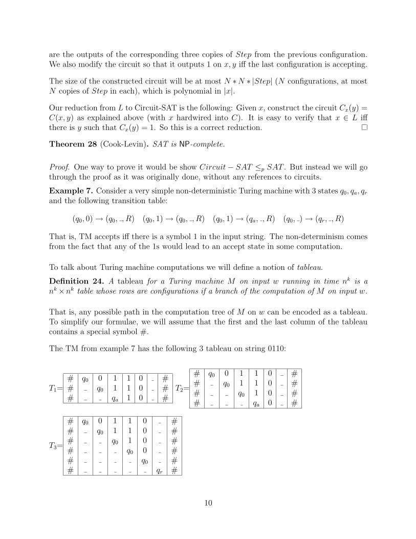
Example 7. Consider a very simple non-deterministic Turing machine with 3 states q0, qa, qrand the following transition table:

(q0, 0)→ (q0, , R) (q0, 1)→ (q0, , R) (q0, 1)→ (qa, , R) (q0, )→ (qr, , R)

That is, TM accepts iff there is a symbol 1 in the input string. The non-determinism comesfrom the fact that any of the 1s would lead to an accept state in some computation.

To talk about Turing machine computations we will define a notion of tableau.

Definition 24. A tableau for a Turing machine M on input w running in time nk is ank×nk table whose rows are configurations if a branch of the computation of M on input w.

That is, any possible path in the computation tree of M on w can be encoded as a tableau.To simplify our formulae, we will assume that the first and the last column of the tableaucontains a special symbol #.

The TM from example 7 has the following 3 tableau on string 0110:

T1=# q0 0 1 1 0 ## q0 1 1 0 ## qa 1 0 #

T2=

# q0 0 1 1 0 ## q0 1 1 0 ## q0 1 0 ## qa 0 #

T3=

# q0 0 1 1 0 ## q0 1 1 0 ## q0 1 0 ## q0 0 ## q0 ## qr #

10

The first two correspond to the accepting branches, the last one to the rejecting. So a NTMaccepts a string iff it has an accepting tableau on that string.

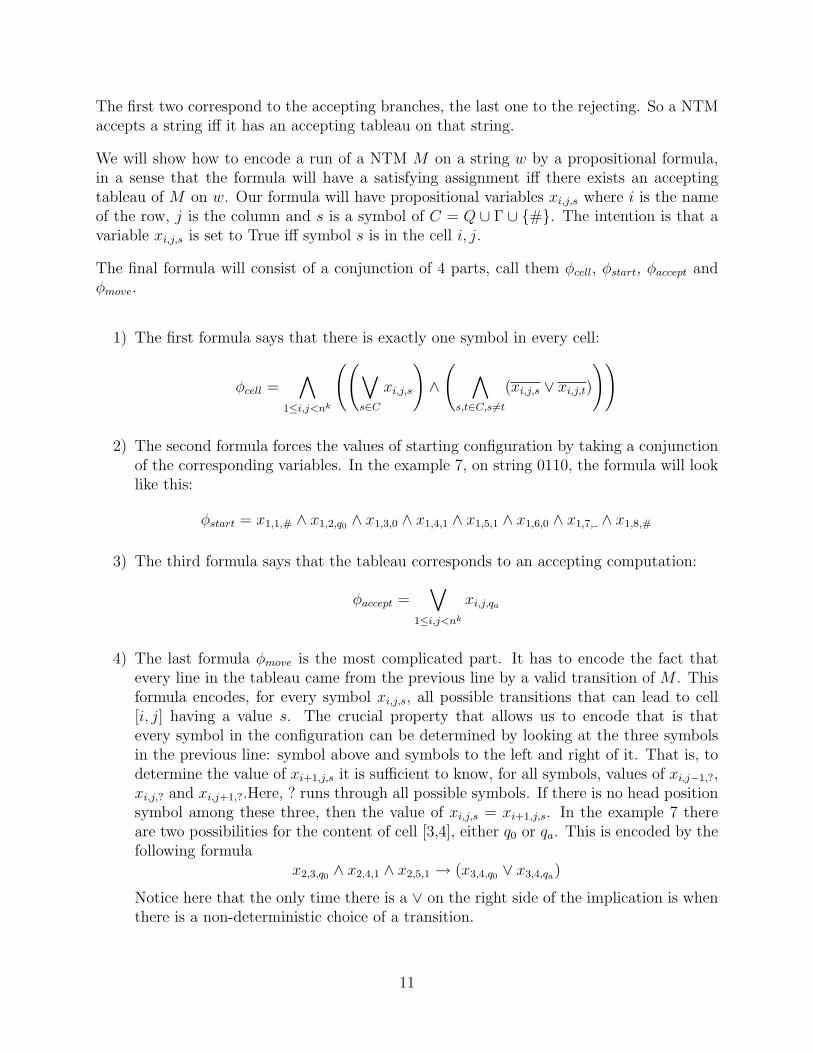
We will show how to encode a run of a NTM M on a string w by a propositional formula,in a sense that the formula will have a satisfying assignment iff there exists an acceptingtableau of M on w. Our formula will have propositional variables xi,j,s where i is the nameof the row, j is the column and s is a symbol of C = Q ∪ Γ ∪ {#}. The intention is that avariable xi,j,s is set to True iff symbol s is in the cell i, j.

The final formula will consist of a conjunction of 4 parts, call them φcell, φstart, φaccept andφmove.

1) The first formula says that there is exactly one symbol in every cell:

φcell =∧

1≤i,j<nk

((∨s∈C

xi,j,s

)∧

( ∧s,t∈C,s6=t

(xi,j,s ∨ xi,j,t)

))

2) The second formula forces the values of starting configuration by taking a conjunctionof the corresponding variables. In the example 7, on string 0110, the formula will looklike this:

φstart = x1,1,# ∧ x1,2,q0 ∧ x1,3,0 ∧ x1,4,1 ∧ x1,5,1 ∧ x1,6,0 ∧ x1,7, ∧ x1,8,#

3) The third formula says that the tableau corresponds to an accepting computation:

φaccept =∨

1≤i,j<nk

xi,j,qa

4) The last formula φmove is the most complicated part. It has to encode the fact thatevery line in the tableau came from the previous line by a valid transition of M . Thisformula encodes, for every symbol xi,j,s, all possible transitions that can lead to cell[i, j] having a value s. The crucial property that allows us to encode that is thatevery symbol in the configuration can be determined by looking at the three symbolsin the previous line: symbol above and symbols to the left and right of it. That is, todetermine the value of xi+1,j,s it is sufficient to know, for all symbols, values of xi,j−1,?,xi,j,? and xi,j+1,?.Here, ? runs through all possible symbols. If there is no head positionsymbol among these three, then the value of xi,j,s = xi+1,j,s. In the example 7 thereare two possibilities for the content of cell [3,4], either q0 or qa. This is encoded by thefollowing formula

x2,3,q0 ∧ x2,4,1 ∧ x2,5,1 → (x3,4,q0 ∨ x3,4,qa)

Notice here that the only time there is a ∨ on the right side of the implication is whenthere is a non-deterministic choice of a transition.

11

Now, suppose that the formula has a satisfying assignment. That assignment encodes pre-cisely a tableau of an accepting computation of M . For the other direction, take an acceptingcomputation of M and set exactly those xi,j,s corresponding to the symbols in the acceptingtableau.

Finally, to show that our reduction is polynomial, we will show that the resulting formulais of polynomial size. The number of variables is N = nk × nk × |Q ∪ Γ ∪ {#}|. In φcellthere are O(N) variables, same for φaccept. Only nk variables are in φstart. Finally, φmove hasO(N × |δ|) clauses. Therefore, the size of the formula is polynomial.

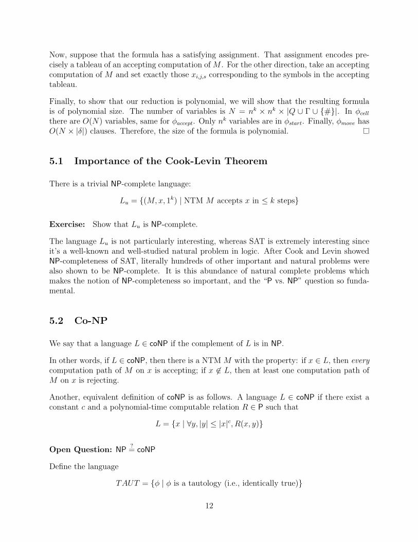
5.1 Importance of the Cook-Levin Theorem

There is a trivial NP-complete language:

Lu = {(M,x, 1k) | NTM M accepts x in ≤ k steps}

Exercise: Show that Lu is NP-complete.

The language Lu is not particularly interesting, whereas SAT is extremely interesting sinceit’s a well-known and well-studied natural problem in logic. After Cook and Levin showedNP-completeness of SAT, literally hundreds of other important and natural problems werealso shown to be NP-complete. It is this abundance of natural complete problems whichmakes the notion of NP-completeness so important, and the “P vs. NP” question so funda-mental.

5.2 Co-NP

We say that a language L ∈ coNP if the complement of L is in NP.

In other words, if L ∈ coNP, then there is a NTM M with the property: if x ∈ L, then everycomputation path of M on x is accepting; if x 6∈ L, then at least one computation path ofM on x is rejecting.

Another, equivalent definition of coNP is as follows. A language L ∈ coNP if there exist aconstant c and a polynomial-time computable relation R ∈ P such that

L = {x | ∀y, |y| ≤ |x|c, R(x, y)}

Open Question: NP?= coNP

Define the language

TAUT = {φ | φ is a tautology (i.e., identically true)}

12

Theorem 29. TAUT is coNP-complete.

Proof. The proof is easy once you realize that TAUT is essentially the same as the comple-ment of SAT. Since SAT is NP-complete, its complement is coNP-complete. (Check this!)

The “NP vs. coNP” question is about the existence of short proofs that a given formula is atautology.

The common belief is that NP 6= coNP, but it is believed less strongly than that P 6= NP.

Lemma 30. If P = NP, then NP = coNP.

Proof. First observe that P = coP (check it!) Now we have NP = P implies coNP = coP.We know that coP = P, and that P = NP. Putting all this together yields coNP = NP.

The contrapositive of this lemma says that: NP 6= coNP implies P 6= NP.

Thus, to prove P 6= NP, it is enough to prove that NP 6= coNP. This means that resolvingthe “NP vs. coNP” question is probably even harder than resolving the “P vs. NP” question.

6 Some NP-complete problems

Recall that proving NP -completeness of a language L by reduction consists of the followingsteps.

1) Show that the language A is in NP

2) Show that A is NP-hard, via the following steps:

(a) Choose an NP-complete B language from which the reduction will go, that is,B ≤p A.

(b) Describe the reduction function f

(c) Argue that if an instance x was in B, then f(x) ∈ A.

(d) Argue that if f(x) ∈ A then x ∈ B.

(e) Briefly explain why is f computable in polytime.

Usually the bulk of the proof is 2a, we often skip 1 and 6 when they are trivial. But makesure you convince yourself they are! Without step 1, your are only proving NP-hardness;with hard enough f you can prove that anything reduces to anything.

13

6.1 Clique-related problems.

We talked before about Clique and IndependentSet problems and showed that Indepen-dentSet reduces to Clique. Now, if we show that IndSet is NP-complete then by transitivityof ≤p and the fact that Clique ∈ NP we get that Clique is NP-complete as well.

Lemma 31. 3SAT ≤p IS.

Givenφ = (x ∨ y ∨ ¬z) ∧ (¬x ∨ w ∨ z) ∧ . . . ()

with m clauses, produce the graph Gφ that contains a triangle for each clause, with verticesof the triangle labeled by the literals of the clause. Plus, add an edge between any twocomplementary literals from different triangles. Finally, set k = m.

In our example, we have triangles on x, y,¬z and on ¬x,w, z, plus the edges (x,¬x) and(¬z, z) (see Figure 6.1).

It remains to be shown that φ is satisfiable iff Gφ has an independent set of size at least k.

Proof. We need to prove two directions. First, if φ is satisfiable, then Gφ has an independentset of size at least k. Secondly, if Gφ has an independent set of size at least k, then φ issatisfiable. (Note that the latter is the contrapositive of the implication “if φ is not satisfiable,then Gφ does not have an independent set of size at least k”.)

For the first (easy) direction, consider a satisfying assignment for φ. Take one true literalfrom every clause, and put the corresponding graph vertex into a set S. Observe that S isan independent set of size k (where k is the number of clauses in φ).

For the other direction, take an independent set S of size k in Gφ. Observe that S containsexactly one vertex from each triangle (clause), and that S does not contain any conflictingpair of literals x and x (since any such pair of conflicting literals are connected by an edgein Gφ). Hence, we can assign the value True to all these literals in the set S, and therebysatisfy the formula φ.

Note that in the proof above, we say things like “take a satisfying assignment to φ” or “takean independent set of Gφ”. These are not efficient steps! But, we don’t need them to beefficient, as they are done only as part of the analysis of the reduction (i.e., the proof ofcorrectness of our reduction), and they are not part of the reduction itself. So the pointis that the reduction must be efficient, whereas the analysis of correctness of the reductionmay involve inefficient (or even non-computable) steps.

Example 8. Consider the following problem: on a network, we want to put monitoringdevices on the nodes of the network so that for every link in the network there is a monitoringdevice on at least one end. The problem of finding a minimal set of vertices enough to cover all

14

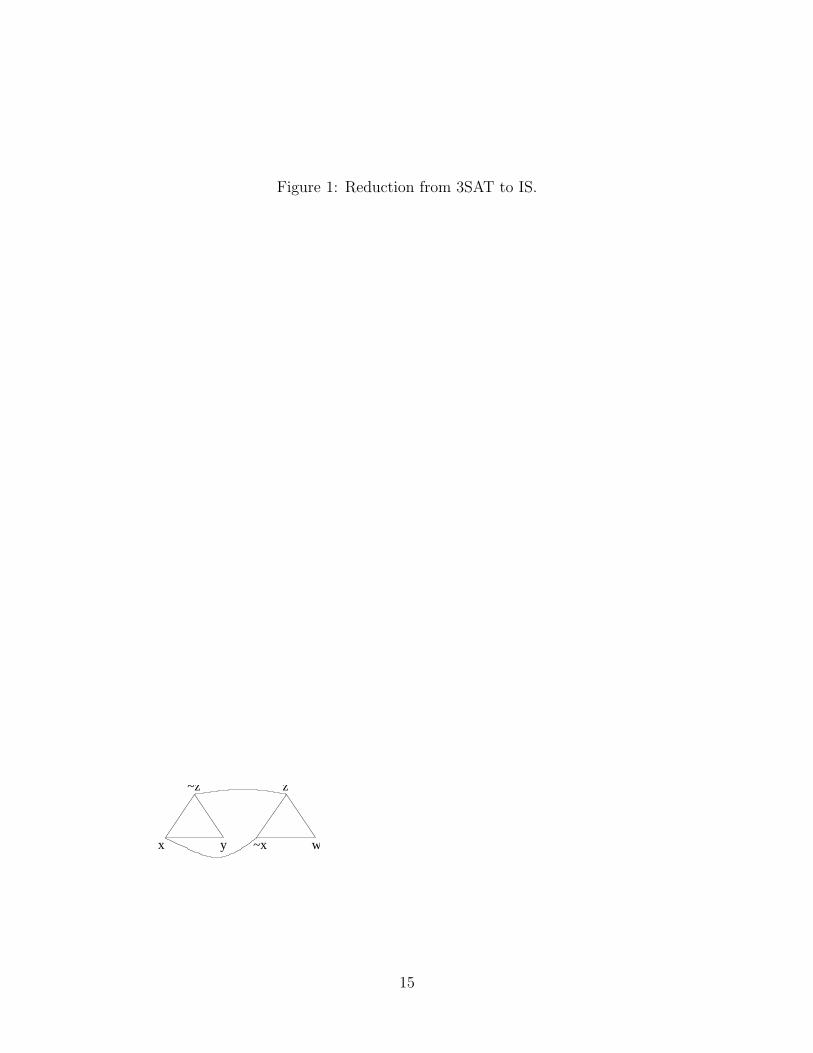
Figure 1: Reduction from 3SAT to IS.

x y

~z

~x w

z

15

vertices is called the Minimal Vertex Cover problem. We are interested in the correspondingNP language: similarly to defining GKD from Knapsack, we define the language V C asfollows.

V C = {〈G, k〉 | ∃S ⊆ V, |S| ≤ k and ∀{u, v} ∈ E, u 6= v, either u ∈ S or v ∈ S}.

Notice that V C ∈ NP: given S, it takes O(|E| ∗ |S|) time to check that every edge in Ghas at least one end in S. To show hardness, we will show that IndSet ≤p V C. We definef(〈G, k〉) = 〈G′, k′〉 by G′ = G and k′ = n − k. Now, we need to argue that the reductionworks. Let S be a largest independent set (can be several of the same size). Then we willshow that V − S is the smallest vertex cover. First, why is V-S a vertex cover? Suppose itis not; then there is an edge both endpoints of which are in S. But this is impossible, sincetwo endpoints the same edge cannot be in an independent set together. Now, why would itbe the smallest vertex cover? Suppose it is possible to throw out of V − S some vertex vand still keep the property that V − S is a vertex cover. This means that the vertex v hasall of its neighbours in V − S. But then there is no reason why it shouldn’t be in S, since ithas no neighbours in there. That would contradict the maximality of S as an independentset. For the other direction we can similarly argue that if V − S is a vertex cover, then Smust be an independent set, and if V − S is minimal, then S must be maximal.

6.2 Satisfiability problems

We already showed that SAT and 3SAT are NP-complete. Another NP-complete variant ofSAT is Not-all-equal SAT, where the acceptance requirement is that an assignment not onlysatisfies at least one literal per clause, but also falsifies at least one literal per clause (in eachclause, not all literals are the same: hence the name).

However, not all variants of SAT are necessarily NP-complete. Consider the following 3variants:

1) 2SAT, where there are at most 2 variables per clause.

2) HornSat, where every clause contains at most one true literal (equivalently, it is of thesame form as Prolog language rules: l1 ← l2 . . . lk).

3) XOR-SAT and XOR-2SAT, where instead of ∨ there is an exclusive OR operation.

All of the following classes are solvable in polynomial time, by different algorithms. Forexample, XOR-SAT can be represented as a system of linear equations over 0,1 and solvedusing Gaussian Elimination. There is a beautiful theorem due to Schaefer (“Schaefer Di-chotomy Theorem”) that states that those are pretty much the only possible subclasses ofSAT, defining by putting a restriction on how a clause might look like, and there is nothingin between. In particular, for SAT over Boolean variables there is no class of formulas with

16

complexity between P and NP, although in general such problem exists, provided P 6= NP.Things get interesting, though, if instead of having Boolean variables you allow more than 2values for the x’s (think fuzzy logic or databases). The case of formulas over 3-value variableshave been solved in 2002 by Bulatov, how have showed, with a lot of work and a help of acomputer, that indeed there is a dichotomy in that case as well. For the 4-valued variablesand higher, the problem is wide open.

6.3 Hamiltonicity problems

Consider two very similar problems. One of them is asking, given a graph, if there is apath through the graph that passes every edge exactly once. Another asks if there is a paththat visits every vertex exactly once. Although these problems seem very similar, in facttheir complexity is believed to be vastly different. The first problem is the famous Euler’sproblem (the “bridges of Koninsberg” problem): the answer is that there is a cycle througha graph visiting every edge exactly once iff every vertex has an even degree; if exactly twovertices have odd degrees then there is a path, but not a cycle. The second problem, calledHamiltonian Path problem, is NP-complete.

Definition 25. A Hamiltonian cycle (path, s-t path) is a simple cycle (path, path fromvertex s to vertex t) in an undirected graph which touches all vertices in the graph. The lan-guages HamCycle, HamPath and stHamPath are sets of graphs which have the correspondingproperty (e.g., a Hamiltonian cycle).

We omit the proof that HamPath is NP-complete (see Sipser’s book page 286). Instead, wewill do a much simpler reduction. Assuming that we know that HamCycle is NP-complete,we will prove that stHamPath is NP-complete. It is easy to see that all problems in this classare in NP: given a sequence of n vertices one can verify in polynomial time that no vertexrepeats in the sequence and there is an edge between every pair of subsequent vertices.

Example 9. HamCycle ≤p stHamPath

Proof. Let f(G) = (G′, s, t) be the reduction function. Define it as follows. Choose anarbitrary vertex of G (say, labeled v). Suppose that there is no vertex in G called v′. Now,set vertices of G′ to be V ′ = V ∪ {v′}, and edges of G′ to be E ′ = E ∪ {(u, v′) | (u, v) ∈ E}.That is, the new vertex v′ is a “copy” of v in a sense that it is connected to exactly the samevertices as v. Then, set s = v and t = v′.

Now, suppose that there is a Hamiltonian cycle in G. Without loss of generality, suppose thatit starts with v, so it is v = v1, v2, . . . vn, v. Here, it would be more correct to use numberingof the form vi1 . . . vin , but for simplicity we assume that the vertices are renumbered. Now,replacing the final v with v′ we get a Hamiltonian path from s = v to t = v′ in G′.

For the other direction, suppose that G′ has a Hamiltonian path starting from s and endingin t. Then since s and t correspond to the same vertex in G, this path will be a Hamiltoniancycle in G.

17

Lastly, since f does no computation and only adds 1 vertex and at most n edges the reductionis polynomial-time.

Note that this reduction would not work if we were reducing to HamPath rather than stHam-Path. Then the part 1c of the proof would break: it might be possible to have a Hamiltonianpath in G′ but not a ham. cycle in G if we allow v and v′ to be in different parts of the path.

Example 10 (Travelling salesperson problem). In the Traveling Salesperson Problem (TSP)the “story” is about a traveling salesperson who wants to visit n cities. For every pair ofthe cities there is a direct connection; however, those connections have very different costs(think flights between cities and their costs). In the optimization problem, the salespersonwants to visit all cities and come back as cheaply as possible; in the decision version, it is aquestion of whether it is possible to visit all cities given a fixed budget B which should coverall the costs.

To model TSP, consider an undirected graph in which all possible edges {u, v} (for u 6= v)are present, and for which we have a nonnegative integer valued cost function c on the edges.A tour is a simple cycle containing all the vertices (exactly once) – that is, a Hamiltoniancycle – and the cost of the tour is the sum of the costs of the edges in the cycle.

TSPInstance:〈G, c,B〉 where G is an undirected graph with all edges present , c is a nonnegative integercost function on the edges of G, and B is a nonnegative integer.Acceptance Condition:Accept if G has a tour of cost ≤ B.

Theorem 32. TSP is NP-Complete.

Proof. It is easy to see that TSP ∈ NP.We will show that HamCycle ≤p TSP.Let α be an input for HamCycle, and as above assume that α is an instance of HamCycle,α = 〈G〉, G = (V,E). Letf(α) = 〈G′, c, 0〉 where:G′ = (V,E ′) where E ′ consists of all possible edges {u, v};for each edge e ∈ E ′, c(e) = 0 if e ∈ E, and c(e) = 1 if e /∈ E.

It is easy to see that G has a Hamiltonian cycle ⇔ G′ has a tour of cost ≤ 0.

Note that the above proof implies that TSP is NP-complete, even if we restrict the edgecosts to be in {0, 1}.

18

6.4 SubsetSum, Partition and Knapsack

SubsetSumInstance:〈a1, a2, · · · , am, t〉 where t and all the ai are nonnegative integers presented in binary.Acceptance Condition:Accept if there is an S ⊆ {1, · · · ,m} such that

∑i∈S ai = t.

We will postpone the proof that SubsetSum is NP-complete until the next lecture. For now,we will give a simpler reduction from SubsetSum to a related problem Partition.

PARTITIONInstance:〈a1, a2, · · · , am〉 where all the ai are nonnegative integers presented in binary.Acceptance Condition:Accept if there is an S ⊆ {1, · · · ,m} such that

∑i∈S ai =

∑j /∈S aj.

Lemma 33. PARTITION is NP-Complete.

Proof. It is easy to see that PARTITION ∈ NP.We will prove SubsetSum ≤p PARTITION. Let x be an input for SubsetSum. Assumethat x is an Instance of SubsetSum, otherwise we can just let f(x) be some string notin PARTITION. So x = 〈a1, a2, · · · , am, t〉 where t and all the ai are nonnegative integerspresented in binary. Let a =

∑1≤i≤m ai.

Case 1: 2t ≥ a.Let f(x) = 〈a1, a2, · · · , am, am+1〉 where am+1 = 2t − a. It is clear that f is computable inpolynomial time. We wish to show thatx ∈ SubsetSum ⇔ f(x) ∈ PARTITION.

To prove ⇒, say that x ∈ SubsetSum. Let S ⊆ {1, · · · ,m} such that∑

i∈S ai = t. LettingT = {1, · · · ,m} − S, we have

∑j∈T ai = a − t. Letting T ′ = {1, · · · ,m + 1} − S, we have∑

j∈T ′ ai = (a− t) + am+1 = (a− t) + (2t− a) = t =∑

i∈S ai. So f(x) ∈ PARTITION.

To prove ⇐, say that f(x) ∈ PARTITION. So there exists S ⊆ {1, · · · ,m + 1} such thatletting T = {1, · · · ,m+ 1}−S, we have

∑i∈S ai =

∑j∈T aj = [a+ (2t− a)]/2 = t. Without

loss of generality, assume m+ 1 ∈ T . So we have S ⊆ {1, · · · ,m} and∑

i∈S ai = t, sox ∈ SubsetSum.

Case 2: 2t ≤ a. You can check that adding am+1 = a− 2t works.

Warning: Students often make the following serious mistake when trying to prove thatL1 ≤p L2. When given a string x, we are supposed to show how to construct (in polynomialtime) a string f(x) such that x ∈ L1 if and only if f(x) ∈ L2. We are supposed to constructf(x) without knowing whether or not x ∈ L1; indeed, this is the whole point. However, often

19

students assume that x ∈ L1, and even assume that we are given a certificate showing thatx ∈ L1; this is completely missing the point.

Theorem 34. SubsetSum is NP-complete

Proof. We already have seen that SubsetSum is in NP (guess S, check that the sum is equalto t). Now we will show that SubsetSum is NP-complete by reducing a known NP-completeproblem 3SAT ≤p SubsetSum.

Given a 3cnf on n variables and m clauses, we define the following matrix of decimal digits.The rows are labeled by literals (i.e., x and x for each variable x), the first n columns arelabeled by variables, and another m columns by clauses.

For each of the first n columns, say the one labeled by x, we put 1’s in the two rows labeledby x and x. For each of the last m columns, say the one corresponding to the clause {x, y, z},we put 1’s in the three rows corresponding to the literals occurring in that clause, i.e., rowsx, y, and z. We also add 2m new rows to our table, and for each clause put two 1’s in thecorresponding column so that each new row has exactly one 1. Finally, we create the lastrow to contain 1’s in the first n columns and 3 in the last m columns.

The 2n + 2m rows of the constructed table are interpreted as decimal representations ofk = 2n + 2m numbers a1, . . . , ak, and the last row as the decimal representation of thenumber T . The output of the reduction is a1, . . . , ak, T .

Now we prove the correctness of the described reduction. Suppose we start with a satisfyingassignment to the formula. We specify the subset S as follows: For every literal assigned thevalue True (by the given satisfying assignment), put into S the corresponding row. That is,if xi is set to True, add to S the number corresponding to the row labeled with xi; otherwise,put into S the number corresponding to the row labeled with xi. Next, for every clause,if that clause has 3 satisfied literals (under our satisfying assignment), don’t put anythingin S. If the clause has 1 or 2 satisfied literals, then add to S 2 or 1 of the dummy rowscorresponding to that clause. It is easy to check that the described subset S is such that thesum of the numbers yields exactly the target T .

For the other direction, suppose we have a subset S that makes the subset sum equal to T .Since the first n digits in T are 1, we conclude that the subset S contains exactly one of thetwo rows corresponding to variable xi, for each i = 1, . . . , n. We make a truth assignmentby setting to True those xi which were picked by S, and to False those xi such that the rowxi was picked by S. We need to argue that this assignment is satisfying. For every clause,the corresponding digit in T is 3. Even if S contains 1 or 2 dummy rows corresponding tothat clause, S must contain at least one row corresponding to the variables, thereby ensuringthat the clause has at least one true literal.

Corollary 35. Partition is NP-complete

Proof. In the last lecture we have showed that SubsetSum ≤p Partition. Since SubsetSumis NP-complete, so is Partition.

20

7 “Search-to-Decision” Reductions

Suppose that P = NP. That would mean that all NP languages can be decided in deter-ministic polytime. For example, given a graph, we could decide in deterministic polytimewhether that graph is 3-colorable. But could we find an actual 3-coloring? It turns out thatyes, we can. In general, we can define an NP search problem: Given a polytime relation R,a constant c, and a string x, find a string y, |y| ≤ |x|c, such that R(x, y) is true, if such ay exists. We already saw (recall theorem 25 on page 5) that if P = NP, then it is possibleto compute the certificate in polynomial time. Now we will expand on this, showing howthe ability to get access to the answer to the decision problem allows us to solve the searchproblem.

This is not as trivial matter as it seems from the simplicity of the reductions. This methodproduces some certificate of the membership, not necessarily one you might like to know.As a prime (pun intended) example, remember that testing whether a number is prime canbe done in polynomial time; however, computing a factorization of a composite number isbelieved to be hard, and is a basis for some cryptographic schemes (think RSA).

Theorem 36. If there is a way to check, for any formula φ, if φ is satisfiable, then thereis a polynomial-time (not counting the check) algorithm that, given a formula φ(y1, . . . , yn),finds a satisfying assignment to φ, if such an assignment exists.

Proof. We use a kind of binary search to look for a satisfying assignment to φ. First, wecheck if φ(x1, . . . , xn) ∈ SAT . Then we check if φ(0, x2, . . . , xn) ∈ SAT , i.e., if φ with x1 setto False is still satisfiable. If it is, then we set a1 to be 0; otherwise, we make a1 = 1. Inthe next step, we check if φ(a1, 0, x3, . . . , xn) ∈ SAT . If it is, we set a2 = 0; otherwise, weset a2 = 1. We continue this way for n steps. By the end, we have a complete assignmenta1, . . . , an to variables x1, . . . , xn, and by construction, this assignment must be satisfying.

The amount of time our algorithm takes is polynomial in the size of φ: we have n steps,where at each step we must answer a SAT question. Since we did not count the time toanswer a SAT question in our computation time, the rest of each step takes polytime.

One way of thinking about this type of problem is that if P = NP, then a certificate to anyx ∈ L for any L ∈ NP can be computed in polynomial time. Another way is to imagine agiant precomputed database somewhere in the cloud storing answers to, say, all instances ofSAT up to a certain (large enough) size. Suppose that our algorithm can send queries tothis database and get back the answers. Since these answers are already precomputed, thereis no time (and at least no our time) spent retrieving them. Of course, this dataset wouldbe enormous.

As another example of the search-to-decision reduction, consider the Clique search problem.Assuming that there is a procedure CliqueD(G, k) which given a graph G and a number ksays “yes” if G has a clique of size k and “no” otherwise, design an algorithm CliqueS(G)

21

finding a clique of maximum size as follows. First, ask CliqueD(G, n). If the answer is “yes”,then G is a complete graph and we are done. If not, proceed doing a binary search on k todetermine the size of the largest clique (it does not quite matter in this problem whetherit is a binary search or a linear search, but it does matter for other applications). Supposekmax is the size of the maximum clique. Now, find an actual clique by repeatedly throwingout vertices and checking if there is still a clique of size kmax in the remaining graph; if not,you know that the vertex just thrown out was a part of the clique and should be kept in Gfor the following iterations.

It should be stressed that we are interested in efficient (i.e., polytime) search-to-decisionreductions. Such efficient reductions allow us to say that if the decision version of ourproblem is in P, then there is also a polytime algorithm solving the corresponding searchversion of the problem.

22