Complex Network Analysis of Men Single ATPTennis Matches

Umberto MichieliDepartment of Information Engineering, University of Padova – Via Gradenigo, 6/b, 35131 Padova, Italy

michieli@dei.unipd.it

Abstract—Who are the most significant players in the history ofmen tennis? Is the official ATP ranking system fair in evaluatingplayers scores? Which players deserved the most contemplationlooking at their match records? Which players have never facedyet and are likely to play against in the future? Those are justsome of the questions developed in this paper supported by dataupdated at April 20181.In order to give an answer to the aforementioned questions,complex network science techniques have been applied to somerepresentations of the network of men singles tennis matches.Additionally, a new predictive algorithm is proposed in order toforecast the winner of a match.

Index Terms—Tennis, Complex Network, Ranking, Link Pre-diction, Community Dectection.

I. INTRODUCTION AND RELATED WORKS

During the last decades Network Science field has beenrediscovered and addressed as the "new science" [2], [3]. A lotof issues have been (re-)examined thanks to Network Sciencetechniques, which are nowadays permeating the way we facethe world as a unique interconnected component. The presenceand the immediate availability of a huge amount of digital datadescribing every kind of network and the way in which itsnodes interact, has made possible an interdisciplinary analysisof many large-scale systems.Similar techniques have been recently applied also to pro-fessional sports, in order to discover complex interactionsphenomena and universal rules which are almost invisibleand difficult to recognize restricting the attention to smallnetworks or to microscopic level. For example, complex-network analysis were conducted on soccer (e.g. in [4] and[5]), football ([6] and [7]), basket ([8] and [9]), baseball ([10])and cricket ([11] and [12]), just to name a few.

In professional tennis as well, there are few studies ex-amining how to map matches into complex networks andthen developing new ranking methods alternative to the ATP(Association of Tennis Professionals) official one.The first work of this kind is represented by [13], wherethe authors explained the network generation and then theyperformed some simple analysis on single Grand Slamstournaments matches only (i.e. four tournaments each year:respectively Australian Open, Roland Garros, Wimbledon andU.S. Open). Then an important contribution was brought by[14], where a different network modeling is proposed and the

1The datasets used in this paper are made publiclyavailable at: https://drive.google.com/open?id=1mCxZfkkpIC9o-nxZ1yW3GBBdvBOPW6mQ [1]

PageRank algorithm is applied identifying Jimmy Connors asthe most important single tennis player between 1968 and2010.More recent tennis-related complex network studies regardnew ranking methods proposal and evaluations (see as ref-erence [15], [16] and [17]), or are related to doubles matches[18] or to the gender and handedness effects in top rankingpositions [19].

On the other side, however, in literature there is not anexhaustive and precise explanation about the network topologyof the tennis matches graph. Moreover, some papers seemsto be hasty in asserting a scale-free nature of the networkwith some inaccuracies. In this study the resulting networkstructure when all the official men single tennis matchesare considered since the so-called "Open Era" to the end ofMarch 2018 (i.e. from 1968 onward; the ATP organization,instead, was founded in 1972) is carefully analyzed and all itsmajor properties are stated, which can be exploited for someinteresting structural considerations, even not touched in theexisting studies, and for further analysis.

In the second part of the paper some ranking algorithmshave been applied aiming at confirming the present literatureon ranking methods, thus seeing how active tennis players haveimproved their overall prestige over the recent years. However,at the same time, the aim of the paper is to provide someuseful considerations about link prediction and communitiesdetection.All the computer simulations were performed in Matlab.

II. GENERATION OF DATASET AND NETWORK

The first step is the generation of the dataset: all men tennismatches since 1968 are considered. The data can be freelydownloaded directly from the ATP website [20] and from otheronline repositories (like [21] for recent data and [22]) allowingto fix some inconsistencies in the official ones. Hence the firststep to do is to merge the small datasets, provided on a yearlybasis, in one only; this is a very delicate operation since weneed to account for many format differences and bring them allback to a common language for the information’s specification.For some of the next considerations the following features ofinterest for each match have been kept: the tournament level,the tournament stage, the winner player and the loser player.A brief excursion follows in order to explain those quantities.The tournament levels allows to identify the importance of amatch, in fact ATP hosts tournaments of very different prizes

arX

iv:1

804.

0813

8v1

[ph

ysic

s.so

c-ph

] 2

2 A

pr 2

018

(as regards both money and ATP ranking points assigned),which in increasing order of importance are: ATP 250 tourna-ments, ATP 500, Masters 1000, the annual ATP World TourFinals and the Grand Slams (different names were used in thepast but similar considerations hold). The ATP points assignedto the winner of the tournament are respectively 250, 500,1000, 1500 and 2000 and lower points are attributed to theplayers in proportion to the reached stage of the tournament(e.g round 128, round 64, up to semifinal and final); refer toTable II for a simplified overview of current points attributiondistribution where points of qualified players are taken intoaccount as last rounds of each entry (more detailed systempoints attribution can be examinated in [23]).

With those considerations in mind it is possible to map thematches into many different network representations (in all ofthem, however, the nodes represent the players, hence theyare homogeneous) and the main scenarios are summarized inFigure 1 matching the following descriptions:

1) Direct graph representation: in this model an edgeexists from every loser to the winner, each link has aweight equal to the number of times the destination nodewon over the starting node. In case of multiple links theweights are just summed. Similar representations wereadopted in [14] considering data up to 2010, in [13] con-sidering data between 90s and 00s of male and femalematches of Grand Slams only with different weightsfunction, and in [15] with data of top-100 players onlyand different weights function. The obtained graph isnot symmetric, not even if the respective unweightedversion is considered.

2) Direct and symmetric graph representation: thisoriginal proposal assumes the existence of a directed linkbetween each couple of nodes which played at least onematch against each other. The weights are the respectiveATP points awarded by the two players; note that eventhe loosing player gets a non-negative points score. Alsoin this representation in case of multiple links the pointsare summed up. By construction, the network will bestructurally symmetric but with possibly very differentweights.

3) Undirect (and unweighted) graph representation: formany considerations, however, the most useful repre-sentation is the one where two players are connectedthrough an undirected and unweighted edge if they playat least one match against each other, thus we obtain anundirected and symmetrical network.

4) Extended version of undirect and unweighted graph:this is the largest possible dataset since official tennismatches have been established because it takes intoaccount also Davis Cup, Challenger and Futures tour-naments since 1991, which were not considered in thefirst three datasets. Two players are connected throughan undirected and unweighted edge if they play at leastone match against each other.

The first three datasets are formed by N = 4245 nodes

1.

w

Loser Winner

w=# of times P1 wins agains P2

2. w,

W2

Loser Winner

w1=sum of the ATP points awarded by P1

in matches against P2

w2=sum of the ATP points awarded by P2

in matches against P1 3.

1

Loser Winner

Figure 1. Three different network representations considered; each edge isassociated to a respective weight briefly explained.

(i.e. players) and a total of 151734 matches which leadsto L = 170168 or 101436 links depending on the selectedrepresentation (larger number for the second representation).The fourth dataset comprises of N = 22405 players andL = 998114 links.

Notice that, as in many real networks, the matrix can still

be defined as sparse since it holds L � Lmax =N(N − 1)

2links, where Lmax is the maximum number of links of anetwork with N nodes.These large datasets will allow us to spot general trends andmost competitive players overall; for more specific analysisit is enough just to restrict the attention to a smaller periodof time (e.g. if we are interested in a specific player weshould consider restricting our focus to his career epoch). Forconstruction, some results can be inherently biased toward thealready retired players but in practice we will see that thisdoes not always hold because of, for example, the increasingnumber of tournaments and of ATP points assigned each year.

III. TOPOLOGICAL RESULTS

In this section some results of complex network techniquesare explored highlighting the properties and the underlyingphysical meaning. Moreover some comparisons among thedifferent network representations will be asserted to verify thecommon aspects through different views.

A. Adjacency Matrix

In Figure 2 the adjacency matrix of the first representationof direct network is shown. The plot of the matrix has this

W F SF QF R16 R32 R64 R128Grand Slam 2000 1200 720 360 180 90 45 10ATP World Tour Finals +500 +400 +200 points for each round robin match winMasters 1000 1000 600 360 180 90 45 25 15ATP 500 500 300 180 90 45 20 10ATP 250 250 150 90 45 20 10 5

Table IATP POINTS DISTRIBUTION. W=WINNER, F=FINALIST, SF=SEMI FINALIST, QF=QUARTER FINALIST, R=ROUND.

Figure 2. Adjacency matrix of the direct network representation.

shape because, by construction, first of all the players whichhave won at least one match are inserted and after that theplayers which figure only for lost matches are considered.Thus, since there can’t be any link between two always-loserplayers, the bottom-right part of the matrix is composed byall-zero entries. The bottom-left part of the matrix (and therespective up-right part if symmetric case is considered) dohave a few points which are the matches lost by players whoonly have lost matches in the higher ATP tournaments (theysurely have won some matches in minor ATP tournaments likeChallengers or Futures in order for them to be admitted in themain draw of the most important ATP tournaments).Moreover notice that the columns and the rows with a lot ofnon-zero entries are associated with players who have faceda lot of different players, thus usually they are players with along-career and very successful, we should come back to thisidea of evaluation of successful player in section III-E and inIII-I.

B. Network Visualization and Small World Property

In Figure 3 the visualization of the small direct network isshown.

Figure 3. Direct network visualization.

By simply looking at the network topology and remember-ing how the network was constructed, we could already imag-ine that a giant component is present and that the small worldproperty holds. By numerical evaluations, indeed, we foundthat in the direct representation there is one giant componentof size 2428 nodes and all the other components are unitary(in the undirect network there is just one component whichcontains all the nodes of the network). Defining the shortestpath between any two nodes as the distance between thosenodes we can derive the average distance of the direct graph

defined as 〈d〉 =1

N

N∑i=1

di with di =1

N

N∑j=1

min(dij) which

lead to 〈d〉 ≈ 3.48 hops (and for the small undirect network is〈d〉 ≈ 3.34 hops, for the large undirect network is 〈d〉 ≈ 3.64hops). Moreover the diameter of the network, i.e. the maxi-mum of all the shortest paths, is diam = max(min(dij)) = 10hops (and diam = 8 hops for the small undirect network,diam = 9 hops for the last network).Hence, the networks exhibit actually a strong small worldproperty which leads to very short distances between anychosen pair of nodes. In order to better visualize it we couldalso look at the plots of the percentage of nodes within aconsidered directed hop distance as in Figure 4 and we realizethat the worst cases are achieved only by a small fraction ofnodes, thus reducing the variance of this metric. Notice thatthe blue curve for the first direct graph does not reach 100%because some of the nodes are disconnected from the giantcomponent.

0 2 4 6 8 10 12

Hop distance

0

10

20

30

40

50

60

70

80

90

100

% o

f pai

rsPercentage of pairs whithin hop distance

DirectUndirect

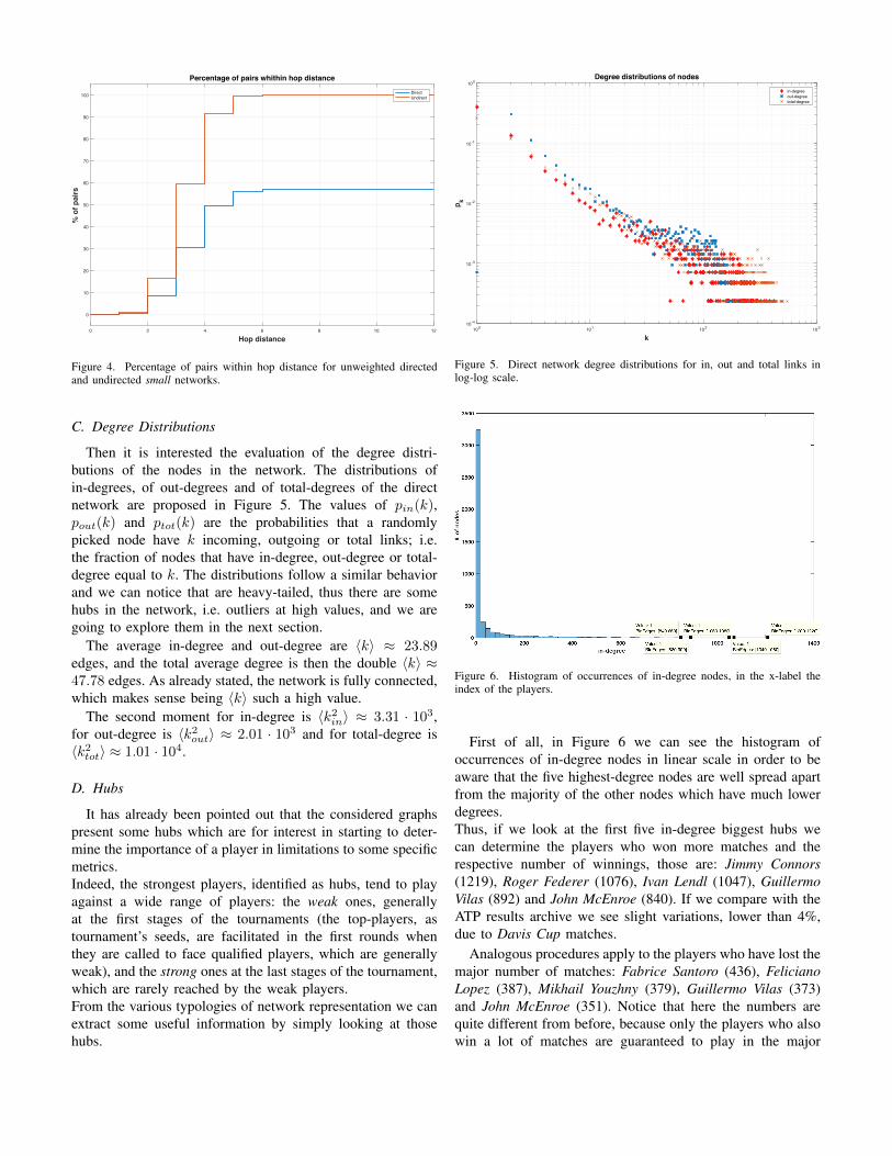
Figure 4. Percentage of pairs within hop distance for unweighted directedand undirected small networks.

C. Degree Distributions

Then it is interested the evaluation of the degree distri-butions of the nodes in the network. The distributions ofin-degrees, of out-degrees and of total-degrees of the directnetwork are proposed in Figure 5. The values of pin(k),pout(k) and ptot(k) are the probabilities that a randomlypicked node have k incoming, outgoing or total links; i.e.the fraction of nodes that have in-degree, out-degree or total-degree equal to k. The distributions follow a similar behaviorand we can notice that are heavy-tailed, thus there are somehubs in the network, i.e. outliers at high values, and we aregoing to explore them in the next section.

The average in-degree and out-degree are 〈k〉 ≈ 23.89edges, and the total average degree is then the double 〈k〉 ≈47.78 edges. As already stated, the network is fully connected,which makes sense being 〈k〉 such a high value.

The second moment for in-degree is 〈k2in〉 ≈ 3.31 · 103,for out-degree is 〈k2out〉 ≈ 2.01 · 103 and for total-degree is〈k2tot〉 ≈ 1.01 · 104.

D. Hubs

It has already been pointed out that the considered graphspresent some hubs which are for interest in starting to deter-mine the importance of a player in limitations to some specificmetrics.Indeed, the strongest players, identified as hubs, tend to playagainst a wide range of players: the weak ones, generallyat the first stages of the tournaments (the top-players, astournament’s seeds, are facilitated in the first rounds whenthey are called to face qualified players, which are generallyweak), and the strong ones at the last stages of the tournament,which are rarely reached by the weak players.From the various typologies of network representation we canextract some useful information by simply looking at thosehubs.

10-4

10-3

10-2

10-1

100

p k

Degree distributions of nodes

100 101 102 103

k

in-degreeout-degreetotal-degree

Figure 5. Direct network degree distributions for in, out and total links inlog-log scale.

Figure 6. Histogram of occurrences of in-degree nodes, in the x-label theindex of the players.

First of all, in Figure 6 we can see the histogram ofoccurrences of in-degree nodes in linear scale in order to beaware that the five highest-degree nodes are well spread apartfrom the majority of the other nodes which have much lowerdegrees.Thus, if we look at the first five in-degree biggest hubs wecan determine the players who won more matches and therespective number of winnings, those are: Jimmy Connors(1219), Roger Federer (1076), Ivan Lendl (1047), GuillermoVilas (892) and John McEnroe (840). If we compare with theATP results archive we see slight variations, lower than 4%,due to Davis Cup matches.

Analogous procedures apply to the players who have lost themajor number of matches: Fabrice Santoro (436), FelicianoLopez (387), Mikhail Youzhny (379), Guillermo Vilas (373)and John McEnroe (351). Notice that here the numbers arequite different from before, because only the players who alsowin a lot of matches are guaranteed to play in the major

tournaments, otherwise after a while you loose the right toplay in.

Surely the results seen up to now tend to promote alreadyretired players and/or with a long career. On the other side,if we think of applying similar techniques for the networkwith ATP ranking weights, we see quite different outcomespromoting current-time players because nowadays there aregreat players, of course, but also more tournaments whichgive even more ATP points than in the previous generations oftennis players. Thus the five players who gained the most ATPpoints are: Roger Federer, Rafa Nadal, Novak Djokovic, JimmyConnors and Ivan Lendl. Unfortunately some inaccuraciesare present in the translation of current ATP points for oldmatches.

Looking at the degree distributions in Figure 5 and at theresults we are suggested to consider an underlying assumption:the more connected athletes are and the most likely is to bebest players. Most of the players have a small number ofmatches and then quit playing the major tournaments, on thecontrary, there is a small group of top-players who performmany matches against weaker players and among themselves.This phenomenon is an observation of the rich get richer effectdriven by the attractiveness of the high connected nodes asopponent for new-comers; an interpretation of the richnessthat the players achieve could be their gain of some sort of"experience" during the matches of their carreer, as alreadypointed out in [13].

E. Considerations on Network Nature

The most critical point in the analysis already presentin literature on this topic is the scale-free nature of suchnetworks. A first-step analysis about the network nature canbe done by plotting again the degree distribution (e.g. thein-degree) and trying to fit it with some typical networkdistributions. The results are shown in Figure 7 where wecan appreciate the differences among them. The respectiveparametric formulations of distributions together with fittingparameters and the coefficient of determination R2 are re-ported in Table II. As already noticeable by the presenceof hubs, the network cannot clearly follow a random model(the poisson one) and some heavy-tailed distributions need tobe considered. The power-law and the Lévy distributions arethe two models performing better on the raw data, thus theconsidered network exhibits many properties typical of scale-free networks.Assuming the network as power-law, we can measure thescale-free parameter γ: it is found to be γin ≈ 1.66 for in-degrees, γout ≈ 2.12 for out-degrees and γundirect ≈ 1.38for the undirect network, values which are consistent with theones found in literature in [14] and [13].

The aforementioned results need to be taken with somecautions; the network characteristics are quite similar to scale-free networks (they are even more similar when we restrictour interest to top-players and/or to top-tournaments only) andscaling behavior is also suggested by the structural preferentialattachment of new players who generally tend to connect to an

existing player with a probability proportional to the degree ofsuch node. However if we try to reduce the noise around theoutliers, e.g. by considering the cumulative degree distributionor a log-binning of the data, we can see that the network is nota pure scale-free model and it would make sense to limit theintervals introducing cutoff values kmin and kmax, as carefullyproved in [24] in a general setting. Moreover, as suggested in[25] we should not rely on the R2 parameter, since it is provedto achieve very high values also for non scale-free networks.Summing up: the fit on raw data based on R2 is source ofmany errors in current literature about network analysis.

Hence, the Complementary Cumulative Distribution Func-tion (CCDF) should be considered and it is plotted in Figure 8;here the issue of the plateau corresponding to values occurringonce has been solved and we can confirm the previousconsiderations since power-law networks would describe astraight line in a log-log plot.More specifically, replicating the fitting on the cumulativedistribution, the network can be categorized as a power-lawwith an exponential cut-off, i.e. pk ∝ x−αe−

kβ : indeed we

can observe in Figure 8 that the curve starts out as a powerlaw and ends up as an exponential.This result confirms that R2 on raw data cannot be trusted andthat, maybe, often is just worth noticing that the distributionhas a heavy tail instead of asserting immediately its scale-freenature, which is a very widespread practice (many interestingconsiderations about networks and fitting techniques can beread in [25]).The fact that the complete network is not scale-free is aquite surprising result, although very clear from the CCDFplot, because all other related studies on tennis network areaffirming the scale-free nature and are deriving from there theinteresting properties of the network, which is not preciselycorrect.Some power-law networks with coefficient lower than 2 ornot scale-free networks at all have gained a lot of attentionin recent literature, for example in [26] and [27], becausethose models have been discovered in many real scenarioswhere the number of new links generally grows faster than thenumber of new nodes, which is precisely our situation. Thenumber of annual tennis matches is nowadays very big andtherefore the probability of a new connection is much morefrequent than the new players who join the most importantATP tour. Thus it may seem that the network should evolvetoward a non-sparse adjacency matrix, which is still not thecase because of structural constraints: is very unlikely thatsome pairs of players will face against each other (because ofplayers’ retirement from the tour or players which are stronglyfar apart in ranking) but on the other hand the hubs role oflong-career players will be even reinforced.

F. Clustering Coefficient

Another interesting property of small world network is theclustering coefficient C. For a node j its clustering coefficient,Cj , is a number belonging to [0, 1] denoting how manylinks there are between its neighboring nodes normalized to

pmf or PDF Numerical parameters R2

Poisson pk = e−λλk

k!λ = 〈k〉

Exponential pk = λe−λk λ = 1 0.9879

Power-law pk ∝ k−γ γ = 1.66 0.998

Log-normal pk =1

xσ√2πe− (ln(x)−µ)2

2σ2 µ = −0.14 σ = 1 0.9938

Weibull pk = abx(b−1)e−a∗xb

a = 0.93 b = 1.06 0.9866

Lévy pk =

√c

2π

e− c

2(x−µ)

(x− µ)3/2µ = 0.39 c = 0.57 0.9979

Table IIFITTING DISTRIBUTION APPLIED TO IN-DEGREE RAW DATA.

10-4

10-3

10-2

10-1

100

p k in

Degree distribution of in-degree and fitting

100 101 102 103

kin

in-degreepoisson <k>=mean( kin )exponential =1power law =1.66log-normal =-0.14 =1Weibull a=0.93 b=1.06Levy =0.39 c=0.57

Figure 7. Fitting trials of raw data of in-degrees, log-log scale.

100 101 102 103

kin

10-4

10-3

10-2

10-1

100

1-P(

k in)

1-CDF of p kin

Figure 8. Complementary Cumulative Distribution Function (CCDF) in log-log plot.

0 0.1 0.2 0.3 0.4 0.5 0.6 0.7 0.8 0.9 1

Clustering Coefficient C

0

0.1

0.2

0.3

0.4

0.5

0.6

0.7

0.8

0.9

1

P(x<

=C)

Clustering coefficient distribution

Figure 9. Clustering coefficient distribution of the undirect representation.

the maximum possible number of links among them; moreformally could be defined as Cj = Ej/Ej,max where Ej isthe number of edges between nodes in the neighborhood of j(Nj) and Ej,max is its maximum value.For example, in undirect networks it holds 0 ≤ Ej ≤Ej,max = |Nj |(|Nj | − 1)/2. Finally, the general clusteringcoefficient is expressed as the average over all the N players:

C =1

N

N∑j=1

Cj .

In the undirect representation of the network we have foundC = 0.07, which is coherent as order of magnitude with thevalues found in [13]; as a term of comparison, in Figure 9 isreported the clustering coefficient distribution, i.e. the fractionof nodes having clustering coefficient lower than c.

G. Degree Correlation

Another interesting metric on the network point of viewis the correlation between the degrees of nodes. Degreecorrelation can be expressed in many ways, usually the Pear-son assortativity coefficient is used as principal investigationmethod and is defined as:

r =

∑max(k)h=min(k)

∑max(k)f=min(k) hf(ehf − qhqf )

σ2

where qh is the probability of finding a degree-h node atthe end of a randomly picked link, ehf is the probabilityof finding a link between two nodes of degree h and f , σ2

is the variance of the degrees and can be proved to be themaximum of the numerator, thus r ∈ [−1, 1]. Computingthis parameter for the small undirect and unweighted networkwe found r = −0.0076 which means a slightly assortativenetwork and actually almost neutral, probably because hubsand small degree nodes are likely to play against in the firststages of the tournaments but also hubs tend to play againstthemselves in the final rounds, thus no strong pattern exists.For the large undirect network r = 0.272 is found.

H. Robustness to Failures

For a more complete characterization of the network struc-ture it could be interested to analyze its robustness to failures,i.e. the nodes removal from the network. In the chosen networka player could be disqualified for doping or other reasons, orwe could need to consider just a subset of players or matches(restricting by nationality, left or right handedness, heightthreshold, tournament level and so on). We want to determinethe robustness of the network in terms of percentage of nodesconnected to the giant component when f% of its nodeshas been removed. In the following we are just consideringrandom removals and attack-based removals since all the otherare mainly application-driven and can be done with a smalleffort manipulating the dataset as desired. In the first scenarioconsidered the nodes are removed entirely at random while inthe second scenario the highest hub in the network is removedat each step. We introduce the probability that a random nodebelongs to the giant component after that f% of nodes havebeen removed as P∞(f) and we can look at the relative size ofthe giant component: P∞(f)/P∞(0), where P∞(0) representsthe best case of no removals thus the ratio belongs to [0, 1].The plot of such ratio for the undirect graph is shown inFigure 10 and we recognize in our network the high robustnesstypical to well-connected and scale-free graphs. The black linecorresponds to 1−f and it is an upper limit since for sure wehave removed f% of nodes from the network (and then alsofrom the giant component).

I. Ranking Methods and Predictive Power

The main interest in analysis of tennis networks is directedtowards the implementation of new ranking techniques in-stead of the ATP ranking system, together with their relativepredictive power when a new match is played. There areno contributions in literature, instead, for what concerns linkprediction (e. g. who are the most probable players to playagainst given that they did not played against before?) andcommunity detection.Radicchi in [14] is the first who applied the PageRank (PR)algorithm to tennis network thus identifying Jimmy Connorsas the most valuable player in the tennis history. Dingleet al. in [23] applied the previous work to ATP and WTA(Women’s Tennis Association) matches and they also provideda simple comparison on the basis of predictive power. In [15]

0 0.1 0.2 0.3 0.4 0.5 0.6 0.7 0.8 0.9 1

f failure rate

0

0.1

0.2

0.3

0.4

0.5

0.6

0.7

0.8

0.9

1

P(f)

/P(0

)

1-fRandom FailuresAttacks

Figure 10. Robustness of the undirect network after f% of nodes removals.

the authors proposed yet another ranking method applyingPageRank to the subgraph of the Top-100 players. In [16]many ranking methods, both through network and Markovchains analysis, have been proposed and verified by meansof prediction power.

Also few other non-network-related approaches have beenproposed so far: for example in [28] statistical models havebeen tested to improve the current ranking system, or in [29]the authors applied a novel method exploiting neural networksbased on 22 features and achieving a 75% benefit in predictionthrough those techniques.

1) Preliminaries on Ranking Algorithms: The analysisshown in this section assumes the direct representation of thenetwork where the loser player has an edge to the winnerplayer and the weight corresponds to the number of matcheswon by the winner.The link analysis methods investigated in this report are: Hubsand Authorities (HITS algorithm, Hyperlink-Induced TopicSearch discussed in [30]), simple PageRank and PageRankwith teleportation (see [31] and [32] as references).

The idea on which HITS algorithm is based regards thedefinitions of hubs and authorities. Authorities are nodes witha high number of edges pointing to them, hubs are nodeswhich link to many authorities; in our scenario, intuitively,we expect that authorities are often associated with the mostsuccessful players (because they won against a wide gammaof players), while the hubs with mediocre players with a longcareer. More formally we can compute the authority-scores aand the hub-scores h respectively as:

a =Ah

||Ah||h =

ATa

||ATa||

where we assumed the adjacency matrix to be the transposedversion of the one presented above (i.e. here an entry aij = 1means that there is a link from node j to node i). Notice thatai ≥ 0 and hi ≥ 0 ∀i. The problem can be solved throughpower iteration with convergence parameter ε.

The rationale behind PageRank is that of a random walkalong the graph and the prestige score p for each playeris determined as the probability of being at that node instationarity conditions. The t-th update of p goes as:

pt = Mpt−1

where M is the column stochastic adjacency matrix.The simple PageRank algorithm is affected by some un-

desirable problems. For example it would end up in deadends, although it is not the case because who win one matchwill surely lose one other (unless the player plays onlytournaments winning all of them, which never happens); andthere also might be periodic behavior looping in cycles, whichis somehow reasonable to expect since we are consideringvery different tennis epochs. Thus we can add to the modelthe possibility of not to follow the behavior but to jump toa random node in the network with a probability α ∈ (0, 1).Hence the t-th update step of p becomes:

pt = M̆pt−1 = (1− α)q11Tpt−1 + αMpt−1

where q1 is the stochastic teleportation vector and we assumedit to be q1 = 1

N 1 (equal probabilities), with 1 column vectorof N ones; α is a damping factor typically set to 0.85 (thisis due to historical reasons as proposed in the original paper[32] and for the sake of comparisons with other works). Thisconsiderations let to write a much simpler iteration procedurethan the one proposed in [14] and [23], although they areequivalent. The simplifications are made possible thanks tothe observation regarding the absence of sinks-like nodes andto a compact vectorial expression.

2) Discussion of results: Hubs and authorities scores arereported in Figure 11, where can be seen that nodes IDcorresponding to players who only have lost matches (the lastones) have zero authority score, because there are no linkspointing to them, but possibly non-zero hub score.The names of the Top-20 hubs and authorities are reportedin the second and third columns of Table III for ε = 10−8;few changes happen varying this parameter and most of themnot in the very first positions. Though there are no referenceliterature of HITS applied to tennis, nevertheless from the tablewe can confirm our previous intuition and also realize thatthose concepts are somehow similar to what already discussedtalking about in-degree and out-degree hubs. Indeed, we canrecognize that in-degree hubs and out-degree hubs are placedin the first positions respectively of authorities and of hubs,although not in the precise order. Compare these results withsection III-D

In terms of complexity we expect at most tmax iterationsfor the HITS algorithm to converge, where:

tmax =

⌈− ln(ε)− ln(

√N)

2 ln(d1/d2)

⌉with d1 and d2 being the eigenvalues associated with the twohighest eigenvectors of M = AAT. Setting ε = 10−8 itresults in tmax = 180 iterations, but in order to converge just

0

0.05

0.1

0.15

0.2

0.25

0.3

Scor

es

HITS hubs and authorities

0 500 1000 1500 2000 2500 3000 3500 4000 4500

nodes ID

HubsAuthorities

Figure 11. Hubs and authorities scores of HITS algorithm.

t = 100 iterations are needed. In Table IV is reported thecomputational time for the convergence of this algorithm. Thecomputations were executed on a processor Intel(R) Core(TM)i7-3720QM and processor speed of 2.60 GHz with 8GB ofRAM.

Finally the predictive power of HITS based on authorities,defined as the percentage of times the higher ranked playerwill win, is reported in Table V. For this calculations havebeen considered data up to the end of August 2017 and thepredictive power has been computed as follows. First the newmatches played between September 2017 and the end of the2017 tennis season, for a total number of 431 matches (thoseare independent data since are not considered in the trainingdataset); then all the matches played in 2017 for a total numberof 2633 matches have been considered. As Modified ATP ismeant that the player who has obtained more ATP points in hiscareer will win. As regards the smaller dataset, HITS behavewell and similar to the Modified ATP system, while for thelargest dataset the performances deteriorate.

The players prestige scores obtained through PageRankalgorithms are plotted in Figure 13, where, similarly as before,we can see that the players who only lose matches have thesame minimum value.The Top-20 tennis players identified by those algorithm arereported in fourth and fifth columns of Table III. Withoutteleportation the podium remains the same as in the authoritiesof HITS algorithm, then there are many differences. Withteleportation we are able to break the loops leading to thebiggest authorities and achieve a fairer result.Moreover those results are quite robust and they do not varymuch by setting another value to α.The fifth column of this table should confirm the goodness ofthe proposed model being the results very similar to the onesreported in [14]. Actually this table can update the one shownin the mentioned paper where were used data up to 2010 andthe resulting top-players were: Jimmy Connors, Ivan Lendl,

Rank Authorities Hubs SimplePR

PR withTeleport.

Authorities2017

PR withTeleport. 2017

Official ATP2017

1 Roger Federer David Ferrer Roger Federer Jimmy Connors Rafael Nadal Roger Federer Rafael Nadal2 Rafael Nadal Tomas Berdych Rafael Nadal Ivan Lendl Roger Federer Rafael Nadal Roger Federer3 Novak Djokovic Feliciano Lopez Novak Djokovic Roger Federer Alexander Zverev Alexander Zverev Grigor Dimitrov

4 Andre Agassi Mikhail Youzhny Ivan Lendl John McEnroe Grigor Dimitrov David Goffin Alexander Zverev

5 David Ferrer Fernando Verdasco Andre Agassi Rafael Nadal David Goffin Grigor Dimitrov Dominic Thiem

6 Andy Murray Fabrice Santoro Pete Sampras Novak Djokovic Dominic Thiem J. M. Del Potro Marin Cilic

7 Jimmy Connors Tommy Haas Andy Murray Guillermo Vilas Marin Cilic Dominic Thiem David Goffin

8 Ivan Lendl Jarkko Nieminen Jimmy Connors Ilie Nastase Jack Sock Jack Sock Jack Sock

9 Pete Sampras Tommy Robredo David Ferrer Andre Agassi Roberto B. Agut Nick Kyrgios Stan Wawrinka

10 Andy Roddick Philipp Kohlschreiber Stefan Edberg Bjorn Borg J. M. Del Potro Marin Cilic Pablo C. Busta

11 Lleyton Hewitt Andreas Seppi Boris Becker Stefan Edberg Pablo C. Busta Sam Querrey J. M. Del Potro

12 Tomas Berdych Stanislas Wawrinka Andy Roddick Pete Sampras Diego Schwartzman Roberto B. Agut Novak Djokovic13 Carlos Moya Richard Gasquet John McEnroe Arthur Ashe Lucas Pouille Jo-Wilfried Tsonga Sam Querrey

14 John McEnroe Nikolaj Davydenko Lleyton Hewitt Boris Becker Tomas Berdych Giles Muller Kevin Anderson

15 Tommy Haas Roger Federer Tomas Berdych Stan Smith Jo-Wilfried Tsonga Novak Djokovic Jo-Wilfried Tsonga

16 Stefan Edberg Radek Stepanek Michael Chang Brian Gottfried Novak Djokovic Tomas Berdych Andy Murray17 Yevgeny Kafelnikov Jonas Bjorkman Yevgeny Kafelnikov Manuel Orantes Milos Raonic Milos Raonic John Isner

18 Boris Becker Carlos Moya Goran Ivanisevic Andy Murray Philipp Kohlschreiber Kevin Anderson Lucas Pouille

19 Nikolaj Davydenko Andy Murray Carlos Moya David Ferrer Kevin Anderson Damir Dzumhur Tomas Berdych

20 Tommy Robredo Ivan Ljubicic Tommy Haas Roscoe Tanner John Isner Alberto R. Vinolas Roberto B. Agut

Table IIIRANKING METHODS OUTCOMES; THE BOLD NAMES ARE PLAYERS WHO HAVE BEEN AT THE FIRST ATP POSITION DURING THEIR CAREER. PLAYERS

LIKE Manuel Orantes, Guillermo Vilas AND David Ferrer ARE OFTEN REFERRED TO AS ETERNAL SECOND BEST AND IN THE COLLECTIVE IMAGINATIONTHEY DESERVED TO BE NUMBER ONE OF THE RANKING. UNDERLINED NAMES IN THE LAST COLUMNS ARE THE ONES RANKED IN THE SAME POSITION

AS IN OFFICIAL ATP RANKING.

Algorithm # of Iterations Time [ms]HITS 120 56

Simple PageRank 185 180

PageRank with Teleportation 53 164

Table IVNUMBER OF ITERATIONS AND TIME FOR CONVERGENCE OF THE

PROPOSED RANKING ALGORITHMS WITH ε = 10−8 .

John McEnroe, Guillermo Vilas, Andre Agassi, Stefan Edberg,Roger Federer, Pete Sampras, Ilie Nastase, Bjorn Borg, BorisBecker, Arthur Ashe, Brian Gottfried, Stan Smith, ManuelOrantes, Michael Chang, Roscoe Tanner, Eddie Dibbs, HaroldSolomon and Tom Okker. Comparing those results with thefifth column of Table III we can appreciate how the playerswho are still in activity (Roger Federer, Rafael Nadal, NovakDjokovic, Andy Murray and David Ferrer) have gained somepositions in the overall ranking. It should be stressed that thoseresults are inherently biased toward already retired players,since still active players did not played all the matches oftheir career; this bias, however, could be removed, for exampleconsidering only matches played the same year, as done in[14]. For example, last year (2017) ranking comparisons arereported in the last three columns of Table III where we seethat authorities and PageRank involve mostly the same playersin slightly different orders, also with respect to the Officialmethod.

Moreover, in Figure 12 probability distributions of pres-tige scores obtained through the proposed algorithmsare shown. Notice that both

∑Ni=1 prestigei = 1 and∑N

i=1 P[prestigei] = 1, but in this plot the prestige values arereported in a common scale in order to compare the behaviors.

We can see that all the discussed ranking methods be-have in a similar way: they have a lot of occurrences ofsmall prestige nodes and a decreasing number of even moreprestigious players, where the concept of prestige is definedby the specific algorithm. However the probability of highlyprestigious players is not negligible since the behaviors followheavy-tailed distributions.

The computational demand of the proposed algorithmsusing ε = 10−8 is reported in Table IV and we ascertain thatthere is no need of speeding-up techniques for our purposesince N is not too large.

The predictive power of those algorithms is shown in TableV. In our analysis PageRank and Modified ATP ranking behavesimilarly and larger test sets are needed to investigate betterthe results. As order of magnitude the obtained results areconsistent with the ones shown in [23] but a more robustATP estimator has been achieved by considering all the pointsgained by a player (called it Modified ATP) and not the ATPranking at the exact time of the match, which is done bythe Official ATP estimator, but it has already been proven toachieve worst estimates than e.g. PageRank [23].

Finally, in Figure 14 is shown a comparison of the com-

New Data: from 01/09/17 to 30/11/17 New Data: all 2017# of Matches 431 2633

ModifiedATP

AuthoritiesHITS

SimplePR

PR withteleportation

ModifiedATP

AuthoritiesHITS

SimplePR

PR withteleportation

Right prediction % 59.53% 59.53% 60.70% 58.84% 60.92% 60.08% 60.46% 60.27%

Table VPREDICTIVE POWER OF THE PROPOSED RANKING ALGORITHMS WITH DATA UP TO AUGUST 2017 AND ON TWO DIFFERENT TEST SETS.

10-4

10-3

10-2

10-1

100

p pres

tige

Scaled prestige distributions

10-2 10-1 100

Scaled prestige

authoritieshubssimple PRPR with teleportation

Figure 12. Scaled version of prestige scores distributions for the proposedalgorithms in log-log plot.

0

0.002

0.004

0.006

0.008

0.01

0.012

0.014

0.016

Pres

tige

scor

e

PageRank (PR)

0 500 1000 1500 2000 2500 3000 3500 4000 4500

nodes ID

PRPR with teleportation and =0.85

Figure 13. Prestige scores of PageRank algorithms.

10-15 10-10 10-5

epsilon

10-4

10-3

10-2

10-1

100

101

102

103

Num

ber o

f ite

ratio

ns o

r tim

e

#iter HITStheoretical bound HITS#iter simple-PR#iter PR+teleportationtime HITS [s]time simple-PR [s]time PR+teleportation [s]

Figure 14. Number of iterations and amounts of time needed in order to runthe proposed algorithms.

plexity of the proposed algorithms by varying the convergenceparameter ε, both in terms of number of iterations and elapsedtime. We can appreciate that even though the number ofiterations needed by PageRank with teleportation is smallerthan the others, the update step is more complex thus resultingin a computational time similar to the simple PageRank. Also,HITS algorithm performs worst than the others in terms oftime needed and we can notice that the theoretical bound onits number of iterations is quite strict for small values of ε.

J. Link Prediction

In this section we are going to briefly investigate the playerswho are likely to play against in future, given that they havenever played against before. This is actually a problem oflink prediction and we can also consider the undirect andunweighted network’s representation because we are lookingfor predictions at link level, not at the specific outcome of thematch. The idea is that similar nodes are likely to build a linkbetween them. Firstly, as similarity metric it is used the idea ofCommon Neighbors (CN) defined as: SCN (i, j) = |Ni ∩ Nj |where Nx is the set of neighbors of node x. Actually, forundirect networks a simple expression holds: SCN = A2.Moreover we need to restrict our attention to active players,thus they could effectively play a match in future.

Applying all those considerations above we found that thesix most likely matches to be drawn are: Victor Troicki - IvoKarlovic, Rafael Nadal - Yen Hsun Lu, Teymuraz Gabashvili -

Table VIMEAN PRECISION OF LINK PREDICTION ALGORITHMS ON THE TWO

UNDIRECT NETWORKS.

Network # CN RA SPM3 0.304 0.295 0.3164 0.146 0.152 0.204

Gael Monfils, Marin Cilic - Dmitry Tursunov, Nicolas Mahut- Marcos Baghdatis and Fabio Fognini - Nicolas Mahut.

Applying the general framework of link prediction incomplex networks, i.e. removing 10% of the link for eachnetwork and performing 100 iterations of the link predictionalgorithm, it is possible to assign ikelihood scores to all thenon-observed links in the reduced network. In order to evaluatethe performance, the links are ranked by likelihood scores andthe precision is computed as the percentage of removed linksamong the top-r in the ranking, where r is the total numberof links removed. The link prediction algorithms used hereare CN, Resource Allocation (RA) and Structural PerturbationMethod (SPM) [33]; the results are reported in Table VI, wherewe see that SPM is the best method among them.

K. Communities Detection

It can be interesting to partition the graph in k disjointgroups, communities, for example through spectral clusteringtechnique defined in [34]. A community is a group of nodeswho have a higher likelihood of connecting to each otherthan to nodes from other communities. Intuitively, one shouldexpect that k communities will appear, each containing playersof the same era. However it is an interesting problem how tofind the best partition such that minimizes the connectionsamong the k groups.

For simplicity let’s consider the case of k = 2, any otherchoice is a straightforward extension. Consider the normalizedLaplacian matrix L̆ = I−D−

12 AD−

12 , where D = diag(d)

and d = A1. The normalization makes the Laplacian matrixmore stable in the sense that the produced eigenvectors areless noisy. Then find the second largest eigenvalue λN−1 andits eigenvector vN−1 respectively called algebraic connectivityand Fiedler vector from [35]: hence in order to find the twocommunities one can simply look at the sign of the Fiedlervector and assign indices corresponding to positive values toone community and vice versa (otherwise one can resort tomore sophisticate clustering algorithms).

Figure 15 reports the Fiedler vectors vN−1 and all theeigenvalues λi for both the direct and undirect representations.First of all we can confirm that λN = 0 and λ1 < 2as we expect from theoretical analysis. Then we can no-tice that only two or three eigenvalues can be consideredsmall and the eigengap between them is still quite large;hence a partitioning in two or three communities is a pos-teriori sensible. Moreover defining a conductance measurehG = minA

cut(A,AC)min(assoc(A),assoc(AC))

, the Cheegar’s inequality12λN−1 ≤ hG ≤

√2λN−1 helps in measuring the quality

of spectral clustering: more specifically a low value of hG

Figure 15. Fiedler vector vN−1 and eigenvalues λi for direct and undirectnetwork.

means that the partitioning is good. Were found 0.0321 ≤hg ≤ 0.3585, where the upper bound is not very small, thusthe partition will not be very accurate, because we need todivide the careers of many peer players, thus many links willexist between the communities.

From the sign of the Fiedler vector we can see that theprevious intuition was correct and we can identify 1988 as theyear of transition (i.e. around player ID 1400). That year is notat all the half of the considered period, which goes from 1968to 2017; it indicates, instead, the year of a seminal momentin ATP history, because in 1988 ”The Parking Lot PressConference” [36] took place, which states the beginning ofthe ATP Tour era. From there onward tennis match schedulesare similar to what we are used to nowadays while before thetennis circuit was very different.

IV. CONCLUSIONS AND FUTURE WORK

In this study we have shown how it is possible to map theATP single tennis matches into different graph representations;then we evaluated some metrics typical of those networks andwe compared the results with the existing literature compen-sating for the lack of structural analysis of such networks.

We have performed a joint analysis of few different rankingtechniques and we have evaluated them showing analogies anddifferences, also comparing and extending the results alreadypresent in literature. We have shown that Jimmy Connors isstill the best player in tennis history up to 2017 according tothe PageRank with teleportation algorithm, but actually RogerFederer is approaching the top position, indeed it is at aboutthe same value of Ivan Lendl. If he will succeed in winningagain in 2018 most of the more important tournaments, he willbe definitively the best of all the times by the end of 2018.

An interesting aspect of the proposed ranking systems is thatthey do not require any arbitrary introduction of external crite-ria for the evaluation of the quality of players and tournaments.Players’ prestige is in fact self-determined by the networkstructure. The proposals achieve also similar predictive powerto the modified ATP ranking and defeat the official one.

Those considerations on predictive power should be rein-forced in the near future by choosing an enlarged test set. Infuture, for example, we would like to include in the statisticthe new matches played in 2018, in order to have independentdata, and also include and evaluate other modifications toPageRank algorithm.

Moreover we have briefly discussed about link predictionmethods, and an extensive validation could be performedapplying also other algorithms.

Then we have seen an interesting and powerful applicationof spectral clustering for graph partitioning and we haverecognized a promising result. We can further investigate howthe partitions will change by increasing the number of clusteror by using a different communities detection algorithm.

REFERENCES

[1] U. Michieli, “Dataset repository available athttps://drive.google.com/open?id=1mCxZfkkpIC9o-nxZ1yW3GBBdvBOPW6mQ (copy and paste the address),”

[2] A. L. Barabási, “Linked: The new science of networks,” 2003.[3] T. G. Lewis, Network science: Theory and applications. John Wiley &

Sons, 2011.[4] T. U. Grund, “Network structure and team performance: The case of

English Premier League soccer teams,” Social Networks, vol. 34, no. 4,pp. 682–690, 2012.

[5] R. N. Onody and P. A. de Castro, “Complex network study of Braziliansoccer players,” Physical Review E, vol. 70, no. 3, p. 037103, 2004.

[6] R. Trequattrini, R. Lombardi, and M. Battista, “Network analysis andfootball team performance: a first application,” Team PerformanceManagement, vol. 21, no. 1/2, pp. 85–110, 2015.

[7] J. Gama, P. Passos, K. Davids, H. Relvas, J. Ribeiro, V. Vaz, andG. Dias, “Network analysis and intra-team activity in attacking phasesof professional football,” International Journal of Performance Analysisin Sport, vol. 14, no. 3, pp. 692–708, 2014.

[8] F. M. Clemente, F. M. L. Martins, D. Kalamaras, and R. S. Mendes,“Network analysis in basketball: Inspecting the prominent players usingcentrality metrics,” Journal of Physical Education and Sport, vol. 15,no. 2, p. 212, 2015.

[9] P. O. Vaz de Melo, V. A. Almeida, and A. A. Loureiro, “Can complexnetwork metrics predict the behavior of NBA teams?,” in Proceedingsof the 14th ACM SIGKDD international conference on Knowledgediscovery and data mining, pp. 695–703, ACM, 2008.

[10] S. Saavedra, S. Powers, T. McCotter, M. A. Porter, and P. J. Mucha,“Mutually-antagonistic interactions in baseball networks,” Physica A:Statistical Mechanics and its Applications, vol. 389, no. 5, pp. 1131–1141, 2010.

[11] S. Mukherjee, “Identifying the greatest team and captain—A complexnetwork approach to cricket matches,” Physica A: Statistical Mechanicsand its Applications, vol. 391, no. 23, pp. 6066–6076, 2012.

[12] S. Mukherjee, “Quantifying individual performance in Cricket—A net-work analysis of batsmen and bowlers,” Physica A: Statistical Mechanicsand its Applications, vol. 393, pp. 624–637, 2014.

[13] H. Situngkir, “Small world network of athletes: Graph representation ofthe world professional tennis player,” 2007.

[14] F. Radicchi, “Who is the best player ever? A complex network analysisof the history of professional tennis,” PloS one, vol. 6, no. 2, p. e17249,2011.

[15] D. Aparício, P. Ribeiro, and F. Silva, “A subgraph-based ranking systemfor professional tennis players,” in Complex Networks VII, pp. 159–171,Springer, 2016.

[16] A. D. Spanias and B. W. Knottenbelt, “Tennis player ranking usingquantitative models,” 2013.

[17] J. Maquirriain, “Analysis of tennis champions’ career: how did top-ranked players perform the previous years?,” SpringerPlus, vol. 3, no. 1,p. 504, 2014.

[18] K. Breznik, “Revealing the best doubles teams and players in tennishistory,” International Journal of Performance Analysis in Sport, vol. 15,no. 3, pp. 1213–1226, 2015.

[19] K. Breznik, “On the gender effects of handedness in professional tennis,”Journal of sports science & medicine, vol. 12, no. 2, p. 346, 2013.

[20] “Results archive of ATP World Tour offciial matches since 1968:http://www.atpworldtour.com/en/scores/results-archive,”

[21] “Historical Tennis Results and Betting Odds Data since 2000:http://www.tennis-data.co.uk/data.php,”

[22] J. Sackmann, “Tennis Abstract, webpage of tennis analytics:http://www.tennisabstract.com/blog/,”

[23] N. J. Dingle, W. J. Knottenbelt, and D. Spanias, “On the (Page)Ranking of Professional Tennis Players.,” in EPEW/UKPEW, pp. 237–247, Springer, 2012.

[24] C. I. Del Genio, T. Gross, and K. E. Bassler, “All scale-free networksare sparse,” Physical review letters, vol. 107, no. 17, p. 178701, 2011.

[25] A. Clauset, C. R. Shalizi, and M. E. Newman, “Power-law distributionsin empirical data,” SIAM review, vol. 51, no. 4, pp. 661–703, 2009.

[26] J. Ugander, B. Karrer, L. Backstrom, and C. Marlow, “The anatomy ofthe facebook social graph,” arXiv preprint arXiv:1111.4503, 2011.

[27] H. Seyed-Allaei, G. Bianconi, and M. Marsili, “Scale-free networks withan exponent less than two,” Physical Review E, vol. 73, no. 4, p. 046113,2006.

[28] D. J. Irons, S. Buckley, and T. Paulden, “Developing an improved tennisranking system,” Journal of Quantitative Analysis in Sports, vol. 10,no. 2, pp. 109–118, 2014.

[29] M. Sipko and W. Knottenbelt, “Machine Learning for the Prediction ofProfessional Tennis Matches,” 2015.

[30] J. M. Kleinberg, “Authoritative sources in a hyperlinked environment,”Journal of the ACM (JACM), vol. 46, no. 5, pp. 604–632, 1999.

[31] L. Page, S. Brin, R. Motwani, and T. Winograd, “The PageRank citationranking: Bringing order to the web.,” tech. rep., Stanford InfoLab, 1999.

[32] S. Brin and L. Page, “Reprint of: The anatomy of a large-scalehypertextual web search engine,” Computer networks, vol. 56, no. 18,pp. 3825–3833, 2012.

[33] L. Lü, L. Pan, T. Zhou, Y.-C. Zhang, and H. E. Stanley, “Towardlink predictability of complex networks,” Proceedings of the NationalAcademy of Sciences, vol. 112, no. 8, pp. 2325–2330, 2015.

[34] J. Shi and J. Malik, “Normalized cuts and image segmentation,” IEEETransactions on pattern analysis and machine intelligence, vol. 22, no. 8,pp. 888–905, 2000.

[35] M. Fiedler, “Algebraic connectivity of graphs,” Czechoslovak mathemat-ical journal, vol. 23, no. 2, pp. 298–305, 1973.

[36] J. Buddell, “The Tour Born In A Parking Lot:http://www.atpworldtour.com/en/news/heritage-1988-parking-lot-press-conference-part-i,” 2013.