Complex Arrangements: Algebra, Geometry, Topology Dan Cohen
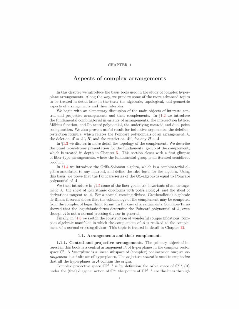
196
Complex Arrangements: Algebra, Geometry, Topology Draft of September 4, 2009 Dan Cohen Graham Denham Michael Falk Hal Schenck Alex Suciu Hiro Terao Sergey Yuzvinsky
Transcript of Complex Arrangements: Algebra, Geometry, Topology Dan Cohen

Complex Arrangements:
Algebra, Geometry, Topology
Draft of September 4, 2009
Dan Cohen
Graham Denham
Michael Falk
Hal Schenck
Alex Suciu
Hiro Terao
Sergey Yuzvinsky

2000 Mathematics Subject Classification. Primary 32S22, 52C35;Secondary 14F35, 20E07, 20F14, 20J05, 55R80, 57M05
Key words and phrases. hyperplane arrangement, fundamental group, cohomologyring, characteristic variety, resonance variety
Abstract. This is a book about complex hyperplane arrangements: theiralgebra, geometry, and topology.

Contents
Preface vii
Introduction ix
Chapter 1. Aspects of complex arrangements 11.1. Arrangements and their complements 11.2. Combinatorics 41.3. Topology 141.4. Algebra 181.5. Geometry 261.6. Compactifications 30
Chapter 2. Cohomology ring 352.1. Arnold-Brieskorn and Orlik-Solomon Theorems 352.2. Topological consequences 382.3. Geometric consequences 382.4. Homology and Varchenko’s bilinear form 412.5. Quadratic OS algebra 47
Chapter 3. Special classes of arrangements 493.1. Generic arrangements 493.2. Reflection arrangements 523.3. Simplicial arrangements 553.4. Supersolvable arrangements 553.5. Hypersolvable arrangements 613.6. Graphic arrangements 62
Chapter 4. Resonance varieties 654.1. The cochain complex determined by a one-form 654.2. Degree-one resonance varieties 694.3. Resonance over a field of zero characteristic 754.4. Nets and multinets 784.5. Bounds on dimH1(A, a) 824.6. Higher-degree resonance 87
Chapter 5. Fundamental Group 895.1. Fundamental group and covering spaces 895.2. The braid groups 905.3. Polynomial covers and Bn-bundles 915.4. Braid monodromy and fundamental group 945.5. Fox calculus and Alexander invariants 96
iii

iv CONTENTS
5.6. The K(π, 1) problem and torsion-freeness 975.7. Residual properties 98
Chapter 6. Lie Algebras attached to arrangements 1016.1. Lie algebras 1016.2. Quadratic algebras, Koszul algebras, duality 1036.3. Lie algebras attached to a group 1056.4. The associated graded Lie algebra of an arrangement 1056.5. The Chen Lie algebra of an arrangement 1066.6. The homotopy Lie algebra of an arrangement 1076.7. Examples 108
Chapter 7. Free Resolutions and the Orlik–Solomon algebra 1097.1. Introduction 1097.2. Resolution of the Orlik-Solomon algebra over the exterior algebra 1107.3. The resolution of A∗ 1167.4. The BGG correspondence 1187.5. Resolution of k over the Orlik-Solomon algebra 1237.6. Connection to DGAs and the 1-minimal model 130
Chapter 8. Local systems on complements of arrangements 1358.1. Three views of local systems 1358.2. General position arrangements 1378.3. Aspherical arrangements 1398.4. Representations ? 1438.5. Minimality ? 1438.6. Flat connections 1438.7. Nonresonance theorems 145
Chapter 9. Logarithmic forms, A-derivations, and free arrangements 1499.1. Logarithmic forms and derivations along arrangements 1499.2. Resolution of arrangements and logarithmic forms 1509.3. Free arrangements 1519.4. Multiarrangements and logarithmic derivations 1529.5. Criteria for freeness 1549.6. The contact-order filtration and the multi-Coxeter arrangements 1559.7. Shi arrangements and Catalan arrangements 157
Chapter 10. Characteristic varieties 15910.1. Computing characteristic varieties 15910.2. The tangent cone theorem 16010.3. Betti numbers of finite covers 16010.4. Characteristic varieties over finite fields 161
Chapter 11. Milnor fibration 16311.1. Definitions 16311.2. (Co)homology 16411.3. Examples 166
Chapter 12. Compactifications of arrangement complements 16712.1. Introduction 167

CONTENTS v
12.2. Definition of M 16712.3. Nested sets 16812.4. Main theorems 171
Bibliography 173


Preface
This is a book about the algebra, geometry, and topology of complex hyperplanearrangements.
Dan CohenGraham Denham
Michael FalkHal SchenckAlex SuciuHiro Terao
Sergey Yuzvinsky
vii


Introduction
In the introduction to [171], Hirzebruch wrote: “The topology of the com-plement of an arrangement of lines in the projective plane is very interesting, theinvestigation of the fundamental group of the complement very difficult.” Muchprogress has occurred since that assessment was made in 1983. The fundamentalgroups of complements of line arrangements are still difficult to study, but enoughlight has been shed on their structure, that once seemingly intractable problemscan now be attacked in earnest. This book is meant as an introduction to somerecent developments, and as an invitation for further investigation. We take a freshlook at several topics studied in the past two decades, from the point of view ofa unified framework. Though most of the material is expository, we provide newexamples and applications, which in turn raise several questions and conjectures.
In its simplest manifestation, an arrangement is merely a finite collection oflines in the real plane. These lines cut the plane into pieces, and understandingthe topology of the complement amounts to counting those pieces. In the case oflines in the complex plane (or, for that matter, hyperplanes in complex ℓ-space),the complement is connected, and its topology (as reflected, for example, in itsfundamental group) is much more interesting.
An important example is the braid arrangement of diagonal hyperplanes in Cℓ.In that case, loops in the complement can be viewed as (pure) braids on ℓ strings,and the fundamental group can be identified with the pure braid group Pℓ. For anarbitrary hyperplane arrangement, A = H1, . . . , Hn, with complement X(A) =Cℓ \ ⋃ni=1Hi, the identification of the fundamental group, G(A) = π1(X(A)), ismore complicated, but it can be done algorithmically, using the theory of braids.This theory, in turn, is intimately connected with the theory of knots and links in3-space, with its wealth of algebraic and combinatorial invariants, and its variedapplications to biology, chemistry, and physics. A revealing example where devel-opments in arrangement theory have influenced knot theory is Falk and Randell’s[132] proof of the residual nilpotency of the pure braid group, a fact that has beenput to good use in the study of Vassiliev invariants.
A more direct link to physics is provided by the deep connections between ar-rangement theory and hypergeometric functions. Work by Schechtman-Varchenko[285] and many others has profound implications in the study of Knizhnik-Zamolod-chikov equations in conformal field theory. We refer to the recent monograph byOrlik and Terao [244] for a comprehensive account of this fascinating subject.
Hyperplane arrangements, and the closely related configuration spaces, areused in numerous areas, including robotics, graphics, molecular biology, computervision, and databases for representing the space of all possible states of a systemcharacterized by many degrees of freedom. Understanding the topology of com-plements of subspace arrangements and configuration spaces is important in robot
ix

x INTRODUCTION
motion planning (finding a collision-free motion between two placements of a givenrobot among a set of obstacles), and in multi-dimensional billiards (describing pe-riodic trajectories of a mass-point in a domain in Euclidean space with reflectingboundary).
CHAPTER 1
Aspects of complex arrangements
In this chapter we introduce the basic tools used in the study of complex hyper-plane arrangements. Along the way, we preview some of the more advanced topicsto be treated in detail later in the text: the algebraic, topological, and geometricaspects of arrangements and their interplay.
We begin with an elementary discussion of the main objects of interest: cen-tral and projective arrangements and their complements. In §1.2 we introducethe fundamental combinatorial invariants of arrangements: the intersection lattice,Mobius function, and Poincare polynomial, the underlying matroid and dual pointconfiguration. We also prove a useful result for inductive arguments: the deletion-restriction formula, which relates the Poincare polynomials of an arrangement A,the deletion A′ = A \H , and the restriction AH , for any H ∈ A.
In §1.3 we discuss in more detail the topology of the complement. We describethe braid monodromy presentation for the fundamental group of the complement,which is treated in depth in Chapter 5. This section closes with a first glimpseof fiber-type arrangements, where the fundamental group is an iterated semidirectproduct.
In §1.4 we introduce the Orlik-Solomon algebra, which is a combinatorial al-gebra associated to any matroid, and define the nbc basis for the algebra. Usingthis basis, we prove that the Poincare series of the OS-algebra is equal to Poincarepolynomial of A.
We then introduce in §1.5 some of the finer geometric invariants of an arrange-ment A: the sheaf of logarithmic one-forms with poles along A, and the sheaf ofderivations tangent to A. For a normal crossing divisor, Grothendieck’s algebraicde Rham theorem shows that the cohomology of the complement may be computedfrom the complex of logarithmic forms. In the case of arrangements, Solomon-Teraoshowed that the logarithmic forms determine the Poincare polynomial of A, eventhough A is not a normal crossing divisor in general.
Finally, in §1.6 we sketch the construction of wonderful compactifications, com-pact algebraic manifolds in which the complement of A is realized as the comple-ment of a normal-crossing divisor. This topic is treated in detail in Chapter 12.
1.1. Arrangements and their complements
1.1.1. Central and projective arrangements. The primary object of in-terest in this book is a central arrangement A of hyperplanes in the complex vectorspace Cℓ. A hyperplane is a linear subspace of (complex) codimension one; an ar-rangement is a finite set of hyperplanes. The adjective central is used to emphasizethat all the hyperplanes in A contain the origin.
Complex projective space CPℓ−1 is by definition the orbit space of Cℓ \ 0under the (free) diagonal action of C∗: the points of CPℓ−1 are the lines through
1

2 1. ASPECTS OF COMPLEX ARRANGEMENTS
the origin in Cℓ. The orbit of (x1, . . . , xℓ) ∈ Cℓ \ 0 is denoted [x1 : · · · : xℓ]. SinceA is central, each hyperplane H ∈ A is a union of lines through the origin, andthus determines a projective subspace of CPℓ−1, also of codimension one. Thisprojective hyperplane will be denoted H . The collection A = H | H ∈ A is calleda projective arrangement. Clearly there is a one-to-one correspondence betweenprojective arrangements in CPℓ−1 and central arrangements in Cℓ. The hyperplanesof A are mutually disjoint precisely when
⋂H∈AH = 0, in which case we say A is
essential. In general, the codimension of⋂H∈AH is called the rank of A, denoted
rk(A). So A is essential if and only if rk(A) = ℓ.Each H ∈ A is the kernel of a nonzero linear functional, αH : Cℓ → C, uniquely
determined by H up to a nonzero scalar multiple. The polynomial
(1.1) QA =∏
H∈AαH
is called the defining polynomial of A. It is homogeneous of degree n = |A|. Theaffine algebraic variety U(A) defined by QA(x1, . . . , xℓ) = 0 is just the union of thehyperplanes in A; the projective variety defined by QA is the union of A.
Most of what we will do is aimed at understanding the topology and geometryof these (embedded) varieties. A standard approach is to study the topology of thecomplement. Thus we define the complement of A by M(A) = Cℓ \⋃H∈AH , and
similarly, M(A) = CPℓ−1 \⋃H∈A H.
There is a simple relationship between M(A) and M(A). The free C∗ actionleaves M(A) invariant, and the quotient is precisely M(A). Thus we have a bundleC∗
M(A)→M(A).
Theorem 1.1. If A is nonempty, then the bundle C∗ M(A) → M(A) is
trivial. In particular,
(1.2) M(A) ∼= M(A)× C∗.
Proof. Let H0 ∈ A. The Hopf bundle C∗ Cℓ \ 0 → CPℓ−1 restricts to
a trivial bundle, C∗ Cℓ \H0 → CPℓ−1 \H0, since the base is diffeomorphic to
Cℓ−1, which is contractible. Hence, a fortiori, the bundle C∗ M(A)→M(A) is
trivial.
1.1.2. Multiarrangements. Sometimes it is convenient to allow the definingpolynomial (1.1) to be unreduced. A multiarrangement (A,m) is an arrangementtogether with a positive integer vector of multiplicities m ∈ ZA
>0. Its definingpolynomial
(1.3) Q(A,m) =∏
H∈AαmH
H
is homogeneous of degree N =∑
H∈AmH . We will call N the multiplicity of(A,m). Clearly the multiarrangement and its underlying reduced arrangementhave the same complement.
1.1.3. Cone and decone. Choosing a particular hyperplane H0 ∈ A, as inthe proof of Theorem 1.1, determines a preferred section of the map M(A) →M(A). The section is given explicitly by [x1 : · · · : xℓ] 7→ αH0(x)
−1(x1, . . . , xℓ) forx = (x1, . . . , xℓ) ∈ Cℓ. The image of this map is contained in the affine hyperplaneS defined by αH0(x) = 1, and coincides with the complement of the union of the

1.1. ARRANGEMENTS AND THEIR COMPLEMENTS 3
affine hyperplanes of S given by H ∩ S for H ∈ A \ H0. Identifying S with Cℓ−1
we obtain (up to linear change of variables) a set of |A| − 1 affine hyperplanes inCℓ−1, which is called the decone of A, and is denoted dA.
It is customary to choose coordinates so that the special hyperplane H0 is givenby xℓ = 0. Then we can identify S with Cℓ−1 via (x1, . . . , xℓ−1, 1) 7→ (x1, . . . , xℓ−1),and the affine hyperplanes of dA are obtained by simply substituting xℓ = 1 in theequations αH(x) = 0 for each H ∈ A \ H0. This procedure is most easily statedin terms of defining polynomials.
Definition 1.2. Suppose H0 ∈ A is given by xℓ = 0. The decone of A relativeto H0 is the collection dA of affine hyperplanes in Cℓ−1 determined by the equation
(1.4) QA(x1, . . . , xℓ−1, 1) = 0.
More precisely, dA is the set of irreducible components of the variety definedby the equation above. Since, by assumption, xℓ divides QA, there are |A| − 1hyperplanes in dA, one for each H ∈ A \ H0. When no confusion is possible,we’ll use H to denote the affine hyperplane in dA corresponding to H ∈ A \ H0.Then, in a sense, H0 will be the “hyperplane at infinity” in Cℓ−1. It is not anelement in dA.
In view of the deconing procedure, we will extend our terminology and notationto affine arrangements, consisting of affine hyperplanes. We will adopt the attitudethat central and projective arrangements are the fundamental objects of study,whereas affine arrangements are a computational tool for the study of projectivearrangements. Indeed, the unnatural choice of one hyperplane H0 from A as thehyperplane at infinity often obscures the true state of affairs.
The discussion leading to the definition of decone gives us the following basicresult.
Theorem 1.3. Let A be a central hyperplane arrangement in Cℓ. The comple-ment of A in CPℓ−1 is diffeomorphic to the complement of dA in Cℓ−1:
M(A) ∼= M(dA).
Corollary 1.4. M(A) ∼= M(dA)× C∗.
In particular, the diffeomorphism type of the complement of dA does not de-pend on the choice of deconing hyperplane.
There is an inverse procedure, called “coning,” by which one reconstructs thecentral arrangement A, up to linear isomorphism, from a decone.
Definition 1.5. Suppose A is an arrangement of n affine hyperplanes in Cℓ,with defining polynomial QA. The cone of A is the central arrangement cA of n+1linear hyperplanes in Cℓ+1 with defining polynomial
QcA(x0, . . . , xℓ) = xn+10 ·QA(x1/x0, . . . , xℓ/x0).
The defining polynomialQA of an affine arrangement need not be homogeneous.The homogeneous polynomial QcA is obtained by “homogenizing” QA relative tothe new variable x0, and then multiplying by x0. Clearly, deconing cA relative tothe hyperplane x0 = 0 yields A. If A is central, the cone of dA coincides with A,up to linear change of coordinates.
Corollary 1.6. If A is an affine arrangement, then M(cA) ∼= M(A)× C∗.

4 1. ASPECTS OF COMPLEX ARRANGEMENTS
Example 1.7. Suppose A is a central arrangement of n lines in C2. Then theprojective arrangement A consists of n points in CP1 ∼= S2. Thus the projectivecomplement M(A) is homotopy equivalent to the bouquet
∨n−1k=1 S
1 of n − 1 cir-cles, and the complement M(A) of the original central arrangement is homotopy
equivalent to(∨n−1
k=1 S1)× C∗ ≃
(∨n−1k=1 S
1)× S1.
The C-linear isomorphism type of an arrangement A in C2 determines (and isdetermined by) the cross-ratios of four-tuples of points in A. On the other hand, forany two central arrangementsA1 andA2 of n lines in C2, there is a homeomorphismφ : C2 → C2 to itself carrying the lines of A1 to those of A2. This homeomorphismcan be constructed so as to be differentiable away from the origin. So the pairs(C2,M(A1)) and (C2,M(A2)) are homeomorphic, and the complementsM(A1) andM(A2) are diffeomorphic, even though A1 and A2 need not be linearly isomorphic.If φ is differentiable at the origin, then Dφ0 will be a linear isomorphism carryingA1 to A2.
1.2. Combinatorics
1.2.1. The intersection lattice. Now let V be a finite-dimensional vectorspace over an arbitrary field k, and let A be a central arrangement of n linearhyperplanes in V . The main combinatorial object associated to A is the intersectionlattice L(A). This is the partially-ordered set whose elements are the linearsubspaces of V obtained as intersections of sets of hyperplanes from A, orderedby reverse inclusion. The ambient vector space V serves as the unique minimalelement of the poset, and
⋂H∈A H is the largest element.
Example 1.8. Probably the best-known hyperplane arrangement is the braidarrangement Aℓ−1, consisting of all the “diagonal” hyperplanes Hij = xi−xj = 0in Cℓ. A defining polynomial for Aℓ−1 is
(1.5) Q(Aℓ−1) =∏
1≤i<j≤ℓ(xi − xj).
Note that the arrangement has rank ℓ− 1: the top element⋂H∈A H of the lattice
is the line x1 = · · · = xℓ. If we project along that line onto the subspace x ∈Cℓ | ∑ xi = 0 ∼= Cℓ−1, we obtain an essential arrangement of rank ℓ − 1 whoseintersection lattice is isomorphic to L(Aℓ−1). In fact more is true: the projectionrestricts to a homotopy equivalence of the complements. (The restriction is theprojection of a trivial C-bundle.)
Intersections of the hyperplanes of Aℓ−1 correspond to partitions of 1, . . . , ℓ,whose blocks indicate which sets of coordinates are equal. In fact L(Aℓ−1) ∼= Π(ℓ),the lattice of partitions of 1, . . . , ℓ, ordered by refinement. Figure 1.1 shows thereal part of the projectivized arrangement A3, together with the intersection latticeΠ(4).
The hyperplanes of the braid arrangement are defined by real linear forms.For this reason, the picture of the real trace of A3 in Figure 1.1 gives us a some-what honest representation of the complex arrangement—at least all the incidencestructure is reflected in the real part. Complex arrangements with real definingforms are called complexified arrangements. This assumption simplifies many ofthe algorithms we present later, e.g., for presentations of the fundamental group.At the same time, complexified arrangements have special geometric, topological,

1.2. COMBINATORICS 5
H12
H13
H23 H34 H24
H14
1234•
123•
12•
∅•
13•6
66
66
6
23•I
II
II
II
I13|24•
24•TTTTTTTTTTTTT
124•
uu
uu
uu
uu
14•I
II
II
II
I
PPPPPPPPPP14|23•
66
66
66
134•
n n n n n n n n n n
34•I
II
II
II
I12|34•
h h h h h h h h h h h h h h h h
66
66
66
234•
j j j j j j j j j j j j j
Figure 1.1. The braid arrangement A3 and its intersection lattice
and combinatorial properties not enjoyed by general complex arrangements. For in-stance, if A is complexified, then M(A) is a Z2-space, and there is a correspondingequivariant theory [262]. There is no known combinatorial or topological charac-terization of complexified arrangements. If A is a complexified arrangement we willwrite AR for the underlying real arrangement; the intersection lattices of A and AR
are isomorphic.
1.2.2. Geometric lattices. A partially ordered set P is said to satisfy thechain condition if for any two comparable elements x, y ∈ P , all maximal linearlyordered chains x = x0 ≺ x1 ≺ · · · ≺ xn = y have the same cardinality. A posetis ranked if it satisfies the chain condition and possesses a unique minimal element0. In this case the rank of x ∈ P , denoted rk(x), is the length of a maximal chain
from 0 to x. Elements of rank one in a ranked poset are called atoms. A poset is alattice if for any pair of elements x, y ∈ P , P contains a (necessarily unique) leastupper bound x∨ y (the join) and a greatest lower bound x∧ y (the meet) of x and
y. A finite lattice also has a unique largest element 1 =∨x∈P x. The rank of P ,
denoted rk(P ), is rk(1).Let A be a central arrangement. The intersection lattice L(A) of A is a ranked
poset. The minimal element 0 is V . The chain condition holds because everyelement is an intersection of hyperplanes. Indeed, this implies that any maximalchain from X to Y has length dim(X)− dim(Y ). In particular, the rank rk(X) isthe codimension of X . For an integer p, let Lp(A) denote those elements of L(A)of rank p.
L(A) is, moreover, a lattice. The join and meet of X,Y ∈ L(A) are given by
X ∨ Y = X ∩ YX ∧ Y =
⋂Z ∈ L(A) | X + Y ⊆ Z.
Definition 1.9. A ranked lattice L is a geometric lattice if
(1) Every element of L− 0 is a join of atoms.(2) rk(x) + rk(y) ≥ rk(x ∨ y) + rk(x ∧ y) for all x, y ∈ L.
Lemma 1.10. The intersection lattice L(A) of a central arrangement A is ageometric lattice.

6 1. ASPECTS OF COMPLEX ARRANGEMENTS
Proof. The first condition is automatic, since in L(A), the join of X and Yis X ∩ Y . The second condition holds because
dim(X + Y ) + dim(X ∩ Y ) = dim(X) + dim(Y ),
and dim(X + Y ) ≤ dim(X ∧ Y ).
The top element 1 = 1A in L(A) is⋂H∈A H , so the rank rk(L(A)) is equal to
rk(A). Suppose A is not essential. Then let Ae =H/1 | H ∈ A
, an arrangement
in V/1. Identifying V with V/1 × 1 gives a bijection between L(A) and L(Ae),since all subspaces contain 1. For complex arrangements, in particular, M(A) is
isomorphic to M(Ae) × 1. Thus every central arrangement has a unique essentialarrangement associated with it, which carries all the important topological andcombinatorial features. (See Example 1.8.)
If A is the projectivization of A, then the elements of L(A) correspond to theintersections of hyperplanes in A, and the rank of X is the codimension of theprojective image X in CPℓ−1. If A is essential, the top element corresponds to theempty intersection, of dimension −1.
Let dA be the decone of A relative to the hyperplane H0. The intersectionsemi-lattice L(dA) of the affine arrangement dA is defined to be the set of nonemptyintersections of hyperplanes in dA, ordered by reverse inclusion. We may identifyL(dA) with a subposet of L(A):
(1.6) L(dA) = X ∈ L(A) | H0 6≤ X.It is still true that L(dA) is a ranked poset, with rk(X) = codim(X). Moreover,
it is clear that the meet exists; indeed, X∧Y is given by the same formula as above.A poset with this property is called a meet semi-lattice. The join X∨Y exists if andonly if X ∩ Y 6= ∅. All maximal elements of L(dA) have the same rank, called the
rank of the affine arrangementA; see [242], Lemma 2.4. It follows that L(dA)∪1is a ranked lattice, where the top element 1 corresponds to the empty intersection.However, L(A)∪1 is not a geometric lattice in general. The intersection poset ofan affine arrangement provides the model for the combinatorial notion of geometricsemi-lattice, see [321]. Every geometric semi-lattice can be embedded in a geometriclattice, in the same way that L(dA) is included in L(A).
1.2.3. Mobius function and Poincare polynomial. An important rolewill be played by the Poincare polynomial of L(A), defined in terms of the Mobiusfunction.
Definition 1.11. The Mobius function, µ : L(A) × L(A) → Z, is defined re-cursively by
(1) µ(X,X) = 1(2)
∑X≤Z≤Y
µ(X,Z) = 0 if X < Y
(3) µ(X,Y ) = 0 otherwise
We will mostly use the one-variable Mobius function, defined by µ(X) =
µ(0, X). Then µ(0) = 1 and, for X > 0, µ(X) = −∑Y <X µ(Y ). In particular,µ(H) = −1 for H ∈ A.

1.2. COMBINATORICS 7
2•
−1•
1•
−1•J
JJ
JJ
JJ
−1•VVVVVVVVVVVVV
1•
−1•
//
//
1•
l l l l l l l l l l
−1•/
//
//
2•
l l l l l l l l l l
//
//
Figure 1.2. A line arrangement and its Mobius function
Definition 1.12. The Poincare polynomial of A is defined as
(1.7) π(A, t) =∑
X∈L(A)
µ(X)(−t)rk(X).
Note that π(A,−1) = 0 by definition of µ, so (1 + t) divides π(A, t).As we shall see later in this chapter, π(A, t) really is the Poincare polynomial
of M(A):
(1.8) π(A, t) =∑
rk(Hi(M(A),Z)) · ti.A sample computation is given in Figure 1.2; for this line arrangement, we findπ(A, t) = 1 + 6t+ 11t2 + 6t3 = (1 + t)(1 + 5t+ 6t2).
1.2.4. Combinatorial complexes. Associated to any (locally finite) posetis its order complex:
Definition 1.13. The order complex of a poset P is the simplicial complexK(P ) whose simplices correspond to chains in P .
If P is a poset and X,Y ∈ P with X ≤ Y , let (X,Y ) and [X,Y ], respectively,denote the open and closed intervals between X and Y , regarded as subposets ofP . It is an easy exercise to show that if a poset has a maximal or minimal element,then its order complex is contractible. On the other hand, Rota observes in [272]that the Mobius function is a (reduced) Euler characteristic of an order complex:for any X,Y ∈ P with X ≤ Y ,
(1.9) µP (X,Y ) = χ(K(X,Y )).
So, from a homological perspective, it is natural to consider the open interval (0, 1)in the intersection lattice of an arrangement A; its order complex is called theFolkman complex F(A).
The homology of the Folkman complex is determined by the Mobius function:in [145], Folkman showed that
Hi(F(A), R) =
0 if i 6= rk(A) − 2
R|µ(1)| if i = rk(A) − 2.
This was later strengthened (by ??): in fact, F(A) is homotopy-equivalent to awedge of spheres, all of dimension rk(A) − 2.

8 1. ASPECTS OF COMPLEX ARRANGEMENTS
For the braid arrangementA3 pictured in Figure 1.1, |L1(A3)| = 6 and |L2(A3)| =7, so F(A) has 13 vertices. Among the rank-two lattice elements, four lie abovethree atoms and three lie above two atoms. Thus there are 18 edges in F (A). Since
F(A3) is connected, H1(F(A3)) is free of rank six, which, as we saw earlier, is equal
to |µ(1)|. (As an exercise, the reader is invited to check that F(A3) is obtained fromthe graph in Figure 1.10 by adding a vertex at the midpoint of each of the threeedges labelled ij, kl, where i, j, k, l ⊆ 1, 2, 3, 4, and the resulting 1-complex ishomotopy-equivalent to a wedge of six circles.)
The Folkman complex F (A) encodes the structure of the cohomology algebraH∗(M,Z), see [240, 340]; it also plays a role in local system cohomology calcula-tions. The atomic complex ∆(L) is a much smaller complex, homotopy equivalentto F(A), that can also be used to model H∗(M,Q). The vertices of ∆(L) are the
atoms of L, and ai1 , . . . , aik is a simplex of ∆(L) if and only if∨kj=1 aij 6= 1. See
[339] for more details on this construction.
1.2.5. Localization and Restriction. Arrangements have natural “subob-ject” and “quotient” constructions. A subarrangement is just a subset; if A is an ar-rangement in V andX is a linear space, the subarrangementAX = H ∈ A : H ⊇ Xis called the localization at X . If X ∈ L(A), it is straightforward to check that
L(AX) is naturally isomorphic to the closed interval [0, X ] in L(A). The arrange-ment AX (in V ) is not essential, unless X is the origin, so it is reasonable to replaceit when necessary with the essential arrangement AeX , an arrangement in V/X (asin §1.2.2.)
On the flip side, for any linear spaceX we may also define an arrangement in X ,called the restriction, by letting AX = H ∩X : H ∈ A \ AX. If X ∈ L(A), one
can check that L(AX) is isomorphic to the closed interval [X, 1]. The arrangementAX is a multiarrangement in a natural way (see §1.1.2): let the multiplicity mK ofK ∈ AX equal the integer |H ∈ A : H ∩X = K|.
With these two constructions, then, any closed interval [X,Y ] in an intersectionlattice L(A) is itself the intersection lattice of an arrangement: L((AY )X) ∼= [X,Y ].
1.2.6. Deletion–Restriction. The Poincare polynomial π(A, t) satisfies a re-cursion similar to the familiar deletion/contraction (Tutte-Grothendieck) recursionfor chromatic polynomials of graphs. The corresponding operations on arrange-ments, called deletion and restriction, comprise a standard approach to inductivearguments in a variety of contexts. In fact deletions and restrictions of an ar-rangement are realizations of deletions and contractions of the underlying matroid,disregarding loops and multiple points; see §1.2.7.
If H is a hyperplane of A, the deletion A′ is the subarrangement A \H of A,and the restriction A′′ is the restriction arrangement AH
This construction arises so frequently in inductive arguments that it meritsnotation:
Definition 1.14. A triple is a set of arrangements (A′,A,A′′) arising fromdeletion/restriction with respect to some H ∈ A.
When working with objects associated to a triple, we write (O′, O,O′′) for(O(A′), O(A), O(A′′). IfA is an arrangement of n hyperplanes in Cℓ, then obviouslyA′ is an arrangement of n−1 hyperplanes, also in Cℓ, whereasA′′ is an arrangementof at most n− 1 hyperplanes in H ∼= Cℓ−1: the natural multiarrangement (§1.1.2)

1.2. COMBINATORICS 9
associated with AH has multiplicity n − 1; however, all hyperplanes that meet Hin the same rank two flat are identified in A′′. For now, we ignore multiplicityissues, so A′′ is simply an arrangement in H ∼= Cℓ−1. Brylawski showed that atriple satisfies a simple recursion:
Theorem 1.15 ([31]). If (A′,A,A′′) is a triple of arrangements, then
(1.10) π(A, t) = π(A′, t) + tπ(A′′, t).
Proof. First, if X ≤ Y ∈ L(A), then
(1.11) µ(X,Y ) =∑
AX⊆B,1B=Y
(−1)|B\AX |.
To prove this, we must show
∑
X≤Z≤Y
∑
AX⊆B,1B=Z
(−1)|B\AX |
=
1, if Y = X
0, otherwise
We consolidate the left hand expression into∑
AX⊆B⊆AY
(−1)|B\AX |.
If X = Y then this is equal to one, and if X < Y , then, letting m = |AY \ AX |, itis equal to
m∑
i=0
(−1)i(m
i
)= 0.
We need a second identity:
(1.12) π(A, t) =∑
B⊆A(−1)|B|(−t)rk(B).
This follows since
π(A, t) =∑
X∈L(A)
µ(0, X)(−t)rk(X) =∑
X∈L(A)
∑
0⊆B,1B=X
(−1)|B|
(−t)rk(X).
Note that 1B is the unique X ∈ L(A) satisfying B ⊆ AX and rk(X) = rk(B). Thenthe last expression is equal to
∑
B⊆A(−1)|B|(−t)rk(B).
We’re ready to prove the deletion/restriction formula. Fix a hyperplane H . FromEquation 1.12, we have
π(A, t) =∑
H∈B⊆A(−1)|B|(−t)rk(B) +
∑
H 6∈B⊆A(−1)|B|(−t)rk(B).
Clearly
π(A′, t) =∑
H 6∈B⊆A(−1)|B|(−t)rk(B).

10 1. ASPECTS OF COMPLEX ARRANGEMENTS
Write µ′′ and rk′′ for the Mobius and rank functions in L′′. We have
∑
H∈B⊆A(−1)|B|(−t)rk(B) =
∑
Y ∈L′′
∑
1B=Y
(−1)|B|
(−t)rk(Y )
= −∑
Y ∈L′′
∑
1B=Y
(−1)|B\AH |
(−t)rk(Y )
= −∑
Y ∈L′′
µ(H,Y )(−t)rk(Y ) by (1.11)
Since µ′′(Y ) = µ(H,Y ) and rk(Y ) = rk′′(Y )+1, the last expression may be rewrit-
ten as −∑µ′′(Y )(−t)rk′′(Y )(−t) = tπ(A′′, t). This finishes the proof.
Example 1.16. Consider the complexified central arrangement B in C3 whoseprojective real part is pictured in Figure 2(a). One computes π(B, t) = 1 + 5t +8t2 +4t3. Observe that B can be obtained from the arrangement A in Example 1.8by deleting any hyperplane, since by symmetry, A′ = B = A \ Hi,j has the sameintersection poset for all i, j. The restriction of A to any hyperplane is a centralconfiguration of three lines in C2 ∼= H (one sees this by noting that each line inFigure 1(a) meets the other lines in three points). Thus, π(A′′, t) = 1+3t+2t2, andso π(A′, t)+ tπ(A′′, t) equals 1+5t+8t2 +4t3 + t(1+3t+2t2) = 1+6t+11t2 +6t3,as expected.
1.2.7. Matroids and dual configurations. If A is a central arrangementin V , then the defining forms αH (with H ∈ A) are vectors in the dual space V ∗,uniquely defined up to scalar multiple. Thus a central arrangement of n distincthyperplanes corresponds to a configuration A∗ of n distinct points in the dualprojective space P(V ∗), and elements of L(A) correspond to projective subspacesof P(V ∗) spanned by subsets of these points.
The primary combinatorial invariant of projective point configurations such asA∗ is the underlying matroid.
Definition 1.17. A matroid M = M(E) is a finite set E, called the groundset, together with a collection C of subsets E, called circuits, satisfying
(1) The empty set is not a circuit;(2) No proper subset of a circuit is a circuit;(3) If C and D are circuits with C 6= D and x ∈ C ∩ D, then (C ∪ D) \ x
contains a circuit.
There are a number of alternate axiom systems for matroids; we have chosen thecircuit axiomatization because it is best suited for our purposes. For each alternatecharacterization, there is a “cryptomorphism” describing how to construct the setof circuits from the alternate data. For example, here is the “independent set”axiomatization for matroids.
(1) The empty set is independent;(2) Any proper subset of an independent set is independent;(3) If C and D are independent sets and |C| > |D| then there exists x ∈ C \D
such that D ∪ x is independent.
(The circuits are then the minimal non-independent sets.) Other axiomatizationsare in terms of bases, rank function, closure operators, bonds or cocircuits, closed

1.2. COMBINATORICS 11
sets, essential flats—in fact there are more than thirty different cryptomorphicdefinitions. The matroid M is actually best thought of as all, or any, of thesestructures on the ground set E.
If E is a projective point configuration, the circuits of the associated matroidare the minimal linearly dependent subsets of E. If E = E(G) is the set of edges ofa finite graph G, the circuits of the associated matroid are the edge-sets of cyclesin the G. In particular a general matroid may have one-element circuits, called“loops”, or two-element circuits, whose elements are said to be “parallel elements”or “multiple points”.
Now let A be an arrangement. A subset B of A is dependent if
(1.13) codim( ⋂
H∈BH)< |B|.
This is equivalent to the existence of a nontrivial linear dependence relation amongthe defining forms αH | H ∈ B. The circuits are exactly the minimal dependentsets. The set of circuits satisfies the axioms above, and thus defines a matroidM(A), with ground set A, which we call the underlying matroid of A. Note M(A)corresponds exactly to the matroid associated to the point configuration A∗ asdescribed above. The matroid M(A) has no loops. For ordinary arrangementsM(A) has no parallel elements. For multiarrangements (§1.1.2) it is natural toconsider an underlying matroid with parallel elements corresponding to multiplehyperplanes.
A subset S ⊂ E is closed in a matroid M(E) if |S ∩C| ≥ |C|− 1 implies C ⊆ Sfor every circuit C ∈ C. The closure S of S ⊆ E is the intersection of all closedsets containing S. Closed sets are also called flats. If E is a projective point config-uration, then the closed sets are the intersections of E with projective subspaces,hence the term “flat”. A matroid also has a rank function defined on subsets S ⊆ Eby letting rk(S) be the size of the largest independent subset of S. In these terms,the closure of S can also be expressed as S = x ∈ E : rkS ∪ x = rkS.
The set of flats of M(E), ordered by inclusion, forms a geometric lattice, whoseatoms are the elements of E. Continuing the analogy with point configurations, flatsof small rank are termed “points,” “lines,” and “planes”. Every geometric latticeis the lattice of flats of some matroid. Using the lattice structure, the closure of a
set S ⊆ E is just the set S =x ∈ E : x ∈ ∧y∈S y
.
It is easy to see that the closed sets in the matroid M(A) are the subarrange-ments of the form AX , in one-to-one correspondence with the elements X ∈ L(A).The lattice of flats of M(A) is isomorphic to L(A). One of the advantages of think-ing of L(A) in terms of the underlying matroid is this: any of these data associatedwith M(A), such as independent sets or rank functions, are sufficient to determineL(A) up to isomorphism, because they determine the underlying matroid.
Two arrangements are combinatorially equivalent if their matroids are isomor-phic, that is, if there is a bijection between the ground sets that sends circuits tocircuits (or, e.g., preserves rank functions). Equivalently, arrangements are combi-natorially equivalent if they have isomorphic intersection lattices.
Another advantage of using the matroid M(A) to encode the combinatoricsof A is that M(A) has a much simpler diagram than the Hasse diagram of L(A).The diagram is just an abstract picture of the dual point configuration A∗. Thehyperplanes of A are represented by points, essential codimension-two flats are

12 1. ASPECTS OF COMPLEX ARRANGEMENTS
Figure 1.3. The matroid of the braid arrangement A3
indicated with lines, and essential codimension-three flats a represented by planes.(We will not define “essential flat” [327]; suffice it to say that two-point lines arenot essential.) This allows us to draw “pictures” of arrangements of rank up tofour, whether they are complexified or not.
Example 1.18. Let A3 be the rank-three braid arrangement from Figure 1.1.Figure 1.3 is the diagram of the underlying matroid.
Example 1.19. The Maclane arrangement in P2C has defining polynomial Q =
xyz(x+ y + z)(x− ωz)(ωx− y)(y + z)(x− ω2y + z), where ω = exp(2π√−1/3).
4 8
27 6
5
1 3
Figure 1.4. The matroid of the MacLane arrangement
Example 1.20. The smallest interesting arrangement of rank four is given byQ = xyzw(x+y+z)(x+y+w). The underlying matroid is illustrated in Figure 1.5.
Figure 1.5. The matroid of the “prism arrangement”
A matroid M = M(E) is said to be realizable over a field k if there exists aconfiguration A∗ of n = |E| points in the projective space Pr−1 = P(kr) whosecircuits are exactly the circuits of M. We have chosen the notation deliberately:

1.2. COMBINATORICS 13
the dual of a hyperplane arrangement is a realization of the underlying matroid. Itis no loss to assume r = rk(M).
Fix a linear ordering of the points of E. Then the realization A∗ of M isrepresented by a n × r matrix R, whose rows are the homogeneous coordinates ofthe points ofA∗, in the given linear order. Note, ifA∗ is the dual of the arrangementA, then the rows of R are the defining linear forms α1, . . . , αn for A, written as rowvectors. This matrix has no zero rows, and no two rows are proportional.
Multiplying R on the left by a nonsingular n × n diagonal matrix, or on theright by a nonsingular m × m matrix, yields a matrix that corresponds to thesame projective configuration, up to linear change of coordinates. The projectiverealization space R(M, k) of M over k is the space of orbits of such matrices underthe left action of (k∗)n and the right action of GL(r, k).
Example 1.21. Let M be the MacLane matroid, whose diagram is pictured inFigure 1.4. Here is a calculation of R(M, k). Suppose R is an 8×3 matrix realizingM, with the labeling of Figure 1.4. We pick a “projective basis” for M, a set offour points every three of which are independent, such as 1, 2, 3, 5. By changingbases we may assume the corresponding rows of R are (1, 0, 0), (0, 1, 0), (0, 0, 1) and(1, 1, 1). Then the orbit of R is uniquely determined by the remaining four rows,modulo scalar multiples.
Since 134 is a circuit, we can then scale the fourth row so it has the form (1, 0, t)for some t 6= 0. Then the remaining rows are determined uniquely determined, interms of t, by the matroid structure. Since 6 is the intersection of the lines 126and 456, the sixth row of R must be (t− 1, t, 0), up to scalar multiple, with t 6= 1.Similarly, the seventh row is (0, 1, 1). As 8 is the intersection of lines 258 and478, the eighth row of R is (1, 1− t, 1). At this point every circuit of M has beenaccounted for, except for 368. For R to realize M, the 368 minor of R must vanish,or, equivalently, t2 − t+ 1 = 0. Thus M is realizable over k if and only if k has aprimitive cube root of 1, and, in this case, R(M, k) consists of two distinct points.
For k = C, these two realizations are complex conjugates. Then the correspond-ing arrangements have diffeomorphic complements, via a real linear diffeomorphism,although the arrangements are not linearly equivalent over C. These arrangementsare used in Rybnikov’s construction of arrangements with isomorphic underlyingmatroids and homotopy inequivalent complements.
Dividing out by the left action, R(M, k) is seen as the quotient of (Pr−1)n
by the diagonal action of GL(r, k). Alternatively, we can divide out by the rightaction of GL(r, k). The orbit space is the Grassmannian Grr(kn); the orbit of Rcorresponds to the column space col(R), an r-dimensional linear subspace of kn.Thus R(M, k) can be identified with the orbit of col(R) under the left action of thetorus (k∗)n.
This last point of view is extremely useful—see [156]. Loosely speaking, itallows us to identify an arrangement of rank r with a point of the GrassmannianGrr(kn). The realization spaces of rank-r matroids yield a stratification of Grr(kn).For this reason, they are often called “matroid strata”. Randell’s lattice isotopytheorem [266] shows that two arrangements which are connected by a path inR(M, k) have diffeomorphic complements. On the other hand, the universalitytheorem of Mnev [227] shows that the topology of these matroid strata can be ascomplicated as that of an arbitrary complex affine variety defined over Q.

14 1. ASPECTS OF COMPLEX ARRANGEMENTS
All of the above depended on first fixing a linear order on the ground setE. Since this ordering is not relevant to the topology of arrangements, we oughtto consider all possible labellings, and mod out by the symmetric group action.Equivalently, we can divide R(M) as defined above by the automorphism group ofM. Thus the true moduli space for an arrangementA with underlying matroid M =M(A) is R(M,C)/Aut(M). For rank-two arrangements these are the unlabeledconfiguration spaces of collections of distinct points in the plane. Very little isknown about the topology of these spaces for higher rank arrangements, even foruniform matroids.
1.3. Topology
1.3.1. Fundamental group. The homotopy type of the complementM(A) islargely determined by its fundamental group, G(A) = π1(M(A), x0). Since M(A)is path-connected, the group G(A) does not depend on the choice of basepoint x0.Since M(A) has the homotopy type of a connected, finite CW-complex, the groupG(A) admits a presentation with finitely many generators and relations.
Example 1.22. As before, let Aℓ−1 be the braid arrangement in Cℓ. Thecomplement M(Aℓ−1) coincides with F (ℓ,C), the configuration space of ℓ distinct,ordered points in C. Thus, as noted by Fox and Neuwirth [116], the fundamentalgroup π1(M(Aℓ−1)) is isomorphic to Pℓ, the Artin pure braid group on ℓ strings.
The arrangement A2 is simply a pencil of 3 lines in C2. As noted in Example1.7, M(A2) ≃ (S1 ∨ S1) × S1; hence, P3
∼= F2 × Z, a product of free groups. Wewill see in Chapter 5 that Pℓ is, in general, not a direct product of free groups, butis an “almost-direct product”.
Using the Lefschetz-type theorem of Hamm and Le [164], one may reduce thecomputation of the fundamental group π1(M(A)) to the case when A is an (affine)line arrangement in C2. Indeed, if A′ is a generic two-dimensional section of A,then the inclusion j : M(A′) → M(A) induces an isomorphism j∗ : π1(M(A′)) →π1(M(A)).
Now, there are several procedures for finding a finite presentation for the fun-damental group of the complement of a line arrangement. All these procedures arebased on the classical method of Zariski [343] and van Kampen [317] for comput-ing fundamental groups of complements of plane algebraic curves. Yet each oneuses in a specific way the particularities of the situation. The first explicit algo-rithm for computing G(A), in the case of a complexified real arrangement, wasgiven by Randell [265]; a generalization to arbitrary arrangements was given byArvola [14], and is recounted in [242]. We will mostly use the braid monodromypresentation, as described by Cohen and Suciu in [55], building on work from[228, 200, 229, 173, 64, 63].
The upshot of all this is that the fundamental group of an arrangement com-plement, G = G(A) has a finite presentation of the form
(1.14) G = 〈x1, . . . , xn | αq(xi) = xi〉,where α1, . . . , αs are certain pure braids in Pn, acting on the generators xi of thefree group Fn via the Artin representation. These braids (one for each intersectionpoint of the lines) can be read off a “braided wiring diagram” associated to A.Finding such a diagram for an arbitrary line arrangement A is, in general, a veryarduous task. Yet, if A is the complexification of a real arrangement, there is a

1.3. TOPOLOGY 15
;
;
Figure 1.6. Pencils and braids
ready-made formula for those braids, depending only on the multiple points, in theorder dictated by a generic projection. See Chapter 5 for full details.
Example 1.23. Suppose A consists of the two coordinate lines, x = 0 andy = 0. Then of course M(A) = C∗ × C∗. In this case, the braid monodromyconsists of a single braid: the full twist on two strands; see the left side of Figure1.6. Hence, G(A) = 〈x1, x2 | x1x2x
−11 = x2〉 = Z2, as expected.
Now add the line y = x, to get a pencil of three lines through the origin.Proceeding as in Example 1.7, we see that M(A) ≃ (S1 ∨ S1)× S1. Alternatively,we find that the braid monodromy consists of a single braid: the full twist on threestrands; see the right side of Figure 1.6. Hence,
G(A) = 〈x1, x2, x3 | x1x2x3x2x−13 x−1
2 x−11 = x2, x1x2x3x
−12 x−1
1 = x3〉.Note that x1x2x3 commutes with all the generators; thus, G(A) ∼= F2 × F1, asexpected.
More generally, if A is a pencil of n lines through the origin of C2, then thebraid monodromy consists of a full twist on n strands, and G(A) ∼= Fn−1 × F1.
In all the examples discussed so far, the fundamental group G(A) can be de-composed as an iterated (semi-)direct product of finitely generated free groups. Aswe shall see, this always happens when the intersection lattice L(A) is supersolvable(or, more generally, hypersolvable). But this is something very special—in general,no such decomposition holds, and the group can be rather complicated.
Figure 1.7. An arrangement of 5 lines
Example 1.24. Consider the arrangement A of 5 lines depicted in Figure 1.7.It turns out that the group G = G(A) has presentation
G =
⟨x1, . . . , x5
∣∣∣∣[x1, x2], [x1, x4], [x1, x5], [x2, x4], [x3, x4],x5x1x3x
−15 x−1
1 x−13 , x3x
−15 x2x5x
−13 x−1
2
⟩
It can be shown that the group G is isomorphic to the celebrated Stallings group.As shown in [300], the group H3(G) is not finitely generated. It follows that G

16 1. ASPECTS OF COMPLEX ARRANGEMENTS
does not admit an Eilenberg-MacLane space K(G, 1) with finitely many 2-cells. Inparticular, the arrangement group G = G(A) cannot be isomorphic to any iterated(semi-) direct product of free groups of finite rank.
1.3.2. Fiber-type arrangements. At this point, we introduce a family ofarrangements with particularly nice structure as well as historical importance.
Definition 1.25. An arrangement A in V is said to be strictly linearly fiberedover AX if X is a line, and the restriction of the projection πX : V → V/X toπX : M(A)→M(AeX) is a fiber bundle projection.
It follows right away that if A is essential, the line X must be an intersectionof hyperplanes, and the fiber is C− m points, for some integer m > 0.remark about suffi-
ciency?Definition 1.26 ([130]).
• The arrangement of one hyperplane is fiber-type.• An arrangement A is fiber-type if there is a line X for which AeX is fiber-
type, and A is strictly linearly fibered over V/X .
Example 1.27. The motivation for such a definition comes from looking atconfiguration spaces; in particular, Fox and Neuwirth [116] noted that the braidarrangement Aℓ is strictly linearly fibered over Aℓ−1, for ℓ ≥ 2. To see this, recallfrom Example 1.8 that
Q(Aℓ) =∏
1≤i<j≤ℓ+1
(xi − xj);
let X be the ℓ + 1st coordinate axis, so that the projection π : V → V/X is givenin coordinates by πX(x1, . . . , xℓ, xℓ+1) = (x1, . . . , xℓ). Then the fiber over a pointx ∈ Cℓ is the set of all (x, t) ∈ Cℓ+1 for which t 6= xi for all 1 ≤ i ≤ ℓ. This isdiffeomorphic to C with ℓ points removed.
Falk and Randell [130] showed that, if A is strictly linearly fibered over AX ,then the bundle map πX has a section. It follows that long exact sequence of thefibration breaks up and gives a split exact sequence of fundamental groups
(1.15) 1 // Fm // π1(M(A))π#
X // π1(M(AX)) // 1,
since π1(C − m points) = Fm, a free group. In other words, π1(M(A)) is iso-morphic to a semidirect product Fm ⋊ π1(M(AX)). Applied recursively, this givesa nice description of the fundamental group of the complement of a fiber-type ar-rangement as an iterated semidirect product of free groups:
Theorem 1.28. If A is a fiber-type arrangement of rank ℓ, then A is anEilenberg-MacLane space, and
π1(M(A)) ∼= Fmℓ⋊ (Fmℓ−1
⋊ (· · ·⋊ Fm1) · · · ),for some integers m1,m2, . . . ,mℓ, where m1 = 1 and m1 +m2 + · · ·+mℓ = |A|.
Falk and Randell also show that the fundamental group of the base acts triviallyon the homology of the fiber, so M(A) (or, equivalently, its fundamental group)have the same Betti numbers as a product of free groups. This will be explored ingreater detail later.

1.3. TOPOLOGY 17
Figure 1.8. A3 is fiber-type. Each fiber has three holes.
Example 1.29. Theorem 1.28 generalizes Fox and Neuwirth’s discovery thatthe pure braid group can be expressed as
Pℓ ∼= Fℓ−1 ⋊ (Fℓ−2 ⋊ (· · ·⋊ F1) · · · ),
since Pℓ = π1(M(Aℓ)).
The fiber-type arrangements also have a combinatorial characterization. Terao [312]showed that they are actually the same as the supersolvable arrangements: we willpick up this thread again in Chapter 3, §3.4.
Example 1.30 (Rank 2). It is easy to see that every rank-2 arrangement isfiber-type. Indeed, if A consists of n ≥ 2 lines in C2, make a linear change ofcoordinates if necessary so that Q = xy(y− c1x)(y− c2x) · · · (y− cn−2x), where theci’s are nonzero and pairwise distinct. Let X be the line with equation x = 0, sothat π−1
X (x) = t ∈ C : Q(x, t) 6= 0, for each fixed x ∈M(AeX). Since x is nonzero,the equation Q(x, t) = 0 always has exactly n − 1 solutions. If one identifiesC− n− 1 points with M(A), we see that the linear fibration
C− n− 1 points // M(A)πX // C∗
is just a choice of splitting of the (restriction of the) Hopf bundle from Theorem 1.1.
Example 1.31 (Rank 3). Given the previous example, a rank-3 arrangementA is fiber-type if and only if it is strictly linearly fibered over AX for some lineX ∈ L(A). The existence of such a line turns out to be easy to detect if thearrangement is drawn as a set of lines in P2: we leave the proof of the followingproposition as an exercise for the reader. Figure 1.8 shows that the arrangementdefined by Q = xyz(x − y)(x − z)(y − z) is strictly linearly fibered with the linedefined by x = y = 0.
Proposition 1.32. If A is an essential arrangement of rank 3, then A is fiber-type if and only if there is a multiple point X in the line arrangement A which isconnected to every other multiple point by a line of the arrangement.

18 1. ASPECTS OF COMPLEX ARRANGEMENTS
1.4. Algebra
1.4.1. The Orlik-Solomon algebra. In this section, we introduce one of themain algebraic objects associated to an arrangement A, the Orlik-Solomon algebraA(A). This algebra is purely combinatorial, in the sense that it is determined byL(A), hence can be defined for any geometric lattice (or matroid). For brevity, wesometimes write A for this algebra, and call it the OS-algebra.
Definition 1.33. Let A = H1, . . . , Hn be a central arrangement, and letE =
∧∗(e1, . . . , en) be the exterior algebra over Z, with generators ei of degree 1.The OS-algebra of A is the quotient algebra
(1.16) A∗(A) = E/I(A),
where I(A) is the OS-ideal, generated by the set
(1.17) ∂eB∣∣B ⊂ A and codim
⋂
H∈BH < |B|.
Here, for a subset B = Hi1 , . . . , Hir of A, we write eB = ei1 · · · eir and ∂eB =∑q(−1)q−1eB\iq.
Theorem 1.34 (Orlik-Solomon [240]). For every arrangement A, there is anisomorphism of graded algebras,
(1.18) A∗(A)∼=−→ H∗(M(A),Z).
Notice that since the hyperplanes of A are distinct, there are no relations of de-gree one; hence A1(A) ∼= E1 ∼= Zn. With this identification, the basis e1, . . . , enof A1(A) is dual to the basis of H1(M(A),Z) given by the meridians of the hy-perplanes. Orlik and Solomon proved the isomorphism by induction on rank andcounting dimensions and a result of Brieskorn [28]; in the next chapter we givea short proof of the Brieskorn and Orlik-Solomon theorems, by way of the Thomisomorphism.
In the definition of A(A), the ring Z can be replaced with an arbitrary commu-tative ring R. The effect on the module structure is negligible: for any such ring,Ap(A) is a free R-module, and its rank is independent of R [178]. The effect onthe ring structure is nontrivial, and will be explored in Chapter 4. When we wantto highlight this aspect, the OS-algebra of A over R is denoted AR(A).
A related algebra is the quadratic Orlik-Solomon algebra A(2)(A), defined asthe quotient of the exterior algebra E by relations of the form ∂eB, for all B ⊂ Asuch that B is dependent and |B| = 3. A(A) is obviously a quotient of A(2)(A),and the two algebras agree in degree ≤ 2. Basically, any invariants of A(A) whichdepend only on L(A)≤2 will be the same for A(A) and A(2)(A).
Example 1.35. For the braid arrangement A3 pictured in Figure 1(a), A(A3)has six generators e1, . . . , e6. If this corresponds to a left to right labelling of thehyperplanes in Figure 1(a), so that e1 ↔ H12 and e6 ↔ H14, then
A(A3) ∼= Λ(e1, . . . , e6)/I(A3),

1.4. ALGEBRA 19
where I(A3) is generated by
∂(e1 ∧ e2 ∧ e3) = e1 ∧ e2 − e1 ∧ e3 + e2 ∧ e3∂(e1 ∧ e5 ∧ e6) = e1 ∧ e5 − e1 ∧ e6 + e5 ∧ e6∂(e2 ∧ e4 ∧ e6) = e2 ∧ e4 − e2 ∧ e6 + e4 ∧ e6∂(e3 ∧ e4 ∧ e5) = e3 ∧ e4 − e3 ∧ e5 + e4 ∧ e5
and the elements ∂(ei∧ej∧ek∧el); these latter elements turn out to be in the idealgenerated by the quadrics, so are superfluous—see Example 2.36. In other words,A(A) = A(2)(A) for this arrangement.
1.4.2. The nbc basis, deletion-restriction. With respect to a fixed order-ing ≺ of the hyperplanes in A, a canonical basis for A is the no broken circuits(or, nbc) basis. If A = H1, . . . , Hn, then (unless otherwise specified) the orderis assumed to be H1 ≻ H2 ≻ · · · ≻ Hn; for brevity we write [i1, . . . , ip] to denotethe ordered tuple Hi1 ≻ Hi2 ≻ · · · ≻ Hip .
Definition 1.36. A broken circuit is a circuit (minimal dependent set) withits smallest element deleted; an nbc set is a set containing no broken circuits.
A word of caution: in the ordering H1 ≻ H2 ≻ · · · ≻ Hn, the smallest elementcorresponds to the largest index. Note that (i) nbc sets are independent, and (ii)every maximal nbc set contains the smallest hyperplane Hn. We will use the termsbroken circuit and nbc set to refer to subsets of A, or as subsets of 1, . . . , nwithout much comment—the meaning should be clear from the context.
Example 1.37. We continue to study the arrangementA3, using the relabelingabove. The sets 1, 2, 3, 1, 5, 6, 2, 4, 6, 3, 4, 5 are dependent, as is any set withfour elements. The broken circuits are thus
[1, 2], [1, 5], [2, 4], [3, 4] ,[1, 2, 3], [1, 2, 4], [1, 2, 5], [1, 3, 4], [1, 3, 5] ,[1, 4, 5], [2, 3, 4], [2, 3, 5], [2, 4, 5], [3, 4, 5] .
Notice that the broken circuits of size three all contain a broken circuit of sizetwo. This property characterizes supersolvable arrangements—the minimal brokencircuits have size two; see [25].
In [23], Bjorner shows that the monomials in the exterior algebra E corre-sponding to broken circuits generate the initial ideal of I(A) with respect to thelexicographic order. The previous example illustrates this; it is clear that in lexorder, the lead monomials of the quadric generators are exactly the broken circuitmonomials. As observed in [178], it follows immediately that the nbc monomialsgive a basis for the Orlik-Solomon algebra as an R-module:
Corollary 1.38. For any commutative ring R, the set[ai1 ∧ · · · ∧ aip ∈ Ap(A) | [i1, . . . , ip] is an nbc set
]
is a free R-module basis for ApR(A).
The nbc basis is the key to understanding the relation between the OS-algebrasin a triple. Let (A′,A,A′′) be a triple with respect to H ∈ A, and suppose |A| = n.Following our convention for a triple, let E′, E,E′′ denote exterior algebras withgenerators corresponding to the hyperplanes of the arrangements A′,A,A′′.

20 1. ASPECTS OF COMPLEX ARRANGEMENTS
Define a map λ : A′ → A′′ via H ′ 7→ H ′ ∩ H . Fix an ordering of A′′, sayH ′′
1 ≻ H ′′2 ≻ · · · ≻ H ′′
k , and order the hyperplanes of A so that
H1 ∩H = · · · = Hi1 ∩H = H ′′1
Hi1+1 ∩H = · · · = Hi2 ∩H = H ′′2
...
Hik−1+1 ∩H = · · · = Hn−1 ∩H = H ′′k
with H = Hn the last (smallest) hyperplane of A. Extend λ to subsets of A′ viaλ([i1, . . . , ip]) = (λ(i1), . . . , λ(ip)). Let i : E′ → E be the obvious inclusion. Tosimplify notation, we write [i1, . . . , ip] for ei1 ∧ · · · ∧ eip . Define j : E → E′′ via
j([i1, . . . , ip]) =
0 if ip 6= n,
[λ(i1) · · ·λ(ip−1)] if ip = n.
Note: λ(i1) · · ·λ(ip−1) may have repeated entries, but is a decreasing sequence.It is obvious that j is surjective and that ji = 0, but in general the sequence
(1.19) 0 // E′ i // Ej // E′′ // 0
is not exact.
Lemma 1.39. i(I ′) ⊆ I and j(I) ⊆ I ′′.Proof. The first statement is immediate. For the second, if i1, · · · , ip is a
dependent set in A, then
j(∂([i1, . . . , ip])) =
p∑k=1
(−1)kj([i1, . . . , ik, . . . , ip])
= 0 if ip 6= n,
j(∂([i1, . . . , ip−1]) · n± [i1, . . . , ip−1])
= ∂([λ(i1), . . . , λ(ip−1)]) if ip = n.
Since codimHi1 ∩ · · · ∩Hip < p, and ip 6= n, we have
codimλ(Hi1 ) ∩ · · · ∩ λ(Hip−1) < p− 1
in Hn. Thus, λ(i1), . . . , λ(ip−1) is dependent.
Theorem 1.40. There is a short exact sequence of R-modules
(1.20) 0 // A′ i // Aj // A′′ // 0 .
Proof. That the sequence above is a complex follows from Equation 1.19 andLemma 1.39. Let (C′, C, C′′) be the free R-modules with bases the respective nbcsets. By Corollary 1.38, to prove the theorem, it suffices to show that the sequence
(1.21) 0 // C′ i // Cj // C′′ // 0 .
is exact. Notice that i(C′) ⊆ C from the choice of Hn as the smallest element ofA, and j(C) ⊆ C′′ from the choice of ordering—if [i1, . . . , ik = n] is nbc, then sois [λ(i1), . . . , λ(ik−1)]. So the sequence above is a complex. To show exactness, itsuffices to show that if ∑
ckj(k, n) = 0

1.4. ALGEBRA 21
with all the [k, n] are nbc, the all the coefficients must vanish. This follows sinceif λ(i) = λ(j), then λ(i) = λ(j) for some i ∈ i, j ∈ j, which implies that [i, j, n]is dependent, hence [j, n] is a broken circuit, contradicting the fact that [j, n] wasnbc.
The map j is of degree −1, so it takes monomials of degree d to monomials ofdegree d− 1. If R = k is a field, then by looking at the graded components we findthat
(1.22) dimkAp = dimkA
′p + dimk A′′p−1,
which shows that the Poincare series of the algebras in a triple satisfy the relation
(1.23) P (A, t) = P (A′, t) + tP (A′′, t).
This identity is of the same form as the identity of Theorem 1.15, so an inductionargument yields:
Corollary 1.41. The Poincare polynomial of the OS-algebra of A equals thePoincare polynomial of A:
(1.24) P (A(A), t) = π(A, t).Example 1.42. The nbc basis for the quadratic component of A(A3) consists
of ei∧ej with [i, j] 6∈ [1, 2], [1, 5], [2, 4], [3, 4], so dimkA2 = dimk E
2−I2 =(62
)−4 =
11, which is indeed the t2 coefficient of π(A, t).
1.4.3. The Brieskorn decomposition. Observe that Corollary 1.41 impliesthe following identity:
(1.25) dim(Ap) =∑
X∈Lp(A)
(−1)pµ(X).
There is a direct sum decomposition of A, indexed by L = L(A), which mirrorsthis numerical identity. This decomposition was originally established by Brieskorn[28] in terms of the cohomology ring of M , and was used in the original proof ofTheorem 1.34 [240]. For us it will provide a useful tool for analyzing resonancevarieties in Chapter 4.
For X ∈ Lp(A), the localization AX (§1.2.5) has rank p. In fact, the sub-arrangement AX of A corresponds to the rank p flat of M(A) corresponding toX .
Denote A(AX) by AX . By Corollary 1.41, applied to AX , the dimension of AXis (−1)pµ(X).
Theorem 1.43. For each p ≥ 0, the following direct-sum decomposition holds:
Ap ∼=⊕
X∈Lp(A)
ApX .
Proof. The crucial point is that the nbc sets of AX are precisely the nbcsets of A which are contained in AX . This holds because AX is a flat of M(A).It then follows from Corollary 1.38 that the natural map AX → A is injective.Moreover, ApX has a basis consisting of the nbc monomials of A of degree p, whichare contained in AX . Finally, since nbc sets are independent, each nbc set of sizep is contained in AX for exactly one X ∈ L of rank p. This defines a partition ofthe nbc monomials if degree p in A, whose blocks are the nbc monomials of AX

22 1. ASPECTS OF COMPLEX ARRANGEMENTS
of degree p, for X ∈ L of rank p. The claimed decomposition then follows fromCorollary 1.38.
A similar argument establishes the following result.
Theorem 1.44. If a ∈ ApX and b ∈ AqY , then ab ∈ Ap+qX∨Y .
As an application, we see that the set of canonical generators of the Orlik-Solomon algebra determines the matroid.
Corollary 1.45. For any S ⊆ A, the monomial eS ∈ A is zero if and only ifS is a dependent set.
Proof. Let p = |S| and q = rk(∨S). Then eS ∈ ApWS , by Theorem 1.44. If S
is dependent, then q < p, so ApWS = Ap(AW
S) = 0. Conversely, if S is independent,
we can order the hyperplanes so that S comes first. Then eS is an nbc monomial,so it must be nonzero by Corollary 1.38.
1.4.4. Projective and affine OS algebras. Let A = H1, . . . , Hn be acentral arrangement in Cℓ with OS-algebra A = AQ(A). The map ∂ : E → E ofDefinition 1.33 is a graded derivation, and satisfies ∂ ∂ = 0. It is not hard to showthat ∂ sends the OS-ideal I to itself, and thus induces a well-defined map on thequotient A = E/I. (See [242, Section 3.1].) Thus we obtain a chain complex
(1.26) 0 // Aℓ∂ // Aℓ−1
∂ // · · · ∂ // A1 ∂ // A0 // 0 .
Note that ∂ei = 1 for the standard generators ei.
Lemma 1.46. The complex (A, ∂) is acyclic.
Proof. Suppose a ∈ A with ∂a = 0. Let b = e1a. Then ∂b = (∂e1)a−e1(∂a) =a.
Let A be the projectivization of A. The projective OS-algebra of A, writtenA(A), is, by definition, the kernel of ∂ : A → A. Since ∂ is a derivation, A(A) isa subalgebra of A. Recall A[−n] denotes the graded algebra obtained from A byshifting degrees by n, that is, A[−n]p = Ap−n.
Theorem 1.47. Let A be an arrangement, with OS-algebra A = A(A) andprojective OS-algebra A = A(A). Then:
(1) A = im ∂.(2) There is a short exact sequence of graded vector spaces
0 // A // A∂ // A[−1] // 0 .
(3) Ap ∼= Ap ⊕ Ap−1.(4) A ∼= A⊗ (C⊕ C[−1]).
Proof. The first statement is immediate from the exactness of (1.26), provedin Lemma 1.46. The acyclicity of (A, ∂) also implies that for each p, we have ashort exact sequence
(1.27) 0 // ker ∂ // Ap // im ∂ // 0 ,
which yields
(1.28) 0 // Ap // Ap // Ap−1 // 0 .

1.4. ALGEBRA 23
This proves (2). This sequence splits. Indeed, define s : im(∂)→ A by s(a) = ana.Then, for a = ∂b, we have ∂ s(a) = ∂(an∂b) = (∂an)(∂b)−an∂∂b = a. This yieldsthe direct sum decomposition (3), while (4) is just a restatement of (2).
Corollary 1.48. The algebra A(A) is generated by the subspace
n∑
i=1
aiei |n∑
i=1
ai = 0
of A1.
Proof. Observe that ∂(ei1 · · · eip) = (ei1 − ei2) · · · (eip−1 − eip). The assertionfollows from (i) above.
The Poincare polynomial of the projective arrangement A is defined by π(A, t) =∑ℓ−1i=0 dimAi(A)ti.
Corollary 1.49. (1 + t)π(A, t) = π(A, t).Theorem 1.50. The projective OS-algebra A(A) is isomorphic to the cohomol-
ogy of the projectivized complement M(A).
Proof. The projection M(A) → M(A)/C∗ = M(A) induces an injectionH∗(M(A)) → H∗(M(A)). The image is the subcomplex represented by forms
whose contraction along the Euler vector field θ =∑ℓ
i=1 xi∂∂xi
vanishes [84]. The
map ∂ corresponds to contraction along θ under the isomorphism of A(A) with
H∗(M): this follows from the fact that dαi
αi(θ) = 1. Thus the subalgebraH∗(M(A))
of H∗(M(A)) corresponds to ker(∂) = A(A).
The definition of the section s : Ap−1(A) ∼= im(∂)→ Ap in the proof of Propo-sition 1.47 depends on the selection of Hn ∈ A as a distinguished hyperplane. Thisdetermines an affine chart on CPℓ−1 and allows us to identify M(A) with the com-plement M(dA) of the corresponding decone of A; see 1.1.3. At the same time thischoice yields a presentation of the projective OS-algebra A(A), with generatorsei := ei − en. The relations are easy consequences of the OS relations. AssumeS = i1, . . . , ip ⊆ 1, . . . , n− 1, and write eS = ei1 · · · eip ∈ Ap.
(1) If⋂i∈S Hi 6⊆ Hn and S is dependent (in A), then ∂eS = 0.
(2) If⋂i∈S Hi ⊆ Hn, then eS = 0.
This presentation can be described in terms of the affine arrangement dA, asin the following definition.
A collection of affine hyperplanes is dependent if and only if its intersection isnon-empty and has codimension greater than the number of hyperplanes.
Definition 1.51. The Orlik-Solomon algebra A(dA) of the affine arrangementdA = H1, . . . , Hn−1 is the quotient of the exterior algebra E on generatorse1, . . . , en−1 by the ideal I generated by
∂eS : S is dependent ∪eS : S
⋂
H∈SH = ∅
.
It is a simple matter to show that A(dA) is isomorphic to A(A), identifyingei with ei − en. The two cases above correspond to the partition of the dependentsets of A according to whether or not they contain Hn.

24 1. ASPECTS OF COMPLEX ARRANGEMENTS
Suppose αi : Cℓ → C is a homogeneous linear form defining the hyperplaneHi ∈ A, and suppose we have chosen coordinates so that αn(x) = xℓ. Thenthe corresponding affine hyperplane Hi ∈ dA is the zero locus of the affine func-tional αi : Cℓ−1 → C given by αi(x1, . . . , xn−1) = αi(x1, . . . , xℓ−1, 1). Moreover,the diffeomorphism M(A) → M(dA) is given by [x1 : · · · : xℓ] 7→ (x1
xℓ, . . . ,
xℓ−1
xℓ).
Piecing this together, it is straightforward to confirm that the logarithmic one-formd log(αi) pulls back to d log(αi)−d log(αn) under the map induced by the compositeM(A)→M(A)/C∗ = M(A)→M(dA). Then, applying Theorem 1.50, we obtainthe following result (see [242] for an alternative approach).
Corollary 1.52. The affine OS algebra A(dA) is isomorphic to the coho-mology H∗(M(dA)), with generators corresponding to the logarithmic one-formsd log(αi).
Using the presentation 1.51 and Theorems 1.47 and 1.38 one can construct annbc-basis for A(dA) ∼= A(A). A broken circuit for dA is a minimal dependent setwith its first element deleted. (By definition, a dependent set of affine hyperplaneshas nonempty intersection.) An nbc set is a set containing no broken circuits. Itis easy to see that S ⊆ H1, . . . , Hn−1 = A is an nbc set if and only if Hi | i ∈S ∪ Hn is an nbc set for A. The analogue of Corollary 1.38 holds for A(dA);again, see [242, Section 3.2].
Theorem 1.53. The set aS | S ∈ nbc(dA) is a basis for A(dA) ∼= A(A).
This result can be used in turn to construct a Brieskorn decomposition forA(A). We will need this in Chapter 4. Let L(dA) = X ∈ L(A) | Hn 6≤ X be theintersection semi-lattice of the affine arrangement dA. Note that each nbc set ofsize p in dA intersects in an element of rank p in L(dA).
Corollary 1.54. Ap(A) ∼=⊕
X∈Lp(dA)Ap(AX).
The collection of all nbc sets of A form a simplicial complex, also denotednbc(A), and perversely called the broken circuit complex. The number of p-simplices of nbc(A) is equal to dim(Ap(A). Since Hn is in every maximal nbc set,the complex nbc(A) is a cone, with apex Hn. The base of the cone is called thereduced broken circuit complex nbc(A). Its simplices are precisely the nbc sets of
the decone dA of A relative to Hn, as described above. That is, nbc(A) = nbc(A).We will need the following structural result in later chapters. The reader is
directed to [347] for the proof.
Theorem 1.55. Let A be an arrangement. Then:
(i) nbc(A) is homotopy equivalent to the order complex |L(dA)| of the inter-section semi-lattice of dA.
(ii) nbc(A) is a pure, shellable (ℓ− 2)-complex, hence is homotopy equivalentto a bouquet of (ℓ− 2)-spheres.
The number of spheres in the bouquet is equal to the beta invariant of A,discussed in the next paragraph. There is a natural basis for the cohomologyHℓ−2(nbc(A)), indexed by so-called β nbc bases of A (the homology facets for theshelling), and this basis is used to construct bases for the cohomology of “non-resonant” local systems in Chapter 8. See [134].

1.4. ALGEBRA 25
1.4.5. Euler characteristics and irreducible arrangements. If A is acentral arrangement, then the Euler characteristic of the complement vanishes.Indeed, M(A) ∼= M(A)× C∗, and so χ(M(A)) = χ(M(A))χ(C∗) = 0.
The Euler characteristic of the projective complement M(A) is given by
(1.29) χ(M(A)) = π(A,−1) = limt→−1
π(A, t)1 + t
.
The right-hand side is equal to (−1)rk(A)−1β(A), where β(A) is the beta invariantof the underlying matroid of A. If A is a complexified real arrangement then β(A)is the number of bounded regions in the complement M(dA)∩Rℓ−1 of any deconeof A; see [344].
Definition 1.56. Let A1 and A2 be central arrangements in Cℓ and Cm, withdefining polynomials Q1(x1, . . . , xℓ) and Q2(x1, . . . , xm), respectively. The productarrangementA1×A2 is the arrangement in kℓ+m ∼= kℓ×km with defining polynomial
Q(x1, . . . , xℓ+m) = Q1(x1, . . . , xℓ)Q2(xℓ+1, . . . , xℓ+m).
We see that A1 × A2 consists of the hyperplanes H × km for H ∈ A1, andkℓ ×H for H ∈ A2.
Proposition 1.57. Suppose A = A1 ×A2. Then
(i) M(A) ∼= M(A1)×M(A2).(ii) π(A, t) = π(A1, t)π(A2, t).(iii) M(A) ∼= M(A1)×M(A2)(iv) β(A) = 0, provided both A1 and A2 are nonempty.
Proof. Using the notation from Definition 1.56, we have (x1, . . . , xℓ+m) ∈M(A) if and only if Q(x1, . . . , xℓ+m) 6= 0, if and only if Q1(x1, . . . , xℓ) 6= 0 andQ2(xℓ + 1, . . . , xℓ+m) 6= 0, i.e., (x1, . . . , xℓ) ∈ M(A1) and (xℓ+1, . . . , xℓ+m) ∈M(A2). This proves assertion (i).
Assertion (ii) follows from Corollary 1.41 and Theorem 2.4. To prove the thirdassertion, we observe that M(dA) and M(A1) ×M(dA2) are complements of thesame divisor, the zero locus of Q1(x1, . . . , xℓ)Q2(xℓ+1, . . . , xℓ+m−1, 1), by equa-tion (1.4). Since M(dA) ∼= M(A) and likewise for A2, the assertion follows. Thisin turn implies (iv), since M(A1) has Euler characteristic zero, by (1.2).
In fact the intersection lattice L(A1 ×A2) is isomorphic to the product posetL(A1)× L(A2) ([245]?), which implies (ii) and (iv) above.
Definition 1.58. A central arrangement A is irreducible if A cannot be ex-pressed as a product of two nonempty arrangements. Similarly, a flat X ∈ L(A) isirreducible if the arrangement AX is irreducible.
According to Theorem 1.57(iv) an irreducible arrangement has nonzero betainvariant. The converse of this statement is also true. This is a purely combinatorialresult, which won’t be used in the sequel; see [245] or [244] for proof.
Theorem 1.59. A central arrangement A is irreducible if and only if β(A) 6= 0.
Proposition 1.57(iii) was used in [114] to construct pairs of projective arrange-ments with non-isomorphic matroids but isomorphic OS-algebras. Suppose A1 andA2 are arbitrary central arrangements in Cℓ and Cm, with defining polynomials

26 1. ASPECTS OF COMPLEX ARRANGEMENTS
Q1(x1 . . . , xℓ) and Q2(y1, . . . , yℓ) respectively. Let A0 be the arrangement consist-ing of the hyperplane 0 in C. We define a new arrangement A in Cℓ+m−1 asfollows: change variables so that xℓ = 0 defines a hyperplane in A1, and ym = 0 de-fines a hyperplane in A2. Then let A be the arrangement whose defining polynomialis obtained by setting xℓ = ym in the product Q1Q2. More precisely,
QA(x1, . . . , xℓ, y1, . . . , ym−1) = Q1(x1, . . . , xℓ)Q2(y1, . . . , ym−1, xℓ).
The arrangement A is called the parallel connection of A1 and A2 along the hyper-planes xℓ = 0 and ym = 0: it contains “copies” of A1 and A2 in which these twohyperplanes are identified. We will write A = A1 ×H A2.
Theorem 1.60 ([114]). The central arrangements (A1×HA2)×A0 and A1×A2
have diffeomorphic complements and isomorphic OS-algebras.
Proof. We show the projectivized complements are diffeomorphic, and thenapply Theorem 1.1. We have
M( ¯A1 ×A2) ∼= M(A1)×M(A2) ∼= M(A1)×M(A2)× C∗,
by Proposition 1.57(iii) and Theorem 1.1.On the other hand, when we decone (A1 ×H A2) × A0 along the identified
hyperplane xℓ = 0, we get the affine arrangement defined by
Q1(x1, . . . , xℓ−1, 1)Q2(y1, . . . , yℓ−1, 1),
whose complement is clearly diffeomorphic to M(dA1) × M(dA2) ∼= M(A1) ×M(A2). Since M(A0) = C∗, the result follows immediately.
Corollary 1.61. For each positive integer n, there exist n combinatoriallyinequivalent arrangements with diffeomorphic complements and isomorphic OS-algebras.
The corollary is established by carefully choosing A1 and A2, such that thereare n combinatorially distinct parallel connections along different choices of hy-perplanes. See [114] for details. The first isomorphism of OS-algebras of combi-natorially distinct arrangements was found by L. Rose and H. Terao [242], usingcandidates exhibited in [120]. Subsequently it was shown in [121] that the com-plements are homotopy equivalent [121]. These examples are shown in Figure 1.9.The complements are not homeomorphic, by a result of T. Jiang and S.-T. Yau[179]. These are sections (see Section 3.1) of two rank-four arrangements whosecomplements are diffeomorphic by Theorem 1.60.
1.5. Geometry
1.5.1. The log complex. If X is a complex manifold andD =∑Di a divisor
such that the Di are smooth and meet transversally (a normal crossing divisor),then associated toD is the sheaf Ωp logD) of meromorphic p-forms with logarithmicpoles on D. If q is a point where D1, . . . , Dm meet, then in a sufficiently smallneighborhood U of q we may choose local coordinates z1, . . . , zm on U so D isdefined on U by the vanishing of z1 · · · zm. Then Ωp logD)(U) is generated byp-forms in the holomorphic 1–forms and the logarithmic differentials dz1
z1, . . . , dzm
zm.
The sheaves Ωp(logD) are locally free ([71]), and a computation shows that
d(Ωp(logD)) ⊆ Ωp+1(logD).

1.5. GEOMETRY 27
Figure 1.9. Projective arrangements with homotopy equivalent complements
The resulting complex is the log complex, and Grothendieck’s algebraic de Rhamtheorem ([161], §3.5) shows that for the complement M = X \D, the cohomologyof this complex computes Hi(M,C). Deligne introduced Ωp(logD) to define mixedHodge structures. In [274], Saito gave a generalization which dispenses with thenormal crossing hypothesis. Our interest will be in the case where X is P(V ), andD is a hyperplane arrangement: for the remainder of this chapter A is central.
Example 1.62. The rank–two braid arrangement A2 has defining polynomial
(x − y) · (x − z) · (y − z). Write A2 = H1, H2, H3, and denote ωi = d(Hi)Hi
. Wethen have
ω1ω2 − ω1ω3 + ω2ω3 = d(x−y)x−y
d(x−z)x−z −
d(x−y)x−y
d(y−z)y−z + d(x−z)
x−zd(y−z)y−z = 0,
and there are no other relations among the ωi’s, except for the standard skew-commutativity relations. In particular, the logarithmic forms satisfy exactly thesame relations as those satisfied by the Orlik-Solomon algebra. This is essentiallythe content of Brieskorn’s theorem, which is proved in Chapter 3.
Definition 1.63. Let S = Sym(V ∗) and F the field of fractions of S, and letΩpS and ΩpF be free modules (over S and F , respectively) on the p-forms. If Q is adefining polynomial for A, then the module of logarithmic p-forms with poles alongA is the submodule Ωp(A) of ΩpF defined by
(1.30) Ωp(A) = ω ∈ ΩpF | Qω ∈ ΩpS and Qdω ∈ Ωp+1S .
The module of A-derivations Dp(A) is the submodule of Λp(DerC S) defined by
(1.31) Dp(A) = θ ∈ Λp(DerC S) | θ(Q, f2, . . . , fp) ∈ 〈Q〉, ∀fi ∈ S.The modules Dp(A) and Ωp(A) are graded by the degree of the polynomial
coefficients. It is easy to see that D1(A) has a direct sum decomposition asD1
0(A)⊕S(−1), where D10(A) is the kernel of the Jacobian matrix of Q and S(−1)
corresponds to the Euler derivation. Correspondingly, we have a decompositionΩ1(A) ∼= Ω1
0(A)⊕ S(1).
Example 1.64. The polynomial Q = x · y · (x − y) defines a configuration of3 points in P1. The Jacobian ideal is a complete intersection defined by 〈2xy −y2, x2 − 2xy〉, so D1(A) has basis x ∂
∂x + y ∂∂x and (2xy − y2) ∂∂y − (x2 − 2xy) ∂∂y .
Thus, D1(A) ∼= S(−1) ⊕ S(−2). For the configuration of 3 lines in P2 defined by

28 1. ASPECTS OF COMPLEX ARRANGEMENTS
the vanishing of xyz, the Jacobian ideal 〈yz, xz, xy〉 has syzygies
x 0−y y0 −z
which correspond to derivations x ∂∂x − y ∂
∂y and y ∂∂y − z ∂
∂z , so D1(A) ∼= S(−1)3.
1.5.2. Arrangements which are normal crossing. The modules Ωp(A)
are graded, so define sheaves on P(V ); as usual let Ω1(A) denote the sheaf associatedto Ω1(A). An arrangement A is generic exactly when A is a normal crossingdivisor. After a change of coordinates, we may assume the first ℓ hyperplanes are
the coordinate hyperplanes; for i ∈ 1, . . . , n − ℓ write li =∑ℓj=1 ai,jxj for the
remaining hyperplanes. In [346], Ziegler gives a free resolution for Ω1(A) for suchan arrangement:
0 // Sn−ℓτ // S(1)n // Ω1(A) // 0 ,
where τ is given by
a1,1x1 · · · · · · an−ℓ,1x1
.... . .
. . ....
a1,ℓxℓ · · · · · · an−ℓ,ℓxℓ−l1 0 · · · 00 −l2 · · · 0...
. . .. . . 0
0 · · · 0 −ln−ℓ
Dolgachev and Kapranov give a presentation for Ω1(logA) in Corollary 3.4 of[99]. An easy application of the snake lemma shows that Ω1(logA) is the sheafassociated to Ω1
0(A)(−1). While this follows from the local description, the pointis that the gradings are a bit different. In general, the relation between a gradedmodule N and the associated sheaf N is given by the exact sequence (see [107],Theorem A.4.1)
(1.32) 0 // H0m(N) // N // ∑
v∈ZH0(N (v)) // H1
m(N) // 0 ,
where H∗m(N) denotes the local cohomology of N . The next lemma shows that in
fact
(1.33) D1(A) ≃⊕
i
H0(D1(A)(i)).
Lemma 1.65. For every central arrangement A ⊆ Cℓ with ℓ ≥ 2, depth Ωp(A) ≥2 and depthDp(A) ≥ 2, for every p, 1 ≤ p ≤ ℓ.
Proof. We prove the result for Ωp(A). It follows from Definition 1.63 thatΩp(A) is torsion-free and therefore depth Ωp(A) ≥ 1. Let m = 〈x1, . . . , xℓ〉. Itsuffices to show that if 0 6= a ∈ S and ω ∈ Ωp(A) are such that mω ⊂ aΩp(A),then ω ∈ aΩp(A). Note that since depthS ≥ 2 and the S-modules ΩiS are free, iffor τ ∈ ΩiK and 0 6= b ∈ S we have m τ ⊂ bΩiS , then τ ∈ ΩiS .
By definition, mQω ⊂ aΩpS and the above observation gives Qω/a ∈ ΩpS . For
every f ∈ m we also have Qd(fω/a) ∈ Ωp+1S . Since
Qd(fω/a) = df ∧Qω/a+Qfd(ω/a),

1.5. GEOMETRY 29
and Qω/a ∈ ΩpS , we find that mQd(ω/a) ⊂ Ωp+1S . One more application of the
observation gives Qd(ω/a) ∈ Ωp+1S , hence ω/a ∈ Ωp(A).
Equation 1.33 follows from the Lemma 1.65 and Equation 1.32, because themodules Hi
m(N) vanish for i < depth(N).In [274], Saito showed that the evaluation map
Ω1(A) ×D1(A)→ S
induced by dxi ⊗ ∂/∂xj = δij is a perfect pairing. Then Lemma 1.65 can be usedto show there is also a perfect pairing between the modules Ωp(A) and Dp(A).Should we mention Residue sequence here?
1.5.3. Relating logarithmic forms and π(A, t). An arrangement A is freeif D1(A) is a free S-module. In [310], Terao proved:
Theorem 1.66. If A is a free arrangement, then π(A, t) =∏
(1 + nit), wherethe ni are the degrees of the generators of D1(A).
In Example 1.64, we saw that D1(A2) ≃ S(−1) ⊕ S(−2), and from Example1.62 it is easy to see that π(A2, t) = 1+3t+2t2. Terao’s theorem may be generalizedas follows: let P (M,x) denote the Hilbert series of a graded S-module M . Then in[297], Solomon and Terao proved:
Theorem 1.67.
χ(A, t) = (−1)ℓ limx→1
∑
p≥0
P (Dp(A);x)(t(x − 1)− 1)p.
This result can be generalized to vector bundles on projective space:
Theorem 1.68 ([233]). For every rank r bundle E on Pℓ−1,
ct(E) = limx→1
(−1)rtr(1− x)ℓ−rr∑
i=0
P (H0∗ (
i∧E);x) ·
(x− 1
t− 1
)i,
where ct is the Chern polynomial.
Following Yuzvinsky [337], we will say that an (essential, central) arrangementA is locally free if for every X ∈ LA with rkX < dimV , the arrangement AX isfree. In [337], Yuzvinsky proves that for such arrangements the Hilbert polynomialof D1(A) is a combinatorial invariant. As a consequence, Theorem 1.66 extends tothe locally free case:
Theorem 1.69. If Ω1(A) is locally free of rank ℓ, then
π(A, t) = ct(Ω1(A)) mod tℓ.
So when Ω1(A) is locally free, applying this theorem and Hirzebruch-Riemann-Roch yields an explicit expression for the Hilbert polynomial of Ω1(A) or D1(A) interms of π(A, t). The modules Ω1(A) and D1(A) are not combinatorial; in [346],Ziegler discovered a pair of combinatorially equivalent arrangements consisting of 9lines in P2, with non-isomorphic modules of derivations. There is also a very simplegeometric description:

30 1. ASPECTS OF COMPLEX ARRANGEMENTS
Example 1.70. In P2, form a linearly generic hexagon, and connect oppositevertices. Since the hexagon is not symmetric, the only non-normal crossings are atthe six vertices of the hexagon. The behavior of D1(A) depends on whether or notthe vertices of the hexagon lie on a smooth conic. The free resolution for D1
0(A)for the arrangement with vertices on a conic is:
0 // S(−7)⊕ S(−8) // S(−5)⊕ S3(−6) // D10(A) // 0 ,
while the free resolution of D10(A) for the arrangement with vertices not on a conic
is:
0 // S4(−7) // S6(−6) // D10(A) // 0 .
In [337], Yuzvinsky shows that in the parameter space for arrangements witha fixed intersection lattice, the set of free arrangements is Zariski-open. So it isnatural to expect special behavior of D1(A) to occur on an algebraic set, exactlyas in the previous example. In [336] Yuzvinsky constructs a submodule of Ω1(A)from elements of L2(A); but this module is not typically equal to Ω1(A). Freenessis a delicate property, and one of the most famous open questions is:
Conjecture 1.71 (Terao). For an arrangement A over a field of characteristiczero, freeness of D1(A) depends only on the combinatorics of A.
There are a number of tools available for proving that an arrangement is free,all of which will be explored in more detail in Chapter 9. We close this sectionby sketching two of them. The first method is based on the deletion-restrictionoperation described in §1.2.
Theorem 1.72 (Terao’s Addition-Deletion Theorem, [308]). Let (A′,A,A′′)be a triple. Then any two of the following imply the third
• D1(A) ∼=⊕n
i=1 S(−bi)• D1(A′) ∼= S(−bn + 1)⊕⊕n−1
i=1 S(−bi)• D1(A′′) ∼=
⊕n−1i=1 S(−bi)
A second criterion for freeness is special to the case of line arrangements; tostate it we need to define freeness for multiarrangements. If (A,m) is a multiar-rangement, the module of derivations is defined to be those derivations θ such thatlmi
i divides θ(li). As shown by Ziegler in [345], freeness of multiarrangements isnot combinatorial.
Theorem 1.73 (Yoshinaga’s multiarrangement criterion, [329]). An arrange-ment A ⊆ P2 is free if and only if π(A, t) = (1 + t)(1 + at)(1 + bt) and, for allH ∈ A, the multiarrangement A|H has minimal generators in degree a and b.
1.6. Compactifications
1.6.1. Motivation: cohomology of configuration spaces. The comple-ment M(A) ⊆ Pℓ−1 of a projective arrangement has one obvious compactification:Pℓ−1. This compactification is not very useful. In this section we give a briefoverview of a much better compactification of M(A), which will be treated in de-tail in Chapter 12. First, a bit of history. Example 1.22 describes the configurationspace F (ℓ,C) of ℓ distinct points in C. Since C1×· · ·×C1 ∼= Cℓ, the condition that

1.6. COMPACTIFICATIONS 31
the points are distinct implies that the hyperplanes V (xi − xj) must be avoided.Hence
F (ℓ,C) = Cℓ \M(Aℓ−1),
where Aℓ−1 is the braid arrangement from Example 1.8. If X is a smooth algebraicvariety, the configuration space of ℓ is defined exactly as above, with X replacingC1. In [154], Fulton and MacPherson construct a compactification X [ℓ] of theconfiguration space F (X, ℓ), so that
• X [ℓ] is smooth.• F (X, ℓ) is the complement in X [ℓ] of a smooth, normal crossing (SNC)
divisor, which is explicitly determined.
If U is the complement of a union of smooth divisors D1, . . . , Dk with normalcrossings in a smooth compact variety X , then Morgan’s pioneering work in [230]allows us to get a handle on the cohomology of U . In particular, Morgan constructsa differential graded algebra (more on this in Chapter 7), whose minimal model inthe sense of Sullivan [305] is the minimal model for H∗(U). In short, a compacti-fication X of U in which X \U is a SNC-divisor is very useful; for example, Fultonand MacPherson use this to give explicit descriptions for the cohomology rings ofX [ℓ] and F (X, ℓ). A key point to make is that while X can be very complicated,the combinatorial data involved in Fulton–MacPherson’s work is exactly that of thebraid arrangement.
The same ideas arising in [154] are central to work of De Concini and Pro-cesi [68] on wonderful models for a subspace arrangement A. De Concini–Procesiconstruct a compactification of M(A) ⊂ Cℓ by taking the closure of the graph
M(A) −→ Cℓ ×∏
D∈GP(Cℓ/D),
where the map is inclusion on the first factor is inclusion, and the restriction ofthe projection Cℓ \ D to P(Cℓ/D) on the second factor. The set G is a buildingset: a subset of the intersections of A, satisfying certain properties described below.DeConcini and Procesi call the resulting compactification of M(A) a “wonderfulmodel”; it enjoys the same properties as the Fulton-MacPherson compactificationof F (X, ℓ).
Recent work of Feichtner and Kozlov [139] gives an abstraction of these con-structions to a purely combinatorial (lattice–theoretic) setting.
1.6.2. Building sets and nested sets. Let L be a meet semi-lattice: anytwo elements x, y ∈ L have a greatest lower bound x ∧ y, called the meet of x andy. A poset is irreducible if it is not the product of two other posets (the productX × Y of posets X and Y consists of pairs (x, y), with order (x′, y′) < (x, y) iffx′ < x, y′ < y). For a given L, let I denote irreducible elements in L and for x ∈ L,D(x) the set of maximal elements in I ∩L≤x. An easy lemma shows that any poset
possessing a unique minimal element 0 admits a unique finest decomposition:
[0, x] ≃m∏
j=1
[0, yj], where y1, . . . , ym = D(x).
Definition 1.74. A building set is a subset G ⊆ L such that for all x ∈ L,
maxG≤x = x1, . . . , xm satisfies [0, x] ≃m∏
j=1
[0, xj ]

32 1. ASPECTS OF COMPLEX ARRANGEMENTS
3412
12323
24
13
13414
234124
Figure 1.10. Nested sets for A3: the link of 1
If G is a building set, then G must contain all irreducible x ∈ L.
Definition 1.75. A subset N of a building set G is called nested if for any setof incomparable elements x1, . . . , xp ⊆ N with p ≥ 2, the join x1 ∨ x2 ∨ · · · ∨ xpexists in L, but is not in G.
The nested sets form a simplicial complex N(G). The vertices of N(G) aresimply the elements of G, which are vacuously nested sets.
Example 1.76. A minimal building set G for the A3 arrangement consistsof all six hyperplanes, the four multiple points, and 1. Since the arrangement iscentral, the nested set complex will be a cone over 1. The decone is depicted inFigure 1.10 (labelling corresponds to labelling of Figure 1.1). To understand this,note that (12), (123) is an edge because this set is vacuously nested—there are noincomparable subsets with at least two elements. On the other hand, (12), (34) isan edge because (12) ∨ (34) exists in L, but is not included in G. It is easy to seethat for a central rank three arrangement, the mimimal building set consists of allrank one elements of L, those x ∈ L2 with µ(x) ≥ 2, and 1.
Recall that the order complex of a lattice L is the simplicial complex ∆(L) whosei-faces correspond to i+1 chains (sequences of lattice elements x0 < x1 < · · · < xi).A result of [140] shows that N(G) is homotopy equivalent to ∆(L>0), and if L isatomic, then the complexes are homeomorphic.
Definition 1.77. If x ∈ L, then the blowup of L at x is the set
Blx(L) = y | y ∈ L, y 6≥ x ∪ y′ | y ∈ L, y 6≥ x and y ∨ x exists in L.Write < for the order on L, the order ≺ on Blx(L) is defined via
y ≺ z if y, z ∈ L and y < z in L,
y′ ≺ z′ if y, z ∈ L and y < z in L,
y′ ≺ z if y, z ∈ L and y < z in L.
The set Blx(L) can be visualized as first removing all elements z ≥ x from L,and then taking a disjoint copy of y | y 6≥ x and y ∨ x exists in L. Rename y inthe second set as y′, and cover y in the first set by y′ in the second.

1.6. COMPACTIFICATIONS 33
Theorem 1.78 (Feichtner and Kozlov [139]). Let G be a building set in asemilattice L, with G1, . . . , Gt a linear order on G which is non-increasing withrespect to the partial order on L. Then the face poset of N(G) is equal to
BlGt(· · · (BlG2(BlG1L)) · · · ).
As shown in [139], the poset N(G) encodes the divisor stratification of thewonderful model. For a subspace arrangement, define a geometric building set asa building set G (in the sense above), with the additional condition that for anyx ∈ L,
codim(x) =∑
y∈maxG≤xcodim(y)
For a geometric building set G and non-increasing linear order G1, . . . , Gt, writeBli for the blowup of the complement at the strata G1, . . . , Gi. The face posetLi of the stratification of Bli by proper transforms of subspaces in the arrange-ment and the exceptional divisors is in fact equal to the combinatorial blowupBlGi
(. . . (BlG2(BlG1L)) . . .).
1.6.3. An algebra associated to N(G). In [142], Feichtner and Yuzvinskyconstruct an algebra D(L,G) associated to an atomic lattice L and building set G.This algebra has a very concise description:
D(L,G) = k[xg | g ∈ G]/I,
where I is generated by∏
g1,...,gn6∈N(G)xgi
and∑
gi≥H∈L1
xgi
The importance of this algebra is that
Theorem 1.79. If A is a hyperplane arrangement and G a building set con-taining 1, then
D(L,G) ∼= H∗(Y PA,G,Z),
where Y PA,G is the wonderful model arising from the building set G.
One area where compactifications play a key role is in the study of modulispaces. An avatar of such a space is M0,n, the space of n–pointed stable curves of
genus zero. A compactification M0,n was first constructed by Knudson in [191] (seealso [192] and Knudsen-Mumford [193]). A different and simpler compactificationappears in Keel [189]; Keel used his compactification to give a presentation for theChow ring. There is a beautiful relation between M0,n and the braid arrangement.If G is the minimal building set for An−2, then:
M0,n∼= Y P
An−2,G.
Thus, Theorem 1.79 also yields a description of H∗(M0,n,Z), and we close thischapter by revisiting A3.
Example 1.80. As we saw in Example 1.76, the minimal building set for A3
consists of
12, 13, 14, 23, 24, 34, 123, 124, 134, 234, 1234.Thus, we obtain a polynomial ring in eleven variables, modulo six linear and thirtyquadratic relations. However, sixteen of the quadratic relations are consequences

34 1. ASPECTS OF COMPLEX ARRANGEMENTS
of the linear relations, and after using the six linear relations to prune the elevenvariables down to five, we obtain a presentation for H∗(Y P
A3,G,Z) as a quotient of
R = Z[a, b, c, d, e] by
I = 〈ae, be, ce, ce, ab, ac, ad, bc, bd, cd, a2 + e2, b2 + e2, c2 + e2, d2 + e2〉.Since I contains every square-free quadratic monomial, the relations on the squaresimply that dimC(R/I)2 = 1, and we see that the Poincare series is 1 + 5t+ t2. Inthis simple case, it is easy to find a wonderful compactificaton of M(A3) directly:
blow up P2 at the four points corresponding to 123, 124, 134, 234. Then M(A3) isthe Del Pezzo surface X4, and
M(A3) ≃ X4 \ L1 ∪ · · · ∪ L6 ∪ E1 ∪ · · · ∪ E4,
where the Li are the proper transforms of the six lines of the original arrangement,and the Ei are the exceptional divisors. The cohomology ring of X4 has five gener-ators: the pullback of a class of a line in P2, and the four exceptional lines, whichagrees exactly with the description of Theorem 1.79.

CHAPTER 2
Cohomology ring
2.1. Arnold-Brieskorn and Orlik-Solomon Theorems
Here we give a homological interpretation of A(A) when A is a complex ar-rangement. This is a combination of the celebrated Arnold-Brieskorn [9, 28] andOrlik-Solomon [240] theorems. The main claim is that A(A) is naturally isomor-phic to the cohomology ring of the complement M to A. We give the shortest proofof this claim known to us.
Throughout this section all cohomology groups are taken with integer coeffi-cients.
2.1.1. Topological induction. Let A = H1, . . . , Hn be arrangement inV = Cℓ, and let (A′,A,A′′) be the deletion-restriction triple corresponding to Hn,as in Definition 1.14. Denote the respective complements by M ′, M , and M ′′.Notice that while A and A′ are arrangements in V , A′′ is an arrangement in Hn,whence M ′′ = Hn \
⋃i6=n(Hi ∩ Hn). The goal of this subsection is to exhibit an
exact sequence connecting the cohomology groups of M ′, M , and M ′′. This exactsequence, and the induced short exact sequence, first appeared in [117].
Since M ′′ = M ′ ∩ Hn, it makes sense to consider a tubular neighborhoodN of M ′′ in M ′. The projection map N → M ′′ is a fiber bundle, with fiberhomeomorphic to C. Restricting to N0 = N \M ′′ yields a fiber bundle with fiberC∗. Since both of these bundles are restrictions of trivial bundles over Hn, they aretrivial, i.e., up to homeomorphism, (N,N0) = M ′′ × (C,C∗). Thus, H•(N,N0) =H•(M ′′) ⊗H•(C,C∗). Denote by t the generator of H2(C,C∗) ∼= Z correspondingto the natural orientation of C. Then there is a group isomorphism,
(2.1) τ : H•(M ′′)→ H•(N,N0)(2),
defined by x 7→ x⊗t, and which increases degrees by 2. (Here t is the Thom class ofthe trivial bundle and τ is a specialization of the Thom isomorphism to our simplesituation).
Since M = M ′ \M ′′, consider the excision of U = M ′ \N from (M ′,M). Usingthe excision isomorphism α : H•(M ′,M) → H•(N,N0), we obtain from (2.1) thegroup isomorphism
(2.2) α−1τ : H•(M ′′)→ H•(M ′,M)(2).
We also need the homomorphism α∅ : H•(M ′)→ H•(N) ∼= H•(M ′′) correspondingto the embeddings M ′′ ⊂ N ⊂ M ′. Substituting the isomorphism (2.2) into thecohomology exact sequence of the pair (M,M ′), we obtain the exact sequence(2.3)
· · · // Hp(M ′)i∗ // Hp(M)
τ−1αδ // Hp−1(M ′′)j∗α−1τ// Hp+1(M ′) // · · · ,
35

36 2. COHOMOLOGY RING
where i : M → M ′ and j : (M ′, ∅) → (M ′,M) are the natural embeddings andδ : Hp(M)→ Hp+1(M ′,M) is the connecting homomorphism. For the rest of thissection, we put δ′ = τ−1αδ.
2.1.2. Basic cohomology classes. If H is a hyperplane of V then V \H ishomotopy equivalent to C∗, via projection along H , whence H1(V \H) is generatedby a canonical element βH , corresponding to the natural orientation of C∗. IfH = Hm ∈ A and iHm
: M → V \Hm is the natural inclusion then we put
(2.4) βm = i∗Hm(βHm
) ∈ H1(M),
We call the elements β1, . . . , βn the basic cohomology classes of H•(M). Substitut-ing A′ and A′′ for A, we obtain the basic cohomology classes β′
m ∈ H1(M ′) andβ′′m ∈ H1(M ′′), for m = 1, . . . , n− 1.
The naturality of basic cohomology classes, the product formula for δ, andthe multiplicativity of the excision isomorphism α together imply the followingproperties (for m = 1, . . . , n− 1):
(1) α∅(β′m) = β′′
m.(2) i∗(β′
m) = βm.(3) δ(βm) = 0.(4) δ(aβm) = δ(a)β′
m, for every a ∈ H•(M).(5) α(δ(βn)) = 1⊗ t ∈ H0(M ′′)⊗H2(C,C∗) ⊂ H2(N,N0).
Properties (1)–(5) yield the following.
Proposition 2.1. In sequence (2.3), we have
i∗(β′m1· · ·β′
mp) = βm1 · · ·βmp
δ′(βm1 · · ·βmpβn) = (−1)pβ′′
m1· · ·β′′
mp
δ′(βm1 · · ·βmp) = 0
for every 1 ≤ m1, . . . ,mp ≤ n− 1.
In order to find other properties of products of βi’s, it is convenient to representthese classes by differential forms, using the de Rham theorem. The canonicalgenerator of H1(C∗) can be represented by the form 1
2π√−1
dzz . Pulling this form
back to M , we represent βm by the form
(2.5) ωm =1
2π√−1
dαmαm
,
where, as before, αm is a linear polynomial on V whose zero locus is Hm.Now for every p-tuple S = i1, . . . , ip with 1 ≤ i1 < · · · < ip ≤ n, put
ωS = ωi1 ∧ · · · ∧ ωip and ∂ωS =∑p
j=1(−1)j−1ωSj, where Sj = S \ ij. Then we
have the following.
Proposition 2.2. If S is dependent, then ∂ωS = 0.
Proof. Suppose S is dependent. Without loss of generality, we may assume
that αip =∑
j<p cjαij , for some cj ∈ C. This implies ωip =∑j<p
cjαij
αipωij . Using

2.1. ARNOLD-BRIESKORN AND ORLIK-SOLOMON THEOREMS 37
this, we have
∂ωS =1
αip
(∑
j<p
(−1)j−1ωi1 ∧ · · · ∧ ωij ∧ · · · ∧ ωip−1
)∧ cjαijωij + (−1)p−1ωSp
= (−1)p( 1
αip
∑
j<p
cjαij − 1)ωSp
= 0,
which completes the proof.
Applying the de Rham map to the relations among forms from Proposition 2.2,we obtain analogous relations among cohomology classes. For a set S as above, putβS = βi1 · · ·βip , and define ∂βS similarly to ∂ωS.
Corollary 2.3. If S is dependent, then ∂βS = 0.
2.1.3. Cohomology of the complement. We will now give a proof of The-orem 1.34 of Chapter 1. Let E be the exterior algebra on variables e1, . . . , en, all indegree 1. Since the ring H•(M) is graded commutative, and β1, . . . , βn ∈ H1(M),the assignment em 7→ βm defines a ring homomorphism φ : E → H•(M).
Theorem 2.4. The homomorphism φ induces an isomorphism of graded alge-bras ψ : A• → H•(M).
Proof. First of all, Corollary 2.3 implies that φ(I) = 0, whence φ inducesa ring homomorphism ψ : A → H•(M). To prove that ψ is an isomorphism, weuse induction on |A|. If A = ∅, then both rings are equal to Z, and the resultis trivial. Suppose A 6= ∅, and consider the deletion-restriction triple (A′,A,A′′)defined by Hn. Using the notation from Theorem 1.40 for the OS algebras of thesearrangements, we have the following diagram, for each p ≥ 1:
(2.6) 0 // A′p
//
ψ′
Ap //
ψ
A′′p−1
//
ψ′′
0
0 // Hp(M ′)i∗ // Hp(M)
δ′ // Hp−1(M ′′) // 0.
Proposition 2.1 implies that the diagram commutes up to sign. By the inductivehypothesis, ψ′ and ψ′′ are isomorphisms. We also know from Theorem 1.40 thatthe top row is exact. This implies that δ′ is surjective for every p, whence i∗ isinjective. This means that the bottom row is exact, and so ψ is an isomorphism,by the 5-lemma.
The following corollaries are immediate.
Corollary 2.5. The de Rham homomorphism defines an isomorphism be-tween the ring of differential forms generated by ω1, . . . , ωn and H•(M).
Corollary 2.6. The Poincare polynomials of M and L coincide.
The first corollary above implies M is a formal space—see Section 2.2.4. Thesecond corollary was already stated in Cor. 1.41; it is now proven. As we demon-strated in Section 1.4.4, all of the preceding results carry over to the projective andaffine settings.

38 2. COHOMOLOGY RING
2.2. Topological consequences
The Arnol’d-Brieskorn-Orlik-Solomon theorem has several important conse-quences regarding the algebraic topology of the complement of a hyperplane ar-rangement.
2.2.1. Torsion-free homology.
2.2.2. Cohomology ring generated in degree one.
2.2.3. Vanishing of the Hurewicz homomorphisms. Let X be a spacehaving the homotopy type of a connected, finite CW-complex. The following lemmawas proved by Randell [265] in the case where X is the complement of a complexhyperplane arrangement. We give a proof in the general case, following [221].
Lemma 2.7. Suppose X is a space such that the integral homology groups aretorsion-free, and the cohomology ring is generated in degree 1. Then the Hurewiczhomomorphism, h : πi(X)→ Hi(X), is the zero map, for all i ≥ 2.
Proof. Let p : X → X be the universal covering map. Then p∗ : πi(X) →πi(X) is an isomorphism, for i ≥ 2. By naturality of the Hurewicz map, theuniversal coefficients theorem, and the torsion-freeness of H•(X ; Z), it is enough to
show that p∗ : Hi(X) → Hi(X) is the zero map. This follows from H1(X) = 0,the naturality of cup products, and the surjectivity assumption on the cup-product
map µX :∧iH1(X ; Z)→ Hi(X ; Z):
p∗ µX = µeX ∧ip∗
2.2.4. Formality. A differential graded algebra (A, d) is said to be formal ifthere is a sequence of DGA morphisms (going either way), connecting (A, d) to(H∗(A), 0) and inducing isomorphisms in cohomology.
Let X be a space having the homotopy type of a connected, finite-type CW-complex. Following Sullivan [305], we sayX is formal if the singular cochain algebra(C∗(X,Q), d) is formal; for more details, and equivalent definitions, see [73] and[144]. Note that the formality property of a space depends only on its (rational)homotopy type.
Exercise 2.8. Show that all spheres are formal spaces.
Exercise 2.9. Show that formality is preserved under wedges and direct prod-ucts.
Exercise 2.10. Suppose H∗(X,Q) is an exterior algebra. Show that X isformal.
2.3. Geometric consequences
In this section, we use the Brieskorn-Orlik-Solomon Theorem to determine themixed Hodge structure on the cohomology H•(M ; C) of the complement M =M(A) of an arrangement.
A (pure) Hodge structure of weight k consists of a finitely generated abeliangroup HZ and a direct sum decomposition
⊕p+q=k H
p,q of HC = HZ⊗C such that

2.3. GEOMETRIC CONSEQUENCES 39
Hq,p = Hp,q (complex conjugation). Elements of Hp,q are said to be of Hodge type(p, q). One may also define the Hodge filtration
HC = F 0 ⊃ F 1 ⊃ · · · ⊃ F k ⊃ F k+1 = 0,
where F p =⊕
j≥pHj,k−j . The spaces Hp,q may be recovered from a Hodge filtra-
tion by Hp,q = F p ∩ F q.Let X be a smooth projective variety, or more generally a compact Kahler
manifold. Then, the cohomology of X admits a Hodge decomposition. For each k,
Hk(X ; C) = Hk(X ; Z)⊗ C =⊕
p+q=k
Hp,q(X),
and Hq,p(X) = Hp,q(X). Here, Hp,q(X) = Hq(X,Ωp), where Ωp is the sheaf ofholomorphic p-forms on X . In the case where X = CPn is complex projectivespace, we have
Hq(CPn; Ωp) =
C if p = q,
0 otherwise.
Hence, the cohomology H2k(CPn; C) is of type (k, k) for each k ≤ n. In particular,H2(CP1; C) is of type (1, 1). See Griffiths and Harris [161] for a detailed discussionof the Hodge decomposition.
A mixed Hodge structure consists of a finitely generated abelian group HZ,an increasing weight filtration W• on HQ = HZ ⊗ Q, and a decreasing Hodgefiltration F • on HC = HZ ⊗ C such that F • induces a Hodge structure of weightk on grWk = Wk/Wk−1 for each k. A map of abelian groups which preserves bothfiltrations is said to be a morphism of mixed Hodge structures. Expositions onmixed Hodge structures include Dimca [84], Durfee [101], and Peters-Steenbrink[258].
Given a mixed Hodge structure on HZ, one obtains a bigraded decompositionHC =
⊕p+q=kH
p,q by using the weight filtration to define a splitting of the Hodgefiltration:
Hp,q = grpF grWp+q(HC).
As above, elements of Hp,q are said to be of Hodge type (p, q). Conversely, givena decomposition HC =
⊕p+q=kH
p,q, the complex weight filtration and Hodgefiltration may be recovered by:
Wk =⊕
p+q≤kHp,q and F r =
⊕
p≥r,qHp,q.
For a quasiprojective variety, such as the complement of an arrangement, awell known theorem of Deligne insures that each cohomology group admits a mixedHodge structure.
Theorem 2.11 (Deligne [71]). Let X be a quasiprojective algebraic variety.For each k, there is an increasing weight filtration
0 = W−1 ⊂W0 ⊂ · · · ⊂W2k = Hk(X ; Q)
of the rational cohomology of X, and a decreasing Hodge filtration
Hk(X ; C) = F 0 ⊃ F 1 ⊃ · · · ⊃ F k ⊃ F k+1 = 0
of the complex cohomology of X so that, for each j, the filtration induced by F • onthe quotient grWj gives a pure Hodge structure of weight j.

40 2. COHOMOLOGY RING
The mixed Hodge structure on the cohomology of the complement of an ar-rangement was determined by B. Shapiro, and independently by M. Kim. Theirarguments make use of the long exact cohomology sequence of a deletion/restrictiontriple of arrangements.
Theorem 2.12 (Shapiro [293], Kim [190]). Let A be an arrangement of hyper-planes in Cℓ, with complement M = M(A). For each k, the mixed Hodge structureon Hk(M ; Z) is pure of weight 2k and Hodge type (k, k).
In other words, for each k, the weight filtration is given by
0 = W2k−1 ⊂W2k = Hk(M ; Q).
Proof. Assume that the cardinality of A is n, and let I = i1, . . . , ik be asubset of [n] = 1, . . . , n. By the Brieskorn-Orlik-Solomon Theorem, the cohomol-ogy group Hk(M ; Z) is generated by the cohomology classes [ωI ], where
ωI = ωi1 ∧ · · · ∧ ωik ,the hyperplane Hi ∈ A is given by Hi = ker(αi) and ωi = 1
2π idαi
αi. It is known
that the cup (i.e., wedge) product is a morphism of mixed Hodge structures, see[258]. That is, Hp,q ∪Hr,s ⊂ Hp+r,q+s. Consequently, [ωI ] is of weight wt([ωI ]) =∑i∈I wt([ωi]), and of Hodge type (p, q) where p =
∑i∈I pi, q =
∑i∈I qi, and [ωi]
is of type (pi, qi). It therefore suffices to show that [ωi] ∈ H1(M ; Z) is of weight 2and type (1, 1).
View the linear form αi as a map αi : M → C∗. Then [ωi] = α∗i ([η]) where
η = 12π i
dzz , and [η] is the standard generator of H1(C∗; Z). By the functoriality
of mixed Hodge structures (see, for instance [101, §2]), it suffices to show thatH1(C∗; Z) is of weight 2 and type (1, 1).
This may be accomplished using the Gysin exact sequence, see [101, §5]. Writ-
ing C∗ = CP1 \ 0,∞, this sequence is of the form:
0 // H1(CP1 \ 0,∞) R // H0(0,∞) γ2 // H2(CP1) // 0,
where the Gysin map γ2 takes a form of type (p, q) to a form of type (p+ 1, q+ 1),and the residue map R sends the cohomology class of η = 1
2π idzz to (1,−1) in
H0(0,∞) ≃ C2, which is of type (0, 0). Since the residue map R has the property
that R(F p) ⊆ F p−1, H1(CP1 \ 0,∞) = H1(C∗) is of type (1, 1).
Remark 2.13. The determination of the mixed Hodge structure on H•(C∗),and hence that on H•(M(A)), may also be accomplished using Alexander duality.Write C∗ = CP1\0,∞ as above, and consider the long exact cohomology sequence
of the pair (CP1, 0,∞):
0 // H0(0,∞) δ // H1(CP1, 0,∞) // 0 .
The connecting homomorphism δ in this long exact sequence preserves type.
Consequently, since H0(0,∞) = C has type (0, 0), so does H1(CP1, 0,∞).Next, consider the pairing
H1(CP1, 0,∞)×H1(CP1 \ 0,∞) // H2(CP1).
As shown by Fujiki [151], Hodge type is preserved by Alexander duality. Since
H1(CP1, 0,∞) is of type (0, 0), and as noted previously, H2(CP1) is of weight 2

2.4. HOMOLOGY AND VARCHENKO’S BILINEAR FORM 41
and type (1, 1), it follows that H1(CP1 \ 0,∞) = H1(C∗) is also of weight 2 andtype (1, 1).
2.4. Homology and Varchenko’s bilinear form
Since the cohomology H•(M,Z) is torsion-free, the homology and cohomologygroups of M are noncanonically isomorphic. In [285], Schechtman and Varchenkoshowed that for each element a ∈ H1(M, k), there exists a map Sa : H•(M, k) →H•(M, k) with some particularly nice properties. We will summarize this construc-tion here.
To begin, we give algebraic and combinatorial descriptions of the homology ofM to complement those of the cohomology.
2.4.1. Comparison with the torus. As usual let A be an arrangement ofn hyperplanes. Let T n = (C∗)A be the n-torus with coordinates indexed by thehyperplanes, and let i : M → T n be the map defined by letting (i(x))H = αH(x)for each H ∈ A.
Let V denote the free k-module of rank n. Observe that i∗ : H•(T n, k) →H•(M, k) may be identified with the surjection E ։ A that defined the Orlik-Solomon algebra as a quotient of the exterior algebra E = Λ(V ).
Let E∨ denote the k-dual of E. By the universal coefficients theorem, E∨ ∼=H•(T
n, k). In homology, then, we have an inclusion (of coalgebras)
(2.7) i∗ : H•(M, k) → H•(Tn, k) ∼= E∨.
However, since the torus is an H-space, E∨ is also an algebra: the exterioralgebra on V ∨. Let ei : Hi ∈ A denote the standard basis of V , identifying itwith H1(M, k). Let e∗i : Hi ∈ A be the dual basis.
Poincare duality in the torus amounts to the following in the exterior algebra.Fix an orientation of V, i.e. an ordered basis of V, or, equivalently, a choice ofisomorphism det : En ∼= k. Then, for each p, there is a k-module isomorphismφ : Ep → (E∨)n−p given by
(2.8) φ(x)(y) = det(xy).
2.4.2. Homology I: the annihilator ideal. Here, we find an explicit k-basisfor H•(M, k) inside the homology of the torus. As usual, let I denote the definingideal of the Orlik-Solomon algebra, so that A ∼= E/I.
Definition 2.14. Let I denote the annihilator of I in E, an ideal of E.
Then
(I)p ∼= HomE(A,E)p
∼= Homk(A, k)p−n, via (2.8),
in each degree p, 0 ≤ p ≤ n. That is, for each p there is an isomorphism ofk-modules
(2.9) Hp(M, k) ∼= (I)n−p.
Let Flag• = Flag•(A) be the simplicial chain complex on the order complex|L(A)|, defined in Section 1.2.4. Then Flagp has basis consisting of linearly orderedsubsets (X0 < · · · < Xp) of L(A), called flags. We tacitly identify the elementX ∈ L(A) with the subset AX of A. The ideal I has the following nice property,studied in [110, 83].
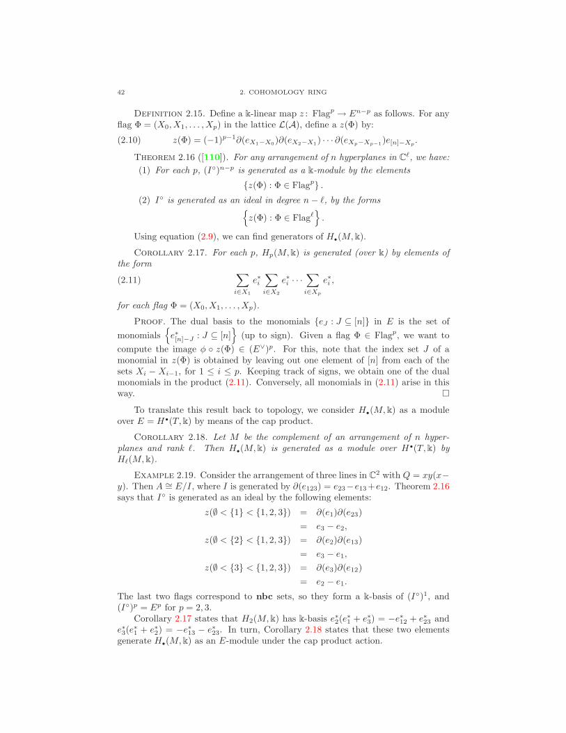
42 2. COHOMOLOGY RING
Definition 2.15. Define a k-linear map z : Flagp → En−p as follows. For anyflag Φ = (X0, X1, . . . , Xp) in the lattice L(A), define a z(Φ) by:
(2.10) z(Φ) = (−1)p−1∂(eX1−X0)∂(eX2−X1) · · · ∂(eXp−Xp−1)e[n]−Xp.
Theorem 2.16 ([110]). For any arrangement of n hyperplanes in Cℓ, we have:
(1) For each p, (I)n−p is generated as a k-module by the elements
z(Φ) : Φ ∈ Flagp .(2) I is generated as an ideal in degree n− ℓ, by the forms
z(Φ) : Φ ∈ Flagℓ
.
Using equation (2.9), we can find generators of H•(M, k).
Corollary 2.17. For each p, Hp(M, k) is generated (over k) by elements ofthe form
(2.11)∑
i∈X1
e∗i∑
i∈X2
e∗i · · ·∑
i∈Xp
e∗i ,
for each flag Φ = (X0, X1, . . . , Xp).
Proof. The dual basis to the monomials eJ : J ⊆ [n] in E is the set of
monomialse∗[n]−J : J ⊆ [n]
(up to sign). Given a flag Φ ∈ Flagp, we want to
compute the image φ z(Φ) ∈ (E∨)p. For this, note that the index set J of amonomial in z(Φ) is obtained by leaving out one element of [n] from each of thesets Xi − Xi−1, for 1 ≤ i ≤ p. Keeping track of signs, we obtain one of the dualmonomials in the product (2.11). Conversely, all monomials in (2.11) arise in thisway.
To translate this result back to topology, we consider H•(M, k) as a moduleover E = H•(T, k) by means of the cap product.
Corollary 2.18. Let M be the complement of an arrangement of n hyper-planes and rank ℓ. Then H•(M, k) is generated as a module over H•(T, k) byHℓ(M, k).
Example 2.19. Consider the arrangement of three lines in C2 with Q = xy(x−y). Then A ∼= E/I, where I is generated by ∂(e123) = e23−e13+e12. Theorem 2.16says that I is generated as an ideal by the following elements:
z(∅ < 1 < 1, 2, 3) = ∂(e1)∂(e23)
= e3 − e2,z(∅ < 2 < 1, 2, 3) = ∂(e2)∂(e13)
= e3 − e1,z(∅ < 3 < 1, 2, 3) = ∂(e3)∂(e12)
= e2 − e1.The last two flags correspond to nbc sets, so they form a k-basis of (I)1, and(I)p = Ep for p = 2, 3.
Corollary 2.17 states that H2(M, k) has k-basis e∗2(e∗1 + e∗3) = −e∗12 + e∗23 and
e∗3(e∗1 + e∗2) = −e∗13 − e∗23. In turn, Corollary 2.18 states that these two elements
generate H•(M, k) as an E-module under the cap product action.

2.4. HOMOLOGY AND VARCHENKO’S BILINEAR FORM 43
2.4.3. Homology II: the flag complex. In this section, we observe thatH•(M, k) can be described as a quotient of the vector space of all flags in L(A).(This turns out to be the Whitney homology of L(A), a fact we will not need here,and for which we refer to [242, 4.5]).
Theorem 2.20. For any arrangement of n hyperplanes in Cℓ, the kernel of thecomposition φ z : Flagp → (E∨)p is generated over k by all elements of the form
(2.12)∑
X:Xi−1<X<Xi+1
(X0, . . . , Xi−1, X,Xi+1, . . . , Xp),
for each flag Φ = (X0, X1, . . . , Xp).
Following [285], then, for each p define
(2.13) Flp = Flagp / ker(φ z),where the kernel is given by Theorem 2.20. Then, by construction, φ z induces anisomorphism
(2.14) Flp ∼= Hp(M, k),
for each p, 0 ≤ p ≤ ℓ.The homology of a (central) arrangement complement is a cochain complex in
a natural way.
Definition 2.21. Let δ∗ : (E∨)p → (E∨)p+1 denote the k-module homomor-phism given by δ∗(x) =
∑ni=1 e
∗i ∧ x.
Since E∨ is skew-commutative, clearly δ∗ δ∗ = 0, so δ∗ makes (E∨)∗ a cochaincomplex.
Proposition 2.22. The map δ∗ restricts to a cochain map on H•(M, k).
Proof. We have
(2.15)∑
i∈X1
e∗i · · ·∑
i∈Xp
e∗i
n∑
i=1
e∗i =∑
X∈Lp+1(A):Xp<X
∑
i∈X1
e∗i · · ·∑
i∈Xp
e∗i∑
i∈Xe∗i
Abusing notation, also let δ∗ denote the map δ∗ : Flagp → Flagp+1 obtainedfrom δ∗ above under the isomorphism (2.14). Via this identification, δ∗ : Flagp →Flagp+1 is given by
(2.16) δ∗(X0, . . . , Xp) =∑
X∈Lp+1(A):Xp<X
(X0, . . . , Xp, X).
It is easy to see, then, that relations (2.12) are sent to relations by δ∗, so δ∗ iswell-defined on Fl, hence on H•(M, k).
Proposition 2.23. For any central arrangement, we have (Fl, δ∗) ∼= (A, δ)∨,where −∨ denotes k-vector space duality, and δ is the chain map defined in Defini-tion 1.33.
Finally, H•(M, k) also has the structure of a chain complex, with a choice ofdifferential parameterized by elements of A1. Once again, it is best defined byidentifying H•(M, k) with a subcoalgebra of E∨.

44 2. COHOMOLOGY RING
Definition 2.24. For any element a ∈ H1(M, k), define a map ∂a : (E∨)p →(E∨)p−1 as follows. Write a =
∑ni=1 aiei. Let ∂a(e
∗i ) = ai, and extend ∂a to all of
E∨ by linearity and the Leibniz rule.
Proposition 2.25. For each a ∈ H1(M, k),
(1) The map ∂a induces a chain map on H•(M, k).(2) The isomorphism of graded k-vector spaces Fl ∼= A∨ induces an isomor-
phism of (co)chain complexes, (Fl, ∂a) ∼= (A, a)∨.
Proof. Given any a, the exterior algebra E = H•(T, k) is a cochain complexwith differential given by multiplication by the element a. The surjection of k-algebras E → A is therefore also a map of cochain complexes,
(2.17) (E, a)→ (A, a).
Now take the k-dual of the surjection (2.17). It is straightforward to check that(E, a)∨ = (E∨, ∂a). Since Fl = A∨, it follows that the differential ∂a restricts toFl, regarded as a subcomplex of (E∨, ∂a).
2.4.4. Definition of Sa. Now we are ready to define Varchenko and Schecht-man’s map S : H•(M, k) → H•(M, k). Using the algebra structure of E∨, weobserve:
Proposition 2.26. Any linear map s : V ∨ → V extends multiplicatively to aunique homomorphism of graded k-algebras s : E∨ → E, and by composition to amap S : H•(M, k)→ H•(M, k):
(2.18) H•(M, k)S //
i∗
H•(M, k)
H•(Tn, k)
s // H•(T n, k)
i∗
OO
We are interested in using this construction for certain choices of s.
Definition 2.27. let ∆: V ⊗k V → V be the diagonal homomorphism, and letǫ denote the canonical element in V ∨ ⊗k V . Let s = (1 ⊗∆)(ǫ), the image of ǫ inV ∨ ⊗ V ⊗ V . By adjunction, one may regard s as a k-linear map
s : V → Homk(V∨, V ).
Let M be the complement of a hyperplane arrangement. For any element a ∈H1(M, k), let Sa : H•(M, k) → H•(M, k) denote the map induced via Proposi-tion 2.26 from
s(a) : H1(M, k)→ H1(M, k).
The definition above makes sense for any cohomology ring generated in degree1. Using the distinguished basis for V , however, we may describe the maps Sa moreexplicitly. Let a =
∑Hi∈A aiei be any element of H1(M, k).
Lemma 2.28. The map Sa of Definition 2.27 is given in degree 1 by Sa(e∗i ) =
aiei for all i. Sa is given in degree p by extending this multiplicatively in E∨.
Proof. The first statement comes from following the natural isomorphisms.The second follows from Proposition 2.26.

2.4. HOMOLOGY AND VARCHENKO’S BILINEAR FORM 45
Equivalently, by adjunction, Sa may be indentified with a bilinear form onH•(M, k). To state this explicitly, define a bilinear form on E∨ by letting
(2.19) 〈e∗I , e∗J〉a =
ai1ai2 · · · aik if I = J ;
0 otherwise.
for monomials e∗I , e∗J ∈ E∨, where I = i1, . . . , ik. Then we observe the following:
Proposition 2.29. For all a ∈ H1(M, k) and Φ ∈ H•(M, k),
Sa(Φ) = 〈Φ,−〉a .That is, Sa : H•(M, k) → H•(M, k) is naturally identified with the restriction of〈, 〉a to H•(M, k).
Since the bilinear form 〈, 〉a on E∨ is symmetric, so is its restriction toH•(M, k).In other words,
Corollary 2.30. For any a ∈ H1(M, k), the map Sa is self-dual: Sa = S∨a .
Under the isomorphism (2.14), we may also understand Sa combinatorially asfollows. For Φ = (X0, X1, . . . , Xp) ∈ Flp,
(2.20) Sa(Φ) =∑
(i1,i2,...,ip)
ai1 · · · aipei1 · · · eip ,
where the sum is over all p-tuples for which λ(Hi1 , Hi2 , . . . , Hip) = Φ where, bydefinition, λ(Hi1 , Hi2 , . . . , Hip) is the flag
(0, Hi1 , Hi1 ∨Hi2 , Hi1 ∨Hi2 ∨Hi3 , . . . ,
p∨
j=1
Hij ).
2.4.5. Sa is a chain map. Recall from Proposition 2.25 that, for any a ∈ A1,the Orlik-Solomon complex (A, a) is k-dual to the chain complex (Fl, ∂a), whichappeared in Definition 2.24. If the arrangement is central, then furthermore (A, δ)is a chain complex dual to (Fl, δ∗), defined by Definition 2.21. The map Sa relatesthese two pairs of (co)chain complexes.
Proposition 2.31. For any central arrangement and any element a ∈ H1(M, k),
(1) Sa : (Fl, ∂a)→ (A, δ) is a map of chain complexes, and(2) Sa : (Fl, δ∗)→ (A, a) is a map of cochain complexes.
Proof. In view of Corollary 2.30, the isomorphisms (A, a) ∼= (Fl, ∂a)∨ and
(Fl, δ∗) ∼= (A, δ)∨, it is enough to prove (2) and then take k-duals. For this, thebilinear form point of view is convenient: one must check that
〈δ∗(Φ),Ψ〉a = 〈Φ, ∂a(Φ)〉afor all Φ,Ψ ∈ H•(M, k).
The bilinear form and differentials are all given by restriction from E∨ =H•(T, k), and the identity actually holds on E∨. That is, if I = i1, . . . , ik in-dexes a monomial e∗I , then
〈δe∗I , e∗J〉 = 〈e∗I , ∂a(e∗J)〉 = 0

46 2. COHOMOLOGY RING
unless J = i0 ∪ I for some i0 6∈ I. In that case,
〈δ∗(e∗I), e∗J〉 =⟨e∗i0e
∗I , e
∗i0e
∗I
⟩
= ai0ai1 · · · aik .Similarly, ∂a(e
∗J) = ai0e
∗I − e∗i0∂a(e∗I), from Definition 2.24, so
〈e∗I , ∂a(e∗J)〉 = 〈e∗I , ai0e∗I〉= ai0ai1 · · · aik
as well, which completes the proof.
2.4.6. Determinant formula. It turns out that if we take coefficients in afield, then Sa is an isomorphism of (co)chains on a Zariski open set in A1. Thisfollows from a remarkably explicit formula, due to Schechtman and Varchenko in[285], for the determinant of Sa in each degree. In order to state their result, let
(2.21) a(X) =∑
Hi≤Xai.
Also recall from (1.4.5) that, for a central arrangement A, the beta invariant β(A)is defined to be the Euler characteristic of the projective complement, and bi(A) =bi(M(A)), the ith betti number of the complement of A.
Theorem 2.32 ([285]). Let A be a rank-ℓ arrangement, and a ∈ A1. Then,for all p ≥ 0,
(2.22) detSpa = c∏
i≥0
∏
X∈Li(A)
a(X)β(AX)bp−i(AX),
where c is a nonzero scalar, depending on the choice of basis.
In particular, the following observation is immediate:
Corollary 2.33. The map Spa : Flp → Ap has full rank if and only if the suma(X) is nonzero for all subspaces X ∈ L≤p(A) for which AX is irreducible.
Example 2.34. Here we work out the braid arrangement A3 in detail. Theintersection lattice is drawn in Figure 1(b). Take the nbc-basis for A and its dualbasis for Fl. Let a =
∑1≤i<j≤4 aijeij be an element of A1. S1
a is just the diagonal
matrix with diagonal entries aij . If H is a hyperplane, M(AH) ∼= C∗, so theexponent in (2.22) for X = Hij is 1, and detS1
a =∏i<j aij .
For p = 2,
detS2a =
∏
1≤i<j<k≤4
(aij + aik + ajk)∏
1≤i<j≤4
a3ij ,
since for flats X of rank 2, β(AX) = 1 if X is a triple point and zero otherwise.For p = 3, we get
detS2a =
∑
1≤i<j≤4
aij
2∏
1≤i<j<k≤4
(aij + aik + ajk)∏
1≤i<j≤4
a2ij ,
since additionally for X = A3, we have β(AX) = β(A) = 2.

2.5. QUADRATIC OS ALGEBRA 47
2.5. Quadratic OS algebra
A graded associative algebra A is quadratic if it is generated by degree-oneelements and the kernel of the canonical map from the tensor algebra T (A1) toA is generated by elements of degree two. For example, exterior and symmetricalgebras are quadratic: the defining relations look like ab + ba and ab − ba, fora, b ∈ A1, respectively. Quadraticity is a necessary condition for an algebra to byKoszul; see Chapter 7. Because of the connection between the Koszul property andlower central series formulae (see it is natural to consider quadraticity of the Orlik-Solomon algebra. This property, which depends only on the underlying matroid,turns out to be exceedingly difficult to characterize combinatorially.
Definition 2.35. Let A be a graded, associative algebra generated in degree 1.Let I the kernel of the natural map T (A1)→ A, and let (Ik) be the ideal of T (A1)generated by the degree-k part of I. The quadratic closure of A is the quotient
A(2) = T (A1)/(I2).
The algebra A is quadratic if (I2) = I; that is, A(2) = A.
If A = A(A) for an arrangement A, then the quadratic closure A(2) is calledthe quadratic OS-algebra of A, written A(2)(A). Clearly, for A(A) to be quadraticit is sufficient that the OS ideal be generated by degree-two elements. If A(A) isquadratic, we will say that A is a quadratic arrangement.
Example 2.36. The rank-three braid arrangement is quadratic. Referring toExample 1.35, the OS-ideal is generated by four quadrics corresponding to the triplepoints, ∂e123, ∂e156, ∂e246, ∂e345, together with 3 degree-three relations of the form∂(epqrs), where Hp, Hq, Hr, Hs is a circuit. It suffices to show the cubic relationsare consequences of the quadrics. This is indeed the case: for example,
∂e2356) = (∂e23)e56 + e23(∂e56)
= (∂e23(∂e156 + e1∂e56) + e23(∂e56)
= (∂e23)(∂e156) + (e23 − e1(∂e23))∂e56= (∂e23)(∂e156) + (∂e123)(∂e56).
(2.23)
The remaining two cases are left as an exercise. This arrangement has the propertythat the minimal broken circuits for the given ordering all have size two. The com-putation above is intended to hint at the relevance of this property for quadraticity.In fact, this arrangement is one of a broad class of quadratic arrangements, the su-persolvable arrangements; see 3.4.6.
On the other hand, the arrangement with defining polynomial xyz(x+ y + z)is not quadratic: there are no 3-circuits, so I2 = 0, but I 6= 0. More generally, if Ais a k-generic arrangement (defined in Section 3.1) with 2 ≤ k < rk(A), then A isnot quadratic.
Quadratic arrangements were introduced in [118] (there called “2-determinedarrangements”) in connection with rational K(π, 1) arrangements. Some sufficientor necessary conditions for quadraticity were established early on. For example,here is a simple sufficient condition for quadraticity.
Definition 2.37. An arrangement A of rank three is parallel if, for any inde-pendent set of four hyperplanes in A, there is a fifth hyperplane H containing twoof the codimension-two intersections.
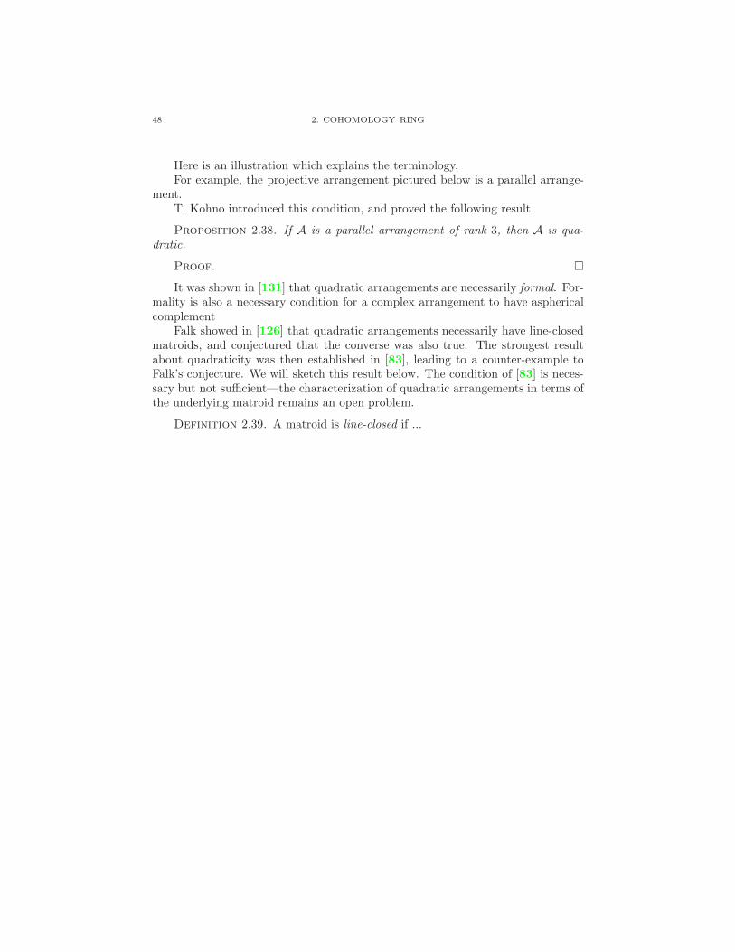
48 2. COHOMOLOGY RING
Here is an illustration which explains the terminology.For example, the projective arrangement pictured below is a parallel arrange-
ment.T. Kohno introduced this condition, and proved the following result.
Proposition 2.38. If A is a parallel arrangement of rank 3, then A is qua-dratic.
Proof.
It was shown in [131] that quadratic arrangements are necessarily formal. For-mality is also a necessary condition for a complex arrangement to have asphericalcomplement
Falk showed in [126] that quadratic arrangements necessarily have line-closedmatroids, and conjectured that the converse was also true. The strongest resultabout quadraticity was then established in [83], leading to a counter-example toFalk’s conjecture. We will sketch this result below. The condition of [83] is neces-sary but not sufficient—the characterization of quadratic arrangements in terms ofthe underlying matroid remains an open problem.
Definition 2.39. A matroid is line-closed if ...

CHAPTER 3
Special classes of arrangements
In this chapter we introduce several general classes of complex arrangementsthat have especially nice properties.
3.1. Generic arrangements
The simplest arrangement of all is the Boolean arrangement in Cℓ, consistingof the ℓ coordinate hyperplanes xi = 0, 1 ≤ i ≤ ℓ. The intersection lattice isisomorphic to the Boolean lattice of subsets of 1, . . . ℓ, ordered by inclusion. Thecomplement is the complex torus (C∗)ℓ. A generic arrangement is a generic sectionof a Boolean arrangement, a notion which we will now make precise.
Let A be an arrangement in Cℓ with intersection lattice L = L(A), and let Sbe a linear subspace of Cℓ not contained in any hyperplane of A. The arrangementH ∩ S | H ∈ A, S 6⊆ H in S is called the section of A by S. We denote thisarrangement by A ∩ S. Note that M(A ∩ S) = M ∩ S.
For example, it is easy to see that every essential central arrangement of nhyperplanes in Cℓ is isomorphic to an ℓ-dimensional section of the Boolean ar-rangement of n hyperplanes in Cn. Indeed, we can take S to be the image of themapping (α1, . . . , αn) : Cℓ → Cn, where α1, . . . , αn are the defining forms for A.(Compare Section 1.2.7.)
A section A ∩ S of A is called generic if X 6⊆ S for every X ∈ L \ 1L. Moregenerally, a section A ∩ S is generic in rank k if X 6⊆ S for every X ∈ L \ 1Lwith rk(X) ≤ k. Let L≤k = X ∈ L | rk(X) ≤ k. Then we immediately have thefollowing result.
Proposition 3.1. If A ∩ S is a section of A which is generic in rank k, thenL(A∩ S)≤k ∼= L≤k. In particular, if A ∩ S is a generic section of A by a subspace
S of dimension ℓ, then L(A∩ S) ∼= L≤ℓ−1 ∪ 1.
In terms of the projective point configuration A∗ dual to A, a codimension-onesection corresponds to projection of A∗ onto a hyperplane. This point of view isoften helpful. Consider, for example, the prism arrangement of rank four, whosematroid appears in Figure 1.5. The matroid of a generic rank-three section is justthe projection of this matroid onto the plane of the page.
By Proposition 3.1 the matroid of a generic hyperplane section of A dependsonly on the original matroid, and clearly this combinatorial operation can be definedat the level of matroids, realizable or not. This is called truncation: the truncationof a matroid M is obtained by adding a free point—one not contained in any circuitsexcept those of full rank—and then contracting on the new point. (This has the
effect of collapsing all flats of rank ≥ ℓ−1 to a single element 1.) Thus the matroidof a generic hyperplane section of A is the truncation of the matroid on A.
49

50 3. SPECIAL CLASSES OF ARRANGEMENTS
There are topological analogues of the preceding proposition, obtained fromthe Lefschetz hyperplane section theorem, proved in precise form by Hamm and Le[164].
Theorem 3.2. Suppose A∩ S is a generic section of A, with dim(S) = r + 1.Let ι : M ∩ S →M be the inclusion map. Then
(1) ι∗ : πi(M ∩S)→ πi(M) is an isomorphism for 1 ≤ i < r, and is surjectivefor k = r, and
(2) ι∗ : Hi(M) → Hi(M ∩ S)) is an isomorphism for 1 ≤ i < r, and isinjective for i = r.
The reader may consult [330] for a self-contained proof of Theorem 3.2 specificto hyperplane complements. As mentioned in Chapter 1.3, this theorem implies inparticular that π1(M(A)) ∼= π1(M(A′)) where A′ is a generic rank-three section ofA.
Definition 3.3. A generic arrangement of n hyperplanes in Cℓ is a genericsection of the Boolean arrangement in Cn by an ℓ-dimensional linear subspace.
A generic projective arrangement is by definition the projective image of ageneric central arrangement. Naturally, an affine arrangement is generic if andonly if its cone is generic. (In particular, in a generic affine arrangement no twohyperplanes are parallel.)
The truncated Boolean lattice of rank k is the collection of subsets of 1, . . . , nof cardinality at most k, together with the top element 1, . . . , n, ordered byinclusion. Recall E = En is the exterior algebra on e1, . . . , en.
Clearly any arrangement in C2 is generic. Did we do π1 for these guys?
Proposition 3.4. Let A be a generic arrangement of n hyperplanes in Cℓ,where ℓ > 2. Then
(1) L is isomorphic to the truncated Boolean lattice of rank ℓ.(2) π1(M) ∼= Zn, and πi(M) = 0 for 1 < i < ℓ.(3) Hp(M) ∼= Ep for 0 ≤ p < ℓ.
Proof. These statements follow from Proposition 3.1 and Theorem 3.2, andthe preceding remarks about the Boolean arrangement.
The underlying matroid of a generic arrangement of n hyperplanes in kℓ is bydefinition the uniform matroid Un,ℓ: a subset B of A is dependent if and only if|B| > ℓ.
Theorem 3.5. The homotopy type of the complement of a generic arrangementdepends only on the ambient dimension, ℓ, and the number of hyperplanes, n.
Proof. The realization space of the uniform matroid of rank ℓ on n points is aZariski-open subset of the Grassmannian of ℓ-planes in Cn, hence is path-connected.Then any two generic arrangements of n hyperplanes in Cℓ are lattice-isotopic. Theresult follows from Randell’s lattice-isotopy theorem [266].
Proposition 3.4 points toward a much stronger result, due to A. Hattori [169].Let T = S1. The n-torus T n has a standard minimal cell structure, defined asfollows. For I ⊆ 1, . . . , n let
T I = z ∈ T n | zi = 1 for i 6∈ I,

3.1. GENERIC ARRANGEMENTS 51
Figure 3.1. A generic affine arrangement of 3 lines
and let T nℓ =⋃
|I|=ℓ TI . Then T (i) is obtained by attaching
(ni
)i-cells to T (i−1).
Theorem 3.6. Let A be a generic projective arrangement of n+1 hyperplanesin CPℓ. Then M(A) is homotopy equivalent to T nℓ .
If n = ℓ, then A is the projective Boolean arrangement, with complement(C∗)n+1/C∗ ∼= (C∗)n ≃ T n.
Recent work of Randell [269], and Dimca–Papadima [93] generalizes a weakform of this theorem to arbitrary generic sections, as follows: if AS is an ℓ-dimensional generic section of a projective arrangement A, then M(AS) has thehomotopy type of the ℓ-skeleton of some minimal cell structure on M(A); see Sec-tion ??.
Hattori proves Theorem 3.6 by constructing an explicit homotopy equivalence.Rather than reproduce this argument, we refer the reader to [169], and instead givean informal treatment of the case ℓ = 2, n = 4. The argument can be formalizedusing the complexes of spaces and homotopy colimits; see [168, Section 4.G].
Suppose A is a generic projective arrangement of 4 hyperplanes in CP2. Thecomplement M(A) is diffeomorphic to the complement of a decone dA of A in C2,which, by Theorem 3.5, we may assume is given by x = 0, y = 0, x+ y = 2. WriteR2 as the union of three closed sectors U1∪U2∪U3, each containing one intersectionpoint, as in Figure 3.1.
Writing C2 = R2 × iR2, let Wi = (Ui × iR2) ∩ M(dA). Then M(dA) =W1 ∪W2 ∪W3. We claim that each Wi is homotopy equivalent to the 2-torus T 2.Note that, for (x, y) = (x1 + ix2, y1 + iy2) ∈ W1, we have x1 + y1 6= 2, so x+ y 6= 2.Thus W1 = (U1 × iR2) ∩M(B), where B is the Boolean arrangement consisting ofthe two lines x = 0, y = 0 through (0, 0). Then W1 is homotopy equivalent, byradial deformation, to (D2 × iR2) ∩M(B), which is a strong deformation retractof M(B). Since M(B) ∼= (C∗)2,, this shows that W1 is homotopy equivalent to the2-torus T 2. Similarly W2 and W3 are 2-tori, up to homotopy.
For i 6= j, Wi∩Wj is a copy of C∗, homotopy equivalent to S1, and the inclusionWi ∩Wj → Wi coincides, up to homotopy, with the inclusion S1 → T 2 = S1 × S1
onto one of the factors. Finally W1 ∩ W2 ∩ W3 is contractible. Then the unionM(dA) = W1∪W2 ∪W3 is homotopy equivalent to the union of three copies of T 2,
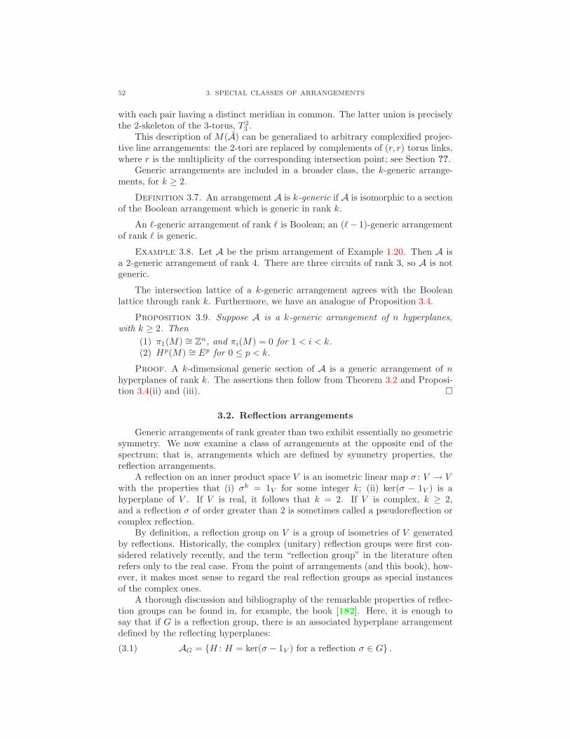
52 3. SPECIAL CLASSES OF ARRANGEMENTS
with each pair having a distinct meridian in common. The latter union is preciselythe 2-skeleton of the 3-torus, T 2
3 .This description of M(A) can be generalized to arbitrary complexified projec-
tive line arrangements: the 2-tori are replaced by complements of (r, r) torus links,where r is the multiplicity of the corresponding intersection point; see Section ??.
Generic arrangements are included in a broader class, the k-generic arrange-ments, for k ≥ 2.
Definition 3.7. An arrangement A is k-generic if A is isomorphic to a sectionof the Boolean arrangement which is generic in rank k.
An ℓ-generic arrangement of rank ℓ is Boolean; an (ℓ− 1)-generic arrangementof rank ℓ is generic.
Example 3.8. Let A be the prism arrangement of Example 1.20. Then A isa 2-generic arrangement of rank 4. There are three circuits of rank 3, so A is notgeneric.
The intersection lattice of a k-generic arrangement agrees with the Booleanlattice through rank k. Furthermore, we have an analogue of Proposition 3.4.
Proposition 3.9. Suppose A is a k-generic arrangement of n hyperplanes,with k ≥ 2. Then
(1) π1(M) ∼= Zn, and πi(M) = 0 for 1 < i < k.(2) Hp(M) ∼= Ep for 0 ≤ p < k.
Proof. A k-dimensional generic section of A is a generic arrangement of nhyperplanes of rank k. The assertions then follow from Theorem 3.2 and Proposi-tion 3.4(ii) and (iii).
3.2. Reflection arrangements
Generic arrangements of rank greater than two exhibit essentially no geometricsymmetry. We now examine a class of arrangements at the opposite end of thespectrum; that is, arrangements which are defined by symmetry properties, thereflection arrangements.
A reflection on an inner product space V is an isometric linear map σ : V → Vwith the properties that (i) σk = 1V for some integer k; (ii) ker(σ − 1V ) is ahyperplane of V . If V is real, it follows that k = 2. If V is complex, k ≥ 2,and a reflection σ of order greater than 2 is sometimes called a pseudoreflection orcomplex reflection.
By definition, a reflection group on V is a group of isometries of V generatedby reflections. Historically, the complex (unitary) reflection groups were first con-sidered relatively recently, and the term “reflection group” in the literature oftenrefers only to the real case. From the point of arrangements (and this book), how-ever, it makes most sense to regard the real reflection groups as special instancesof the complex ones.
A thorough discussion and bibliography of the remarkable properties of reflec-tion groups can be found in, for example, the book [182]. Here, it is enough tosay that if G is a reflection group, there is an associated hyperplane arrangementdefined by the reflecting hyperplanes:
(3.1) AG = H : H = ker(σ − 1V ) for a reflection σ ∈ G .

3.2. REFLECTION ARRANGEMENTS 53
It turns out, in particular, that AG is finite if and only if G is finite. AG is called areflection arrangement. An extensive treatment of such arrangements can be foundin [242, Chapter 6]; the reader should also see the subsequent paper of Broue,Malle, and Rouquier [29].
The importance of the arrangement to the group comes from the following.
Theorem 3.10. If G is a finite, real or complex reflection group, its reflectionaction permutes the hyperplanes AG. The induced action of G on MG = M(AG)is free.
On the other hand, the action of G on the projective complement M(A) is notfree: if a group element g ∈ G has an eigenvector v ∈ MG, then the image of vin P(V ) is fixed by g. Such eigenvectors are characterized via Springer’s theory ofregular elements, developed in [299].
To say G permutes the hyperplanes means G preserves the zero locus of thedefining polynomial Q(AG); however, the natural action of G on functions on Vdoes not fix the polynomial Q(AG). The discriminant of the reflection group G is aG-invariant polynomial of smallest degree whose zero locus is the union of reflectinghyperplanes.
Definition 3.11. The discriminant of G is the polynomial
δG =∏
H∈AG
αeH
H ,
where eH is the order of the subgroup of G that fixes H pointwise.
There is a close relationship between the invariant theory of reflection groupsand topology of the hyperplane complements, surveyed in [242, Chapter 6] and[29]. In particular, Orlik and Solomon proved the following:
Theorem 3.12 ([241]). If G is a (complex) reflection group, then
π(AG, t) =
ℓ∏
i=1
(1 + nit),
where the integers ni are the coexponents of the reflection group.
The coexponents of a reflection group will be defined in Chapter 9.A reflection group G is irreducible if and only if β(AG) 6= 0. The Shephard-
Todd classification of complex, irreducible reflection groups (see [39]) consists ofan infinite family G(r, p, ℓ), defined below, and 34 exceptional groups. The productdecomposition of an arrangement (1.4.5) takes the following form.
Theorem 3.13. If G is a reflection group, then there exist irreducible reflectiongroups G1, . . . , Gk, unique up to order, for which G = G1 × · · · × Gk. Moreover,AG = AG1 × · · · ×AGk
.
Accordingly, the irreducible reflection groups are of greatest interest.
Example 3.14 (Arrangements of types Aℓ, Bℓ, and Dℓ). For ℓ ≥ 1, the braidarrangement Aℓ of Example 1.8 is the product of the (irreducible) reflection ar-rangement of type Aℓ. The corresponding reflection group is the symmetric groupSℓ+1, which acts on Cℓ+1 by permuting the coordinates. (Technically, it is theessential arrangement in Cℓ+1/C ∼= Cℓ associated to Aℓ that has type Aℓ.)

54 3. SPECIAL CLASSES OF ARRANGEMENTS
The arrangements of type Dℓ and Bℓ, respectively, are defined by polynomials
δDℓ=
∏
1≤i<j≤ℓ(x2i − x2
j)2 and(3.2)
δBℓ= (x1x2 · · ·xℓ)2δDℓ
.(3.3)
The reflection group of type Bℓ is the hyperoctahedral group, defined geomet-
rically as the symmetry group of the vertices of the ℓ-cube, −1, 1ℓ in Rℓ. Thereflection group of type Dℓ is an index-2 subgroup, described explicitly in the nextexample.
The B3 arrangement (viewed from a corner of the cube) and its matroid isshown in Figure 3.2, with the hyperplanes in the order xyz(x−y)(x+y)(x−z)(x+z)(y − z)(y + z).
Example 3.15 (G(r, p, ℓ) arrangements). For r, p ∈ Z≥1 with p | r and ℓ ≥ 2,G(r, p, ℓ) is a group of order (rℓ/p)ℓ!. It is the semidirect product of the symmetricgroup Sℓ acting by permutations on the standard basis ei : 1 ≤ i ≤ ℓ, with thegroup of diagonal maps ei 7→ θiei, where θri = 1 and (θ1 · · · θℓ)q = 1 where q = r/p.The group acts irreducibly on Cℓ iff r > 1 and (r, p, ℓ) 6= (2, 2, 2).
G(r, 1, ℓ) = (Z/rZ)ℓ ⋊ Sℓ is called the full monomial group. All but four ex-ceptional, real reflection groups are members of this family: the Weyl groups oftype Aℓ−1, Bℓ, Dℓ, G2 and the dihedral groups I2(ℓ) equal respectively G(1, 1, ℓ),G(2, 1, ℓ), G(2, 2, ℓ), G(6, 6, 2), and G(ℓ, ℓ, 2). Their reflection action is given byrestricting the action above to Rℓ.
The discriminant of G(r, 1, ℓ) is
(3.4) δG = (x1x2 . . . xℓ)3
∏
1≤i<j≤ℓ(xri − xrj)2.
Its coexponents are ni = 1 + r(i − 1) for 1 ≤ i ≤ ℓ, so
π(AG, t) = (1 + t)(1 + (r + 1)t) · · · (1 + ((ℓ − 1)r + 1)t).
Figure 3.2. The B3-arrangement

3.4. SUPERSOLVABLE ARRANGEMENTS 55
3.3. Simplicial arrangements
3.4. Supersolvable arrangements
Some of the best understood arrangements are the supersolvable arrangements.Supersolvability is a purely combinatorial property of the intersection lattice. Itturns out that, in the case of complex arrangements, however, this property is justthe fiber-type property of §1.3.2 in disguise. We start by reviewing the relevantcombinatorics.
3.4.1. Modular flats.
Definition 3.16. Let L be a lattice. An element X ∈ L is modular if, forevery Y ∈ L,
(3.5) rk(X) + rk(Y ) = rk(X ∧ Y ) + rk(X ∨ Y ).
There are several equivalent formulations of modularity, see, for example, Lemma2.24 of [242]. A useful one here is the following: X is modular if, for all Z ∈ L andall Y ≤ Z,
(3.6) Y ∨ (X ∧ Z) = (Y ∨X) ∧ Z.This shows that there are isomorphisms between certain closed intervals in L,
for each modular element.
Lemma 3.17. X ∈ L is modular if and only if, for every Y ∈ L, the mapi : L → L, i(W ) = X ∧W gives an isomorphism [Y,X ∨ Y ] → [X ∧ Y,X ], withinverse j defined by j(W ) = Y ∨W .
Proof. If X is modular, then using (3.6) for Z ∈ [Y,X ∨ Y ],
ji(Z) = Y ∨ (X ∧ Z) = (Y ∨X) ∧ Z = Z,
where the last equality holds since Z ≤ X ∨ Y . Similarly, the composition ij is theidentity on [X∧Y,X ]. Conversely, for any Y ≤ Z, we have (X∨Y )∧Z ∈ [Y,X∨Y ],so
(X ∨ Y ) ∧ Z = ji(X ∨ Y ) ∧ Z) = Y ∨ (X ∧ (X ∨ Y ) ∧ Z) = Y ∨ (X ∧ Z).
By (3.6), X is modular.
For intersection lattices of arrangements, the modular property has a geometricreformulation: if A is a rank-ℓ arrangement, X is modular if, for all Y ∈ L(A), thesubspace X + Y ∈ L(A) as well. It easy to see that X ∈ L(A) is modular if itsrank is 0, 1, or ℓ. So all flats are modular for arrangements of rank ℓ < 3.
Example 3.18 (Rank 3). An arrangement of rank 3 can be viewed as a projec-tive line arrangement, where a flat of rank 2 is an intersection point. A point X ismodular if and only if it is joined to every other intersection point by a (projective)line in the arrangement. With this in mind, one can see from the picture that theB3-arrangement (Figure 3.2) has exactly three modular flats in codimension 2, thethree quadruple points. On the other hand, the X2 arrangement in Figure 3.4 hasno modular flats of rank 2. The reader may want to compare this with Example 1.31and Proposition 1.32.
Here are two results about inheriting the modular property that are useful forinduction arguments.

56 3. SPECIAL CLASSES OF ARRANGEMENTS
Lemma 3.19. Suppose X is a modular flat of an arrangement A.
(1) If H ∈ A and H 6≤ X, then X is modular in A \ H;(2) Z ∈ L(AX) is modular in AX if and only if Z is modular in A.
Proof. To prove the first statement, suppose there is some Y ∈ L(A \ H)for which X+Y 6∈ L(A\H). Since Y ∈ L(A) and X is modular, X+Y ∈ L(A).This means H ≤ X + Y , so H ≤ X , a contradiction.
The second statement is similar and appears in [242, Lemma 2.31].
3.4.2. Modular coatoms. To see that the modular property is interesting,it helps to restrict our attention to coatoms (that is, lattice elements of rank oneless than that of A.) If X is a modular coatom, one can learn quite a bit about Afrom AX . In particular, for such X and any hyperplane H 6≤ X , it must be thecase that X ∧H = V . So by Lemma 3.17,
(3.7) L(AH) ∼= L(AX).
Modular coatoms can be detected in codimension 2:
Lemma 3.20. If A is an arrangement of rank ℓ, then X ∈ Lℓ−1(A) is modularif and only if X + Y ∈ L(A) for all Y ∈ L2(A).
Proof. The one implication is immediate, so suppose a coatom X has theproperty that X + Y ∈ L(A) for all Y ∈ L2(A). Suppose Y ∈ Lk(A), and argueby induction on k. If Y ≤ X , then X + Y = Y , so it is enough to consider Y 6≤ Xand show X + Y ∈ Lk−1(A). The lattice is atomic, so
Y = H1 ∧H2 ∧ · · · ∧Hk
for some hyperplanes H1, . . . , Hk ∈ A. For arbitrary subspaces X,A,B, we alwayshave (X +A) ∩ (X +B) = X + (A ∩B), so
X + Y = (X +H1 ∩H2 ∩ · · · ∩Hk−1) ∩ (X +Hk−1 ∩Hk).
Since H1 ∩ H2 ∩ · · ·Hk−1 ∈ Lk−1(A) and Hk−1 ∩ Hk ∈ L2(A), by induction areboth X +H1 ∩ · · · ∩Hk−1 and X +Hk−1 ∩Hk. It follows that X + Y is in L(A)as well.
Theorem 3.21. If X is a modular coatom of an arrangement A, then
(3.8) π(A, t) = (1 +mt)π(AX , t),where m = |A| − |AX |.
Proof. We argue by induction on m, the number of H ∈ A for which H 6≤ X .Recall that a geometric lattice (§1.2.2) is atomic, so necessarily m ≥ 1. If m = 1,consider the deletion and restriction arrangements for the unique hyperplane Hfor which H 6≤ X . From our observation (3.7), the deletion and restriction areboth isomorphic to AX . So by the deletion-restriction recurrence (1.10), π(A, t) =(1 + t)π(A′, t).
If m ≥ 2, again L(A′′) ∼= L(AX). So by (1.10),
π(A, t) = π(A′, t) + tπ(AX , t)= (1 + (m− 1)t)π(AX , t) + tπ(AX , t)= (1 +mt)π(AX , t),
since by Lemma 3.19, X is modular in A′, and we may apply the induction hypoth-esis.
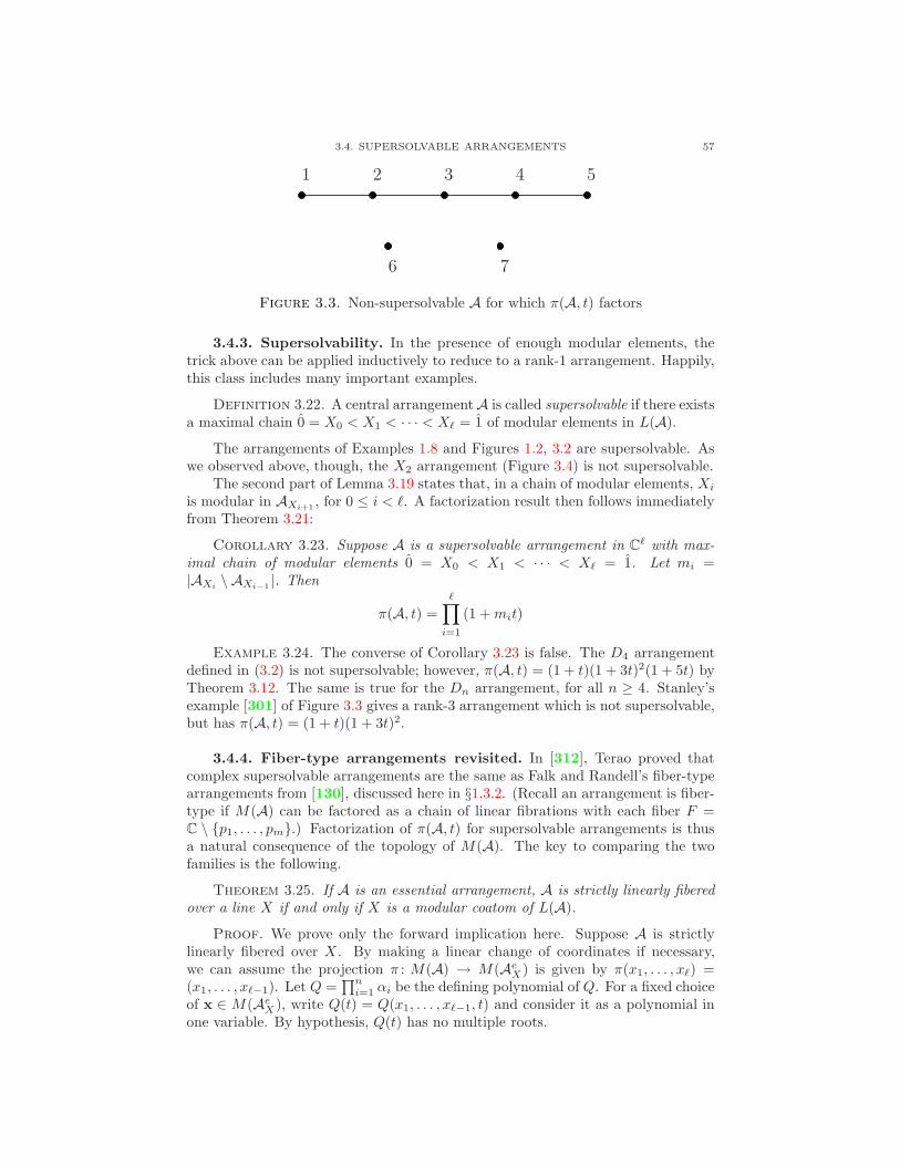
3.4. SUPERSOLVABLE ARRANGEMENTS 57
1 2 3 4 5
6 7
Figure 3.3. Non-supersolvable A for which π(A, t) factors
3.4.3. Supersolvability. In the presence of enough modular elements, thetrick above can be applied inductively to reduce to a rank-1 arrangement. Happily,this class includes many important examples.
Definition 3.22. A central arrangementA is called supersolvable if there existsa maximal chain 0 = X0 < X1 < · · · < Xℓ = 1 of modular elements in L(A).
The arrangements of Examples 1.8 and Figures 1.2, 3.2 are supersolvable. Aswe observed above, though, the X2 arrangement (Figure 3.4) is not supersolvable.
The second part of Lemma 3.19 states that, in a chain of modular elements, Xi
is modular in AXi+1 , for 0 ≤ i < ℓ. A factorization result then follows immediatelyfrom Theorem 3.21:
Corollary 3.23. Suppose A is a supersolvable arrangement in Cℓ with max-imal chain of modular elements 0 = X0 < X1 < · · · < Xℓ = 1. Let mi =|AXi
\ AXi−1 |. Then
π(A, t) =
ℓ∏
i=1
(1 +mit)
Example 3.24. The converse of Corollary 3.23 is false. The D4 arrangementdefined in (3.2) is not supersolvable; however, π(A, t) = (1 + t)(1 + 3t)2(1 + 5t) byTheorem 3.12. The same is true for the Dn arrangement, for all n ≥ 4. Stanley’sexample [301] of Figure 3.3 gives a rank-3 arrangement which is not supersolvable,but has π(A, t) = (1 + t)(1 + 3t)2.
3.4.4. Fiber-type arrangements revisited. In [312], Terao proved thatcomplex supersolvable arrangements are the same as Falk and Randell’s fiber-typearrangements from [130], discussed here in §1.3.2. (Recall an arrangement is fiber-type if M(A) can be factored as a chain of linear fibrations with each fiber F =C \ p1, . . . , pm.) Factorization of π(A, t) for supersolvable arrangements is thusa natural consequence of the topology of M(A). The key to comparing the twofamilies is the following.
Theorem 3.25. If A is an essential arrangement, A is strictly linearly fiberedover a line X if and only if X is a modular coatom of L(A).
Proof. We prove only the forward implication here. Suppose A is strictlylinearly fibered over X . By making a linear change of coordinates if necessary,we can assume the projection π : M(A) → M(AeX) is given by π(x1, . . . , xℓ) =(x1, . . . , xℓ−1). Let Q =
∏ni=1 αi be the defining polynomial of Q. For a fixed choice
of x ∈ M(AeX), write Q(t) = Q(x1, . . . , xℓ−1, t) and consider it as a polynomial inone variable. By hypothesis, Q(t) has no multiple roots.

58 3. SPECIAL CLASSES OF ARRANGEMENTS
Now Hi ≤ X if and only if the linear form αi does not depend on the variablet = xℓ, so we can write Q(t) = Q1 ·Q2(t), where
Q1 =∏
i : Hi≤Xαi(x) and Q2(t) =
∏
i : Hi 6≤Xαi(x, t),
and Q1 does not depend on t. The condition that Q(t) has no multiple roots meansthat, if αi(x, t) and αj(x, t) are proportional for some x ∈ Cℓ−1 (with i 6= j), thenQ1 vanishes. That is, there is a hyperplane H ≤ X for which (x, t) ∈ H , for allvalues of t.
But this is to say that (Hi ∩Hj) +X = H . Similarly, for each flat Y ∈ L2(A)with Y 6≤ X , then the hyperplane Y +X is contained in the arrangement A. ByLemma 3.20, X is modular.
Corollary 3.26. A complex arrangement A is supersolvable if and only if itis fiber-type.
Proof. Use induction on the rank of A, the rank 1-case being obvious. Ifℓ = rk(A) ≥ 2 and A is supersolvable, then it has a modular coatom Xℓ−1. ByTheorem 3.25, A is strictly linearly fibered overXℓ−1. Since AXℓ−1
is supersolvable,it is fiber-type, by induction, and A is too (Definition 1.26).
Similarly, if A is fiber-type, it is fibered over a modular coatom Xℓ−1, byTheorem 3.25. By definition, AeX is fiber-type, hence supersolvable. The modularelements in the chain X0 < X1 < · · · < Xℓ−1 are also modular in L(A), by
Lemma 3.19. Extending the chain by Xℓ = 1 shows A is supersolvable.
3.4.5. Cohomology rings. The combinatorial and topological characteriza-tions of supersolvability complement each other, as we see in particular when itcomes to the cohomology of M(A). For example, if A is strictly linearly fiberedover X , the E2-term of the Leray-Serre spectral sequence of the fibration
(3.9) Fm = C− m points // M(A)πX // M(AeX)
is Epq2 = Hp(M(AX), Hq(Fm,Z)). This is zero except for q = 0, 1, where Ep02 =
Hp(M(AX),Z) and Ep12 = Hp(M(AX),Zm). Falk and Randell [131] show that
the action of π1(M(AX)) on the cohomology of the fiber Fm is trivial, so Ep12∼=
Hp(M(AX)) ⊗ Zm. The existence of a section to πX implies that the spectralsequence collapses at E2. Since our spectral sequence converges to H•(M(A),Z),there is a short exact sequence for each p ≥ 1,
0 // Hp(M(AX),Z) // Hp(M(A),Z) // Hp−1(M(AX),Z)⊗Z Zm // 0.
Taken together, these short exact sequences say that, additively,
(3.10) 0 // A(AX) // A(A) // A(AX)(−1)⊗Z Zm // 0.
But the Leray-Serre spectral sequence is compatible with cup products, so (3.10)is actually a short exact sequence of A(AX)-modules.
Recall that, for any X ∈ L(A), the restriction πX : M(A) → M(AX) inducesa ring map π∗ : A(AX)→ A(A) so A(A) is a module over A(AX).
Proposition 3.27. If X is a coatom of A, then X is modular if and only ifA(A) is a free A(AX)-module.

3.4. SUPERSOLVABLE ARRANGEMENTS 59
Proof. If X is modular, then both ends of (3.10) are free A(AX)-modules,so A(A) is too. We leave the converse as an exercise. (Use Lemma 3.17 andCorollary 1.45.)
Note that, on the level of Betti numbers, the short exact sequence (3.10) impliesπ(A, t) = (1+mt)π(AX , t) (as in (3.8)), because π(A, t) is the Poincare polynomialof the algebra A(A). So, even though we saw in Example 3.24 that the factorizationof the Poincare polynomial does not imply supersolvability, a stronger statementon the level of algebras does.
Another way to formulate (3.10) is to let Tm denote the cohomology ring ofFm:
Tm = H•(Fm,Z)
= Z[e1, . . . , em]/(eiej : 1 ≤ i < j ≤ m),
a truncated (skew-commutative) polynomial ring with m generators. Then
(3.11) A(A) ∼= A(AX)⊗Z Tm
as A(AX)-modules. Missing from this formula is the algebra structure: this willappear in the Theorem below.
Bringing in the combinatorics of Orlik-Solomon algebras at this point makes amore complete understanding possible. Once again, the codimension-2 part of thelattice is in the spotlight. In view of Corollary 1.38, the next Lemma provides yetanother proof of the Poincare polynomial factorization (3.8). It is convenient tohave some additional notation.
Definition 3.28. Suppose X is a modular coatom of A. For any distincthyperplanes H and H ′ with H,H ′ 6≤ X , let H X H ′ = (H ∨H ′) ∧ X . It followsfrom the modularity of X that H X H ′ is a hyperplane of AX .
Proposition 3.29. Let X be a modular coatom of an arrangement A. If thehyperplanes of A are ordered so that hyperplanes AX come first, then
nbc(A) = nbc(AX) ∪⋃
H∈A−AX
S ∪ H : S ∈ nbc(AX) .
Proof. For brevity, let B = A \ AX . First note that, if H,H ′ ∈ B aredistinct, then H , H ′, and H X H ′ form a circuit. Since H X H ′ ∈ AX , bothH,H ′ ≻ H X H ′, so H,H ′ is a broken circuit.
So if S ∈ nbc(A), it contains at most one member of B. If S ∩ B = ∅, thenS ∈ nbc(AX), and conversely. If S ∩ B = H, let S′ = S − H. A fortiori, S′ isa nbc set for AX .
It remains to check that, if S ∈ nbc(AX), then H ∪ S ∈ nbc(A). If not,there would be a broken circuit A ∪ H with A ⊆ S. The corresponding circuitA∪H,H ′ would necessarily have H ′ ∈ AX , since H ′ is its least element, and thehyperplanes AX come first in order. Then A∪H ′ ⊆ AX , but since H 6∈ AX , theset A ∪ H,H ′ cannot be a circuit.
The last generalization of Theorem 3.21 is the following.
Theorem 3.30. Suppose that X is a modular coatom of an arrangement A.Then A(A) is a graded-commutative A(AX)-algebra, presented by
(3.12) A(A) ∼= A(AX)[eH : H ∈ A−AX ]/J,

60 3. SPECIAL CLASSES OF ARRANGEMENTS
where the generators eH are in degree 1 and the ideal J is generated by
(3.13) eHeH′ − (eH − eH′)eHXH′ ,
for all pairs H,H ′ ∈ A−AX .
Proof. Again, let B = A−AX , and define a A(AX)-algebra map
φ : A(AX)[eH : H ∈ B]→ A(A)
by letting φ(eH) = eH , for H ∈ B. Clearly φ is surjective, So we need to check thatthe relations (3.13) generate the kernel of φ. As we saw above, for eachH 6= H ′ ∈ B,the hyperplanes H,H ′, H X H ′ form a circuit and give the relation (3.13), soJ ⊆ ker(φ).
To see that J = ker(φ), recall that A(A) is a free A(AX)-module of rank m+1by Proposition 3.27, and so is A(AX)[eH : H ∈ B]/J .
3.4.6. Quadratic Grobner bases. As noted in Chapter 1, Bjorner showed in[23] that the monomials corresponding to broken circuits generate the initial idealof the Orlik-Solomon ideal I with respect to lex order, and in [25] Bjorner andZiegler showed that supersolvability is equivalent to the existence of an ordering forwhich the minimal broken circuits all have size two. Taken together, these resultsimply that if A is supersolvable, then there exists a quadratic Grobner basis forI(A).
In [256] Peeva showed that the converse holds. To see this, note that if ≺ isany monomial order in which e1 ≻ e2 ≻ · · · ≻ en, and ≺lex is the lex order whichorders the variables in the same way, then
(3.14) in≺ I = in≺lexI.
To see this, note that for a circuit m, ∂(m) consists of monomials which (pairwise)differ in a single entry. For a pair of such monomials, p ∧ ei ≺ p ∧ ej if and only ifp ∧ ei ≺lex p ∧ ej . Thus,
in≺(∂(m)) = in≺lex(∂(m))
By Bjorner’s result, in≺lex(I) = 〈b | b a broken circuit〉, and combining this with
the previous observation shows that
in≺lex(I) ⊆ in≺(I).
If the containment were proper, then in≺(I) would of necessity contain a monomialcorresponding to a non-broken circuit p. If deg(p) = i, then
dimk (E/ in≺(I))i 6= dimk (E/ in≺lex(I))i ,
contradicting the fact that passing to initial ideals preserves the Poincare series.Hence, equality (3.14) holds, and this yields:
Theorem 3.31. I(A) has a quadratic Grobner basis iff A is supersolvable.
This algebraic characterization of supersolvability highlights one special prop-erty of Orlik–Solomon ideals. Any monomial order must order the variables, andin the case of the Orlik–Solomon ideal, the initial ideal that results is the same asthat obtained using the lex order. In particular, this determines all possible initialideals of I. For an arbitrary ideal, this is typically an involved process, but forOrlik–Solomon ideals it is simple.

3.5. HYPERSOLVABLE ARRANGEMENTS 61
One important consequence of the existence of a quadratic Grobner basis forthe Orlik–Solomon algebra A is the fact that this implies A is Koszul. This wasshown by Froberg, see his survey [149] for more information. As we shall see inChapter 5, the Koszul property has important topological consequences. Althoughthe existence of a quadratic Grobner basis for a k–algebra implies the algebra isKoszul, it is not necessary. In [111] Eisenbud-Reeves-Totaro show that if k is aninfinite field and I is generated by e generic quadratic forms in k[x1, . . . , xe+n], withe, n ≥ 0, then if 3n <
(e−12
), the ideal I does not admit a quadratic Grobner basis.
Open Problem 3.32. Let A be an arrangement, with Orlik–Solomon algebraA = E/I. Does A Koszul imply that I has a quadratic Grobner basis (hence, thatA is supersolvable)?
Example 3.33 (X2 arrangement). It is easy to find examples of arrangementswhere I is minimally generated by quadrics, but does not have a quadratic Grobnerbasis. The following arrangement in C3 was first studied by Kohno; the definingpolynomial is Q = xyz(x+ y)(x− z)(y − z)(x+ y − 2z) and
π(A, t) = (1 + t)(1 + 6t+ 10t2)
1
2
3
4
56
24
5
1 6
0
3
Figure 3.4. Intersection with a two-plane, and matroid of A
The intersection of A with the two-plane determined by z = 1 as well as thematroid of A are shown in Figure 3.4. For this example, it can be checked that Ais not Koszul.
3.5. Hypersolvable arrangements
The class of supersolvable arrangements has a natural generalization to hyper-solvable arrangements. Let A = H1, . . . , Hn be a central arrangement in thecomplex vector space V . Denote also by A = a1, . . . , an ⊂ P(V ∗) its set ofdefining equations, viewed as points in the dual projective space. Let B ⊂ A be aproper, non-empty sub-arrangement, and set B := A \ B. We say that (A,B) is asolvable extension if the following conditions are satisfied.
(I) No point a ∈ B sits on a projective line determined by α, β ∈ B.(II) For every a, b ∈ B, a 6= b, there exists a point α ∈ B on the line passing
through a and b. (In the presence of condition (I), this point is uniquelydetermined, and will be denoted by f(a, b).)
(III) For every distinct points a, b, c ∈ B, the three points f(a, b), f(a, c), andf(b, c) are either equal or collinear.

62 3. SPECIAL CLASSES OF ARRANGEMENTS
α
β
6 ∃ a
(I)
a
b
∃!f(a, b)
(II)
a
b
c
f(a, b)
f(a, c)
f(b, c)
(III)
Figure 3.5. Axioms for solvable extensions
Note that only two possibilities may occur: either rk(A) = rk(B) + 1 (fiberedcase), or rk(A) = rk(B) (singular case).
Definition 3.34 ([176]). The arrangement A is called hypersolvable if it hasa hypersolvable composition series, i.e., an ascending chain of sub-arrangements,A1 ⊂ · · · ⊂ Ai ⊂ Ai+1 ⊂ · · · ⊂ Aℓ = A, where rkA1 = 1, and each extension(Ai+1,Ai) is solvable.
The length of a composition series depends only on A; it will be denoted byℓ(A). Note that the property of being hypersolvable is purely combinatorial. Infact, given an arrangementA, one can decide whether it is hypersolvable or not, onlyfrom the elements of rank one and two of L(A), since the definitions only involvethe collinearity relations in A. The class of hypersolvable arrangements includessupersolvable arrangements, cones of generic arrangements (for which ℓ(A) = |A|),and many others.
We may assume, whenever necessary, that a given hypersolvable arrangement isalso essential. Indeed, one knows how to associate to an arbitrary central arrange-ment A an essential arrangement, Aess, without changing the homotopy types ofthe complements, X(A) and X ′(A), and the intersection lattice L(A).
The connection between hypersolvable and supersolvable (or fiber-type) ar-rangements comes from the following fact. If the solvable extension (A,B) is fibered,then there is a Serre fibration X(A)→ X(B), with homotopy fiber C \ m points,where m = |B|. The (topological) definition of fiber-type arrangements may berephrased in hypersolvable terms, as follows.
Definition 3.35. The arrangement A is supersolvable (or, fiber-type) if it hasa supersolvable composition series, that is, a hypersolvable composition series as inDefinition 3.34, for which all extensions are fibered.
We thus see that all fiber-type arrangements are hypersolvable. On the otherhand, if (A,B) is a solvable extension that is not fibered, then there is a fibered
extension (A,B) such that A is a hyperplane section of A; see [176]. This implies,for instance, that a hypersolvable arrangement A is aspherical if and only if A isfiber-type, which happens precisely when ℓ(A) = rk(A); again, see [176].
3.6. Graphic arrangements
Let Γ be a graph, with vertex set [ℓ] = 1, . . . , ℓ, and edge-set E. We shallassume Γ is a simple graph, that is, there are no loops or multiple edges.

3.6. GRAPHIC ARRANGEMENTS 63
Definition 3.36. The graphic arrangement associated to Γ is the followingarrangement of hyperplanes in Cℓ:
AΓ = zi − zj = 0 | (i, j) ∈ E.If Γ = Kℓ is the complete graph on ℓ vertices, then clearly AΓ is the Braid
arrangement Aℓ−1 defined in Example 1.8. There are often pleasing connectionsbetween invariants of Γ and invariants of AΓ, which we now describe.
A coloring of a graph Γ with n colors is an assignment of an integer in 1, . . . , nto each vertex of Γ, such that no two adjacent vertices share the same number. Thechromatic function χ(Γ, n) is the number of colorings of Γ with n colors.
Definition 3.37. Fix an edge i, j of Γ. The deletion Γ′ = Γ \ i, j, and thecontraction Γ′′ is obtained by identifying vertex i and j.
Clearly Γ′ has the same set of vertices as Γ, but one less edge, while Γ′′ has oneless vertex than Γ, and at least one less edge than Γ. In particular, Γ′′ may not bea simple graph.
Lemma 3.38. For (Γ,Γ′,Γ′′) as above, χ(Γ′, t) = χ(Γ, t) + χ(Γ′′, t).
Proof. A coloring of Γ clearly gives a coloring of Γ′, so there is an inclusionof sets colorings of Γ ⊂ colorings of Γ′. The complement of this set inclusionconsists of colorings of Γ′ which have the same color assigned at vertices i and j;such colorings correspond to colorings of Γ′′.
Recall that under the operation of deletion–restriction, the Poincare polynomialsatisfies the relation π(A, t) = π(A′, t) + tπ(A′′, t). Combining this relation andEquation ?? shows that the characteristic polynomial satisfies:
χ(A′, t) = χ(A, t) + χ(A′′, t)
Applying deletion-restriction to a graphic arrangement, with H the hyperplaneassociated to edge i, j, we have
χ(AΓ′ , t) = χ(AΓ, t) + χ(AΓ′′ , t)
In sum, the characteristic polynomial of a graphic arrangement satisfies the sameidentity as the chromatic polynomial, and an inductive argument proves:
Proposition 3.39. If AΓ is a graphic arrangement, then χ(AΓ, t) = χ(Γ, t).
An induced subgraph of Γ is a subgraph obtained by specifying a subset S ofthe vertices of Γ, and deleting all edges with vertices outside of S. An induced cycleof Γ is an induced subgraph which is a cycle. The induced cycles of Γ appear inthe cohomology ring of M(AΓ) in a very natural way:
Lemma 3.40 ([289]). Let AΓ be the arrangement corresponding to a graph Γ.If we write aj for the number of minimal generators of degree j of I(AΓ), then, forall j > 2,
(3.15) aj = #chordless (j + 1)-cycles of Γ.Proof. Chordless m-cycles are circuits, and give rise to degree m−1 elements
of the Orlik-Solomon ideal. The correspondence is one-to-one because a circuite1, . . . , em gives a relation
∑
i
(−1)ie1 · · · ei · · · em.

64 3. SPECIAL CLASSES OF ARRANGEMENTS
•
•
•???
????
????
•
•
??????????
Figure 3.6. A non-hypersolvable graph
The lead monomial of some lower degree element of I divides e1 · · · em−1 if and onlyif that monomial corresponds to a chord of 1, . . . ,m, contradicting the fact that1, . . . ,m is a circuit.
Example 3.41. Let Γ be the one-skeleton of the Egyptian pyramid, shown inFigure 3.6. The arrangement AΓ is the simplest example (in terms of number ofvertices) of a graphic arrangement which is not hypersolvable. By Lemma 3.40,the Orlik-Solomon ideal has four quadratic generators, and one cubic generator,corresponding to the base of the pyramid. Using Proposition 3.39 and Deletion-Contraction, we compute that π(AΓ, t) = 1 + 8t+ 24t2 + 31t3 + 14t4.
Combining Lemma 3.40 with Theorem 3.31 shows that a necessary conditionfor supersolvability of AΓ is that Γ be chordal: the minimal induced cycles aretriangles. In fact, this is both necessary and sufficient.
Theorem 3.42 (Stanley [301]). The arrangement AΓ is supersolvable if andonly if the graph Γ is chordal.
Combining this with Theorem 3.31 solves Problem 3.32 in the graphic case: AΓ
is Koszul exactly when AΓ is supersolvable.Will LCS ranks be on table yet We close by mentioning that for graphic
arrangements, the connection between the fundamental group and the cohomologyring is very close. For example, Kohno proved in [195] that the LCS ranks of thebraid arrangement An−1 are given by:
(3.16)∞∏
k=1
(1− tk)φk = π(An−1,−t) =n−1∏
i=1
(1− it),
This will be explored in great detail in Chapter 6.

CHAPTER 4
Resonance varieties
We return to the Orlik-Solomon algebra of an arrangement A, focusing nowon the ring structure. We construct and analyze certain algebraic invariants of thegraded ring A = A(A), called resonance varieties, which will play a central rolethroughout the remainder of the book.
The resonance varieties were defined in [124], where they were used by Falkto distinguish the ring structure of OS-algebras of arrangements for which manyother invariants (e.g., characteristic and Tutte polynomials) coincide. Now the mainmotivation for the study of resonance varieties comes from the tangent cone formula(Section 10.1), which relates the degree-one resonance varieties to the characteristicvarieties of π1(M(A)).
The description of degree-one resonance varieties leads to some interesting andintricate combinatorics, geometry, and homological algebra. The combinatorial andgeometric aspects of resonance varieties will be the topic of this chapter; algebraicaspects will be taken up in Chapter 7. Higher degree resonance varieties are a topicof current research—we will sketch some of what is currently known.
4.1. The cochain complex determined by a one-form
4.1.1. The resonance varieties of a graded algebra. Let k be a field.Suppose A is a graded, graded-commutative, connected k-algebra of finite type,satisfying a2 = 0 for a ∈ A1. (This is automatic unless k has characteristic two.)For an element a ∈ A1, consider the map A→ A given by x 7→ ax. This is a gradedhomomorphism of degree one, and squares to zero, so we have a cochain complex
(4.1) A0 a // A1 a // · · · a // Ara // · · ·
We denote this complex by (A, a), and its cohomology by H∗(A, a).
Definition 4.1. Let p ≥ 0. The degree-p resonance variety of A is the set
Rp(A) =a ∈ A1 | Hp(A, a) 6= 0
.
The set Rp(A) is filtered by the dimension of Hp(A, a). That is, Rp(A) =Rp1(A) is the largest of the decreasing sequence of subsets
(4.2) Rpk(A) = a ∈ A1 | dimHp(A, a) ≥ k,defined for all k ≥ 1. If bp = dimk A
p denotes the p-th Betti number of A, we havefor every p ≥ 0 a filtration
(4.3) A1 ⊇ Rp1(A) ⊇ · · · ⊇ Rpbp(A) ⊇ Ribp+1(A) = ∅.
Evidently, if Ap = 0, then Rpk(A) = ∅, for all k ≥ 1. In degree 0, things are verysimple: R0
1(A) = 0, while R0k(A) = ∅, for k > 1.
65

66 4. RESONANCE VARIETIES
It is easy to check that Rpk(A) is a Zariski closed subset of the affine space
A1 ∼= kb1 . Indeed,Rpk(A) is defined by the vavishing minors of matrices representingthe multiplication maps a : Ap−1 → Ap and a : Ap → Ap+1. The entries of thesematrices are linear in a, so Rpk(A) is a determinantal variety.
Clearly, H∗(A, a) = H∗(A, ca), for all c ∈ k\0. Thus, each resonance varietyRp(A) is homogeneous. The projective image of Rp(A) in P(A1) is called the p-thprojective resonance variety of A, and is denoted by Rp(A); likewise for Rpk(A).
4.1.2. Resonance varieties of arrangements. Now let A = H1, . . . , Hnbe a central arrangement of rank ℓ, and let A = H∗(M(A), k) be the OS-algebraof A over k. Since H∗(M(A),Z) is torsion-free, we have a2 = 0 for all a ∈ A1, byuniversal coefficients. Thus, the resonance varieties of the OS-algebra, Rpk(A), aredefined even if chark = 2.
The study of the cohomology groups H∗(A, a) was initially motivated by theresults of [115, 284] relating H∗(A(A), a) to the cohomology of the rank-one localsystem on the complement M(A) associated with a (see Theorem 8.17). In theremainder of this section we prove some general “non-resonance” results concerningH∗(A, a), culminating in a vanishing theorem of Yuzvinsky [338] (Theorem 4.6).These results give necessary conditions for an element a ∈ A1 to lie in Rp(A), forp < rk(A) − 1.
The natural basis for A1 will be denoted by e1, . . . , en. For a ∈ A1, we writea =
∑ni=1 aiei. Recall the map ∂ : A→ A of Section 1.4.4, defined by ∂(ei) = 1 for
1 ≤ i ≤ n, and ∂(ab) = (∂a)b+ (−1)deg(a)a(∂b) for a, b ∈ A.
Proposition 4.2. If a ∈ A1 and ∂a 6= 0, then H∗(A, a) = 0.
Proof. Let c = ∂a ∈ k − 0. As a straightforward check shows, c−1∂ is achain homotopy between the identity and the zero maps of the cochain complex(A, a). Hence the complex is exact.
Let A be the projectivization of A. The projective OS-algebra A(A) is thekernel of ∂, a subalgebra of A. We denote A(A) by A.
If a ∈ A1 satisfies ∂a = 0, then a ∈ A1, so by restriction we have a complex(A, a).
Proposition 4.3. If a ∈ A1 with ∂a = 0, then there is a split short exactsequence of graded k-vector spaces,
0 // H∗(A, a) // H∗(A, a) // H∗(A, a)[−1] // 0 .
In particular, for each p ≥ 0,
Hp(A, a) ∼= Hp(A, a)⊕Hp−1(A, a)
Proof. Under the hypothesis that ∂a = 0, the short exact sequence of Theo-rem 1.47(ii) is actually a short exact sequence of cochain complexes,
0 // (A, a) // (A, a)∂ // (A[−1],−a) // 0 .
Moreover, the splitting map s : A[−1] → A defined by s(x) = enx gives rise to a(degree zero) map of cochain complexes, s : (A[−1],−a) → (A, a). It follows thatthe long exact sequence in cohomology splits into split short exact sequences, asclaimed.

4.1. THE COCHAIN COMPLEX DETERMINED BY A ONE-FORM 67
Recall from Section 1.4.5 that the Euler characteristic χ(M(A)) coincides (upto sign) with the beta invariant β(A), see (1.29); for complexified arrangements, thisis the number of bounded chambers of the underlying real arrangement. As is well-known, a cochain complex and its cohomology have the same Euler characteristic,see e.g. [168, Thm. 2.44]. In our setting, this implies the following equality.
Proposition 4.4. Suppose a ∈ A1. Then
ℓ−1∑
i=0
(−1)i dimHi(A, a) = χ(M(A)) = (−1)rk(A)−1β(A).
Example 4.5. Let A be a generic central arrangement of n hyperplanes in Cℓ.Let E =
∧(A1). Then dim(E1) = n − 1, and A ∼= E/(Eℓ). This follows from the
presentation 1.4.4 obtained by specifying a hyperplane at infinity. Then
(4.4) χ(M(A)) = χ(E/(Eℓ)) =ℓ−1∑
p=0
(−1)p(n− 1
p
).
(This is the number of bounded chambers in a generic arrangement of n− 1 affinehyperplanes in Rℓ−1, up to sign.)
Any nonzero element a ∈ A1 can be included in a basis of A1. Since Ap = Ep forp < ℓ−1, it follows that Hp(A, a) = 0 for p < ℓ−1. Then Hℓ−1(A(A, a)) ∼= kβ(A).By Proposition 4.3, Hp(A, a) vanishes for 0 ≤ p < ℓ−1, and is isomorphic to kβ(A)
for p = ℓ− 1, ℓ.
The preceding example was generalized to arbitrary arrangements in [338].For a general central arrangementA of rank ℓ, the cohomology groups Hp(A(A), a)vanish for p < ℓ−1, provided a satisfies some numerical conditions we specify below.This yields necessary conditions for Hp(A(A), a) to be nonzero for p < ℓ − 1, inwhich case we say the element a ∈ A1 is resonant.
4.1.3. Yuzvinsky’s vanishing theorem. A proof of the vanishing theorembelow appears in the book [244], using a different approach. We will reproducethe original argument of [338]. The sheaf of OS-algebras on the finite poset L0
used in the proof ought to be more generally applicable, while at the same time theargument gives nice, simple examples of computations of sheaf cohomology. Werefer to [20] for generalities about sheaves on posets.
Let L = L(A) be the intersection lattice. For X ∈ L, let AX denote the lo-calization of A at X , and let AX = A(AX). There is then a canonical surjectionA ։ AX , corresponding to the inclusion of spaces M(A) ⊆ M(AX)—see Theo-rem 2.4. For an element a ∈ A1, denote by aX its image in AX .
Let L0 = L(dA) = X ∈ L | X 6≥ Hn be the intersection semi-lattice of thedecone of A relative to Hn; for the purpose of using sheaves, we order L0 byinclusion. In particular, L0 has always a largest element, namely, Hn. We use thenotion of rank from L, but notice that rank becomes a decreasing function on L0.
Recall from Theorem 1.54 the affine Brieskorn decomposition
(4.5) Ap ∼=⊕
X∈L0
rk(X)=p
ApX .
Let us say X is irreducible if AX is an irreducible arrangement (Section 1.4.5).Note that each hyperplane H ∈ A is irreducible.

68 4. RESONANCE VARIETIES
Theorem 4.6. Suppose a ∈ A1 and ∂(aX) 6= 0 for every irreducible X ∈ L0.Then
(i) Hp(A, a) = 0, for p < ℓ− 1.(ii) Hp(A, a) = 0, for p < ℓ− 1.(iii) Hℓ−1(A, a) ∼= Cβ(A).(iv) Hℓ−1(A, a) ∼= Hℓ(A, a) ∼= Cβ(A).
Proof. The last three statements follow from the first, by Propositions 4.4and 4.3. The first statement is proved by induction on rk(A). If rk(A) is one ortwo, then A is generic, and the result holds by Example 4.5. Assume (i)– (iv) holdfor all arrangements of rank less than ℓ. We define a complex of sheaves Y with L0
as the underlying topological space. An open set in L0 is an increasing set, that is,a set U with the property X ∈ U and Y ≥ X implies Y ∈ U . Let UX = L(AX);these sets form a basis for the topology. We set Γ(UX ,Yp) = ApX . Using 4.5, wesee that there is a projection ρpXY : ApX → ApY whenever UX ⊇ UY . Set ρpXY = 0 ifrk(Y ) 6= p. This defines a presheaf Yp on L0 for each p. By (4.5),
(4.6) Γ(U,Y) ∼=⊕
X∈Urk(X)=p
ApX .
The sheaf axioms follow. Moreover, each Yp is flasque: any element of Γ(U,Yp) isthe restriction of an element of Γ(L,Yp). The space of global sections Γ(L0,Yp) isisomorphic to Ap.
Multiplication by aX defines a homomorphism Γ(UX ,Yp) → Γ(UX ,Yp+1).These homomorphisms define a complex of sheaves
(4.7) Y0 // Y1 // · · · // Yℓ // 0 .
Restricting to the stalk at X we get a cochain complex,
(4.8) 0 // A0X
// A1X
// · · · // ApX// 0 ,
where p = rk(X). Since 1 6∈ L0, p < ℓ. Then the inductive hypothesis ensuresthat the latter complex is acyclic, as follows. If ∂aX 6= 0, and H∗(A(AX ), aX) = 0by Proposition 4.2. If ∂aX = 0, then X is reducible, so β(AX) = 0 by Proposi-tion 1.57. The inductive hypothesis implies Hq(A(AX), aX) = 0, for q < p−1, andHp−1(A(AX), aX) ∼= Hp(A(AX ), aX) ∼= Cβ(AX) = 0 as well.
Thus 4.7 defines a flasque resolution of the kernel E of the 0th differentialY0 → Y1. E is a skyscraper sheaf, more precisely, it has the only nonzero stalk atthe largest element of L0, and this stalk is C. Then the complex of global sections
(4.9) Γ(L0,Y0) // Γ(L0,Y1) // · · · // Γ(L0,Yℓ−1) // 0 ,
computes the cohomology of the base space L0, with coefficients in E . But thecomplex of global sections is just the OS algebra complex
(4.10) A0 a // A1 a // · · · a // Aℓ−1 .
The proof is completed by showing Hp(L0, E) = 0 for p < ℓ − 1. This goesas follows. First use the exact cohomology sequence arising from the short exactsequence of sheaves
(4.11) 0 // E // K // K0// 0 ,

4.2. DEGREE-ONE RESONANCE VARIETIES 69
where K denotes the constant sheaf on L0, and K0 its restriction to L0 \ Hn.The cohomology H∗(L0,K) is the cohomology of the order complex |L0| of Defi-nition 1.13. The latter complex is contractible because L0 has a largest element.Then Hp(L0, E) ∼= Hp−1(L0,K0). Finally since L0 \ Hn is an open interval in ageometric lattice we have Hp−1(L0 \ Hn,K0) = 0 for p < ℓ − 1 by the Folkmantheorem (see [145]).
As an immediate corollary we obtain an extension of Example 4.5 to “almostgeneric” arrangements.
Corollary 4.7. Suppose there is a hyperplane Hi ∈ A such that the ar-rangement A \ Hi is generic. Let a ∈ A1 with with aj 6= 0 for j 6= i. ThenHp(A, a) = Hp(A, a) = 0 for 0 ≤ p < ℓ− 1.
Theorem 4.6 can be restated in terms of resonance varieties. If we set KX =a ∈ A1 | ∂(aX) = 0, the theorem states that Rp(A) is contained in the union ofthe KX for X ∈ L0 with β(AX) 6= 0, for p < rk(A) − 1.
4.2. Degree-one resonance varieties
Let A = H1, . . . , Hn be a central arrangement, and A = Ak(A) the OS-algebra of A over a field k. In this section we give a simple description of thedegree-one resonance variety R1(A). For notational convenience, we denote thisvariety by R(A).
There is a decomposition RΓ(A) of R(A) parametrized by certain partitionsΓ of subarrangements of A. Each of these partitions Γ determines a linear subspaceKΓ of A, andRΓ(A) is a subvariety of KΓ. The projective image RΓ(A) is naturallyruled by lines, with the ruling determined in a simple way by Γ.
In the next section we will specialize further, assuming k has characteristiczero. In this case, the varieties RΓ(A) are linear and intersect trivially. In fact,there is only one known example, over any field, for which R(A) is not a union oflinear subspaces—we exhibit that example at the end of this section.
4.2.1. Resonant pairs. Let a ∈ A1. Observe that a ∈ R(A) if and only ifthere exists b ∈ A1 not proportional to a such that ab = 0. If this is the case, thenb ∈ R(A) also. It is this symmetry that makes the case p = 1 special. In fact,the entire plane spanned by a and b lies in R(A); this is where the ruling of R(A)comes from. In this situation we call the pair (a, b) a resonant pair.
The first step is to treat the rank-two case. Recall A1 = A1(A) = a ∈ A1 |∑ni=1 ai = 0.
Theorem 4.8. Suppose A has rank two. Then R(A) = A1 if |A| ≥ 3, andR(A) = ∅ otherwise.
Proof. By Proposition 4.2, R(A) ⊆ A1. Since A has rank two, A2 = 0.Then, since A is a subalgebra of A, we have ab = 0 for every a, b ∈ A1. Finally,dim A1 = |A| − 1, so, given a ∈ A1, there exists b ∈ A1 not proportional to a if andonly if |A| ≥ 3.

70 4. RESONANCE VARIETIES
Now supposeA is an arrangement of arbitrary rank. We appeal to the Brieskorndecomposition of A2, from Section 1.4.3:
(4.12) A2 ∼=⊕
X∈Lrk(X)=2
A2X
We write aX for the image of a ∈ A under the projection A → AX . Then wehave aXbX = (ab)X for a, b ∈ A1, by Theorem 1.44. Combining Theorem 4.8 withformula (4.12), we obtain the following corollary.
Corollary 4.9. Let a, b ∈ A1. Then ab = 0 if and only if, for every X ∈ Lwith rk(X) = 2, either
(i) aX and bX are proportional, or(ii) |AX | ≥ 3 and ∂aX = ∂bX = 0.
By convention, the zero vector is proportional to every vector. Note that ∂aX =∑Hi∈AX
ai.
4.2.2. Neighborly partitions. The dichotomy in the preceding result leadsus to neighborly partitions. For technical reasons it is more convenient to describethese in terms of more general symmetric relations on A, which we think of asgraphs with vertex set A. A clique in a graph is a set of vertices which are pairwiseadjacent.
Definition 4.10. A graph Γ with vertex set A is A-neighborly if, for everyX ∈ L with rk(X) = 2, and for every H ∈ AX , the set AX \ H is a clique of Γonly if AX is a clique of Γ.
With the vertex set understood to be A, we write Γ as a set of edges, andabbreviate Hi, Hj ∈ Γ to i, j ∈ Γ. If a, b ∈ A1, let
(4.13) Γ(a,b) =
i, j |
[ai ajbi bj
]= 0
.
Theorem 4.11. Suppose (a, b) is a resonant pair. Then the graph Γ(a,b) isA-neighborly.
Proof. Suppose X is a rank 2 flat in L(A). Let Hi ∈ AX with AX \ Hi aclique of Γ = Γ(a,b), and suppose AX itself is not a clique of Γ. Then aX and bXare not proportional, so ∂aX = ∂bX = 0 by Corollary 4.9. Then, for any Hk ∈ AXwith k 6= i, det
[∂aX ak∂bX bk
]= 0. Since j, k ∈ Γ for every Hj ∈ AX with j 6= i, it
follows that det
[ai akbi bk
]= 0, which implies i, k ∈ Γ. Then AX is a clique of Γ,
a contradiction.
Now suppose a and b are not proportional, i.e., Γ(a,b) is not a clique. Thenai = bi = 0 if and only if Hi is a cone vertex of Γ(a,b), adjacent to every other vertex.If we delete these vertices from Γ(a,b), the maximal cliques of the induced subgraphare its connected components. A neighborly partition is a neighborly graph whosecomponents are cliques. In this case we refer to the maximal cliques as the blocksof Γ. Every A-neighborly graph induces a neighborly partition of a subarrangementof A, and, conversely, any neighborly partition of a subarrangement of A extends

4.2. DEGREE-ONE RESONANCE VARIETIES 71
(a) The braid arrangement A3 (b) The non-Fano arrangement
Figure 4.1. Neighborly partitions
to an A-neighborly graph by coning on the other vertices of A. The set of non-conevertices of Γ is called the support of Γ.
By way of example, we illustrate in Figure 4.1 a pair of neighborly partitions,depicted as partitions of the underlying matroids. The blocks are labelled withcapital letters.
4.2.3. Decomposing the first resonance variety. Let Γ be anA-neighborlygraph. Note, if |AX | = 2 then AX is a clique in Γ. Let
(4.14) XΓ = X ∈ L | rk(X) = 2 and AX is not a clique of Γand
(4.15) KΓ =a ∈ A1 | ∂aX = 0 for all X ∈ XΓ
.
A Γ-resonant pair is a pair (a, b) of non-proportional elements of KΓ with aSproportional to bS , for all cliques S of Γ.
Let RΓ(A) ⊆ A1 consist of those a in KΓ for which there exists b ∈ KΓ suchthat (a, b) is a Γ-resonant pair. Let N(A) denote the set of A-neighborly graphs.
Theorem 4.12.
R(A) =⋃
Γ∈N(A)
RΓ(A).
Proof. Suppose Γ ∈ N(A) and (a, b) is a Γ-resonant pair. Let X ∈ L, withrk(X) = 2. If ∂aX 6= 0 or ∂bX 6= 0, then X 6∈ XΓ. Then AX is a clique in Γ, so
det
[ai ajbi bj
]= 0, for every Hi, Hj ∈ AX . Then aX and bX are proportional, and
so ab = 0 by Corollary 4.9. Thus a ∈ R(A).Conversely, let a ∈ R(A). Then there exists b ∈ A1 such that (a, b) is a
resonant pair. By Theorem 4.11, the graph Γ = Γ(a,b) is neighborly. If X ∈ XΓ,then ∂aX = ∂bX = 0 by Corollary 4.9(ii). Thus a, b ∈ KΓ. Then (a, b) is aΓ-resonant pair, and a ∈ RΓ(A).

72 4. RESONANCE VARIETIES
4.2.4. Local and non-local components. Henceforth let us assume k is al-gebraically closed. The inclusion-wise maximal elements of RΓ(A) | Γ ∈ N(A)are called the constituents of R(A). In the next section we will see that the con-stituents of R(A) are linear if k has characteristic zero. So they are the irreduciblecomponents of R(A) in that case. In general the constituents of RΓ(A) need not belinear; it is still an open question whether they are irreducible when k has positivecharacteristic.
Each rank-two lattice element X satisfying |AX | ≥ 3 gives rise to a compo-nent of R(A) supported on AX , via Theorem 4.8. The neighborly graph Γ = ΓXcorresponds to the partition of AX into singletons, and
(4.16) RΓ(A) = KΓ = a | ai = 0 for Hi 6∈ AX and partial aX = 0 .Theorem 4.13. The set RΓX
(A) is a linear component of R(A), of dimension|AX | − 1.
Proof. We show KΓXis a constituent of R(A). Since KΓX
is linear, it isirreducible, and the first assertion of the theorem will follow. The second statementis clear.
So suppose Γ ∈ N(A) and RΓ(A) strictly contains KΓX(A). We claim for every
Hi ∈ AX and Hj 6∈ AX , i, j ∈ Γ. Suppose not. Then Y = Hi∩Hj ∈ XΓ. ChooseHk ∈ AX with k 6= i, and set a = ai − ak. Then a ∈ KΓX
⊆ KΓ, so ∂aY = 0. Thisis a contradiction, since aY = ai.
this needs finishing Assume without loss of generality that the support ofΓ is A. Since RΓ(A) strictly contains KΓX
, the support of Γ must strictly containAX .
The varieties RΓX(A) are called the local components of R(A).
Example 4.14. Let A be the the reflection arrangement of type D3, withdefining equation
Q(x, y, z) = (x+ y)(x− y)(x+ z)(x− z)(y + z)(y − z).A is linearly equivalent to the rank-three braid arrangement (Example 1.8). Thereare four rank-two flats AX of size greater than two, namely
H1, H3, H6, H1, H4, H5, H2, H3, H5 and H2, H4, H6.(The hyperplanes are ordered according to the order of factors in Q(x, y, z) above.)Each of these yields a two-dimensional local component of R(A). For instance, thefirst is given by a1 + a3 + a6 = 0, a2 = a4 = a5 = 0.
There is a fifth component of R(A), corresponding to the neighborly partitionΓ = 1, 2, 3, 4, 5, 6 of A. This is the partition pictured in Figure 1(a). XΓ
consists of all four rank-two lattice elements listed above, and a ∈ KΓ if and only if
a1 + a3 + a6 = 0
a1 + a4 + a5 = 0
a2 + a3 + a5 = 0
a2 + a4 + a6 = 0.
This system has rank four over any field. Then KΓ is two-dimensional, withbasis a, b where a = (1, 1, 0, 0,−1,−1) and b = (0, 0, 1, 1,−1,−1). Note that
4.2. DEGREE-ONE RESONANCE VARIETIES 73
det
[ai ajbi bj
]= 0 for every i, j ∈ Γ. This implies the same is true for every pair
of elements in KΓ, hence RΓ(A) = KΓ is a two-dimensional linear component ofR(A).
Arrangements which support non-local components of R(A) over some fieldare relatively rare. The preceding was the first example to be discovered. Moreexamples appear in [124, 58, 206, 221, 341, 128, 135, ?].
4.2.5. Rulings by lines. For the rest of the section we study the projectiveresonance variety R(A), and its constituents RΓ(A), in P(A1). We will see thatRΓ(A) has a simple geometric description in terms of the Grassmannian of lines inP(A1).
Let Γ be a graph with vertex setA. For S ⊆ A and a ∈ A1 set aS =∑
Hi∈S aiei.(So aX = aAX
.) For each maximal clique S of Γ, let
DS = a ∈ A1 | aS = 0.Let DS be the projective image of DS in P(A1). The subspaces DS are calleddirectrices. Let L(Γ) be the set of projective lines in P(A1) which meet DS forevery maximal clique S of Γ.
Theorem 4.15. RΓ(A) is the union of the lines of L(Γ).
Proof. Suppose (a, b) is a Γ-resonant pair, with Γ ∈ N(A). Then any linearcombination of a and b is also in RΓ(A). Thus the projective line a ∗ b spannedby ka and kb in P(A1) is contained in RΓ(A). Let S be a maximal clique of Γ.By the determinant condition, the vectors aS and bS are proportional. Then thereis a linear combination c of a and b satisfying cS = 0. Because a and b are notproportional, c 6= 0. Thus (a ∗ b) ∩ DS 6= ∅.
Conversely, if ka and kb span a line of L(Γ), then a and b lie in KΓ by definition.Let S be each maximal clique of Γ. Then, by definition of LΓ, some nonzero linearcombination c of a and b satisfies cS = 0. Then aS and bS are proportional. Thus(a, b) is a Γ-resonant pair.
The set of lines L(Γ) is an algebraic line complex, an algebraic subvariety ofthe Grassmannian of lines in P(A1), which we can identify with G2(kn). The setof lines meeting DS is a (special) Schubert variety [153], obtained by intersectingthe Grassmannian, in its Plucker embedding, with a linear subspace. Thus L(Γ)is a linear line complex, an intersection of special Schubert varieties. This yieldsSchubert calculus formulas for the dimension and degree of RΓ(A), under certainconditions. See [128] for more details.
Theorem 4.15 indicates that the structure of RΓ(A) is governed by two things:the dimension of KΓ, and the placement of the subspaces DS as S ranges overmaximal cliques of Γ. Both of these depend on the characteristic of the groundfield. We close this section with two examples demonstrating these phenomena.
Example 4.16. Let A be the non-Fano arrangement, with defining polynomial
Q(x, y, z) = (x + y)(x− y)(x+ z)(x− z)(y + z)(y − z)z.As usual, order the hyperplanes according to the order of factors in Q. There aresix local components in R(A), each of dimension two. There are three neighborlygraphs supported on rank-three subarrangements of A, each isomorphic to the

74 4. RESONANCE VARIETIES
rank-three braid arrangement, thus giving rise to three two-dimensional non-localcomponents of R(A) as in Example 4.14.
In addition, there is one A-neighborly partition Γ, illustrated as a partition ofthe underlying matroid in Figure 1(b). Γ has one nontrivial block, of size three; allother blocks are singletons. XΓ consists of six elements, and KΓ is the kernel of theassociated 6 × 7 incidence matrix J . If k has characteristic zero, this matrix hasrank six, so KΓ is one-dimensional, implying RΓ(A) = ∅.
On the other hand, if k has characteristic two, J has rank four, so dimKΓ = 3.Then K = P(KΓ) is a plane in P(A1). For the singleton blocks S of Γ, DS is a linein K, so every line of K meets DS . For the nontrivial block S = H1, H2, H7, thedirectrix DS is the singleton kc, where c = (0, 0, 1, 1, 1, 1, 0). Then L(Γ) is the setof all lines in K passing through kc, and RΓ(A) = K, a non-local two-dimensionalcomponent of R(A) that only appears in the characteristic two case. Finally, wenote that dimH1(A, c) = 2, while H1(A, a) = 1 for all a in RΓ(A) \ kc.
Example 4.17. The most interesting example in this context is the Hessearrangement. The defining polynomial Q(A) is
xyz
2∏
i,j=0
(x+ ωiy + ωjz),
where ω = exp(2π√−1/3). The projective arrangement A consists of twelve lines,
intersecting in 12 double points and 9 points of multiplicity four. Thus R(A) hasnine local components each of dimension three. A diagram of the A as an abstractconfiguration of lines (so-called plane of order three) appears in [242, Figure 6.3].
In addition, there is a neighborly partition Γ of A into four blocks of size three.The blocks S1, S2, S3, S4 of Γ are the subarrangements of A defined by the linearfactors of the four polynomials
P1 = xyz,
P2 = x3 + y3 + z3 − 3xyz,
P3 = x3 + y3 + z3 − 3ωxyz,
P4 = x3 + y3 + z3 + 3ωxyz.
Setting Hij = ker(x+ ωiy + ωjz), the last three blocks of Γ are
H00, H12, H21, H01, H10, H22, and H02, H11, H20,respectively. The corresponding subarrangements of A are all general positionarrangements, yielding the 12 double points. XΓ consists of all nine rank-two flatsof size four, each of which contains one line from each block of Γ.
So K = KΓ is the kernel of a 9× 12 incidence matrix J . If k has characteristiczero, the rank of J is nine, so dimkK = 3. One sees that the four directricesare lines in the plane K. In fact Di = DSi
is spanned by the three (dependent)vectors
∑Hq∈Sj
eq −∑Hr∈Sk
er with j, k 6= i. Thus RΓ(A) = KΓ is a tenth linear
component of dimension three. This is the only known example of a non-localresonance component of dimension greater than two over a field of characteristiczero. We will embellish this example further in each of the next two sections.
On the other hand, if k has characteristic three, then the rank of J drops tosix, so dimK = 6. The directrices are planes in K ∼= P5. Indeed, in this case

4.3. RESONANCE OVER A FIELD OF ZERO CHARACTERISTIC 75
∑Hj 6∈Si
ej lies in Di. The four directrices span the diagonal hyperplane K0 in K
defined by∑n
i=1 ei = 0 (compare Proposition 4.2).The line complex L(Γ) is the set of common transversals to four skew planes
Di in K0∼= P4. These planes are not quite in general position: the three points
Di ∩ Dj , j 6= i are collinear in Di for each i. This implies the six points Di ∩ Dj
are coplanar. The ruled variety RΓ(A) is an irreducible cubic threefold in P4 withsingularities along the plane of the Di ∩ Dj . In particular, RΓ(A) is not linear. Noother such example is known.
4.3. Resonance over a field of zero characteristic
When the ground field has characteristic zero we can get a more precise de-scription of RΓ(A), resulting in further restrictions on the neighborly partition Γand the geometry of R(A). The theory becomes related also to certain combi-natorial and algebraic geometric questions. This section is based on the originaltreatment by Libgober and Yuzvinsky in [206], relating resonance to generalizedCartan matrices.
Let A be a central arrangement, k a field of characteristic zero, and A = Ak(A).Suppose Γ is a neighborly partition with support A, and RΓ(A) a constituent ofR(A). Write A = H1, . . . , Hn and XΓ = X1, . . . , Xm. Define a matrix J by
(4.17) Jij =
1 if Xi ⊂ Hj ,
0 otherwise.
RecallKΓ = a ∈ A1 | ∂aX = 0 for all X ∈ XΓ.
Thus KΓ is the kernel of J .The key idea, from [206], is to consider the matrix QΓ = JTJ −E, where E is
the matrix whose every entry is 1. Since k has characteristic zero, we have Q ⊆ k,and A ∼= AQ(A) ⊗Q k. The varieties R(A) and RΓ(A) are defined over Q, andthe matrices J , E, and QΓ have integer entries. It will be no loss of generality toassume in what follows that k = Q. The general case will follow by extension ofscalars.
Identify A1 with Qn using the basis coming from the hyperplanes of A. Then∂ : A1 → A0 = Q is given by ∂x =
∑ni=1 xi. Note that ker(E) = ker(∂) contains
RΓ(A) by Proposition 4.2.
Lemma 4.18. With notation as above,
KΓ ∩ ker(E) = ker(QΓ) ∩ ker(E).
Proof. Denote the standard positive-definite inner product on Qn by 〈 , 〉.on A1, under which JT is the adjoint of J . Suppose a ∈ A1 satisfies Qa = 0 andEa = 0. Then JTJa = 0. Then 〈JTJa, a〉 = 0, whence 〈Ja, Ja〉 = 0. Then Ja = 0.Thus ker(Q) ∩ ker(E) ⊆ KΓ ∩ ker(E). The opposite inclusion is easy to prove.
The matrix Q = QΓ is a symmetric integer matrix with diagonal entries Qiiequal to ti− 1, where ti is the number of flats in X which are contained in Hi. Theassumption that the support of Γ is equal to A implies that Qii > 0 for 1 ≤ i ≤ n.An off-diagonal entry Qij is equal to zero when Hi ∩Hj is an element of XΓ, and isequal to −1 otherwise. In particular, QΓ is a (generalized) Cartan matrix—a realn× n matrix satisfying three conditions:

76 4. RESONANCE VARIETIES
(i) Qii > 0 for 1 ≤ i ≤ n;(ii) Qij ≤ 0 for 1 ≤ i 6= j ≤ n;(iii) Qij = 0 implies Qji = 0 for 1 ≤ i 6= j ≤ n.
Such matrices were classified by E. Vinberg, see [181]. First we write QΓ as adirect sum of indecomposable matrices, as follows. Define a graph Γ′ with vertices1, . . . , n and an edge connecting i to j if and only if Qi,j 6= 0. The connectedcomponents S1, . . .Sk determine submatrices Qi = [Qpq]p,q∈Si
, for 1 ≤ i ≤ k, of Q,
and Q = Q1 ⊕ · · · ⊕Qk. The matrices Qi are also symmetric Cartan matrices, andare indecomposable under direct sum.
Lemma 4.19. The graph Γ′ is a subgraph of Γ, with XΓ′ = XΓ. Consequently,Γ′ is a neighborly partition, and RΓ(A) ⊆ RΓ′(A).
Proof. Suppose (i, j) ∈ Γ′. Then Qij 6= 0, which implies Hi∩Hj 6∈ XΓ. Then(i, j) ∈ Γ. This implies XΓ ⊆ XΓ′ . Suppose X ∈ XΓ′ . Then there exist i and j with(i, j) 6∈ Γ′ and Hi ∩Hj = X . Then Qij = 0, which implies X ∈ XΓ.
It follows easily that RΓ(A) ⊆ RΓ′(A). Then RΓ′(A) 6= 0, so Γ′ is neighborly.
By the preceding lemma, if RΓ(A) is a constituent of R(A), then Γ can bereplaced by the partition associated with the decomposition of QΓ. We adopt thisas a convention for the remainder of this chapter.
According to Vinberg’s classification, each of the indecomposable Cartan ma-trices Q1, . . . , Qk is one of three possible types. Write u > 0 if ui > 0 for alli.
(1) Qi is finite if Qiu > 0 for every u > 0;(2) Qi is affine if Qiu ≥ 0 for every u > 0, and ker(Qi) = Rui for some ui > 0;(3) Qi is indefinite if Qiu < 0 for some u > 0.
Lemma 4.20. Suppose Γ is a neighborly graph with supp(Γ) = A, and RΓ(A)a constituent of R(A). Then QΓ = Q1 ⊕ · · · ⊕ Qk has at least three affine blocks,and no finite or indefinite blocks.
Proof. By Lemma 4.19, we may assume that Γ = Γ′. Then Q = QΓ has nofinite blocks, or else Γ would be supported on a proper subset of A. Also k ≥ 3since Γ is neighborly. Suppose some Qi is indefinite, say, i = 1. The matrix Q2 iseither affine or indefinite, so there exist nonnegative (nonzero) vectors u1 and u2 inA1, with support S1 and S2 respectively, such that Qu1 < 0 and Qu2 ≤ 0. We canarrange that ∂(u1) = ∂(u2), equivalently, Eu1 = Eu2. Since S1 and S2 are disjoint,〈, u1, u2〉 = 0. Then
0 < 〈J(u1 − u2), J(u1 − u2)〉 = 〈u1 − u2, JTJ(u1 − u2)〉
= 〈u1 − u2, Q(u1 − u2)〉= 〈u1, Qu1〉+ 〈u2, Qu2〉< 0.
Therefore Q can have no indefinite blocks.
Corollary 4.21. For each 1 ≤ i ≤ k, the vector space ker(Qi) is one-dimensional, spanned by a positive vector.

4.3. RESONANCE OVER A FIELD OF ZERO CHARACTERISTIC 77
Theorem 4.22. If Γ is the partition of A arising from the decomposition ofQ into indecomposable matrices, then any two linearly independent elements ofker(Q) ∩ ker(E) form a Γ-resonant pair.
Proof. By Lemma 4.20, QΓ = Q1⊕· · ·⊕Qk with k ≥ 3 and each Qi an affineindecomposable Cartan matrix. By assumption, the blocks of Γ are the supportsS1 . . . ,Sk of the matrices Qi. For 1 ≤ i ≤ k let ui ∈ Qn be a non-negative vectorwith support Si corresponding to a positive generator of ker(Qi). We can rescaleso that ∂(ui) = ∂(uj) for every i and j. Then
(4.18) ker(Q) ∩ ker(E) =
k∑
i=1
ciui |k∑
i=1
ck = 0
.
By Lemma 4.18, ker(Q) ∩ ker(E) ⊆ KΓ. The restriction of any element ofker(Q)∩ker(E) to a block Si of Γ is a multiple of ui, for 1 ≤ i ≤ k. This establishesthe assertion of the theorem.
Corollary 4.23. If k has characteristic zero, and RΓ(A) is a constituent ofR(A, k) with support equal to A, then RΓ(A) = KΓ∩ker(E). In particular, RΓ(A)is linear.
Proof. By Lemma 4.18, KΓ ∩ ker(E) = ker(Q) ∩ ker(E). By Lemma 4.19 wemay replace Γ with the partition of A corresponding to the decomposition of QΓ
into indecomposables. Then Theorem 4.22 implies KΓ ∩ ker(E) ⊆ RΓ(A). Theconverse follows from Proposition 4.2.
Example 4.17 shows that the preceding result is false without the assumptionon k. Corollary 4.23 and Theorem 4.12 together imply that the constituents ofR(A, k) are its irreducible components, provided k has characteristic zero.
Corollary 4.24. If k has characteristic zero, and RΓ(A) and RΓ′(A) aredistinct constituents of R(A), then RΓ(A) ∩RΓ′(A) = 0.
Proof. Suppose a ∈ RΓ(A) ∩RΓ′(A). The set Z(a) = b ∈ A1 | ab = 0 is alinear space, and is contained inR(A). By Theorem 4.22, Z(a) contains bothRΓ(A)and RΓ′(A), contradicting the assumption that they are distinct constituents
If k has positive characteristic, distinct constituents of R(A) may have non-trivial intersection, as the following example from [128] shows.
Example 4.25. Let A be the arrangement with defining polynomial
Q(x, y, z) = (x+ y + z)(x+ y − z)(x− y − z)(x− y + z)(x− z)x(x+ z)z.
This is a deletion of the reflection arrangement of type B3, the celebrated deletedB3 arrangement of A. Suciu [304]. Label the hyperplanes of A according to theorder of factors in the expression above. The underlying matroid is pictured inFigure 4.25.
Figure 4.2. The matroid of the deleted B3 arrangement
Let k be a field of characteristic two. The deletions A \ H5 and A \ H7 arecopies of the non-Fano arrangement, and thus yield two 3-dimensional non-localcomponents of R(A, k), as in Example 4.16. These components are determined by

78 4. RESONANCE VARIETIES
the neighborly partitions Γ1 = 145|2|3|6|8 and Γ2 = 237|1|4|6|8, respectively, withRΓi
(A, k) = KΓifor i = 1, 2. One can check KΓ1 ∩ KΓ2 is the plane spanned by
λ1 = (0, 1, 1, 0, 0, 1, 0, 1) and λ2 = (1, 0, 0, 1, 0, 1, 0, 1). See [128, Example 4.3] fordetails.
4.4. Nets and multinets
We continue our focus on the degree-one resonance variety over the field k = C.While studying necessary conditions on arrangements for having these varieties,we can intersect our arrangement with a general position subspace of dimensionthree, obtaining a rank three arrangement that has the same degree-one resonancevariety as the initial arrangement. Thus it is no loss to restrict our discussion toarrangements of rank three. Let us remark however that the resonance varieties ofarrangements of rank higher than three form a much smaller class than those ofrank three. Relevant results can be found in [257].
In the foregoing discussion of resonance varieties, the Orlik-Solomon algebra Awas treated as an abstract algebra, given by generators and relations. In the rest ofthe chapter we will also use the concrete version of A as an algebra of differentialforms on the complement M . We will sketch the results of [135], which gave a com-plete characterization of the arrangements which support components of resonancevarieties, in both combinatorial and geometric terms. The combinatorial descrip-tion involves an enhancement of neighborly partition called a multinet. The lines ofA are assigned integer multiplicities, and partitioned into at least three equinumer-ous classes (counting multiplicities), satisfying certain incidence conditions. Thisstructure in turn is shown to arise from a pencil of curves on CP2 whose singularelements are products of the linear forms (with multiplicities) corresponding to theclasses.
4.4.1. Pencils of curves. We begin with a brief primer on pencils of projec-tive plane curves. For us a curve C in CP2 is a homogeneous polynomial f(x, y, z),up to nonzero constant multiple. We do not assume that f is reduced. Then Cmay be identified with the zero locus of f , with a positive integer multiplicity at-tached to each irreducible component; in other words, C is an effective divisor onCP2. A curve f is completely reducible if f is a product of (not necessarily distinct)homogeneous linear forms.
A pencil π of degree d curves is a one-dimensional projective subspace of theprojective space of all plane curves of degree d. Each curve in π is its f iber. Let f1and f2 be two distinct curves in π. Then
(4.19) π =af1 + bf2 | [a : b] ∈ CP1
.
The base locus B of π is the set of points in CP2 common to all curves in thepencil. Thus B = f1 = 0 ∩ f2 = 0. A positive-dimensional component of B iscalled an embedded component of π. We only consider pencils with no embeddedcomponents, so that the base locus is a finite set of points.
Any point [x : y : z] ∈ CP2 \ B lies on a unique curve in π, corresponding to[a : b] = [−f2(x, y, z) : f1(x, y, z)]. Thus π consists of the fibers of the rationalmap π = [−f2(x, y, z) : f1(x, y, z)] : CP2
CP1, whose indeterminacy locus is B.Conversely, any rational map π : CP2
CP1 determines a pencil. We will refer topencils of curves and the corresponding rational maps interchangeably.

4.4. NETS AND MULTINETS 79
The indeterminacy of the rational map π is resolved by (iteratively) blowingup CP2 at the points of the base locus. Thus there is a surface S and regular mapsp : S → CP2 and π : S → CP1 such that p restricts to an isomorphism S \p−1(B)→CP2\B and π = πp on S\p−1(B). Each fiber of π contains the corresponding fiberof π as a Zariski-dense subset. For a more complete exposition of this material, see[161] or [167].
The singular fibers of π are the fibers over singular values of the map π. ByBertini’s Theorem (or the implicit function theorem), the nonsingular fibers areindeed smooth away from the base locus.
The following notion plays an important role in the proof of Theorem 4.31below.
Definition 4.26. The pencil π is connected if for some choice of resolutionp : S → CP2, the corresponding map π has connected fibers.
To motivate the main theorem, we present two examples.
Example 4.27. We return to the D3 arrangement of Example 4.14, adoptingthe notation of that example. The neighborly partition Γ = 1, 2, 3, 4, 5, 6corresponds to a factorization of the defining polynomial Q(x, y, z) into homoge-neous quadrics: Q(x, y, z) = (x2 − y2)(x2 − z2)(y2 − z2). The three factors arecollinear in the projective space of quadrics:
(4.20) (x2 − y2)− (x2 − z2) + (y2 − z2) = 0.
In fact, they are the singular fibers in the pencil of quadrics
ax2 + by2 + cz2 = 0, [a : b : c] ∈ CP2, a+ b+ c = 0.
The base locus consists of four points [±1 : ±1 : 1], corresponding to the flats inXΓ. The corresponding rational map, [x2−y2 : x2−z2] : CP2
CP1, restricts to aregular map Φ: M → C, where C = CP1 \[1 : 0], [0 : 1], [1 : 1] is the set of regularvalues. This map is a fibration, with fiber a nonsingular quadric with four pointsremoved. (The local triviality follows from Thom’s second isotopy lemma—see[135].)
We have H1(C) ∼= C2 with generators represented by the forms τ1 = dzz and
τ2 = d(z−1)z−1 , where z is a standard affine coordinate on C. The product τ1 ∧ τ2
vanishes for dimensional reasons. The pullbacks
Φ∗(τ1) = d log(x2− y2)−d log(x2− z2) and Φ∗(τ2) = d log(x2− z2)−d log(y2− z2)
are the one-forms corresponding to the resonant weights (1, 1,−1,−1, 0, 0) and(0, 0,−1,−1, 1, 1). (In the latter case this holds because of the relation 4.20.) Theseweights have the form ui − uj where u1 = (1, 1, 0, 0, 0, 0), u2 = (0, 0, 1, 1, 0, 0),u3 = (0, 0, 0, 0, 1, 1) are positive vectors spanning the kernel of Q = JTJ − E as inthe proof of Theorem 4.22.
Example 4.28. Consider the reflection arrangement of type B3, with definingpolynomial
Q(x, y, z) = x(y + z)(y − z)y(x+ z)(x− z)z(x+ y)(x− y).Ordering the hyperplanes according to the order of the linear factors above, thedecomposition Q = Q1 ⊕ Q2 ⊕ Q3 of Q into indecomposables corresponds to theneighborly partition Γ = 1, 2, 3, 4, 5, 6, 7, 8, 9. The kernel of Qi is spanned

80 4. RESONANCE VARIETIES
by the positive vector (2, 1, 1) for each i. Then the weights u1, u2, u3 correspond tothe one-forms d log(x2(y2− z2)), d log(y2(x2− z2)), d log(z2(x2− y2)), respectively.It is natural to consider the lines x = 0, y = 0, and z = 0, each with multiplicitytwo, and assign to A the non-reduced defining polynomial
Q(x, y, z) = x2(y + z)(y − z)y2(x+ z)(x− z)z2(x+ y)(x− y).The partition Γ corresponds to the factorization of Q into three quartics, which
are again collinear in the projective space of quartics:
x2(y2 − z2)− y2(x2 − z2) + z2(x2 − y2) = 0.
So there is a pencil of quartics, corresponding to the rational map π = [x2(y2−z2) :
y2(x2−z2)] : CP2 CP1, with three singular fibers given by the factors of Q above.
There are seven base points: [±1 : ±1 : ±1], [1 : 0 : 0], [0 : 1 : 0], and [0, 0, 1], whichcorrespond to the flats in XΓ. If we count multiplicities, each block of Γ consists offour lines, and each flat of XΓ contains the same number of lines from each block:the last three contain two lines from each block. The restriction π|M : M → Cmaps M to the complement of [1 : 0], [0 : 1], and [1 : 1] in CP1, and resonant pairsof one-forms in RΓ(A) are obtained by pulling back generators of H1(C).
Again in this case the three singular fibers that make up⋃H∈AH are the
only singular fibers. So π|M is a fibration. Since the two generating curves havemultiplicity two at the three points [1 : 0 : 0], [0 : 1 : 0], [0 : 0 : 1], the fiber of π|Mis a quartic with nodes at these three points, (hence genus zero), with the nodesremoved.
4.4.2. Multinets. In light of the preceding example, we consider multiar-rangements (A,m) where m : A → Z>0 assigns a positive integer multiplicity mH
to each H ∈ A.
Definition 4.29. Let (A,m) be a multiarrangement with rk(A) = 3. A (k, d)-multinet on (A,m) is a partition A1 ∪ · · · ∪ Ak of A into k ≥ 3 blocks, togetherwith a set X of rank-two lattice elements, satisfying
(1)∑
H∈AimH = d, independent of i;
(2) For every H ∈ Ai and H ′ ∈ Aj , with i 6= j, H ∩H ′ is in X ;(3) For eachX ∈ X , the sum nX =
∑H∈Ai,H⊃X mH is constant, independent
of i.(4) For each 1 ≤ i ≤ k, and for any H,H ′ ∈ Ai, there is a sequence of
H = H0, ℓ1, . . . , Hr = H ′ such that Hj−1 ∩Hj 6∈ X for 1 ≤ j ≤ r.(5) The multiplicities m(H) are mutually relatively prime.
Note, if (1)–(4) are satisfied, then (5) can be accomplished by dividing allmultiplicities by their greatest common divisor, and (1)–(4) still hold. Condition(4) says that the blocks Ai are connected, in a sense. Partitions satisfying only(1)–(3) above are called weak multinets. Note that the partition determines the setX , via (2) and (3). We refer to X as the base locus, for reasons to become clearshortly. A multinet on an ordinary arrangement A (with all multiplicities equal toone) for which nX = 1 for all X ∈ X is called a (k, d)-net, see [341].
The partitions appearing in Examples 4.27 and 4.28 determine multinets. Infact the partition in the first example is a (3, 2)-net. In the second example, thecoordinate planes are assigned multiplicity two, and the partition determines a(3, 4)-multinet. The base locus X consist of seven elements corresponding to the

4.4. NETS AND MULTINETS 81
seven points given in the example; the multiplicity nX is equal to two for X onthe coordinate planes, and is equal to one otherwise. The connectivity condition iseasy to confirm by hand.
4.4.3. Pencil of Ceva type. As in those examples, multinets are the combi-natorial manifestation of special kinds of rank-one pencils of degree d curves.
Definition 4.30. A pencil of Ceva type is a connected pencil π : CP2 → CP1,with no embedded components, having at least three completely reducible fibers.
Recall the convention: if RΓ(A) is a component of R(A), then Γ is the partitionof A corresponding to the decomposition Q1⊕· · ·⊕Qk of QΓ into indecomposables(see Lemma 4.19). Denote this partition by Π = A1, . . . ,Ak.
Theorem 4.31. The following are equivalent:
(i) RΓ(A,C) is a component of R(A, C) with support equal to A.(ii) For some m : A → Z>0, Γ and X = XΓ define a multinet on (A,m).(iii) The blocks of Γ express A as the union of the completely reducible fibers
in a pencil of Ceva type.
Proof. (i) ⇒ (ii). Assume RΓ(A) is a component of R(A). Write QΓ =Q1 ⊕ · · · ⊕ Qk with Qi indecomposable of affine type, and k ≥ 3. Let ui be apositive integer vector spanning the kernel of Qi. Let si be the sum of the entriesin ui, and let d be the least common multiple of s1, . . . , sk. Replacing ui by d
siui,
we may assume that si = d for all i, and that the entries of u1, . . . , uk have nocommon divisor greater than 1. Then define m : A → Z>0 by assigning to H ∈ Athe corresponding entry of ui, where H ∈ Ai. Then, by construction, condition (1)of Definition 4.29 holds.
Suppose now that H and H ′ belong to different blocks of Π. Then the (H,H ′)entry of Q is zero, whence the (H,H ′) entry of JTJ is 1. This implies some X ∈ Xis in both H and H ′, i.e., H ∩H ′ ∈ X .
Then, for every i, j, the vector ui − uj lies in the kernel of E, hence also in thekernel of J , since ker(Q) ∩ ker(E) = ker(J) ∩ ker(E). This implies that condition(3) holds. Thus (Γ,X ) is a weak (k, d)-multinet.
To prove (4) we note that the indecomposable blocks Q1, . . . , Qk of Q areprecisely the restrictions of Q to the connected components of Γ. So, if H,H ′ ∈Ai for some i then the pair (H,H ′) indexes an entry in Qi, an indecomposablecomponent of Q. Thus there is a path in Γ from H to H ′, i.e., there is a sequenceH = H0, H1, . . . , Hr = H ′ such that Hj−1 ∩Hj 6∈ X for 1 ≤ j ≤ q. By condition(2), already proven, each Hj is in Ai. Thus (4) holds, and (Γ,X ) is a multinet.
(ii) ⇒ (iii). For each H ∈ A choose a linear functional αH with kernel H andput Ci =
∏H∈Ai
αmH
ℓ . Denote by π the pencil of degree d curves determined byC1, C2. One needs to prove that every Ci is a linear combination of C1 and C2
and π is connected. We will prove these statements for the case where the multinet(Γ,X ) is a net and refer the reader to [135] for a more involved proof of the generalcase.
So assume the multinet (Γ,X ) is a net, i.e., mH = 1 for every H ∈ A, andevery X ∈ X is a simple point on every curve Ci. Then every triple (C1, C2, Ci)with i = 3, . . . , k satisfies the condition of [152, Proposition 5.5.1(1)]; thus, thefirst statement follows immediately from the Fundamental Max Noether theorem.Furthermore, since every X ∈ X is simple on Ci, the proper transform of Ci after

82 4. RESONANCE VARIETIES
blowing up the points in X is connected. This proper transform is a fiber of aregular map π : S → CP1 that is the lift of π to the blowup of CP2 at all points ofX . Now the Stein factorization theorem (see for instance [167], Corollary III.11.5)implies that all the fibers of π are connected, i.e., π is connected.
(iii) ⇒ (i). Here we denote by Ci, i = 1, . . . , k, all the completely reduciblefibers of a Ceva pencil π of degree d plane curves. Write Ci =
∏αmij
ij , where αij isa linear functional and mij is a positive integer, and denote by Ai the arrangement
of lines Hij with i fixed and Hij defined in CP2 by the equation αij = 0. Noticethat since the base of π is finite A1, . . . ,Ak is a partition of A =
⋃iAi.
Now we define k − 1 elements ai in the degree one component of the Orlik-Solomon algebra A of A by putting
ai =dCiCi− dCk
Ck,
for i = 1, . . . , k − 1. Having expressed every Ci (i = 2, . . . , k − 1) as a linearcombination of C1 and Ck, one easily obtains aiaj = 0 for arbitrary i and j. Alsonote that the set a1, . . . , ak−1 is linearly independent; indeed, for each i, thesupport of ai in terms of the standard basis eij does not lie in the union of thesupports of the other aj . Thus, these elements span an isotropic subspace of A1 ofdimension k− 1. If this subspace could be extended to a larger isotropic subspace,then, by the other parts of the proof, the pencil π would have more completelyreducible fibers, contradicting the construction.
4.5. Bounds on dimH1(A, a)
One of the applications of Theorem 4.31 is to find a strong uniform upper boundon the dimension of the first resonance components, and thus on dimH1(A, a). Todo this we follow the Dissertation [302] and the paper [?].
Theorem 4.32. Let k be the number of the completely reducible fibers of a Cevapencil of degree d > 1. Then k ≤ 4.
The condition d > 1 is necessary. Indeed a pencil of lines consists of all linespassing through a point p and every fiber of this pencil is completely reducible.For arrangements, the case d = 1 corresponds to local components of resonancevarieties whose dimensions are not uniformly bounded.
This theorem immediately implies the following corollary.
Corollary 4.33. For every arrangement, the maximal possible dimension ofevery non-local component of the first resonance variety is three and dimH1(A, a) ≤2 for every element a ∈ A1 from a non-local component .
Before we prove the theorem we need to study the Hessians of the fibers of aCeva pencil.
Let π be a Ceva pencil of plane curves (i.e., homogeneous polynomials in threeindeterminates of degree d (d > 1) defined up to non-zero multiplicative constants).We assume from the beginning that π has at least four completely reducible fibersFi, i = 1, 2, 3, 4. We denote the base of the pencil by B; it follows from theconditions on π that B is finite and |B| > 1. Choosing the fibers F1 and F2 asgenerators we have Fi = λiF1+µiF2, i = 3, 4, for some [λi : µi] ∈ P1. For symmetry,we put (λ1, µ1) = (1, 0) and (λ2, µ2) = (0, 1). We also put F (λ, µ) = λF1 + µF2.

4.5. BOUNDS ON dimH1(A, a) 83
Now we study the family parametrized by [λ : µ] ∈ CP1 of the Hessians of thepolynomials F (λ, µ). Let us recall that the Hessian of a homogeneous polynomialof three variables x, y, z is the polynomial H(F ) that is the determinant of the3× 3-matrix of the second derivatives of F . The points of F = 0 where H(F ) = 0are either multiple points or flexes, see for instance [152]. In particular, H(F ) isdivisible by F if F is completely reducible. Also H(F ) is identically zero if andonly if F = 0 is the union of concurrent lines.
We put H(λ, µ) = H(F (λ, µ)). Notice that H(λ, µ) is a homogeneous polyno-mial of degree 3d − 6 in the variables x, y, z, whose coefficients are cubic forms inλ and µ.
Lemma 4.34. For every [λ : µ] ∈ P1, the curve H(λ, µ) passes through everypoint p ∈ B.
Proof. For a fixed p ∈ B, the polynomial H(λ, µ) evaluated at p is a cubicform in λ and µ that has at least four zeros at (λi, µi). Thus this form is identically0, which implies the statement.
Lemma 4.34 is false for pencils with just three completely reducible fibers. Infact, we need a much stronger statement than Lemma 4.34: we need to check thatthe triple (F1, F2, H(λ, µ)) satisfies at any p ∈ B the conditions of the Max NoetherFundamental Theorem ([152, p. 120]). Then we will be able to apply that theorem.For that, we need to discuss the multiplicities of the base points at the fibers of thepencil.
Fix a point p ∈ B, and without any loss assume that p = [0 : 0 : 1]. Then the lo-cal ringOp(CP2) may be identified with C(x,y)[x, y]. Also for any homogeneous poly-
nomial F in the variables x, y, z, put F ∗ = F (x, y, 1) and write F ∗ =∑
i≥m F(i),
where F (i) is the homogeneous component of degree i of F ∗, and F (m) 6= 0. Herethe non-negative integer m = mP (F ) = multP (F ) is the multiplicity of p on F .The curve F (m) in CP2 is the union of concurrent lines with some multiplicities,and each of these lines is a tangent line at p to F .
For the rest of this section, any time we fix a point p ∈ B, we assume thatp = [0 : 0 : 1].
Lemma 4.35. With notation as above,
(i) The multiplicity mp(F ) of any point p ∈ B is the same on any fiber F .(ii) No two fibers have a common tangent line at any point p ∈ B.
Proof. (i) Fix a point p ∈ B and suppose there are fibers J and K suchthat m = mp(J) < mp(K). Then since J and K linearly generate all fibers,we have mp(F ) = m for every fiber F different from K. Moreover, since thenumber of the completely reducible fibers is at least four, there exist two fibers,say F1 and F2, among the completely reducible ones different from K. Since fora completely reducible fiber F the polynomial F (m) is the product of all factors
(with their multiplicities) of F that pass through P , we conclude that F(m)1 and
F(m)2 are linearly independent over C. Hence F (m) 6= 0 for every fiber F , and this
contradicts the assumption about K.(ii) Suppose there exist fibers J and K and a linear form α such that α divides
J (m) and K(m), where m = mp(F ) for every fiber F . Then α divides F (m) for everyfiber F , in particular, for completely reducible fibers F1 and F2. This implies thatα divides F1 and F2, which contradicts the assumption about B.

84 4. RESONANCE VARIETIES
Next we study the multiplicity of the Hessians at the base points. First werecord a simple general lemma.
Lemma 4.36. Let P = [0 : 0 : 1] be a point, F a plane curve of degree d that isnot the union of lines passing all through P , and m = mP (F ) > 1. Let H = H(F )be the Hessian of F . Then mP (H) = 3m− 4 and F (m) divides H(3m−4).
Proof. It is clear from the definitions that mP (H) ≥ 3m − 4, and alsoH(3m−4)z3(d−m)−2 = H(G), where G = F (m)zd−m. Notice that by the condi-tion on F we have d − m ≥ 1. Thus the curve G is a union of non-concurrentlines, and so G divides its Hessian, which is not identically zero. Both statementsfollow.
Remark 4.37. Notice that the previous lemma can be applied to every fiberF of π and to every point p ∈ B with mp(F ) > 1. Indeed, if F were the unionof lines passing through p, then p would have been the only point in B, which isimpossible by the conditions imposed on π.
Now we can prove what we need.
Lemma 4.38. For all [λ : µ] ∈ P1, Noether’s conditions (see [152]) are satisfiedfor (F1, F2, H(λ, µ)) at every p ∈ B.
Proof. Fix [λ : µ] ∈ P1. There are three cases to consider.Case 1. mp(Fi) = 1, for i = 1, 2. The claim follows from Lemma 4.34 and [152,
Proposition 5.5.1(1)].Case 2. m = mP (Fi) ≥ 3, for i = 1, 2. Then mp(F (λ, µ)) = m by Lemma 4.35,
whence by Lemma 4.36 mp(H(λ, µ)) = 3m− 4 ≥ 2m− 1. The claim follows from[152, Proposition 5.5.1(3)].
Case 3. mp(Fi) = 2, for i = 1, 2. By Lemma 4.36 mp(H(λ, µ)) = 2 also. Sinceno readily available criterion applicable to this case is known to us, we need towork with Noether’s conditions directly. To simplify notation, put F = F (λ, µ)and H = H(λ, µ). It suffices to prove that H∗ ∈ (F ∗
1 , F∗2 ) in C(x,y)[x, y]. Using
Lemma 4.36 again we see that there exists c ∈ C∗ such thatH(2) = c(λF(2)1 +µF
(2)2 ).
Now put H1 = H − cFz2d−6 and notice that mp(H1) ≥ 3. Thus for F1, F2, H1 thecriterion from [152, Proposition 5.5.1(3)] holds, whence H∗
1 ∈ (F ∗1 , F
∗2 ) in the local
ring C(x,y)[x, y]. Since this inclusion holds trivially for H∗ −H∗1 , we are done.
Remark 4.39. Let us briefly discuss the simple case d = 2. First of all, everypoint of the base must have multiplicity equal to one on any fiber. Indeed, if a pointp has multiplicity two (the maximum possible) on F1, then p is the only point of B,which creates a contradiction (cf. the previous remark). Thus |B| = 4, which meansthat all the special fibers are completely reducible and the union of all completelyreducible fibers forms a (k, 2)-net, for some k > 2. It is an easy property of netsthat the only (k, 2)-net (up to linear isomorphism) is the (3, 2)-net from Example4.27, see for instance [341, p. 1617]. Because of this, we will assume for the rest ofthis section that d ≥ 3.
Now we are ready to prove an important result about the family of the Hessians.Recall that for each completely reducible fiber F the Hessian H(F ) is divisible by Fand put H(Fi) = CiFi for i = 1, 2, 3, 4 where each Ci is a homogeneous polynomialof degree 2d− 6.

4.5. BOUNDS ON dimH1(A, a) 85
Theorem 4.40. There exist homogeneous polynomials A and B of degree 2d−6in x, y, z, whose coefficients are homogeneous cubic polynomials in λ and µ suchthat H(λ, µ) = AF1 + BF2, for all [λ : µ] ∈ P1. Moreover, these polynomials canbe chosen so that
(4.21) A(λi, µi) = λiCi and B(λi, µi) = µiCi, for i = 1, . . . , 4.
Proof. First of all, Lemma 4.38 allows us to apply the Max Noether Fun-damental Theorem which implies the following: For every (λ, µ) ∈ C2 there existhomogeneous polynomials A = A(λ, µ), B = B(λ, µ) ∈ C[x, y, z] of degree 2d − 6such that H(λ, µ) = AF1 +BF2.
Now we prove the statement, namely that A and B can be chosen dependingpolynomially on λ and µ and satisfying conditions (4.21). For that, we use ele-mentary linear algebra over a polynomial ring. Indeed the coefficients of A and Bare solutions of a finite system Σ of linear equations whose coefficients are complexnumbers (in fact, the coefficients of the polynomials F1 and F2), and the right-hand sides are values of cubic forms in λ and µ (the coefficients of the polynomialsH(λ, µ)). It follows from the previous paragraph that this system is consistent foreach values of λ and µ. This implies that reducing the coefficient matrix of Σ to arow echelon form one can skip the zero rows and moving the free-variables columnsto the right-hand side obtain an equivalent system Σ′ with a square non-degeneratematrix of scalar coefficients.
Now we take care of the free variables. To get a solution that depends polyno-mially on λ and µ, it is enough to choose the free variables depending on parametersas arbitrary homogeneous cubic polynomials. We want however to find a specialsolution satisfying the ‘boundary’ conditions (4.21) at the special values of theparameters. Since the conditions (4.21) give a solution of the system Σ′ for thesespecial values of the parameters, there are values of the free variables correspondingto them. Thus, for each free variable there exists a (unique) cubic form admittingeach of these special values at the respective special value of the parameters. Nowcombining cubic forms in the right-hand side and using Cramer’s rule, we obtain asolution with the required properties.
Remark 4.41. If d ≤ 5, the solution of the system Σ is unique, whence it isautomatically polynomial and satisfies conditions (4.21). In this case there are nofree variables. If however d > 5, then one can easily find non-polynomial solutionsby choosing free variables depending non-polynomially on the parameters.
Theorem 4.40 has the following corollary.
Corollary 4.42. The homogeneous polynomial H(λ, µ) = H(F (λ, µ)) is givenby
H(λ, µ) = DλF1 + EµF2,
where D and E are forms of degree 2d−6 in x, y, z whose coefficients are quadraticforms in λ and µ. Moreover, D(λ, 0) = λ2C1, E(0, µ) = µ2C2, and D(λi, µi) =E(λi, µi) = Ci for i = 3, 4.
In fact, we can say more about the forms D and E.
Proposition 4.43. In Corollary 4.42, we also have D(0, 1) = uC2 and E(1, 0) =vC1, for some u, v ∈ C.

86 4. RESONANCE VARIETIES
Proof. We prove that the polynomial D(0, 1) is proportional to E(0, 1). Thenthe first formula will follow from Corollary 4.42, while the second one can be provedsimilarly.
Consider the pencil G(a, b) = aD(0, 1) + bE(0, 1). It is projective (see [62,p. 32]) to the degenerate pencil generated by 0 and F2. By the Chasles theorem(ibid.) the correspondence G(a, b)↔ aF2 is one-to-one, which is impossible unlessD(0, 1) and E(0, 1) are proportional.
Corollary 4.44. The polynomials D and E can be expressed in terms of C1
and C2 as follows:
D(λ, µ) = λ2C1 + λµX + uµ2C2,(4.22)
E(λ, µ) = vλ2C1 + λµY + µ2C2,
where X and Y are some forms in x, y, z of degree 2d− 6.
We are now ready to prove the property of the pencil of the Hessians we needto prove Theorem 4.32.
Proposition 4.45. There exists a form C of degree 2d− 6 in x, y, z and qua-dratic forms P and Q in λ and µ such that
(4.23) H(λ, µ) = C(PλF1 +QµF2),
for all (λ, µ) ∈ C2.
Proof. Assume without any loss that C1 and C2 are not identically zero.Recalling that D(λi, µi) = E(λi.µi) for i = 3, 4 and using Corollary 4.44, we obtainthe equalities
λiµi(X − Y ) = C1λ2i (v − 1) + C2µ
2i (1 − u),(4.24)
for i = 3, 4. Since λiµi 6= 0 for i = 3, 4 and also λ3µ4 − λ4µ3 6= 0, we can eliminateY −X to obtain
(4.25) (v − 1)λ3λ4C1 = (1− u)µ3µ4C2.
The equalities v = u = 1 would imply that X = Y , whence D = E and F (λ, µ)divides H(λ, µ) for all [λ : µ]. Since this is impossible for generic fibers, the equality(4.25) implies that C1 and C2 are proportional. Since we used about F1 and F2
only that they are completely reducible we can change the basis of the pencil andextend this statement to an arbitrary pair (Ci, Cj), i 6= j. Choosing C = C1 we seethat every Ci is proportional to C.
Then consider again the equalities (4.22) and (4.23). Plugging in λ = λ3 andµ = µ3 yields (together with Corollary 4.42) that X and Y are proportional to Cand after factoring out C we obtain (4.23).
Now we are ready to proof Theorem 4.32.
Proof. Since for each completely reducible fiber its Hessian is divisible by thefiber the respective values of λ and µ form a root of the polynomial
R(λ, µ) = P (λ, µ)λµ−Q(λ, µ)λµ
of degree four. If there are five such fibers then R is identically zero whence
H(λ, µ) = P (λ, µ)CF (λ, µ),
which is impossible for generic (λ, µ).

4.6. HIGHER-DEGREE RESONANCE 87
Theorems 4.31 and 4.32 imply in particular that (k, d)-multinets do not exist fork > 4. There are many not linearly isomorphic multinets and even nets for k = 3,see [341]. Generalizing the method used above for upper bounds, it is possibleto prove that every multinet with k = 4 must be a net, see [?]. The only knownexample of such a net is the (4, 3)-net determined by the neighborly partition onthe Hesse arrangement from Example 4.17. It is possible to prove that any (4, 3)-net is isomorphic (perhaps with conjugation) to this net and no (4, d)-nets exist for3 < d ≤ 8. The question about the existence of (4, d)-nets with d > 8 is still open.
4.6. Higher-degree resonance
Starting with p = 2, little is known about the varieties Rp. Besides the the-orems from Section 4.1 about cohomology vanishing in general position, there areonly two general results, which we outline in this section.
4.6.1. Propagation of resonance. The first result about the higher reso-nance varieties of arrangements is the following “propagation” theorem.
Theorem 4.46. Let A be a central arrangement in Cℓ. Suppose a ∈ A1 satisfiesHp(A, a) 6= 0, for some p < ℓ; then Hq(A, a) 6= 0, for every p < q ≤ ℓ. Equivalently,Rp(A) ⊂ Rq(A), for every such p and q .
Although the statement is very elementary, the only known proof of this theo-rem is somewhat involved, and so we are sending the reader to the original paperof Eisenbud, Popescu, and Yuzvinsky [110]. There is however a simple proof foundby J. Pereira (personal communication) for the special case when p = 1.
Proof. Assume that a ∈ A1 satisfies H1(A, a) 6= 0 and Hq(A, a) = 0, forsome q > 1. Let b ∈ A1 \ Ca with ab = 0. Since a and b can be identified withsome rational one-forms, there exists a rational function h such that b = ha. Thisimmediately implies that the cocycle spaces for a and b in all degrees r coincide:Zra = Zrb . In particular, this is true for r = p − 1 and r = p. Since by assumptionBpa = Zpa , where Bpa is the space of coboundaries of degree p for a, we obtainBpa = Bpb .
Now consider the isomorphisms φa, φb : Ap−1/Zp−1
a → Bpa, given by multi-plication with a and b, respectively, and the automorphism φ = φ−1
a φb of C =Ap−1/Zp−1. If c ∈ Ap−1 is such that its projection to C is an eigenvector of φ, thenwe have bc = λac for some λ ∈ C∗. But since also bc = hac, we have h = λ, whichcontradicts the choice of b.
4.6.2. The singular variety. The second result is a description of the sub-space of A1 consisting of all a such that H∗(A, a) 6= 0. Due to propagation ofresonance, this condition is equivalent to Hℓ(A, a) 6= 0, where ℓ is the highestdegree of the Orlik-Solomon algebra.
In fact, the subspace we are looking for is a particular case of an invariant of amodule over the exterior algebra E. Let X be such a module. An element a ∈ E1 issaid to be singular on X if the set of elements of X annihilated by a is not the sameas aX . The set sing(X) of singular elements is an algebraic subset of E1, calledthe singular variety of X . We refer to Aramova, Avramov, and Herzog [7] for adiscussion, but note that the term rank variety is used there instead of singularvariety. These authors prove, among other things, that the dimension of sing(X) isthe complexity of X , defined as the exponent of growth of the Betti numbers of X .

88 4. RESONANCE VARIETIES
For finitely generated modules over an exterior algebra, this notion of complexityplays a role analogous to that of projective dimension for finitely generated modulesover a polynomial ring.
In order to compute the singular variety of the Orlik-Solomon algebra of anarrangement A as a module over E, we need to recall some basic notions. Recallthat the product A1×A2 of arrangements Ai in Cℓi is the arrangementA in Cℓ1+ℓ2consisting of the hyperplanes H ×Cℓ2 for H ∈ A1 and the hyperplanes Cℓ1 ×H forH ∈ A2. Any arrangement can be expressed uniquely as the product of irreduciblearrangements. The following remark shows that, in order to compute the singularvariety of A, it suffices to treat the irreducible case.
Proposition 4.47. The Orlik-Solomon algebra of a product A = A1 × A2 oftwo arrangements is given by A(A) = A(A1) ⊗K A(A2), the tensor product in thecategory of graded skew-commutative K-algebras. Thus,
singA(A) = singA(A1)× singA(A2).
Proof. A minimal dependent set of hyperplanes in A, or a minimal set withempty intersection, comes from a similar set either in A1 or in A2, proving thefirst statement. The second statement follows because A(A)1 is the direct sum ofthe corresponding spaces for A1 and A2. A linear form x = (x1, x2) is singular forA(A) if xi is singular on A(Ai), for both i = 1 and 2.
Now we are ready to prove the second main result of this section.
Theorem 4.48. Let A be an irreducible hyperplane arrangement.
(1) If A is noncentral then the singular variety of A is A1 = E1.(2) If A is central then the singular variety of A is the hyperplane of A1
spanned by the elements eH − eH′ , with H,H ′ ∈ A.
Proof. If the singular variety of A does not contain an element e ∈ A1, then Ais a free module over the subring K[e]/e2. It follows that the Poincare polynomial1 + t of K[e]/e2 divides the Poincare polynomial π(A, t) of A.
On the other hand, as shown in [66] (see also [284, Sect. 2]), if B is an irre-ducible central arrangement with deconing A, then
π(A(B), t)/(1 + t)|t=−1 6= 0.
It follows that in this case the singular variety of A contains every element of degree1. In particular, if A is an irreducible noncentral arrangement, we may apply thisobservation to B = cA. Part (1) follows.
If now A is an irreducible central arrangement, then the singular variety of Ais equal to the singular variety of A(dB), which implies the result.
From 4.48 and 4.47 we obtain the general case.
Corollary 4.49. The singular variety of the Orlik-Solomon algebra A of anarrangement A is the linear subspace of A1 given by the system of equations
∑
H∈Aj
xH = 0
(one for each central factor Aj), with respect to the canonical basis eHH∈A. Inparticular, the codimension of singA(A) equals the number of central factors in anirreducible decomposition of A.

CHAPTER 5
Fundamental Group
In this chapter, we study a basic topological invariant associated to an arrange-ment: the fundamental group of the complement. After some preparatory material,we describe a procedure for finding a (finite) presentation for such a group. We endwith a discussion of some of the qualitative properties of arrangement groups.
5.1. Fundamental group and covering spaces
We start with a quick review of two basic notions in Topology: fundamentalgroups and covering spaces. For a detailed treatment, see Munkres [231]; for afaster introduction, see Hatcher [168].
Let X be a space, with basepoint x0 ∈ X . The fundamental group π1(X,x0) isthe set of homotopy classes of loops in X , based at x0, with multiplication definedby concatenation of loops, identity the constant loop at x0, and inverse of a loopthe loop traversed backwards. If X is path-connected, and x0 and x1 are twobasepoints, then π1(X,x0) ∼= π1(X,x1).
Example 5.1. The fundamental group of the circle S1 = z ∈ C | |z| = 1 isisomorphic to the (additive) group of integers
(5.1) π1(S1, s0) ∼= Z.
The isomorphism takes the homotopy class [γ] of a loop γ based at s0 = 1 to itswinding number,
∫γ dz/z.
The construction is functorial: if f : X → Y is a continuous map, then finduces a homomorphism, f♯ : π1(X,x0)→ π1(Y, f(x0)), given by [γ] 7→ [f γ]. Animportant property is homotopy invariance: if f and g are homotopic maps, thenf♯ and g♯ coincide, up to an isomorphism of π1(Y ). In particular, if X and Y arehomotopy equivalent spaces, then π1(X) and π1(Y ) are isomorphic.
More generally, one may define homotopy groups πn(X,x0) for all n ≥ 1, ashomotopy classes of maps (Sn, s0)→ (X,x0). For n ≥ 2, these groups are abelian,and enjoy the same naturality and homotopy invariance properties.
A useful technique for computing fundamental groups is the following theorem,due to Seifert and van Kampen.
Theorem 5.2. Let X = U ∪V be an open cover. Assume U , V , and U ∩V areall path-connected, and pick a basepoint x0 ∈ U ∩V . Then π1(X,x0) is the pushoutof the following square of inclusion-induced homomorphisms,
π1(U ∩ V, x0)i∗ //
j∗
π1(U, x0)
l∗
π1(V, x0)
k∗ // π1(X,x0)
89

90 5. FUNDAMENTAL GROUP
The Seifert–van Kampen Theorem can be restated in terms of group presen-tations, as follows. Suppose π1(U, x0) = 〈u | r〉 and π1(V, x0) = 〈v | s〉, whileπ1(U ∩ V, x0) is generated by w = wα. Then
(5.2) π1(X,x0) = 〈u, v | r, s, i∗(wα)j∗(w−1α )〉.
As a simple application, suppose (X,x0) and (Y, y0) are pointed spaces, and letX ∨Y be their wedge sum, i.e., the space obtained from the disjoint sum X
∐Y by
identifying x0 and y0, and endowing the result with the quotient topology. If bothbasepoints are non-degenerate (i.e., they have neighborhoods that deform-retractonto them), then the fundamental group of X ∨ Y (based at the wedge point, z0)decomposes as the free product of the fundamental groups of the factors:
(5.3) π1(X ∨ Y, z0) ∼= π1(X,x0) ∗ π1(Y, y0)
Using (5.1) and (5.3), we obtain the following: if∨n
S1 is the wedge sum of ncopies of the circle (also known as a bouquet of n circles), then π1(
∨n S1) = Fn,the free group of rank n. This allows us to compute with no effort the fundamentalgroup of the complement of the simplest kind of hyperplane arrangement: the oneconsisting of finitely many points in C. Removing n points from the complex lineyields a space which deform-retracts onto a bouquet of n circles. Thus,
(5.4) π1(C \ n points) = Fn.
Another useful technique for computing fundamental groups is to bring intoplay the relation between the homotopy groups of base and total space in a coveringspace. More generally, let p : E → B be a fibration, with B path-connected. Choosebasepoints b0 ∈ B and x0 ∈ F = p−1(b0).
Theorem 5.3. With notation as above, there is a long exact sequence
· · · // πn(F, x0) // πn(E, x0)p♯ // πn(B, b0) // πn−1(F, x0) // · · ·
Now consider the case when p : E → B is a covering space (i.e., F is discrete),and assume E is path-connected. Then, the above sequence breaks down into
isomorphisms p♯ : πn(E)∼=−→ πn(B) for n ≥ 2, and a short exact sequence at the tail
end,
(5.5) 1 // π1(E, x0)p♯ // π1(B, b0) // π0(F, x0) // 1 .
Thus, π1(E, x0) = ker(p♯) is a normal subgroup of π1(B, b0), of index equal to thenumber of sheets in the cover.
5.2. The braid groups
We now review the braid groups, based on foundational work by Emil Artin[10], and the books by Birman [22] and Hansen [166].
Let Bn be the group of braids on n strings. For each 1 ≤ i < n, let σi be the“elementary” braid depicted in Figure 5.1.
· · ·
· · ·
1 2 i i+1 n−1 n
Figure 5.1. The elementary braid σi ∈ Bn
5.3. POLYNOMIAL COVERS AND Bn-BUNDLES 91
The braid group Bn is generated by the elementary braids σ1, . . . , σn−1, subjectto the relations
σiσi+1σi = σi+1σiσi+1 for 1 ≤ i < n− 1,
σiσj = σjσi for 1 ≤ i < j − 1 < n− 1.
The group Bn acts on the free group Fn = 〈x1, . . . , xn〉 via the Artin representationαn : Bn → Aut(Fn), given by
(5.6) σi(xj) =
xixi+1x−1i if j = i,
xi if j = i+ 1,
xj otherwise.
As shown by Artin, this representation is faithful (i.e., the homomorphism αn isinjective).
Let Pn = ker(Bn → Sn) be the subgroup of braids with trivial permutation ofthe strings. This group has generators
(5.7) Aij = σj−1 · · ·σi+1σ2i σ
−1i+1 · · ·σ−1
j−1
for 1 ≤ i < j ≤ n. The pure braid group acts on the free group Fn by restrictingthe Artin representation. Explicitly:
(5.8) Aij(xr) =
xr if r < i or r > j,
xixrx−1i if r = j,
xixjxrx−1j x−1
i if r = i,
[xi, xj ]xr [xi, xj ]−1 if i < r < j.
The group Bn may be realized as the mapping class group Mn0,1 of orientation-
preserving diffeomorphisms of the disk D2, permuting a collection of n markedpoints. Upon identifying π1(D
2 \ n points) with the free group Fn, the actionof Bn on π1 yields the Artin representation, αn : Bn → Aut(Fn). As showed byArtin, this representation is faithful. Hence, we may—and often will—identify abraid θ ∈ Bn with the corresponding braid automorphism, αn(θ) ∈ Aut(Fn).
5.3. Polynomial covers and Bn-bundles
Following the treatment from Cohen and Suciu [55], we begin by reviewingpolynomial covering maps. These were introduced by Hansen in [165], and studiedin detail in his book [166], which, together with Birman’s book [22], is our basicreference for this section. We then consider bundles whose structure group is Artin’sbraid group Bn, and relate them to polynomial n-fold covers.
LetX be a path-connected space that has the homotopy type of a CW-complex.A simple Weierstrass polynomial of degree n is a map f : X × C→ C given by
(5.9) f(x, z) = zn +
n∑
i=1
ai(x)zn−i,
with continuous coefficient maps ai : X → C, and with no multiple roots for anyx ∈ X . Given such f , the restriction of the first-coordinate projection map pr1 : X×C→ X to the subspace
(5.10) E = E(f) = (x, z) ∈ X × C | f(x, z) = 0

92 5. FUNDAMENTAL GROUP
defines an n-fold cover π = πf : E → X , the polynomial covering map associatedto f .
Since f has no multiple roots, the coefficient map a = (a1, . . . , an) : X → Cntakes values in the complement of the discriminant set, Bn = Cn \ ∆n. OverBn, there is a canonical n-fold polynomial covering map πn = π
fn: E(fn) → Bn,
determined by the Weierstrass polynomial
(5.11) fn(x, z) = zn +
n∑
i=1
xizn−i.
Clearly, the polynomial cover πf : E(f) → X is the pull-back of πn : E(fn) → Bn
along the coefficient map a : X → Bn:
(5.12) E(f) //
πf
E(fn)
πn
X
a // Bn
This can be interpreted on the level of fundamental groups as follows. Thefundamental group of the configuration space, Bn, of n unordered points in C isthe Artin braid group Bn. The map a determines the coefficient homomorphisma = a∗ : π1(X) → Bn, unique up to conjugacy. One may characterize polynomialcovers as those covers π : E → X for which the characteristic homomorphism tothe symmetric group, χ : π1(X) → Σn, factors through the canonical surjectionτn : Bn → Σn as χ = τn a.
Now assume that the simple Weierstrass polynomial f is completely solvable,that is, factors as
(5.13) f(x, z) =n∏
i=1
(z − bi(x)),
with continuous roots bi : X → C. Since the Weierstrass polynomial f is simple,the root map b = (b1, . . . , bn) : X → Cn takes values in the complement, Pn, of thebraid arrangement
(5.14) An = ker(wi − wj)1≤i<j≤n.Over Pn, there is a canonical n-fold covering map, qn = π
Qn: E(Qn) → Pn,
determined by the Weierstrass polynomial Qn(w, z) = (z − w1) · · · (z − wn). Evi-dently, the cover πf : E → X is the pull-back of qn : E(Qn) → Pn along the rootmap b : X → Pn:
(5.15) E //
πf
E(Qn)
qn
X
b // Pn
The fundamental group of the configuration space, Pn, of n ordered points inC is the group, Pn = ker τn, of pure braids on n strands. The map b determines theroot homomorphism β = b∗ : π1(X)→ Pn, unique up to conjugacy. The polynomialcovers which are trivial covers (in the usual sense) are precisely those for which thecoefficient homomorphism factors as α = ιnβ, where ιn : Pn → Bn is the canonicalinjection.

5.3. POLYNOMIAL COVERS AND Bn-BUNDLES 93
Now let f : X×C→ C be a simple Weierstrass polynomial. Let πf : E(f)→ Xbe the corresponding polynomial n-fold cover, and a : X → Bn the coefficient map.Consider the complement
(5.16) Y = Y (f) = X × C \ E(f),
and let p = pf : Y (f)→ X be the restriction of pr1 : X × C→ X to Y .
Theorem 5.4 (Cohen-Suciu [55]). The map p : Y → X is a locally trivialbundle, with structure group Bn and fiber Cn = C \ n points. Upon identifyingπ1(Cn) with Fn, the monodromy of this bundle may be written as αn α, whereα = a∗ : π1(X)→ Bn is the coefficient homomorphism.
Moreover, if f is completely solvable, the structure group reduces to Pn, andthe monodromy factors as αn ιn β, where β = b∗ : π1(X) → Pn is the roothomomorphism.
Proof. We first prove the theorem for the configuration spaces, and theircanonical Weierstrass polynomials. Start with X = Pn, f = Qn, and the canonicalcover qn : E(Qn)→ Pn. Clearly, Y (Qn) = Cn+1 \E(Qn) is equal to the configura-tion space Pn+1. Let ρn = p
Qn: Pn+1 → Pn be the restriction of pr1 : Cn×C→ Cn.
As shown by Fadell and Neuwirth [116], this is a bundle map, with fiber Cn, andmonodromy the restriction of the Artin representation to Pn.
Next, considerX = Bn, f = fn, and the canonical cover πn : E(fn)→ Bn. For-getting the order of the points defines a covering projection from the ordered to theunordered configuration space, κn : Pn → Bn. In coordinates, κn(w1, . . . , wn) =(x1, . . . , xn), where xi = (−1)isi(w1, . . . , wn), and si are the elementary symmetricfunctions. By Vieta’s formulas, we have
(5.17) Qn(w, z) = fn(κn(w), z).
Let Y n+1 = Y (fn) and pn = pfn: Y n+1 → Bn. By the above formula, we see that
κn × id : Pn × C → Bn × C restricts to a map κn+1 : Y (Qn) → Y (fn), which fitsinto the fiber product diagram
(5.18) Pn+1ρn //
κn+1
Pn
κn
Y n+1
pn // Bn
where the vertical maps are principal Σn-bundles. Since the bundle map ρn : Pn+1 →Pn is equivariant with respect to the Σn-actions, the map on quotients, pn : Y n+1 →Bn, is also a bundle map, with fiber Cn, and monodromy action the Artin repre-sentation of Bn. This finishes the proof in the case of the canonical Weierstrasspolynomials over configuration spaces.
Now let f : X × C → C be an arbitrary simple Weierstrass polynomial. Wethen have the following cartesian square:
(5.19) Y //
p
Y n+1
pn
X
a // Bn
In other words, p : Y → X is the pullback of the bundle pn : Y n+1 → Bn alongthe coefficient map a. Thus, p is a bundle map, with fiber Cn, and monodromy

94 5. FUNDAMENTAL GROUP
representation αn α. When f is completely solvable, the bundle p : Y → X is thepullback of ρn : Pn+1 → Pn along the root map b. Since α = ιnβ, the monodromyis as claimed.
Remark 5.5. Let us summarize the above discussion of braid bundles overconfiguration spaces. From the Fadell-Neuwirth theorem, it follows that Pn is aK(Pn, 1) space. Since the pure braid group is discrete, the classifying Pn-bundle
(in the sense of Steenrod) is the universal cover Pn → Pn. We considered twobundles over Pn, both associated to this one:
(i) qn : E(Qn)→ Xn, by the trivial representation of Pn on 1, . . . , n;(ii) ρn : Pn+1 → Pn, by the (geometric) Artin representation of Pn on Cn.
Since Bn is covered by Pn, it is a K(Bn, 1) space, and the classifying Bn-bundle is
Bn → Bn. There were three bundles over Bn that we mentioned, all associated tothis one:
(iii) κn : Xn → Bn, by the canonical surjection τn : Bn → Σn;(iv) πn : E(fn) → Bn, by the above, followed by the permutation representa-
tion of Σn on 1, . . . , n;(v) pn : Y n+1 → Bn, by the (geometric) Artin representation of Bn on Cn.
Finally, note that π1(Yn+1) is isomorphic to B1
n = Fn ⋊αnBn, the group of braids
on n+1 strands that fix the endpoint of the last strand, and that Y n+1 is a K(B1n, 1)
space.
5.4. Braid monodromy and fundamental group
In this section, we describe a procedure for finding a finite presentation forthe fundamental group of the complement of an arrangement, G(A) = π1(X(A)).The information encoded in the intersection lattice is not a priori enough; we needslightly more information, encoded in the braid monodromy of the arrangement. Asshown by Cohen and Suciu [55], the resulting presentation is Tietze-I equivalent tothe presentations of Randell [265] and Arvola [14].
For an increasingly ordered set I = i1, . . . , ir ⊂ [n], let I = i1, . . . , ir−1,and let
(5.20) AI = Ai1i2Ai1i3Ai2i3Ai1i4Ai2i4Ai3i4 · · ·Ai1ir · · ·Air−1ir
be the braid in Pn which performs a full twist on the strands corresponding to I,leaving the other strands fixed.
Now choose a generic linear projection p : C2 → C, and a point y0 ∈ C, withRe(y0)≫ 0. Let l0 be the line p−1(y0). Label the lines li and the vertices vq so thatRe(p(v1)) > · · · > Re(p(vs)) and Re(l0 ∩ l1) < · · · < Re(l0 ∩ ln). Pick a basepointy0 ∈ C2 so that y0 ∈ l0, but y0 /∈ li. Let xi be the meridian loops to li, based aty0, and oriented compatibly with the complex orientations of li and C2. There arethen pure braids
(5.21) a1 = Aδ1I1 , . . . , as = Aδs
Is,
where ab := b−1ab, such that G = G(A) has braid monodromy presentation
(5.22) G = G(a1, . . . , as) := 〈x1, . . . , xn | αq(xi) = xi for i ∈ Iq and q ∈ [s]〉.The conjugating braids δq may be obtained as follows. In the case where A is
the complexification of a real arrangement, each vertex set Iq gives rise to a partition

5.4. BRAID MONODROMY AND FUNDAMENTAL GROUP 95
[n] = I ′q ∪ Iq ∪ I ′′q into lower, middle, and upper indices. Let Jq = i ∈ I ′′q | min Iq <
i < max Iq. Then δq is the subword of the full twist A12...n =∏ni=2
∏i−1j=1 Aji,
given by
(5.23) δq =∏
i∈Iq
∏
j∈Jq
Aji,
see [173, 64, 55]. In the general case, the braids δq can be read off a “braidedwiring diagram” associated to A and the projection p, see [55] for further details.
l1
l2
l3
l4
v1
v2
v3
v4
I1•
2•///
////
////
///
3•?
????
????
????
????
I2•
1•
////
////
////
/I3•
4•///
////
////
///
I4•
Figure 5.2. An arrangement of 4 lines in C2 and its intersection poset
Example 5.6. Here is a simple example which illustrates the procedure. LetA be the arrangement of 4 lines in C2 defined by QA = z(z − y)(z + y)(2z −y + 1). The lines l1, l2, l3, l4, together with the vertices v1, v2, v3, v4 are depictedin Figure 5.2. The intersection lattice is also shown. Take p : C2 → C to be theprojection p(y, z) = y, and choose y0 = 2. The corresponding braid monodromy
generators are: a1 = A23, a2 = AA2313 , a3 = A124, a4 = A34. Replacing a2 by
a1a2a−11 = A13 gives an equivalent presentation for G = π1(X(A)). We obtain:
G = G(A23, A13, A124, A34)
=
⟨x1, x2, x3, x4
∣∣∣∣x1x2x4 = x4x1x2 = x2x4x1,[x1, x3] = (x2, x3) = (x4, x3) = 1
⟩
∼= F2 × Z2.
Example 5.7 (X3 arrangement). Consider the arrangement in C3 defined bythe polynomial Q = xyz(y + z)(x− z)(2x+ y).
1
2
3
45
Figure 5.3. The deconed arrangement X3
The fundamental group of the complement of the decone has presentation
G∗ = G(A34, A24, A14, A12, A135, AA3525 )
=
⟨x1, . . . , x5
∣∣∣∣x1x3x5 = x5x1x3 = x3x5x1,[x1, x2] = [x1, x4] = [x2, x4] = [x3, x4] = [x2, x5] = 1
⟩.

96 5. FUNDAMENTAL GROUP
5.5. Fox calculus and Alexander invariants
Consider a finitely-presented group G, with presentation G = 〈x1, . . . , xn |r1, . . . , rm〉. Let XG be the 2-complex modelled on this presentation, XG its uni-
versal cover, and C∗(XG) its augmented cellular chain complex. Picking as genera-
tors for the chain groups the lifts of the cells of XG, the complex C∗(XG) becomesidentified with
(5.24) (ZG)m∂2=
„
∂ri
∂xj
«φ
// (ZG)n
∂1=
0
@
x1 − 1· · ·
xn − 1
1
A
// ZGǫ // Z // 0 ,
where ǫ is the augmentation map, φ : Fn → G is the projection associated to thepresentation, and ∂
∂xj: ZFn → ZFn are the Fox derivatives, defined by the rules
(5.25)∂1
∂xj= 0,
∂xi∂xj
= δij ,∂(uv)
∂xj=
∂u
∂xjǫ(v) + u
∂v
∂xj.
As a consequence of these rules, one has ∂v−1
∂xj= − ∂v
∂xj, for u ∈ Fn. Hence, ∂(uv−1)
∂xj=
∂u∂xj− ∂v
∂xj.
Example 5.8. Let G = 〈x1, x2 | x1x2x1 = x2x1x2〉. We compute:
∂r
∂x1=∂(x1x2x1)
∂x1− ∂(x2x1x2)
∂x1= 1 + x1x2 − x2,
∂r
∂x2=∂(x1x2x1)
∂x2− ∂(x2x1x2)
∂x2= x1 − 1− x2x1.
Thus, the equivariant chain complex (5.24) takes the form:
ZG
“
1− x2 + x1x2 −1 + x1 − x2x1
”
// (ZG)2
0
@
x1 − 1x2 − 1
1
A
// ZGǫ // Z // 0 .
Exercise 5.9. Compute the equivariant chain complex of G = 〈x1, x2, x3 |x1x2x3 = x3x1x2 = x2x3x1〉.
For simplicity, assume thatH1(G) ∼= Zn. Let ab: G→ Zn be the abelianizationmap, and set ti = ab(xi). This choice of generators for Zn identifies the group ringZZn with the ring of Laurent polynomials Λn = Z[t±1
1 , . . . , t±1n ] The Alexander
matrix of G is the m × n matrix AG, with entries in Λn, obtained by abelianizingthe Fox Jacobian of G (see [146, 22]):
(5.26) AG = JabG .
Let ψ : Λn → Z[[λ1, . . . , λn]] be the ring homomorphism given by ψ(ti) = 1−λiand ψ(t−1
i ) =∑
q≥0 λqi , and let ψ(h) be its homogeneous part of degree h. Since
H1(G) ∼= Zn, the entries of AG are in the augmentation ideal I = (t1−1, . . . , tn−1),and so ψ(0)AG is the zero matrix. The linearized Alexander matrix of G is the m×nmatrix
(5.27) AlinG = ψ(1)AG,
obtained by taking the degree 1 part of the Alexander matrix. Its entries areintegral linear forms in λ1, . . . , λn. As noted in [221], the coefficient matrix of Alin
G
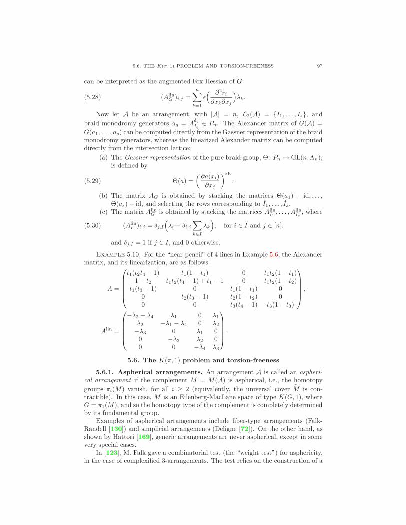
5.6. THE K(π, 1) PROBLEM AND TORSION-FREENESS 97
can be interpreted as the augmented Fox Hessian of G:
(5.28) (AlinG )i,j =
n∑
k=1
ǫ( ∂2ri∂xk∂xj
)λk.
Now let A be an arrangement, with |A| = n, L2(A) = I1, . . . , Is, and
braid monodromy generators αq = Aδq
Iq∈ Pn. The Alexander matrix of G(A) =
G(a1, . . . , as) can be computed directly from the Gassner representation of the braidmonodromy generators, whereas the linearized Alexander matrix can be computeddirectly from the intersection lattice:
(a) The Gassner representation of the pure braid group, Θ: Pn → GL(n,Λn),is defined by
(5.29) Θ(a) =
(∂a(xi)
∂xj
)ab
.
(b) The matrix AG is obtained by stacking the matrices Θ(a1) − id, . . . ,Θ(as)− id, and selecting the rows corresponding to I1, . . . , Is.
(c) The matrix AlinG is obtained by stacking the matrices Alin
I1, . . . , Alin
Is, where
(5.30) (AlinI )i,j = δj,I
(λi − δi,j
∑
k∈Iλk
), for i ∈ I and j ∈ [n].
and δj,I = 1 if j ∈ I, and 0 otherwise.
Example 5.10. For the “near-pencil” of 4 lines in Example 5.6, the Alexandermatrix, and its linearization, are as follows:
A =
t1(t2t4 − 1) t1(1− t1) 0 t1t2(1− t1)1− t2 t1t2(t4 − 1) + t1 − 1 0 t1t2(1− t2)
t1(t3 − 1) 0 t1(1 − t1) 00 t2(t3 − 1) t2(1 − t2) 00 0 t3(t4 − 1) t3(1− t3)
,
Alin =
−λ2 − λ4 λ1 0 λ1
λ2 −λ1 − λ4 0 λ2
−λ3 0 λ1 00 −λ3 λ2 00 0 −λ4 λ3
.
5.6. The K(π, 1) problem and torsion-freeness
5.6.1. Aspherical arrangements. An arrangement A is called an aspheri-cal arrangement if the complement M = M(A) is aspherical, i.e., the homotopy
groups πi(M) vanish, for all i ≥ 2 (equivalently, the universal cover M is con-tractible). In this case, M is an Eilenberg-MacLane space of type K(G, 1), whereG = π1(M), and so the homotopy type of the complement is completely determinedby its fundamental group.
Examples of aspherical arrangements include fiber-type arrangements (Falk-Randell [130]) and simplicial arrangements (Deligne [72]). On the other hand, asshown by Hattori [169], generic arrangements are never aspherical, except in somevery special cases.
In [123], M. Falk gave a combinatorial test (the “weight test”) for asphericity,in the case of complexified 3-arrangements. The test relies on the construction of a

98 5. FUNDAMENTAL GROUP
2-dimensional CW-complexK, which has the homotopy type ofM . This complex isa modified version of the Salvetti complex, and is built from information extractedfrom the real picture of the arrangement. The asphericity test (based on Gersten’sweight test, and work of Stallings on triangles of groups) involves assigning positivereal numbers around each vertex of the real diagram of the arrangement, so thatcertain conditions are satisfied.
Using Falk’s weight test, L. Paris showed that complexified, factored 3-arrange-ments are always aspherical.
5.6.2. Rational K(π, 1) arrangements.
5.6.3. Torsion-freeness. A group G is said to be torsion-free if it has noelement of finite order, besides the identity.
Question 5.11 (Orlik). Let G be an arrangement group. Is G torsion-free?
As is well-known, if a group G admits a finite-dimensional K(G, 1), then Gis torsion-free. Thus, if A is an aspherical arrangement, then its group, G(A), istorsion-free.
5.7. Residual properties
Let P be a class of groups. Following P. Hall, a group G is said to be residuallyP if, for every 1 6= g ∈ G, there is an epimorphism φ : G ։ H onto a group H ∈ Psuch that φ(g) 6= 1. In other words, every non-trivial element of G is detected in aquotient from P .
A related, yet stronger property, is as follows. A group G is fully residually Pif, for every finite subset S ⊂ G, there is an epimorphism φ : G ։ H onto a groupH ∈ P such that φ restricts to an injection on S. In this section, we discuss severalimportant cases of this notion, in the context of arrangement groups.
5.7.1. Residually finiteness and profinite completion. Let us writeH ≤fG for a finite-index subgroup of G, and similarly H ⊳f G for a normal, finite-indexsubgroup. Define the profinite completion of G as the inverse limit
(5.31) G := lim←−H⊳fG
G/H,
and let ιG : G → G the canonical homomorphism defined by ιG(g) = gH. Thefollowing result is well-known.
Proposition 5.12. For a group G, the following are equivalent:
(1) G is residually finite.(2)
⋂H:H≤fG
H = 1.(3)
⋂H:H⊳fG
H = 1.(4) ιG is injective.
The geometric motivation for this notion is as follows. Suppose X is a path-connected space, with fundamental group G = π1(X,x0). Then G is residuallyfinite if and only if any non-nullhomotopic loop at x0 can be realized as a non-trivial deck-transformation in a finite, regular cover of X .
Let G be a finitely generated group. Then G is residually finite if and only if itis Hopfian, i.e., every epimorphism G ։ G is an isomorphism. The automorphismgroup Aut(G) is again residually finite. And, finally, G has solvable word problem.

5.7. RESIDUAL PROPERTIES 99
Groups admitting faithful linear representations are residually finite. Well-known examples of residually finite groups are the finitely generated free groupsFn, the surface groups π1(Σg), and the Artin braid groups Bn. It is also knownthat all 3-manifold groups are residually finite. On the other had, infinite simplegroups are obviously not residually finite.
An old question attributed to J.-P. Serre asks whether fundamental groups ofcomplex algebraic varieties are residually finite. In [316], D. Toledo answered thisquestion, by producing examples of smooth projective varieties with non-residuallyfundamental groups. With these examples and counterexamples in mind, it isnatural to raise the following question.
Question 5.13. Let G be an arrangement group. Is G residually finite?
Question 5.14 (Suciu). Is the profinite completion of an arrangement groupcombinatorially determined? In other words, if A and A′ are two arrangements
with L(A) ∼= L(A′), is it true that G(A) ∼= G(A′)?
A related property of groups was introduced by J.-P. Serre in [292], and wasstudied in detail by Grunewald, Jaikin-Zapirain, and Zalesskii in [162]. A group
G is said to be good if the induced homomorphism ι∗G : H∗(G,M) → H∗(G,M)is an isomorphism, for every G-module M that is finite as a set. Goodness ispreserved under direct products, and is invariant under commensurability. Thefinitely generated free groups Fn, the braid groups Bn, and the pure braid groupsPn are all good. This naturally leads to the following question.
Question 5.15 (Suciu). Are arrangement groups good?
5.7.2. Residual nilpotency. IfG is a non-trivial, residually torsion-free nilpo-tent group, then G is indicable.
In [132], Falk and Randell showed that fundamental groups of fiber-type ar-rangements (in particular, the pure braid groups Pn) are residually (torsion-free)nilpotent. This naturally leads to the following question.
Question 5.16. Let G be an arrangement group.
(1) Is G residually nilpotent?(2) Is G residually torsion-free nilpotent?
By way of comparison, it is known that the braid groups of closed surfaces arenot always residually nilpotent. On the other hand, the pure braid groups of closedsurfaces are residually torsion-free nilpotent.
5.7.3. Residual freeness.
5.7.4. Virtual properties. A group G is said to be virtually P if G possessesa finite-index subgroup H ≤f G such that H belongs to the class P .


CHAPTER 6
Lie Algebras attached to arrangements
6.1. Lie algebras
6.1.1. Definition, examples, LCS and derived series. Multiplication ina ring A is an associative operation; if we remove this hypothesis and assume onlythat multiplication is bilinear, then the resulting object is a non-associative algebra.
Fix a field k of characteristic 0.
Definition 6.1. A Lie algebra g is a nonassociative algebra, such that thebilinear multiplication (denoted [·, ·], and called the (Lie) bracket) satisfies
• skew symmetry: [x, x] = 0• Jacobi identity: [x, [y, z]] + [z, [x, y]] + [y, [z, x]] = 0
For example, if V is a finite-dimensional k–vector space, then End(V ) becomesa Lie algebra if we define [M,N ] = MN − NM . More generally, if A is anyassociative algebra, we obtain a Lie algebra Lie(A) by defining a product in thisway.
Definition 6.2. For any k–algebra A, associative or non-associative, a deriva-tion (or k–derivation) is a homomorphism D of k–modules, D : A → A, satisfyingthe Leibnitz rule:
D(ab) = aD(b) + bD(a)
Denote the set of all derivations by Der(A); it is a k–module. In fact, Der(A) can begiven the structure of a Lie algebra, using the construction above: [D1, D2] (ab) =D1(D2(ab))−D2(D1(ab)).
6.1.2. Graded Lie algebras, free Lie algebra. Most of the Lie algebras wewill encounter, will have an additional structure—a grading, which is compatiblewith the Lie bracket.
Definition 6.3. A graded Lie algebra is a graded vector space g =⊕
k≥1 gk,
endowed with a Lie bracket [·, ·] satisfying
[gk, gm] ⊂ gk+m.
An important example is a free Lie algebra, which is defined as a Lie algebrasatisfying a universal property.
Definition 6.4. The free Lie algebra on a set B is the unique Lie algebra L(B)such that any Lie algebra g and k–module map from a free k–module on B to g
extends uniquely to a homomorphism of Lie algebras L(B)→ g.
This is a graded Lie algebra, with grading given by bracket length.
101

102 6. LIE ALGEBRAS ATTACHED TO ARRANGEMENTS
Example 6.5. If B is a finite set with 3 elementsx, y, z, then a basis for L(B)is:
bracket length i = 1 2 3 · · ·basis of L(B)i = x [x, y] [x, [x, y]]
y [x, z] [x, [x, z]]z [y, z] [y, [x, y]]
[y, [x, z]][y, [y, z]][z, [x, y]][z, [x, z]][z, [y, z]]
For n ∈ N, let µ(n) denote the Mobius function
µ(n) =
0 if n has repeat factors
1 if n = 1
(−1)k if n has k distinct prime factors.
Then the free Lie algebra on p generators has
1
m
∑
n|mµ(n)pm/n
monomials of degree m.
6.1.3. LCS and derived series.
Definition 6.6. An ideal of a Lie algebra g is a k–submodule h ⊆ g such that[g, h] ⊆ h. An ideal is itself a Lie algebra.
Clearly, [g, g] is an ideal, written g2, and if we define gn =[gn−1, g
], we obtain
a chain of ideals called the lower central series:
g ⊇ g2 ⊇ g3 ⊇ · · ·Definition 6.7. A Lie algebra is nilpotent if some gn = 0.
A second important series associated with g is the derived series:
g ⊇ g(2) = [g, g] ⊇ g(3) =[g(2), g(2)
]⊇ · · ·
Definition 6.8. A Lie algebra is solvable if some g(n) = 0.
put some examples here
6.1.4. Universal enveloping algebra and PBW. If g is a Lie algebra, thenthe universal enveloping algebra U(g) is an associative algebra which “envelops” g
gi→ U(g),
and possessing a universal property: for any associative algebra A and homomor-
phism gk→ A, there exists a unique map U(g)
j→ A such that ji = k. As Weibelnotes in [325], the construction of U(g) from g is similar in spirit to the construc-tion of the group ring from a group, and has similar consequences; for example thecategory of g–modules is isomorphic to the category of U(g)–modules.

6.2. QUADRATIC ALGEBRAS, KOSZUL ALGEBRAS, DUALITY 103
Definition 6.9. The universal enveloping algebra U(g) of a Lie algebra g isthe quotient of the tensor algebra T (g) by the relations
x⊗ y − y ⊗ x− [x, y]
Notice that if g is an abelian Lie algebra (all brackets are zero), then thisconstruction produces a symmetric algebra. In the last section, we saw that anarbitrary associative algebra A gives rise to a Lie algebra Lie(A). Let Lie denotethis functor; one can show ([325], Exercise 7.3.3) that the functors Lie and U areadjoint:
HomLie(g,Lie(A)) ∼= Homk-alg(U(g), A)
The most important theorem relating g and U(g) is the Poincare-Birkhoff-Witttheorem:
Theorem 6.10 (Poincare-Birkhoff-Witt). If ei are an ordered basis for g, theneI with I an increasing sequence are an ordered basis for U(g).
example here
6.2. Quadratic algebras, Koszul algebras, duality
In this section we give an overview of quadratic algebras and their duals, andalso discuss Koszul algebras and Koszul duality. A good quick reference is Exercise17.22 of [107], which we essentially reproduce in what follows. Let V be a finitedimensional k–vector space, and T = T (V ) the tensor algebra on V . A two sidedideal I ⊆ T (V ) is quadratic if it is generated by J ⊂ V ⊗ V ; in other words
I = T · J · T.A quotient T/I is a quadratic algebra if I is quadratic.
Definition 6.11. If J ⊂ V ⊗ V , define
J⊥ = a⊗ b ⊆ V ∗ ⊗ V ∗ | a(α) · b(β) = 0, ∀ α⊗ β ∈ JFor a quadratic algebra R = T (V )/J , the quadratic dual is R⊥ = T (V ∗)/J⊥.
Example 6.12. Let V have basis e1, . . . , en, and consider the ideal J =〈ei ⊗ ej − ej ⊗ ei〉. Then T (V )/J is the symmetric algebra Sym(V ). It is easy tosee that
J⊥ = 〈ei ⊗ ej + ej ⊗ ei, ei ⊗ ei〉(ei ⊗ ei obviously superfluous if char(k) 6= 2). So Sym(V )⊥ = Λ(V ∗).
Let V have basis e1, . . . , en. Given a quadratic algebra A = T (V )/J , wedefine the Priddy complex
P (A) : A // A⊗k A⊥1
// A⊗k A⊥2
// A⊗k A⊥3
// · · · ,with differential given by
α 7→ α ·n∑
i=1
ei ⊗ e∗i
By Exercises A3.28 and 17.22 in [107], it follows that A⊥ ∼= k⊗P (A); the cycles ink⊗P (A) are a subalgebra of k⊗P (A) which maps onto Ext∗A(k, k); multiplicationin Ext∗A(k, k) is the Yoneda product.

104 6. LIE ALGEBRAS ATTACHED TO ARRANGEMENTS
Definition 6.13. If M,N,P are R-modules, then the Yoneda product µ is amap:
ExtnR(N,P )⊗R ExtmR (M,N)µ // Extn+m
R (M,P ) .
Take a projective resolutions (Pi, di) for M and (Qi, δi) for N . An element ofExtmR (M,N) is θ ∈ Hom(Pn, N) such that θ dm+1 = 0; and an element ofExtnR(N,P ) is χ ∈ Hom(Qn, P ) such that χ δn+1 = 0. This gives a diagram:
Pm+1dm+1 // Pm
dm //
θ
Pm−1// · · ·
Qn+1δn+1 // Qn
δn //
χ
Qn−1// · · · // Q1
δ1 // Q0π // N
P
Since Pm is projective, there is a map Pmγm→ Q0 such that θ = π γm. Since
θ dm+1 = 0, we also have π γm dm+1 = 0, so that γm dm+1 maps Pm+1 to
the image of δ1. We obtain a map Pm+1γm+1→ Q1 such that γm+1 dm+2 has image
contained in the image of δ2. Iterating the process yields a commuting diagram:
Pm+n+1//
yyrrrrrrPm+n
//
xxrrrrrrr· · · // Pm+1
dm+1 //
γm+1xxxxx
xPm
dm //
θγmww
wwww
Pm−1// · · ·
Qn+1δn+1 // Qn
δn //
χ
Qn−1// · · · // Q1
// Q0π // N
P
The map Pm+nγm+n→ Qn satisfies im(γm+n dm+n+1) ⊆ im(δn+1). In particular,
χ γm+n dm+n+1 = 0, so that χ γm+n represents a class in Extn+mR (M,P ).
It follows from results of Lofwall (see [208]) that the map fromA⊥ to ExtA(k, k)
is injective, with image isomorphic to the “diagonal” Ext algebra⊕
i ExtiA(k, k)i.
Definition 6.14. A quadratic algebra is Koszul if A⊥ ∼= Ext∗A(k, k). This isequivalent to the condition that k has a minimal free resolution over A which islinear; linear means that the resolution has the form:
· · · // Ab3(−3) // Ab2(−2) // Ab1(−1) // A // k // 0 .
Since k has a linear resolution over A, b0 = 1 and we have that
1 = HS(k, t) = HS(A, t) ·∑
i≥0
(−1)ibiti.
Combining this with the isomorphism A⊥ ≃⊕i≥0 ExtiA(k, k)i yields:
Theorem 6.15. If A is a Koszul algebra, then HS(A, t) ·HS(A⊥,−t) = 1.
Example 6.16. Continuing with Example 6.12, if V is an n-dimensional vectorspace, then Koszul duality tells us that HS(Sym(V ), t) ·HS(Λ(V ),−t) = 1. As wehave seen that
HS(Sym(V ), t) =1
(1− t)n , and HS(Λ(V ), t) = (1 + t)n,
this is indeed the case.

6.4. THE ASSOCIATED GRADED LIE ALGEBRA OF AN ARRANGEMENT 105
6.3. Lie algebras attached to a group
To a finitely generated group G one can attach several graded Lie algebras,reflecting some of the structure of the group: the associated graded Lie algebra,the holonomy Lie algebra, and the Malcev Lie algebra. In this section, we discusseach one of these constructions, and how they relate to each other.
6.3.1. The associated graded Lie algebra.
Definition 6.17. The lower central series (LCS) of G is a chain of normalsubgroups,
G = γ1G ⊲ γ2G ⊲ γ3G ⊲ · · · ,defined inductively by γ1G = G, and for k ≥ 1,
γk+1G = [γkG,G].
Note that γk+1G is contained in the commutator subgroup of γkG. Thus, thequotient group grk(G) := γkG/γk+1G is abelian. Moreover, since G is finitelygenerated, grk(G) is also finitely generated. We will denote by
(6.1) φk(G) = rk grk(G)
the rank of the k-th LCS quotient of G.Now fix a field k of characteric 0.
Definition 6.18. The associated graded Lie algebra of G is the graded vectorspace
gr(G)⊗ k =⊕
k≥1
grk(G)⊗ k,
with Lie bracket induced from the commutator in G.
6.3.2. The holonomy Lie algebra. Again, for a field k (not of characteristic2 or 3) we may define the holonomy Lie algebra of a connected CW-complex X withfinite 1-skeleton to be the the free Lie algebra on H1(X, k), modulo the relationsimposed by the image of the dual of the cup product,
(6.2) H2(X, k)∪∗
// H1(X, k) ∧H1(X, k) .
Denote this Lie algebra by hX . For a finitely generated group G, define hG =hK(G,1). For a CW-complex X as above, with fundamental G = π1(X), it is readilychecked that hG = hX .
6.3.3. The Malcev Lie algebra and 1-formality.
6.4. The associated graded Lie algebra of an arrangement
Probably the most studied numerical invariants of an arrangement group G arethe ranks of its lower central series quotients, φk(G) = rk γkG/γk+1G. The impetuscame from the work of Kohno [195], who used rational homotopy theory to computeφk(Pℓ), the LCS ranks of the braid arrangement group. Falk and Randell [130],using more direct methods, established the celebrated LCS formula for the broaderclass of fiber-type arrangements, expressing φk(G(A)) in terms of the exponents ofthe arrangement A. Recent work by a number of authors has further clarified themeaning of this formula, and greatly expanded its range of applicability.

106 6. LIE ALGEBRAS ATTACHED TO ARRANGEMENTS
Let h = h(A) denote the rational holonomy Lie algebra of the complementM(A). Since M(A) is formal, k(A) is isomorphic to gr(π1(M(A))).
Since the cup product for arrangements is well understood, the image of (6.2)is easy to describe explicitly. Namely,
Proposition 6.19. For any arrangement A, the holonomy Lie algebra of M(A)is given by the presentation
h ∼= 〈xH | [xH′ ,∑
H∈XxH ]〉
with one generator for each H ∈ A, and with one relation for each X ∈ L2(A), andfor each H ′ ∈ X.
6.4.1. The Koszul property. While the fibre-type arrangements were knownto be K(π, 1) spaces, Falk observed that the converse did not hold by means of anexplicit calculation with the D4 arrangement: that is, not every K(π, 1) arrange-ment satisfied the LCS formula.
The paper of Shelton and Yuzvinsky [294] clarified the nature of the LCS for-mula by showing that it holds for those arrangements whose Orlik-Solomon algebrais Koszul. In particular, fibre-type arrangements have Koszul OS-algebras, and sothis recovers the LCS formula of Falk and Randell.
On the other hand, Papadima and Yuzvinsky [252] showed that the property ofan arrangement’s OS-algebra being Koszul (and hence satisfying the LCS formula)was equivalent to the complement M(A) being not a K(π, 1) but a rational K(π, 1).It became apparent that there were examples of arrangements whose complementswere rational K(π, 1) but not K(π, 1)’s, and vice-versa.
6.4.2. LCS resonance conjecture. In the late 1990s, tantalizing parallelsemerged to other, seemingly unrelated objects associated to the group G—namely,its resonance varieties. In [303], the following conjecture was formulated, expressing(under certain conditions) the ranks of the LCS quotients of G in terms of thedimensions of the components of the (first) resonance variety of G.
Write R1(G,C) = L1 ∪ · · · ∪ Lq, and set dimLi = di.
Conjecture 6.20 (Resonance LCS formula, [303]). Suppose φ4(G) = θ4(G).Then,
(6.3)
∞∏
k=2
(1 − tk)φk(G) =
q∏
i=1
1− dit(1− t)di
,
for k sufficiently large.
The conjecture has been verified for two important classes of arrangements:decomposable arrangements (essentially, those for which all components of R1
1(A)arise from sub-arrangements of rank two), and graphic arrangements (i.e., sub-arrangements of the braid arrangement); see [289, 249, 290, ?].
6.5. The Chen Lie algebra of an arrangement
Another direction was started by Cohen and Suciu [54, 57], with the study ofthe ranks of Chen groups of arrangements, θk(G) = φk(G/G
′′). The θ-invariantscan provide stronger information than the φ-invariants, distinguishing, in somecases, groups of fiber-type arrangements from the corresponding direct products offree groups.

6.6. THE HOMOTOPY LIE ALGEBRA OF AN ARRANGEMENT 107
6.5.1. The Chen ranks conjecture. Let A be a complex hyperplane ar-rangement, with complement X . As shown by Schenck and Suciu [289], the Chenranks of G = π1(X) are equal to the graded Betti numbers of the linear strand in aminimal, free resolution of the cohomology ring A = H∗(X, k), viewed as a moduleover the exterior algebra E on A:
(6.4) θk(G) = dimk TorEk−1(A, k)k, for k ≥ 2,
where k is a field of characteristic 0.
Conjecture 6.21 (Chen ranks conjecture, [303]). For k sufficiently large,
(6.5) θk(G) = (k − 1)∑
r≥1
hr
(r + k − 1
k
),
where hr is the number of r-dimensional components of the projective resonancevariety R1(A).
Work from [289] on the resolution of A over E and equality (6.4) yield a proofof the conjecture for graphic arrangements. In particular, this result recovers thecomputation of the Chen ranks of the pure braid groups from [54].
Example 6.22. If A = A(Kn) is the braid arrangement in Cn, then G isisomorphic to Pn, the pure braid group on n strings. Applying formula (7.25), wefind:
(6.6) θk(Pn) = (k − 1) ·(n+ 1
4
), for all k ≥ 3.
The Chen ranks of the pure braid groups were first computed in [54], using anarduous Grobner basis computation.
Using results on the geometry of R1(A) and a localization argument, Schenckand Suciu [290] establish the inequality
(6.7) θk(G) ≥ (k − 1)∑
r≥1
hr
(r + k − 1
k
), for k ≫ 0,
for arbitrary A. They show that there is a polynomial P (t) of degree equal to thedimension of R1(A), such that θk(G) = P (k), for all k ≫ 0.
The reverse inequality in (6.5) has an algebro-geometric interpretation in termsof the sheaf on Cn determined by the linearized Alexander invariant. The conjec-ture has been verified for two important classes of arrangements: decomposablearrangements (essentially, those for which all components of R1
1(A) arise from sub-arrangements of rank two), and graphic arrangements (i.e., sub-arrangements ofthe braid arrangement); see [249, 290].
6.6. The homotopy Lie algebra of an arrangement
This is a subtlety of rational homotopy theory that arises because π1(M(A)) isnot nilpotent in general, and this hypothesis is essential to comparing the homotopygroups of the rationalizationM(A) with the rationalized homotopy groups ofM(A).Consequently, the higher homotopy groups of an arrangement complement are notneatly determined by the cohomology ring A(A), even rationally. What is knownabout them is surveyed in [246, 247, 93].
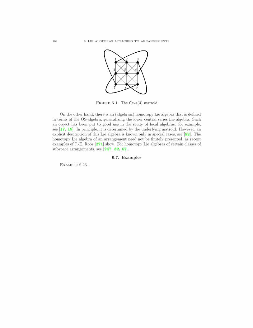
108 6. LIE ALGEBRAS ATTACHED TO ARRANGEMENTS
1 2 3
4 5 6
7 8 9
Figure 6.1. The Ceva(3) matroid
On the other hand, there is an (algebraic) homotopy Lie algebra that is definedin terms of the OS-algebra, generalizing the lower central series Lie algebra. Suchan object has been put to good use in the study of local algebras: for example,see [17, 19]. In principle, it is determined by the underlying matroid. However, anexplicit description of this Lie algebra is known only in special cases, see [82]. Thehomotopy Lie algebra of an arrangement need not be finitely presented, as recentexamples of J.-E. Roos [271] show. For homotopy Lie algebras of certain classes ofsubspace arrangements, see [247, 82, 67].
6.7. Examples
Example 6.23.

CHAPTER 7
Free Resolutions and the Orlik–Solomon algebra
7.1. Introduction
This chapter is devoted to free resolutions involving the Orlik-Solomon algebra;in particular the resolution of A and A∗ over the exterior algebra E, as well as theresolution of k over A. To simplify notation, throughout this chapter, we will write
bij = dimk TorEi (A, k)j
b∗ij = dimk TorEi (A∗, k)j
b′ij = dimk TorAi (k, k)j
and call these the graded Betti numbers. We begin in §7.2 by studying the numbersbij ; these numbers are computed from a minimal free E–resolution of A:
(7.1) P• : · · · //⊕
j Eb2j (−j) //
⊕j E
b1j (−j) // E // A // 0 ,
While determining the graded Betti numbers bij is an interesting problem in itsown right, further motivation is provided by a remarkable relation between thesenumbers and the fundamental group.
As we saw in Chapter 6, associated to the fundamental group of an arrange-ment complement there are certain graded Lie algebras. The ranks of the gradedcomponents of these algebras are two series of integers, the Chen ranks θk andthe LCS ranks φk. In §7.4 and §7.5 we describe the relations between the Chenand LCS ranks and homological invariants of the Orlik-Solomon algebra. If A isan essential, central arrangement in Cℓ, with complement M(A), and fundamentalgroup G = π1(M(A)), then:
(7.2) θk(G) = dimk TorEk−1(A, k)k, for k ≥ 2.
The LCS ranks φk(G) are also computed from certain Tor groups, but in aslightly more involved form:
(7.3)
∞∏
k=1
1
(1− tk)φk(G)=
∞∑
i=0
dimk TorAi (k, k)iti.
The point is that homological methods provide an alternative to the Lie-theoreticperspective on θk(G) and φk(G).
Open Problem 7.1. Give a formula for the numbers bij and b′ij . Formulasare known only for certain special classes of arrangements.
One important fact is that the regularity of A is bounded by the rank of A, sobij = 0 if j ≥ i+ rkA. In Chapter 5, we observed that if H is a generic C3, then
G = π1(M(A)) ≃ π1(M(A)|H)
109

110 7. FREE RESOLUTIONS AND THE OS–ALGEBRA
Thus, if the primary objective is to use the homological approach to study the Chenand LCS ranks of G, we can always restrict A to a generic C3, without changingθk(G) and φk(G). The regularity bound means that in this case only bi,i+1 andbi,i+2 may be non-zero.
In §7.3 we give a detailed treatment of the proof of [110] that A∗ ∼= annE(I)has a linear free resolution over E:
(7.4) · · · // Er2(−a− 2) // Er1(−a− 1) // Er0(−a) // A∗ // 0 .
The proof involves tools of combinatorial commutative algebra. As a consequence ofthis, Eisenbud-Popescu-Yuzvinsky also show that (as a complex of S–modules) theAomoto complex is exact; this follows from a powerful algebraic tool, the Bernstein-Gelfand-Gelfand (BGG) correspondence.
In §7.4 we describe BGG and how it can be used to prove (7.2), and sketchthe proof of a tight asymptotic lower bound for these ranks. For certain classes ofarrangements the bk−1,k can be described, and so Equation (7.2) yields the Chenranks.
In the final section, we describe the connections between the LCS ranks φk(G)and the numbers b′kk obtained from the minimal resolution of k over A. The genesisof (7.3) is Kohno’s result [195] for the φk(G) of the pure braid arrangement in Cn:
(7.5)
∞∏
k=1
(1− tk)φk = P (M(A),−t) =
n−1∏
i=1
(1 − it),
where P (M(A), t) =∑bit
i is the Poincare polynomial of the complement of M(A)in Cn. In [130], Falk and Randell give a generalization to fiber-type arrangements,i.e. those whose complement can be factored as a chain of linear fibrations withfiber Fi ≃ C \ p1, . . . , pik. As shown by Terao in [312], this is equivalent tosupersolvability of A. Supersolvability is equivalent to the existence of a quadraticGrobner basis for A, which implies that A is Koszul. In [294], Shelton and Yuzvin-sky interpret the LCS formula (7.3) in terms of Koszul duality.
If A is not Koszul, then there is no formula and no regularity bound for thenumbers b′ij ; compared to the numbers bij , they grow very quickly. In §7.5, werelate the two sets of numbers using the change of rings spectral sequence. Thefinal section describes differential graded algebras and Sullivan’s construction ofthe 1-minimal model of a DGA, which has a surprising connection to the spectralsequence.
7.2. Resolution of the Orlik-Solomon algebra over the exterior algebra
We start with an examination of the minimal free resolution of the Orlik-Solomon algebra over the exterior algebra. While no formula is known (in general)
for the numbers bij , the number b12 is obviously(b12
)− b2, so is easy to obtain.
Taking this as our cue, we begin by studying the numbers bi,i+1; these numbers aredetermined by the subcomplex
(7.6) F• : · · · // Eb34 (−4) // Eb23 (−3) // Eb12(−2)φ // E // A // 0 ,
of the minimal free resolution. The map φ is determined by any minimal setof generators for the quadratic component I2 of the Orlik-Solomon ideal I, andsubsequent differentials in the subcomplex are given by matrices of homogeneouslinear forms in E. We shall call F• the “2-linear strand” of the resolution.

7.2. RESOLUTION OF THE ORLIK-SOLOMON ALGEBRA OVER THE EXTERIOR ALGEBRA111
7.2.1. 2-linear Strand. As we saw in Chapter 1,
(7.7) dimAi = bi =∑
X∈Li(A)
(−1)iµ(X),
Since I is generated in degree ≥ 2, we have
(7.8) b12 =
(n
2
)− b2 =
∑
X∈L2(A)
(µ(X)
2
).
A is quadratic if b1j = 0 for j > 2. No explicit combinatorial formula for thenumbers b1j (j > 2) is known in general; but there is a regularity bound:
Lemma 7.2. Let A be an essential, central arrangement of rank ℓ. If j ≥ i+ ℓ,then
TorEi (A, k)j = 0.
Proof. To study the free E-resolution of A, we may pass to a decone of A.Let A′ = E′/I ′ be the OS-algebra of the decone. Then A′
j = 0, for j ≥ ℓ. The freeE′-resolution of k is linear, so after tensoring this resolution with A′, we obtain acomplex of modules with i-th term
⊕A′(−i), which vanishes in degrees i+ ℓ and
higher.
The importance of this is that the ith term in the free resolution P• of (7.1)has generators only in degrees between i+ 1 and i+ ℓ − 1. Since
∑
i
(−1)i∑
j
bijtj
· P (E, t) = P (A, t),
this means that if A consists of n hyperplanes in Cℓ, then
(7.9)
( ∞∑
i=0
ℓ−1∑
j=0
(−1)ibi,i+jti+j
)· (1 + t)n =
ℓ∑
i=0
biti
We now examine certain very simple syzygies in the 2–linear strand, which arisefrom those X ∈ L2(A) having µ(X) ≥ 2:
Example 7.3. Let A = H0, H1, H2 be an arrangement of 3 lines through theorigin of C2. The Orlik-Solomon ideal is generated by ∂e012 = (e1− e2)∧ (e0− e2).It is readily seen that the minimal free resolution of A over E is:
0← A←− E
“
∂e012
”
←−−−−−− F1
“
e1 − e2 e0 − e2
”
←−−−−−−−−−−−−−−− F2
0
@
e1 − e2 e0 − e2 00 e1 − e2 e0 − e2
1
A
←−−−−−−−−−−−−−−−−−−−−−−−− F3 ←−
· · · ←− Fi
0
B
B
B
@
e1 − e2 e0 − e2 0 · · · 0 00 e1 − e2 e0 − e2 · · · 0 0
0 0 0 · · · e1 − e2 e0 − e2
1
C
C
C
A
←−−−−−−−−−−−−−−−−−−−−−−−−−−−−−−−−−−−−−−−−− Fi+1 ←− · · ·
with Fi = Ei(−i− 1). Thus, bi,i+1 = i, for i ≥ 1, and bi,i+r = 0, for r > 1.
More generally, let A = H0, . . . , Hn be a central arrangement of n + 1 ≥ 3hyperplanes whose common intersection is of codimension two. The Orlik-Solomonideal is generated by all elements ∂eijk = (ej−ei)∧(ek−ei) with 0 ≤ i < j < k ≤ n.So A is quadratic, and a bit of linear algebra shows that (ej − e0) ∧ (ek − e0), for1 ≤ j < k ≤ n is a minimal set of generators. After a suitable linear change

112 7. FREE RESOLUTIONS AND THE OS–ALGEBRA
Figure 7.1. The arrangement X3 and its associated matroid
of variables, the ideal I becomes identified with the monomial ideal m2, wherem = (e1, . . . , en), and results of [7] show that only nonzero bij are given by:
(7.10) bi,i+1 = i
(n+ i− 1
i+ 1
), for all i ≥ 1,
Going back to an arbitrary arrangement, we observe that for each flat X ∈ L2(A)with µ(X) ≥ 2 there are linear syzygies of the type discussed in the examples above,which we will call local linear syzygies. In fact, these syzygies persist in the freeresolution of A over E, as the next lemma shows.
Lemma 7.4. Let A be an arrangement. Then:
(7.11) bi,i+1 ≥ i∑
X∈L2(A)
(µ(X) + i− 1
i+ 1
).
Moreover, if equality holds for i = 2, then it holds for all i ≥ 2.
Proof. Sets of local linear syzygies corresponding to different elements ofL2(A) are linearly independent. Indeed, they are supported only on generatorscoming from the same element of L2(A).
Lemma 7.4 suggests isolating the class of arrangements for which the 2–linearstrand of a minimal free resolution of A over E is wholly governed by the Mobiusfunction of L2(A).
Definition 7.5. An arrangement is called minimal linear strand (MLS) if
(7.12) b23 = 2∑
X∈L2(A)
(µ(X) + 1
3
).
For example, if A is an MLS arrangement of n hyperplanes in C3, then com-bining Lemma 7.4 and Equation 7.9 yields all the bij :
bi,i+1 = i∑
X∈L2(A)
(µ(X) + i− 1
i+ 1
)(7.13)
bi,i+2 = bi+1,i+2 +
(i+ 1
2
)(n+ i− 2
i+ 2
)−(n+ i− 2
i
) ∑
X∈L2(A)
(µ(X)
2
)(7.14)

7.2. RESOLUTION OF THE ORLIK-SOLOMON ALGEBRA OVER THE EXTERIOR ALGEBRA113
Example 7.6. Let A be the X3 arrangement, with defining polynomial Q =xyz(x − z)(y + z)(y + 2x), see Figure 5.3. We have X1, X2, X3 ⊆ L2(A) withµ(Xi) = 2, and so b12 = 3. Moreover, b13 = 1, and so condition (7.12) is satisfied.Equations 7.13 and 7.14 yield:
bi,i+1 = 3i
bi,i+2 =i(i+ 1)(i2 + 5i− 2)
8
A second class of examples where the numbers bi,i+1 can also be determinedexplicitly are graphic arrangements. Recall that Lemma 3.40 shows that b1j =|chordless (j + 1)-cycles of Γ|. As we saw in Chapter 3, the chromatic polynomialof Γ is equal to the characteristic polynomial of AΓ. Let κi denote the number ofcomplete subgraphs on i+ 1 vertices (the number of cliques in Γ). In [137], Farrellcomputes the first few coefficients for χ(A, t); combining those results with Lemma3.40 and a Hilbert series computation shows that:
b1 = κ1
b2 =(b12
)− b12
b3 =(b13
)− b1b12 − b13 + 2(κ2 + κ3)
It follows from this that there are b23 = 2(κ2 + κ3) linear first syzygies on thegenerators of I2. This is illustrated in the next example, and turns out to be thekey to understanding the 2–linear strand of any graphic arrangement.
•
•
e0
2222
2222
2222
2222
2
e1•
e2
•e3
e4DDD
DDDDDD
DD
e5zzz
zzzzzz
zz
Figure 7.2. The complete graph K4
Example 7.7. The complete graph K4 defines a central arrangement in C4
with defining equation ∏
1≤i<j≤4
(zi − zj).
Projecting along the subspace of C4 spanned by (1, 1, 1, 1) yields an essential, centralarrangementA in C3, with defining polynomial Q = xyz(x−y)(x−z)(y−z). Fromthe matroid in Figure 7.2, it is easy to see that
〈∂e145, ∂e235, ∂e034, ∂e012, ∂eijkl〉 = I,
where ijkl runs over all four-tuples; the elements ∂eijkl are consequences of thequadrics, so are redundant. The free resolution of A as a module over E begins:
0 Aoo Eoo E4(−2)∂1oo E10(−3)
∂2oo · · ·oo ,
where ∂1 =(∂e145 ∂e235 ∂e034 ∂e012
), and ∂2 =

114 7. FREE RESOLUTIONS AND THE OS–ALGEBRA
0 1
2
4
35
5
4
1
3
2
0
Figure 7.3. The braid arrangement and its matroid
0
B
B
B
B
@
e1 − e4 e1 − e5 0 0 0 0 0 0 e3 − e0 e2 − e0
0 0 e2 − e3 e2 − e5 0 0 0 0 e0 − e1 e0 − e4
0 0 0 0 e0 − e3 e0 − e4 0 0 e1 − e5 e2 − e5
0 0 0 0 0 0 e0 − e1 e0 − e2 e3 − e5 e4 − e5
1
C
C
C
C
A
.
To see this, write the generators of I2 as fi = αi∧βi (i = 1, . . . , 4); for example,f1 = ∂e145 = (e1 − e4) ∧ (e1 − e5). Each fi generates two local linear syzygies, αiand βi, which appear in columns 2i− 1 and 2i of the matrix ∂2. Let
η1 = e0 − e1 − e3 + e5 and η2 = e0 − e2 − e4 + e5.
A check shows that η1 ∧ η2 = f1 − f2 + f3 + f4 ∈ I2, which gives rise to a pairof linear syzygies, refecting the fact that ηi ∧ (η1 ∧ η2) = 0 in E3. Reducing thesetwo syzygies by the eight local linear syzygies yields the last two columns of ∂2.It is easy to see that the columns of ∂2 are linearly independent. Since Γ is a K4,b23 = 2(κ2 + κ3) = 10. Hence, the columns of ∂2 form a complete set of linear firstsyzygies on I2; a computation shows that no minimal first syzygies are quadratic.
Each of these 5 pairs of linear syzygies generates i+1 (independent) linear i-thsyzygies. This is trivially true for the local syzygies; for example, the pair (αi, βi)yields αi∧αi = βi∧βi = αi∧βi+βi∧αi = 0 as linear second syzygies. This followsfor the remaining two linear syzygies by similar reasoning. There can be no otherlinear second syzygies, because any such syzygy would have to involve the last twocolumns, and in each entry of those columns, the variables which appear are distinctfrom the variables in the entry of the remaining columns. Hence, bi,i+1 = 5i, forall i ≥ 2. This result generalizes:
Lemma 7.8. [289] Let A = AΓ be a graphic arrangement. If i ≥ 2, then
bi,i+1 = i(κ2 + κ3).
Open Problem 7.9. Give a graph theoretic interpretation for the bij . Lemmas3.40 and 7.8 give such interpretations for b1j and bj,j+1. For example, b14 is thenumber of chordless pentagons, and b34 = 3(κ2 +κ3). So if we know χ(G), then wecan solve for b24. However, just as in the general case, there is no explicit formulafor the bij of a graphic arrangement.
7.2.2. Resonance and b23. In Chapter 4, we saw that the first resonancevariety R1(A) is defined via:
µ ∈ E1 | ∃λ ∈ E1, λ 6= c · µ with µ ∧ λ ∈ I2.R1(A) consists of decomposable two tensors in I2. Since
∂(eiejek) = (ei − ej) ∧ (ei − ek),

7.2. RESOLUTION OF THE ORLIK-SOLOMON ALGEBRA OVER THE EXTERIOR ALGEBRA115
the generators of I2 give components of R1(A), called the local components. Themost interesting components of R1(A) come from another source. Notice that inExample 7.7, it follows from the definition that the line in P(E1) spanned by thepoints η1 and η2 belongs to R1(A). As we saw in Chapter 4, components of R1(A)arise from neighborly partitions: a partition Π of the hyperplanes of A such thatfor any rank two flat Y ∈ L2(A) and any block π of Π,
(7.15) µ(Y ) ≤ |Y ∩ π| =⇒ Y ⊆ π,In Example 7.7, η1 and η2 correspond to the neighborly partition Π = (05|13|24).The upshot of this is that decomposable two tensors in I2 have two manifesta-tions: they correspond to components of R1(A), and they give rise to elements ofTorE2 (A, k)3 (possibly non-minimal).
Theorem 7.10. For an MLS arrangement, all components of R1(A) are local.
Proof. If there is non-local resonance, then there exist nonzero a, b ∈ E1 with0 6= a ∧ b ∈ I2. Say, I2 = (f1, . . . , fk), so a ∧ b =
∑cifi. Then 0 = a ∧ a ∧ b =
a ∧∑ cifi =∑
(cia ∧ fi). Hence,c1a...cka
·
(f1 . . . fk
)= 0,
and so we have a linear syzygy. We may assume c1 6= 0; since the syzygy involvesf1 = (er − es) ∧ (et − es) and, by assumption, all linear syzygies are local, theonly variables that can appear in a correspond to hyperplanes incident on the flatX ∈ L2(A) containing r, s, t. Now pick any fi corresponding to a flat Y ∈ L2(A)(so µ(Y ) ≥ 2) with Y 6= X . Since |X ∩ Y | ≤ 1, the element a must be equal tosome eu, which is impossible.
12
5
7 3
0
4
6
Figure 7.4. The deleted MacLane matroid
The converse to Theorem 7.10 is false. The deleted MacLane arrangement isa real arrangement of eight lines, with matroid as in Figure 7.4. The resonancevariety has 7 local components, corresponding to the triple points; a computationshows that b23 = 15, rather than 14. This jump can be explained by the partition(06|13|27|45), which is “almost” neighborly, though not neighborly.
Definition 7.11. A partition Π of A is almost neighborly if, for any rank twoflat Y ∈ L2(A) with µ(Y ) > 1 and any block π of Π,
(7.16) µ(Y ) ≤ |Y ∩ π| =⇒ Y ⊆ π.

116 7. FREE RESOLUTIONS AND THE OS–ALGEBRA
In characteristic zero, an almost neighborly partition cannot contribute toR1(A) (only neighborly partitions can contribute). However, computations in-dicate that a jump in the dimension of b23 is often related to the presence of almostneighborly partitions. It would be interesting to find an explicit formula.
7.3. The resolution of A∗
In this section, we give a detailed treatment of the proof that A∗ has a linearfree resolution over E. In contrast to the numbers b′ij studied in the previoussection, the entire story is known for the numbers b∗ij , and is quite beautiful. Theproof involves three main ingredients, and makes substantial use of combinatorialcommutative algebra, which we describe in depth in the next section. In [110],Eisenbud, Popescu, and Yuzvinsky show:
Theorem 7.12. If A is an essential, central arrangement of n hyperplanes inCℓ, then A∗ has a minimal linear free resolution over E,
· · · // Er2(n− 2− ℓ) // Er1(n− 1− ℓ) // Er0(n− ℓ) // A∗ // 0 ,
where the ri satisfy the formula∞∑
i=0
riti = (−1)ℓ
χ(A, t)(1− t)n .
7.3.1. Alexander duality and monomial ideals. Let ∆ be a simplicialcomplex on vertex set 1, . . . , n. Let S = k[x1, . . . , xn] be a polynomial ring, withvariables corresponding to the vertices of ∆, and define the Stanley-Reisner ideal:
(7.17) I∆ = 〈xi1 · · ·xik | [i1, . . . , ik] is not a face of ∆〉The Stanley-Reisner ring S∆ is S/I∆. It will be useful to have a primary decom-position of I∆; this is easily seen to be ([288], Chapter 5):
Theorem 7.13.
I∆ =⋂
[i1,...,ik] a minimal coface
〈xi1 , . . . , xik〉.
Recall that an S–module M is said to have a linear resolution if TorS0 (M, k) is
generated in a single degree, say j, and TorSi (M, k)m = 0 unless m = i + j. Themodule M is Cohen-Macaulay over S if depth(M) = dim(M), where depth(M) isthe maximal length of a sequence s1, . . . , sd ⊆ 〈x1, . . . , xn〉 such that si is not azero-divisor on M/〈s1, . . . si−1〉M . For M = S∆ there is a simple sufficient criterionon ∆ (shellability, discussed shortly) for the Cohen-Macaulay property. The otherkey result we’ll need is due to Eagon and Reiner [102], who showed that S∆ has alinear resolution exactly when the Alexander Dual ∆∗ is Cohen–Macaulay over k.
Definition 7.14. If ∆ is a simplicial complex on [n] = 1, . . . n, then theAlexander dual ∆∗ = [n]− σ | σ 6∈ ∆.
The Alexander dual consists of the complements of the nonfaces. ∆ and ∆∗
satisfy the the following version of Alexander duality (see [225], Theorem 5.6):
Hi−1(∆∗, k) ∼= Hn−2−i(∆, k)
The Stanley-Reisner ideal I∆∗ of the Alexander dual is obtained from the Stanley-Reisner ideal of I∆ by switching the roles of minimal generators and prime compo-nents. This is illustrated best by an example:

7.3. THE RESOLUTION OF A∗ 117
Example 7.15. Suppose ∆ has maximal faces [1, 2, 3], [1, 2, 4], [1, 3, 4], [2, 4, 5],[3, 4, 5]. The minimal nonfaces of ∆ are [2, 3, 5], [2, 3, 4], [1, 5]. Since [1, 5] isnot a face, [1, 4, 5], [1, 3, 5], [1, 2, 5] are also nonfaces of ∆, so ∆∗ has maximalfaces [1, 4], [1, 5], [2, 3], [2, 4], [3, 4]. This means that [1, 2], [1, 3], [2, 5], [3, 5],[4, 5] are non-faces of ∆∗ (by construction, these are also the cofaces of ∆), soI∆∗ = 〈x1x2, x1x3, x2x5, x3x5, x4x5〉. The resolution of S∆∗ is linear:
0 // S2(−4) // S6(−3) // S5(−2) // S // S∆// 0 .
By Theorem 7.13, the primary decomposition of I∆ = 〈x2x3x5, x3x4x5, x1x5〉 is
I∆ = 〈x1, x2〉 ∩ 〈x1, x3〉 ∩ 〈x2, x5〉 ∩ 〈x3, x5〉 ∩ 〈x4, x5〉,and “turning the primary components into monomials” yields I∆∗ .
A simplicial complex is pure if all the maximal faces are equidimensional; oneeasy fact is that if S∆ is Cohen-Macaulay, then ∆ is pure. A standard criterion fordetermining if a simplicial complex is Cohen-Macaulay is the concept of shellability.
Definition 7.16. Let ∆ be a pure simplicial complex. ∆ is shellable if thereexists an ordering of the maximal faces σ1, σ2, . . . , σn, such that
σi ∩⋃
j<i
σj
is a pure codimension one subcomplex of σi, for all i.
The following theorem follows from an easy induction ([225], Theorem 13.45):
Theorem 7.17. If ∆ is shellable, then S∆ is Cohen-Macaulay
Theorem 7.17 explains why the resolution in Example 7.15 is linear: the sim-plicial complex ∆ = [1, 2, 3], [1, 2, 4], [1, 3, 4], [2, 4, 5], [3, 4, 5] is the boundary of abipyramid, with a single triangle deleted. Simplicial polytopes are shellable, so thesymmetry of this example means it is irrelevant that one triangle was deleted, andhence ∆ is shellable, so Cohen-Macaulay.
7.3.2. Proof of the theorem. The proof of the theorem that A∗ has a linearresolution proceeds in three steps. The first step is to identify A∗ with annE(I).We obviously have
A∗ = H∗ ∼= Homk(H∗, k)
Now, H∗ has the structure of an E–module, via aφ(m) = φ(am). The functorHomk(•, k) is a dualizing functor (applying the functor twice yields the identity)on the category of E-modules. By [107], Theorem 21.1,
Homk(A, k) ∼= HomE(A,E)
Of course, since A is a principal E-module, any element of HomE(A,E) is given bymultiplication by an element a ∈ E, and necessarily a · I = 0. So HomE(A,E) ≃annE(I), and resolving A∗ means resolving the ideal J = annE(I).
The second step of the proof is surprising. In general, the graded Betti numbersof an ideal L are upper semicontinuous under a flat deformation of L, such as passingto the initial ideal in(L) (e.g. Thm 3.6 of [170]). Remarkably, for the ideal J above,the resolution of the initial ideal turns out to be linear. Of course, it remains toprove this, but the point is that since the graded Betti numbers can only jump,

118 7. FREE RESOLUTIONS AND THE OS–ALGEBRA
the fact that they vanish for in(J) means that they must also vanish for J . Inparticular, if in(J) has a linear resolution, then so does J .
This brings us to the last part of the proof. There is an exterior version E∆
of the Stanley-Reisner ring, and in [7], Aramova, Avramov and Herzog show thatE∆ has a linear resolution over E exactly when the Stanley-Reisner ring (over S)of ∆∗ is Cohen-Macaulay; this is an exterior analog of the Eagon-Reiner result. Asdiscussed in Chapter 1, there is a particularly nice basis for the OS-ideal I—thebroken circuit basis. With respect to degree-lex order, in(I) consists of the brokencircuits, and since they are exterior monomials, they correspond to the OS-ideal ofa simplicial complex ∆.
The claim now is that in(J) = annE in(I). This equivalent to the statementthat in(J) corresponds to the Alexander dual of in(I). To see this, consider thedescription of Alexander duality in Example 7.15; I∆ is a “monomialization” ofthe primary decomposition of I∆∗ : each monomial xi1 · · ·xik ∈ I∆ corresponds toa prime component 〈xi1 , . . . xik〉 in the primary decomposition of I∆∗ . So everymonomial in I∆ has at least one variable from every monomial in I∆∗ ; passing tothe exterior algebra, this means that I∆ annihilates I∆∗ ; it is easy to see that anymonomial in I∆ must have this form. Thus
in(I) = I∆ = annE I∆∗ = in(J)
It remains to show that ∆ is Cohen-Macaulay. A result of Provan and Billera[263] that the simplicial complex corresponding to the broken circuits of a matroidis shellable, so in(I) is Cohen-Macaulay, which proves that A∗ has a linear freeresolution. The computation of the ranks follows immediately from Equation 7.9,replacing A with A∗.
Finer invariants than the numbers b∗ij are the actual differentials in the complex.In [83], Denham and Yuzvinsky obtain results on the first two differentials, but thehigher differentials are not known.
7.4. The BGG correspondence
Let V be a finite-dimensional vector space over a field k. The Bernstein-Gelfand-Gelfand correspondence is an isomorphism between the category of linearfree complexes over the exterior algebra E =
∧(V ) and the category of graded free
modules over the symmetric algebra S = Sym(V ∗). We give an outline of the BGGcorrespondence, and refer to Chapter 7 of [108] for additional detail.
Let L denote the functor from the category of gradedE-modules to the categoryof linear free complexes over S, defined as follows: for a graded E-module P , L(P )is the complex
(7.18) · · · // Pi ⊗ Sdi // Pi+1 ⊗ S // · · ·
with differentials di : p⊗ 1→∑eip⊗ xi.
Similarly, let R denote the functor from the category of graded S-modules tothe category of linear free complexes over E: for a graded S-module M , R(M) isthe complex
(7.19) · · · // Homk(E,Mi) // Homk(E,Mi+1) // · · ·

7.4. THE BGG CORRESPONDENCE 119
Example 7.18. Let E = Λ(k3), with e0, e1, e2 an ordered basis of E1 and
e0∧e1, e0∧e2, e1∧e2 an ordered basis for E2. Then the differential S⊗E1d1→ S⊗E2
takes the form:
e0 7→ x1e1 ∧ e0 + x2e2 ∧ e0e1 7→ x0e0 ∧ e1 + x2e2 ∧ e1e2 7→ x0e0 ∧ e2 + x1e1 ∧ e2
As one might guess, the resulting complex is the Koszul complex:
0 −→ S ⊗ E0
2
6
6
6
4
x0
x1
x2
3
7
7
7
5
−−−−−→ S ⊗ E1
2
6
6
6
4
−x1 x0 0−x2 0 x0
0 −x2 x1
3
7
7
7
5
−−−−−−−−−−−−−−−→ S ⊗ E2
h
x2 −x1 x0
i
−−−−−−−−−−−−−→ S ⊗ E3
Example 7.19. Let M be the S–module Sym(k2)/〈x20, x0x1〉. E ⊗ M1
d1→E ⊗M2 takes the form:
x0 7→ x0x0 ⊗ e0 + x0x1 ⊗ e1x1 7→ x0x1 ⊗ e0 + x1x1 ⊗ e1
Here the complex is
0 −→ E ⊗ M0
2
4
e0
e1
3
5
−−−−−→ E ⊗ M1
h
0 e1
i
−−−−−−−→ E ⊗ M2
h
e1
i
−−−−→ E ⊗ M3
h
e1
i
−−−−→ · · ·
It is a theorem of [109] that the complex R(M) is exact at position i as soon asi > reg(M); this is visible above.
Having developed some intuition for BGG, we record a theorem of Eisenbud-Fløystad-Schreyer [109] which will play a key role.
Theorem 7.20. If M is a graded S–module and P is a finitely generated gradedE-module, then L(P ) is a free resolution of M iff R(M) is an injective resolutionof P .
7.4.1. The Eisenbud-Popescu-Yuzvinsky resolution.
Theorem 7.21 ([110], Corollary 3.2). Define di via di(m) = (∑ei ⊗ xi) ∧m.
Then the following sequence of S–modules is exact:
(7.20) 0 // A0 ⊗ Sd0 // A1 ⊗ S
d1 // · · · dℓ−1 // Aℓ ⊗ S // F (A) // 0.
Proof. Apply the functor HomE(•, E) to the free resolution of H∗. As notedin the last section, since E is Gorenstein, injective resolutions over E are duals offree resolutions, and so we obtain an injective resolution of A. Let F (A) be theS-module which maps to this injective resolution—F (A) exists because we have anequivalence of categories. By Theorem 7.20, L(A) is a free resolution of F (A).
The key point here is that the complex obtained by applying BGG to A is infact exact, hence a free resolution of F (A). Notice that the differential di : p⊗ 1 7→∑ni=1 eip⊗ xi is precisely the differential in the Aomoto complex (A, a), where the
maps are given by multiplication by a generic linear form of the exterior algebra;the xi are simply the coefficients of this form.
Before proceeding, we point out an important detail. Throughout this book, Eis an exterior algebra generated in degree 1. In setting up the BGG correspondence,

120 7. FREE RESOLUTIONS AND THE OS–ALGEBRA
it is most natural to assume S = Sym(V ∗) is generated in degree one, and inthis case E =
∧(V ) is generated in degree −1. With these grading conventions,
in Theorem 4.3 of [109], Eisenbud, Fløystad and Schreyer show that if M is agraded S-module, with linear free resolution given by L(P ), then the dimension of
TorEi (P, k) can be computed from the dimensions of the graded pieces of certainlocal cohomology modules of M . As noted, in the context of arrangements, Eis generated in degree one, and it also turns out to be more natural to use Extmodules rather than local cohomology (which is possible by local duality). Withthese translations, we have:
Lemma 7.22. [290]
dimk TorEi (A, k)j = dimk Exti+ℓ−jS (F (A), S)j .
Recall that the regularity of an E-module M is the smallest integer n such thatTorEi (M, k)j = 0 for all i, j with j ≥ i + n + 1. Lemma 2.3 of [289] is that A is(ℓ−1)-regular; this also follows from Lemma 7.22 and the EPY resolution of F (A).
7.4.2. The module B as an Ext module. One of the motivating conjecturesof Chapter 6 is:
Conjecture 7.23 (Resonance formula for Chen ranks). Let G = G(A) be anarrangement group, and let hr be the number of components of the projective varietyR1(A) of dimension r. Then, for k ≫ 0:
(7.21) θk(G) = (k − 1)∑
r≥1
hr
(r + k − 1
k
).
In [57], Cohen and Suciu showed that the numbers θk(G) could be obtainedfrom the Hilbert series of the linearized Alexander invariant (over k). Recall fromChapter 6 that this is the S-module defined via the exact sequence
(A2 ⊕ E3)⊗ Sα2⊗id+δ3 // E2 ⊗ S // B // 0 ,
where αk : Ak → Ek is the adjoint of the canonical surjection γk : Ek ։ Ak (forsimplicity we write B instead of B ⊗ k).
Theorem 7.24. The linearized Alexander invariant is functorially determinedby the Orlik-Solomon algebra, as follows:
(7.22) B ∼= Extℓ−1S (F (A), S).

7.4. THE BGG CORRESPONDENCE 121
Proof. Consider the following commuting diagram, with exact rows and columns:(7.23)
0
0
0
0 // I2 ⊗ S
∂∗3 //
· · ·∂∗
ℓ−1// Iℓ ⊗ S //
F (I) //
0
0 // E0 ⊗ Sδ∗1 //
=
E1 ⊗ Sδ∗2 //
=
E2 ⊗ Sδ∗3 //
γ2
· · ·δ∗ℓ−1 // Eℓ ⊗ S //
γℓ
F (E) //
0
0 // A0 ⊗ Sd0 // A1 ⊗ S
d1 // A2 ⊗ S
d2 // · · · dℓ−1 // Aℓ ⊗ S
// F (A) //
0
0 0 0
The rows in the diagram are EPY resolutions. Notice that the middle rowis just a truncation of the Koszul complex over S. All columns but the last one(with solid arrows) are exact by definition of the Orlik-Solomon algebra A = E/I.The exactness of the two bottom rows, combined with the long exact sequence inhomology, shows that the rightmost column (marked with dotted arrows) is exact.This short exact sequence yields a long exact sequence of Ext modules:
· · · // ExtiS(F (E), S) // ExtiS(F (I), S) // Exti+1S (F (A), S) // · · ·
The Koszul complex is exact and self-dual, so ExtiS(F (E), S) = 0, for all i < ℓ,thus Exti+1
S (F (A), S) ∼= ExtiS(F (I), S), for i < ℓ − 1. Since all the vertical exactsequences (except the last one) consist of free S-modules, the dual sequences arealso exact, and so Ek/(imαk) ∼= (Ik ⊗ S)∗. Hence:
B = E2 ⊗ S/ im(α2 ⊗ id +δ3)
∼= (I2 ⊗ S)∗/ im(∂3)
∼= Extℓ−2S (F (I), S)
∼= Extℓ−1S (F (A), S).
If char k = 0 (which recall is our standing assumption), then we obtain:
Corollary 7.25. The Chen ranks of an arrangement group G equal the gradedBetti numbers of the linear strand of the cohomology ring A over the exterior algebraE:
(7.24) θk(G) = dimk TorEk−1(A, k)k, for all k ≥ 2.
Proof. We have:
θk(G) = dimk Bk by work of [57]
= dimk Extℓ−1S (F (A), S)k by Theorem 7.24
= dimk TorEk−1(A, k)k by Lemma 7.22.

122 7. FREE RESOLUTIONS AND THE OS–ALGEBRA
Combining Corollary 7.25 with Lemma 7.8 proves that Conjecture 7.23 holdsfor graphic arrangements.
Theorem 7.26. If G = π1(M(AΓ)) for a graph Γ, and κs = κs(Γ), then:
(7.25) θk(G) = (k − 1) (κ2 + κ3) , for all k ≥ 3.
7.4.3. Sketch of the lower bound on Chen ranks. As we saw in Chapter§5, the Chen ranks are determined by the dimension of the graded components ofthe linearized Alexander invariant B; in the last section we proved that for A ⊆ Cℓ
B ≃ Extℓ−1S (F (A), S) ≃ Extℓ−2
S (F (I), S).
We assume for the remainder of this section that ℓ = 3; there is no loss of generalityhere since the Chen ranks are completely determined by L2(A).
The strategy is to relate Ext1S(F (I), S) to Ext1S(F (I(Li)), S), for certain wellunderstood subideals I(Li) ⊆ I; the subideals I(Li) are determined by the reso-nance variety R1(A). From an algebraic viewpoint, there is no reason to distinguishbetween local and nonlocal components of R1(A)—both types of component corre-spond to a C-linear subspace of I2 consisting of decomposable two-tensors. Suppose
R1(A) =
m⋃
i=1
Li
As we saw in Chapter 4, the components Li are particularly nice:
Theorem 7.27 ([58], [206]). The defining ideal of R1(A) is the radical ofthe annihilator of the linearized Alexander invariant B. In characteristic zero, thecomponents of R1(A) are linear spaces which are disjoint in P(E1).
Now, each subspace Li corresponds to a subideal I(Li) of I2, hence there existsa short exact sequence of E–modules
0 // I(Li) // I2 // I2/I(Li) // 0 .
Applying BGG and using the results of §7.3 yields a commutative diagram of S-modules
(7.26) 0
0
0 // I(Li)2 ⊗ S //
I(Li)3 ⊗ S //
F (I(Li)) // 0
0 // I2 ⊗ S //
I3 ⊗ S //
F (I) // 0
0 // K1// I2/I(Li)2 ⊗ S //
I3/I(Li)3 ⊗ S //
F (I/I(Li)) // 0
0 0

7.5. RESOLUTION OF k OVER THE ORLIK-SOLOMON ALGEBRA 123
The modules in the middle two columns are free, so the first two rows are in factfree resolutions of F (I(Li)) and F (I). Dualizing gives a commutative diagram
0 0
0 Ext1S(F (I(Li)), S)oo (I(Li)2 ⊗ S)∗oo
OO
(I(Li)3 ⊗ S)∗oo
OO
F (I(Li))∗oo 0oo
0 Ext1S(F (I), S)oo (I2 ⊗ S)∗oo
OO
(I3 ⊗ S)∗oo
OO
F (I)∗oo 0oo
0 K2oo (I/I(Li)2 ⊗ S)
∗oo
OO
(I3/I(Li)3 ⊗ S)∗oo
OO
F (I/I(Li))∗oo 0oo
0
OO
0
OO
The snake lemma yields an exact sequence
0 // F (I/I(Li))∗ // F (I)∗ // F (I(Li))
∗
K2
// Ext1S(F (I), S) // Ext1S(F (I(Li)), S) // 0.
In particular, the map from Ext1S(F (I), S) to Ext1S(F (I(Li)), S) is surjective. Tak-ing the direct sum of these maps over all Li ∈ R1(A) gives an exact sequence
(7.27) Ext1S(F (I), S) //⊕
Li∈R1(A)
Ext1S(F (I(Li)), S) // C // 0,
where C is the cokernel. If we localize this sequence at the prime ideal Pi ⊆ Swhich is the ideal of Li, it yields
(7.28) Ext1S(F (I), S)Pi// Ext1S(F (I(Li)), S)Pi
// 0,
since the Li are projectively disjoint. In particular, C can be supported only at theirrelevant maximal ideal, from which it follows that the module C is of finite length,so vanishes in high degree. Hence, the Hilbert polynomial of B ≃ Ext1S(F (I), S)is bounded below by the sum of the Hilbert polynomials of Ext1S(F (I(Li)), S),yielding
Theorem 7.28. For k sufficiently large,
θk(G) ≥ (k − 1)∑
Li∈R1(A)
(dimLi + k − 1
k
).
Using similar techniques, it can be shown [290] that there is a rational poly-nomial P (k) such that P (k) = θk for k ≫ 0, with the degree of P (k) equal to thedimension of the projective variety R1(A).
Open Problem 7.29. Prove the other direction of the inequality.
7.5. Resolution of k over the Orlik-Solomon algebra
In this section, we study the numbers b′ii = dimk ExtiA(k, k)i = dimk TorAi (k, k)iobtained from the linear strand of the free resolution of the residue field k, viewed

124 7. FREE RESOLUTIONS AND THE OS–ALGEBRA
as a module over A. These numbers contain all the information about the LCSranks of an arrangement group, via the following formula of Peeva [256]:
(7.29)
∞∏
k=1
(1− tk)−φk =
∞∑
i=0
b′iiti.
The proof runs as follows. In [194], Kohno showed that the left hand quantity isequal to the Hilbert series of the universal enveloping algebra, U = U(g), of theholonomy Lie algebra g of the complement M(A). This follows from the Poincare-Birkhoff-Witt theorem, together with the isomorphism gr(G) ⊗ k ∼= g, which is aconsequence of the formality of M(A), in the sense of Sullivan. In [294], Shelton
and Yuzvinsky proved that U = A!, the Koszul dual of the quadratic closure of the
Orlik-Solomon algebra. Finally, results of Priddy [260] and Lofwall [208] relate theKoszul dual of a quadratic algebra to the linear strand in the Yoneda Ext-algebra:
(7.30) A! ∼=
⊕
i
ExtiA(k, k)i.
Since obviously ExtiA(k, k)i = ExtiA(k, k)i, formula (7.29) follows at once.
If A is a Koszul algebra, then A = A, and the Koszul duality formula, P (A!, t) ·P (A,−t) = 1, yields the LCS formula (7.3). This computation applies to supersolv-able arrangements, which do have Koszul OS-algebras, cf. [294]. The more generalformula (7.29) was first exploited by Peeva in [256] to obtain bounds on the LCSranks φk by deforming A to E/ ∈ (I).
The numbers b′ij are related to the numbers bij by the change of rings spectralsequence associated to the composition E → A ։ k:
(7.31) TorAi(TorEj (A, k), k
)=⇒ TorEi+j(k, k).
The utility of this is that the ranks of the modules appearing in a free resolution ofA over E are typically much smaller than the ranks of the free modules appearingin the resolution of k over A. In terms of the relation of the LCS ranks to theresolution of A over E, it is immediate that φ1 = b1 and φ2 = b12. In [118], Falkused the 1–minimal model to obtain a formula for φ3, which can be interpreted asφ3 = b23. Using the spectral sequence yields:
(7.32) φ4 =
(b122
)+ b34 − δ4,
where δ4 denotes the number of minimal quadratic syzygies on the degree 2 gener-ators of I which are Koszul syzygies. This has a nice interpretation in terms of the1−minimal model of A.
7.5.1. The change of rings spectral sequence. We start with a quickreview of the change of rings spectral sequence. Consider the composition of ringmaps:
E → A ։ k.
By taking a free resolution Q• for k over E and a free resolution P• for k over Aand tensoring with k, we obtain a first quadrant double complex, which yields aspectral sequence
(7.33) 2Eij ∼= TorAi(TorEj (A, k), k
)=⇒ TorEi+j(k, k).

7.5. RESOLUTION OF k OVER THE ORLIK-SOLOMON ALGEBRA 125
Since 1horE
i,j = 0 unless i = 0,
(7.34) 2horE
i,j = ∞horE
i,j .
In our situation (with E → A the canonical projection of the exterior algebraonto the OS-algebra, and A ։ k the projection onto the residue field), we have
(7.35) 2horE
0,j = TorEj (k, k),
and we can compute this term from the Koszul complex. In particular, TorEj (k, k)is nonzero only in degree j, and thus
(7.36) dimk TorEj (k, k)j =
(b1 + j − 1
j
).
We display the 2vertE
i,j terms:
TorE2 (A, k) TorA
1 (TorE2 (A, k),k) TorA
2 (TorE2 (A,k), k) TorA
3 (TorE2 (A, k),k)
TorE1 (A, k) TorA
1 (TorE1 (A, k),k) TorA
2 (TorE1 (A,k), k)
d2,12
jjUUUUUUUUUUUUUUUUUUUUUUUUUUU
TorA3 (TorE
1 (A, k),k)
k TorA1 (k,k) TorA
2 (k, k)
d2,02
jjUUUUUUUUUUUUUUUUUUUUUUUUUUUUTorA
3 (k,k)
d3,02
kkVVVVVVVVVVVVVVVVVVVVVVVVVVVVVV
d3,03
ii
From the diagram, we compute:
∞vertE
2,0 = ker d2,02
∞vertE
1,1 = cokerd3,02
∞vertE
0,2 = (coker d2,12 )/d3,0
3 (ker d3,02 )
Let tot be the total complex associated with the spectral sequence. We thenhave
gr(Hk(tot)) ∼=⊕
i+j=k
∞vertE
i,j ,
and thus
(7.37) gr(Hk(tot))r = 0, for r > k.
An easy exercise (see [107], Prop A3.25) shows that there is an exact sequencein low degree
TorE2 (k, k) // TorA2 (k, k) // TorE1 (A, k) // TorE1 (k, k) // TorA1 (k, k) // 0 .
Since TorEj (k, k) is concentrated in degree j, a check shows that this sequence is
also exact on the left, which implies that both ∞vertE
1,1 and ∞vertE
0,2 vanish. So:
im d3,02 = TorA1 (k,TorE1 (A, k)),
cokerd2,12 = d3,0
3 (ker d3,02 ).

126 7. FREE RESOLUTIONS AND THE OS–ALGEBRA
Tracing through the spectral sequence and using the equalities above, we obtainexact sequences
0y
∞vertE
3,0
y
0 −→ kerd3,02 −−−−→ TorA3 (k, k)
d3,02−−−−→ TorA1 (k,TorE1 (A, k)) −→ 0.
yd3,03
cokerd2,12y
0
Now recall that gr(H3(tot)) vanishes in degree greater than three, and so, inparticular,
(∞vertE
3,0)4
= 0. This proves:
Theorem 7.30. The following sequence is exact:
(7.38) 0 // (cokerd2,12 )4 // TorA3 (k, k)4 // TorA1 (k,TorE1 (A, k))4 // 0 .
Since the dimension of TorA1 (k,TorE1 (A, k))4 is b1b13, this contribution to b′34 =
dimk TorA3 (k, k)4 is easy to understand. We shall analyze the contribution from
dimk(coker d2,12 )4 next.
7.5.2. Quadratic syzygies and a Koszulness test. We have already seenthat if a3 > 0, then the algebra A is not Koszul. The sequence (7.38) gives anothernecessary condition for Koszulness. Indeed, if
(7.39) dimk TorE2 (A, k)4 > dimk d2,12 (TorA2 (k,TorE1 (A, k)))4,
then A is not a Koszul algebra. To apply this test, it is necessary to determine(im d2,1
2 )4. Recall that a Koszul syzygy on elements f1, . . . , fk ∈ Em is an element
of the submodule of ⊕ki=1Eǫi spanned by the(k2
)elements fjǫi + fiǫj . The space
of quadratic Koszul syzygies intersects the space TorE2 (A, k)3 ⊗ E1 (some Koszulsyzygies may be consequences of linear syzygies); we write K4 for the complementof this intersection. So K4 is the space of minimal quadratic syzygies which areKoszul.
Lemma 7.31. The image of d2,12 in degree 4 equals K4.
Proof. Take (minimal) free resolutions:
P• : 0←− k←− A←− Ab1(−1)←− A(b1+12 )(−2)⊕Aa2(−2)←− · · ·
Q• : 0←− k←− E ←− Eb1(−1)←− E(b1+12 )(−2)←− · · ·
and form the double complex

7.5. RESOLUTION OF k OVER THE ORLIK-SOLOMON ALGEBRA 127
P0 ⊗ (A⊗Q2) P1 ⊗ (A⊗Q2)
d
δoo P2 ⊗ (A⊗Q2)
P0 ⊗ (A⊗Q1) P1 ⊗ (A⊗Q1) P2 ⊗ (A⊗Q1)
d
δoo
d2
ll
P0 ⊗ (A⊗Q0) P1 ⊗ (A⊗Q0) P2 ⊗ (A⊗Q0)
The d2 differential is just the differential from the snake lemma. Since all thegenerators of I2 may be written as products of linear forms, the result follows froma diagram chase.
In view of this, we rephrase the non-Koszul criterion (7.39): If the minimalresolution of A over E has minimal quadratic non-Koszul syzygies, then A is not aKoszul algebra. The dimension of K4 can be bounded in terms of L(A).
Lemma 7.32.
(7.40) dimkK4 ≤∑
(X,Y )∈(L2(A)2 )
(µ(X)
2
)(µ(Y )
2
).
where(S2
)denotes the set of unordered pairs of distinct elements of a set S. More-
over, if A is MLS, then equality holds in (7.40).
Proof. Quadratic Koszul syzygies between elements of I2 which come from thesame dependent set are consequences of linear syzygies (because the free resolutionfor pencils is linear). Any two distinct elements of L2, say X and Y , give rise to(µ(X)
2
)(µ(Y )
2
)quadratic Koszul syzygies, and the bound follows. In the MLS case,
all linear syzygies come from pencils, hence any of the above Koszul syzygies is nota consequence of the linear syzygies.
7.5.3. Computing b′ii. The basic idea is to divide the problem up, using theexact sequence
(7.41) 0 // ker di,02// TorAi (k, k)i // im di,02
// 0 .
We start by analyzing the kernel of di,02 , illustrating the method in the i = 4case. Using the fact that the differentials in the spectral sequence are graded, we

128 7. FREE RESOLUTIONS AND THE OS–ALGEBRA
obtain the following diagram:
TorE3 (A, k)4
• TorA1 (k, TorE
2 (A, k))4
• • TorA2 (k,TorE
1 (A, k))4
• • • TorA4 (k,k)4
d2
ffMMMMMMMMMMMMMMM
d3
ggOOOOOOOOOOOOOOOOOOOOOOOOOOOOOOOOOOOOOO
d4
hhPPPPPPPPPPPPPPPPPPPPPPPPPPPPPPPPPPPPPPPPPPPPPPPPPPPPPPPP
Now recall from (7.37) that gr(H4(tot))r = 0 if r > 4. An analysis of the terms in⊕i+j=4
∞vertE
i,j shows that ∞vertE
4,0 = ker d4 is the only nonzero term and
dimk∞vertE
4,0 = dimk TorE4 (k, k)4 =
(b1 + 3
4
).
From the diagram
0y
0 −→ kerd4 −−−−→ ker d3 −−−−→ TorE3 (A, k)4 −→ 0y
ker d2y
TorA1 (k,TorE2 (A, k))4y
0
we find that
dimk kerd4,02 =
(b1+3
4
)+ b34 + b1b23.
In the general case, we obtain the following.
Lemma 7.33. dimk kerdi,02 =
(b1 + i− 1
i
)+
i−3∑
j=0
b′jjbi−j−1,i−j .

7.5. RESOLUTION OF k OVER THE ORLIK-SOLOMON ALGEBRA 129
Next, we analyze the image of di,02 . From the diagram
0y
(3vertE
i−2,1)iy
0 −→(im di,02
)i
d2−−−−→ TorAi−2(k,TorE1 (A, k))i −−−−→(cokerdi,02
)i−→ 0
y(im di−2,1
2
)iy
0
we obtain the following.
Theorem 7.34. Let δi = dimk(cokerdi,02
)i. Then:
bii + δi =
(b1 + i− 1
i
)+
i−2∑
j=0
b′jjbi−j−1,i−j .
Notice that dimk TorAi−2(k,TorE1 (A, k))i = b′i−2,i−2b12 has been incorporated in
the summation. The point is that the numbers b′ii can be computed inductivelyfrom the numbers bj,j+1 and δj ; ignoring δj yields an upper bound on the b′ii. Inthe case i = 4, (
3vertE
2,1)4
=(∞
vertE2,1)4.
By Equation 7.37
(∞vertEi,j)k
= 0 if k 6= i+ j,
so this term must vanish. So δ4 = dimk im(d2,12
)4; by Lemma 7.31 this equals
dimkK4, yielding:
Corollary 7.35.
(7.42) b′44 =
(b1 + 3
4
)+
((b1 + 1
2
)+ b12
)b12 + b34 + b1b23 − δ4
Combining formula (7.29) and the values for φk, k ≤ 3 yields a formula for φ4:
(7.43) φ4 =b1(b
31 − 6b21 − b1 − 2)
8− b1(3b1 + 1)
2b12−
(b12 + 1
2
)−b1(b13+b3)+b
′44.
By using (7.42) and (7.43), we can simplify this to:
Theorem 7.36. The rank of the fourth LCS quotient of an arrangement groupG is given by:
(7.44) φ4(G) =
(b122
)+ b34 − δ4.

130 7. FREE RESOLUTIONS AND THE OS–ALGEBRA
7.6. Connection to DGAs and the 1-minimal model
One of the basic theorems of algebraic topology is that the first integral homol-ogy group of a space is the abelianization of the fundamental group of the space. Itis natural to ask if one can extract more information about the fundamental group;work of Sullivan [305] shows that we can recover the lower central series ranks ofπ1(X) from the rational cohomology ring of X . This is explained in the topologyappendix; in what follows we describe the purely algebraic constructions that makesuch an operation possible.
Definition 7.37. A graded A0–algebra A = ⊕i≥0Ai is graded–commutative iffor x ∈ Ai, y ∈ Aj ,
xy = (−1)ijyx.
Definition 7.38. A differential graded algebra (DGA) (A, d) is a graded–commutative A0–algebra
A =⊕
i≥0
Ai
possessing a differential d : Ai → Ai+1 with d2 = 0. The differential is also requiredto act as a graded–commutative derivation
d(ab) = d(a) · b+ (−1)deg(a)a · d(b).Unless stated otherwise, A is assumed to be associative with unit.
In all the applications in this book, A0 will be one of Q,R,C. Standardexamples of DGA’s are the de Rham complex of C∞ forms on a manifold M , andthe de Rham complex of Q–polynomial forms on a simplicial complex ∆. If A isa DGA, then we write H∗(A) to denote the cohomology of A; it is itself a DGA,with differential zero. Let I = ⊕i>0Ai be the augmentation ideal of A; d is said tobe decomposable if d(A) ⊆ I2.
7.6.1. Minimal model of a DGA. The object that relates the cohomologyring H∗(X,Q) to the fundamental group of X is a ring known as the 1–minimalmodel of H∗(X,Q). To construct this ring, we need some preliminary definitions.Write Λn(V ) for the graded-commutative algebra generated by a finite dimensionalvector space V , concentrated in degree n; Λn(V ) is a symmetric algebra if n is evenand an exterior algebra if n is odd.
Definition 7.39. If (A, dA) is a DGA and V is a finite dimensional A0–vectorspace, then an extension (or Hirsch extension) of a (A, dA) is a DGA
B ≃ A⊗A0 Λn(V ),
with dB|A = dA and dB(V ) ⊆ An+1.
It is easy to see that if A is free (as a graded-commutative algebra), then so isB, and dA is decomposable iff dB is decomposable.
Definition 7.40. Let M be a connected DGA. Then M is minimal if
M =⋃
i≥0
Ci,
with each Ci ⊆ Ci+1 a Hirsch extension, C0 = M0 = k, and each d decomposable.It follows that

7.6. CONNECTION TO DGAS AND THE 1-MINIMAL MODEL 131
• M is free (as a graded–commutative algebra)• d is decomposable
So a minimal algebra is a tensor product of exterior algebras (with generatorsin odd degrees) and symmetric algebras (with generators in even degrees).
Definition 7.41. Let A be a connected DGA. A k–minimal model for Ais a minimal DGA M, together with a DGA morphism M → A, inducing anisomorphism in homology in degrees less than k, and an inclusion in degree k + 1.
It is a theorem of Sullivan that the k–minimal model exists and is unique (up tothe notion of homotopy of DGA’s, see [73]). The existence is fairly straightforward;here is how Sullivan describes the construction (see [305]):
“Suppose that M(k) ρk→ A has been constructed so that ρk induces an isomor-phism on cohomology in degree ≤ k and an injection in degree k + 1. Then we’add’ cohomology toM(k) (if necessary) and map accordingly to ’make ρk onto’ indegree k + 1. Then we add variables to ’kill’ the kernel on cohomology in degreek + 2 and map accordingly. If there are terms in degree one then we may have toagain kill the kernel in degree k + 2, and again, and again. . . . The union of these
constructions is the desiredM(k+1) ρk→ A.”The connection of the 1–minimal model of a space to the fundamental group
is given by
Theorem 7.42 (Sullivan, [305]). Let X be a connected simplicial complex withfinitely generated rational cohomology ring H∗(X). Then the ranks of the LCSquotients of the fundamental group are given by the dimension of the vector spacesappearing in the construction of the 1–minimal model of H∗(X).
7.6.2. Construction of the 1-minimal model. We now describe in moredetail the construction of the one-minimal model M (1) of a DGA A. First, defineV1 = H1(A);
M(1)1 = Λ1(V1)
The differential on Λ1(V1) is zero; hence H1(M(1)1 ) → H1(A) is an isomorphism.
By definition, M(1)k+1 = M
(1)k ⊗ Λ1(Vk+1), where Vk+1 is ker(H2(M
(1)k ) → H2(A)).
Thus, V2 is the kernel of the map Λ2(V1) ≃ H1(A) ∧H1(A)→ H2(A), and
M(1)2 = Λ1(V1)⊗ Λ1(V2).
The differential on M(1)2 is zero on V1, and is defined on V2 by the inclusion V2
i→Λ2(V1); the space V2 is concentrated in degree one. To compute the differential on
M(1)2 , we use the property that the differential is a graded derivation, so
d(α ⊗ β) = d(α) ⊗ β − α⊗ d(β).

132 7. FREE RESOLUTIONS AND THE OS–ALGEBRA
In terms of graded pieces, the DGA M(1)2 is
k0 // V1
0 // Λ2(V1)0 // Λ3(V1)
⊕ ⊕ ⊕V2
i;;wwwwwwV1 ⊗ V2
d77oooooooo
Λ2(V1)⊗ V2
⊕ ⊕Λ2(V2)
d77ooooooo
V1 ⊗ Λ2(V2)
⊕Λ3(V2)
If α⊗ β ∈ V1 ⊗ V2, then since d vanishes on V1,
d(α ⊗ β) = d(α) ⊗ β − α⊗ d(β) = −α⊗ d(β) ∈ Λ3(V1).
Similarly, if α ⊗ β ∈ Λ2(V2), then d(α ⊗ β) = d(α) ⊗ β − d(β) ⊗ α ∈ Λ2(V1)⊗ V2.This vanishes exactly when α = β; in this case α ∧ β = 0. Thus, the kernel of the
map H2(M(1)2 )→ H2(A) is
V3 = ker(V1 ⊗ V2 → Λ3(V1)).
Define
M(1)3 = Λ1(V1)⊗ Λ1(V2)⊗ Λ1(V3)
and continue this process. The differentials become more involved as the construc-
tion proceeds; for example, in H2(M(1)3 ) there will be a term corresponding to the
kernel of the map [Λ2(V2)⊕ (V1 ⊗ V3)]→ [Λ2(V1)⊗ V2]. Setting
M (1) =⋃
i≥0
M(1)i
yields the 1–minimal model of the DGA A.
7.6.3. Connecting H2(M(1)3 ) to the resonance LCS conjecture. We re-
turn to the Orlik-Solomon algebra, and compute the next Hirsch extension. As
described above, in H2(M(1)3 ) there will be a term corresponding to the kernel of
the map
Λ2(V2)⊕ (V1 ⊗ V3)d−→ Λ2(V1)⊗ V2,
whereV1 = E1
V2 = I2V3 = TorE2 (A, k)3
So the kernel of d consists of quadratic Koszul syzygies which are non-minimal;
dimk ker(d) =
(b122
)− δ4
Another term which will contribute to H2(M(1)3 ) comes from the kernel of the map
V1 ⊗ V3 −→ Λ4(V1).
This map corresponds to multiplying linear first syzygies by linear forms, hence thekernel of the map corresponds to linear second syzygies, and has dimension b34. It

7.6. CONNECTION TO DGAS AND THE 1-MINIMAL MODEL 133
can be shown that there are no other contributions to H2(M(1)3 ), so that V4 has
dimension
b34 +
(b122
)− δ4,
as expected. So the change of ring spectral sequence gives a very nice interpretationof Hirsch extensions, at least in low degrees. It would be interesting to have a generalformula of this type.
We end with an observation relating the results of this chapter to the ResonanceLCS conjecture of Chapter 6. Theorem 7.36 shows that
φ4 = θ4 ↔(b122
)= δ4.
The hypothesis in the resonance LCS conjecture that φ4 = θ4 is therefor equivalentto requiring that the every one of the
(b122
)quadratic Koszul syzygies are actually
minimal. As we saw in Section 7.2, all the minimal first syzygies associated to acodimension two flat are linear. Thus, if there exists X ∈ L2(A) with µ(X) > 2,the inequality φ4 = θ4 fails to hold.


CHAPTER 8
Local systems on complements of arrangements
8.1. Three views of local systems
Definition 8.1. The following comprise a bundle of groups on a topologicalspace X :
(1) A collection Vx | x ∈ X of (additive) abelian groups Vx;(2) A collection of isomorphisms Γx,y : Vx → Vy in one-to-one correspondence
with homotopy classes of paths γx,y from x to y in X ;(3) If γx,y, γx,z, and γy,z are (homotopy classes of) paths in X , then the
isomorphism corresponding to the product path γx,y · γy,z is equal to thecomposition Γy,z Γx,y.
Example 8.2. If p : E → X is a fiber bundle, let Fx = p−1(x). Then thehomology groups Hk(Fx) of the fiber form a bundle of groups on X . Similarly,for k ≥ 2, the homotopy groups πk(Fx) of the fiber form a bundle of groups onX .
Note that condition 8.1.3 above implies that the isomorphism corresponding tothe identity path at x is the identity id : Vx → Vx, and that Γ−1
x,y = Γy,x : Vy → Vx.Condition 8.1.2 implies that if γx ∈ π1(X,x) is any loop based at x, then thecorresponding isomorphism Γx is an automorphism of Vx. Consequently, a bundleof groups on X determines a representation of the fundamental group of X .
Example 8.3. Let X = S1 be the circle, and let x0 and x1 be a pair ofantipodal points. Let γ0,1 and γ1,0 be counterclockwise paths from x0 to x1 andx1 to x0 respectively. Then the fundamental group π1(X,x0) is generated by the(homotopy class of the) loop γ = γ0,1 · γ1,0.
Given a bundle of groups Vx on X = S1, we have isomorphisms Γ0,1 : Vx0 →Vx1 and Γ1,0 : Vx1 → Vx0 . If V = Vx0 , the corresponding representation ρ :π1(X,x0)→ Aut(V ) is given by ρ(γ) = Γ, where Γ = Γ1,0 Γ0,1.
Conversely, given a representation ρ : π1(X,x0) → Aut(V ), there is a uniqueassociated bundle of groups Vx on X with Vx0 = V . This bundle of groups maybe constructed as follows. For each x ∈ X , fix a homotopy class of paths γx,x0 fromx to x0, and a corresponding isomorphism Γx,x0 : Vx → Vx0 = V . Then if γx,y is apath from x to y, define
(8.1) Γx,y = Γ−1y,x0 ρ(γ−1
x,x0· γx,y · γy,x0) Γx,x0 .
It is a straightforward exercise to check that the isomorphism Γx,y defined in (8.1)depends only on the homotopy class of the path γx,y, and that these isomorphismssatisfy the transitivity condition 8.1.3.
Assume that V is a vector space over a field. Then the representation ρ :π1(X,x0)→ Aut(V ) determines a vector bundle p : E → X over X as follows. The
135

136 8. LOCAL SYSTEMS ON COMPLEMENTS OF ARRANGEMENTS
fundamental group G = π1(X,x0) acts on the universal cover X of X by covering
transformations. Let E = X × V/G be the quotient space, where for (x, v) is
identified with (γ · x, ρ(γ)(v)) for (x, v) ∈ X × V and γ ∈ G. The map p : E → X
is the natural projection from E = X × V/G to X = X/G.The vector bundle p : E → X is flat in the sense that the transition functions
are locally constant. In other words, this vector bundle admits a flat connection.A connection on a vector bundle may be viewed as a means of comparing fibers byparallel translation, or as a means of differentiating sections. Let Ω0(E,X) denotethe sections of the vector bundle, and more generally, Ωk(E,X) the k-forms. Aconnection is a linear map ∇ : Ω0(E,X) → Ω1(E,X) which satisfies the Leibnitzrule ∇(fs) = df · s + f∇(s) for a function f and a section s. The connection ∇induces a map (also denoted by ∇) from Ωk(E,X)→ Ωk+1(E,X) for each k ≥ 1.The connection is said to be flat if the curvature ∇ ∇ : Ω0(E,X) → Ω2(E,X)vanishes. If ∇ is flat, then parallel transport about a loop in X depends only onthe homotopy class of the loop. Thus, a flat connection determines a (holonomy)representation of the fundamental group.
In what follows, we will discuss various aspects of the homology and coho-mology of the complement of an arrangement with coefficients in a local systemL. Depending on the perspective, these (co)homology groups can be investigatedin various ways. For instance, if the local system L is given by a representationρ : G→ Aut(V ) of the fundamental group G = π1(X), the local system homology
H∗(X ;L) is the homology of the complex C∗(X) ⊗G V , where X is the universalcover of X . If L is given by a flat connection ∇ on a vector bundle p : E → X , thelocal system cohomology is the cohomology of the complex (Ω∗(E,X),∇). If L isgiven by a bundle of groups on X , then, for example, the singular chain complexC∗(X,L) is constructed as follows. Let Ck(X ;L) be the set of all functions c suchthat c(u) ∈ Vu(e0) for all singular k-simplices u : ∆k → X , and c(u) = 0 for all butfinitely many u. The boundary map ∂ : Ck(X ;L)→ Ck−1(X ;L) is defined by
∂(ξu) = Γu(e0),u(e1)(ξ)∂0(u) +
k∑
i=1
(−1)iξ∂i(u)
on elementary chains ξu, where u is a k-simplex and ξ ∈ Vu(e0), and extendinglinearly. Analogous constructions may be made for other homology theories.
Example 8.4. Recall the antipodal points x0 and x1, and the paths γ0,1 andγ1,0 between them on the circleX = S1 from Example 8.3. Define singular simplicesu0j : ∆0 → S1 and u1
j : ∆1 → S1 by u0j = xj , u
10(t) = γ0,1(t), and u1
1(t) = γ1,0(t).
Given a bundle of groups Vx on S1, recall that we denote the isomorphismscorresponding to the paths γp,q by Γp,q. For k = 0, 1, the singular chain groups are
Ck(S1;L) = v0 · uk0 + v1 · uk1 | vj ∈ Vuk
j (e0),
and the boundary map ∂ : C1(S1;L)→ C0(S
1;L) is given by
∂(v0 · u10 + v1 · u1
1) = Γu10(e0),u1
0(e1)(v0) · u00 − v0 · u0
0 + Γu11(e0),u1
1(e1)(v1) · u01 − v0 · u0
1
= Γ0,1(v0) · u01 − v0 · u0
0 + Γ1,0(v1) · u00 = v1 · u0
1
= (Γ1,0(v1)− v0) · u00 + (Γ0,1(v0)− v1) · u0
1.

8.2. GENERAL POSITION ARRANGEMENTS 137
Define automorphisms ψk : Ck(S1;L)→ Ck(S
1;L) by
ψ1(v0 · u10 + v1 · u1
1) = v0 · y10 + (Γ0,1(v0) + v1) · u1
1,
ψ0(w0 · u00 + w1 · u0
1) = (w0 + Γ1,0(w1)) · u00 − w1 · u0
1.
Then, a calculation reveals that
ψ0 ∂ ψ1(v0 · u10 + v1 · u1
1) = (Γ(x) − x) · u00 + y · u0
1,
where Γ = Γ1,0 Γ0,1 ∈ Aut(V ), and V = Vx0 . Thus, the local system homologyH∗(S1;L) is given by the homology of the complex
(8.2) VΓ−id−−−→ V.
This last complex may be realized as the complex resulting from the standard CWdecomposition of the circle, with a single zero cell and a single one cell.
Recall from Example 8.3 that the automorphism Γ of V determines the rep-resentation ρ : π1(S
1, x0) → Aut(V ) corresponding to the bundle of groups Vx.Additionally, the complex (8.2) is chain equivalent to C∗(R) ⊗Z V , where R is the
universal cover of S1 and Z = π1(S1) = 〈γ〉. The augmented chain complex C∗(R)
can be expressed as
ZZ γ−1−−−→ ZZ ǫ−→ Z,where ZZ is the group ring of Z = π1(S
1) and ǫ(γ) = 1. Note that this provides afree resolution of Z over ZZ.
More generally, let Y = (S1)n be the n-dimensional torus. The fundamentalgroup π1(Y ) is free abelian of rank n. Denote the generators by γ1, . . . , γn. Letρ : π1(Y ) → Aut(V ) be a representation, and L the corresponding local systemon Y . Note that the automorphisms Tj = ρ(γj), 1 ≤ j ≤ n, commute. A chaincomplex C∗(Y ;L) which computes the local system homology H∗(Y ;L) may bedescribed as follows.
Let R = ZZn be the group ring of Zn = π1(T ), and let C be a free R-module
with basis e1, . . . , en. Then the complex C∗(Y ;L) has terms Ck(Y ;L) =∧k
C⊗Vand boundary maps ∂k : Ck(Y ;L)→ Ck−1(Y ;L) given by
(8.3) ∂k(ei1ei2 · · · eik ⊗ v) =
k∑
j=1
(−1)j−1ei1 · · · eij · · · eik ⊗ (Tij − id)v
8.2. General position arrangements
One of the first studies of local systems on complements of arrangements wascarried out by Hattori [169]. Motivated by problems from the Aomoto-Gelfandtheory of hypergeometric integrals (see [244] for a modern exposition), he analyzedthe local system homology of complements of general position arrangements.
Let G = H1, . . . , Hn be an arrangement of n hyperplanes in general positionin Cℓ, with n ≥ ℓ. If I ⊂ [n] is a subset of cardinality k, then dim
⋂i∈I Hi = ℓ− k
if k ≤ ℓ and⋂i∈I Hi = ∅ if k > ℓ. In [169], Hattori showed that the complement
M = M(G) has the homotopy type of the ℓ-skeleton of the n-torus, and used thisresult to record the cellular chain complex C∗(M ;L) of X with coefficients in anarbitrary complex, rank one local system.
The fundamental group π1(M) is generated by meridian loops xj in M aboutthe hyperplanes Hj in Cℓ. If ℓ = 1 then π1(M) is free. If ℓ ≥ 2, then π1(M) isfree abelian. Let V ∼= Cm be a complex vector space, and let L be the complex

138 8. LOCAL SYSTEMS ON COMPLEMENTS OF ARRANGEMENTS
local system on X corresponding to the representation ρ : π1(M)→ Aut(V ). Notethat the automorphisms Tj = ρ(xj) commute in the case ℓ ≥ 2. The chain complexC∗(M ;L) may be realized as the truncation
V (nℓ) ∂ℓ−→ V ( n
ℓ−1) ∂ℓ−1−−−→ · · · ∂3−→ V (n2) ∂2−→ V (n
1) ∂1−→ V (n0),
with boundary maps ∂k given by (8.3), of the chain complex of the n-torus recordedin Example 8.4. Using this truncation, Hattori proves the following vanishing the-orem.
Theorem 8.5 (Hattori [169]). Let G = H1, . . . , Hn be a general positionarrangement of n hyperplanes in Cℓ with complement M , and L a complex localsystem on M with monodromy Tj ∈ Aut(V ) about Hj. If 1 is not an eigenvalueof Tj for some j, 1 ≤ j ≤ n, then Hq(M ;L) = 0 for q 6= ℓ, and dimC Hℓ(M ;L) =(n−1ℓ−1
)· dimC V .
Proof. Without loss, assume that 1 is not an eigenvalue of the monodromyautomorphism T1. Define Ψ : C∗(M ;L)→ C∗+1(M ;L) by
Ψ(eI ⊗ v) =
e1eI ⊗ (T1 − id)−1v if 1 /∈ I,0 otherwise.
Checking that ∂Ψ+Ψ∂ = 1, we conclude that Hq(M ;L) = 0 for q < ℓ. An Euler
characteristic argument then shows that dimCHℓ(M ;L) =(n−1ℓ−1
)· dimC V .
8.2.1. Homology of cyclic covers. Let pk : C∗ → C∗, pk(z) = zk, be thestandard cyclic k-fold covering. The Leray-Serre spectral sequence insures thatthe homology Hi(B;Hj(F )) abuts to Hi+j(E), where B = C∗ is the base of the
covering, E = C∗ is the total space, and F = p−1k (w), w ∈ B, is the fiber. Since the
fiber is discrete, we have Hj(F ) = 0 for j 6= 0, and H∗(B;L) ∼= H∗(E), where L is
the local system corresponding to the bundle of groups H0(p−1k (w)). Evidently,
the fundamental group of the base acts on the fiber by cyclically permuting thepoints, so acts on V = H0((p
−1k (w)) ∼= Zk analogously. In other words, the local
system L corresponds to the representation ρ : π1(C∗)→ Aut(V ) = GLk(Z) whichsends a generator to a cyclic permutation matrix of order k. We leave it to thereader to compute the homology of the total space, H∗(C∗) = H∗(C∗;L), by thesemeans.
More generally, let A be an arbitrary arrangement, with defining polynomialQ and complement M . Consider the cyclic k-fold covering Pk : Mk →M obtainedby pulling back the standard cyclic cover pk : C∗ → C∗:
Mk −−−−→ C∗
Pk
yypk
MQ−−−−→ C∗
The covering space Mk is given explicitly by
Mk = (x, z) ∈M × C∗ | Q(x) = zk.In the special case k = |A| + 1, the covering space Mk is homeomorphic to theMilnor fiber of the cone of A, see Chapter 11.
As above, the homology of the covering space Mk may be calculated using theLeray-Serre spectral sequence: H∗(Mk) = H∗(M ;L), where L is the local system

8.3. ASPHERICAL ARRANGEMENTS 139
corresponding to the bundle of groups H0(P−1k (x)). We subsequently focus on
complex coefficients. The local system L was identified in [53] and [48].
Proposition 8.6. Let T ∈ GLk(C) be the cyclic permutation matrix of orderk defined by T (~ei) = ~ei+1 for 1 ≤ i ≤ k − 1 and T (~ek) = ~e1, where ~ei is thestandard basis for Ck. Note that T is diagonalizable with eigenvalues ξqk, 1 ≤ q ≤ k,where ξk = exp(2π i /k).
(1) The local system L on M is induced by the representation ρ : π1(X) →GLk(C) given by ρ(γH) = T for each meridian γH .
(2) The local system L decomposes into a direct sum, L =⊕k
q=1 Lq of rankone local systems. For each q, the local system Lq is induced by the rep-resentation ρq : π1(M)→ C∗ defined by ρq(γH) = ξqk.
(3) The homology of the covering space Mk admits the direct sum decomposi-
tion H∗(Mk; C) =⊕k
q=1H∗(M ;Lq).
Note that the local system Lk is trivial. Consequently, the homology of M isa direct summand of that of Mk. For general position arrangements, Theorem 8.5may be used to calculate H∗(M ;Lq) for 1 ≤ q ≤ k − 1, yielding the homology ofMk.
Proposition 8.7. Let G ⊂ Cℓ be a general position arrangement of n > ℓhyperplanes. For k ≥ 1, the Betti numbers of the cyclic covering space Mk of thecomplement M are
bq(Mk) =
(n
q
)for q < ℓ, and bℓ(Mk) =
(n
ℓ
)+ (k − 1) ·
(n− 1
ℓ− 1
).
In the case k = n+1, this result yields the Betti numbers of the Milnor fiber ofa generic arrangement of n+1 hyperplanes in Cℓ+1, a result first obtained by othermeans by Orlik and Randell [239], and recovered by Massey [215] among others.
8.3. Aspherical arrangements
An arrangement A is said to be aspherical, or a K(G, 1)-arrangement, if thecomplement M is a K(G, 1)-space, where G = π1(M). For such arrangements,local systems may be studied from the point of view of (co)homology of groups, seeBrown [30] as a general reference.
Let A be a K(G, 1)-arrangement, and let L be the local system on the comple-ment of A corresponding to the representation ρ : G→ Aut(V ). The representationρ provides V with the structure of a ZG-module, and one has
H∗(M ;L) = H∗(G;V ) and H∗(M ;L) = H∗(G;V ),
the local system (co)homology of M is equal to the (co)homology of G with coeffi-cients in the module V . To justify this, observe that the augmented chain complex,
C∗(M)ǫ−→ Z, of the universal cover of M is a resolution of Z over ZG, and note
that, for instance, both H∗(M ;L) and H∗(G;V ) may be obtained by computing
the homology of the complex C∗(M)⊗G V .
Example 8.8. Let A be an arrangement of n distinct points in C. The comple-ment M has the homotopy type of a bouquet of n circles, and is a K(G, 1)-space,where G = π1(M) is a free group on n generators. Write G = Fn = 〈x1, . . . , xn〉.

140 8. LOCAL SYSTEMS ON COMPLEMENTS OF ARRANGEMENTS
The chain complex of the universal cover ofM provides a free resolution C∗(G)→ Zover ZG, given explicitly by
0→ (ZG)n∆−→ ZG ǫ−→ Z→ 0,
where ∆ =(x1 − 1 · · · xn − 1
)⊤and ǫ is the augmentation map, given by
ǫ(xi) = 1.Let ρ : G → Aut(V ) be a representation, with ρ(xi) = Ti, and L the corre-
sponding local system on M . Then H∗(M ;L) = H∗(G;V ) is the homology of thecomplex C∗(G) ⊗G V , given explicitly by
V nρ∗(∆)−−−−→ V,
where
ρ∗(∆) =
ρ(x1)− id
...ρ(xn)− id
=
T1 − id
...Tn − id
.
Note that A may be viewed as a “general position” arrangement, and that thecomplex C∗(G) ⊗G V may be realized as Hattori’s complex. Note also that theresolution C∗(G) is minimal in the sense that Ci(G) is a free ZG-module of rankbi(X) and the boundary map ∆ augments to 0.
The complement X = C \ n points of the arrangement in the previous ex-ample may be realized as the fiber of the classical Fadell-Neuwirth bundle pn,1 :Fn+1(C) → Fn(C), where Fn(C) is the configuration space of n ordered pointsin C, and pn,1(x1, . . . , xn, xn+1) = (x1, . . . , xn). More generally, the fiber of theFadell-Neuwirth bundle pn,ℓ : Fn+ℓ(C) → Fn(C) may be realized as the com-plement X(An,ℓ) of a discriminantal arrangement in the sense of Schechtman-Varchenko [285].
The fundamental group of the configuration space Fn(C) is the Artin purebraid group on n strands. Since the Fadell-Neuwirth bundle admits a section, thehomotopy exact sequence of the bundle can be used to show that the pure braidgroup Pn is an iterated semidirect product of free groups,
Pn = Fn−1 ⋊αn−1 Fn−2 ⋊ · · ·⋊ F2 ⋊α2 F1.
The monodromy homomorphism αk : Pk → Aut(Fk) is given by the restrictionof the Artin representation to the pure braid group. Let Ai,j be the pure braidobtained by performing a full twist on strands i and j (behind the others strands).Then, if Fk = 〈x1, . . . , xk〉, we have
(8.4) Ai,j(xq) =
xq if q < i or q > j,
xixjx−1i if q = j,
xixjxix−1j x−1
i if q = i,
[xi, xj ]xq[xi, xj ]−1 if i < q < j
Similarly, the fundamental group of the complement of the discriminantal arrange-ment may be realized as
π1(X(An,ℓ)) = ker(Pn+ℓ → Pn) = Fn+ℓ−1 ⋊αn+ℓ−2⋊ · · ·⋊αn+1 Fn.

8.3. ASPHERICAL ARRANGEMENTS 141
The Schechtman-Varchenko discriminantal arrangements, and the braid ar-rangement An, with defining polynomial Q(An) =
∏1≤i<j≤n(xi− xj) and comple-
ment X(An) = Fn(C), are examples of fiber-type or supersolvable arrangements.We recall some relevant topological definitions and results.
Definition 8.9. A hyperplane arrangementA in Cℓ+1 is strictly linearly fiberedif there is a choice of coordinates (x, z) = (x1, . . . , xℓ, z) on Cℓ+1 so that the restric-tion, p, of the projection Cℓ+1 → Cℓ, (x, z) 7→ x, to the complement X(A) is a fiberbundle projection, with base p(X(A)) = X(B), the complement of an arrangementB in Cℓ, and fiber the complement of finitely many points in C. In this case A issaid to be strictly linearly fibered over B.
Let A be an arrangement in Cℓ+1, strictly linearly fibered over B ⊂ Cℓ. Foreach hyperplane H of A, let fH be a linear polynomial with zero set H . ThenQ(A) =
∏H∈A fH is a defining polynomial for A. From the definition, there is
a choice of coordinates for which a defining polynomial for A factors as Q(A) =Q(B) · φ(x, z), where Q(B) = Q(B)(x) is a defining polynomial for B, and φ(x, z)is a product
φ(x, z) = (z − g1(x))(z − g2(x)) · · · (z − gn(x)),
with gj(x) linear. Define g : Cℓ → Cn by
(8.5) g(x) =(g1(x), g2(x), . . . , gn(x)
),
Since φ(x, z) necessarily has distinct roots for any x ∈ X(B), the restriction of g toX(B) takes values in the configuration space Fn(C).
Theorem 8.10 ([42]). Let B be an arrangement of m hyperplanes, and let Abe an arrangement of m + n hyperplanes which is strictly linearly fibered over B.Then the bundle p : X(A) → X(B) is equivalent to the pullback of the bundle ofconfiguration spaces pn,1 : Fn+1(C) → Fn(C) along the map g. Consequently, thebundle p : X(A) → X(B) admits a cross-section, and has trivial local coefficientsin homology.
Let, for instance, G(A) = π1(X(A)). Passing to fundamental groups, there isan induced commutative diagram with split rows.
(8.6)
1 −−−−→ Fn −−−−→ G(A) −−−−→ G(B) −−−−→ 1yid
yyg∗
1 −−−−→ Fn −−−−→ Pn+1 −−−−→ Pn −−−−→ 1
realizing G(A) = Fn ⋊G(B) as a semidirect product. Note also that the action ofG(B) in the semidirect product structure is by pure braid automorphisms.
Definition 8.11. An arrangement A = A1 of finitely many points in C1 isfiber-type. An arrangement A = An of hyperplanes in Cn is fiber-type if A isstrictly linearly fibered over a fiber-type arrangement An−1 in Cn−1.
If A is a fiber-type arrangement in Cℓ, applying Theorem 8.10 inductivelyreveals that G(A) = Fdℓ
⋊ · · ·⋊Fd1 is an iterated semidirect product of free groups.
Theorem 8.12 (Cohen-Suciu [56]). Let G(A) = Fdℓ⋊ · · ·⋊ Fd1 be an iterated
semidirect product of free groups. Then there is a finite, free resolution C∗(G)→ Z.Each term Ck(G) of C∗(G) is a free ZG-module of rank sk(d1, d2, . . . dℓ), where skis the k-th elementary symmetric polynomial.

142 8. LOCAL SYSTEMS ON COMPLEMENTS OF ARRANGEMENTS
The boundary maps of the resolution C∗(G) are computed recursively using theFox calculus and the various actions of the free groups Fdp
on Fdq, p < q. If these
actions are trivial in homology (as is the case for fiber-type arrangement groups),these boundary maps augment to zero. We illustrate with a small example. WhenG = Fn ⋊Fm is a semidirect product of two free groups, the resolution C∗(G) maybe computed directly by applying the Fox calculus to an appropriate presentationof G.
Example 8.13. Consider the Selberg arrangement A depicted in Figure 8.1,with defining polynomial Q(A) = x(x − 1)y(y − 1)(x − y). The complement of
5
4
3
1 2
Figure 8.1. A Selberg arrangement
this arrangement may be realized as the fiber of the bundle p4,2 : F4(C)→ F2(C),with fundamental group G = π1(X(A)) = F3 ⋊α3 F2. Write F2 = 〈x1, x2〉 andF3 = 〈y1, y2, y3〉. The Artin representation (8.4) may be used to check that Gadmits a presentation with these generators and the following relations:
y1x1 = x1y1y3y1y−13 y−1
1 y1x2 = x2y1y2x1 = x1[y1, y3]y2[y1, y3]
−1 y2x2 = x2y2y3y2y−13 y−1
2
y3x1 = x1y1y3y−11 y3x2 = x2y2y3y
−12
The resolution C∗(G) may be obtained by applying the Fox calculus to this presen-tation. Carrying out this calculation, and making some simplifications using theabove relations, we obtain
(ZG)6∆2−−→ (ZG)5
∆1−−→ ZG,
with boundary maps
∆1 =
(∆(x)∆(y)
)and ∆2 =
(∆(y) 0 M1
0 ∆(y) M2
),
where
∆(x) =
(x1 − 1x2 − 1
), ∆(y) =
y1 − 1y2 − 1y3 − 1
,
M1 =
1− x1 + y1x1 − x1y1y3 0 (y1 − 1)x1y1(1 − y2)x1(y1y3y
−11 − 1) 1− y3x1y
−13 (y2 − 1)x1y1(1 − y3y−1
1 y−13 )
(y3 − 1)x1 0 1− x1y1
,
M2 =
1− x2 0 00 1− x2 + y2x2 − x2y2y3 (y2 − 1)x2y20 (y3 − 1)x2 1− x2y2
.

8.6. FLAT CONNECTIONS 143
8.4. Representations ?
8.5. Minimality ?
8.6. Flat connections
Let p : E → X be a vector bundle. A connection ∇ on a vector bundle over Xmay be viewed as a means of comparing fibers by parallel transport, or as a meansof differentiating sections. Recall that sections are denoted by Ω0(E,X), and moregenerally, k-forms are denoted by Ωk(E,X). A connection ∇ is a map
∇ : Ω0(E,X)→ Ω1(E,X),
that is linear, and satisfies the following Leibnitz rule
(8.7) ∇(fs) = df · s+ f · ∇(s),
for a function f and a section s. Evidently, such a map induces a map fromΩk(E,X) to Ωk+1(E,X) for each k.
A connection is said to be flat if the curvature ∇ ∇ vanishes. If ∇ is flat,then parallel transport around a loop in X depends only on the homotopy class ofthe loop. Thus, a flat connection gives rise to a representation of the fundamentalgroup, a “holonomy” representation. Note also that if ∇ is flat, then (Ω•(E,X),∇)is a cochain complex.
In the context of arrangements, flat connections on trivial vector bundles areoften of interest. Let A = H1, . . . , Hn be an arrangement in Cℓ, with complementX . For each hyperplane Hj of A, let αj be a linear polynomial which vanishes onHj , and denote the corresponding logarithmic form by ωj = dαj/αj. Let V be acomplex vector space of dimension r, and fix an endomorphism Pj ∈ End(V ). LetΩ•(A) be the rational differential forms on Cℓ with poles along A, and define
(8.8) ω =
n∑
j=1
ωj ⊗ Pj ∈ Ω1(A)⊗ V.
The 1-form ω defines a connection ∇ : Ωk(A) ⊗ V → Ωk+1(A) ⊗ V on the trivialvector bundle X × V → X , given explicitly by
∇(η ⊗ v) = dη ⊗ v +
n∑
j=1
(ωj ∧ η)⊗ Pj(v).
Lemma 8.14. If ω ∧ ω = 0, then the connection ∇ is flat.
Conditions which insure that ω ∧ ω = 0, and hence the flatness of ∇, werefound by Kohno [196]. An edge F of A is a nonempty intersection of hyperplanes,that is, an element of the poset of A of rank at least one. For an edge F of A, setPF =
∑F⊆Hj
Pj .
Proposition 8.15. If [Pj , PF ] = 0 for all j and edges F such that codimF = 2and F ⊆ Hj, then ω ∧ ω = 0.
If the endomorphisms Pj satisfy the holonomy conditions of the previous result,we obtain an associated complex rank r local system L onX , with monodromy Tj =exp(−2π iPj) about the hyperplane Hj . The local system cohomology H∗(X ;L)may be calculated by means of the algebraic de Rham theorem of Deligne andGrothendieck.

144 8. LOCAL SYSTEMS ON COMPLEMENTS OF ARRANGEMENTS
Theorem 8.16. With notation as above, the following isomorphism holds.
H∗(X ;L) ∼= H∗(Ω•(A)⊗ V,∇).
Consider the tensor product A(A)⊗ V of the Orlik-Solomon algebra of A andthe vector space V . By virtue of the Brieskorn-Orlik-Solomon theorem, A(A) ⊗ Vis a subcomplex of the algebraic de Rham complex (Ω•(A) ⊗ V,∇). Note that therestriction of the boundary operator ∇ to this subcomplex is simply multiplicationby ω, as A(A) is generated by logarithmic forms. Let ι : (A(A)⊗V, ω)→ (Ω•(A)⊗V,∇) denote the inclusion. It is natural to ask for conditions which insure that ι isa quasi-isomorphism.
An edge F of A is dense if the subarrangement AF = Hj ∈ A | F ⊆ Hj ofhyperplanes containing it is irreducible: the hyperplanes cannot be partitioned intononempty sets so that after a change of coordinates hyperplanes in different setsare in different coordinates. This is a combinatorially determined condition whichcan be checked in a neighborhood of a given edge, see [284]. Consequently, thisnotion makes sense for both affine and projective arrangements.
Given an arrangement A = H1, . . . , Hn in Cℓ, let A∞ denote the projective
closure in CPℓ, A∞ = H1, . . . , Hn, H∞, where Hj is the closure of Hj and H∞ isthe hyperplane at infinity. Associate the endomorphism P∞ = −∑n
j=1 Pj to H∞.
Theorem 8.17 (Esnault-Schechtman-Viehweg [115], Schechtman-Terao- Var-chenko [284]). If the eigenvalues of the endomorphism PF are not positive integersfor every dense edge F of A∞, then the inclusion ι : (A(A)⊗V, ω)→ (Ω•(A)⊗V,∇)is a quasi-isomorphism. Hence,
H∗(X ;L) ∼= H∗(A(A) ⊗ V, ω).
For local systems which satisfy the above hypotheses, this theorem provides acombinatorial means for computing the local system cohomology.
Example 8.18. Consider the Selberg arrangement A depicted in Figure 8.1,with defining polynomial Q(A) = x(x − 1)y(y − 1)(x− y).
The dense edges of A are the hyperplanes Hj , 1 ≤ j ≤ 5, and the rank twoedges H1 ∩H3 ∩H5 and H2 ∩H4 ∩H5. The dense edges of the projective closureA∞ are (the projective closures of) those of A, together with H∞, H1 ∩ H2 ∩ H∞,and H3 ∩ H4 ∩ H∞.
Let L be a complex rank one local system on the complement X of A. In thiscontext, the endomorphisms Pj are typically referred to as weights, and denoted byλj . A collection on weights (λ1, λ2, . . . , λ5) satisfies the conditions of Theorem 8.17if none of
(8.9) λ1, . . . , λ5, λ∞, λ1 + λ3 + λ5, λ2 + λ4 + λ5, λ1 + λ2 + λ∞, λ3 + λ4 + λ∞
is a positive integer, where λ∞ = −(λ1 + · · · + λ5). For such weights, the localsystem cohomologyH∗(X ;L) is isomorphic to the cohomology of the Orlik-Solomoncomplex. Using the nbc-basis for the Orlik-Solomon algebra, this complex is givenexplicitly by
A0(A)δ1 // A1(A)
δ2 // A2(A) ,

8.7. NONRESONANCE THEOREMS 145
where
A0(A) = C has basis 1,A1(A) = C5 has (ordered) basis e1, . . . , e5,A2(A) = C6 has (ordered) basis e13, e14, e15, e23, e24, e25,
δ1 =(λ1 λ2 λ3 λ4 λ5
), and
δ2 =
−λ3 −λ4 −λ5 0 0 00 0 0 −λ3 −λ4 −λ5
λ1 + λ5 0 −λ5 λ2 0 00 λ1 0 0 λ2 + λ5 −λ5
−λ3 0 λ1 + λ3 0 −λ4 λ2 + λ4
.
Recall from Example 8.13 that the generators of G = π1(X) are denoted byx1, x2, y1, y2, y3. For an arbitrary complex rank one local system L, the resolu-tion C∗(G) constructed in this example may be used to calculate the local sys-tem cohomology H∗(X ;L). If ρ : G → C∗ is a representation with ρ(xi) = tiand ρ(yj) = tj+2, then H∗(X ;L) is given by the cohomology of the complexHom(C∗(G),C), see Brown [30] (for sign conventions in particular). This complexis given explicitly by
C∆1
// C5 ∆2// C6 ,
where the boundary maps are given by
∆1 =(t1 − 1 t2 − 1 t3 − 1 t4 − 1 t5 − 1
)and ∆2 =
0
B
B
B
@
1 − t3 1 − t4 1 − t5 0 0 00 0 0 1 − t3 1 − t4 1 − t5
t1t3t5 − t1t3 + t1 − 1 t1(t4 − 1)(t5 − 1) t1(1 − t5) t2 − 1 0 00 t1 − 1 0 0 t2t4t5 − t2t4 + t2 − 1 t2(1 − t5)
t1t3(1 − t3) t1(t4 − 1)(1 − t3) t1t3 − 1 0 t2t4(1 − t4) t2t4 − 1
1
C
C
C
A
As noted previously, the relationship between the weights λj and the mon-odromies tj is given by tj = exp(−2π iλj). Expanding the (entries of the) boundarymaps ∆i as power series in the weights, it is readily checked that, up to a constant,the linear terms of these boundary maps coincide with the boundary maps δi ofthe Orlik-Solomon complex. Thus, Theorem 8.17 gives conditions under which thelinear part (A(A), ω) of the complex Hom(C∗(G),C) carries the cohomology.
8.7. Nonresonance theorems
In this section, we record a number of vanishing, or nonresonance, theorems.We first consider the case discussed in the previous section, namely local systemsthat arise from flat connections on trivial vector bundles.
Theorem 8.19 (Schechtman-Terao-Varchenko [284]). Let A be an essential ar-rangement in Cℓ, and let L be the local system on the complement X correspondingto the flat connection on the trivial vector bundle over X with connection 1-form ωof (8.8). If none of the eigenvalues of PF is a non-negative integer for every denseedge F of A∞, then Hq(X ;L) = 0 for q 6= ℓ, and dimHℓ(X ;L) = dimC(V )· |χ(X)|.
Remark 8.20. In [284], this result is stated only for abelian local systems.This assumption is not necessary, see [46].

146 8. LOCAL SYSTEMS ON COMPLEMENTS OF ARRANGEMENTS
Theorem 8.19 is obtained by combining Theorem 8.17 with a result of Yuzvinsky[338] which shows that, if the endomorphisms PF satisfy the above hypotheses,then the cohomology of the Orlik-Solomon complex (A(A) ⊗ V, ω) is concentratedin dimension ℓ, and dimC H
ℓ(A(A) ⊗ V, ω) = dimC(V ) · |χ(X)|.For an arrangement of n hyperplanes, a collection of weights λ = (λ1, . . . , λn) ∈
Cn determines a flat connection on the trivial line bundle over the complement X ,with 1-form ω =
∑nj=1 λjωj , and hence a complex rank one local system L on X .
Call weights λ nonresonant if they satisfy the conditions of Theorem 8.19. For suchweights, a basis for the single non-vanishing cohomology group Hℓ(X ;L) was foundby Falk and Terao [134]. To describe this basis, we require some notation.
Recall that the hyperplanes of A = Hjnj=1 are ordered, and identify thehyperplanes with their indices. A circuit is an inclusion-minimal dependent set ofhyperplanes in A, and a broken circuit is a set T for which there exists H < min(T )so that T ∪ H is a circuit. A frame is a maximal independent set, and an nbcframe is a frame which contains no broken circuit. Since A contains ℓ linearlyindependent hyperplanes, every frame has cardinality ℓ. The set of nbc frames is abasis for Aℓ(A). An nbc frame B = (Hj1 , . . . , Hjℓ) is a βnbc frame provided thatfor each k, 1 ≤ k ≤ ℓ, there exists H ∈ A such that H < Hjk and (B \Hjk)∪His a frame. Let βnbc(A) be the set of all βnbc frames of A.
Definition 8.21. Given B = (Hj1 , . . . , Hjℓ) in βnbc(A), define ξB ∈ Aℓ(A)
by ξB = ∧ℓp=1eλ(Fp), where Fp =⋂ℓk=pHjk and eλ(F ) =
∑F⊆Hi
λiei. Denote the
cohomology class of ξB in Hℓ(A(A), ω) by ΞB .
Theorem 8.22 (Falk-Terao [134]). Let A be an essential arrangement in Cℓ,and let L be the local system on the complement X corresponding to nonresonantweights λ. Then the set ΞB | B ∈ βnbc(A) is a basis for Hℓ(A(A), ω) ∼=Hℓ(X(A);L).
Example 8.23. Consider the Selberg arrangement of Example 8.18. Weightsλ are nonresonant if none of the weight sums recorded in (8.9) is a non-negativeinteger. For such weights, the β-nbc basis of H2(A(A), ω) ∼= H2(X(A);L) ∼= C2 isΞ2,4,Ξ2,5, where
Ξ2,4 = (λ2e2 + λ4e4 + λ5e5)λ4e4 = λ4(λ2 + λ5)e2e4 − λ4λ5e2e5,
Ξ2,5 = (λ2e2 + λ4e4 + λ5e5)λ5e5 = λ5(λ2 + λ4)e2e5 − λ4λ5e2e4.
An arbitrary local system L on X(A) need not arise as the sheaf of horizon-tal sections of a trivial vector bundle equipped with a flat connection as describedabove. The existence of such a connection is related to the Riemann-Hilbert prob-lem for L, see Beauville [21], Bolibrukh [27], and Kostov [199]. Even in the simplestcase, when n = 1 and |A| > 3, there are local systems L of any rank r ≥ 3 on X(A)for which the Riemann-Hilbert problem has no solution, see [27, Theorem 3].
Let L be a complex local system of rank r on the complement X associated toa representation
ρ : π1(X)→ GLr(C).
There is a well-defined conjugacy class of automorphisms in GLr(C) correspondingto each edge F of the projective closure A∞ of A, see [46]. A representative ofthis conjugacy class is given by the monodromy TF of L about a small loop turningonce in the positive direction about the flat F .

8.7. NONRESONANCE THEOREMS 147
Theorem 8.24 (Cohen-Dimca-Orlik [46]). Assume that there is a hyperplaneH ∈ A∞ so that for any dense edge F of A∞ with F ⊆ H, the correspondingautomorphism TF does not admit 1 as an eigenvalue. Then Hq(X,L) = 0 forq 6= ℓ.
In the case where L is a rank one complex local system arising in the contextof the Milnor fiber associated to A (see [53]), this result was obtained by Libgober[205].
For a local system which arises from a flat connection on a trivial vector bundle,Theorem 8.24 has the following consequence.
Corollary 8.25. Assume that there is a hyperplane H ∈ A∞ so that none ofthe eigenvalues of PF lies in Z for every dense edge F ⊆ H. Then Hq(X,L) = 0for q 6= ℓ.
This result is a refinement of a vanishing theorem of Kohno [196], where thehypothesis is required to hold for all edges.
Surprisingly, the monodromy condition of Corollary 8.25 is more stringent thanthe condition of Theorem 8.19. We illustrate this phenomenon with an example,and refer to [46] for further details.
Example 8.26. Consider the arrangement of six lines in CP2 defined by thepolynomial Q = x(x− z)y(y − 2z)(x− y)z. Order the hyperplanes as indicated bythe order of the factors of Q. The dense edges are the hyperplanes, and the ranktwo edges F126 = H1 ∩H2 ∩H6, F135, and F346. For this arrangement, the weightsλ =
(− 5
3 ,13 ,− 5
3 ,13 ,
73 ,
13
)satisfy the nonresonance condition of Theorem 8.19, but
the monodromy about each rank 2 dense edge is trivial. Consequently, there is nointeger vector k for which λ+ k satisfies the condition of Corollary 8.25.


CHAPTER 9
Logarithmic forms, A-derivations, and free
arrangements
9.1. Logarithmic forms and derivations along arrangements
Let A be a central arrangement in Cℓ. The term “logarithmic form” originatesfrom the fact that the differential 1-form
d log f =df
f
is a prototypical example of such forms. We have already seen logarithmic 1-forms
ωH =1
2πi· dlHlH
=1
2πi· d log lH
in ??, where lH is the homogeneous linear form defining H ∈ A. They are closed1-forms; together with 1, they generate the finite-dimensional C-algebra R(A).The de Rham algebra R(A) is isomorphic to the cohomology algebra H∗(M(A),C)by the de Rham homomorphism and to the Orlik-Solomon algebra as we saw inChapter ??. Thus we already know that the logarithmic forms play an importantrole in the arrangement theory.
In this section, we study an algebraic object generated by (generically) logarith-mic forms which plays an even more important role in the theory of arrangements.Let S denote the set of all polynomial functions on Cℓ. Algebraically speaking,S is naturally identified with the symmetric algebra of the dual space (Cℓ)∗. TheS-module of (generically) logarithmic p-forms was defined by K. Saito [274],as follows:
Ωp(A) = ω ∈ ΩpF | Qω ∈ ΩpS and Q(dω) ∈ ΩpS,where ΩpF is the F -vector space of rational differential p-forms on Cℓ and Q is adefining polynomial for a complex arrangement A. In other words, a rational p-form ω on Cℓ is a (generically) logarithmic p-form if and only if both ω and dωhave at worst simple poles along A.
Remark 9.1. Let us briefly explain why these differential forms are calledgenerically logarithmic: Let us define Ωp〈A〉 to be the S-module generated byωH1 ∧ ωH2 ∧ · · · ∧ ωHp
for H1, . . . , Hp ∈ A. This S-module should be called theS-module of logarithmic p-forms. Then Ωp〈A〉 is an S-submodule of Ωp(A). It isnot difficult to see that the support of the quotient module Ωp(A)/Ωp〈A〉 is of atleast codimension two: (Ωp(A)/Ωp〈A〉)P = 0 when the height of a prime ideal Pof S is less than two. So the two S-modules are generically equal. They coincide ifthe arrangement is a subarrangement of the Boolean arrangement.
Remark 9.2. P. Deligne [71] established the mixed Hodge theory on every(non-compact) quasi-projective manifold X by compactifying X into a (compact)
149

150 9. LOGARITHMIC FORMS AND FREE ARRANGEMENTS
projective manifold X by adding the boundary divisor Y = X \ X of normalcrossings. The divisor Y is, locally at x ∈ X, isomorphic to the union of coordinatehyperplanes, or a subarrangement A(x) of the Boolean arrangement. The sheafΩpX〈Y 〉, whose stalk at x ∈ X is isomorphic to Ωp〈A(x)〉, plays the central role in
the theory of mixed Hodge theory.
The union of hyperplanes is not necessarily a divisor of normal crossings. In thetheory of arrangements, logarithmic forms usually stand for generically logarithmicforms with poles along the union of hyperplanes. In this Chapter, we simply saylogarithmic p-forms instead of generically logarithmic p-forms.
An object which is S-dual to Ω1(A) is given by
D(A) := θ ∈ DerS | θ(Q) ∈ QS,where DerS is the S-module of C-linear derivations of S to itself. Geometricallyspeaking, a logarithmic derivation alongA is a polynomial vector field on Cℓ tangentto each hyperplane of A. Elements of D(A) are called logarithmic derivations alongA.
A non-degenerate S-bilinear coupling
Ω1(A)×D(A) −→ S
is given by the natural contraction of a one-form and a derivation. So Ω1(A) andD(A) are S-dual to each other. The S-modules Ωp(A) and D(A) are graded S-modules by the degrees of the polynomial coefficients.
9.2. Resolution of arrangements and logarithmic forms
LetA = H1, . . . , Hn be an affine arrangement in Cℓ andA∞ be the projective
closure in CPℓ. Express A∞ = H1, . . . , Hn, H∞ as in 8.6. Suppose that X is anonsingular complex projective manifold which is the result of successively blowingup CPℓ with centers of the dense edges (8.6) of A∞:
τ : X → CPℓ.
Then
Y := τ−1(H1 ∪ · · · ∪Hn ∪H∞)
is a divisor of normal crossings. Thus, locally speaking, Y is a subarrangement ofthe Boolean arrangement. Let X = X \ Y . Then
τ |X : X→M(A).
Applying the mixed Hodge structure theory [71] to X , we have
Hn(X) =⊕
p+q=n
Hq(X,ΩpX
(log Y ))
for each n. In this situation, Esnault-Schechtman-Viehweg [115] proved the follow-ing
Theorem 9.3 ([115]). (1) An(A) ≃ Γ(X,ΩnX
(logY )) for each n, and
(2) Hq(X,ΩpX
(logY )) = 0 for q > 0.

9.3. FREE ARRANGEMENTS 151
Proof. Consider a diagram
An(A)τ∗
−→Γ(X,ΩnX
(log Y ))
i→⊕
p+q=n
Hq(X,ΩpX
(logY )) = Hn(X)((τ |X)−1)∗
−→ Hn(M(A)).
Here τ∗ is the pull-back map by the map τ and i is the natural injection. Sincethe Orlik-Solomon algebra is isomorphic to the cohomology algebra of M(A) as wesaw in ??, the composed map ((τ |X)−1)∗ i τ∗ is an isomorphism. So we havethe desired results.
Theorem 9.3 clarifies the relationship of the Orlik-Solomon algebra to the log-arithmic forms after modifying the union of hyperplanes into a divisor of normalcrossings. Moreover, The work of Deligne [72] enables us to get Theorem 8.17,which can be regarded as a twisted version of Theorem 9.3.
9.3. Free arrangements
The class of free arrangements is a special class of arrangements with importantexamples and remarkable properties. Let us recall the definition:
Definition 9.4. A central arrangement A is called to be free if Ω1(A) is afree S-module, or, equivalently, if D(A) is a free S-module. When A is a freearrangement, the degrees of a homogeneous basis are called the exponents of A.Let expA denote the multiset of exponents of a free arrangement A.
Let x1, . . . , xℓ be a basis for (Cℓ)∗. The following criterion for freeness is veryuseful:
Proposition 9.5. (Saito’s criterion [274] [242, 4.19]) Suppose that θ1, . . . , θℓ ∈D(A) are homogeneous. Then θ1, . . . , θℓ form an S-basis for D(A) if and only if
det[θj(xi)] ∈ C∗Q.
Let us see two seminal examples of free arrangements:
Example 9.6. Let ℓ = 2 andθ1 = θE = x1
∂∂x1
+ x2∂∂x2
θ2 = −( ∂Q∂x2) ∂∂x1
+ ( ∂Q∂x1) ∂∂x2
Then θ1(Q) = (degQ)Q and θ2(Q) = 0. Thus θ1 and θ2 lie in D(A). Thanks toSaito’s criterion 9.5, we know that θ1 and θ2 are an S-basis because
det
[θ1(x1) θ2(x1)θ1(x2) θ2(x2)
]= det
[x1 − ∂Q
∂x2
x2∂Q∂x1
]= (degQ)Q.
Thus the exponents of A are 1, degQ− 1: expA = 1, degQ− 1.Example 9.7. Let A be a real reflection arrangement. In other words, A is
the collection of mirror hyperplanes of the reflections belonging to a finite realreflection group G. Under this assumption, the invariant subring SG is isomorphicto a polynomial ring in ℓ variables:
SG = R[P1, . . . , Pℓ],

152 9. LOGARITHMIC FORMS AND FREE ARRANGEMENTS
where P1, . . . , Pℓ ∈ SG are homogeneous and algebraically independent over R. Letx1, . . . , xℓ be an orthonormal basis for (Cℓ)∗ with respect to the G-invariant innerproduct. Define
θj =
ℓ∑
i=1
∂Pj∂xi
∂
∂xj(j = 1, . . . , ℓ).
Then θ1, . . . , θℓ are G-invariant derivations. Since
Q = det[∂Pj∂xj
]
is an anti-invariant and θ1(Q), . . . , θℓ(Q) are also anti-invariants. Because any anti-invariant is divisible by Q, θ1, . . . , θℓ lie in D(A) and they form an S-basis for D(A)by Saito’s criterion 9.5. Thus expA = degP1 − 1, degP2 − 1, . . . ,degPℓ − 1.
Theorem 9.8 (Addition-Deletion Theorem [308]). Let A be a central arrange-ment of hyperplanes and H0 ∈ A. Define
A′ = A \ H0, A′′ = K ∩H0 | K ∈ A′.Then any two of the following three conditions imply the rest:
(1) A is free with expA = d1, d2, . . . dℓ,(2) A′ is free with expA = d1, d2, . . . dℓ−1, dℓ − 1,(3) A′′ is free with expA = d1, d2, . . . dℓ−1.
If one starts from the empty arrangement which is free with exponents 0, . . . , 0(ℓ times), one can construct many free arrangements by repeatedly applying theimplication (2) + (3) ⇒ (1) in Theorem 9.8. For example, it is known that anysupersolvable arrangement (or fiber-type arrangement) in 3.4 can be proved to bea free arrangement in that way.
Although many arrangements are not free, as we saw in Example 9.6, whenℓ = 2 every arrangement is free. More in general we have
Proposition 9.9. Let hdS denote homological dimension over S. Then hdSD(A) ≤ℓ− 2 and hdSΩp(A) ≤ ℓ− 2.
Proof. (1) Consider a short exact sequence
0→ D(A)→ DerSQ→ J(Q)/(J(Q) ∩QS)→ 0.
Here J(Q) is the ideal of S generated by all the partial derivatives of Q. SincehdS(J(Q)/(J(Q) ∩QS)) ≤ ℓ and hdS DerS = 0, we have hdSD(A) ≤ ℓ− 2.
(2) Consider a short exact sequence
0→ Ω1(A)Q·→ Ω1
SdQ∧→ dQ ∧ Ω1
S/(dQ ∧ Ω1S ∩QΩ2
S)→ 0.
The rest is the same as in (1).
In 9.5, we study Yoshinaga’s criteria for freeness in terms of multiarrangements.
9.4. Multiarrangements and logarithmic derivations
Let A be a central arrangement. The theory of multiarrangements, whichwill play an important role in 9.5 and 9.6, was started by G. Ziegler in [345].A multiarrangement is a pair (A,m) consisting of an arrangement A and a mapm : A → Z≥0, called the multiplicity. An arrangement can be considered as amultiarrangement with the constant multiplicity m(H) = 1 for every H ∈ A.

9.4. MULTIARRANGEMENTS AND LOGARITHMIC DERIVATIONS 153
Definition 9.10. Let (A,m) be a multiarrangement. Choose αH so that
H = αH = 0. Denote Q(A,m) =∏H∈A α
m(H)H . Define the modules D(A,m) by
D(A,m) = δ ∈ DerV | δ(αH) ∈ αm(H)H S, for all H ∈ A.
A multiarrangement (A,m) is said to be free if D(A,m) is a free S-module.In this case, the multiset of degrees of system of homogeneous basis of D(A,m) iscalled the multiexponents of (A,m) and denoted by exp(A,m). The multiarrange-ment version, due to G. Ziegler [345], of Saito’s criterion holds true:
Proposition 9.11 (Saito–Ziegler criterion). Suppose that θ1, . . . , θℓ ∈ D(A,m)are homogeneous. Then θ1, . . . , θℓ form an S-basis for D(A,m) if and only if
det[θj(xi)] ∈ C∗Q(A,m).
Example 9.12. Let H0 ∈ A. Then the restriction of A to H0 is the ar-rangement AH0 := H ∩H0 | H ∈ A\H0 in H0. This restriction has a natural
structure of a multiarrangement (AH0 ,mH0
A ) with multiplicity mH0
A : AH0 → Z≥0
defined by
mH0
A (X) = |H ∈ A | H ∩H0 = X| = |AX | − 1 (X ∈ AH0),
where AX = H ∈ A | H ⊇ X.Fix a coordinate system (z1, z2, · · · , zℓ) such that H0 = z1 = 0. Define
D0(A) = θ ∈ D(A) | θ(z1) = 0. Let θ ∈ D0(A). Fix X ∈ AH0 . ChooseH1, H2 ∈ A so that Hi ∩H0 = X . Let αi satisfy Hi = αi = 0 (i = 1, 2). Thenθ(α1) and θ(α2) up to a constant multiple because θ(z1) = 0. Thus
θ(α1) ∈
∏
K∈AXK 6=H0
αK
S and θ(α1) ∈
(αK
|AX |−1)S,
where the overlines stand for elements of S := S/z1S. Define θ ∈ DerS by
θ(f) = θ(f) (f ∈ S).
Thenθ ∈ D(AH0 ,mH0
A ).
In this situation, the following theorem was proved by Ziegler in [345].
Theorem 9.13. The arrangement A is free if and only if the restricted multi-arrangement (AH0 ,mH0
A ) is free and the restriction map
D0(A) −→ D(AH0 ,mH0
A ),
given by θ 7−→ θ is surjective.
Proof. Note thatD(A) = SθE⊕D0(A) with the Euler derivation θE . SupposethatA is free with a basis θE , θ2, . . . , θℓ with θ2, . . . , θℓ ∈ D0(A). By Saito’s criterion9.5, we have
z1 · det[θj(zi)]2≤i,j≤ℓ ∈ C∗Q(A).
Thusdet[θj(zi)]2≤i,j≤ℓ ∈ C∗(Q(A)/z1) = C∗Q(AH0 ,mH0
A ).
By Saito-Ziegler’s criterion Proposition 9.11, θ2, . . . , θℓ are a basis for D(AH0 ,mH0
A )and the restriction map is surjective.

154 9. LOGARITHMIC FORMS AND FREE ARRANGEMENTS
Conversely suppose that D(AH0 ,mH0
A ) is free and the restriction map is sur-jective. Then there exist θ2, . . . , θℓ ∈ D0(A) such that
det[θj(zi)]2≤i,j≤ℓ ∈ C∗Q(AH0 ,mH0
A ).
Thus∑ℓ
i=2 deg θi = |A|−1. and, by Saito’s criterion Proposition 9.5, we know thatθE , θ2, . . . , θℓ form a basis for D(A).
9.5. Criteria for freeness
Although the free arrangements are relatively easy to define, the concept isvery elusive. We do not know yet what makes arrangements free.
In this section we present the criteria for freeness by M. Yoshinaga [328, 329]in terms of multiarrangements. They will be applied to explicit examples in 9.7.Yoshinaga’s criteria consist of the two cases: ℓ ≥ 4 and ℓ = 3. First let us assumeℓ ≥ 4. An arrangement A is said to be locally free at x if Ax := H ∈ A | H ∋ xis a free arrangement.
Theorem 9.14. [328] Let ℓ ≥ 4, H0 ∈ A and S = S/I(H0), where I(H0) isthe ideal defining H0. Then the following two conditions are equivalent:
(1) A is free with exponents (1, e1, · · · , eℓ),(2) D(AH0 ,mH0
A ) is a free S-module with multiexponents (e1, · · · , eℓ) and A islocally free at each point x ∈ H0.
Proof. The implication (1)⇒ (2) is Theorem 9.13.Suppose that (2) holds true. It is enough, thanks to Theorem 9.13, to show the
surjectivity of the restriction map
D0(A)res−→ D(AH0 ,mH0
A ).
The graded S-module D0(A) determines a reflexive sheaf D0(A) of OPℓ−1-modules.We have the restriction map on the sheaf level:
D0(A)res−→ ˜D(AH0 ,mH0
A ).
Apply Theorem 9.13 to Ax for x ∈ H0 \ 0, the restriction map res is surjective
at each stalk at x ∈ H0 \ 0. Since the sheaf ˜D(AH0 ,mH0
A ) has support inside H0,the restriction map on the sheaf level is surjective and we have an exact sequenceof sheaves on Pℓ−1 (d ∈ Z)
(9.1) 0 −→ D0(A)(d− 1)αH0 ·−→ D0(A)(d)
res−→ ˜D(AH0 ,k)(d) −→ 0
for any integer d. Define Y to be the set of points at which D0(A) is not free.Note that Y is a linear subspace because we are considering hyperplanes. If Y isof positive dimension, then Y intersects with H0, which is a contradiction. ThusY consist of a finite number of points. We will use the next vanishing theorem of
cohomology of D0(A), which can be proved in an argument in [167, pp. 243]:
Theorem 9.15. Let F be a reflexive sheaf on Pℓ which is locally free except ata finite number of points, where ℓ ≥ 3. Then H1(Pℓ,F(d)) = 0 for d≪ 0.

9.6. THE CONTACT-ORDER FILTRATION AND THE MULTI-COXETER ARRANGEMENTS155
From (9.1) we have a long exact sequence.
0 −→ H0(F(d− 1)) −→ H0(F(d))res−→ H0(F(d)|P(H))
−→ H1(F(d− 1)) −→ H1(F(d)) −→ 0,
where F := D0(A). The surjection in the second row, together with Theorem 9.15,implies that H1(F(d)) = 0 for each integer d. Thus we obtain the surjectivity ofrestriction map as required.
Next we assume ℓ = 3.
Theorem 9.16. [329] Let ℓ = 3 and H0 ∈ A. Then the following two conditionsare equivalent:
(1) A is free with exponents (1, e1, e2),
(2) χ(A, t) = (t− 1)(t− e1)(t− e2) and the multiexponents of (AH0 ,mH0
A ) are(e1, e2).
9.6. The contact-order filtration and the multi-Coxeter arrangements
Fix an arrangement A of hyperplanes. For any positive integer m let A(m) bethe multiarrangement with the constant multiplicitym. Then the modulesD(A(m))for m = 1, 2, . . . give a decreasing filtration of D(A) = D(A(1)). This filtrationis called the contact-order filtration. In this section we study the contact-orderfiltration when the arrangement A is a Coxeter arrangement. In this case, eachD(A(m)) turns out to be a free module, in other words, each multiarrangementA(m) is a free (multi)arrangement. Also a surprising connection exists betweenthe contact-order filtration and the theory of primitive derivation developed by K.Saito.
Let V be an ℓ-dimensional Euclidean vector space with inner product I. LetW be a finite irreducible orthogonal reflection group (a Coxeter group) acting onV . Let A be the Coxeter arrangement: A is the set of reflecting hyperplanes.Denote the dual vector space of V by V ∗. Then V ∗ is equipped with the innerproduct I∗ which is induced from I. The Coxeter group W naturally acts on V ∗,S and DerS . The W -invariant subring of S is denoted by R. Let P1, · · · , Pℓ ∈ Rbe basic invariants, with degP1 ≤ · · · ≤ degPℓ Then R = R[P1, · · · , Pℓ]. LetP := (P1, · · · , Pℓ). The integers mj := degPj−1 (j = 1, 2, . . . , ℓ) are the exponentsof the Coxeter group W . The Coxeter number is h := mℓ + 1 = degPℓ.
The primitive derivation D ∈ DerR is characterized by
DPi =
1 for i = ℓ,
0 otherwise.
Let X1, · · · , Xℓ be a basis for V ∗. Define A := (aij) = (I∗(Xi, Xj)) andX := (X1, X2, . . . , Xℓ). For a row vector of ℓ polynomials in S define the Jacobianmatrix for
J(g) :=
[∂gj∂Xi
]
1≤i,j≤ℓ.
For a nonnegative integer k, let Dk [X] denote[Dk(X1), . . . , D
k(Xℓ)], where Dk =
D · · · D is the d-fold composition of the primitive derivation D. Then it can beproved that Dk(X1), . . . , D
k(Xℓ) are algebraically independent.

156 9. LOGARITHMIC FORMS AND FREE ARRANGEMENTS
Definition 9.17. Let m ≥ 0. Define ξ(m)1 , . . . , ξ
(m)ℓ ∈ DerS by:
(ξ(m)1 , . . . , ξ
(m)ℓ ) :=
( ∂∂P1
, . . . , ∂∂Pℓ
)J(P)TAJ(Dk [X])−1 ifm = 2k,
( ∂∂P1
, . . . , ∂∂Pℓ
)J(P)TAJ(Dk [X])−1J(P) ifm = 2k + 1.
Theorem 9.18 ([315]). Let m ≥ 0.
(1) The derivations ξ(m)1 , . . . , ξ
(m)ℓ form a basis for D(A(m)). In particular,
D(A(m)) is a free S- module of rank ℓ.(2) For 1 ≤ j ≤ ℓ,
deg ξ(m)j =
kh m = 2k)
kh+mj m = 2k + 1
Thus, A(m) is free, with multiexponents (kh, kh, . . . , kh) (ℓ times) if m =2k, and (kh+m1, kh+m2, . . . , kh+mℓ) if m = 2k + 1.
Consider the contact-order filtration of DerS :
DerS = D(A(0)) ⊃ D(A(1)) ⊃ D(A(2)) ⊃ · · · .Let us understand the meaning of the contact-order filtration in differential geo-metric terms. Let ∆ be an anti-invariant, in other words, a constant multiple ofQ :=
∏H∈A αH . Then ∆2 ∈ R. Let
I : DerR×DerR →1
∆2R
be the symmetric R-bilinear form induced from I. The Levi-Civita connection withrespect to I
∇ : DerR×DerR −→1
∆2DerR
(X,Y ) 7−→ ∇XY is characterized by the following two properties:
(A) X(I(Y, Z)) = I(∇XY, Z) + I(Y,∇XZ) (compatibility).(B) ∇XY −∇YX = [X,Y ] (torsion-freeness).
Define the Christoffel symbol Γkij by
∇ ∂∂Pi
∂
∂Pj=
ℓ∑
k=1
Γkij∂
∂Pk.
Denote the R-module of Kahler differentials by Ω1R. Let
I∗ : Ω1R × Ω1
R −→ R
be the symmetric R-bilinear form induced from I∗. Let gij := I∗(dPi, dPj) andG := (gij), which is an ℓ× ℓ-matrix with entries in R. Note
G = J(P)TAJ(P).
Define the contravariant Christoffel symbol Γijk by
Γijk := −ℓ∑
s=1
gisΓjsk
as in [100, 3.25]. Define two ℓ× ℓ-matrices
Γ∗k := (Γijk ), Γk := (Γjik).

9.7. SHI ARRANGEMENTS AND CATALAN ARRANGEMENTS 157
Let k ≥ 1. Define
B(k) := kΓ∗ℓ + (k − 1)(Γ∗
ℓ )T .
Define
T := f ∈ R | Df = 0 = R[P1, . . . , Pℓ−1].
Then ∇D : DerR −→ 1∆2 DerR is a T -linear covariant derivative.
Theorem 9.19. For k ≥ 1,
(1) (∇Dξ(2k+1)1 , . . . ,∇Dξ(2k+1)
ℓ ) = −(ξ(2k−1)1 , . . . , ξ
(2k−1)ℓ )(B(k))−1B(k+1).
(2) (∇kDξ(2k−1)1 , . . . ,∇kDξ
(2k−1)ℓ ) = (−1)k−1( ∂
∂P1, . . . , ∂
∂Pℓ)B(k).
Define G0 := δ ∈ DerR | [D, δ] = 0 and Gk := δ ∈ DerR | ∇kDδ ∈ G0 for
k ≥ 1. Let p ≥ 0. Put H(p) :=⊕
k≥p Gk. The decreasing filtration
H(0) ⊃ H(1) ⊃ H(2) ⊃ · · ·of H(0) = DerR is called the Hodge filtration; it was introduced by K. Saito in[275]. The Hodge filtration (or the Hodge decomposition given by the Gk’s) wasthe key to define the flat structure on the orbit space V/W . This flat structureis also called the Frobenius manifold structure from the view point of topologicalfield theory [100]. The following theorem asserts that the Hodge filtration is equalto the filtration induced from the contact-order filtration.
Theorem 9.20. The following hold.
(1) Gk =⊕ℓ
j=1 Tξ(2k−1)j , for k ≥ 1.
(2) H(p) = D(A(2p−1)) ∩DerR =⊕ℓ
j=1 Rξ(2p−1)j , for p ≥ 1.
Thus the derivations ξ(2k−1)j give T -bases for the Hodge components Gk. The
matrices for the T -linear maps ∇D with respect to these bases are explicitly pro-vided in Theorem 9.19.
9.7. Shi arrangements and Catalan arrangements
In [295], J.-Y. Shi introduced a modification of the braid arrangement Aℓ. Thedefinition was later generalized to define the generalized Shi arrangements and thegeneralized Catalan arrangements. They are affine arrangements and their coningsare free arrangements, as shown by M. Yoshinaga [328]. The freeness result wasconjectured by P. Edelman and V. Reiner in [106].
Let Φ be an irreducible crystallographic root system in ℓ-dimensional Euclideanspace V with a positive system Φ+ ⊂ Φ. Let (e1, · · · , eℓ) and h be exponents of Φand the Coxeter number, respectively. For any integer r and α ∈ Φ, let us denoteby Hα,r the affine hyperplane
Hα,r := x ∈ V | α(x) = r.The collection of all central hyperplanes Hα,0 (α ∈ Φ+) is called the Weyl arrange-ment and denoted by AΦ. For integers p, q with p ≤ q, define an affine hyperplane
arrangement A[p,q]Φ which is called a deformation of Weyl arrangement as
A[p,q]Φ := Hα,r | α ∈ Φ+, r ∈ Z, p ≤ r ≤ q .
Theorem 9.21. (M. Yoshinaga [328]) Let k be a nonnegative integer.

158 9. LOGARITHMIC FORMS AND FREE ARRANGEMENTS
(1) The cone over the extended Catalan arrangement A[−k,k]Φ is free with ex-
ponents (1, e1 + kh, e2 + kh, · · · , eℓ + kh).
(2) The cone over the extended Shi arrangement A[1−k,k]Φ , k ≥ 1, is free with
exponents (1, kh, kh, · · · , kh).Remark 9.22. If Φ is of type A, (1) was verified by Edelman and Reiner [103]
and (2) was verified by Athanasiadis [15]. Their proofs are based on combinatorialarguments using Addition-Deletion Theorem 9.8. Theorem 9.21 has combinatorialconclusions, via Factorization Theorem 1.66, which have been also partially verified.
Proof. We will show by an induction on the rank of the root system Φ. For arank two and three root systems, the desired result can be directly verified for thecases A2, B2, G2, A3, B3. Let ℓ ≥ 4. Fix a coordinate system (x1, x2, · · · , xℓ) of V
and (x0, x1, · · · , xℓ) of R×V . Denote S = R[x1, · · · , xℓ]. Recall the cone cA[p,q]Φ of
A[p,q]Φ in R× V defined by
cA[p,q]Φ := α− rx0 = 0 | α ∈ Φ+, p ≤ r ≤ q ∪ x0 = 0.
Denote cA[p,q]Φ simply by B. Let H0 = x0 = 0. We would like to apply Theorems
9.14 to B and H0. Note that the restriction (BH0 ,mH0
B ) of B to H0 is equal to amultiarrangement (AΦ,m), where AΦ is the Weyl arrangement of type Φ and mwith constant multiplicity m = q − p+ 1. Thanks to Theorem 9.18 it is enough toprove that B is locally free at every point on H0 \ 0.
Suppose x ∈ H0\0. Write x = (0, y), with y ∈ V . Then, by the general theoryof root systems, the localization of the Weyl arrangement AΦ at y decomposes intoa direct sum of Weyl arrangements of root systems of rank strictly lower than rkΦ,
(AΦ)y = AΦ1 ⊕ · · · ⊕ AΦt,
where Φ1, · · · ,Φt are irreducible root systems. Therefore the localization of B at xis given by
Bx = c(A[p,q]Φ1⊕ · · · ⊕ A[p,q]
Φt).
If [p, q] is equal to either [1 − k, k] or [−k, k], then, from the induction hypothesis,
each coning cA[p,q]Φi
is a free arrangement, for all i = 1, . . . , t. Thus Bx is also a freearrangement. Now we may apply Theorem 9.14, and end the proof.

CHAPTER 10
Characteristic varieties
A unifying framework for the study of fundamental groups of hyperplane ar-rangements is provided by their characteristic and resonance varieties. The originsof those varieties can be traced back to the work of Novikov [236] in the mid 1980son the cohomology of smooth manifolds with coefficients in local systems, and itsrelation to Morse theory for 1-forms. Novikov showed that the Betti numbers re-main constant almost everywhere on the representation space of the fundamentalgroup of the manifold, but they increase on the union of countably many algebraicsubmanifolds.
Work of Libgober [202], Hironaka [173, 174], and Sakuma [277] clarified theconnection between the characteristic varieties, the Alexander matrix, and the Bettinumbers of finite abelian covers. A breakthrough occurred in 1997, when Ara-pura [8] showed that the characteristic varieties of a space X are unions of (possi-bly torsion-translated) subtori of the character torus Hom(π1(X),C), provided Xis the complement of a normal-crossing divisor in a compact Kahler manifold withvanishing first Betti number. In particular, this result applies to the characteristicvarieties of an arrangement complement, X = M(A). Also in 1997, Falk [124]defined the resonance varieties of the Orlik-Solomon algebra H∗(M(A),C). Thereensued a flurry of activity, showing (in [58, 203, 47, 204]) that the resonancevarieties are the tangent cones at the origin to the characteristic varieties. Thecombinatorial description of the resonance varieties of arrangements, started byFalk, was completed by Libgober and Yuzvinsky [206].
10.1. Computing characteristic varieties
Let X be a connected CW-complex with finitely many cells in each dimension.For simplicity, we will assume that the fundamental group G = π1(X) has torsion-free abelianization.
Fix a field k. Identifying Gab with the free abelian group of rank n = b1(X),leads to an identification of the character variety Hom(G, k∗) with the algebraictorus (k∗)n.
Definition 10.1. The characteristic varieties of the space X are the jumpingloci for the cohomology of X , with coefficients in rank 1 local systems over k:
(10.1) V id (X, k) = t ∈ (k∗)n | dimkHi(X, kt) ≥ d,
where kt denotes the abelian group k, with G-module structure given by the rep-resentation t : G→ k∗.
These loci are subvarieties of the algebraic torus (k∗)n; they depend only onthe homotopy type of X , up to a monomial isomorphism of (k∗)n.
159
160 10. CHARACTERISTIC VARIETIES
Now suppose G is a finitely presented group. Pick a finite 2-complex KG withπ1(KG) = G, and define the characteristic varieties of G as Vd(G, k) := V 1
d (KG, k).These varieties depend only on the isomorphism type of G. They can be computedas the determinantal varieties of the Alexander matrix associated to the grouppresentation.
10.2. The tangent cone theorem
Denote by A = H∗(X ; k) the cohomology algebra of X . As noted before, right-multiplication by an element a ∈ A1 yields a cochain complex (A, a). Recall thatthe resonance varieties of X are the jumping loci for the homology of this complex:
(10.2) Rid(A) = a ∈ A1 | dimkHi(A, a) ≥ d.
The resonance varieties of a finitely presented group G are defined as aboveby Rd(G, k) := R1
d(X, k), where X is any CW-complex with fundamental group G.These varieties depend only on the isomorphism type of G. They can be computedas the determinantal varieties of the “linearized” Alexander matrix of the grouppresentation.
Suppose G is a 1-formal group; that is, the Malcev Lie algebra ofG is quadratic,see [264] and [248]. Then, as shown in [?], the I-adic completion of the Alexanderinvariant G′/G′′ is isomorphic to the m-adic completion of the linearized Alexanderinvariant (upon tensoring with Q). It follows that the exponential map induces acomplex analytic isomorphism between the germ at 1 of Vd(G,C) and the germ at0 of Rd(G,C), for each d ≥ 1. Consequently, the following “tangent cone formula”holds:
(10.3) TC1(Vd(G,C)) = Rd(G,C).
If the group G is not 1-formal, the above tangent cone formula may well fail.A relevant example is given in [60]. Suppose A is a line arrangement in CP2, andA is neither a pencil, nor a near-pencil. If G denotes the fundamental group of theboundary manifold of A, then TC1(V1(G,C)) is a proper subvariety of R1(G,C) =Hom(G,C).
10.3. Betti numbers of finite covers
One of the reasons for studying the characteristic varieties of the group G =π1(X) is the precise information they give about the (rational) homology of coveringspaces of X . Indeed, suppose X ′ → X is a regular cover, with finite, abelian Galoisgroup. Results of Libgober, Sakuma, and Hironaka show how to compute b1(X
′)by counting torsion points of a certain order on the algebraic torus Hom(G,C∗),according to their depth in the filtration by the varieties Vd(G,C).
Of particular interest is the case of congruence covers, XN , defined by thecanonical projection G → H1(G,ZN ). As noted by Sarnak and Adams [283], thesequence of Betti numbers b1(XN )N∈N is polynomially periodic, i.e., there existspolynomials P1(x), . . . , PT (x), such that b1(XN ) = Pi(N), whenever N ≡ i mod T .(This follows from Sakuma’s formula, by means of a deep result of Laurent ontorsion points on varieties). Here we give examples of arrangementsA for which theminimal period, T , is greater than 1 (in fact, T = 2). This non-trivial periodicity inthe Betti numbers of congruence covers of X(A) can be traced back to the presenceof isolated torsion points in V2(G(A),C).

10.4. CHARACTERISTIC VARIETIES OVER FINITE FIELDS 161
Similar techniques apply to the study of Hirzebruch covering surfaces, MN(A),defined in [171], as follows. Let A be a central arrangement of planes in C3, and letA be the corresponding arrangement of lines in CP2. Then MN (A) is the minimal
desingularization of the branched congruence cover, XN (A), of the projective plane,ramified along A. The polynomial periodicity of the sequence b1(MN (A)N∈N wasestablished by Hironaka [172] and Sakuma [277]. In [303], Suciu gave examples ofarrangements for which the minimal period is T = 4. The non-trivial periodicityin the Betti numbers of Hirzebruch covering surfaces is due to the presence oftorsion-translated, positive-dimensional components in V1(G(A),C).
10.4. Characteristic varieties over finite fields
The usefulness of characteristic varieties in the study of finite abelian coversX ′ → X is limited by the fact that they only give the rank of H1(X
′), but notits torsion coefficients. This limitation can be overcome (at least partially) byconsidering the characteristic varieties of G = π1(X) over arbitrary fields k. Thesevarieties were first considered by Matei in his thesis [218]. The analogous resonancevarieties over finite fields have been considered by Matei and Suciu in [221], andstudied in detail by Falk [127]. From the stratification of Hom(G, k) by the varietiesVd(G, k), one can derive information about the torsion in H1(X
′), away from theprime q = chark.
In [147], Fox showed how to compute the number of metacyclic representa-tions of link groups, by means of his free differential calculus. In [222], Matei andSuciu generalize Fox’s method, and interpret it in terms of characteristic varietiesover certain Galois fields k. This provides a way to count homomorphisms from afinitely-presented group G onto certain finite metabelian groups, such as the sym-metric group S3 and the alternating group A4. In turn, this count gives informationabout the number of finite-index subgroups of G, at least for low index. All theseenumeration problems reduce to counting torsion points on the characteristic vari-eties Vd(G, k). Such a count depends in subtle ways on the field k, and is certainlyaffected by the presence of translated subtori in Vd(G,C).


CHAPTER 11
Milnor fibration
11.1. Definitions
11.1.1. The Milnor fibre. Evaluating the defining polynomial of an arrange-ment defines a map Q : Cℓ → C that restricts to Q : M(A)→ C∗. It follows from atheorem of Milnor [226] that the latter map is a smooth fibration. In particular, allfibres Q−1(z) are diffeomorphic for z ∈ C∗. Up to diffeomorphism, then, we speakof F = Q−1(1) as the (global) Milnor fibre of A.
At this point we note that our definition is somewhat special and takes advan-tage of the fact that the polynomial Q is homogeneous. For a general discussion,see Dimca’s book [84]. For arrangements, the reader is encouraged to check thatthe fibres of Q are diffeomorphic directly.
The Milnor fibre F is a smooth hypersurface contained in M(A). It is con-venient also to define a projective (closed) version F to be the projective varietydefined by the homogeneous equation
(11.1) Q(x1, . . . , xℓ) = xN0 ,
where N = n is the number of hyperplanes (and degree of Q.)
11.1.2. Covering spaces.
Proposition 11.1. The natural map F → PM(A) is an N -fold cover. Thedeck transformations are given by sending each generator of π1(PM(A)) to the maph : F → F , defined by setting h(x) = exp (2πi/N) · x for x ∈ F .
The map h is called the geometric monodromy of the Milnor fibration. On theother hand, the inclusion F → M(A) is also covering map, up to homotopy. Thismay be summarized by the following commuting diagram:
(11.2) C∗
Z //
F // M(A)Q //
C∗
Z/NZ // F // PM(A)
Each triple is a homotopy fibration, and all but the top left are actually fibrations.
11.1.3. Unreduced Milnor fibres. Following the point of view in 1.1.2 thediscussion above ought to be adapted to multiarrangements.
163

164 11. MILNOR FIBRATION
Given an arrangement A with (positive) multiplicities a, define
(11.3) Qa =∏
H∈AαaH
H .
While the zero set of Qa continues to be the union of the hyperplanes, thenonzero fibres of the polynomial function Qa : M(A) → C∗ clearly depend on thechoice of a. Again, Qa is a fibration; let Fa = Q−1
a (1).
Proposition 11.2. Let d = gcd aH : H ∈ A. Then Fa is a smooth manifoldwith d connected components. Multiplication by exp (2πi/d) permutes the compo-nents of Fa.
Accordingly, nothing is lost by assuming that d = 1, replacing each aH by aH/dif necessary, and we shall do so in what follows.
11.2. (Co)homology
Describing the homology of an arrangement’s Milnor fibre is considerably moredifficult than describing that of the complement, with the exception of generic ar-rangements. The difficulty is much the same as in understanding the characteristicvarieties (Chapter 10). In this section, we show in Proposition ?? how, with coeffi-cients in a suitable field, the characteristic varieties give an additive description ofthe cohomology of Fa for any weights a. We also give a sort of converse, Proposi-tion 11.4, which states that any torsion point in a characteristic variety describesa direct summand of the homology of Fa, for some choice of weights a.
The cohomology of the generic arrangements’ Milnor fibre appeared first inOrlik and Randell [239]. Explicit calculations by Cohen and Suciu for a selectionof projective line arrangements opened the subject in [53].
In this section, we see that studying the homology of the Milnor fibre over afield amounts to considering a special, finite cyclic subgroup of the character torusand its image in the characteristic varieties.
Recall that, if X → X is a covering map with discrete fibre G, the Leray-Serrespectral sequence has only one nonzero row: for p ≥ 0,
E2p0 = Hp(X,H0(G))
∼= Hp(X,Z[G]),
where we identify H0(G) with the group ring of G. It has the structure of a localsystem where π1(X, ∗) acts by left multiplication on Z[G] via the quotient mapπ1(X, ∗) → G. On the other hand, Hp(X,Z[G]) itself has the structure of a leftZ[G]-module, induced by right multiplication.[details]
In our situation, the group of deck transformations is cyclic (from (11.2)); let usidentify Z[Z] with the ring of Laurent polynomials Z[t, t−1], so that the geometricmonodromy h is identified with t.
The local systems are given by sending γH to aH for each H ∈ A. More pre-cisely, define ρ : π1(M(A))→ Z by ρ(γH) = aH . Then the kernel of the projection

11.2. (CO)HOMOLOGY 165
π : π1(M(A))→ π1(PM(A)) is cyclic [??], generated by the product of the genera-tors. Therefore ρ induces a map ρ that makes the following diagram commute:
0 // Z //
π1(M(A))π //
ρ
π1(PM(A)) //
ρ
1
0 // Z·N // Z // Z/NZ // 0
Proposition 11.3 ([53]). For all p ≥ 0, there are isomorphisms of Z[Z]-modules
Hp(F,Z) ∼= Hp(M(A),Z[t, t−1])
and
Hp(F,Z) ∼= Hp(PM(A),Z[Z/NZ]).
In both Z acts on the left side by h∗ and the right by multiplication by t. The localsystems are given by ρ and ρ, respectively.
Let k denote a field of that contains an Nth root of unity ζ. (Recall that thismeans the characteristic of k does not divide N .) Then
Hp(F, k) ∼= Hp(PM, k[Z/NZ])
= Hp(PM,N−1⊕
j=0
ka,j)
=
N−1⊕
j=0
Hp(PM, ka,j)(11.4)
where ka,j denotes the one-dimensional representation of π1(PM) in which γH actsby multiplication by ζjaH .
In this case, then, the structure of Hp(F, k) as a module over k[Z] is determinedby the characteristic varieties of the hyperplane complement PM .
11.2.1. A construction. Here we show that the isomorphism (11.4) has asort of converse. That is, suppose ρ is any one-dimensional representation ofπ1(PM) that factors through a finite group (equivalently, in which all generatorshave finite order.) Then the homology of the local system ρ is a direct summandof the homology of a Milnor fibre, provided we allow unreduced Milnor fibres asabove.
Proposition 11.4. Suppose k is a field and ρ : π1(PM) → GL1(k) is a rep-resentation that factors through a finite group. Then there exist positive integersa = (aH)H∈A so that kρ = ka,j for some j, in the notation above. In particular,Hp(PM, kρ) is a direct summand of Hp(F, k) for all p ≥ 0.
The construction of the weights a appears in the proof, below.Let τ : (k×)n → k× be the map that sends an n-tuple of elements of k to their
product.
Lemma 11.5 ([45, 79]). Let k be an algebraically closed field, and let s ∈(k×)n be an element of finite order, with τ(s) = 1. Then there exists a choice ofmultiplicities a for A so that Hq(U ; ks) is a monodromy eigenspace of Hq(Fa; k).

166 11. MILNOR FIBRATION
Proof. Let ζ ∈ k be a primitive k-th root of unity, where k is the order of s.Then, for each 2 ≤ i ≤ n, there is an integer 1 ≤ ai ≤ k such that si = ζai . Bychoosing either 1 ≤ a1 ≤ k or k + 1 ≤ a1 ≤ 2k suitably, we can arrange that thesum N =
∑ni=1 ai is not divisible by p = chark, if p > 0. Since s and ζ both have
order k, we have gcd a1, . . . , an = 1. Since the product of the coordinates of s is1, the integer k divides N .
By insuring p ∤ N , there is an element ξ ∈ k for which ξN/k = ζ. By con-struction, a = (a1, . . . , an) is a choice of multiplicities for which s = tN/k in thedecomposition (11.4), so Hq(U ; ks) is a direct summand of Hq(Fa; k).
Remark 11.6. The choice of multiplicities a in Lemma 11.5 is not unique. Asabove, write si = ζai for integers ai, where ζ is a k-th root of unity and 1 ≤ ai ≤ k.Let a = (a1, . . . , an). Then Hq(U ; ks) is also a monodromy eigenspace of Fb ifb = a + λ, for all λ ∈ (kZ)n for which satisfy bi > 0 for each i and, if p > 0,p ∤∑ni=1 bi.
11.3. Examples
The examples of Chapter 10 should be recalled here.

CHAPTER 12
Compactifications of arrangement complements
12.1. Introduction
For an arrangementA of hyperplanes in a space V of any of six possible types—complex or real and linear, affine, or projective—the complement M is an open,in particular non-compact manifold. For a variety of questions, like asymptoticsof function when points goes to infinity, group actions, etc, it is convenient tocompactify M , i.e., to embed it in a compact manifold by adjoining some limitpoints. In the case when V is a projective space this space itself provides the mostsimple and naive compactification of M . This compactification is not very subtle—it does not distinguish at all between points approaching the same point of V \Malong two different paths. Quite a bit more subtle is a compactification that hasappeared first in different guises in conformal field theory and in algebraic geometryin the paper by Deligne–Mumford [74]. Later it was worked out in detail by Fulton–MacPherson [154] for configuration spaces and then by DeConcini–Procesi [68]for complex hyperplane complements. The DeConcini–Procesi compactification orrather one of its versions constitutes the main topic of this chapter. For the mostpart we limit ourselves to the assumption that V is a finite-dimensional complexlinear space, say, V = Cℓ.
12.2. Definition of M
In this section we give a short definition of the compactification M of M . LetL be the intersection lattice of A. Recall that an element X ∈ L is irreducibleif the arrangement AX = H ∈ A|H ⊃ X is irreducible, i.e., is not linearlyisomorphic to the product of two nontrivial arrangements (the trivial arrangementin this context is the empty arrangement in 0-dimensional space).
Example 12.1. If ℓ = 3, i.e., A is a central arrangement of 2-planes, then bydeconing we can view A as the cone over an affine line arrangement A0. A non-maximal element X ∈ L is irreducible if it corresponds to an intersection point ofA0 of multiplicity greater than two.
Denote by F the set of all irreducible elements of L and by PX the projectivespace of lines in V/X for X ∈ F . The natural rational morphisms πX : V →V/X → PX (X ∈ F) are regular on M whence its restrictions to M define a mapπ : M →∏
X∈F PX .
Definition 12.2. The closure M of the graph of π in the space V ×∏X∈F PXis called the compactification of M .
Although ‘compactification’ is the term often used for M , it is not a compacttopological space. Its slight modification to a projective arrangement is compact.
167

168 12. COMPACTIFICATIONS OF ARRANGEMENT COMPLEMENTS
In order to define this modification let us consider the projectivization of A inthe projective space PV , i.e., A = PH | H ∈ A. The multiplicative group C∗
naturally acts on M without fixed points and the orbit space, PM = M/C∗ =PV \⋃H∈A PH , is the projective complement. The map π is constant on C∗-orbits
of M whence it induces a map π : PM → ∏X∈F PX . The closure Y of the graph
of π in the compact manifold PV ×∏X∈F PX is called the compactification of PM ,and is itself a compact topological space.
12.3. Nested sets
12.3.1. Combinatorics of reducible elements. In order to analyze thestructure of M and its cohomology ring, we need to introduce certain subsets of F .Roughly speaking, these are subsets such that for each of them, say S, there existsa basis of V whose reduction to every element X ∈ S is a basis in X .
First we need to study some combinatorics of reducible and irreducible elementsof L. In combinatorial terms X ∈ L is reducible if and only if there exists apartition AX =
⋃iAXi
with at least two elements such that rkX =∑i rkXi.
The most refined of these partitions (for a given X) is called the decompositionof X . If AX =
⋃i=1,...,kAXi
is the decomposition of X we will write ID(X) =
X1, . . . , Xk. By the definition every Xi is irreducible. If X itself is irreduciblewe write ID(X) = X.
Sometimes it is useful to have an equivalent reformulation of the rank condition.
Lemma 12.3. Suppose X,X1, . . . , Xk ∈ L, Xi are irreducible for all i, andAXi
form a partition of AX . Then ID(X) = X1, . . . , Xk if and only if forevery choice of bases Bi of AXi
(i = 1, . . . , k) the union⋃i Bi is a basis of AX .
The proof is immediate.Now we show that the decomposition of a reducible element is easy to detect.
Proposition 12.4. For every X ∈ L the set ID(X) consists of all maximalelements of the poset of all irreducible in L≤X = X ′ ∈ L | X ′ ≤ X.
Proof. Let ID(X) = X1, . . . , Xk and Y ∈ L≤X . Suppose that Y is irre-ducible but for no i we have Y ≤ Xi. Put Yi = Y ∧Xi for every i and notice thatAYi
is a partition of AY with at least two nonempty elements. Now choose abasis Bi of AYi
for every i and extend it to a basis Bi of AXi. Since
⋃i Bi is a basis
of AX the smaller set⋃i Bi is linearly independent. This implies rkY ≥∑i rkYi.
Since the opposite inequality follows from the semimodular inequality, we obtainrkY =
∑i rkYi, whence Y is reducible by Lemma 12.3. This contradiction com-
pletes the proof.
12.3.2. Definition and properties of nested sets.
Definition 12.5. A subset S ⊂ F is nested if for any pairwise incomparableU1, U2, . . . , Uk ∈ S we have the join
∨i Ui 6∈ F .
We fix a nested set S ⊂ F and study its properties.
Lemma 12.6. Let U1, . . . , Uk ∈ S be pairwise incomparable and put U =∨i Ui.
Then ID(U) = U1, . . . , Uk.

12.3. NESTED SETS 169
Proof. Suppose the statement is false. Then put ID(U) = Y1, . . . , Ym.Proposition 12.4 implies that Yi is the set of maximal elements among all irre-ducible from L≤U . In particular for each i, 1 ≤ 1 ≤ k, there exists a unique f(i),1 ≤ f(i) ≤ m, such that Ui ≤ Yf(i). By the supposition either Ui < Yf(i) for somei or k < m. In either case, we have
rkU ≤k∑
j=1
rkUi <
m∑
i=1
rkYi = rkU,
which is a contradiction.
Lemma 12.7. Let U ∈ S. Then the set SU = W ∈ S|W ≥ U is a chain (i.e.,a linear ordered set) in F .
Indeed, if W1,W2 ∈ S are incomparable and larger than U then AW1∩AW2 6= ∅which contradicts Lemma 12.6.
The maximal nested sets are of a special interest for us, so for the last twoproperties we suppose that S is maximal.
Lemma 12.8. If U ∈ S and U1, . . . , Uk are maximal among the S subsets of U ,
then∑k
i=1 rkUi = rkU − 1.
Proof. By definition of nested sets, U1, . . . , Uk = ID(W ), for some W suchthat W $ U . Fix H ∈ AU \AW and put W = H∨W . Let U1, . . . , Um = ID(W ).By Proposition 12.4 for each Ui there is exactly one Uj such that Ui ≤ Uj and atleast for one i this inequality is strict, say U1 does not coincide with any of Ui.
Now if the statement of the proposition is false for U then U1 < U and the setS = S ∪ U1 is nested. This contradicts the maximality of S, and completes theproof.
Lemma 12.9. Choose for every U ∈ S a hyperplane HU ∈ AU \⋃ki=1 Ui where
U1 . . . , Uk = ID(U). Then the set BS = HU | U ∈ S is a base of A. Also forevery W ∈ S the set BS
W = HU | U ∈ S, U ⊂W is a base of AW .
This follows immediately from 12.8.
12.3.3. Local coordinates. We fix for every H ∈ A a linear form αH ∈ V ∗
such that H = kerαH . Notice that for any base B of A the respective formsform a basis αB of V ∗. Similarly, if BS is a base of A a maximal nested set S asdefined in Lemma 12.9, then the set αB,U = αHW
| W ⊂ U forms a basis of theannihilator U⊥ of U (for every U ∈ S). Hence these linear functionals define a basisof (V/U)∗ ≈ U⊥, and can be considered as coordinates on V/U .
In order to define from these coordinates local coordinates on M , we introducea monomial map. Fix a maximal nested set S and consider the abstract complexlinear space CB (where we put B = BS) generated by B as a basis. Denote thecoordinates in CB by (aH)H∈B and put aU = aHU
, for U ∈ S. Now define themonomial map ρ : CB → V via ρ((aH)H∈B) = v where v ∈ V is uniquely definedby the condition
(12.1) αH(v) =∏
U≥WaU
if H = HW .

170 12. COMPACTIFICATIONS OF ARRANGEMENT COMPLEMENTS
The map ρ is not invertible on the whole V . However, there exists a rationalmorphism τ that is inverse to ρ. Indeed, recall that the elements of S that arelarger (in L) or equal to some U ∈ S form a linearly ordered subset of L. Thisallows us to find for each non-maximal U ∈ S, the smallest U ∈ S such that U > U .Then we put HU = HU . Now define τ by τ(x) = (aH)H∈B, where
(12.2) aH = αH(x)/αH(x).
In this formula we assume that the denominator is 1 if H is not defined (i.e.,H = HU where U is maximal in S). Composing the formulas for ρ and τ showsimmediately that these morphisms are inverse to each other. Checking the domainof definition of τ as a map, we obtain the following lemma.
Lemma 12.10. The restriction of map ρ to the open set of CB where all thecoordinates do not vanish is an isomorphism (as algebraic varieties) of this set tothe open set of V that is the complement of
⋃H∈BH. Also ρ maps the hyperplane
aU = 0 to U .
Proof. Let us check the second statement. Let x = ρ((aH)H∈B) with aU = 0.Then αH(x) = 0 if H ∈ AU whence x ∈ U .
In order to define an open subset of CB that can be embedded as an open setinto M , we need the following lemma.
Lemma 12.11. Let S be a maximal nested set, H ∈ A, and U is the smallestelement of S such that H ∈ AU . Then αH = αHU
PH where PH is a polynomial inthe indeterminates aW with W < U . Moreover, PH does not vanish at 0.
Proof. Since αH ∈ U⊥ it is a linear combination of elements from αB,U . Thuswe have
αH =∑
W≤UcWαHW
= αHU
(cU +
∑
W<U
cWαHW
αHU
),
for some cW ∈ C. By (12.1) we haveαHW
αHU
=∏W≤X<U aX , which implies the first
statement.The second statement follows from Lemma 12.8 on maximal nested sets. In
notation from this property, if H ≤W where ID(W ) = U1, . . . , Uk then H ≤ Uifor some i (since H is irreducible) which contradicts the conditions of the lemma.Thus H ∈ AU \ AW , whence the coefficient cU 6= 0.
Each polynomial PH defines its zero locus ZH in CB. We define now an openset in CB as the complement US to the union
⋃H∈A ZH . The following lemma
justifies the notation.
Lemma 12.12. The open set US does not depend on the choice of B.
Proof. Suppose we replace HU by H ′U for some U ∈ S. We obtain new
coordinates (a′W )W∈S , which, using (12.2), relate to the old ones as follows. If
W = U then a′W = aWPH′U. If W = U then a′W = aWP
−1H′
U. For all other W we
have a′W = aW . Now let us relate the new polynomials P ′H to the old ones. Notice
that in terms of αH we have PH = αH
αWwhere W is the smallest element of S such
that H ∈ AW . Thus P ′H = PH unless W = U . In the latter case PH = P ′
HPH′U.
It is clear that the product of the new polynomials defines the same variety as theproduct of the old ones; the statement follows.
12.4. MAIN THEOREMS 171
The definition of sets US is justified by the following proposition.
Proposition 12.13. Let X ∈ F and let S be a maximal nested set. Then themorphism πXρ defines a mapping fX : US → PX .
Proof. Fix a base B for S. Then the morphism πXρ is defined for a =(aW )HW ∈B ∈ CB as [αH ]H∈AX
in terms of homogeneous coordinates on PX . LetU ∈ S be the smallest element such that X ≤ U . Then for every H ∈ AX we canwrite αH = αUQH where QH = PH
∏W≤X<U aX with W ∈ S being the smallest
element such that H ∈ AW . By Lemma 12.8, there exists H ∈ AX for whichW = U , i.e., QH = PH . Thus, for a ∈ US , not all QH vanish. This allows us toconsider a 7→ [QH ]H∈AX
as a map fX : US → PX .
12.4. Main theorems
The following theorem summarizes the main results of De Concini and Procesifrom [68, 69].
Theorem 12.14. With notation as above, we have:
(i) The mappings fX generate an open embedding of US ⊂M .(ii) The sets US form a cover of M when S varies over the maximal nested
sets. This cover define on M a structure of a smooth manifold.(iii) The complement M \M is a normal crossing divisor whose set of irre-
ducible components, DX | X ∈ F, is in one-to-one correspondence withF . Every DX is smooth.
(iv) A family DXX∈S has a nonempty intersection if and only if S is anested set. In this case the intersection is transversal and irreducible.
(v) The variety M can be obtained from V by a sequence of blowups alongproper transforms of elements of L that are irreducible of codimensiongreater than 1. The order of the blowups should be nonincreasing along L.
This theorem, together with results of S. Keel [189] about the cohomology ofblowups leads to the following description of H∗(M) (see [68, 69])).
Theorem 12.15. For every X ∈ F , let cX be 2-dimensional cohomology classdual to the homology class [DX ] associated to the divisor DX . Then the ring H∗(M)is generated by cXX∈F , subject to the generating relations
∏
ScX = 0, if S is not nested
and ∑
X⊂HcX = 0, for all H ∈ A.
Remark 12.16. This theorem says in particular thatH∗(M) is a quotient of theface (Stanley-Reisner) ring of the complex of nested sets (with doubled dimensionfunction).
The ring H∗(M) has been further studied in [142]. It is proved there that thisring is naturally isomorphic to the Chow ring of a smooth (though not necessarilycomplete) toric variety constructed for L. Furthermore, a Grobner basis of therelation ideal of this ring is exhibited.


Bibliography
[1] T. Abe, H. Terao, M. Wakefield, The characteristic polynomial of a multiarrangement,Adv. Math. 215 (2007), no. 2, 825–838. MR 2355609
[2] T. Abe, H. Terao, M. Wakefield, The Euler multiplicity and addition-deletion theoremsfor multiarrangements, J. Lond. Math. Soc. 77 (2008), no. 2, 335–348. MR 2400395
[3] M. Amram, M. Teicher, M. Uludag, Fundamental groups of some quadric-line arrange-ments, Topology Appl. 130 (2003), no. 2, 159–173. MR 2004e:14028
[4] K. Aomoto, Un theoreme du type de Matsushima-Murakami concernant l’integrale desfonctions multiformes, J. Math. Pures Appl. 52 (1973), 1–11. MR 0396563
[5] K. Aomoto, Gauss-Manin connection of integral of difference products, J. Math. Soc.Japan 39 (1987), no. 2, 191–208. MR 88f:32031
[6] K. Aomoto, M. Kita, P. Orlik, H. Terao, Twisted de Rham cohomology groups of logarith-mic forms, Adv. Math. 128 (1997), no. 1, 119–152. MR 98b:32035
[7] A. Aramova, L. Avramov, J. Herzog, Resolutions of monomial ideals and cohomology overexterior algebras, Trans. Amer. Math. Soc. 352 (1999), no. 2, 579–594. MR 2000c:130214.6.2, 7.2.1, 7.3.2
[8] D. Arapura, Geometry of cohomology support loci for local systems I, J. Alg. Geom. 6
(1997), no. 3, 563–597. MR 98m:32043 10[9] V. I. Arnol’d, The cohomology ring of the group of dyed braids, Math. Notes 5 (1969),
138–140. MR 0242196 2.1[10] E. Artin, Theory of braids, Ann. Math. 48 (1947), 101–126. MR 0019087 5.2[11] E. Artal-Bartolo, Combinatorics and topology of line arrangements in the complex pro-
jective plane, Proc. Amer. Math. Soc. 121 (1994), 385–390. MR 94h:14020[12] E. Artal Bartolo, J. Carmona Ruber, J.I. Cogolludo-Agustın, Essential coordinate compo-
nents of characteristic varieties, Math. Proc. Cambridge Philos. Soc.. 136 (2004), 287–299.MR 2005a:14036
[13] E. Artal Bartolo, J. Carmona Ruber, J.I. Cogolludo-Agustın, M. Marco-Buzunariz, Topol-ogy and combinatorics of real line arrangements, Compositio Math. 141 (2005), no. 6,1578–1588. MR 2006k:32055
[14] W. Arvola, The fundamental group of the complement of an arrangement of complexhyperplanes, Topology 31 (1992), 757–766. MR 93k:32078 1.3.1, 5.4
[15] C. Athanasiadis, Generalized Catalan numbers, Weyl groups and arrangements of hyper-planes, Bull. London Math. Soc. 36 (2004), no. 3, 294–302. MR 2005b:52055 9.22
[16] M. Atiyah, I. Macdonald, Introduction to commutative algebra, Addison-Wesley PublishingCo., Reading, Mass., 1969. MR 0242802
[17] L. Avramov, Small homomorphisms of local rings, J. Algebra 50 (1978), no. 2, 400–453.MR 81i:13009 6.6
[18] L. Avramov, Infinite free resolutions, Six lectures on commutative algebra (Bellaterra,1996), 1–118, Progr. Math., vol. 166, Birkhauser, Basel, 1998. MR 99m:13022
[19] L. Avramov, S. Halperin, Through the looking glass: a dictionary between rationalhomotopy theory and local algebra. Algebra, algebraic topology and their interactions(Stockholm, 1983), 59–78, Lecture Notes in Math., vol. 1183, Springer, Berlin, 1986.MR 87k:55015 6.6
[20] K. Baclawski, Whitney numbers of geometric lattices, Adv. Math. 16 (1975), 125-138.MR 0387086 4.1.3
[21] A. Beauville, Monodromie des systemes differentielles lineaires a poles simples sur lasphere de Riemann (d’apres A. Bolibruch), Seminaire Bourbaki, Vol. 1992/93, AsterisqueNo. 216, (1993), Exp. No. 765, 4, 103–119. MR 94j:32015 8.7
173

174 BIBLIOGRAPHY
[22] J. Birman, Braids, links and mapping class groups, Ann. of Math. Studies, vol. 82, Prince-ton Univ. Press, Princeton, NJ, 1975. MR 0375281 5.2, 5.3, 5.5
[23] A. Bjorner. On the homology of geometric lattices, Algebra Universalis 1 (1982), no. 1,107–128. MR 83d:05029 1.4.2, 3.4.6
[24] A. Bjorner. Topological methods, in Handbook of combinatorics, vol. 1, 2, pp. 1819–1872,Elsevier, Amsterdam, 1995. MR 96m:52012
[25] A. Bjorner, G. Ziegler, Broken circuit complexes: factorizations and generalizations, J.Combin. Theory Ser. B 51 (1991), no. 1, 96–126. MR 92b:52027 1.37, 3.4.6
[26] A. Bjorner, G. Ziegler, Combinatorial stratification of complex arrangements, J. Amer.Math. Soc. 5 (1992), 105–149. MR 92k:52022
[27] A. Bolibrukh, The Riemann-Hilbert problem, Russian Math. Surveys 45 (1990), 1–58.MR 92j:14014 8.7
[28] E. Brieskorn, Sur les groupes de tresses, in: Seminaire Bourbaki, 1971/72, Lect. Notes inMath. 317, Springer-Verlag, 1973, pp. 21–44. MR 0422674 1.4.1, 1.4.3, 2.1
[29] M. Broue, G. Malle, and R. Rouquier, Complex reflection groups, braid groups, Heckealgebras, J. Reine Angew. Math. 500 (1998), 127–190. MR 99m:20088 3.2, 3.2
[30] K. Brown, Cohomology of groups, Grad. Texts in Math., vol. 87, Springer-Verlag, NewYork-Berlin, 1982. MR 83k:20002 8.3, 8.18
[31] T. Brylawski, A decomposition for combinatorial geometries, Trans. Amer. Math. Soc.
171 (1972), 235–282. MR 0309764 1.15[32] F. Callegaro, The cohomology of the Milnor fiber for classical braid groups, J. Pure Appl.
Alg., 97 (2005), no. 1-3, 323–332. MR 2005k:20090[33] F. Callegaro, On the cohomology of Artin groups in local systems and the associated Milnor
fiber, Algebraic & Geometric Topology 6 (2006), 1903–1923. MR 2263054[34] F. Callegaro, M. Salvetti, Integral cohomology of the Milnor fibre of the discriminant
bundle associated with a finite Coxeter group, C. R. Acad. Sci. Paris 339 (2004), no. 8,573–578. MR 2005i:32029
[35] K. T. Chen, Integration in free groups, Ann. of Math. 54 (1951), 147–162. MR 0042414[36] A.D.R. Choudary, A. Dimca, S. Papadima, Some analogs of Zariski’s theorem on nodal
line arrangements, Algebr. Geom. Topol. 5 (2005), 691–711. MR 2006f:32038[37] J.I. Cogolludo-Agustın, Topological invariants of the complement to arrangements of ra-
tional plane curves, Memoirs Amer. Math. Soc. 159 (2002), no. 756. MR 2003k:32037[38] J.I. Cogolludo-Agustın, D. Matei Cohomology algebra of plane curves, weak combinatorial
type, and formality, arXiv:0711.1951.
[39] A. M. Cohen, Finite complex reflection groups, Ann. Sci. Ecole Norm. Sup. (4) 9 (1976),no. 3, 379–436. MR 0422448 3.2
[40] D.C. Cohen, Cohomology and intersection cohomology of complex hyperplane arrange-ments, Adv. Math. 97 (1993), no. 2, 231–266. MR 94a:32055
[41] D.C. Cohen, Morse inequalities for arrangements, Adv. Math. 134 (1998), no. 1, 43–45.MR 98m:52017
[42] D.C. Cohen, Monodromy of fiber-type arrangements and orbit configuration spaces, ForumMath. 13 (2001), no. 4, 505–530. MR 2002i:52016 8.10
[43] D.C. Cohen, Triples of arrangements and local systems, Proc. Amer. Math. Soc. 130
(2002), no. 10, 3025–3031. MR 2003g:32044[44] D.C. Cohen, F.R. Cohen, M. Xicotencatl, Lie algebras associated to fiber-type arrange-
ments, Intern. Math. Research Notices 2003 (2003), no. 29, 1591–1621. MR 2005a:17019[45] D.C. Cohen, G. Denham, A. Suciu, Torsion in Milnor fiber homology, Alg. Geom. Topology
3 (2003), 511–535. MR 2004d:32043 11.5[46] D.C. Cohen, A. Dimca, P. Orlik, Nonresonance conditions for arrangements, Annales
Institut Fourier (Grenoble) 53 (2003), no. 6, 1883–1896. MR 2005a:32027 8.20, 8.7, 8.24,8.7
[47] D.C. Cohen, P. Orlik, Arrangements and local systems, Math. Res. Lett. 7 (2000), no. 2-3,299–316. MR 2001i:57040 10
[48] D.C. Cohen, P. Orlik, Some cyclic covers of complements of arrangements, Topology Appl.118 (2002), no. 1-2, 3–15. MR 2003h:32039 8.2.1
[49] D.C. Cohen, P. Orlik, Gauss–Manin connections for arrangements I. Eigenvalues, Com-positio Math. 136 (2003), no. 3, 299–316. MR 2004a:32042

BIBLIOGRAPHY 175
[50] D.C. Cohen, P. Orlik, Gauss–Manin connections for arrangements II. Nonresonantweights, Amer. J. Math. 127 (2005), no. 3, 569–594. MR 2006a:32034
[51] D.C. Cohen, P. Orlik, Gauss–Manin connections for arrangements III. Formal connec-tions, Trans. Amer. Math. Soc. 357 (2005), no. 8, 3031–3050. MR 2006a:32035
[52] D.C. Cohen, P. Orlik, Stratified Morse theory in arrangements, Pure Appl. Math. Q. 2
(2006), 673–697. MR 2007e:32033[53] D.C. Cohen and A. Suciu, On Milnor fibrations of arrangements, J. London Math. Soc.
(2) 51 (1995), no. 1, 105–119. MR 96e:32034 8.2.1, 8.7, 11.2, 11.3
[54] D.C. Cohen, A. Suciu, The Chen groups of the pure braid group, in: The Cech centen-nial: A conference on homotopy theory, Contemp. Math., vol. 181, Amer. Math. Soc.,Providence, RI, 1995, pp. 45–64. MR 96c:20055 6.5, 6.5.1, 6.22
[55] D.C. Cohen, A. Suciu, The braid monodromy of plane algebraic curves and hyperplanearrangements, Comment. Math. Helvetici 72 (1997), no. 2, 285–315. MR 98f:52012 1.3.1,5.3, 5.4, 5.4, 5.4
[56] D.C. Cohen, A. Suciu, Homology of iterated semidirect products of free groups, J. PureAppl. Algebra 126 (1998), no. 1-3, 87–120. MR 99e:20064 8.12
[57] D.C. Cohen, A. Suciu, Alexander invariants of complex hyperplane arrangements, Trans.Amer. Math. Soc. 351 (1999), no. 10, 4043–4067. MR 99m:52019 6.5, 7.4.2, 7.4.2
[58] D.C. Cohen, A. Suciu, Characteristic varieties of arrangements, Math. Proc. CambridgePhil. Soc. 127 (1999), no. 1, 33–53. MR 2000m:32036 4.2.4, 7.27, 10
[59] D.C. Cohen, A. Suciu, Boundary manifolds of projective hypersurfaces, Advances in Math.206 (2006), no. 2, 538–566. MR 2007j:14064
[60] D.C. Cohen, A. Suciu, The boundary manifold of a line arrangement, Geometry & Topol-ogy Monographs 13 (2008), 105–146. 10.2
[61] D.C. Cohen, A. Varchenko, Resonant local systems on complements of discrimi-nantal arrangements and sl2 representations, Geom. Dedicata 101 (2003), 217–233.MR 2004j: 32027
[62] J.L. Coolidge, A treatise on algebraic plane curves, Dover, New York, 1959. MR 01205514.5
[63] R. Cordovil, The fundamental group of the complement of the complexification of a real ar-rangement of hyperplanes, Adv. in Appl. Math. 21 (1998), no. 3, 481–498. MR 99g:520151.3.1
[64] R. Cordovil, J. Fachada, Braid monodromy groups of wiring diagrams, Boll. Unione Mat.Ital. 9 (1995), no. 2, 399–416. MR 96e:20057 1.3.1, 5.4
[65] D. Cox, J. Little, D. O’Shea, Ideals, varieties, and algorithms, Second Edition, Under-graduate Texts in Math., Springer-Verlag, New York, 1997. MR 97h:13024
[66] H. Crapo, A higher invariant for matroids, Journal of Combinatorial Theory 2 (1967),406–417. MR 0215744 4.6.2
[67] G. Debongnie, The homotopy Lie algebra of the complements of subspace arrangementswith geometric lattices, Alg. & Geom. Topology 7 (2007), 2007–2020. MR 2008m:550236.6
[68] C. De Concini, C. Procesi, Wonderful models of subspace arrangements, Selecta Math.(N.S.) 1 (1995), no. 3, 459–494. MR 97k:14013 1.6.1, 12.1, 12.4, 12.4
[69] C. De Concini, C. Procesi, Hyperplane arrangements and holonomy equations, SelectaMath. (N.S.) 1 (1995), no. 3, 495–535. MR 97k:14014 12.4, 12.4
[70] W. Decker, D. Eisenbud, Sheaf algorithms using the exterior algebra, in: Computationsin Algebraic Geometry using Macaulay 2, 215–249, Algorithms Comput. Math., vol. 8,Springer, Berlin, 2002. MR 1949553
[71] P. Deligne, Theorie de Hodge. II, Inst. Hautes Etudes Sci. Publ. Math. 40 (1972), 5–57;III, ibid 44 (1974), 5–77. MR 58 #16653a,b 1.5.1, 2.11, 9.2, 9.2
[72] P. Deligne, Les immeubles des groupes de tresses generalises, Invent. Math. 17 (1972),273–302. MR 0422673 5.6.1, 9.2
[73] P. Deligne, P. Griffiths, J. Morgan, D. Sullivan, Real homotopy theory of Kahler manifolds,Invent. Math. 29 (1975), no. 3, 245–274. MR 0382702 2.2.4, 7.6.1
[74] P. Deligne, D. Mumford, The irreducibility of the space of curves of given genus, Inst.
Hautes Etudes Sci. Publ. Math. 36 (1969), 75–109. MR 0262240 12.1[75] E. Delucchi, Shelling-type orderings of regular CW-complexes and acyclic matchings of the
Salvetti complex, Int. Math. Res. Not. 2008, no. 6, Art. ID rnm167, 39 pp. MR 2427459

176 BIBLIOGRAPHY
[76] E. Delucchi, S. Settepanella, Combinatorial polar orderings and follow-up arrangements,arXiv:0711.1517
[77] G. Denham, Local systems on the complexification of an oriented matroid, Ph.D. thesis,University of Michigan, Ann Arbor, MI, 1999.
[78] G. Denham, Hanlon and Stanley’s conjecture and the Milnor fibre of the braid arrange-ment, J. Algebraic Combin. 11 (2000), no. 3, 227–240. MR 2001i:52036
[79] G. Denham, The Orlik-Solomon complex and Milnor fibre homology, Topology Appl. 118
(2002), no. 1-2, 45–63. MR 2002k:32048 11.5[80] G. Denham, P. Hanlon, On the Smith normal form of the Varchenko bilinear form of a
hyperplane arrangement, Pacific J. Math. 1997, Special Issue, 123–146. MR 99g:52016[81] G. Denham, P. Hanlon, Some algebraic properties of the Schechtman–Varchenko bilinear
forms, in: New perspectives in algebraic combinatorics, 149–176, Math. Sci. Res. Inst.Publ., vol. 38, Cambridge Univ. Press, Cambridge, 1999. MR 2000k:52021
[82] G. Denham, A. Suciu, On the homotopy Lie algebra of an arrangement, Michigan Math.J. 54 (2006), no. 2, 319–340. MR 2007f:17039 6.6
[83] G. Denham, S. Yuzvinsky, Annihilators of Orlik-Solomon relations, Adv. in Appl. Math.28 (2002), no. 2, 231–249. MR 2003b:05046 2.4.2, 2.5, 7.3.2
[84] A. Dimca, Singularities and topology of hypersurfaces, Universitext, Springer-Verlag, NewYork, 1992. MR 94b:32058 1.4.4, 2.3, 11.1.1
[85] A. Dimca, Hyperplane arrangements, M-tame polynomials and twisted cohomology, in:Commutative Algebra, Singularities and Computer Algebra (Sinaia 2002), Kluwer, NATOScience Series, vol. 115, 2003, pp. 113–126. MR 2005b:32062
[86] A. Dimca, Sheaves in topology, Universitext, Springer-Verlag, Berlin, 2004.MR 2005j: 55002
[87] A. Dimca, Pencils of plane curves and characteristic varieties, arXiv:math.AG/0606442 .[88] A. Dimca, Characteristic varieties and constructible sheaves, Rend. Lincei Mat. Appl. 18
(2007), no. 4, 365–389. MR 2009a:14006[89] A. Dimca, On the irreducible components of characteristic varieties, An. Stiint. Univ.
Ovidius Constanta Ser. Mat. 15 (2007), 67–74. MR 2008m:14033[90] A. Dimca, On admissible rank one local systems, Journal of Algebra (2008);
arXiv:0707.4646.[91] A. Dimca, L. Maxim, Multivariable Alexander polynomials of hypersurface complements,
Trans. Amer. Math. Soc. 359 (2007), no. 7, 3505–3528. MR 2008h:32038[92] A. Dimca, A. Nemethi, Hypersurface complements, Alexander modules and monodromy,
in: Real and complex singularities, 19–43, Contemp. Math., vol. 354, Amer. Math. Soc.,Providence, RI, 2004. MR 2005h:32076
[93] A. Dimca, S. Papadima, Hypersurface complements, Milnor fibers and minimality of ar-rangements, Ann. of Math. (2) 158 (2003), no. 2, 473–507. MR 2005a:32028 3.1, 6.6
[94] A. Dimca, S. Papadima, Equivariant chain complexes, twisted homology and relative
minimality of arrangements, Ann. Sci. Ecole Norm. Sup. 37 (2004), no. 3, 449–467.MR 2005c:55028
[95] A. Dimca, S. Papadima, A. Suciu, Quasi-Kahler Bestvina-Brady groups, Journal of Alge-braic Geometry 17 (2008), no. 1, 185–197. MR 2008i:20052
[96] A. Dimca, S. Papadima, A. Suciu, Alexander polynomials: Essential variables andmultiplicities, Int. Math. Research Notices 2008, no. 3, article ID rnm119, 36 pp.MR 2008i:20052
[97] A. Dimca, S. Papadima, A. Suciu, Topology and geometry of cohomology jump loci, DukeMath. Journal. (to appear); arXiv:0902.1250.
[98] T. A. T. Dinh, Characteristic varieties for a class of line arrangements, arXiv:0801.4593.[99] I. Dolgachev, M. Kapranov, Arrangements of hyperplanes and vector bundles on P n, Duke
Math. J. 71 (1993), no. 3, 633–664. MR 95e:14029 1.5.2[100] B. Dubrovin, Geometry of 2D topological field theories, In: “Integrable systems and
quantum groups” 120–348, Lecture Notes in Math, vol. 1620, Springer, Berlin, 1996.MR 97d:58038 9.6, 9.6
[101] A. Durfee, A naive guide to mixed Hodge theory, Singularities, Part 1 (Arcata, Calif.,1981), 313–320, Proc. Sympos. Pure Math., vol. 40, Amer. Math. Soc., Providence, RI,1983. MR 85b:32044 2.3, 2.3

BIBLIOGRAPHY 177
[102] J. Eagon, V. Reiner, Resolutions of Stanley-Reisner rings and Alexander duality, J. PureAppl. Algebra 130 (1998), no. 3, 265–275. MR 99h:13017 7.3.1
[103] P. Edelman, V. Reiner, A counterexample to Orlik’s conjecture, Proc, Amer. Math. Soc.118 (1993), no. 3, 927–929. MR 93i:52021 9.22
[104] P. Edelman, V. Reiner, Free hyperplane arrangements between An−1 and Bn, Math. Z.215 (1994), no. 3, 347–365. MR 95b:52021
[105] P. Edelman, V. Reiner, Not all free arrangements are K(π, 1), Bull. Amer. Math. Soc. 32
(1995), no. 1, 61–65. MR 95g:52017[106] P. Edelman, V. Reiner, Free arrangements and rhombic tilings, Discrete Comput. Geom.
15 (1996), no. 3, 307–340. MR 97f:52019 9.7[107] D. Eisenbud, Commutative algebra. With a view towards algebraic geometry, Grad. Texts
in Math., vol. 150, Springer-Verlag, New York, 1995. MR 97a:13001 1.5.2, 6.2, 6.2, 7.3.2,7.5.1
[108] D. Eisenbud, The geometry of syzygies. A second course in commutative algebra andalgebraic geometry, Grad. Texts in Math., vol. 229. Springer-Verlag, New York, 2005.MR 2005h:13021 7.4
[109] D. Eisenbud, G. Fløystad, F.-O. Schreyer, Sheaf cohomology and free resolutions over ex-terior algebras, Trans. Amer. Math. Soc. 355 (2003), no. 11, 4397–4426. MR 2004f:140317.19, 7.4, 7.4.1
[110] D. Eisenbud, S. Popescu, S. Yuzvinsky, Hyperplane arrangement cohomology and mono-mials in the exterior algebra, Trans. Amer. Math. Soc. 355 (2003), no. 11, 4365–4383.MR 2004g:52036 2.4.2, 2.16, 4.6.1, 7.1, 7.3, 7.21
[111] D. Eisenbud, A. Reeves, B. Totaro, Initial ideals, Veronese subrings, and rates of algebras,Adv. Math. 109 (1994), no. 2, 168–187. MR 96d:13030 3.4.6
[112] M. Eliyahu, D. Garber, M. Teicher, Conjugation-free geometric presentations of funda-mental groups of arrangements, arXiv:0810.5615.
[113] M. Eliyahu, E. Liberman, M. Schaps, M. Teicher, Characterization of line arrangementfor which the fundamental group of the complement is a direct product of free groups,arXiv:0810.5533.
[114] C. Eschenbrenner, M. Falk, Orlik–Solomon algebras and Tutte polynomials, J. AlgebraicCombin. 10 (1999), no. 2, 189–199. MR 2000k:05072 1.4.5, 1.60, 1.4.5
[115] H. Esnault, V. Schechtman, E. Viehweg, Cohomology of local systems on the complementof hyperplanes, Invent. Math. 109 (1992), 557-561. MR 93g:32051 Erratum, ibid. 112
(1993), no. 2, 447. MR 94b:32061 4.1.2, 8.17, 9.2, 9.3[116] E. Fadell and L. Neuwirth, Configuration spaces, Math. Scand. 10 (1962), 111–118.
MR 0141126 1.22, 1.27, 5.3[117] M. Falk, Geometry and topology of hyperplane arrangements, Ph.D. thesis, University of
Wisconsin, Madison, WI, 1983. 2.1.1[118] M. Falk, The minimal model of the complement of an arrangement of hyperplanes, Trans.
Amer. Math. Soc. 309 (1988), no. 2, 543–556. MR 89d:32024 2.5, 7.5[119] M. Falk, The cohomology and fundamental group of a hyperplane complement, In: Sin-
gularities, Contemp. Math., vol. 90, Amer. Math. Soc., Providence, RI, 1989, pp. 55–72.MR 90h:32026
[120] M. Falk, On the algebra associated with a geometric lattice, Adv. Math. 80 (1989), no. 2,152–163. MR 91d:52010 1.4.5
[121] M. Falk, Homotopy types of line arrangements, Invent. Math. 111 (1993), no. 1, 139–150.MR 93j:52020 1.4.5
[122] M. Falk, A note on discriminantal arrangements, Proc. Amer. Math. Soc. 122 (1994),no. 4, 1221–1227. MR 95b:52022
[123] M. Falk, K(π, 1) arrangements, Topology 34 (1995), no. 1, 141–154. MR 96c:52020 5.6.1[124] M. Falk, Arrangements and cohomology, Ann. Combin. 1 (1997), no. 2, 135–157.
MR 99g:52017 4, 4.2.4, 10[125] M. Falk, Combinatorial and algebraic structure in Orlik-Solomon algebras, European J.
Combinatorics 22 (2001), no. 5, 687–698. MR 2002f:52023[126] M. Falk, Line-closed matroids, quadratic algebras, and formal arrangements, Adv. in Appl.
Math. 28 (2002), no. 2, 250–271. MR 2003a:05040 2.5[127] M. Falk, The line geometry of resonance varieties, arXiv:math.CO/0405210 . 10.4

178 BIBLIOGRAPHY
[128] M. Falk, Resonance varieties over fields of positive characteristic, Int. Math. ResearchNotices 2007 (2007), no. 3, Art. ID rnm009, 25 pp. MR 2008m:14107 4.2.4, 4.2.5, 4.3,4.25
[129] M. Falk, N. Proudfoot, Parallel connections and bundles of arrangements, Topology Appl118 (2002), no. 1-2, 65–83. MR 2002k:52033
[130] M. Falk, R. Randell, The lower central series of a fiber-type arrangement, Invent. Math.82 (1985), no. 1, 77–88. MR 87c:32015b 1.26, 1.3.2, 3.4.4, 5.6.1, 6.4, 7.1
[131] M. Falk, R. Randell, On the homotopy theory of arrangements, In: Complex analyticsingularities, Adv. Stud. Pure Math., vol. 8, Math. Soc. Japan, Tokyo, 1986, pp. 101–124.MR 88f:32045 2.5, 3.4.5
[132] M. Falk, R. Randell, Pure braid groups and products of free groups, In: Braids, Contemp.Math., vol 78, Amer. Math. Soc., Providence, RI, 1988, pp. 217–228. MR 90d:20070(document), 5.7.2
[133] M. Falk, R. Randell, On the homotopy theory of arrangements, II, In: Arrangements–Tokyo 1998, Adv. Stud. Pure Math., vol. 27, Math. Soc. Japan, Tokyo, 2000, pp. 93–125.MR 2002b:32044
[134] M. Falk, H. Terao, βnbc-bases for cohomology of local systems on hyperplane comple-ments, Trans. Amer. Math. Soc. 349 (1997), no. 1, 189–202. MR 97g:52029 1.4.4, 8.7,8.22
[135] M. Falk, S. Yuzvinsky, Multinets, resonance varieties, and pencils of plane curves, Com-positio Math. 143 (2007), no. 4, 1069–1088. MR 2339840 4.2.4, 4.4, 4.27, 4.4.3
[136] K.-M. Fan, Position of singularities and fundamental group of the complement of a unionof lines, Proc. Amer. Math. Soc. 124 (1996), no. 11, 3299–3303. MR 97a:14032
[137] E. J. Farrell, On chromatic coefficients, Discrete Math. 29 (1980), no. 3, 257–264.MR 81d:05029 7.2.1
[138] E. Feichtner, De Concini–Procesi wonderful arrangement models: a discrete geometer’spoint of view, Combinatorial and computational geometry, 333–360, Math. Sci. Res. Inst.Publ., vol. 52, Cambridge Univ. Press, Cambridge, 2005. MR 2006i:05178
[139] E. Feichtner, D. Kozlov, Incidence combinatorics of resolutions, Selecta Math. (N.S.) 10(2004), no. 1, 37–60. MR 2006k:06008 1.6.1, 1.78, 1.6.2
[140] E. Feichtner, I. Muller, On the topology of nested set complexes, Proc. Amer. Math. Soc.133 (2005), no. 4, 999–1006. MR 2006c:06005 1.6.2
[141] E. Feichtner, B. Sturmfels, Matroid polytopes, nested sets and Bergman fans, Port. Math.62 (2005), no. 4, 437–468. MR 2006j:05036
[142] E. Feichtner, S. Yuzvinsky, Chow rings of toric varieties defined by atomic lattices, Invent.Math. 155 (2004), no. 3, 515–536. MR 2004k:14009 1.6.3, 12.4
[143] E. Feichtner, S. Yuzvinsky, Formality of the complements of subspace arrangements withgeometric lattices, Zap. Nauchn. Sem. S.-Peterburg. Otdel. Mat. Inst. Steklov 326 (2005),235–247. MR 2007a:55021
[144] Y. Felix, S. Halperin, J.-C. Thomas, Rational homotopy theory, Grad. Texts in Math.,vol. 205, Springer-Verlag, New York, 2001. MR 2002d:55014 2.2.4
[145] J. Folkman, The homology groups of a lattice, J. Math. Mech. 15 (1966), 631–636.MR 0188116 1.2.4, 4.1.3
[146] R. Fox, Free differential calculus I, Ann. of Math. 57 (1953), 547–560; II, 59 (1954),196–210; III, 64 (1956), 407–419. MR 0053938, MR 0095876. 5.5
[147] R. Fox, Metacyclic invariants of knots and links, Canad. J. Math. 22 (1970), 193–201.MR 0261584 10.4
[148] R. Fox, L. Neuwirth, The braid groups, Math. Scand. 10 (1962), 119–126. MR 0150755[149] R. Froberg, Koszul algebras, Advances in commutative ring theory (Fez, 1997), 337–
350, Lecture Notes in Pure and Appl. Math., vol. 205, Dekker, New York, 1999.MR 2001i:16046 3.4.6
[150] R. Froberg, C. Lofwall, Koszul homology and Lie algebras with application to genericforms and points, Homology Homotopy Appl. 4 (2002), 227–258. MR 2003g:13018
[151] A. Fujiki, Duality of mixed Hodge structures of algebraic varieties, Publ. Res. Inst. Math.Sci. 16 (1980), no. 3, 635–667. MR 82h:14007 2.13
[152] W. Fulton, Algebraic Curves, Benjamin/Cummings, New York-Amsterdam, 1969.MR 0313252 4.4.3, 4.5, 4.5, 4.38, 4.5

BIBLIOGRAPHY 179
[153] W. Fulton. Young Tableaux, London Math. Soc. Student Texts, vol. 35, Cambridge Univ.Press, Cambridge, 1997. MR 99f:05119 4.2.5
[154] W. Fulton, R. MacPherson, A compactification of configuration spaces, Ann. of Math. 139
(1994), no. 1, 183–225. MR 95j:14002 1.6.1, 12.1[155] The GAP Group, GAP–Groups, Algorithms, and Programming, Version 4.4.10 (2007);
available at www.gap-system.org.
[156] S.I. Gelfand, M. Goresky, R. MacPherson, V. Serganova, Combinatorial geometries, convexpolyhedra, and Schubert cells, Adv. Math. 63 (1987), 301–316. MR 88f:14045 1.2.7
[157] S.I. Gelfand, Y. Manin, Methods of homological algebra. Second edition, Springer Mono-graphs in Math., Springer-Verlag, Berlin, 2003. MR 2003m:18001
[158] M. Goresky, R. MacPherson, Stratified Morse theory, Ergeb. Math. Grenzgeb., vol. 14,Springer-Verlag, Berlin, 1988. MR 90d:57039
[159] E. Gorin, V. Lin, Algebraic equations with continuous coefficients and some problems ofthe algebraic theory of braids, Mat. Sb. (N.S.) 78 (1969), 579–610. MR 0251712
[160] D. Grayson, M. Stillman, Macaulay 2: a software system for research in algebraic geom-etry; available at www.math.uiuc.edu/Macaulay2 .
[161] P. Griffiths, J. Harris, Principles of Algebraic Geometry, Pure and Applied Math., Wiley-Interscience, New York, 1978. MR 80b:14001 1.5.1, 2.3, 4.4.1
[162] F. Grunewald, A. Jaikin-Zapirain, P. A. Zalesskii, Cohomological goodness and the profi-
nite completion of Bianchi groups, Duke Math. J. 144 (2008), no. 1, 53–72. MR 24293215.7.1
[163] P. Hacking, S. Keel, J. Tevelev, Compactification of the moduli space of hyperplane ar-rangements, J. Algebraic Geom. 15 (2006), no. 4, 657–680. MR 2007j:14016
[164] H. Hamm, Le D. T., Un theoreme de Zariski du type de Lefschetz, Ann. Sci. Ecole Norm.Sup. 6 (1973), 317–356. MR 0401755 1.3.1, 3.1
[165] V. L. Hansen, Coverings defined by Weierstrass polynomials, J. reine angew. Math. 314
(1980), 29–39. MR 81c:57002 5.3[166] V. L. Hansen, Braids and coverings, London Math. Soc. Student Texts, vol. 18, Cambridge
Univ. Press, Cambridge, 1989. MR 94g:57004 5.2, 5.3[167] R. Hartshorne, Algebraic geometry, Grad. Texts in Math., vol. 52. Springer-Verlag, New
York-Heidelberg, 1977. MR 0463157 4.4.1, 4.4.3, 9.5[168] A. Hatcher, Algebraic topology, Cambridge University Press, Cambridge, 2002.
MR 2002k: 55001 3.1, 4.1.2, 5.1[169] A. Hattori, Topology of Cn minus a finite number of affine hyperplanes in general position,
J. Fac Sci. Univ. Tokyo 22 (1975), 205–219. MR 0379883 3.1, 3.1, 5.6.1, 8.2, 8.5[170] J. Herzog, Finite free resolutions, in: Computational commutative and non-commutative
algebraic geometry, 118–144, NATO Sci. Ser. III Comput. Syst. Sci., 196, IOS, Amsterdam,2005. MR 2007a:13014 7.3.2
[171] F. Hirzebruch, Arrangements of lines and algebraic surfaces, In: Arithmetic and Ge-ometry, vol. II, Progress in Math., vol. 36, Birkhauser, Boston, 1983, pp. 113–140.MR 84m:14037 (document), 10.3
[172] E. Hironaka, Polynomial periodicity for Betti numbers of covering surfaces, Inv. Math.108 (1992), no. 2, 289–321. MR 94b:14012 10.3
[173] E. Hironaka, Abelian coverings of the complex projective plane branched along configura-tions of real lines, Memoirs A.M.S., vol. 502, Amer. Math. Soc., Providence, RI, 1993.MR 94b:14020 1.3.1, 5.4, 10
[174] E. Hironaka, Alexander stratifications of character varieties, Annales de l’Institut Fourier(Grenoble) 47 (1997), no. 2, 555–583. MR 98e:14020 10
[175] E. Hironaka, Boundary manifolds of line arrangements, Math. Annalen 319 (2001), no. 1,17–32. MR 2001m:32061
[176] M. Jambu, S. Papadima, A generalization of fiber-type arrangements and a new deforma-tion method, Topology 37 (1998), no. 6, 1135–1164. MR 99g:52019 3.34, 3.5
[177] M. Jambu, S. Papadima, Deformations of hypersolvable arrangements, Topology Appl.118 (2002), no. 1-2, 103–111. MR 2003a:32047
[178] M. Jambu, H. Terao, Arrangements of hyperplanes and broken circuits, in: Singularities(Iowa City, IA, 1986), 147–162, Contemp. Math., vol. 90, Amer. Math. Soc., Providence,RI, 1989. MR 99g:52019 1.4.1, 1.4.2

180 BIBLIOGRAPHY
[179] T. Jiang, S.S.-T. Yau, Topological invariance of intersection lattices of arrangements inCP2, Bull. Amer. Math. Soc. 29 (1993), no. 1, 88–93. MR 94b:52022 1.4.5
[180] T. Jiang, S.S.-T. Yau, Diffeomorphic types of the complements of arrangements of hyper-planes, Compositio Math. 92 (1994), no. 2, 133–155. MR 95e:32042
[181] V. Kac, Infinite dimensional Lie algebras (3rd ed.), Cambridge University Press, Cam-bridge, 1990. MR 92k:17038 4.3
[182] R. Kane, Reflection groups and invariant theory, CMS Books in Mathematics vol. 5,Springer-Verlag, New York, 2001. MR 2002c:20061 3.2
[183] Y. Kawahara, Hodge number of cohomology of local systems on the complement of hyper-planes in P3, J. Math. Sci. Univ. Tokyo 8 (2001), no. 2, 177–199. MR 2002e:14026
[184] Y. Kawahara, The mixed Hodge structure on the fundamental group of a complement ofhyperplanes, Topology Appl. 118 (2002), no. 1-2, 131–145. MR 2003f:14008
[185] Y. Kawahara, Vanishing and bases for cohomology of partially trivial local systemson hyperplane arrangements, Proc. Amer. Math. Soc. 133 (2005), no. 7, 1907–1915.MR 2007b:32044
[186] Y. Kawahara, The twisted de Rham cohomology for basic constructions of hyperplanearrangements and its applications, Hokkaido Math. J. 34 (2005), no. 2, 489–505.MR 2006e:14021
[187] Y. Kawahara, The non-vanishing cohomology of Orlik–Solomon algebras, Tokyo J. of
Math. 30 (2007), no. 1, 223–238. MR 2008f:32032[188] Y. Kawahara, Non-vanishing of the twisted cohomology on the complement of hypersur-
faces, Proc. Amer. Math. Soc. 136 (2008), no. 6, 1967–1975. MR 2383503[189] S. Keel, Intersection theory of moduli space of stable n-pointed curves of genus zero, Trans.
Amer. Math. Soc. 330 (1992), no. 2, 545–574. MR 92f:14003 1.6.3, 12.4[190] M. Kim, Weights in cohomology groups arising from hyperplane arrangements, Proc.
Amer. Math. Soc. 120 (1994), 697–703. MR 94b:52022 2.12[191] F. Knudsen, Projectivity of the moduli space of stable curves II. The stacks Mg,n, Math.
Scand. 52 (1983), no. 2, 161–199. MR 85d:14038a 1.6.3[192] F. Knudsen, The projectivity of the moduli space of stable curves. III. The line bundles on
Mg,n, and a proof of the projectivity of Mg,n in characteristic 0, Math. Scand. 52 (1983),no. 2, 200–212. MR 85d:14038b 1.6.3
[193] F. Knudsen, D. Mumford, The projectivity of the moduli space of stable curves. I. Prelim-inaries on ”det” and ”Div”, Math. Scand. 39 (1976), no. 1, 19–55. MR 0437541 1.6.3
[194] T. Kohno, On the holonomy Lie algebra and the nilpotent completion of the funda-mental group of the complement of hypersurfaces, Nagoya Math. J. 92 (1983), 21–37.MR 85d:14032 7.5
[195] T. Kohno, Serie de Poincare-Koszul associee aux groupes de tresses pures, Invent. Math.82 (1985), no. 1, 57–75. MR 87c:32015a 3.6, 6.4, 7.1
[196] T. Kohno, Homology of a local system on the complement of hyperplanes, Proc. JapanAcad. Ser. A Math. Sci. 62 (1986), no. 4, 144–147. MR 87i:32019 8.6, 8.7
[197] T. Kohno, Holonomy Lie algebras, logarithmic connections and the lower central seriesof fundamental groups, in: Singularities (Iowa City, IA, 1986), 171–182, Contemp. Math.,vol. 90, Amer. Math. Soc., Providence, RI, 1989. MR 91d:32050
[198] T. Kohno, Bar complex of the Orlik-Solomon algebra, Topology Appl. 118 (2002), no. 1-2,147–157. MR 2002k:32049
[199] V. Kostov, Regular linear systems on CP1 and their monodromy groups, Complex analyticmethods in dynamical systems (Rio de Janeiro,1992), Asterisque no. 222 (1994), 5, 259–283. MR 95g:34008 8.7
[200] A. Libgober, On the homotopy type of the complement to plane algebraic curves, J. reineangew. Math. 397 (1986), 103–114. MR 87j:14044 1.3.1
[201] A. Libgober, Invariants of plane algebraic curves via representations of braid groups, Inv.Math. 95 (1989), no. 1, 25–30. MR 90a:14038
[202] A. Libgober, On the homology of finite abelian coverings, Topology Appl. 43 (1992), no. 2,157–166. MR 93e:57003 10
[203] A. Libgober, Characteristic varieties of algebraic curves, in: Applications of algebraicgeometry to coding theory, physics and computation (Eilat, 2001), NATO Sci. Ser. II Math.Phys. Chem., vol. 36, Kluwer Acad. Publ., Dordrecht, 2001, pp. 215–254. MR 2003e:1400810

BIBLIOGRAPHY 181
[204] A. Libgober, First order deformations for rank one local systems with non vanishingcohomology, Topology Appl 118 (2002), no. 1-2, 159–168. MR 2002m:52025 10
[205] A. Libgober, Eigenvalues for the monodromy of the Milnor fibers of arrangements, Trendsin Singularities (A. Libgober, M. Tibar eds.), Trends Math., Birkhauser, 2002, pp. 141–150.MR 2003f:32035 8.7
[206] A. Libgober, S. Yuzvinsky, Cohomology of the Orlik–Solomon algebras and local systems,Compositio Math. 21 (2000), no. 3, 337–361. MR 2001j:52032 4.2.4, 4.3, 4.3, 7.27, 10
[207] P. Lima-Filho, H. Schenck, Holonomy Lie algebras and the LCS formula for graphic ar-rangements, Int. Math. Res. Not. 2009, Art. ID rnm163; arXiv:0901.0256.
[208] C. Lofwall, On the subalgebra generated by the one-dimensional elements in the YonedaExt-algebra, Algebra, algebraic topology and their interactions (Stockholm, 1983), LectureNotes in Math., vol. 1183, Springer, Berlin, 1986, pp. 291–338. MR 88f:16030 6.2, 7.5
[209] A. Macinic, A survey of combinatorial aspects in the topology of complex hyperplane ar-rangements, arXiv:0811.2156.
[210] A. Macinic, S. Papadima, On the monodromy action on Milnor fibers of graphic arrange-ments, Topology Appl. 156 (2009), no. 4, 761–774.
[211] S. MacLane, Some interpretations of abstract linear independence in terms of projectivegeometry, Amer. J. Math. 58 (1936), 236–241.
[212] W. Magnus, A. Karrass, D. Solitar, Combinatorial group theory (2nd ed.), Dover,
New York, 1976. MR 0422434[213] M. Markl, S. Papadima, Homotopy Lie algebras and fundamental groups via deformation
theory, Annales Inst. Fourier 42 (1992), 905–935. MR 93j:55017[214] M. Marco-Buzunariz, Resonance varieties, admissible line combinatorics and combinato-
rial pencils, arXiv:math.CO/0505435 .[215] D. Massey, Le cycles and hypersurface singularities, Lec. Notes Math., vol. 1615, Springer-
Verlag, Berlin, 1995. MR 98h:32061 8.2.1[216] D. Massey, Perversity, duality and arrangements in C3, Topology Appl. 73 (1996), no. 2,
169–179. MR 97k:32054[217] W. Massey, Completion of link modules, Duke Math. J. 47 (1980), 399–420. MR 81g:57004[218] D. Matei, Fundamental groups of links and arrangements: characteristic varieties, reso-
nance varieties, and finite index subgroups, Ph.D. thesis, Northeastern University, Boston,MA, 1999. 10.4
[219] D. Matei, Massey products of complex hypersurface complements, in: Singularity Theoryand its Applications, 205–219, Advanced Studies in Pure Math., vol. 43, Math. Soc. Japan,Tokyo, 2006. MR 2008h:32041
[220] D. Matei, A. Suciu, Homotopy types of complements of 2-arrangements in R4, Topology39 (2000), 61–88. MR 2000h:55028
[221] D. Matei, A. Suciu, Cohomology rings and nilpotent quotients of real and complex ar-rangements, In: Arrangements–Tokyo 1998, Adv. Stud. Pure Math., vol. 27, Math. Soc.Japan, Tokyo, 2000, pp. 185–215. MR 2002b:32045 2.2.3, 4.2.4, 5.5, 10.4
[222] D. Matei, A. Suciu, Hall invariants, homology of subgroups, and characteristic varieties,Int. Math. Res. Not. 2002, no. 9, 465–503. MR 2003d:20055 10.4
[223] D. Matei, A. Suciu, Counting homomorphisms onto finite solvable groups, Journal ofAlgebra 286 (2005), no. 1, 161–186. MR 2006b:20034
[224] R. Mikhailov, I.B.S. Passi, Lower central and dimension series of groups, Lecture Notesin Math., vol. 1952, Springer-Verlag, Berlin, 2009. MR 2460089
[225] E. Miller, B. Sturmfels, Combinatorial commutative algebra, Grad. Texts in Math.,vol. 227, Springer-Verlag, New York, 2005. MR 2006d:13001 7.3.1, 7.3.1
[226] J. Milnor, Singular points of complex hypersurfaces, Annals of Math. Studies, vol. 61,Princeton Univ. Press, Princeton, NJ, 1968. MR 0239612 11.1.1
[227] N. Mnev, The universality theorems on the classification problem of configuration varietiesand convex polytopes varieties, in: Topology and geometry—Rohlin Seminar, 527–543,Lecture Notes in Math., vol. 1346, Springer, Berlin, 1988. MR 90a:52013 1.2.7
[228] B. Moishezon, Stable branch curves and braid monodromies, in: Algebraic Geometry(Chicago, Ill., 1980), pp. 107–192, Lect. Notes in Math., vol. 862, Springer, Berlin-NewYork, 1981. MR 83c:14008 1.3.1

182 BIBLIOGRAPHY
[229] B. Moishezon, M. Teicher, Braid group technique in complex geometry, I: Line arrange-ments in CP 2, in: Braids (Santa Cruz, CA, 1986), Contemp. Math., vol. 78, Amer. Math.Soc., Providence, RI, 1988, 425–455. MR 90f:32014 1.3.1
[230] J. W. Morgan, The algebraic topology of smooth algebraic varieties, Inst. Hautes EtudesSci. Publ. Math. 48 (1978), 137–204. MR 80e:55020 1.6.1
[231] J. Munkres, Topology (2nd Edition), Prentice Hall, 2000. 5.1[232] M. Mustata, Multiplier ideals of hyperplane arrangements, Trans. Amer. Math. Soc. 358
(2006), no. 11, 5015–5023. MR 2007d:14007[233] M. Mustata, H. Schenck, The module of logarithmic p-forms of a locally free arrangement,
Journal of Algebra 241 (2001), no. 2, 699–719. MR 2002c:32047 1.68[234] S. Nazir, On the intersection of rational transversal subtori, J. Aust. Math. Soc. (to
appear). arXiv:math.AG/0703323 .[235] S. Nazir, Z. Raza, Admissible local systems for a class of line arrangements, Proc. Amer.
Math. Soc. 137 (2009), no. 4, 1307–1313.
[236] S. P. Novikov, Bloch homology, critical points of functions, and closed 1-forms, SovietMath. Dokl. 33 (1986), 551–555. MR 87k:58052 10
[237] M. Oka, On the fundamental group of the complement of certain plane curves, J. Math.Soc. Japan 30 (1978), 579–597. MR 80d:14017
[238] P. Orlik, Introduction to arrangements, CBMS Regional Conference Series in Mathematics,vol. 72, Amer. Math. Soc., Providence, RI, 1989. MR 90i:32018
[239] P. Orlik and R. Randell, The Milnor fiber of a generic arrangement, Arkiv fur Mat. 31
(1993), 71–81. MR 95e:32044 8.2.1, 11.2[240] P. Orlik, L. Solomon, Combinatorics and topology of complements of hyperplanes, Invent.
Math. 56 (1980), 167–189. MR 81e:32015 1.2.4, 1.34, 1.4.3, 2.1[241] P. Orlik, L. Solomon, Unitary reflection groups and cohomology, Invent. Math. 59 (1980),
77–94. MR 81f:32017 3.12[242] P. Orlik, H. Terao, Arrangements of hyperplanes, Grundlehren Math. Wiss., vol. 300,
Springer-Verlag, Berlin, 1992. MR 94e:52014 1.2.2, 1.3.1, 1.4.4, 1.4.4, 1.4.4, 1.4.5, 2.4.3,3.2, 3.2, 3.4.1, 3.4.1, 4.17, 9.5
[243] P. Orlik, H. Terao, The number of critical points of a product of powers of linear functions,Invent. Math. 120 (1995), no. 1, 1–14. MR 96a:32062
[244] P. Orlik, H. Terao, Arrangements and hypergeometric integrals, MSJ Memoir, vol. 9,Mathematical Society of Japan, Tokyo, 2001. MR 2003a:32048 (document), 1.4.5, 4.1.3,8.2
[245] J. Oxley, Matroid theory, Oxford Science Publications, Oxford University Press, New York,1992. MR 94d:05033 1.4.5, 1.4.5
[246] S. Papadima, A. Suciu, Higher homotopy groups of complements of complex hyperplanearrangements, Adv. Math. 165 (2002), no. 1, 71–100. MR 2003b:55019 6.6
[247] S. Papadima, A. Suciu, Homotopy Lie algebras, lower central series, and the Koszul prop-erty, Geometry & Topology 8 (2004), 1079–1125. MR 2005g:55022 6.6
[248] S. Papadima, A. Suciu, Chen Lie algebras, International Math. Research Notices 2004:21
(2004), 1057–1086. MR 2004m:17043 10.2[249] S. Papadima, A. Suciu, When does the associated graded Lie algebra of an arrange-
ment group decompose?, Commentarii Math. Helvetici 81 (2006), no. 4, 859–875.MR 2007h:52028 6.4.2, 6.5.1
[250] S. Papadima, A. Suciu, The spectral sequence of an equivariant chain complex and coho-mology with local coefficients, arXiv:0708.4262.
[251] S. Papadima, A. Suciu, Bieri–Neumann–Strebel–Renz invariants and homology jumpingloci, arXiv:0812.2660.
[252] S. Papadima, S. Yuzvinsky, On rational K[π,1] spaces and Koszul algebras, J. Pure Appl.Alg. 144 (1999), no. 2, 156–167. MR 2000k:55017 6.4.1
[253] L. Paris, Topology of factored arrangements of lines, Proc. Amer. Math. Soc. 123 (1995),no. 1, 257–261. MR 95c:52023
[254] L. Paris, On the fundamental group of the complement of a complex hyperplane arrange-ment, in: Arrangements–Tokyo 1998, Adv. Stud. Pure Math., vol. 27, Kinokuniya, Tokyo,2000, pp. 257–272. MR 2001k:32050
[255] L. Paris, Intersection subgroups of complex hyperplane arrangements, Topology Appl. 105
(2000), no. 3, 319–343. MR 2002g:52031

BIBLIOGRAPHY 183
[256] I. Peeva, Hyperplane arrangements and linear strands in resolutions, Trans. Amer. Math.Soc. 335 (2002), no. 2, 609–618. MR 2004c:13020 3.4.6, 7.5, 7.5
[257] J. Pereira, S. Yuzvinsky On the dimension of resonance and characteristic varieties, Ad-vances in Math. 219 (2008), no. 2, 672-688. MR 2435653 4.4
[258] C. Peters, J. Steenbrink, Mixed Hodge structures, Ergeb. Math. Grenzgeb., vol. 52,Springer-Verlag, Berlin, 2008. MR 2393625 2.3, 2.3
[259] N. Pradhan, Hyperplane arrangements and the BGG correspondence, Columbia Under-graduate Science Journal 1 (2006), no. 1, 28–34.
[260] S. Priddy, Koszul resolutions, Trans. Amer. Math. Soc. 152 (1970), 39–60. MR 02654377.5
[261] N. Proudfoot, Hyperplane arrangements and K-theory, Topology Appl. 153 (2006), no. 15,2866–2875. MR 2007h:52029
[262] N. Proudfoot, The equivariant Orlik-Solomon algebra, J. Algebra 35 (2006), no. 2, 1186–1196. MR 2007k:05046 1.2.1
[263] J. S. Provan, L. Billera, Decompositions of simplicial complexes related to diameters ofconvex polyhedra, Math. Oper. Res. 5 (1980), no. 4, 576–594. MR 82c:52010 7.3.2
[264] D. Quillen, Rational homotopy theory, Ann. of Math. 90 (1969), 205–295. MR 025803110.2
[265] R. Randell, The fundamental group of the complement of a union of complex hyperplanes,
Invent. Math. 69 (1982), 103–108. MR 84a:32016. Correction, Invent. Math. 80 (1985),467–468. MR 87e:32010 1.3.1, 2.2.3, 5.4
[266] R. Randell, Lattice-isotopic arrangements are topologically isomorphic, Proc. Amer. Math.Soc. 107 (1989), 555–559. MR 90a:57032 1.2.7, 3.1
[267] R. Randell, Milnor fibrations of lattice-isotopic arrangements, Proc. Amer. Math. Soc.125 (1989), 3003–3009. MR 97m:57048
[268] R. Randell, Homotopy and group cohomology of arrangements, Topology Appl. 78 (1997),no. 3, 201–213. MR 98f:52014
[269] R. Randell, Morse theory, Milnor fibers and minimality of hyperplane arrangements, Proc.Amer. Math. Soc. 130 (2002), no. 9, 2737–2743. MR 2003e:32048 3.1
[270] R. Randell, Homotopy groups and twisted homology of arrangements, arXiv:0811.1531.[271] J.-E. Roos, The homotopy Lie algebra of a complex hyperplane arrangement is not nec-
essarily finitely presented, Experimental Math. 18 (2008), no. 2, 129–143. MR 24338806.6
[272] G.-C. Rota, On the foundations of combinatorial theory. I. Theory of Mobius functions,Z. Wahrscheinlichkeitstheorie und Verw. Gebiete 2 (1964), 340–368. MR 0174487 1.2.4
[273] G. Rybnikov, On the fundamental group of the complement of a complex hyperplane ar-rangement, DIMACS Tech. Report 94-13 (1994), pp. 33–50, arXiv:math.AG/9805056 .
[274] K. Saito, Theory of logarithmic forms and logarithmic vector fields, J. Fac. Sci. Univ.Tokyo Sect. IA Math. 27 (1980), no. 2, 265–291. MR 83h:32023 1.5.1, 1.5.2, 9.1, 9.5
[275] K. Saito, On a linear structure of a quotient variety by a finite reflexion group, Publ. Res.Inst. Math. Sci. 29 (1993), no. 4, 535–579. MR 94k:32059 9.6
[276] M. Saito, Bernstein-Sato polynomials of hyperplane arrangements,arXiv:math.AG/ 0602527.
[277] M. Sakuma, Homology of abelian coverings of links and spatial graphs, Canad. J. Math.47 (1995), 201–224. MR 96d:57008 10, 10.3
[278] M. Salvetti, Topology of the complement of real hyperplanes in CN , Invent. Math. 88
(1987), no. 3, 603–618. MR 88k:32038[279] M. Salvetti, Arrangements of lines and monodromy of plane curves, Compositio Math.
68 (1988), no. 1, 103–122. MR 89m:32026[280] M. Salvetti, The homotopy type of Artin groups, Math. Res. Lett. 1 (1994), no. 5, 565–577.
MR 95j:52026[281] M. Salvetti, M. Prati, On local systems over complements to arrangements of hyperplanes
associated to Grassman strata, Annali di Matem. Pura e Appl. (4) 159 (1991), 341–355.MR 92m:52023
[282] M. Salvetti, S. Settepanella, Combinatorial Morse theory and minimality of hyperplanearrangements, Geom. & Topol. 11 (2007), 1733–1766. MR 2009c:32052
[283] P. Sarnak, S. Adams, Betti numbers of congruence groups, Israel J. Math. 88 (1994),no. 1-2, 31–72. With an appendix by Ze’ev Rudnick. MR 96k:11064 10.3

184 BIBLIOGRAPHY
[284] V. Schechtman, H. Terao, A. Varchenko, Local systems over complements of hyperplanesand the Kac-Kazhdan condition for singular vectors, J. Pure Appl. Algebra 100 (1995),no. 1-3, 93–102. MR 96j:32047 4.1.2, 4.6.2, 8.6, 8.17, 8.19, 8.20
[285] V. Schechtman, A. Varchenko, Arrangements of hyperplanes and Lie algebra homology,Invent. Math. 106 (1991), 139–194. MR 93b:17067 (document), 2.4, 2.4.3, 2.4.6, 2.32, 8.3
[286] H. Schenck, A rank two vector bundle associated to a three arrangement, and its Chernpolynomial, Adv. Math. 149 (2000), no. 2, 214–229. MR 2001i:32043
[287] H. Schenck, Elementary modifications and line configurations in P2, Comment. Math.Helv. 78 (2003), no. 3, 447–462. MR 2004g:32027
[288] H. Schenck, Computational algebraic geometry, London Math. Soc. Student Texts, vol. 58.Cambridge Univ. Press, Cambridge, 2003. MR 2004k:13001 7.3.1
[289] H. Schenck, A. Suciu, Lower central series and free resolutions of hyperplane arrange-ments, Trans. Amer. Math. Soc. 354 (2002), 3409–3433. MR 2003k:52022 3.40, 6.4.2,6.5.1, 6.5.1, 7.8, 7.4.1
[290] H. Schenck, A. Suciu, Resonance, linear syzygies, Chen groups, and the Bernstein-Gelfand-Gelfand correspondence, Trans. Amer. Math. Soc. 358 (2006), no. 5, 2269–2289.MR 2007a:52026 6.4.2, 6.5.1, 6.5.1, 7.22, 7.4.3
[291] J.-P. Serre, Lie algebras and Lie groups, Second edition, Lecture Notes in Math., vol. 1500,Springer-Verlag, Berlin, 1992. MR 93h:17001
[292] J.-P. Serre, em Galois cohomology, rev. ed., Springer, Berlin, 1997. MR 98g:12007 5.7.1[293] B. Z. Shapiro, The mixed Hodge structure of the complement to an arbitrary arrangement
of affine complex hyperplanes is pure, Proc. Amer. Math. Soc. 117 (1993), no. 4, 931–933;MR 93e:32045 2.12
[294] B. Shelton, S. Yuzvinsky, Koszul algebras from graphs and hyperplane arrangements, J.London Math. Soc. 56 (1997), no. 3, 477–490. MR 99c:16044 6.4.1, 7.1, 7.5, 7.5
[295] J. Y. Shi, The Kazhdan-Lusztig cells in certain affine Weyl groups, Lecture Notes inMath., vol. 1179, Springer-Verlag, Berlin, 1986. MR 87i:20074. 9.7
[296] C. Simpson, Higgs bundles and local systems, Inst. Hautes Etudes Sci. Publ. Math. 75
(1992), 5–95. MR 94d:32027[297] L. Solomon, H. Terao, A formula for the characteristic polynomial of an arrangement,
Advances in Mathematics 64 (1987), no. 3, 305–325. MR 88m:32022 1.5.3[298] L. Solomon, H. Terao, The double Coxeter arrangement, Comment. Math. Helv. 73 (1998),
no. 2, 237–258. MR 99c:52018[299] T. A. Springer, Regular elements of finite reflection groups, Invent. Math. 25 (1974),
159–198. MR 0354894 3.2[300] J. Stallings, A finitely presented group whose 3-dimensional integral homology is not
finitely generated, Amer. J. Math. 85 (1963), 541–543. MR 0158917 1.24[301] R. Stanley, Supersolvable lattices, Algebra Universalis 2 (1972), 197–217. MR 0309815
3.24, 3.42[302] J. Stipins, On finite nets in the complex projective plane, Ph.D. Thesis, University of
Michigan, 2007. 4.5[303] A. Suciu, Fundamental groups of line arrangements: Enumerative aspects, in: Advances
in algebraic geometry motivated by physics, Contemp. Math., vol. 276, Amer. Math. Soc,Providence, RI, 2001, pp. 43–79. MR 2002k:14029 6.4.2, 6.20, 6.21, 10.3
[304] A. Suciu, Translated tori in the characteristic varieties of complex hyperplane arrange-ments, Topology Appl. 118 (2002), no. 1-2, 209–223. MR 2002j:32027 4.25
[305] D. Sullivan, Infinitesimal computations in topology, Inst. Hautes Etudes Sci. Publ. Math.47 (1977), 269–331. MR 0646078 1.6.1, 2.2.4, 7.6, 7.6.1, 7.42
[306] A. Szenes, Iterated residues and multiple Bernoulli polynomials, Internat. Math. Res.Notices 1998 (1998), no. 18, 937–956. MR 2000m:11022
[307] D. Tapp, A result about Picard-Lefschetz monodromy, J. Pure Appl. Alg. 212 (2008),no. 10, 2314–2319. MR 2426511
[308] H. Terao, Arrangements of hyperplanes and their freeness. I, J. Fac. Sci. Univ. Tokyo Sect.IA Math. 27 (1980), no. 2, 293–312. MR 84i:32016a 1.72, 9.8
[309] H. Terao, Arrangements of hyperplanes and their freeness. III. The Coxeter equality, J.Fac. Sci. Univ. Tokyo Sect. IA Math. 27 (1980), no. 2, 313–320. MR 84i:32016b
[310] H. Terao, Generalized exponents of a free arrangement of hyperplanes and Shephard-Todd-Brieskorn formula, Inventiones math. 63 (1981), no. 1, 159-179. MR 82e:32018b 1.5.3

BIBLIOGRAPHY 185
[311] H. Terao, Free arrangements of hyperplanes over an arbitrary field, Proc. Japan Acad.Ser. A Math. Sci. 59 (1983), no. 7, 301–303. MR 85f:32017
[312] H. Terao, Modular elements of lattices and topological fibrations, Adv. Math. 62 (1986),no. 2, 135–154. MR 88b:32032 1.3.2, 3.4.4, 7.1
[313] H. Terao, Moduli space of combinatorially equivalent arrangements of hyperplanes andlogarithmic Gauss-Manin connections, Topology Appl. 118 (2002), no. 1-2, 255–274.MR 2003e:32049
[314] H. Terao, Algebras generated by reciprocals of linear forms, J. Algebra 250 (2002), no. 2,549–558. MR 2003c:16052
[315] H. Terao, Multiderivations of Coxeter arrangements, Inventiones math. 148 (2002), no. 3,659–674. MR 2003h:20074 9.18
[316] D. Toledo, Projective varieties with non-residually finite fundamental group, Inst. Hautes
Etudes Sci. Publ. Math. 77 (1993), 103–119. MR 94k:14008 5.7.1[317] E. R. van Kampen, On the fundamental group of an algebraic curve, Amer. J. Math. 55
(1933), 255–260. 1.3.1[318] A. Varchenko, Multidimensional hypergeometric functions and representation theory of Lie
algebras and quantum groups, Advanced Series in Mathematical Physics, vol. 21, WorldScientific Publishing, River Edge, NJ, 1995. MR 99i:32029
[319] A. Varchenko, Special functions, KZ type equations, and representation theory, CBMSRegional Conference Series in Mathematics, vol. 98, Amer. Math. Soc., Providence, RI,2003. MR 2005g:33021
[320] W. Vasconcelos, Computational methods in commutative algebra and algebraic geometry,Springer-Verlag, Berlin-Heidelberg-New York, 1998. MR 99c:13048
[321] M.L. Wachs and J.W. Walker, On geometric semilattices, Order, 2 (1986), 367–385.MR 87f:06004 1.2.2
[322] M. Wakefield, M. Yoshinaga, The Jacobian ideal of a hyperplane arrangement, Math. Res.Lett. 15 (2008), no. 4, 795–799. MR 2424913
[323] M. Wakefield, S. Yuzvinsky, Derivations of an effective divisor on the complex projective
line, Trans. Amer. Math. Soc. 359 (2007), no. 9, 4389–4403. MR 2008g:14101[324] U. Walther, Bernstein–Sato polynomial versus cohomology of the Milnor fiber for generic
hyperplane arrangements, Compositio Math. 141 (2005), no. 1, 121–145. MR 2005k:32030[325] C. Weibel, An introduction to homological algebra, Cambridge Studies in Advanced Math-
ematics, vol. 38, Cambridge University Press, Cambridge, 1994. MR 95f:18001 6.1.4, 6.1.4[326] E. Westlund, The boundary manifold of an arrangement, Ph.D. thesis, University of Wis-
consin, Madison, WI, 1997.[327] N. White, editor, Theory of Matroids, Encyclopedia Math. Appl., vol. 26, Cambridge
University Press, Cambridge, 1986. MR 87k:05054 1.2.7[328] M. Yoshinaga, Characterization of a free arrangement and conjecture of Edelman and
Reiner, Invent. Math. 157 (2004), no. 2, 449–454. MR 2005d:52044 9.5, 9.14, 9.7, 9.21[329] M. Yoshinaga, On the freeness of 3-arrangements, Bull. London Math. Soc. 37 (2005),
no. 1, 126–134. MR 2005i:52030 1.73, 9.5, 9.16[330] M. Yoshinaga, Hyperplane arrangements and Lefschetz’s hyperplane section theorem, Ko-
dai Math J. 30 (2007), no. 2, 157–194. MR 2008i:32042 3.1[331] M. Yoshinaga, Chamber basis of the Orlik–Solomon algebra and Aomoto complex, Arkiv
for Matematik, September 9, 2008, doi:10.1007/s11512-008-0085-x (to appear in print).[332] M. Yoshinaga, Generic section of a hyperplane arrangement and twisted Hurewicz maps,
Topology & Appl. 155 (2008), no. 9, 1022–1026. MR 2401212[333] S. Yuzvinsky, Cohomology of local sheaves on arrangement lattices, Proc. Amer. Math.
Soc. 112 (1991), no. 4, 1207–1217. MR 91j:52016[334] S. Yuzvinsky, A free resolution of the module of derivations for generic arrangements, J.
Algebra 136 (1991), no. 2, 432–438. MR 92b:52026[335] S. Yuzvinsky, The first two obstructions to the freeness of arrangements, Trans. Amer.
Math. Soc. 335 (1993), no. 1, 231–244. MR 93c:52013[336] S. Yuzvinsky, On generators of the module of logarithmic 1-forms with poles along an
arrangement, J. Algebraic Combin. 4 (1993), no. 3, 253–269. MR 96b:32044 1.5.3[337] S. Yuzvinsky, Free and locally free arrangements with a given intersection lattice, Proc.
Amer. Math. Soc. 118 (1993), no. 3, 745–752. MR 93i:52022 1.5.3, 1.5.3

186 BIBLIOGRAPHY
[338] S. Yuzvinsky, Cohomology of Brieskorn-Orlik-Solomon algebras, Comm. Algebra 23
(1995), no. 14, 5339–5354. MR 97a:52023 4.1.2, 4.1.2, 4.1.3, 8.7[339] S. Yuzvinsky, Orlik-Solomon algebras in algebra and topology, Russian Math. Surveys 56
(2001), no. 2, 293–364. MR 2002i:14047 1.2.4[340] S. Yuzvinsky, Small rational model of subspace complement, Trans. Amer. Math. Soc. 354
(2002), no. 5, 1921–1945. MR 2003a:52030 1.2.4[341] S. Yuzvinsky, Realization of finite abelian groups by nets in P2, Compos. Math. 140 (2004),
no. 6, 1614–1624. MR 2005g:52057 4.2.4, 4.4.2, 4.39, 4.5[342] S. Yuzvinsky, A new bound on the number of special fibers in a pencil of curves, Proc.
Amer. Math. Soc. 137 (2009), no. 5, 1641–1648.[343] O. Zariski, On the problem of existence of algebraic functions of two variables possesing
a given branch curve, Amer. J. Math. 51 (1929), 305–328. MR 1506719 1.3.1[344] T. Zaslavsky, Facing up to arrangements: face-count formulas for partitions of space by
hyperplanes, Memoirs Amer. Math. Soc. 1 (1975), no. 154. MR 0357135 1.4.5[345] G. Ziegler, Multiarrangements of hyperplanes and their freeness, in: Singularities (Iowa
City, IA, 1986), 345–359, Contemp. Math., vol. 90, Amer. Math. Soc., Providence, RI,1989. MR 90e:32015 1.5.3, 9.4, 9.4, 9.4
[346] G. Ziegler, Combinatorial construction of logarithmic differential forms, Adv. Math. 76
(1989), no. 1, 116–154. MR 90j:32016 1.5.2, 1.5.3
[347] G. Ziegler, Matroid shellability, β-systems, and affine hyperplane arrangements, J. Alge-braic Combin. 1 (1992), no. 3, 283–300. MR 93j:52022 1.4.4

![WELCOME [] · Avishai Cohen - “An Evening with Avishai Cohen ...](https://static.fdocuments.us/doc/165x107/5b3d956c7f8b9a560a8e0ae8/welcome-avishai-cohen-an-evening-with-avishai-cohen-.jpg)