CS 267: Automated Verification Lecture 13: Bounded Model Checking Instructor: Tevfik Bultan
Upload
chancellor-vanceCategory
view
34download
0description

1
Completeness and Complexity of
Bounded Model Checking
2
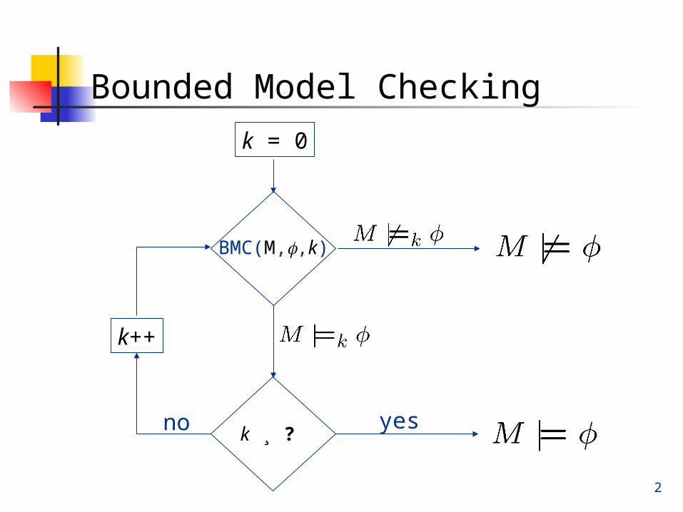
Bounded Model Checking
k = 0
BMC(M,,k)
yes
k++
k ¸ ?no

3
How big should k be?
For every model M and LTL property there exists k s.t.
M ²k ! M ²
We call the minimal such k the Completeness Threshold (CT)
Clearly if M ² then CT = 0 Conclusion: computing CT is at least as hard as
model checking
4
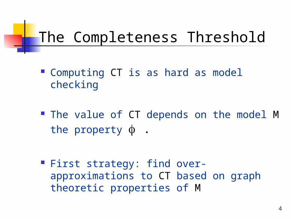
The Completeness Threshold
Computing CT is as hard as model checking
The value of CT depends on the model M
the property .
First strategy: find over-approximations to CT based on graph theoretic properties of M

5
Diameter d(M) = longest shortest path between any two reachable states.
Recurrence Diameter rd(M) = longest loop-free path between any two reachable states.
d(M) = 2
rd(M) = 3
Initialized Diameter dI(M) Initialized Recurrence Diameter rdI(M)
Basic notions…

6
The Completeness Threshold
Theorem: for p properties CT = d(M)
s0
p
Arbitrary path
Theorem: for }p properties CT= rd(M)+1
s0
ppppp
Theorem: for an LTL property CT = ?

8
LTL model checking
Given M,, construct a Buchi automaton B
LTL model checking: is : M £ B empty?
Emptiness checking: is there a path to a loop with an accepting state ?s0
9
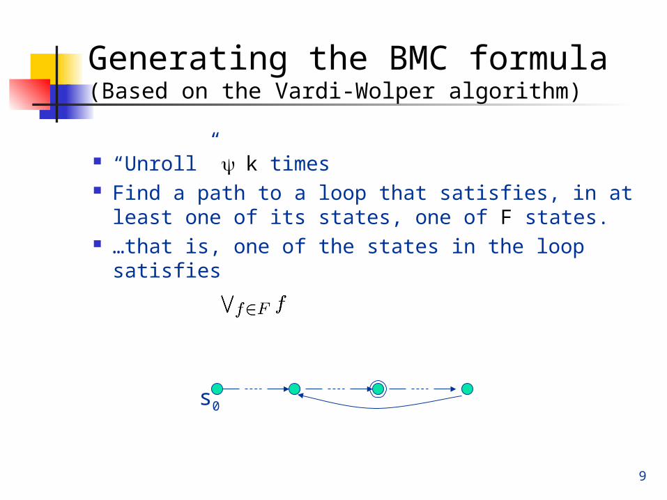
“Unroll” k times Find a path to a loop that satisfies, in at least
one of its states, one of F states. …that is, one of the states in the loop satisfies
s0
Generating the BMC formula(Based on the Vardi-Wolper algorithm)

10s0
Generating the BMC formula
Initial state:
k transitions:
Closing a cycle with an accepting state:
sksl
One of the states in the loop
Satisfies one of F states
Closing the loop

11
Completeness Threshold for LTL
It cannot be longer than rdI()+1 It cannot be longer than dI() + d() Result: min(rdI()+1, dI() + d())
s0

12
CT: examples
dI() + d() = 6rdI() + 1= 4
dI() + d() = 2rdI() + 1= 4 s0
s0

13
Computing CT (diameter) Computing d() symbolically with QBF: find
minimal k s.t. for all i,j, if j is reachable from i, it is reachable in k or less steps.
k-long path s0 -- sk+1
Complexity: 2-exp
k+1-long path s0 -- sk+1

14
Computing CT (diameter)
Computing d() explicitly: Generate the graph Find shortest paths (O||3) (‘Floyd-Warshall’ algorithm)
Find longest among all shortest paths
O(||3) exp3 in the size of the representation of
Why is there a complexity gap (2-exp Vs. exp3)? QBF tries in the worst case all paths between every
two states.
Unlike Floyd-Warshall, QBF does not use transitivity information like:

15
Computing CT (recurrence diameter)
Finding the longest loop-free path in a graph is NP- complete in the size of the graph.
The graph can be exponential in the number of variables.
Conclusion: in practice computing the recurrence diameter is 2-exp in the no. of variables.
Computing rd(y) symbolically with SAT. Find largest k that satisfies:
16
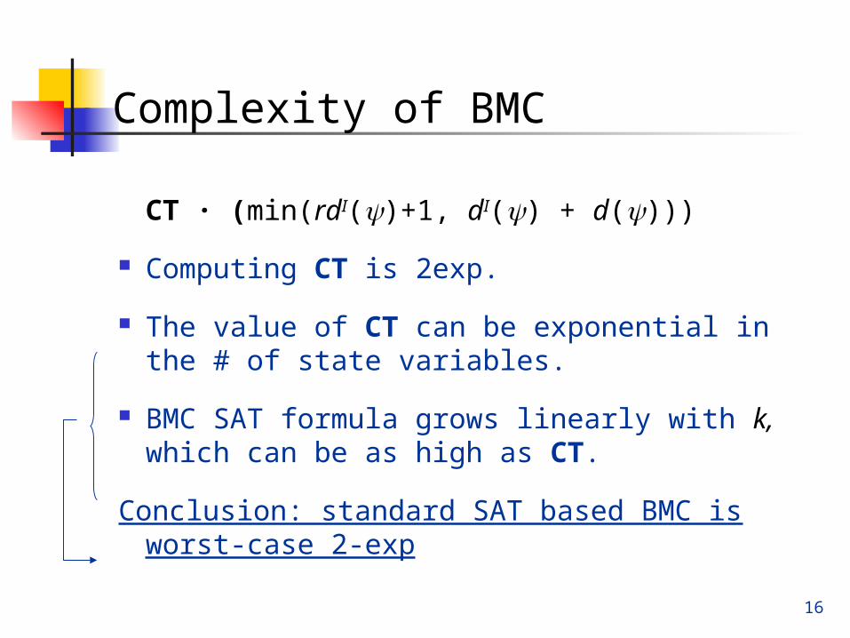
Complexity of BMC
CT · (min(rdI()+1, dI() + d()))
Computing CT is 2exp.
The value of CT can be exponential in the # of state variables.
BMC SAT formula grows linearly with k, which can be as high as CT.
Conclusion: standard SAT based BMC is worst-case 2-exp
17
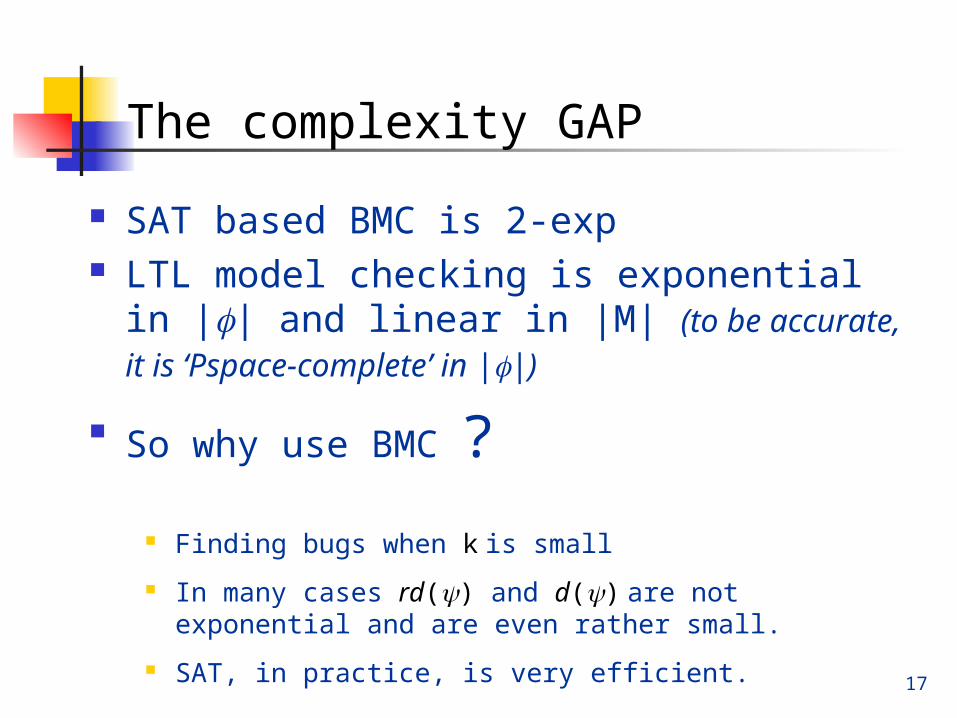
The complexity GAP
SAT based BMC is 2-exp LTL model checking is exponential in ||
and linear in |M| (to be accurate, it is ‘Pspace-complete’ in ||)
So why use BMC ?
Finding bugs when k is small
In many cases rd() and d() are not exponential and are even rather small.
SAT, in practice, is very efficient.

18
Closing the complexity gap
Why is there a complexity gap ? LTL-MC with 2-dfs :
dfs1
dfs2
Every state is visited not more than twice
19
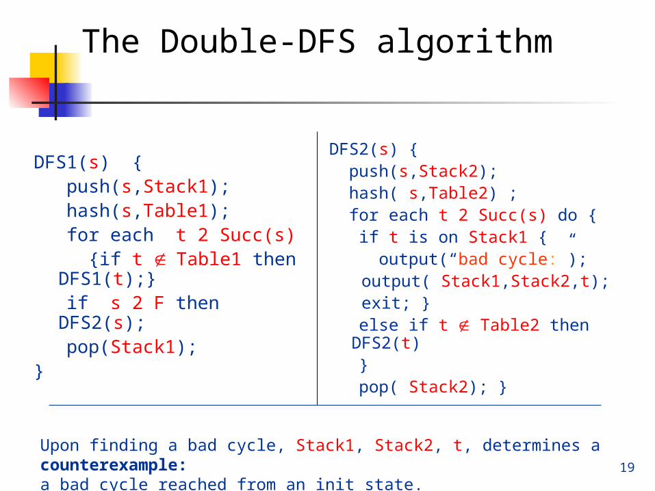
The Double-DFS algorithm
DFS1(s) { push(s,Stack1); hash(s,Table1); for each t 2 Succ (s) {if t Table1 then
DFS1(t);} if s 2 F then DFS2(s); pop(Stack1); }
DFS2(s) { push(s,Stack2); hash( s,Table2) ; for each t 2 Succ (s) do { if t is on Stack1 { output(“bad cycle:”);
output( Stack1,Stack2,t); exit; }
else if t Table2 then DFS2(t)
} pop( Stack2); }
Upon finding a bad cycle, Stack1, Stack2, t, determines a counterexample: a bad cycle reached from an init state.

20
Closing the complexity gap
2-dfs Each state is visited not more than twice
SAT Each state can potentially be visited an exponential
no. of times, because all paths are explored.

21
Closing the complexity gap (for p)
Force a static order, following a forward traversal
Each time a state i is fully evaluated (assigned): Prevent the search from revisiting it through deeper
paths
e.g. If (xi Æ :yi) is a visited state, then for i < j · CT add the following state clause: (:xjÇ yj)
When backtracking from state i, prevent the search from revisiting it in step i (add (: xi Ç yi)).
If :pi holds stop and return “Counterexample found”

24
Closing the complexity gap
Is restricted SAT better or worse than BMC ? Bad news:
We gave up the main power of SAT: dynamic splitting heuristics.
We may generate an exponential no. of added constraints
Good news Single exp. instead of double exp. No need to compute CT. (Instead of pre-computing
CT we can maintain a list of states and add their negation ‘when needed’).

25
Closing the complexity gap
Is restricted SAT better or worse than explicit LTL-MC ?
Not clear ! Unlike dfs, SAT has heuristics for
progressing. SAT has pruning ability of sets of states
26
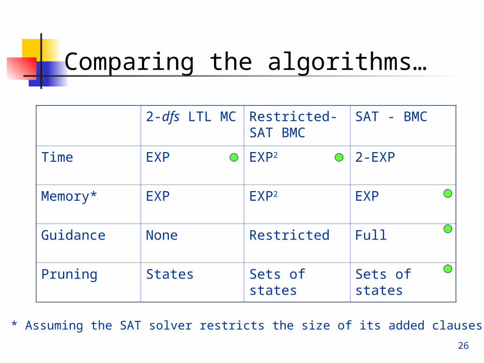
Comparing the algorithms…
2-dfs LTL MC Restricted-SAT BMC
SAT - BMC
Time EXP EXP2 2-EXP
Memory* EXP EXP2 EXP
Guidance None Restricted Full
Pruning States Sets of states Sets of states
* Assuming the SAT solver restricts the size of its added clauses