COMPLETE THERMAL DESIGN AND MODELING FOR THE...
182
COMPLETE THERMAL DESIGN AND MODELING FOR THE PRESSURE VESSEL OF AN OCEAN TURBINE – A NUMERICAL SIMULATION AND OPTIMIZATION APPROACH by Khaled Kaiser A Thesis Submitted to the Faculty of The College of Engineering and Computer Science in Partial Fulfillment of the Requirements for the Degree of Master of Science Florida Atlantic University Boca Raton, Florida December 2009
Transcript of COMPLETE THERMAL DESIGN AND MODELING FOR THE...

COMPLETE THERMAL DESIGN AND MODELING FOR THE PRESSURE
VESSEL OF AN OCEAN TURBINE – A NUMERICAL SIMULATION AND
OPTIMIZATION APPROACH
by
Khaled Kaiser
A Thesis Submitted to the Faculty of
The College of Engineering and Computer Science
in Partial Fulfillment of the Requirements for the Degree of
Master of Science
Florida Atlantic University
Boca Raton, Florida
December 2009


iii
ACKNOWLEDGEMENT
I have been working for this thesis for the last two years. Over the last two years, I have
benefited from the direct supervision of my thesis advisor Dr. Nikolaos Xiros. Without
his prudent and knowledgeable supervision, this thesis would not have seen the light of
publication. So, my first gratitude goes to my thesis advisor Dr. Xiros. Also over the
years, I have benefited form feedback and suggestions from the other two members of my
supervisory committee, Dr. Pierre-Philippe Beaujean and Dr. Frederick Driscoll. My
heartfelt gratitude and special thanks go to them. Unfortunately, space limitations do not
allow me to name everyone who has contributed. However, I wish to particularly thank
Dr. David Vendittis for his constructive suggestions.
I want to single out two others for special acknowledgement. Mustapha Mjit and Mico
Pajovic, two graduate students at FAU, their mental support and friendly behavior
motivated me to devote more time in research. I also want to thank Michael Seibert,
another graduate student, for playing a critical role in the development of this thesis.

iv
ABSTRACT
Author: Khaled Kaiser
Title: Complete Thermal Design and Modeling for the Pressure Vessel of An Ocean Turbine – A Numerical Simulation and Optimization Approach Institution: Florida Atlantic University
Thesis Advisor: Dr. Nikolaos Xiros
Degree: Master of Science
Year: 2009
This thesis is an approach of numerical optimization of thermal design of the
ocean turbine developed by the Centre of Ocean Energy and Technology (COET). The
technique used here is the integrated method of finite element analysis (FEA) of heat
transfer, artificial neural network (ANN) and genetic algorithm (GA) for optimization
purposes.

DEDICATED TO
MY PARENTS
FOR THEIR UNCONDITIONAL AND FOREVER LOVE

vi
COMPLETE THERMAL DESIGN AND MODELING FOR THE PRESSURE VESSEL OF AN OCEAN TURBINE – A NUMERICAL SIMULATION AND OPTIMIZATION
APPROACH
LIST OF FIGURES ............................................................................................................ x
LIST OF TABLES ........................................................................................................... xiii
CHAPTER 1 ....................................................................................................................... 1
1.1 Introduction ............................................................................................................... 1
1.2 Literature Review...................................................................................................... 2
1.2.1 ANN Application in Thermal Engineering ....................................................... 3
1.2.2 GA Application in Thermal Engineering .......................................................... 4
1.3 Objective and Scope of the Present Thesis ............................................................... 6
1.4 Thesis Organization .................................................................................................. 7
CHAPTER 2 ....................................................................................................................... 9
2.1 Chapter Introduction ................................................................................................. 9
PART-I Theoretical Background ......................................................................... 10
2.2 Modeling of Heat Conduction ................................................................................ 10
2.3 Initial and Boundary Condition .............................................................................. 12
2.4 Finite Element Approximating Functions in Two Dimensions .............................. 14
2.5 Two Dimensional Problem Solved using an Assembly of Elements ..................... 16
2.5.1 The use of Four-noded Rectangular Elements ................................................ 17
2.6 Time Stepping Methods for Heat Transfer ……….………………………………23

vii
2.6.1 Finite element time stepping ........................................................................... 23
2.6.1.1 Weighted Residual Method.................................................................. 24
2.6.1.2 Least Squares Method ......................................................................... 25
2.7 Nonlinear Heat Conduction Analysis ..................................................................... 26
2.7.1 Application of Galerkin’s Method to nonlinear transient heat conduction
problems ........................................................................................................ 26
PART - II Finite Element Analysis of Heat Transfer Using ANSYS ……………29
2.8 Analysis Considerations.......................................................................................... 29
2.9 Describing the geometry ......................................................................................... 30
2.10 Meshing................................................................................................................. 32
2.11 Axisymmetric analysis .......................................................................................... 32
2.12 Initial and boundary conditions ............................................................................ 34
2.13 ANSYS Results ..................................................................................................... 34
2.14 Fin Solution ........................................................................................................... 34
2.15 Chapter Summary ................................................................................................. 37
CHAPTER 3 ..................................................................................................................... 39
3.1 Introduction ............................................................................................................. 39
3.2 Artificial Neural Network: .................................................................................... 40
3.2.1 Neuron Model: ................................................................................................ 41
3.3 The Network Architecture ...................................................................................... 45
3.3.1 A Layer of Neurons ........................................................................................ 46
3.3.2 Learning Rules ………………………………………………………………50

viii
3.4 Separation of Data for Training and Testing and Network Performance ................... 50
3.5 Postprocessing the Data .......................................................................................... 61
3.6 Improving Generalization (Validation stop) ........................................................... 62
3.7 Summary ................................................................................................................. 65
CHAPTER 4 ..................................................................................................................... 67
4.1 Maximum temperature Analysis using Neural Network ........................................ 67
4.1.1 Network architecture ....................................................................................... 67
4.1.2 Training ........................................................................................................... 72
4.1.3 Network performance ..................................................................................... 73
4.1.4 Separation of data for training and testing ...................................................... 74
4.2 Artificial neural network results ............................................................................. 75
4.3 Error sources in ANN estimation ............................................................................ 79
4.4 Summary ................................................................................................................. 81
CHAPTER 5 ..................................................................................................................... 83
5.1 Introduction ............................................................................................................. 83
5.2 Basic Optimization Terminology ............................................................................ 84
5.3 Types of Optimization Problem .............................................................................. 85
5.4 How Genetic Algorithms Work .............................................................................. 86
5.5 The Numerical Design Optimization Problem ....................................................... 90
5.6 Thermal Design Optimization with genetic algorithm ........................................... 92
5.6.1 Genetic Algorithm (GA) Architecture ............................................................ 93

ix
5.7 Thermal Design Application domain: Motor-gear box arrangement domain
inside pressure vessel of an ocean turbine ............................................................. 97
5.7.1 Domain description ......................................................................................... 97
5.7.2 Dividing the domain ....................................................................................... 99
5.8 Genetic Algorithm Flowchart ............................................................................... 102
5.9 Optimum Results Obtained with Genetic Algorithm: .......................................... 103
5.10 Chapter Summary ............................................................................................... 105
CHAPTER 6 ................................................................................................................... 108
6.1 Summary of Benefits and Limitations for the Present Methodologies ................. 108
6.2 Conclusions ........................................................................................................... 110
6.3 Limitations and future work .................................................................................. 112
6.3.1 Limitations .................................................................................................... 112
6.3.2 Future works ................................................................................................. 113
APPENDIX A ................................................................................................................. 116
APPENDIX B ................................................................................................................. 129
APPENDIX C ................................................................................................................. 138
BIBLIOGRAPHY ........................................................................................................... 159

LIST OF FIGURES
Figure 1-1: The arrangement of the ocean turbine power plant ......................................... 7
Figure 2-1: General domain and boundary ....................................................................... 13
Figure 2-2: Node numbering for two-dimensional problem using linear elements .......... 15
Figure 2-3: Discretisation of a domain using four-noded rectangular elements ............... 18
Figure 2-4: A typical rectangular element e with local and global node numbers ........... 18
Figure 2-5: The geometric model for the 2D analysis showing all the areas ................... 31
Figure 2-6: Meshing of the design domain ....................................................................... 32
Figure 2-7: Axisymmetric ANSYS model ........................................................................ 33
Figure 2-8: Temperature distribution (2D) after 24 hours (in K0 ) without any fin ........ 35
Figure 2-9: Final temperature distribution (3D) after 24 hours (temp are in K0 ) ........... 36
Figure 2-10 : Final temperature distribution with five tin fins (temps are in K) .............. 37
Figure 3-1: Typical Neural Network ................................................................................. 41
Figure 3-2: Single-Input Neuron ....................................................................................... 42
Figure 3-3: Simple neuron with vector input .................................................................... 43
Figure 3-4: Log-Sigmoid Transfer Function..................................................................... 44
Figure 3-5: Layers of S Neurons ....................................................................................... 46
Figure 3-6: Three (hidden)-Layer Network ...................................................................... 49
x

xi
Figure 3-7: ANN prediction error vs. percentage of data used ......................................... 56
Figure 3-8: Standard Deviation Vs. % of data used .......................................................... 56
Figure 3-9: Testing of the NN with same set of training data from 10% to 40% ............. 57
Figure 3-10: Testing of the NN with the leftout data ranging from 10% to 40% ............. 57
Figure 3-11: Testing of the NN (trained with 10% - 40% data) with the total data ......... 58
Figure 3-12: Testing of the NN with same set of training data from 40% to 70% ........... 58
Figure 3-13: Testing of the NN with the leftout data ranging from 40% to 70% ............. 59
Figure 3-14: Testing of the NN (trained with 40% - 70% data) with the total data ......... 59
Figure 3-15: Testing of the NN with same set of training data from 70% to 99% ........... 60
Figure 3-16: Testing of the NN with the leftout data ranging from 70% to 99% ............. 60
Figure 3-17: Testing of the NN (trained with 80% - 99% data) with the total data ......... 61
Figure 3-18: Post regression of the trained Neural Network ............................................ 63
Figure 3-19: Typical training session of a Neural Network ............................................. 64
Figure 4-1: Network Responses of Architectures (a-top left corner) 5-10-1, (b-top right corner) 5-15-1, (c-bottom left corner) 5-17-1, and (d-bottom right corner) 5-10-10-1 .........................................................................................69
Figure 4-2: Network Responses of Architectures (a-top left corner) 5-15-10-1, (b-top
right corner) 5-15-14-1, (c-bottom left corner) 5-15-17-1, and (d-bottom right corner) 5-17-10-1 ..................................................................................69
Figure 4-3 : Network Responses of Architectures (a-top left corner) 5-17-14-1, (b-top
right corner) 5-10-10-10-1, (c-bottom left corner) 5-14-14-17-1, and (d-bottom right corner) 5-17-14-14-1 ................................................................70
Figure 4-4: Network Responses of Architectures (a-top left corner) 5-15-10-10-1, (b-
top right corner) 5-17-10-10-1, (c-bottom left corner) 5-17-10-14-1, and (d-bottom right corner) 5-17-14-10-1 ............................................................70
Figure 4-5:Configuration of a 5-17-14-14-1 neural network for maximum
temperature prediction ...................................................................................74
xii
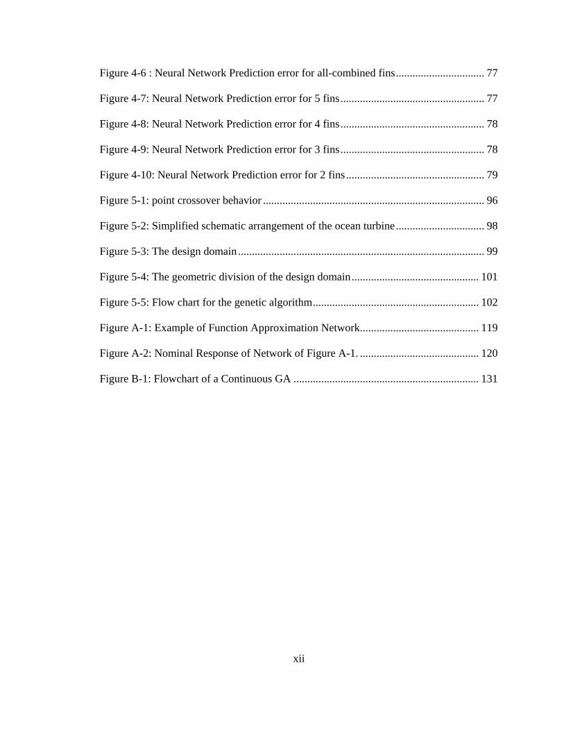
Figure 4-6 : Neural Network Prediction error for all-combined fins ................................ 77
Figure 4-7: Neural Network Prediction error for 5 fins .................................................... 77
Figure 4-8: Neural Network Prediction error for 4 fins .................................................... 78
Figure 4-9: Neural Network Prediction error for 3 fins .................................................... 78
Figure 4-10: Neural Network Prediction error for 2 fins .................................................. 79
Figure 5-1: point crossover behavior ................................................................................ 96
Figure 5-2: Simplified schematic arrangement of the ocean turbine ................................ 98
Figure 5-3: The design domain ......................................................................................... 99
Figure 5-4: The geometric division of the design domain .............................................. 101
Figure 5-5: Flow chart for the genetic algorithm ............................................................ 102
Figure A-1: Example of Function Approximation Network........................................... 119
Figure A-2: Nominal Response of Network of Figure A-1. ........................................... 120
Figure B-1: Flowchart of a Continuous GA ................................................................... 131

xiii
LIST OF TABLES Table 1-1: The estimated heat loss of the 20KW motor/generator ..................................... 2
Table 3-1: Standard deviation and maximum error for different % of data used ............. 54
Table 3-2: Mean error for different % of Data used ......................................................... 55
Table 4-1: Comparison of Results Obtained for Different Network Architectures .......... 72
Table 4-2: Network result for all fins combined ............................................................... 75
Table 4-3: Network results for different no of fins with different architectures .............. 76
Table 5-1: Comparison of GA results with ANSYS results ........................................... 104

1
CHAPTER 1 GENERAL INTRODUCTION
1.1 Introduction
The 20 KW ocean energy turbine created by the Center of Ocean Energy and
Technology (COET) at FAU is designed to generate energy out of a three-blade
propeller connected to an induction electric motor/generator through a shaft supported by
needle bearing and planetary gear reduction box. A motor driving a load is an energy
balanced system. On one side is the mechanical demand of the rotating load. On the other
is waste heat the motor generates turning that load. A small-sized motor that can not
dissipate waste heat fast enough rapidly burns out. Motors sized too large stay cool but
waste energy and money in inefficient operation. This waste heat can be dissipated using
heat sinks. According to the vibration theory, the location of heat sinks (fins) will give a
larger influence on the stress (strain) of fin joint under vibration. That is, the locations of
the fins are important factors to the reliability of the whole system. So, it is of particular
interest from the point of safety and Machinery Condition Monitoring (MCM) to
dissipate this amount of heat so that the motor/generator and the other electronic
components inside the pressure vessel keep working under their safe operating
temperature. This can be done by selecting the optimal design for heat dissipation.
For doing this the technology applied here is the Finite Element Method (FEM) in heat
transfer and numerical optimization.
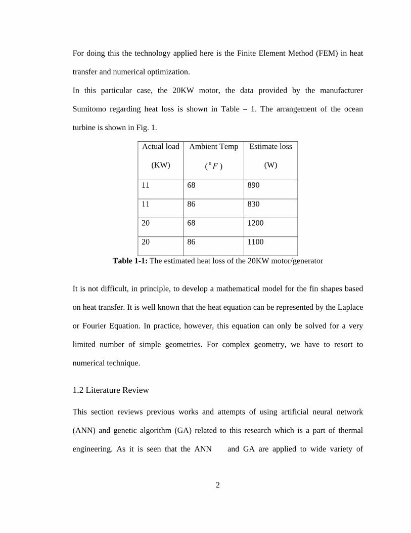
In this particular case, the 20KW motor, the data provided by the manufacturer
Sumitomo regarding heat loss is shown in Table – 1. The arrangement of the ocean
turbine is shown in Fig. 1.
Actual load
(KW)
Ambient Temp
( ) 0 F
Estimate loss
(W)
11 68 890
11 86 830
20 68 1200
20 86 1100
Table 1-1: The estimated heat loss of the 20KW motor/generator
It is not difficult, in principle, to develop a mathematical model for the fin shapes based
on heat transfer. It is well known that the heat equation can be represented by the Laplace
or Fourier Equation. In practice, however, this equation can only be solved for a very
limited number of simple geometries. For complex geometry, we have to resort to
numerical technique.
1.2 Literature Review
This section reviews previous works and attempts of using artificial neural network
(ANN) and genetic algorithm (GA) related to this research which is a part of thermal
engineering. As it is seen that the ANN and GA are applied to wide variety of
2

3
thermal engineering, encourages us to apply ANN and GA in our design problem.
1.2.1 ANN Application in Thermal Engineering
In the past, applications of ANN to engineering problems have been attempted in
structural engineering and engineering mechanics (Zeng, 1998). Tentative studies of
applying ANN to problems in thermal systems have been carried out quite recently, with
a relatively short history. With the exception of neural networks and control systems
applied to heating, ventilating, and air-conditioning systems, the studies have been
somewhat sporadic and in only some distinct areas of application. For heat transfer data
analysis and correlation, an ANN- based methodology was proposed by Thibault and
Grandjean (1991) and a similar methodology was introduced by Jambunathan et al.
(1996) to predict coefficients of heat transfer in convective-flow systems using liquid
crystal thermography. Both steady and unsteady heat conduction problems were treated
by ANN in studies by Gobovic and Zaghloul (1993), Yentis and Zaghloul (1994), and
Kuroe and Kimura (1995). Kaminski et al. (1996) gave an interesting description of the
thermal deterioration process based on combined ANN and GA analysis. An ANN was
also used to identify location and strength of unknown heat sources by sparse temperature
measurements (Momose et al., 1993). In addition, an ANN-based attempt was made to
predict measured intrinsic thermodynamic properties (Normandin et al., 1993).
ANN analyses have also been utilized to study and predict the performance of specific
thermal devices and systems. Good estimates of the thermal storage loads and the
dynamic system operation of typical thermal storage systems were obtained by Ferrano
and Wong (1990) and Ito et al. (1995). Heat exchanger performance and control
were studied by Diaz et al. (1996, 1998, 1999), Lavric et al. (1993, 1994), and Bittanti

4
and Piroddi (1997). Several industrial applications of ANN were also demonstrated, in a
fluidized- bed dryer (Zbicinski et al., 1996), in a liquid-sodium reflux-pool boiler solar
receiver (Fowler et al., 1997), in a steel annealing furnace (Pican et al., 1998), and in the
design of a chemical injection-system retrofit fuzzy control system in a thermal power
plant (Moon and Cho, 1996). Other specific applications include manufacturing and
materials processing involving microelectronic manufacturing (Mahajan and Wang,
1993), a coordinate grinder (Yang et al., 1995), rapid thermal processing control (Fortuna
et al., 1996), sensors and sensor analysis involving thermal image processing (Naka et al.,
1993), and blast furnace probe temperatures (Bulsari and Saxin, 1995).
Kawashima et al. (1995) did a 24-h thermal load prediction. Li et al. (1996) developed a
fault diagnosis method for heating systems using neural networks. Matsumoto et al.
(1996, 1997) studied the effect of pin fin arrangement on endwall heat transfer.
All the studies mentioned above represent tentative attempts to apply the ANN analysis
to thermal system problems. Since good results have been obtained so far, there is no
reason to expect that the ANN approach cannot be applied to many other thermal
problems with equal success, particularly in the analysis of dynamic systems and their
control.
1.2.2 GA Application in Thermal Engineering
Though the GA is a relatively new technique in relation to its application to thermal
engineering, there are a number of different applications that have already been
successful. Davalos and Rubinsky (1996) adopted an evolutionary-genetic approach for
numerical heat-transfer computations. Shape optimization is another area that
has been developed. Fabbri (1997) used a GA to determine the optimum shape of a fin.

5
The placing of electronic components as heat sources is a problem that has become very
important recently from the point of view of computers. Queipo et al. (1994) applied GAs
to the optimized cooling of electronic components. Tang and Carothers (1996) showed
that the GA worked better than some other methods for the optimum placement of chips.
Queipo and Gil (1997) worked on the multiobjective optimization of component
placement and presented a solution methodology for the collocation of convectively and
conductively air-cooled electronic components on planar printed wiring boards. Mey senc
et al. (1997) studied the optimization of microchannels for the cooling of high-power
transistors. Inverse problems may also involve the optimization of the solution. Allred
and Kelly (1992) modified the GA for extracting thermal profiles from infrared image
data which can be useful for the detection of malfunctioning electronic components.
The two-dimensional temperature distribution for a given fin shape was found using a
finite-element method. The fin shape was proposed as a polynomial, the coefficients of
which have to be calculated. The fin was optimized for polynomials of degree 1 through
5. Von Wolfersdorf et al. (1997) did shape optimization of cooling channels using GAs.
The design procedure is inherently an optimization process. Androulakis and
Venkatasubramanian (1991) developed a methodology for design and optimization that
was applied to heat exchanger networks; the proposed algorithm was able to local
solutions where gradient-based methods failed. Abdel-Magid and Dawoud (1995)
optimized the parameters of an integral and a proportional-plus-integral controller of a
reheat thermal system with GAs. The fact that the GAs can be used to optimize in the
presence of variables that take on discrete values was put to advantage by Schmit et al.
(1996) who used it for the design of a compact high-intensity cooler.

6
Jones et al. (1995) used thermal tomographic methods for the detection of
inhomogeneities in materials by finding local variations in the thermal conductivity.
Rauden- sky et al. (1995) used the GA in the solution of inverse heat conduction
problems. Okamoto et al. (1996) reconstructed a three-dimensional density distribution
from limited projection images with the GA. Wood (1996) studied an inverse thermal
field problem based on noisy measurements and compared a GA and the sequential
function specification method. Li and Yang (1997) used a GA for inverse radiation
problems. Castrogiovanni and Sforza (1996, 1997) studied high-heat flux-flow boiling
systems using a numerical method in which the boiling-induced turbulent eddy
diffusivity term was used with an adaptive GA closure scheme to predict the partial
nucleate boiling regime.
1.3 Objective and Scope of the Present Thesis
The overall objective of the present thesis is to provide methodologies that allow accurate
estimation of the heat transfer rate inside the pressure vessel domain of the ocean turbine
shown in Figure-1 for the analysis, design and control of thermal systems. To achieve
such a goal, this study has made use of techniques that belong to the areas of optimization
and artificial/computational intelligence; in particular finite element analysis, genetic
algorithms and artificial neural networks. The procedure developed on the basis of the
aforementioned methods has been applied to a pressure vessel of the ocean turbine for the
purpose of machinery condition monitoring, health prognostics and diagnostics. The
procedure can be used as a design tool for different geometrical complexities and other
decision variables. The optimization algorithm and the objective function used

here have left rooms for other design variables than the variables considered here. In
general, in can be a very useful design tool for this type of ocean energy industry.
The importance of this investigation is that it will provide both the motor and the thermal
system engineer with appropriate tools to accurately simulate the heat transfer
characteristics of an ocean turbine for their design, as well as their analysis and selection.
Figure 1-1: The arrangement of the ocean turbine power plant (Courtesy of Dr. Driscoll,
COET at FAU)
1.4 Thesis Organization
This thesis focuses on the numerical optimization of thermal design of the pressure vessel
of an ocean turbine. The aim of this thesis is to highlight the main parameters of the
thermal design process and thus its optimal conditions of use. The thesis is organized in
six main chapters:
7
Chapter 1, dedicated to the general introduction of the methodology, introduces the
problem statement. This chapter reviews the literature, and describes the objective of the
thesis.

8
Chapter 2 describes in a nutshell the finite element approach of the design process and
describes the design domain. Part-I describes the modeling of heat equation and the initial
and boundary conditions, and also various formulations for various discretization
methods. Part-II describes the ANSYS simulation of heat transfer for the present
problem.
Chapter 3 presents the neural network analysis of heat transfer. Starting with the basic
ideas of neural network, this chapter goes deep into the neural network architecture for
the specific type of problem considered in this thesis.
Chapter 4 presents the artificial neural network analysis of the present problem. This is
the continuation of the previous chapter. This chapter describes the methodology for the
chosen architecture of the network and describes the results obtained form the network.
Chapter 5 is dedicated to the genetic algorithm for the design optimization. This chapter
delves into the design process for exploring the solution field for the optimum results.
This chapter also describes the nonlinear objective function obtained from the previous
chapter’s ANN.
And finally Chapter 6 concludes with a summary of the thesis, includes the limitations of
this thesis and suggests the scope of future research.

9
CHAPTER 2 FINITE ELEMENT ANALYSIS OF HEAT TRASNFER
2.1 Chapter Introduction
Over the past three decades, the use of numerical simulation with high-speed computers
has gained wide acceptance throughout most of the major branches of engineering. There
are many practical engineering problems that require the analysis of problems involving
the transfer of heat. The solution of the equation of heat conduction is sufficient in many
cases; in other cases the numerical simulation of the process can prove to be extremely
useful.
In the field of design engineering, there are numerous examples of practical problems
where the behavior of the system under consideration may be predicted via a heat transfer
analysis. Mathematical models, which can accurately predict the heat transfer behavior,
are often the only means of gaining a better insight into the physical process. If the
numerical method makes accurate predictions of the problem, the numerical results can
also be used to aid the design of the optimal arrangement.
Exact analytical solutions of the governing equations of heat transfer can only be
obtained for problems in which restrictive simplifying assumptions have been made with
respect to geometry, material properties and boundary conditions. There is therefore no
option but to turn to numerical solution methods for the analysis of practical
problems, where such simplifications are not generally possible. The finite element
method, with its flexibility in dealing with complex geometries, is an ideal approach to
employ in the solution of such problems.
In the first part of this chapter we first describe briefly the basic theories and governing
equations of finite element analysis of heat transfer and then in the second part we
present the numerical model analysis of the present problem in ANSYS and shows the
result.
PART-I Theoretical background
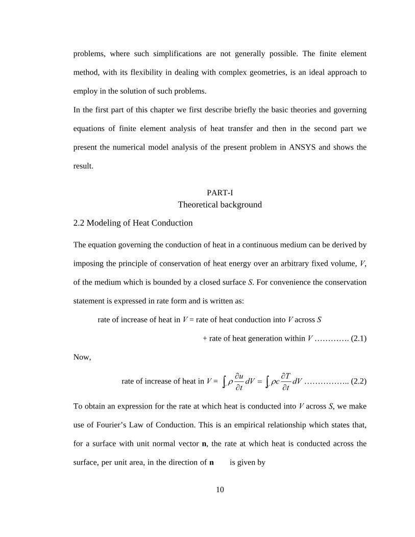
2.2 Modeling of Heat Conduction
The equation governing the conduction of heat in a continuous medium can be derived by
imposing the principle of conservation of heat energy over an arbitrary fixed volume, V,
of the medium which is bounded by a closed surface S. For convenience the conservation
statement is expressed in rate form and is written as:
rate of increase of heat in V = rate of heat conduction into V across S
+ rate of heat generation within V …………. (2.1)
Now,
rate of increase of heat in V = ∫∫ ∂∂
=∂∂
VVdV
tTcdV
tu ρρ …………….. (2.2)
To obtain an expression for the rate at which heat is conducted into V across S, we make
use of Fourier’s Law of Conduction. This is an empirical relationship which states that,
for a surface with unit normal vector n, the rate at which heat is conducted across the
surface, per unit area, in the direction of n is given by
10

nTkTkq∂∂
==−= n).grad( …………. (2.3)
Thus, if n denotes the outward unit normal to S, it follows that
rate of heat conduction into V across S
= …….. (2.4) dVTkdSTkqdSVSS
) grad (div.) grad( ∫∫∫ == n
where the Divergence Theorem has been applied.
If it is assumed that heat generation in the medium is occurring at a rate Q per unit
volume, then
rate of heat generation within V = ∫ ……………. (2.5) V
QdV
Using equations (2.2), (2.4) and (2.5) in (2.1) produces the conservation statement:
∫ =⎟⎠⎞
⎜⎝⎛ −
∂∂
V
dVQTktTc 0-) grad div(ρ ………………. (2.6)
and, since the volume V was arbitrarily chosen initially, it follows that
QTktTc +=∂∂ ) grad div(ρ …………………… (2.7)
everywhere in the medium. This is the familiar form of the heat conduction equation for a
non-stationary system.
where, u = specific internal energy of the medium
ρ = density of the medium
c = specific heat of the medium; dTduc =
T = temperature
11
k = thermal conductivity (property of the medium)

n∂∂ = differentiation in the direction of n
q = flux of heat in this direction
Q = rate of heat generation per unit volume
If the conductivity k and the specific heat capacity cρ are assumed to be constant, and if
the heat generation rate Q is independent of T, then equation (2.7) is linear and can be
written as
kQT
tT
+∇=∂∂ 2
1
1α
……………………… (2.8)
where c
kρ
α =1 is termed the thermal diffusivity of the medium and denotes the
Laplacian operator defined, in Cartesian Coordinates, by
2∇
2
2
2
2
2
22
zyx ∂∂
+∂∂
+∂∂
=∇ ……………………… (2.9)
2.3 Initial and Boundary Condition
The solution of heat conduction equation is required over an arbitrary domain Ω
bounded by a closed surface, Γ , as illustrated in Figure 2-1.
For the steady state heat conduction equation, one condition has to be specified at each
point of the boundary curve Γ and the typical conditions of practical interest would be:
a) the value of the temperature is prescribed, e.g. )(xfT = for all x on 1Γ ,
or
b) the value of the outward normal heat flux is
12

prescribed, e.g. ),(),(),(). grad( TTTnTkTkq rc xxxn ℵ+ℵ+ℵ=∂∂
−=−=
for all x on 2Γ .
Here are prescribed functions of x and T and rcf ℵℵℵ and , , 0 , 2121 =Γ∩ΓΓ∪Γ=Γ .
Ω
2Γ
n̂
1Γ
21 Γ∪Γ=Γ
Figure 2-1: General domain and boundary Here,
= specified heat flux ℵ
cℵ = convective heat flux = )( ∞−TTα
rℵ = radiative heat flux = )( 44∞−TTεσ
α = coefficient of surface heat transfer
∞T = specified ambient temperature
σ = Stefan-Boltzman constant
ε = emmisivity of the surface
13
For transient problem, the solution is uniquely determined provided that an

14
in
time, usually ta 0. In addition, in a
ient problem the functions
itial condition is given together with a boundary condition at each point of the boundary
Γ of the domain. The initial condition should give the distribution of the temperature over
the entire region Ω at an initial ken to be the time t =
trans , rcf ℵℵℵ and , , may vary with time.
solution to a two-dimensional heat
conduction problem on a square region defined by
2.4 Finite Element Approximating Functions in Two Dimensions
Now consider the construction of an approximate
1,1 0 <<−=+⎟⎟⎠
⎞⎜⎜⎝
⎛∂∂
∂∂
+⎟⎟⎠
⎞⎜⎜⎝
⎛∂∂
∂∂ ηξ
ηηξξQTkTk ……….. (2.10)
1on )( −== ηξfT ………………. (2.11)
1on and 1on =±=ℵ=∂∂
−= ηξn
kq ……………….. (2.12)
Here, Qfk and , , , ℵ are prescribed functions. If an approximate solution to this problem
is to be sought by applying the Galerkin procedure, a suitable polynomial approximating
function set can be obtained by direc onal f ment
ideas. We select a set 11 ,......, ,
T
t extension of the one-dimensi inite ele
of M+1 points 1+Mξξξ such that 11 −=ξ and 11 =+Mξ , and
a set of M+1 points 121 ,......., , +Mηηη , such that 11 −=η and 11 =+Mη . Nodes, numbered
so that the first 4M lie on the boundary and the first M+1 lie on the line 1−=η , as shown
in Figure 2.2, are located at the points ( )lk ηξ , and the associated Lagrange interpolation
polynomials )()( ξMkL and )()( ηM
lL are constructed. For node j, located at ( )lk ηξ , , the
finite element shape function is defined by
( ) )()(, )()( ηξηξ Mn
MkjN LL= ………….. (2.13)

15
all the other nodes. The
trial function set for these approximating functions becomes
This function has the value unity at node j and the value zero at
))1(( +MMT⎪⎭
⎪⎬⎫
⎪⎩
⎪⎨⎧
−===+== ∑∑++
+=
1)1(
21on ˆˆ ; ;ˆ|ˆ
2 MM
Mjjj fTNfNTTT ηψψ
=1jjj ………… (2.14)
Figure 2-2: Node numbering for two-dimensional problem using linear elements
and the corresponding weighting function set is
……………. (2.15)
that mbers
)M(M )1( +W⎪⎭⎪⎩ += 2Mj
Note now the nu
⎪⎬⎫⎪
⎨⎧
−==== ∑+
1on 0 ;|2)1(
ηWNbWWM
jj
T̂ of the trial function set satisfy on the
boundary
fT ˆˆ =
1−=η , where
3M-1 3M-2 2M+33M+1 3M 2M+4
ξ
η
M+2
M+3
M+4 4η
3η
2η
1η
2M-1
2M
2M+1 2M+2
1+Mη
Mη 3M+2
1−Mη3M+3
1+Mη3M+4 2M-2
4M-2
4M-1
4M
M M+1 M-1 M-2
2−Mξ 1−Mξ Mξ 1+Mξ1ξ 2ξ 3ξ 4ξ3 41 2

16
In this representation, denotes the value of
∑+
−1
)1,(ˆM
Nff ξ ………………. (2.16)
j
=
=1
)(j
jjξ
f )(ξf at node j, i.e. at jξξ = , and (2.16) is
which passes through the prescribed
values at the points
the Lagrange interpolating polynomial of degree M
1+M121 ,......, , +Mfff 21 ,....., , ξξξ .
2.5 Two Dimensional Problem Solved using an Assembly of Elements
Consider the problem of steady state heat conduction in a two-dimensional region,Ω ,
with closed boundary curve, Γ , and of thermal conductivity k. If heat is generated w
the region at a prescribed rate Q per unit area, then the distribution of temp
through is governed by the solution of the equation
ithin
erature
Ω
Ω=+⎥⎦
⎤⎢⎣
⎡∂∂
∂∂
+⎥⎦⎤
⎢⎣⎡ ∂∂
=+) grad (div TkQTk∂∂
in 0QyTk
yxx…….. (2.17)
subject to the general boundary conditions
1on for )( Γ= xxfT ………………………… (2.18)
2on for ). grad (-q Γ,T)(nTk xℵ=Tk xn∂∂
−==
recall that
………… (2.19)
We 0 , 2121 =Γ∩ΓΓ=Γ∪Γ and that ℵ ,f will be prescribed functions. The
can be achieved by appropriate definition
on and alues
application of particular boundary conditions
and the specification of the v1Γ 2Γ f and ℵ .

2.5.1 The use of Four-noded Rectangular Elements
Consider again the solution of the heat conduction problem defined by equations (2.17)-
(2.19), over the rectangular domainΩ defined by yx LyLx ≤≤≤≤ 0 ,0 . In this case, the
domain is subdivided to create a mesh of non-overlapping four-noded rectangular
elements, as shown in Figure 2-3. As before, the nodes and the elements are nu bered.
Figure 2-4 shows a typical element e with nodes which are locally numbered 1, 2, 3, 4
and which are globally numbered I, J, K, L. If the
m
th in the x
direction and of length in the l ent can be
mapped exactly into this element e by the mapping
element is of leng
ction, the standard square bilinear e
xeh
emyeh y dire
22),(
22),(
4
1
4
1
η
ξηξ
yeyeI
jjje
xexeI
jjje
hhyyxNyy
hhxNxx
++==
++==
∑
∑
=
=……………………………… (2.20)
Since IJyeIKL
ILxeIKJ
yyhyyyxxhxxx
=+===+==
……………… ………….. (2.21) …
17

18
Figure 2-3: Discretisation of a domain using four-noded rectangular elements
Figure 2-4: A typical rectangular element e with local and global node numbers
Over this element, we work with trial functions
22 24 23 25 21
13 14 15 16
16 20 1917 18
12 9 11 10
15 11 12 13 14
8 7 6 5
610 87 9
3 4 1 2 h
1 1 2 3 4 5
h
e
1 2
3 4L K
3
yeh 24
1
I J xeh
19
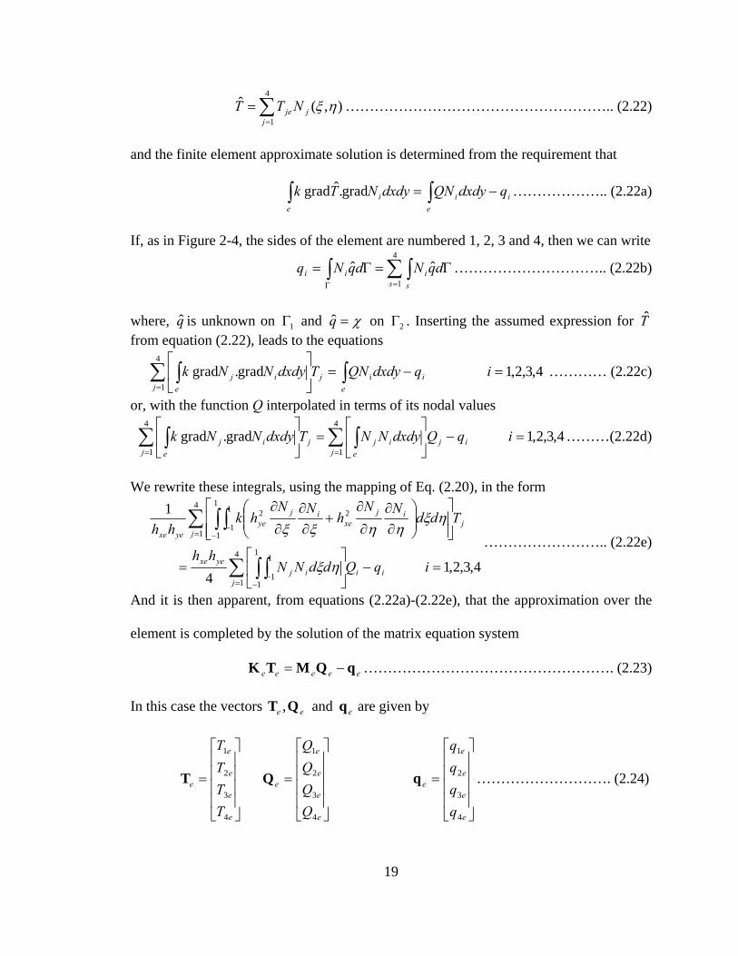
……………………………………………….. (2.22)
and the finite element approximate solution is determined from the requirement that
If, as in Figure 2-4, the sides of the element are numbered 1, 2, 3 and 4, then we can write
where, is unknown on and
∑=
=4
1),(ˆ
jjje NTT ηξ
iii qdxdyQNdxdyNTk −= ∫∫ grad.ˆgrad ……………….. (2.22a) ee
∑∫ Γ=Γ4
ˆdqN ………………………….. (2.22b) ∫=Γ
=1
ˆs s
iii dqNq
. Inserting the assumed expression for T̂ q̂ 1Γ χ=q̂ on 2Γfrom equation (2.22), leads to the equations
(2.22c)
or, with the function Q interpolated in terms of its nodal values
We rewrite these integrals, using the mapping of Eq. (2.20), in the form
4,3,2,1 d =iqQN ii …………gra.grad i
4
1−=⎥
⎦
⎤⎢⎣
⎡∫∑ ∫
=
dxdyNTdxdyNke
jj e
j
4,3,2,1 grad.grad =−⎥⎦
⎢⎣
=⎥⎦
⎢⎣
∑ ∫∑ ∫==
iqQdxdyNNTdxdyNNk ij
je
ijjj e
ij ………(2.22d) 4
1
4
1
⎤⎡⎤⎡
4,3,2,1 4
1
4
1
1
1
1
1
4
1
1
1
1
1
22
=−⎥⎦
⎤⎢⎣
⎡=
⎥⎥⎦
⎤
⎢⎢⎣
⎡⎟⎟⎠
⎞⎜⎜⎝
⎛∂∂
∂
∂+
∂∂
∂
∂
∑ ∫ ∫
∑ ∫ ∫
= −−
= −−
iqQddNNhh
TddNN
hNN
hkhh
iij
ijyexe
jj
ijxe
ijye
yexe
ηξ
ηξηηξξ
…………
And it is then apparent, from equations (2.22a)-(2.22e), that the approximation over the
element is completed by the solution of the matrix equation system
………….. (2.22e)
eeeee qQMTK −= ……………………………………………. (2.23)
In this case the vectors are given by eee qQT and ,
⎥⎥⎥⎥
⎢⎢⎢⎢
e
eT
3
2 ⎥⎥⎥⎥
⎢⎢⎢⎢
e
eQ
3
2
⎥⎥⎥⎥
⎢⎢⎢⎢
e
eq
3
2 ………………………. (2.24)
⎦
⎤
⎣
⎡
=
e
e
e
TT
T
4
1
T
⎦
⎤
⎣
⎡
=
e
e
e
Q
4
1
Q
⎦
⎤
⎣
⎡
=
e
e
e
q
4
1
q
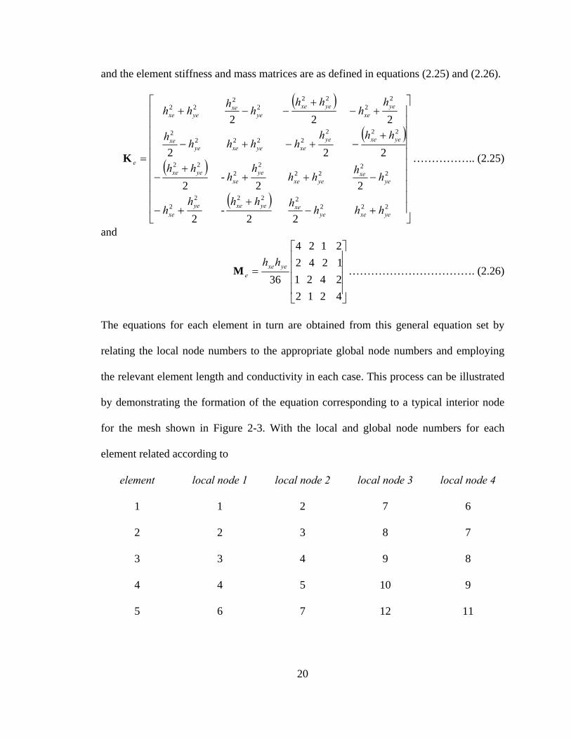
and the element stiffness and mass matrices are as defined in equations (2.25) and (2.26).
( )
( )
20
( )
( )⎥⎥⎥⎥⎥
⎥⎥⎥
⎦⎢⎢⎢⎢⎢
⎢
⎣+
++−
−++
−
+−−
+−−−+
222222
2
222
22
22
2222222
2
2
2
2
2
2
2
2
yexeyexeyexeye
xe
xeyexe
yexe
yexe
yexeyeye
xe
xeyeyexe
e
hhhhhhh
h
hh
hhhhh
hhhhh
h
hhhh
…… )
and
⎥⎥
2 …
⎤
⎢⎢
⎡ +
2
22
222
222
22yeyexexe hhhh
⎢⎢
=
K
−
+
+− 2
xeh+ xeye h
2
2ye
-
- h
…….. (2.25
⎥⎥⎥⎥
⎦
⎤
⎢⎢⎢⎢
⎣
⎡
=
4 2 1 22 4 2 11 2 22 1 2 4
36yexe
e
hhM ……………………………. (2.26)
The equations for each element in turn are this general equation
relating the local node numbers to the appropriate global node numbers and employing
the relevant element length and conductivity in each case. This process can be illustrated
by demonstrating the formation of the equation corresponding to a typical interior node
for the mesh shown in Figure 2-3. With the local and global node numbers for each
element related according to
element local node 1 local node 2 local node 3 local node 4
4
obtained from set by
1 1 2 7 6
2 2 3 8 7
3 3 4 9 8
4 4 5 10 9
5 6 7 12 11

21
6 7 8 13 12
7 8 9 14 13
8 9 10 15 14
. . . . .
. . . . .
. . . . .
we select node 7 as a typical interior node and note that it belong
, 2, 5 and 6. We therefore need to examine the element equation (2.23) for
each of these elements and identify the component corresponding to node 7 in each case.
Assuming that , the equations corresponding to node 7 can be seen to be
s to the four elements
numbered 1
hhh yexe ==
Element 1
[ ] )1(76721
26
72
11 242
3622
23qQQQQhT
TTTk−+++=⎥⎦
⎤⎢⎣⎡ −+−− ……………… (2.27a)
lement 2 E
[ ] )2(77832
2
78
322 4222 qQQQQhT
TTTk
−+++=⎥⎤
⎢⎡ +−−− ……………... (2.27b)
36223 ⎦⎣
Element 5
[ ] )5(7111276
2
1112
765 242
3622
23qQQQQhTTT
Tk−+++=⎥⎦
⎤⎢⎣⎡ −−+− ……………... (2.27c)
Element 6

[ )6(7121387
212
138
76 224
36222
3qQQQQhTT
TT
k−+++=⎥⎦
⎤⎢⎣⎡ −−− ]
equation for node 7 is obtained by adding these four equations
together and using the continuity of flux requirement to set
……………... (2.27d)
and the assembled
0)6(7)5(7)2(7)1(7 =+++ qqqq …………………………………………. (2.28)
This equation is valid provided that there is no source or sink of heat at this node.
Node 15 can be regarded as a typical node on the bounda
elements 8 and 12 only. Considering each of these elements in turn, we find that the
equations corresponding to node 15 are
ry and it can be seen to belong
to
From element 8:
[ ] )8(151415109159 361
223TTk
⎥⎦⎤
⎢⎣⎡
From element 12:
14108 2422 qQQQQTT −+++=−+−− ……………… (2.29a)
[201412 24212 QQQQTT
TTk+++=⎤⎡ −−+− ] )12(15192015141915 36223
q−⎥⎦⎢⎣…………… (2.29b)
Adding these two equations produces the assembled equation for node 15. we note that in
this case
∫ Γ= dNχ ………………………… (2.30) −+−
+)2015()1510( 15)12(15)8(15 qq
22

23
oblems can therefore be termed initial value problems. The
2.6 Time Stepping Methods for Heat Transfer
The majority of engineering problems are transient in nature and we are required to solve
the time-dependent equation, which yield the solution at various times. In addition to the
boundary conditions at any time, we are typically given the initial state of system, at
time 0=t . Transient pr
transient heat conduction problem is given by the equation
( ) QTktT∂c +=∂
grad divρ ……………………………………. (2.31)
al discretization yields the matrix equation system Application of the finite element spati
fKTTM =+& …………………………………………………. (2.32)
where M is the capacitance matrix, K is the conductance matrix and is the
temperature differentiated with respect to t
ua
ia
as partial discretisation.
Two techniques are employed to fully discretise the system of equations: the finite
difference method and the finite element method.
2.6.1 Finite element time stepping
In order to produce a finite element algorithm, we shall discretise the
T&
ime.
Although an analytical solution of (2.32) is possible for simplified, linear cases, it is more
usual for the system of ordinary differential eq tions to be discretised in time, from
which solutions at various times can be obtained. Since the original partial different l
equation becomes a discrete set of ordinary differential equations, the process is known

24
temperature in time by the normal finite element procedure, i.e.
∑= ii tN TT )( ………………………………………… (2.33)
The differential equation given by (2.31) is first order, with respect to the time derivative.
It is therefore only necessary to provide first-order (i.e. linear) shape functions, , in
me. It should also be noted at this stage that are assumed to be the sam
component of T and are therefore scalar. If the n perature values change from
)(tNi
e for each iN
odal tem nT
ti
to 1+nT over a time step of length tΔ , the shape functions are given by
ξξ =−= +1 1 nn NN …………………………….. (2.34)
where ξ is a local variable varying between 0 and 1 and is given by
ttΔ
=ξ
Hence the temporal derivatives of the shape functions are given by
tN
tN nn Δ
=Δ−
= + 1 ………………………… (2.35)
The problem can now be developed in two different ways. The weighted residual method
can be applied in the normal manner, or the error with respect to
11 &&
1+nT can be minimized
uce a least squares algorithm. We consider each of these methods in turn.
2.6.1.1 Weighted Residual Method
The discretisation of the equation system (2.32) in time produces
to prod
( ) ( ) fTTKTTM =+++ ++
++
11
11
nn
nn
nn
nn NNNN ………………….. (2.36)
Employing the usual weighted residual method in (2.36) then gives

( ) ([ ]1
011
1 +++∫ +++ NNN nn
nn
nn
n TKTTM ) 01 =−+ ξdNn fT …………… (2.37)
25
Substituting in the expressions for the shape functions, (2.34), and their derivatives,
(2.35), then leads to
fTKMM ˆ1 ⎞⎝⎛Δ⎠
⎞⎝⎛Δ
+ nn
tt
where
TK )1( +⎟⎠
⎜ −−=⎟⎜ + θθ ……………………….. (2.38)
∫
∫
∫
∫== 1
0
1
01
0j
1
0 ˆ ξ
ξ
ξ
ξξθ
dW
dW
dW
dW
j
jj ff
If the same spatial interpolation is used for both and , then is given by
………………………………….. (2.39)
2.6.1.2 Least Squares Method
A least squares algorithm is derived by utilizing a functional that minimizes the squares
] ……….. (2.40)
By noting that, for any of the vectors above, we can write
f T f̂
)1(ˆ −+= nn fff θθ 1+
of the error in the solution at the new time step, . Therefore, across each time step,
i.e. between n and n+1, we must minimize the functional
( ) ([π NNN nn
nn
nn
1
11∫ +++= ++ TKTTM &&
1+nT
) ξdNnn
2
01
1 −++ fT
XXX ⋅T 2 =
The resulting least squares scheme is given by

( )
( )
26
∫∫ −−⎥⎤
⎢⎡ Δ
⋅−⋅−⋅
+⋅
=
⎥⎦
⎢
11
2
3
ddt TTnTT ξξξ fMfKTKKKMMKMM
TKK….. (2.41)
computationally more expensive, due to the greater number of matrix
multiplications performed, this algorithm has been demonstrated to exhibit exceptional
accuracy. Note, also, that even if the individual matrices, K and M, are unsymmetrical,
all the matrix products in the algorithm are symmetric.
ropagating problems. Knowing the temperature distribution at a
particular instant, we are interested to determine the temperature di
time.
2.7.1 Application of Galerkin’s Method to nonlinear transient heat conduction
problems
dary conditions
⎤
⎣
⎡ Δ⋅+
⋅+⋅+
Δ⋅ +1
2t
tTT
nTTTT KMMKMM
ΔΔ⎦⎣ Δ 0062 ttt
Although
2.7 Nonlinear Heat Conduction Analysis
Transient problems are p
stribution at a later
Governing Equation with initial and Boun
Non-linear transient heat conduction in a stationary medium is governed by
tTcQ
zTTk
zyTTk
yxTTk
x ∂∂
=+⎟⎠⎞
⎜⎝⎛
∂∂
∂∂
+⎟⎟⎠
⎞⎜⎜⎝
⎛∂∂
∂∂
+⎟⎠⎞
⎜⎝⎛
∂∂
∂∂ ρ)()()( …………
is a fu
can
… (2.42a)
where nction of the temperature. In terms of the enthalpy, equation (2.42a)
be modified to give
)(Tk

tHcQHTk ∂
=+⎤⎡ ∂ ρ)( ………….. (2.42b)
zczyH
cTk
yxH
cTk
x ∂⎥⎦
⎢⎣ ∂∂
∂+⎥
⎦
⎤⎢⎣
⎡∂∂
∂∂
+⎥⎦
⎤⎢⎣
⎡∂∂
∂∂
ρρρ)()(
The boundary conditions of the problem are
where
∫=− 12 cdTHH ρ ……………………………………………. (2.42c) 2
1
T
T
bbTT Γ= on …………………………………………………. (2.43a)
qzyx TTqlzTTkl
yTTkl
xTTk Γ=−++
∂∂
+∂∂
+∂∂
∞ on 0)()()()( α ….. (2.43b)
where re direction cosines of outward normal,
27
zyx lll and , a α = heat transfer coefficient,
ial condition for the prob is ∞T = ambient temperature. The init lem
0at 0 == tTT ……………………………………… (2.43c)
Galerkin’s method
equations (2.43a - 2.43c). The solution domain is divided into finite
elements in space. The temperature is approximated within each element by
…………………………….. (2.44)
ent, T(t) is
the nodal temperatures considered to be function of time and m is the number of nodes in
the element considered.
The Galerkin representation of the heat conduction problem (equation (2.42)) is
Galerkin’s approach is adopted here to solve equation (2.42), subject to the various
conditions of
∑=
=m
iiNzyxT
1
z)T(t)y,(x,),,(
where iN are the usual shape functions defined piece-wise, element-by-elem

0)()()( =⎥⎦
⎤⎢⎣
⎡∂∂
−+⎟⎠⎞
⎜⎝⎛
∂∂
∂∂
+⎟⎟⎠
⎞⎜⎜⎝
⎛∂∂
∂∂
+⎟⎠⎞
⎜⎝⎛
∂∂
∂∂
∫ dxdydztTcQ
zTTk
zyTTk
yxTTk
xN zyxi ρ … (2.45)
Using integration by parts on the first three terms in equation (2.45), the equation
simplifies to
midTTNqdN
dxdydztzz ii⎦∂∂∂
TcNQNNTTk
yN
yTTk
xN
xTTk
qiqi
iz
iy
ix
,......,2,1 0)(
)()()(
==Γ−−Γ−
⎥⎤
⎢⎣
⎡ ∂−−
∂∂+
∂∂
∂∂
+∂∂
∂∂
−
∫ ∫
∫
∞α
ρ
………… (2.46)
rting the temperature approximation, equation (2.46) simplifies to Inse
{ } { } { }
{ } { } 0
)()()(
=Γ+Γ−∂∂
−+−
⎥⎦
⎤⎢⎣
⎡∂∂
∂
∂+
∂∂
∂
∂+
∂∂
∂
∂−
∫∫∫∫∫
∫
∞ αα αρα dTNqdNtTdxdydzcNNQdxdydzNdTTNN
dxdydzTz
Nz
NTkT
yN
yN
TkTx
Nx
NTk
iqijiiji
ijz
ijy
ijx
……….… (2.47)
The above equation, (2.47), cab be cast into a more convenient form as
fKTTM =+d ………………dt
…………………………. (2.48)
where
∫= dxdydzNcNM jiij ρ
∫∫ Γ+⎥⎦
⎤⎢
28
⎣ ∂∂ xx⎡
∂∂∂
+∂
∂
∂∂
+∂∂
= αα dNNdxdydzzz
NTk
yN
yN
TkNN
TkK jiji
zji
yji
xij )()()(
∂N
∫∫∫ Γ+Γ−= ∞α dTNdqNQdxdydzNf iqiii α
This non-linear equation set requires an iterative solution. Following the simplest form of
iteration method we could start from some initial guess:

29
………………………………. (2.49)
And obtain an im
0TT == ),,( 002
01 mTTT ⋅⋅⋅⋅ ……
proved solution 1T by solving the equation
010 )( fTTKTM =+1
dt
The general iteration scheme
d ………………………………………. (2.50)
11 )( −− =+ nnnnd fTTKTM ……………………………………… (2.51)
dt
is then repeated until convergence, to within a suitable tolerance, is obtained.
PART - II
Finite Element Analysis of Heat Transfer Using ANSYS
The distribution of the temperature field inside the pressure vessel is the main foundation
of the thermal design process, because we will include the results found in these analyses
in the optimization tool. To get an idea of the temperature distribution field inside the
pressure vessel, when no exact theoretical solution is available, we applied the finite
element analysis in heat transfer. We used ANSYS software for this finite element
analysis.
ANSYS analysis are:
e took into
2.8 Analysis Considerations
The main considerations for the
1) The problem is taken as an axisymmetric analysis.
2) The whole analysis process is based on 2D simulation. W
consideration all the symmetries presented by the

30
orresponding boundary conditions are written clearly
from l point of view.
3) A 3D si whether the 2D simulation is in accord with
the 3D.
4) Only heat conduction is considered.
2.9 Describing the geometry
For this analysis a very simplified geometric model of the original turbine is considered.
The geometric model is generated in the ANSYS using ANSYS modeling.
The geometric model for the ANSYS 2D modeling is shown below in Figure 2-5.
The materials considered here are:
1) Air
2) 316 Stainless Steel
3) Static foam
The temperature distribution in the air gap inside the pressure vessel is sought out. The
analysis is transient and non-linear. The air temperature is taken as temperature
dependent, which makes the problem nonlinear.
problem for which the c
a mathematica
mulation was run to check
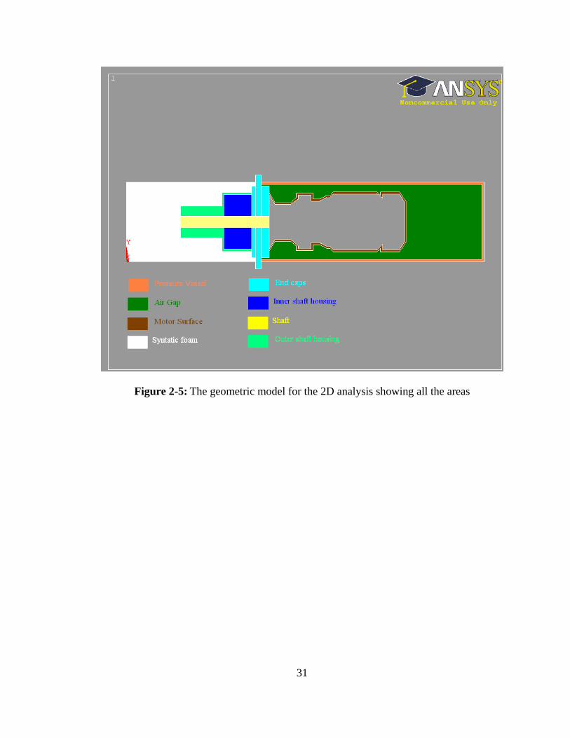
Figure 2-5: The geometric model for the 2D analysis showing all the areas
31

2.10 Meshing
Figure 2-6: Meshing of the design domain
2.11 Axisymmetric analysis
For the simplification of the design domain we have considered the geometry as an
axisymmetric problem, that is, a problem in which the geometry, loadings, boundary
conditions and materials are symmetric with respect to an axis is one that can be solved
as an axisymmetric problem instead of as a three dimensional problem. The axis of
symmetry is taken as the global y-axis.
The axisymmetric model created using ANSYS modeling is shown in the Figure 2-7.
32

Figure 2-7: Axisymmetric ANSYS model
33

2.12 Initial and boundary conditions
Boundary conditions:
Two types of boundary conditions are considered here:
1) Temperature on the outer surface of the pressure vessel ( C0 )
2) Heat flux boundary condition on the motor surface ( 2/ mW )
Initial Condition:
The initial condition is taken as the ambient ocean water temperature.
2.13 ANSYS Results
The final temperature distribution of the axisymmetric domain in 2D and 3D cases after
applying initial and boundary conditions are shown in the Figures 2-8 and in 2-9.
2.14 Fin Solution
The fin will act as heat sink. The fin (it’s a ring fin) solution technique is heuristic
solution technique, that is, it involves trial and error method. Since we have information
about the final temperature distribution inside the pressure vessel and we want to keep it
below 70 (343 ), the heuristic design procedure is chosen. 0C 0 K
Run -1: Since, form the 2D simulation the back side of the motor appears to be the
hottest, first we put a single fin (with the calculated dimensions) on the back side of the
motor and run the simulation. The maximum temperature is now reduced to 399.52 0 ,
which is still a lot higher than our safe target temperature 323 .
K
0 K
Run – 2: The single fin is splitted into two equal parts and one is put on back side and
temperature is reduced to 359 0 . one on around the gear box. The K
34

And so on.
After several these types of runs and splitting the fins and moving back and forth we
finally came up with the following temperature distribution with five tin fins:
Figure 2-8: Temperature distribution (2D) after 24 hours (in K0 ) without any fin
35

Figure 2-9: Final temperature distribution (3D) after 24 hours (temp are in K0 )
It is seen that the final temperature distribution is pretty close to the target temperature
after using five fins.
36

Figure 2-10 : Final temperature distribution with five tin fins (temps are in K)
2.15 Chapter Summary
37
In this chapter a finite element modeling of the heat transfer in the ocean current turbine
is described. Finite element analysis is an approximate numerical method. The numerical
simulation of heat transfer problems is now a standard part of engineering practice.
Before applying this numerical approximate solution, experimental and analytical
validation must be carried out. But the analytical solution, which can be used to validate
the finite element method and other numerical methods, is rather limited in the literature,
especially for the problem considered here.

38
In fact, everything depends on the problem to solve. We took into consideration all the
symmetries presented by the problem for which the corresponding boundary conditions
are written clearly from a mathematical point of view. We made use of revolution
symmetry, which is the most productive one as it allows us to carry out 3D analysis on a
plane model representing a meridian section of the studied structure. In the case of
axisymmetric analysis, a 2D model is sufficient (in the case of repetitive structure in one
direction for example). Analysis of 2D model is preferable as the analysis and
interpretation of results are always easier than a 3D model.
At the last point it can be said that among the various numerical techniques available
today, the finite element method is the most widespread owing to:
• its general fields of application (thermal, electromagnetics, structural mechanics,
fluid mechanics, etc.),
• its capacity to treat problems with complex geometries,
its easy implementation due to automation.

39
CHAPTER 3 NEURAL NETWORK ANALYSIS of HEAT TRANSFER
3.1 Introduction
The problem of complex geometry and associated boundary conditions for calculating
heat transfer can be alleviated by using artificial neural networks (ANNs). ANNs have
been developed in recent years and used successfully in many application areas, thermal
engineering (Sen and Yang, 1999) is one of them. Some examples are heat transfer data
analysis (Thibault and Grandjean, 1991), manufacturing and materials processing
(Mahajan and Wang, 1993; Marwah et al., 1996), solar receivers (Fowler et al., 1997),
convective heat transfer coefficients (Jambunathan, et al., 1996), and HVAC control
(Jeannette et al., 1998). Section 1.2.1 describes the application of ANN in thermal
engineering. The most attractive advantage of the method is that it allows the modeling of
complex systems without requiring detail knowledge of the physical processes. Because
of this, and it’s inherent characteristics for handling incomplete information, generalizing
the acquired knowledge, and tolerance for imprecision, ANNs may provide attractive
options to capture the intrinsic patterns that govern the behavior of heat transfer in
complex domain.
Thus, the current chapter concentrates on using ANNs for the approximation of the
performance of heat transfer inside the pressure vessel when different numbers

40
of fins are used. As has been the case throughout this document, ANSYS data related to
this problem, will be used here. First, some generalities about the ANN will be given.
Later the focus will be on the issue of separation of data for training and testing the
neural network. Finally, the maximum temperature generated inside the pressure vessel
using different numbers of fins will be computed using this soft computing approach.
3.2 Artificial Neural Network:
An Artificial Neural Network (ANN) is an information processing paradigm that is
inspired by the way biological nervous systems, such as the brain, process information. A
great deal of literature is available explaining the basic construction and similarities to the
biological neurons. The discussion here is limited to a basic introduction of several
components involved in the ANN implementation.
Neural networks are composed of simple elements operating in parallel. These elements
are inspired by biological nervous systems. As in nature, the connections between
elements largely determine the network function. A neural network can be trained to
perform a particular function by adjusting the values of the connections (weights)
between elements.
Typically, neural networks are adjusted, or trained, so that a particular input leads to a
specific target output. The next figure illustrates such a situation. There, the network is
adjusted, based on a comparison of the output and the target, until the network output
matches the target. Typically, many such input/target pairs are needed to train a network.

Neural Network including connections (called weights) between neurons
Compare Input
Target
Adjust weights
Figure 3-1: Typical Neural Network
Neural networks have been trained to perform complex functions in various fields,
including pattern recognition, function approximation, identification, classification,
speech, vision, and control systems. Neural networks can also be trained to solve
problems that are difficult for conventional computers or human beings.
3.2.1 Neuron Model:
3.2.1.1 Simple Neuron:
A single-input neuron is shown in Figure 3-2. A neuron with a single scalar input and no
bias appears on the left.
41

f ∑an w p f w
pn
b
Inputs General Neuron General Neuron Inputs
)(wpfa = +b
1
)(wpfa =
a
Figure 3-2: Single-Input Neuron
The scalar input p is transmitted through a connection that multiplies its strength by the
scalar weight w to form the product wp, again a scalar. Here the weighted input wp is the
only argument of the transfer function f, which produces the scalar output a. The neuron
on the right has a scalar bias, b. The bias can be viewed as simply being added to the
product wp as shown by the summing junction or as shifting the function f to the left by
an amount b. The bias is much like a weight, except that it has a constant input 1.
The neuron output is calculated as
)( bwpfa += ……………………………………. (3.1)
42
The transfer function net input n, again a scalar, is the sum of the weighted input wp and
the bias b. The sum is the argument of the transfer function f. Here f is a transfer function,
typically a step function or a sigmoid function, that takes the argument n and produces
the output a. Note that w and b are both adjustable scalar parameters of the neuron. The
central idea of neural network is that such parameters can be adjusted so that the network
exhibits some desired or interesting behavior. Thus, a network can be trained to do a
particular job by adjusting the weight or bias parameters, or perhaps the network itself
will adjust these parameters to achieve some desired end.

3.2.1.2 Neuron with Vector Input:
Typically, a neuron has more than one input. A neuron with R-input is shown in Figure 3-
3. Here the individual element inputs
Rppp ,......., 21 ………………………………. (3.2)
43
Figure 3-3: Simple neuron with vector input
are multiplied by weights
Rwww ,12,11,1 ,......., ………………………………… (3.3)
and the weighted values are fed to the summing junction. Their sum is simply , the
dot product of the (single row) matrix and the vector .
Wp
W p
The neuron has a bias b, which is summed with the weighted inputs to form the net input
n. This sum, n, is the argument of the transfer function f.
bpwpwpwn RR ++++= ,122,111,1 ....... …………….. (3.4)
The expression can be written in matrix form:
b+= Wpn …………………………………………… (3.5)
where the matrix W for the single neuron case has only one row.
∑ f aw1p
n
b1
)( bfa += Wp
Multiple-input NeuronInputs
•
•
2p
3p
Rw ,1
Rp

Now the neuron output can be written as
)( bfa += Wp ………………………………………… (3.6)
3.2.1.3 Transfer Functions:
The transfer functions in Figures 3-2 and 3-3 may be a linear or nonlinear function of n.
A particular transfer function is chosen to satisfy some specification of the problem that
the neuron is attempting to solve.
A variety of transfer functions can be found in the text books. Here the sigmoid transfer
function is used.
Log-Sigmoid Transfer Function:
The log-sigmoid transfer function is shown in Figure 3-4.
wb−
a
p
+1
-1
0
a
n0
-1
+1
44
Single-Input Log-Sigmoid Neuron Log-Sigmoid Transfer Function
Figure 3-4: Log-Sigmoid Transfer Function
This transfer function takes the input (which may have any value between plus and minus
infinity) and squashes the output into the range 0 to 1, according to the expression:
nea −+=
11 ………………………………………. (3.7)
The log-sigmoid transfer function is commonly used in multilayer networks

45
that are trained using the backpropagation algorithm.
3.3 The Network Architecture
The network architecture or topology (including: number of nodes in hidden layers,
network connections, initial weight assignments, activation functions) plays a very
important role in the performance of ANN, and usually depends on the problem at hand.
In most cases, setting the correct topology is a heuristic model selection. Whereas the
number of input and output layer nodes is generally suggested by the dimensions of the
input and the output spaces. Too many parameters lead to poor generalization (over
fitting), and too few parameters result in inadequate learning (under fitting) (Duda et al.
2001).
Every ANN consists of at least one hidden layer in addition to the input and the output
layers. The number of the hidden units governs the expressive power of the net and thus
the complexity of the decision boundary. For well-separated classes fewer units are
required and for highly interspersed data more units are required. The number of synaptic
weights is based on the number of hidden units representing the degrees of freedom of
the network. Hence, we should have fewer weights than the number of training points. As
a rule of thumb, the number of hidden units is chosen as n/10, where n is the number of
training points (Duda et al. 2001, Lawrence et al. 1997). But this may not always hold
true and a better tuning might be required depending on the problem.
Commonly one neuron, even with many inputs, may not be sufficient. We might need
five or ten, operating in parallel, in what we will call a “layer”. The concept of layer is
discussed below.
3.3.1 A Layer of Neurons
3.3.1.1 Single Layer
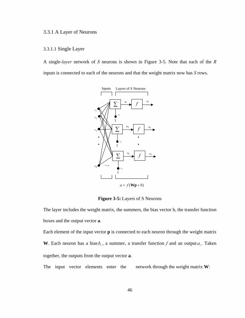
A single-layer network of S neurons is shown in Figure 3-5. Note that each of the R
inputs is connected to each of the neurons and that the weight matrix now has S rows.
46
Figure 3-5: Layers of S Neurons
The layer includes the weight matrix, the summers, the bias vector b, the transfer function
boxes and the output vector a.
Each element of the input vector p is connected to each neuron through the weight matrix
W. Each neuron has a bias , a summer, a transfer function f and an output . Taken
together, the outputs from the output vector a.
ib ia
The input vector elements enter the network through the weight matrix W:
∑ f 1aw
1p 1b
1
)( bfa += Wp
•
•
2p
3p
Rp RSw ,
∑ f
2b
1
2a
1n
2n
Inputs Layers of S Neurons
•
•
∑ f 3n Sa
Sb
1

⎥⎥⎥⎥⎥⎥⎥⎥
⎦
⎤
⎢⎢⎢⎢⎢⎢⎢⎢
⎣
⎡
⋅⋅⋅⋅⋅⋅⋅⋅⋅⋅⋅⋅⋅⋅
⋅⋅⋅⋅⋅
⋅⋅⋅⋅⋅
=
RSSS
R
R
www
wwwwww
,2,1,
,22,21,2
,12,11,1
W ……………………………….. (3.8)
3.3.1.2 Multiple Layers of Neurons
In multiple-layer networks, each layer has its own weight matrix W, its own bias vector
b, a net input vector n and an output vector a. The three hidden-layer network is shown in
Figure 3-6.
As shown, there are R inputs, neurons in the first hidden-layer, neurons in the
second hidden-layer, etc. As noted, different layers can have different numbers of
neurons.
1S 2S
The outputs of layers one and two are the inputs for layers two and three, respectively.
Thus layer 2 can be viewed as a one-layer network with inputs, neurons,
and a weight matrix . The input of layer 2 isa , and the output is .
1SR =
1
2SS =
2a21 SS × 2W
A layer whose output is the network output is called an output layer. The other layers are
called hidden layers. The network shown in Figure 3-6 has an output layer (layer 5) and
three hidden layers (layers 1 , 2 and 3).
Multilayer networks are more powerful than single-layer networks. For instance, a two-
layer network having a sigmoid first layer and a linear second layer can be trained to
approximate most functions arbitrarily well. Single-layer networks can not do
47

48
this.
At this point the number of choices to be made in specifying a network may look
overwhelming, so let us consider this topic. The problem is not as bad as it looks. First,
recall that the number of inputs to the network and the number of outputs from the
network are defined by external problem specifications. So if there are four external
variables to be used as inputs, there are four inputs to the network. Similarly, if there are
to be seven outputs from the network, there must be seven neurons in the output layer.
Finally, the desired characteristics of the output signal also help to select the transfer
function or the output layer. If an output is to be either -1 or 1, then a symmetrical
hardlimit transfer function should be used. Thus, the architecture of a single-layer
network is almost completely determined by problem specifications, including the
specific number of inputs and outputs and the particular output signal characteristic.
Now, what if we have more than two layers? Here the external problem does not tell us
directly the number of neurons required in the hidden layers. In fact, there are few
problems for which one can predict the optimal number of neurons needed in a hidden
layer. This problem is an active area of research.
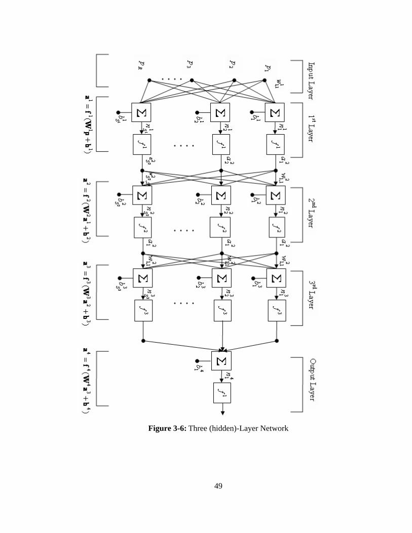
Figure 3-6: Three (hidden)-Layer Network
49

3.3.2 Learning Rules
By learning rule we mean a procedure for modifying the weights and biases of a
network. (This procedure may also be referred to as a training algorithm.) The purpose of
the learning rule is to train the network to perform some task. There are many types of
neural network learning rules. They fall into three broad categories: supervised learning,
unsupervised learning and reinforcement (or graded) learning.
In our case we used the backpropagation learning rule which is a supervised learning
rule.
3.3.2.1 Supervised Learning Training Set
In supervised learning, the learning rule is provided with a set of examples (the training
set) of proper network behavior:
{ } { } { }QQ tptptp ,,........,,,, 2211 ……………………… (3.9)
where is an input to the network and qt is the corresponding correct (target) output.
As the inputs are applied to the network, the network outputs are compared to the targets.
The learning rule is then used to adjust the weights and biases of the network in order to
move the network outputs closer to the targets.
qp
3.4 Separation of Data for Training and Testing and Network Performance
After a number of trails, the ANN structure chosen for the present analysis consists of
five layers: the input layer at the left, the output layer at the right and three hidden layers.
This 5-17-14-14-1 configuration (the next chapter describes the procedure how did we
50

come up with this architecture), where the numbers stand for the number of neurons in
each layer, is similar to the schematic shown in Figure-3-6, which is used in the
prediction of maximum temperature analysis. The inputs to the network correspond to the
numbers and the locations of fins. The output is the maximum temperature . maxT
A total of M = 942 ANSYS runs were developed for different numbers of fins and for
different positions (394 runs with 5 fins, 201 runs with 4 fins, 194 runs with 3 fins and
153 runs with 2 fins). The data can be separated in different ways into training and testing
data. For example, someone can use 60% of the total data sets available for training and
the rest for testing. This has two disadvantages: first, the data set available for training is
smaller than the total amount of information available so that the neural network model is
not the best possible, and second, if the training data do not include the extreme values
the estimation may fall in the extrapolated range and hence are less reliable. The issue of
separating the complete data into training and testing sets is further analyzed in the
following way.
The M available sets of ANSYS data are first randomly sorted to avoid introducing any
bias in the selection process and their order is then fixed. Only the first of these are
chosen for training and the rest
aM
ab MMM −= kept aside for the moment. The fraction
used for training is thus MM
P as = .
Performance Index:
The backpropagation algorithm for multilayer networks is a generalization of the least
mean square (LMS) algorithm , and both algorithms use the same performance index:
mean square error. The algorithm is provided with a set of examples of proper network
51

behavior:
{ } { } { }QQ tptptp , ..,,........., ,, 2211 ………………….…. (3.10)
where is an input to the network, and is the corresponding target output. As each
input is applied to the network, the network output is compared to the target. The
algorithm should adjust the network parameters in order to minimize the mean square
error:
qp qt
])[(][)( 22 atEeEF −==x ……………..……………. (3.11)
where is the vector of network weights and biases. If the network has multiple outputs
this generalizes to:
x
)]()[(][)( atateex −−== TT EEF …………………… (3.12)
We will approximate the mean square error by
( ) ( )∑∑==
−==
=−−=N
iii
N
ii
TT
atN
eN
kkkkkkF
1
2
1
2 11)()())()(())()(()(ˆ eeatatx
……… (3.13)
where the expectation of the squared error has been replaced by the squared error at
iteration k.
The steepest descent algorithm for the approximate mean square error is
mji
mji
mji w
Fkwkw,
,,
ˆ)()1(
∂∂
−=+ α ………………….…….. (3.14)
mi
mi
mi b
Fkbkb∂∂
−=+ˆ
)()1( α …………………….……. (3.15)
where α is the learning rate.
The mean square error (MSE) is calculated at each cycle (epoch) of the training process
in order to evaluate the performance of the network and to update the weights and biases
52

using equations (3.14) and (3.15). Here aMi ,.....,1= , where are the predictions, and
are the ANSYS values of the maximum temperatures. The stopping criterion of the
training process, however, is based on the absolute value of the mean square error. When
these error levels off, i.e., the change of rate per cycle is less than 10%, the number of
training cycles are recorded. The above is achieved with 100000 epochs, which is kept
the same for the rest of the procedure.
ka
kt
After the training is finished, three different data sets are tested: (a) the same data
that were used for training are tested, (b) the data left out of the training process are
tested, and (c) the complete M data sets are tested. In each case the percentage error
between the NN approximation and ANSYS values are calculated, being and E,
respectively. Without reordering the M datasets the procedure described above is repeated
for different values of the percentage of splitting, i.e.,
aM
bE
%,90
bM
aE ,
%,..., %9530%,20%,10=sP
and . The exact shape of the error vs. curve depends on the initial order of the data
sets, but some general features can be identified.
%99 sP
To determine the overall characteristics of the error, the curves were calculated ten times
and the results averaged to remove the influence of the initial random ordering of the data
sets. Figure 3-7 shows the average error in prediction calculated in the three different
ways as a function of the training fraction . For any , is always small since the
training and testing data are identical. At small values of , and E are both very large
indicating that an insufficient fraction of the data has been used for training. As
increases, better predictions are obtained. Beyond = 60% approximately the
SP SP
SP
SP
aE
bE
aM
53

differences in the prediction errors for all data sets are small. The same trend is observed
for the Sσ which become smaller as , indicating that the prediction is
somewhat insensitive to the initial random ordering of the data. Near the end, however, at
for example,
%100→SP
%99=SP bσ becomes large again because now is very small and the
error depends greatly on the data set that is picked for testing.
bM
The following Table 3-1 shows the results obtained with various separation of data:
% of
Data
Performance
(MSE)
Maximum Error ( )
54
C0 Standard Deviation ( ) C0
Ea bE aσ bσ σ E
10% 0.0005 1.5e-12 208.8371 208.8371 2.2e-13 51.9086 46.5103
20% 1.03 3.5364 506.9467 506.9467 0.7813 41.0977 31.8206
30% 1.61 6.6087 540.9679 540.9679 0.9629 31.6572 25.9657
40% 2.11 16.9856 178.4032 178.4032 1.6451 25.0576 20.7442
50% 2.75 12.0824 521.6405 521.6405 1.2317 20.2913 14.2845
60% 2.75 7.2591 126.4895 126.4895 1.1875 17.9252 12.2135
70% 8.00 38.2249 56.6727 56.6727 2.4632 7.9333 5.1139
80% 8.19 32.9067 33.8101 33.8101 2.2134 6.8959 4.5360
90% 8.02 20.0774 25.4156 25.4156 1.9864 5.8642 2.8711
95% 8.00 20.6020 39.2700 39.2700 1.9394 5.4446 2.4459
99% 8.00 16.4887 19.8923 19.8923 2.1184 5.2709 2.3120
Table 3-1: Standard deviation and maximum error for different % of data used

% of
Data
Performance
(MSE)
Maximum Error ( ) C0 Mean Error ( ) C0
aE bE E aμ bμ μ
10% 0.0005 1.4779e-
012 208.8371 208.8371
1.5424e-
013 28.7997 26.0787
20% 1.03 3.5364 506.9467 506.9467 0.6523 23.8047 19.3561
30% 1.61 6.6087 540.9679 540.9679 0.8302 19.8522 14.2990
40% 4.11 16.9856 178.4032 178.4032 1.1913 13.3310 8.5628
50% 2.75 12.0824 521.6405 521.6405 1.1123 14.2778 7.7789
60% 2.75 7.2591 126.4895 126.4895 1.1602 9.7679 4.6600
70% 10.52 38.2249 56.6727 56.6727 2.1132 5.7084 3.2123
80% 8.02 32.9067 33.8101 33.8101 1.7706 4.7440 2.3861
90% 8.19 20.0774 25.4156 25.4156 2.0616 4.6575 2.4319
95% 8.00 20.6020 39.2700 39.2700 2.0593 4.1227 2.1710
99% 9.33 16.4887 19.8923 19.8923 2.2029 4.0486 2.2614
Table 3-2: Mean error for different % of Data used Figure 3-8 shows the comparison of the mean error and standard deviation vs. % of data
used.
The results for various are compared and are shown in the Figures 3-9 to 3-17. SP
55

Figure 3-7: ANN prediction error vs. percentage of data used
Figure 3-8: Standard Deviation Vs. % of data used
56

Figure 3-9: Testing of the NN with same set of training data from 10% to 40%
Figure 3-10: Testing of the NN with the leftout data ranging from 10% to 40%
57

Figure 3-11: Testing of the NN (trained with 10% - 40% data) with the total data
Figure 3-12: Testing of the NN with same set of training data from 40% to 70%
58
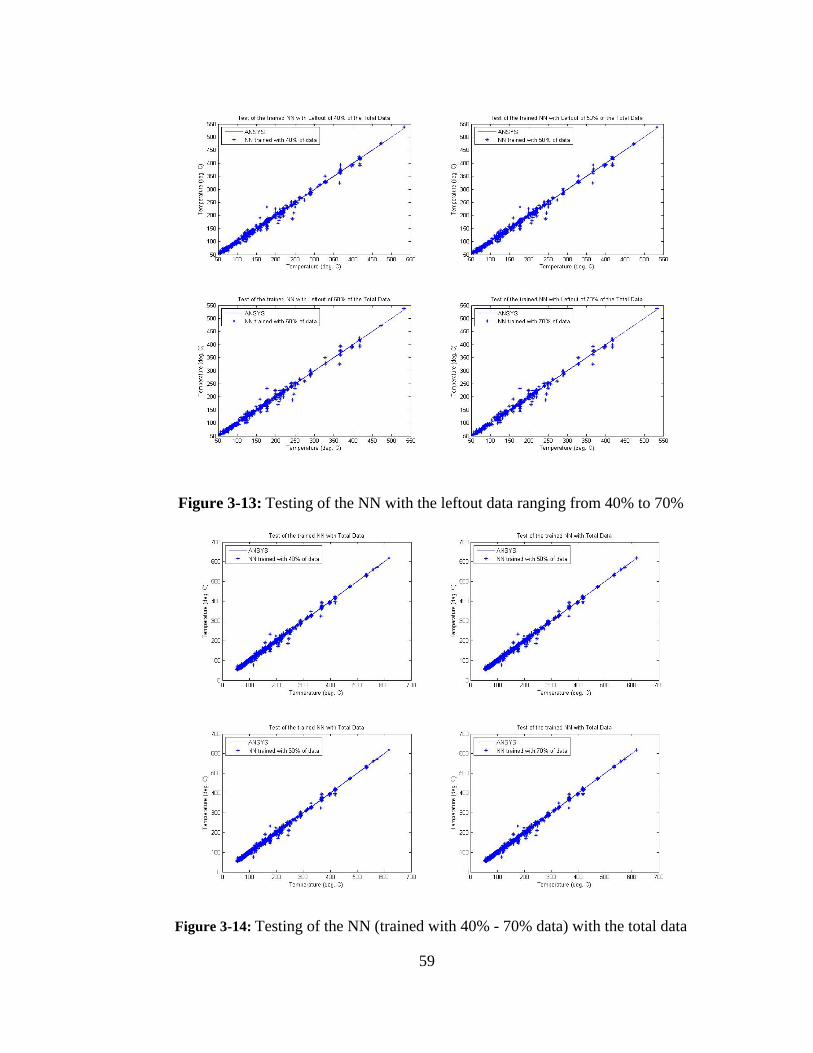
Figure 3-13: Testing of the NN with the leftout data ranging from 40% to 70%
Figure 3-14: Testing of the NN (trained with 40% - 70% data) with the total data
59
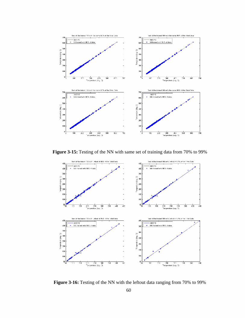
Figure 3-15: Testing of the NN with same set of training data from 70% to 99%
Figure 3-16: Testing of the NN with the leftout data ranging from 70% to 99%
60

Figure 3-17: Testing of the NN (trained with 80% - 99% data) with the total data
3.5 Postprocessing the Data
The performance of a trained network can be measured to some extent by the errors on
the training, validation, and test sets, but it is often useful to investigate the network
response in more detail. One option is to perform a regression analysis between the
network response and the corresponding targets. The MATLAB routine postreg will
perform this analysis.
If we use the MATLAB postreg routine, the network output and the corresponding
targets are passed to postreg. It returns three parameters. The first two, m and b,
correspond to the slope and the y-intercept of the best linear regression relating targets to
61

network outputs. If there were a perfect fit (outputs exactly equal to targets), the slope
would be one, and the y-intercept would be 0. For example, the post regression analysis is
performed for the trained neural network with 99% of total data and is shown in the
Figure 3-18. In this example, we can see that the numbers are very close. The third
variable returned by the routine is the correlation coefficient (R-value) between the
outputs and targets. It is a measure of how well the variation in the output is explained by
the targets. If this number is equal to 1, then there is perfect correlation between targets
and outputs. In the example, the number is very close to 1, which indicates a good fit.
3.6 Improving Generalization (Validation stop)
One of the problems that occur during neural network training is called overfitting. The
error on the training set is driven to a very small value, but when new data is presented to
the network the error is large. The network has memorized the training examples, but it
has not learned to generalize to new situations.
One method for improving network generalization is to use a network that is just large
enough to provide an adequate fit. The larger network we use, the more complex the
functions the network can create. If we use a small enough network, it will not have
enough power to overfit the data.
Unfortunately, it is difficult to know beforehand how large a network should be for a
specific application. One of the methods for improving generalization is early stopping.
Early Stopping:
In this technique the available data is divided into three subsets. The first subset is the
training set, which is used for computing the gradient and updating the network weights
62

and biases. The second subset is the validation set. The error on the validation set is
monitored during the training process. The validation error normally decreases during the
initial phase of training, as does the training set error. However, when the network begins
to overfit the data, the error on the validation set typically begins to rise. When the
validation error increases for a specified number of iterations, the training is stopped, and
the weights and the biases at the minimum of the validation error are returned.
Figure 3-18: Post regression of the trained Neural Network
63

The test set error is not used during training, but it is used to compare different models. It
is also useful to plot the test set error during the training process. If the error in the test set
reaches a minimum at a significantly different iteration number than the validation set
error, this might indicate a poor division of the data set. Figure 3-19 shows a sample
training session.
Figure 3-19: Typical training session of a Neural Network
64
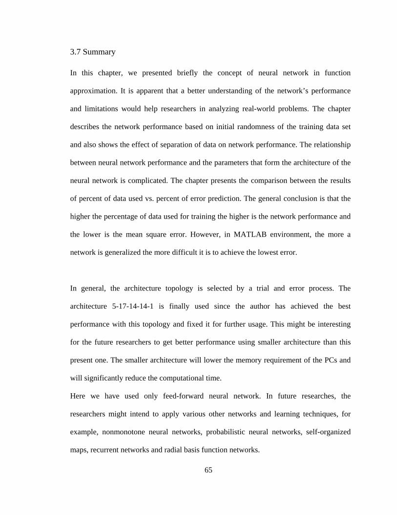
3.7 Summary
In this chapter, we presented briefly the concept of neural network in function
approximation. It is apparent that a better understanding of the network’s performance
and limitations would help researchers in analyzing real-world problems. The chapter
describes the network performance based on initial randomness of the training data set
and also shows the effect of separation of data on network performance. The relationship
between neural network performance and the parameters that form the architecture of the
neural network is complicated. The chapter presents the comparison between the results
of percent of data used vs. percent of error prediction. The general conclusion is that the
higher the percentage of data used for training the higher is the network performance and
the lower is the mean square error. However, in MATLAB environment, the more a
network is generalized the more difficult it is to achieve the lowest error.
In general, the architecture topology is selected by a trial and error process. The
architecture 5-17-14-14-1 is finally used since the author has achieved the best
performance with this topology and fixed it for further usage. This might be interesting
for the future researchers to get better performance using smaller architecture than this
present one. The smaller architecture will lower the memory requirement of the PCs and
will significantly reduce the computational time.
Here we have used only feed-forward neural network. In future researches, the
researchers might intend to apply various other networks and learning techniques, for
example, nonmonotone neural networks, probabilistic neural networks, self-organized
maps, recurrent networks and radial basis function networks.
65

66
As it is seen that the performance of an artificial neural network very much depends on
its generalization capability, which in turn is dependent upon the data representation. One
important characteristic of data representation is uncorrelated. In other words, a set of
data presented to an artificial neural network should not consist of correlation
information.

CHAPTER 4
THE NETWORK ARCHITECTURE and PERFORMANCE
4.1 Maximum temperature Analysis using Neural Network
4.1.1 Network architecture
The analysis of maximum temperature considers the fully connected feedforward neural
network. The architecture of this ANN, schematically illustrated in Figure 4-5, has one
input layer, three hidden layers and one output layer. Also, the sigmoid activation
function for the neurons in the hidden and output layers is used and the weights are
adjusted by the backpropagation algorithm.
Choice of Network Architecture:
Multilayer networks can be used to approximate almost any function, if we have enough
neurons in the hidden layers. However, we cannot say, in general, how many layers and
how many neurons are necessary for adequate performance. A network with only two
layers (input and output) can only represent the input with whatever representation
already exists in the input data. Hence, if the data are discontinuous or nonlinearly
separable, the innate representation is inconsistent, and the mapping can not be learned.
Adding a third (middle) layer to the artificial neural network allows it to develop its own
internal representation of this mapping. Having this rich and complex internal
67

representation capability allows the hierarchical network to learn any mapping not just
linearly separable ones.
Some guidance to the number of neurons in the hidden layer is given by Kolmogorov’s
theorem as it is applied to artificial neural networks. In any artificial neural network, the
goal is to map any real vector of dimension m into any other real vector of dimension n.
let us assume that the input vectors are scaled to lie in the region from 0 to 1, but there
are no constraints on the output vector. Then, Kolmogorov’s theorem tells us that a three-
layer neural network exists that can perform this mapping exactly (not an approximation)
and that the input layer will have m neurons, the output layer will have n neurons, and the
middle layer will have 2m+1 neurons. Hence, Kolmogorov’s theorem guarantees that a
three-layer artificial neural network will solve all nonlinearly separable problems. what it
does not say is that
1. this network is the most efficient one for this mapping,
2. a smaller network cannot also perform this mapping, or
3. a simpler network cannot perform the mapping just as well.
Unfortunately, it does not provide enough detail to find and build a network that
efficiently performs the mapping we want. It does, however, guarantee that a method of
mapping does exist in the form of an artificial neural network (Poggio and Girosi, 1990).
For our case, we have started with an initial guess a 5-10-1 network and then used larger
and larger networks until we were able to accurately present the function.
Figures 4-1 to 4-4 show the results obtained using different architectures with different
number of neurons and different number of layers:
68

Figure 4-1: Network Responses of Architectures (a-top left corner) 5-10-1, (b-top right
corner) 5-15-1, (c-bottom left corner) 5-17-1, and (d-bottom right corner) 5-10-10-1
Figure 4-2: Network Responses of Architectures (a-top left corner) 5-15-10-1, (b-top right corner) 5-15-14-1, (c-bottom left corner) 5-15-17-1, and (d-bottom right corner) 5-17-10-1
69
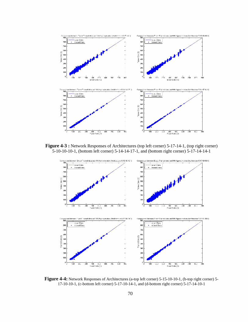
Figure 4-3 : Network Responses of Architectures (top left corner) 5-17-14-1, (top right corner)
5-10-10-10-1, (bottom left corner) 5-14-14-17-1, and (bottom right corner) 5-17-14-14-1
Figure 4-4: Network Responses of Architectures (a-top left corner) 5-15-10-10-1, (b-top right corner) 5-
17-10-10-1, (c-bottom left corner) 5-17-10-14-1, and (d-bottom right corner) 5-17-14-10-1
70

We have used the sigmoid neurons in all of the layers, that is, the transfer function for all
the neurons used is log-sigmoid. We can see some architectures in which the network
response did not give an accurate approximation to the desired function. This occurred
because the capabilities of the network were inherently limited by the number of hidden
neurons it contained. Finally, we see that the best approximation is given by the 5-17-14-
14-1 architecture. This backpropagation algorithm produced the network parameters that
minimized the mean square error. So we have saved this architecture and have used this
architecture for our optimization algorithm.
The following Table 4-1 shows the numerical comparison for different network
architectures we have tried for:
Network
Architecture MSE No of Epoch Max error (C)
Standard
Deviation (C)
5-10-1 578.41 119 250.69 34.87
5-15-1 601.53 250 260.54 33.54
5-17-1 590.65 239 259.74 30.96
5-10-10-1 580.30 279 252.36 25.66
5-15-10-1 306.32 996 133.78 11.81
5-17-10-1 170.56 487 86.38 10.16
5-15-14-1 650.63 442 275.04 26.38
5-17-14-1 156.36 1451 74.99 7.8
5-15-17-1 121.32 925 48.36 5.35
5-10-10-10-1 175.23 993 80.65 8.4
71
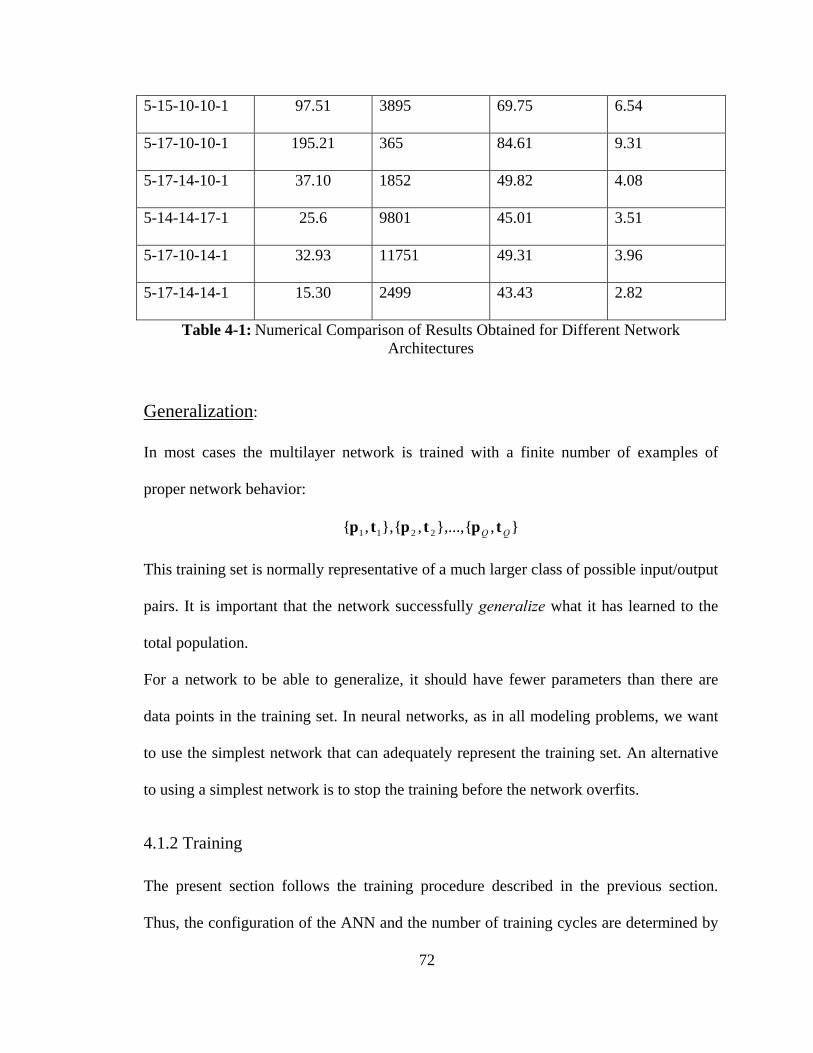
5-15-10-10-1 97.51 3895 69.75 6.54
5-17-10-10-1 195.21 365 84.61 9.31
5-17-14-10-1 37.10 1852 49.82 4.08
5-14-14-17-1 25.6 9801 45.01 3.51
5-17-10-14-1 32.93 11751 49.31 3.96
5-17-14-14-1 15.30 2499 43.43 2.82
Table 4-1: Numerical Comparison of Results Obtained for Different Network Architectures
Generalization:
In most cases the multilayer network is trained with a finite number of examples of
proper network behavior:
},{},...,,{},,{ 2211 QQ tptptp
This training set is normally representative of a much larger class of possible input/output
pairs. It is important that the network successfully generalize what it has learned to the
total population.
For a network to be able to generalize, it should have fewer parameters than there are
data points in the training set. In neural networks, as in all modeling problems, we want
to use the simplest network that can adequately represent the training set. An alternative
to using a simplest network is to stop the training before the network overfits.
4.1.2 Training
The present section follows the training procedure described in the previous section.
Thus, the configuration of the ANN and the number of training cycles are determined by
72

a trial and error process (Diaz et al, 1999) in which either may be changed if the
performance of the network during training is not good enough.
4.1.3 Network performance
The performance is evaluated by calculating the mean square error (MSE) of the output
errors
( ) ( )∑∑==
−==
=−−=M
iii
M
ii
TT
atM
eM
kkkkkkF
1
2
1
2 11)()())()(())()(()(ˆ eeatatx
………………….. (4.1)
at each stage of the training and the percentage errors between the output and target
values. Here i = 1,2,……,M, where ’s are the given training data and ’s are the
predictions, and M is the total number of training data sets. After some trials, the best
result were obtained by the 5-17-14-14-1 configuration with a number of 100,000 epochs
(training cycle).
it ia
73

1 14 17 145
Hidden Layers Output Layer Input Layer
1x
2x
3x
4x
5x
maxT
Figure 4-5: Configuration of a 5-17-14-14-1 neural network for maximum temperature prediction
4.1.4 Separation of data for training and testing
From the total of M = 942 runs that were developed in ANSYS, 394 runs =1M
74

corresponded to 5 fins, =2M 201 runs corresponded to 4 fins, 194 runs
corresponded to 3 fins and
=3M
=4M 153 runs corresponded to 2 fins.
The capability of the ANN to model complex phenomena can be illustrated by taking the
total M = 942 ANSYS runs and training a fully connected 5-17-14-14-1, shown in Figure
4-5. The N = 5 input neurons correspond to the positional of the fins variables: y; the
output neuron corresponds to the maximum temperature . The resulting function: maxT
( )wyyyyyT ;,,,, 54321maxT pmax = ……………………….. (4.2)
For testing the trained ANN, the physical variables ’s are input and the corresponding
are predicted.
iy
PTmax
4.2 Artificial neural network results
The ANN results are shown in Table 4-2 for the 5-17-14-14-1 configuration and for all
the combined fin positions and numbers. Table 4-3 shows the results obtained for
different fin positions with different architectures.
Network
Configuration MSE
Maximum Error
( ) C0
Standard deviation
( ) C0
5-17-14-14-1 15 43 2.82
Table 4-2: Network result for all fins combined
75

No. of Fins Network
Configuration MSE
Maximum
Error ( ) C0
Standard
deviation ( ) C0
5
5-17-14-14-1 1.54 33.93 2.66
5-17-14-1 3.49 188.81 9.03
5-17-1 8.72 43.11 2.35
4
5-17-14-14-1 2.31 19.65 2.82
5-17-14-1 1.03 12.65 1.90
5-17-1 8.68 23.12 3.29
3
5-17-14-14-1 1.88 34.29 4.43
5-17-14-1 1.55 48.50 5.04
5-17-1 11.44 28.76 3.59
2
5-17-14-14-1 0.01 68.85 7.96
5-17-14-1 1.54 77.84 8.58
5-17-1 21.47 42.18 5.98
Table 4-3: Network results for different no of fins with different architectures
To determine whether the network based on training data separated by some physical
condition would perform better than another trained with the combined data set, the entire
sets of runs M was combined to train a single ANN. The error, shown in Table 4-2 under
“combined”, is larger than the ANN predictions for individual cases, indicating that this
ANN has more difficulty in differentiating between the different physics involved.
However, even then the predictions of the total heat rate have errors less than 10%.
76

Figure 4-6 : Neural Network Prediction error for all-combined fins
Figure 4-7: Neural Network Prediction error for 5 fins
77

Figure 4-8: Neural Network Prediction error for 4 fins
Figure 4-9: Neural Network Prediction error for 3 fins
78

Figure 4-10: Neural Network Prediction error for 2 fins
In all the figures, the straight lines indicate quality between prediction and experiment.
The accuracy and precision given by the ANN is notable. There are some data points in
Figures 22-26 that are the outliers and can clearly be eliminated to improve the
predictions, if desired.
4.3 Error sources in ANN estimation
In order to use neural networks as a dependable tool for thermal design, one must
consider the factors that influence its predictions and performance. As mentioned by
several authors (Kramer and Leonard, 1990; Chryssolouris et al., 1996; Shao et al., 1997;
Chinnam and Ding, 1998; Niyogi and Girosi, 1999), the performance of neural networks
79
is influenced by noise corruption, spatial distribution and size of the data used to
construct the neural network model, and the characteristics of the artificial neural
network, i.e. number of layers, number of hidden neurons, its architecture, etc. The neural
network is comprised of a finite number of hidden layers and neurons per layer to
approximate an unknown function, and this fact also introduces an error. The scale of this
error depends on the figurative capability of the artificial neural network which may
increase due to over fitting as the size of the network becomes large. Another source of
error branches from the fact that only finite data are available for training. As the number
of training data sets increases, the error decreases. Niyogi and Girosi (1999)
demonstrated that it is not possible to reduce the upper bounds on errors due to the
network size and the limited training data simultaneously. Thus if we want to rely on the
ability of the neural network to generalize the connection between the input and output
quantities that govern the heat transfer phenomena inside the pressure vessel for motor-
gear box arrangement, we will have to be very careful in providing an adequate training
set. On the other hand, as a consequence of being applied to regions beyond the range of
available training data, neural networks are very likely to have a poor performance on
their predictions. In fact, for a fixed neural network architecture, we may have two limits
depending on the availability of the training data sets and the number of inputs to the
neural network. In such a case, when the number of measurements is very large, if the
network is used outside the convex hull of the training data (Courrieu, 1994), then the
error in the performance of the neural network will be large because there are no data in
the region to support the predictions. Inside the domain given by the convex hull, the
empty spaces where measurements are absent are small in size and there is little
80

degradation of the network predictions. The second limit appears when there are very few
training experiments, as in the case of the present study. The voids inside the convex hull
of the data are large enough so that they contribute to the inaccuracy of predictions made
by the neural network in these regions.
4.4 Summary
In the present study we have applied the ANN approach to accurately model the thermal
characteristics of a pressure vessel generating heat inside due to an electric motor.
Because of the inherent attributes of the ANN technique, which traditional analysis
including standard correlations do not have, ANNs can correlate given experimental data
with errors of the same order as the uncertainty of the measurements. Even when discrete
variables are involved, its ability to recognize patterns allows the neural network to
capture all the complex physics without need to assume mathematical models of the
process. These features, in principle, make the ANN approach suitable for use in the
estimation of heat rates under different conditions.
Correlations and neural networks, being empirical models of complex systems, are
constructed based on experimental information. Their effectiveness is estimating the heat
rates under operating conditions different from those used in their development, depend
on the number and distribution of these measurements. Models constructed from large,
dense and well distributed measurements will tend to have smaller errors, while those
built from undersized data will perform poorly. Limited data arise from the fact that in
industrial applications, such as underwater turbine, it is not economically possible to
perform a large number of experiments.
81

82
We have presented a methodology for the estimation of errors from an ANN trained with
a finite number of data sets. A low value of the estimated error is an indication that there
are sufficient training data to support the ANN prediction; while a large error will
indicate absence of enough points to aid in the ANN predictions and more training data
would be needed in order to improve these.
In the present case, no experiments were performed and no experimental data were
available. So, experimental validation of this design procedure is omitted. A low value of
the estimated error would be an indication that there are sufficient experimental data to
support the ANN prediction; while a large error will indicate absence of enough points to
aid in the ANN predictions and more experiments would be needed in order to improve
these. The procedure proposed here can help the design engineers and the manufacturers
to plan new measurements by showing where these are needed.

CHAPTER 5 THE DESIGN OPTIMIZATION WITH GENETIC ALGORITHM
5.1 Introduction
The design systems work by searching through the large number of possible solutions to
discover the best specific solution. The search process is often time consuming and
expensive. But by exploiting the natural processes that biological systems use to evolve
and adapt, design engineers can often quickly solve otherwise difficult design problems
that resist solution by traditional optimization methods. This chapter explains the basic
technique of the genetic algorithm and shows how we can use the genetic algorithm to
solve our particular design optimization problem.
For such problems genetic algorithms may perform better than traditional approach
because they better retain the feasible points found in their populations and may have
higher selection pressure which is desirable when evaluations are very expensive.
This chapter focuses on explaining how genetic algorithms work. Also the thermal
design optimization problem, in other words to find the best possible solutions for the fin
locations, the genetic algorithm is applied and this chapter explains the design steps.
Some more basic theoretical references are provided in the bibliography for those
interested in a more rigorous explanation of the details of genetic algorithm.
83

5.2 Basic Optimization Terminology
Here some informal definitions for a few basic optimization terms are provided in order
to ensure that everyone has a common understanding. These are not rigorous definitions,
but should be adequate for the readers. Only basic terms are presented here to get the
discussion going; other more specific terms relating to genetic algorithms are introduced
as the remainder of this chapter.
Optimization refers to a goal directed search for the “best” solution to a problem. The
idea of what is best must be defined by the problem statement. Minimizing the
temperature by searching the lowest temperature is an example of an optimization
problem. Optimization problems seek either the minimum or the maximum of some
problem specific property or set of properties, but multiple goals or objectives are not
uncommon.
The objective function is the design engineer’s numerical representation of the goal in
the optimization problem. When the objective is to minimize, the term cost function is
sometimes used. Genetic algorithms, however, use the term fitness function and that is
the term used in this chapter.
Decision variables are the independent variables in the optimization problem that the
design engineer manipulates while searching for the optimum solution. For example, the
design considered here uses the locations and width of the fins as design variables.
A constraint refers to a restriction the design engineer places on either the design
problem’s decision variables or resulting solutions. The design engineer could restrict
stress or deflections, for example.
84

A feasible solution is any solution that does not violate any of the constraints the design
engineer has placed on the problem being optimized. The feasible region consists of all
the feasible solutions taken as a whole. The more restrictive the constraints placed on the
problem by the design statement, the smaller the feasible region. Highly constrained
problems may result in an empty feasible region, which obviously has no feasible
solutions.
The search space encompasses the region that will be searched during the optimization
process. The search space includes all possible values that the decision variables can
assume. But since most problems have constraints on problem solutions, the search space
will include some solutions that are not feasible. The optimization search process will
throw out the solutions that are outside the feasible region.
5.3 Types of Optimization Problem
Optimization problem types may be categorized according to many different strategies.
The problems might be arranged in a continuum from numerically well behaved to
completely random.
• Well behaved fitness function: The fitness function of a numerically well behaved
problem is continuous and differentiable everywhere within the search space. This
fitness function can be also mono-modal having a single minimum or maximum
point that represents the optimum solution. Such a problem is easy to solve with any
of the classical methods of optimization that are referred to as hill-climbing methods.
When the fitness function is multi-modal the hill-climbing method will get stuck at
the top of the first hill encountered. To solve that problem the solution process can
85

typically start from several different locations. The best solution obtained in that
series of trails is then presumed to be the global optimum for the solution space.
• Random fitness function: At the other extreme of the problem continuum is the
objective function that appears to be completely random. This appearance of
randomness may be caused by incomplete knowledge of the parameters that control
the fitness function or the problem could truly be random. In either case the fitness
function appears to have no consistent relationship with the decision variables. The
random problem is solved by a complete exploration of the solution space. The
method is referred to as complete enumeration. The complete enumeration method,
while effective, is seldom practical.
Between these two extremes of the well behaved and the random fitness function lies the
real world problem. The real optimization problem may be discontinuous at several
points and is often discontinuous at the global optimum because of a constraint. The real
optimization problem may not be differentiable, may have many relative optimums, and
may be tightly constrained by numerous boundary conditions. But the solution is not
random; searching in the correct direction generally leads to improvements in the fitness
function. This is the type of problem that a genetic algorithm can approach and often
solve.
5.4 How Genetic Algorithms Work
The genetic algorithm is modeled roughly on how natural biological systems evolve and
adapt through the process of natural selection. Many analogs with biological systems are
used to explain the operation of the genetic algorithm. The genetic algorithm approach
86

differs form that of the more traditional hill-climbing and complete enumeration methods
in four basic ways.
First, the classic genetic algorithm encodes the values of the decision variables in a string
called a chromosome. The encoding and the interpretation of the string are devised by the
design engineer, but the computer interprets the string as simply a string of binary digits.
Each bit can be thought of as a gene in the chromosome.
Second, the genetic algorithm uses a population of individuals to perform the search.
Each individual represents one possible solution to the problem. The individual’s
chromosome encodes one set of decision variables and so results in a single point in the
solution space.
Third, evaluation of search progress is based on fitness alone, which keeps the search
focused on the actual objective the design engineer is seeking. Derivatives are not used so
the expense of derivative calculation is not incurred. Since derivatives are not used the
method is not affected by discontinuous functions.
Fourth, the genetic algorithm is not a random search method, but it does use random
processes to transition from one search state to another. The random processes give
genetic algorithms a good balance between wide exploration of the search space and
exploitation of fitness landscape features. Recall that enumeration techniques are very
good at exploration, but do not exploit local features. Hill-climbing methods, however,
are very good at exploitation, but do not explore the entire search space.
The genetic algorithm uses the selection, recombination, and mutation operations on the
population of individuals to perform the search. The population is randomly created at the
start of the search. Fitness is used to select individuals from the current generation to
87

advance into the next generation. These individuals are recombined and possibly mutated
to form the next generation. This process is continued until there is no change in the best
individual in the population.
Selection begins by determining the relative fitness of each individual by calculating the
individual’s fitness divided by the total fitness of the entire population. Then a
cumulative fitness is calculated for each individual as the sum of the relative fitness for
all members up to the one being calculated. The cumulative fitness is thereby normalized
over the entire population to a maximum of 1.0 for the last individual.
The population can be thought of as forming a roulette wheel with slots proportional to
that individual’s fitness relative to the rest of the population. A random number between
0 and 1.0 is generated next and the individual with the cumulative fitness that bounds the
random value is selected. This selection process continues until a new population is
formed. In general, those individuals with higher fitness values are more likely to be
selected, but there is an element of random choice also. Similarly, multiple individuals
that have the same chromosome and hence the same fitness will also have a better chance
of being selected.
Once the new population of individuals is selected recombination begins. The genetic
algorithm moves through the population by pairs and randomly determines if each
individual pair will be recombined. If that is the case, a random point along the pair of
chromosomes is selected and the remainder of each chromosome to the right of the
selection point is swapped between the two chromosomes. Two new individuals are
formed, which are a recombination of the genes in the original two chromosomes.
Finally, each gene of each chromosome of each individual may be randomly mutated in
88

order to introduce additional diversity in the population. The probability of a mutation is
generally low, but the design engineer can control this and all other probabilities to fine
tune the search process.
Since most real world problems have constraints, the genetic algorithm needs a
mechanism for applying problem constraints. A penalty function is an easy way to
constrain the behavior of the fitness function to the feasible region by applying a penalty
for violating a problem constraint. A penalty function reduces the value of the fitness
function when a constraint is violated. A good penalty function drops the value of the
fitness sharply at the constraint boundary forming a cliff in the fitness landscape. Recall
that discontinuities do not bother the genetic algorithm so the sharper the edge of the cliff
the better.
Good results can be obtained by reducing the unconstrained fitness value with a penalty
that increases exponentially as the constraint violation increases. The violation squared
can be subtracted from the value of the fitness function or the fitness can be multiplied
by:
|violation|−e .
Since the genetic algorithm uses random process to transition from one generation to the
next, the genetic algorithm is not deterministic. That is to say it is unlikely the same
answer will be obtained in any two attempts with the same problem. The answer will be
the best that the genetic algorithm can find. The genetic algorithm does explore broadly,
however, and exploits the fitness landscape to find a very good solution.
89

90
5.5 The Numerical Design Optimization Problem
In a very general form, the engineering numerical design optimization problem can be
stated as follows: given a computer tool that can evaluate a design, the goal is to use this
tool to come up with the best design according to some measure of merit and subject to
some constraints, on condition that this is done within the time limits. The tool is usually
a simulator or a piece of analysis code. The measure of merit may be a function of
manufacturing cost, quality, stability or any combination of these and/or similar
properties. The “thing” to be designed may be a machine or a process. The constraints
may be performance related or modeling related.
For example, the problem may be to design a pressure vessel inside which a heat source
is active and the inside temperature is to remain always below a certain degree of Celsius.
The design may consider using fins to keep the temperature below the threshold
temperature. The goal may be to minimize the number of fins, minimize the total mass
weight of the fins and to find the best locations for the fins. The constraints may include
something like “the fins must be in the positions on the motor-gear box where it is
feasible to install in,” or “the widths of the fins must be sufficient and strong enough to
withstand under severe vibration condition,” or “the total mass weight of the fins must be
limited to certain kilograms so that the pressure vessel is structurally stable”. The time
limits for the design optimization may be a few hours (as in a quick feasibility study) or a
few months (in the case of final product design).
In the most general form, the word “design” may be taken to mean any kind of decision
making regarding the shape or composition of some artifact. More formally, it could
mean structural design or parametric design or both. Structural design involves

making decisions about the overall shape of the system (for example, how many fins the
thermal design for the pressure vessel should have). Most variables involved in structural
design are discrete. Parametric design involves making more detailed decisions about
numerical aspects of the design (for example, what the length and width of the fins
should be). Most variables involved in parametric design are continuous.
Once we make these assumptions, the problem becomes a general constrained non-linear
programming problem in which the objective function and (often) the constraints are the
outcome of the program. In other words, the problem may be stated as:
mjxxx
mjxhlixg
xf
UL
j
i
,....,1
,....,1 0)(,....,1 0)(
osubject t)( minimize
)()( =≤≤
===≤ ………………………………… (5.1)
where
• x is a vector of real numbers representing the parametric description of the object
being designed. The vectors )(Lx and )(Ux represent the lower and upper bounds
of the design parameters respectively.
• )(xf is the objective function. It represents a numerical property of the object
being designed, which needs to be minimized (such as temperature).
• )(xgi and )(xhj are the inequality constraints and the equality constraints
respectively.1 These constraints are a means of quality control. Some of these
constraints ensure that the design is physically realizable, others ensure adequate
1 In practice, equality constraints are usually converted to inequalities by introducing a numerical threshold. For example, 0)( =xh j may be replaced by ε≤)(xh j where ε is a small constant.
91

• performance and the rest ensure that the design is within the limits of the model
being used.
Constraints are usually handled in one of two ways:
• Direct methods use the gradients (usually their numerical approximations) of the
constraints to compute a direction that satisfies all constraints. Once a feasible
point is found (i.e. one that satisfies all the constraints), direct methods usually
use the gradient of the objective function and the active constraints to compute a
direction that improves the objective function while not violating any constraints.
• Penalty methods do not work directly on the constraints but instead they add a
penalty term to the objective function to account for constraint violations if any
and then unconstrained optimization is performed using the augmented objective
function. The penalty term is usually the product of a (large) positive penalty
coefficient times the sum of the constraint violations.
The problem of proving that a point is a local optimum of a general nonlinear
programming problem is undecidable (Schwabacher 1996). Therefore there is no
analytical solution to the above problem. On the otherhand there is a large amount of
literature on how to solve the nonlinear programming problem in practice. Most such
techniques do not take into consideration the special properties of engineering design
optimization spaces.
5.6 Thermal Design Optimization with genetic algorithm
Though GAs are relatively new technique in relation to its application to thermal
engineering, there are a number of different applications that have already abeen
92

successful. The GA application in thermal engineering has been discussed in the Section-
1.2.2.
5.6.1 Genetic Algorithm (GA) Architecture
This section provides a detailed description of the genetic algorithm specifically designed
and tailored to be used for thermal design optimization for the problem stated in Chapter
1. The GA is designed from the existing techniques from the literature.
5.6.1.1 Overview of the Genetic Algorithm
The genetic algorithm is detailed described and mentioned in the references (Goldberg,
1989). In the remainder of this section we describe the main components of a genetic
algorithm that has been used for our design process in the context of numerical
optimization.
5.6.1.1.1 Representation (genotype)
In order to use genetic algorithms it is necessary to map the solutions of the problem to
fixed length strings of some alphabet. The resulting strings are called the representation
(genotype in GA terminology). The most common representations are binary and
floating point.
Each individual of this tailored GA population represents a parametric description of the
artifact, such as the locations and widths of fins. All parameters have continuous
intervals. Here we used floating point representation (genotype). The fitness of each
individual is based on the sum of a proper measure of merit computed by a simulator or
some analysis code (such as the weight of fins), and a penalty function if relevant (such
93

as to impose limits on the permissible size of a fin). The penalty function is the product of
an adaptive penalty coefficient and the sum of the constraint violations if any.
5.6.1.1.2 Initialization
In order to start the genetic algorithm evolution process, an initial population of solution
vectors must be generated. The most common method of initialization is GAs is random
initialization in which the initial population consists of random vectors uniformly
distributed in the search space hypercube.
Here the initial population is generated randomly in between 0 and 1.37m, since we want
to put the fins on the top of the motor surface.
5.6.1.1.3 The Selections Strategy
The selection strategy decides how to select individuals to be parents for newborns.
Usually the selection applies some selection pressure by favoring the individuals with
better fitness. The most common selection methods are:
• Fitness proportional (roulette wheel) selection: each individual’s probability
of being selected is proportional to its fitness value.
• Rank-based selection: each individual’s probability of being selected depends
on its fitness rank in the population rather than the actual fitness value. The
most common rank-based selection methods are:
o Tournament selection
o Weight series selection
94

We use fitness proportional selection methods. Each individual x is selected and copied
in the mating pool with the probability proportional to fitness, ∑
=)(
)(xf
xfps . This is
implemented using a roulette wheel method.
5.6.1.1.4 Genetic Operation
Crossover Operation
Single-point crossover is assumed. In this operation two parent individuals are selected
from the mating pool.
The point crossover operator aligns the genotypes of the parents. A crossover position
is then randomly selected with uniform probability and the part of the first parent’s
genotype before the crossover position is copied to the corresponding part of the
newborn. The rest of the newborn comes from its corresponding place in the second
parent’s genotype.
Crossover operation is executed with the probability . cp
95
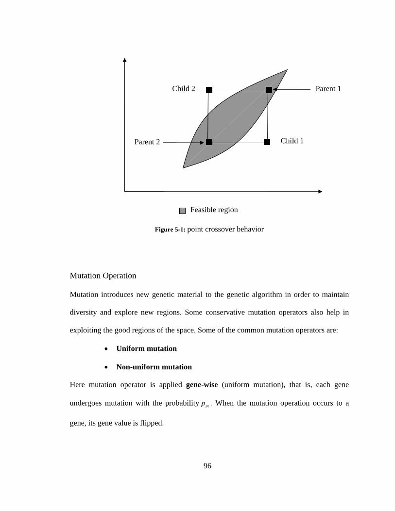
Child 1 Parent 2
Child 2 Parent 1
Feasible region
Figure 5-1: point crossover behavior
Mutation Operation
Mutation introduces new genetic material to the genetic algorithm in order to maintain
diversity and explore new regions. Some conservative mutation operators also help in
exploiting the good regions of the space. Some of the common mutation operators are:
• Uniform mutation
• Non-uniform mutation
Here mutation operator is applied gene-wise (uniform mutation), that is, each gene
undergoes mutation with the probability . When the mutation operation occurs to a
gene, its gene value is flipped.
mp
96

5.6.1.1.5 Replacement strategy
The replacement strategy is unique to steady state genetic algorithms. It decides how to
make room for the newborn when the population is full. Some of the most common
replacement strategies are:
• Elitist replacement: selects for replacement a random individual, on
condition that the best elite fraction of the population is not replaced. The
elitist fraction may be constant or dynamic.
• Crowding replacement: takes into consideration others factor in addition
to fitness (such as preserving diversity in the population for example).
The reader is referred to [Mahfoud 1995] for a detailed description of this
method.
5.6.1.1.6. Stopping criteria
The genetic algorithm stops when either the maximum number of evaluations has been
exhausted or the population losses diversity and practically converges to a single point in
the search space.
5.7 Thermal Design Application domain: Motor-gear box arrangement domain
inside pressure vessel of an ocean turbine
5.7.1 Domain description
Our domain concerns the already built motor-gearbox arrangement which is installed
97

inside a pressure vessel of an ocean turbine. Figure 5-2 shows the simplified schematic of
the arrangement which is created in ANSYS for the finite element analysis of heat
transfer.
Lets say the position of five fins are . 54321 and ,,, yyyyy
The fitness function for the genetic algorithm is designed as:
bwyfwyfwyfwyfwyfwTwJ w++++++= )()()()()(min 5544332211max0 … (5.2)
where
w = weights assigned
= function of the positions of fins )(yf
The weights will be assigned depending on the positions of the fins. The design domain is
divided depending on the most and least favorable positions of the fins.
Figure 5-2: Simplified schematic arrangement of the ocean turbine
98

Figure 5-3: The design domain
5.7.2 Dividing the domain
Figure 5-3 shows the division of the domain of interest, that is, the motor-gear box
surface.
Most favorable positions:
121
LyL mi ≤≤
342
LyL mi ≤≤
783
LyL mi ≤≤
10114
LyL mi ≤≤
99
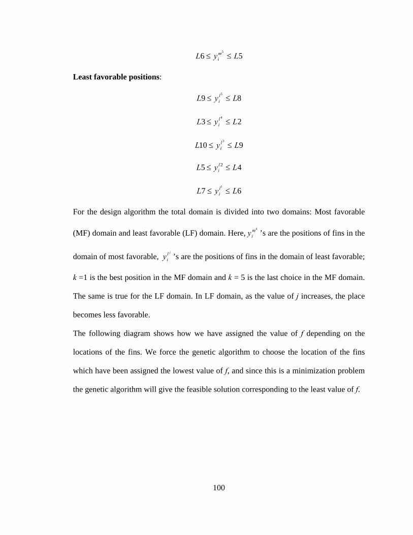
565
LyL mi ≤≤
Least favorable positions:
895
LyL li ≤≤
234
LyL li ≤≤
9103
LyL li ≤≤
45 2 LyL li ≤≤
671
LyL li ≤≤
For the design algorithm the total domain is divided into two domains: Most favorable
(MF) domain and least favorable (LF) domain. Here, ’s are the positions of fins in the
domain of most favorable, ’s are the positions of fins in the domain of least favorable;
k =1 is the best position in the MF domain and k = 5 is the last choice in the MF domain.
The same is true for the LF domain. In LF domain, as the value of j increases, the place
becomes less favorable.
kmiy
jliy
The following diagram shows how we have assigned the value of f depending on the
locations of the fins. We force the genetic algorithm to choose the location of the fins
which have been assigned the lowest value of f, and since this is a minimization problem
the genetic algorithm will give the feasible solution corresponding to the least value of f.
100

565
LyL mi ≤≤
10114
LyL mi ≤≤
783
LyL mi ≤≤
342
LyL mi ≤≤
121
LyL mi ≤≤
671
LyL li ≤≤
452
LyL li ≤≤
9103
LyL li ≤≤
234
LyL li ≤≤
Lower the value of f
895
LyL li ≤≤
Figure 5-4: The geometric division of the design domain
101

5.8 Genetic Algorithm Flowchart
Starting generation G = 0
Initialization of random population
Termination criterion satisfied?
or maxGG ≥
Select M individual based on fitness
Designate result
End
j = 1
?Mj ≤
Evaluation of fitness of each individual in population
Evaluation of fitness of each individual in population
Yes
No
j = 1 No
Select two individual
Perform crossover with probability cp
Insert two offspring into new population
j = j+2
Yes
?Mj ≤
Select one individual
Perform mutation with probability mp
Insert individual into new population
j = j+1
G =G+1
j = a member in the population G = number of current generation
No
Evaluation of fitness of each individual in
population
Yes
Figure 5-5: Flow chart for the genetic algorithm
102

5.9 Optimum Results Obtained with Genetic Algorithm:
One of the advantages of GA is that it provides a list of optimum variables, not a single
solution. Also the optimum solution is independent of initial population generation. We
have generated the pool of individuals (the initial population) in two different ways, first
restricting the random population in the range of 0 to 1.37 m and secondly, generating
random numbers without any restrictions, or initial range.
Population 1: pop =0.0001+(1.37-0.0001*rand (Npop, Nvar))
Population 2: pop = rand (Npop, Nvar)
A population of 500 individuals was used. The probability of recombination was 0.8 and
the probability of mutation was 0.03. It should be remembered that the GA uses a random
number generator, so the exact result won’t be reproducible.
Table 5-1 shows the optimum results obtained from GA and comparison with ANSYS:
103

Comparison between Genetic Algorithm and ANN:
GA results ( ) CT 070max ≤Temperature ( ) C0
Positions of Fins
Initial population
range
1y 2y 3y 4y 5y GA
NN
(5-17-14-14-1)
37.10 ≤≤ pop
0.887 0.807 0.514 0.914 1.274 56. 3 56.21 0.524 0.789 0.878 0.911 1.264 69.2 69.15 0.847 0.922 1.150 0.658 0.558 69.2 69.24 0.538 0.976 1.139 1.347 0.871 69.4 69.43 1.173 1.292 0.689 0.948 0.513 68.9 68.96 1.036 0.699 0.495 1.102 0.610 69.2 69.30 1.157 1.145 0.554 0.804 0.680 67.8 67.88 1.130 1.164 0.593 0.848 0.558 65.1 65.16 1.177 0.636 0.498 0.920 0.840 57.2 57.23 0.587 0.499 0.852 0.925 1.177 60.2 60.20 0.966 1.323 0.717 0.517 1.292 67.5 67.56 0.596 1.129 0.718 0.555 1.098 62.2 62.27 0.637 1.092 0.732 1.174 0.553 64.1 64.08 0.958 0.537 1.205 1.040 0.651 70.5 70.50
rand (Npop, Nvar)
0.900 0.905 0.814 0.917 0.516 59.9 59.89 0.518 0.860 0.993 0.954 0.532 59.6 59.65 0.521 0.984 0.910 0.879 0.546 62.6 62.58 0.522 0.918 0.915 0.554 66.9 66.91 0.894 0.815 0.858 0.923 0.516 68.8 68.73 0.947 0.599 0.894 0.947 0.500 68.8 68.76 0.970 0.513 0.846 0.859 0.840 69.9 69.99 0.828 0.924 0.921 0.517 0.836 69.8 69.88
Table 5-1: Comparison of GA results with ANSYS results
Table 5-1 shows despite of the method of initial population generation, the GA gives
almost the same optimum temperatures. The entire above solutions lie in the feasible
region satisfying all of the imposed constraints and also the results agree with the
corresponding ANSYS results. These solutions give the pareto-optimal set. These are the
104

set of design variables given by the GA, since in GA the initial population is generated
randomly; the final results vary each time GA is run. So, if one of these five locations is
chosen for the fin installments, it is guaranteed that the temperature inside the pressure
vessel will be below the specified minimum temperature.
5.10 Chapter Summary
This chapter describes a design algorithm for finding the optimum number and locations
for fins. We have discussed the modeling and architectural aspects of our design
optimization. The advantage of this method is that it does not need a rigorous
mathematical objective function for its function evaluation. The genetic algorithm uses
the neural network approximation, described in previous chapters, as it’s objective
function. However, the design algorithm and the genetic algorithm used here have been
made as simple as it could be. We have put only the locations and numbers of fins as the
design parameters. To make the design algorithm better and getting more versatile results
the following can be considered as design parameters:
a) Width of the fins
b) Cross-sectional areas of the fins
c) Mass weight
d) Material of the fins, and
e) Conductivity
Also, the constraints put here have been made as simple as it could be. For the betterment
of the optimum results the constraints cut be put in trial and error basis depending on the
geometry and decision parameters.
105

Overall, the design algorithm in its simplest form worked good and proved that it can
provide with optimum design solutions using the NN as its fitness function. The design
algorithm is carried out in MATLAB environment.
GAs are powerful optimization tools, appropriate for many applications. Some of the
challenges faced in the application of genetic algorithms to engineering design domains
are:
• The search space can be very complex with many constraints and the feasible
(physically realizable) region in the search space can be very small.
• Determining the fitness of each point may involve the use of a simulator or an
analysis code which takes a non-negligible amount of time. This simulation time
can range from a fraction of a second to several days in some cases. Therefore, it
is impossible to be inconsiderate with the number of objective evaluations in an
optimization.
For such problems genetic algorithm may perform better than conventional optimization
technique.
The genetic algorithm has some powerful advantages over both the classical hill-climbing
method and the complete enumeration method. First the genetic algorithm provides a
good balance of both exploitation and exploration of the search space. That means
solutions are efficient yet full exploration of the entire space is provided so the solver is
less likely to hang up on a local relative optimum.
Second, the genetic algorithm has no problem of a discontinuity – one of the
characteristics of many real world problems. The design engineer does not need to create
elaborate mathematical fictions, however, to fool the solver into thinking the actual
106

107
problem is well behaved.
Finally, the genetic algorithm seeks the very good solution, rather than the very best
solution. This is actually a strength that prevents the genetic algorithm from myopically
falling into holes in the mathematics or getting stuck on top of a local hot spot.

CHAPTER 6 GENERAL CONCLUSION
6.1 Summary of Benefits and Limitations for the Present Methodologies
Benefits:
If we have trained neural network and results from genetic algorithm, that is the optimum
number and locations of the fins, we can check the genetic algorithm result
instantaneously using the trained neural network. If we want to check the genetic
algorithm result with ANSYS simulation, the simulation run time is a lot higher.
Therefore it is seen that using artificial neural network, computational time lowers down
to zero.
The benefits of using the present methodology are tabulated below:
1) Fast Computation:
Computational Time (for five fins)
ANSYS ANN
56 minutes (transient
analysis)
0.2 second
2) Simplicity:
After having the optimum results from GA, the results are checked by only calling the
108

trained neural network. The trained neural network only needs the inputs, and gives the
maximum temperature as the network output. This is a very simple operation.
On the other hand, compared to ANSYS, running the ANSYS simulation is always a
complex procedure. In ANSYS, checking the genetic algorithm result with five fins
requires the following steps:
i) Modeling the fins in exact locations, defining five different areas.
ii) Defining material properties
iii) Meshing
iv) Apply Loadings and boundary conditions, and
v) Finally, solving in ANSYS
We can see that the ANSYS procedure is much more complex compared to simple ANN
implementation.
Limitations and Disadvantages:
1) Limited training data. For training the neural network, the network needs always
very large number of training pairs for better network performance. But in reality
getting large number of training sets are not possible due to physical limitations.
Also with a huge amount of training data, it takes a significant amount of time for
training the network. So, there is always a trade off between large training data
and better network performance.
Despite of very fast computation time, there are always errors involved in artificial neural
network performance, no matter how small the error is.
109

6.2 Conclusions
The present thesis has dealt with the accuracy of predictions of thermal performance of
an ocean turbine. The aim of the work presented in this thesis was to examine the
possibility of defining an optimal design algorithm for the thermal system of an ocean
turbine. To this end three types of techniques have been used. The first technique uses the
method of finite elements of heat transfer that are used to find the approximate heat
transfer solution of the considered design domain inside a pressure vessel. The second is
an adaptive function which belongs to the soft computing methodology: the artificial
neural network. And finally, the third encompasses optimization methods based on
biological evolution that are used to find the parameters of a given functional form.
The motor-gear box arrangement inside the pressure vessel of an ocean turbine is a
complex system for which the accurate determination of their performance is essential.
Due to the fact that the geometry of the arrangements and the boundary conditions are
complex, analytical solutions are not available for the heat transfer calculation; a
common practice is to use the finite element approximations for the heat transfer
calculations. The heat loss from the motor has been taken as the thermal flux boundary
conditions per square meter of the motor surface. A complete analysis has shown that
there are some percentages of error in the calculation of the transfer of heat. The current
work has also found that the reason for the lack of accuracy is because of the restrictive
simplifying assumptions have been made with respect to geometry, material properties
and boundary conditions.
In the current thesis the use of artificial neural network can be thought of as an approach
for acquiring knowledge about the heat transfer in design domain and use it to guide for
110

further explorations. We can afford to use these relatively expensive methods because the
objective functions are even more expensive. By acquiring the knowledge of heat transfer
by using neural network we can solve the problem more efficiently by optimizing each
subset separately. Artificial neural networks do not have the deficiencies of correlations;
moreover they do not need explicit mathematical representations nor detailed information
of the process. Results from the application of neural networks to the thermal design have
demonstrated that, because of its inherent attributes that allow them to recognize and
simulate nonlinear phenomena in complex processes, artificial neural networks can
correlate given data with errors of the same order as the uncertainty of measurements. In
all the cases investigated here, the estimation errors from the neural network approach are
restricted to less than 5%. Even with limited data involving discrete variables, such as
those included in motor-gear box geometry, the neural network approach is suitable to
simulate the behavior of the system.
In this project, an optimization methodology based on biological evolution that enables a
better accuracy by finding the optimum values of the design parameters is introduced. A
general purpose genetic algorithm is used for the optimization problem. Genetic
algorithms have been extensively used as a means of performing global optimization in a
simple yet reliable manner. However, in some cases of design optimization domains a
general purpose genetic algorithm is often unable to give the global optimum solution;
this may be due to the assumptions made during the different stage of the procedures.
Moreover, the constraints and the nonlinear objective functions for the genetic algorithms
can be manipulated to improve the quality of the resulting design.
The focus of this research work has been to develop methodologies that allow accurate
111

estimation of heat transfer of a given geometric domain and also that allow giving
optimum design parameters for the thermal solution. Although these methodologies have
been directed for the study of thermal design of an ocean turbine, concentrating
particularly on the motor-gear box arrangement, they can well be applied to other types
of thermal systems and engineering design problems.
6.3 Limitations and future work
6.3.1 Limitations
• No experimental validation: the methodologies presented here are not validated
experimentally. The reasons for not doing the experimental validation can be
listed as below:
1) The actual turbine was not installed under water,
2) The prototype was not ready until the time this thesis is
finished.
• Limited design variables: for the simplification of the design process we have
only considered the locations of the fins. But we left room for other design
variables, for example, fin width, mass weight, fin cross sectional areas, materials
used etc.
• Constraints: there are some rooms to improve the optimization algorithm by
manipulating the constraints put on the objective function of the genetic
algorithm. The parameters might have been put in a more intelligent way to
improve the search results.
112

6.3.2 Future works
There are some subject matters and areas that have not been considered in the present
thesis. These are complementary to the analysis of heat transfer, and the applications of
the design methodologies used in the current work in order to improve their capabilities.
Therefore, some recommendations for further works in these areas are provided next.
• Experimental validation – The design methodologies presented here have to be
experimentally validated. The experimental validation can be carried out using
the prototype in the laboratory conditions. After having satisfactory results from
the laboratory experiments, the real time experiments on the actual turbine,
assuming that the turbine is installed under water, can be carried out.
• A sanity check can also be performed, that is a basic test to quickly evaluate the
validity of the claim.
• Geometric optimization – the current thesis has used the optimization techniques
to find the positions of fins to keep the temperature down the specified values
inside the design domain of a pressure vessel; the design methodology has
considered the geometry already built. So, the step ahead is the geometric
optimization of the pressure vessel and motor gear box arrangement. The
optimum solution of this design problem can be sought by means of genetic
algorithms to search for the air gap space in between the motor surface and the
inside pressure surface, fin spacing and diameter, etc, to maximize the heat
transfer rate from the system and minimizing the temperature inside the pressure
vessel.
• Sensitivity analysis - Sensitivity analysis may also be included in
113

the modeling by artificial neural networks in order to improve even more their
accuracy.
• Continuation - The analysis of some heat transfer phenomena, such as spatially
inhomogeneous or unsteady problems, can also be followed with the artificial
neural network approach if the information from the previous spatial or temporal
locations is imported to the network such that the values at new points in space
or time can be generated from it.
• CFD calculations - To look into the possibility of taking into consideration of the
physics of several heat transfer phenomena, computational fluid dynamics
(CFD) calculations may also be used to produce training data for the neural
network technique.
• Correlation approach - After getting the experimental data relating heat transfer
from the ocean turbine correlation approach can be applied to experimental data
to correlate the information about the heat transfer coefficients. Many different
correlating forms are commonly used in the heat transfer literature, but there are
numerous other possibilities. So, the natural extension to the study of the
correlation approach is to search for the function that best fits the heat exchanger
experimental data without assuming knowledge based on hypothesis or theory
rather than experimental (i.e. a priori) form of the correlation. The search
algorithm chooses from a variety of possible forms of correlation functions
within a restricted functional space, compares them and picks out the one, along
with the corresponding constants, that provides the closest fit to the experiments.
In principle, the above can be carried out by means of genetic programming
114

115
(Koza, 1992), which is an extension of genetic algorithm. The simulated
annealing algorithm may be also suitable in this regard.
• Clustering experimental data – cluster analysis of experimental data from
different phenomenon, e.g., heat transfer with or without fin, can be applied to
thermal design to classify the data before using a technique for modeling.
• More specific GA - General purpose genetic algorithm is used here. A more
specific and subject oriented genetic algorithm may be developed depending on
the design problem
• Improving the ANN architecture - In consider to the technique that fit in to soft
computing, the artificial neural network is one of which several improvements
can be attempted. The choice of the network architecture, i.e. number of layers
and number of hidden neurons, is so far an un-solved issue in artificial neural
networks. From a set of architectures both genetic algorithms and simulated
annealing can search for the one that provides the best accuracy with the
smallest architecture, i.e. number of layers and hidden neurons. Another concern
that can be practiced is in regards to the learning algorithm. This may use
Newton’s method instead of a steepest descent to find the optimum values of the
weights and biases of a given network architecture. Furthermore, one difficulty
that justifies consideration is the selection of the activation function in artificial
neural networks. It would be appealing to investigate if a different function,
instead of a common sigmoid, hyperbolic tangent, etc., may be used to perform
the nonlinear transformations between inputs and outputs.

APPENDIX A BACKPROPAGATION ALGORITHM
Backpropagation In this section we present a generalization of the least mean square (LMS) algorithm.
This generalization, called backpropagation, can be used to train multilayer networks.
Backpropagation is an approximate steepest descent algorithm, in which the performance
index is mean square error. The difference between the LMS algorithm and
backpropagation is only in the way in which the derivatives are calculated. For a single-
layer linear network the error is an explicit linear function of the network weights, and its
derivatives with respect to the weights can be easily computed. In multilayer networks
with nonlinear transfer functions, the relationship between the network weights and the
error is more complex. In order to calculate the derivatives, we need to use the chain rule
of calculus.
Theory and examples
The perceptron learning rule of Frank Rosenblatt and the LMS algorithm of Bernard
Widrow and Marcian Hoff were designed to train single-layer perceptron-like networks.
These single-layer networks suffer from the disadvantage that they are only able to solve
116

linearly separable classification problems. Both Rosenblatt and Windrow were aware of
these limitations and proposed multilayer networks that could overcome them, but they
were not able to generalize their algorithms to train these more powerful networks.
Apparently the description of an algorithm to train multilayer networks was contained in
the thesis of Paul Werbos in 1974 [Werbo74]. This thesis presented the algorithm in the
context of general networks, with neural networks as a special case, and was not
disseminated in the neural network community. It was not until the mid of 1980s that the
backpropagation algorithm was rediscovered and widely publicized. It was rediscovered
independently by David Rumelhart, Geoffrey Hinton and Ronald Williams [RuHi86],
David Parker [Park85], and Yann Le Cun [LeCu85]. The algorithm was popularized by
its inclusion in the book Parallel Distributed Processing [RuMc86], which described the
work of the Parallel DistributedProcessing Group led by psychologists David Rumelhart
and James McClelland. The publication of this book spurred a torrent of research in
neural networks. The multilayer perceptron, trained by the backpropagation algorithm, is
currently the most widely used neural network.
Multilayer Perceptrons
We have introduced the notation for multilayer networks in Chapter 3, Figure 3-6. In
multilayer networks, output of the first network is the input to the second network, the
output of the second network is the input to the third network, and so on. Each layer may
have a different number of neurons, and even a different transfer function. We are using
superscripts to identify the layer number. Thus, the weight matrix for the first layer is
117

written as and the weight matrix for the second layer is written . 1W 2W
To identify the structure of a multilayer network, we will use the following shorthand
notation, where the number of inputs is followed by the number of neurons in each layer:
321 SSSR −−− …………………………..………….. (A.1)
Let’s now investigate the capabilities of these multilayer perceptron networks using their
application to function approximation.
Function Approximation
In control systems, for example, the objective is to find an appropriate feedback function
that maps from measured outputs to control inputs. In adaptive filtering the objective is to
find a function that maps from delayed values of an input signal to an approximate output
signal. The following example will illustrate the flexibility of the multilayer perceptron
for implementing functions.
118

Figure A-1: Example of Function Approximation Network
Consider the two layer, 1-2-1 network shown in Figure A-1. For this example the transfer
function for the first layer is log-sigmoid and the transfer function for the second layer is
linear. In other words,
nnfe
nf n =+
= − )( and 1
1)( 21 …………………… (A.2)
Suppose that the nominal values of the weights and biases for this network are
0 ,1 ,1
10 ,10 ,10 ,1022
2,121,1
12
11
11,2
11,1
===
=−===
bww
bbww
The network response for these parameters is shown in Figure A-2, which plots the
network output as the input 2a p is varied over the range [-2,2].
119

Figure A-2: Nominal Response of Network of Figure A-1.
Notice that the response consists of two steps, one for each of the log-sigmoid neurons in
the first layer. By adjusting the network parameters we can change the shape and location
of each step, as we will see in the following discussion.
The centers of the steps occur where the net input to a neuron in the first layer is zero:
11010- 0 1
1,1
111
11
1,111 =
−−==⇒=+=
wbpbpwn …………….. (A.3)
11010- 0 1
1,2
121
21
1,212 −=−==⇒=+=
wbpbpwn …………..… (A.4)
The steepness of each step can be adjusted by changing the network weights.
From this example we can see how flexible the multilayer network is. It would appear
that we could use such networks to approximate almost any function, if we had a
sufficient number of neurons in the hidden layer. In fact, it has been shown that two-layer
networks, with sigmoid transfer functions in the hidden layer and linear transfer functions
in the output layer, can approximate virtually any function of interest to any degree of
120

accuracy, provided sufficiently many hidden units are available.
The Backpropagation Algorithm
As we have talked earlier, for multilayer networks the output of one layer becomes the
input to the following layer. The equations that describe this operation are
1 ,....,1 ,0for )( 1111 −=+= ++++ Mmmmmmm baWfa …… (A.5)
where M is the number of layers in the network. The neurons in the first layer receive
external inputs:
pa =0 …………………………………. (A.6)
which provides the starting point for Eq. (A.6). The outputs of the neurons in the last
layer are considered the network outputs:
Maa = ………………………………… (A.7)
Performance Index
The backpropagation algorithm for multilayer networks is a generalization of the LMS
algorithm, and both algorithms use the same performance index: mean square error. The
algorithm is provided with a set of examples of proper network behavior:
{ } { } { }QQ tptptp , ..,,........., ,, 2211 …………. (A.8)
where is an input to the network, and is the corresponding target output. As each
input is applied to the network, the network output is compared to the target. The
algorithm should adjust the network parameters in order to minimize the mean square
error:
qp qt
121

])[(][)( 22 atEeEF −==x ………………. (A.9)
where is the vector of network weights and biases. If the network has multiple outputs
this generalizes to:
x
)]()[(][)( atateex −−== TT EEF …….. (A.10)
We will approximate the mean square error by
)()())()(())()(()(ˆ kkkkkkF TT eeatatx =−−= ……… (A.11)
where the expectation of the squared error has been replaced by the squared error at
iteration k.
The steepest descent algorithm for the approximate mean square error is
mji
mji
mji w
Fkwkw,
,,
ˆ)()1(
∂∂
−=+ α …………….. (A.12)
mi
mi
mi b
Fkbkb∂∂
−=+ˆ
)()1( α ………………. (A.13)
where α is the learning rate.
Now we come to the difficult part- the computation of the partial derivatives.
Chain Rule
For a single-layer linear network (the ADALINE) these partial derivatives are
conveniently computed using Equations:
)()(2)()1( kkkk TpeWW α+=+ ………………………… (A.14a)
122

123
and
)(2)()1( kkk ebb α+=+ ………………………………… (A.14b)
For the multilayer network the error is not an explicit function of the weights in the
idden layers, therefore these derivatives are not computed so easily.
e want to
take the derivative of f with respect to a third variable w.
h
Because the error is an indirect function of the weights in the hidden layers, we will use
the chain rule of calculus to calculate the derivatives. To review the chain rule, suppose
that we have a function f that is an explicit function only of the variable n. W
the chain rule is then:
dwwdn
dnndf
dwwndf )()())((
×= ………………………… (A.15)
For example, if
……. (A.16)
en
wn ewnfwnenf 2))(( that so ,2 and )( ===
th
)2)(()()())(( nedwdndw
=×= ………… (A.17) wdnndfwndf
We will use this concept to find the derivatives in Eq. (A.12) and Eq. (A.13):
mji
mi
mi
mji w
nnF
wF
,,
ˆˆ
∂∂
×∂∂
=∂∂ ………………………….……… (A.18)
mi
mi
mi bnb ∂∂∂
The second term in each of these equations can be easily computed
minFF ∂
×∂
=∂ ˆˆ
…………………………………… (A.19)
, since the net input to
layer m is an explicit function of the weights and bias in the layer:

∑−
=
− +=1
1
1,
ms
j
mi
mj
mji
mi bawn ……………. (A.20)
therefore
1 ,1
,
=∂∂
=∂∂ −
mi
mim
jmji
mi
bn
awn
……………. (A.21)
If we now define
mi
mi n
Fs∂∂
=ˆ
………………………….. (A.22)
(the sensitivity of to changes in the ith element of the net input at layer m), then Eqs.
(A.18) and (A.19) can be simplified to
F̂
1
,
ˆ−=
∂∂ m
jmim
ji
aswF …………………….. (A.23)
mim
i
sbF
=∂∂ ˆ
…………………………. (A.24)
We can now express the approximate steepest descent algorithm as
1,, )()1( −−=+ m
jmi
mji
mji askwkw α ……… (A.25)
mi
mi
mi skbkb α−=+ )()1( …………….. (A.26)
In matrix form this becomes
Tmmmm kk )()()1( 1−−=+ asWW α …… (A.27)
mmm kk sbb α−=+ )()1( ………………. (A.28)
where
124

⎥⎥⎥⎥⎥⎥⎥⎥⎥⎥⎥⎥⎥
⎦
⎤
⎢⎢⎢⎢⎢⎢⎢⎢⎢⎢⎢⎢⎢
⎣
⎡
∂∂
∂∂
∂∂
=∂∂
≡
ms
m
m
mm
mnF
nF
nF
F
ˆ. . .
ˆ
ˆ
ˆ 2
1
ns …………………….. (A.29)
Backpropagating the Sensitivities
It now remains for us to compute the sensitivities , which requires another application
of the chain rule. It is this process that gives us the term backpropagation, because it
describes a recurrence relationship in which the sensitivity at layer m is computed from
the sensitivity at layer m+1.
ms
To derive the recurrence relationship for the sensitivities, we will use the following
Jacobian matrix:
⎥⎥⎥⎥⎥⎥⎥⎥⎥⎥⎥⎥⎥
⎦
⎤
⎢⎢⎢⎢⎢⎢⎢⎢⎢⎢⎢⎢⎢
⎣
⎡
∂
∂
∂
∂
∂
∂
∂∂
∂∂
∂∂
∂∂
∂∂
∂∂
≡∂∂
+++
+++
+++
+
+++
ms
ms
m
ms
m
ms
ms
m
m
m
m
m
ms
m
m
m
m
m
m
m
m
mmm
m
m
nn
nn
nn
nn
nn
nn
nn
nn
nn
1
2
1
1
1
12
2
12
1
12
11
2
11
1
11
1
111......
. . .
. . .
. . .
......
......
nn ………… (A.30)
125

Next we want to find an expression for this matrix. Consider the i, j element of the
matrix:
( ) ( )mj
mmjim
j
mj
mm
ji
mj
mjm
jimj
s
l
mi
ml
mli
mj
mi
nfwn
nfw
na
wn
baw
nn
m
1,
1,
1,
1
11,1
++
+=
++
+
=∂
∂=
∂
∂=
∂
⎟⎟⎠
⎞⎜⎜⎝
⎛+∂
=∂∂
∑…………… (A.31)
where
( ) ( )mj
mj
mmj
m
nnf
nf∂
∂= …………………………………………..… (A.32)
Therefore, the Jacobian matrix can be written
)(11
mmmm
m
nFWn
n ++
=∂∂ …………………………………..……….. (A.33)
where
⎥⎥⎥⎥⎥⎥⎥⎥
⎦
⎤
⎢⎢⎢⎢⎢⎢⎢⎢
⎣
⎡
=
)( ..... 0 0 . . .
. . . . . . 0 ..... )( 0 0 ..... 0 )(
2
1
ms
m
mm
mm
mm
mnf
nfnf
nF ……………………… (A.34)
We can write out the recurrence relation for the sensitivity by using the chain rule in
matrix form:
( )
( ) 11
11
1
1
)(
ˆ)(
ˆˆ
++
++
+
+
=
∂∂
=∂∂
⎟⎟⎠
⎞⎜⎜⎝
⎛∂∂
=∂∂
mTmmm
m
Tmmmm
T
m
m
mm FFF
sWnF
nWnF
nnn
ns
……………. (A.35)
Now we can see where the backpropagation algorithm derives its name. the sensitivity
126

are propagated backward through the network from the last layer to the first layer:
121 ..... ssss →→→→ −MM ……………………………………... (A.36)
At this point it is worth emphasizing that the backpropagation algorithm uses the same
approximate steepest descent technique that we used in the LMS algorithm. The only
complication is that in order to compute the gradient we need to first backpropagate the
sensitivities. The beauty of backpropagation is that we have a very efficient
implementation of the chain rule.
We still have one more step to make in order to complete the backpropagation algorithm.
We need the starting point, , for the recurrence relation of Eq. (11.35). this is obtained
at the first layer:
Ms
Mi
ijjM
i
s
jjj
Mi
T
Mi
Mi n
aat
n
at
nnFs
M
∂∂
−−=∂
−∂=
∂−−∂
=∂∂
=∑= )(2
)()()(ˆ 1
2
atat ….. (A.37)
Now, since
( ) ( Mi
MMi
Mi
M
Mi
Mi
Mi
i nfn
nfna
na
=∂
∂=
∂∂
=∂∂ )……………………………….…. (A.38)
we can write
( ) ( )Mi
Mii
Mi nfats −−= 2 ……………………………………………... (A.39)
This can be expressed in matrix form as
( )( )atnFs −−= MMM 2 ………………………………………………... (A.40)
Summary
Let’s summarize the backpropagation algorithm. The first step is to propagate the input
127

forward through the network:
pa =0 ……………………….………………. (A.41)
1 ,....,1 ,0for )( 1111 −=+= ++++ Mmmmmmm baWfa ……… (A.42)
Maa = ………………………………………...…….. (A.43)
The next step is to propagate the sensitivities backward through the network:
( )( )atnFs −−= MMM 2 ………………………………….. (A.44)
( ) 1,2,.....,1for ,)( 11 −== ++ MmmTmmmm sWnFs ………….. (A.45)
Finally, the weights and biases are updated using the approximate steepest descent rule:
Tmmmm kk )()()1( 1−−=+ asWW α …………………………… (A.46)
mmm kk sbb α−=+ )()1( ……………………………...……… (A.47)
128

APPENDIX B GENETIC ALGORITHM
The Genetic Algorithm
The genetic algorithm (GA) is an optimization and search technique based on the
principles of genetics and natural selection. A GA allows a population composed of many
individuals to evolve under specified selection rules to a state that maximizes the
“fitness” (i.e., minimizes the cost function). The method was developed by John Holland
(1975) over the course of the 1960s and 1970s and finally popularized by one of his
students, David Goldberg, who was able to solve a difficult problem involving the control
of gas-pipeline transmission for his dissertation (Goldberg, 1989). Holland’s original
work was summarized in his book. He was the first to try to develop a theoretical basis
for GAs through his schema theorem. The work of De Jong (1975) showed the usefulness
of the GA for function optimization and made the first concerted effort to find optimizaed
GA parameters. Goldberg has probably contributed the most fuel to the GA fire with his
successful applications and excellent book (1989). Since then, many versions of
evolutionary programming have been tried with varying degrees of success.
129

Some of the advantages of GA include that it
• Optimizes with continuous or discrete variables,
• Doesn’t require derivative information,
• Simultaneously searches from a wide sampling of the cost
surface,
• Deals with a large number of variables,
• Is well suited for parallel computers,
• Optimizes variables with extremely complex cost surfaces (they
can jump out of a local minimum),
• Provides a list of optimum variables, not just a single solution,
• May encode the variables so that the optimization is done with
the encoded variables, and
• Works with numerically generated data, experimental data, or
analytical functions.
These advantages are intriguing and produce stunning results when traditional
optimization approaches fail miserably.
Of course, the GA is not the best way to solve every problem. For instance, the traditional
methods have been tuned to quickly find the solution of a well-behaved convex analytical
function of only a few variables. For such cases the calculus-based methods outperform
the GA, quickly finding the minimum while the GA is still analyzing the costs of the
initial population. For these problems the optimizer should use the experience of the past
and employ these quick methods. However, many realistic problems do not fall into this
category. In addition, for problems that are not overly difficult, other methods may find
130

the solutions faster than the GA. The large population of solutions that gives the GA its
power is also its bane when it comes to speed on a serial computer – the cost function of
each of those solutions must be evaluated. However, if a parallel computer is available,
each processor can evaluate a separate function at the same time. Thus the GA is
optimally suited for such parallel computations.
Components of a Continuous Genetic Algorithm:
131
Generate initial population
Find cost for each chromosome
Select mates
Mating
Mutation
Convergence check
Define cost function, cost, variables Select GA parameters
Figure B-1: Flowchart of a Continuous GA

The flowchart in Figure A-C1 provides a “big picture” overview of a continuous GA.
Most sources call the version of continuous GA a real-valued GA. The primary difference
between the binary and continuous GA is the fact that variables are no longer represented
by bits of zeros and ones, but instead by floating-point numbers over whatever range is
deemed appropriate.
The Example Variables and Cost function
The goal is to solve some optimization problem where we search for an optimal
(minimum) solution in terms of the variables of the problem. Therefore we begin the
process of fitting it to a GA by defining a chromosome as an array of variable values to
be optimized. If the chromosome has variables (an N- dimensional optimization
problem) given by then the chromosome is written as an array with
elements so that
varN
var.,........., 21 Nppp
var1 N×
] ...,,......... , ,[ var321 Nppppchromosome = ……………. (B.1)
In this case, the variable values are represented as floating-point numbers. Each
chromosome has a cost found by evaluating the cost function f at the variables
. var
.,........., 21 Nppp
).,.........,()(cosvar21 Npppfchromosomeft == …… (B.2)
Equations (1) and (2) along with applicable constraints constitute the problem to be
solved.
Variable Encoding, Precision, and Bounds
Since the GA is search technique, it must be limited to exploring a reasonable region of
132

variable space. Sometimes this is done by imposing a constraint on the problem. If one
does not know the initial search region, there must be enough diversity in the initial
population to explore a reasonably sized variable space before focusing on the most
promising regions.
Initial Population
To begin the GA, we define an initial population of chromosomes. A matrix
represents the population with each row in the matrix begin a array
(chromosome) of continuous values. Given an initial population of chromosomes,
the full matrix of random values is generated by the MATLAB command:
popN
var1 N×
popN
varNN pop ×
pop = rand(Npop, Nvar)
all variables are normalized to have values between 0 and 1, the range of a uniform
random number generator. The values of a variable are “unnormalized” in the cost
function. If the range of values is between and , then the unnormalized values are
given by
loP hiP
lonormlohi ppppp +−= )( …………………..……….. (B.3)
where
hip = highest number in the variable range
lop = lowest number in the variable range
normp = normalized value of the variable
The individual chromosomes are not all created equal. Each one’s worth is assessed by
133

the cost function. So at this point, the chromosomes are passed to the cost function for
evaluation.
Natural Selection
Now is the time to decide which chromosomes in the initial population are fit enough to
survive and possibly reproduce offspring in the next generation. The costs and
associated chromosomes are ranked from lowest cost to highest cost. The rest die off.
This process of natural selection must occur at each iteration of the algorithm to allow the
population of chromosomes to evolve over the generations to the most fit members as
defined by the cost function. Not all of the survivors are deemed fit enough to mate. Of
the chromosomes in a given generation, only the top are kept for mating and
the rest are discarded to make room for the new offspring.
popN
popN keepN
Pairing
Two mathers and fathers pair in some random fashion. Each pair produces two offspring
that contain traits from each parent. In addition the parents survive to be part of the next
generation. The more similar the two parents, the more likely are the offspring to carry
the traits of the parents. For example, a random generator produced the following two
pairs of random numbers: (0.6710, 0.8124) and (0.7930,0.3039). Using these random
pairs, the following chromosomes were randomly selected to mate:
ma = [2 3]
pa = [3 1]
134

Thus mates with , and so forth. The ma and pa vectors
contain the numbers corresponding to the chromosomes selected for mating.
2chromosome 3chromosome
Mating
Many different approaches have been tried for crossing over in continuous GAs.
Adewuya (1996) reviews some of the methods. Several interesting methods are
demonstrated by Michalewicz (1994).
The simplest methods choose one or more points in the chromosome to mark as the
crossover points. Then the variables between these points are merely swapped between
the two parents. For example purposes, consider the two parents to be
],...,,,,,,[var6543211 mNmmmmmm pppppppparent =
],...,,,,,,[var6543212 dNdddddd pppppppparent =
Crossover points are randomly selected, and then the variables in between are exchanged:
],...,,,,,,[var6543211 mNmmddmm pppppppoffspring ↑↑=
],...,,,,,,[var6543212 dNddmmdd pppppppoffspring ↑↑=
The extreme case is selecting points and randomly choosing which of the two
parents will contribute its variable at each position. Thus one goes down the line of the
chromosomes and, at each variable, randomly, chooses whether or not to swap
information between the two parents. This method is called the uniform crossover:
varN
135

],...,,,,,,[var6543211 dNmddddm pppppppoffspring =
],...,,,,,,[var6543212 mNdmmmmd pppppppoffspring =
The problem with theses point crossover methods is that no new information is
introduced: each continuous value that was randomly initiated in the initial population is
propagated to the next generation, only in different combinations. Although this strategy
worked fine for binary representations, there is now a continuum of values, and in this
continuum we are merely interchanging two data points. These approaches totally rely on
mutation to introduce new genetic material.
Mutations
Sometimes, we can find the method is working too well. If care is not taken, the GA can
converge too quickly into one region of the cost surface. If this area is in the region of the
global minimum, that is good. However, some functions have many local minima. If we
do nothing to solve this tendency to converge quickly, we could end up in a local rather
than a global minimum. To avoid this problem of overly fast convergence, we force the
routine to explore other areas of the cost surface by randomly introducing changes, or
mutations, in some of the variables. For the binary GA, this amounted to just changing a
bit from 0 to a 1, and vice versa. The basic method of mutation is not much more
complicated for the continuous GA. For more complicated methods, see Michalewicz
(1994).
Most users of the continuous GA add a normally distributed random number to the
variable selected for mutation
)1,0(nnn Npp σ+=′
136

where
σ = standard deviation of the normal distribution
)1,0(nN = standard normal distribution (mean = 0 and variance = 1)
The Next Generation
After the mutations take place, the costs associated with the offspring and mutated
chromosomes are calculated. The process is iterated until an acceptable solution is found.
Convergence
The number of generations that evolve depends on whether an acceptable solution is
reached or a set of number of iterations is exceeded. After a while all the chromosomes
and associated costs would become the same if it were not for mutations. At this point the
algorithm should be stopped. Most GAs keep track of the population statistics in the form
of population mean and minimum cost.
137

APPENDIX C ANSYS CODES
C.1 ANSYS Codes for 2D Axisymmetric Simulation with Five Fins: /BATCH /config, nres, 100000 ! Assigns values to ANSYS configuration parameters !-----------------------------------------------------------------------------------------------------
! PREPROCESSING !----------------------------------------------------------------------------------------------------- /PREP7
!----------------------------------- ! GEOMETRIC MODELING !----------------------------------- !-----------------------------------
! Modeling For the Pressure Vessel (1) !-----------------------------------
!----------------------------------- ! Keypoints for Pressure Vessel !----------------------------------- K, 1 , K, 2 ,0.254 ,0 ,0 K, 3 ,0.254 ,1.4286 ,0 K,75 ,0 ,0.0127 ,0 K,76 ,0.2413 ,0.0127 ,0 K,77 ,0.2413 ,1.4286 ,0
!----------------------------------- ! Lines for Pressure Vessel !----------------------------------- L,1,2 L,2,3 L,1,75 L,75,76 L,76,77 L,77,3 !----------------------------------- ! Pressure Vessel Area !----------------------------------- A,1,2,3,77,76,75 ! Area No. 1 !--------------------------------
138

!-------------------------------- ! Modeling The Motor Surface (2)
!-------------------------------- ! Keypoints Motor !------------------------- K, 30,0 ,0.4997 ,0 K, 31,0.1296 ,0.4997 ,0 K, 32,0.1924 ,0.5429 ,0 K, 33,0.1924 ,0.6647 ,0 K, 34,0.1703 ,0.6647 ,0 K, 35,0.1924 ,0.6868 ,0 K, 36,0.1924 ,0.9675 ,0 K, 37,0.1697 ,0.9891 ,0 K, 38,0.1697 ,1.0107 ,0 K, 39,0.1470 ,1.0539 ,0 K, 40,0.1470 ,1.0971 ,0 K, 41,0.1851 ,1.0971 ,0 K, 42,0.1851 ,1.2051 ,0 K, 43,0.1551 ,1.2051 ,0 K, 44,0.1253 ,1.2406 ,0 K, 45,0.1253 ,1.3422 ,0 K, 46,0.1855 ,1.3778 ,0 K,1016,0 ,0.5124 ,0 K,1017,0.1296 ,0.5124 ,0 K,1018,0.1797 ,0.5429 ,0 K,1019,0.1797 ,0.6520 ,0 K,1020,0.1543 ,0.6520 ,0 K,1021,0.1797 ,0.6868 ,0 K,1022,0.1797 ,0.9675 ,0 K,1023,0.1570 ,0.9891 ,0 K,1024,0.1570 ,1.0107 ,0 K,1025,0.1343 ,1.0539 ,0 K,1026,0.1343 ,1.1098 ,0 K,1027,0.1724 ,1.1098 ,0 K,1028,0.1724 ,1.1924 ,0 K,1029,0.1470 ,1.1924 ,0 K,1030,0.1126 ,1.2406 ,0 K,1031,0.1126 ,1.3422 ,0 K,1032,0.1728 ,1.3778 ,0
!------------------------- ! Lines Motor !------------------------- L,30,31 L,31,32 L,32,33 L,33,34 L,34,35 L,35,36 L,36,37 L,37,38 L,38,39 L,39,40 L,40,41 L,41,42 L,42,43 L,43,44 L,44,45 L,45,46 L,30,1016 L,1016,1017 L,1017,1018 L,1018,1019 L,1019,1020 L,1020,1021 L,1021,1022 L,1022,1023 L,1023,1024 L,1024,1025 L,1025,1026 L,1026,1027 L,1027,1028 L,1028,1029 L,1029,1030 L,1030,1031 L,1031,1032 L,1032,46
!------------------------------- ! Motor Surface Area (Area 4) !------------------------------- A,30,31,32,33,34,35,36,37,38,1024,1023,1022,1021,1020, 1019,1018,1017,1016 A,38,39,40,41,42,43,44,45,46,1032,1031,1030,1029,1028, 1027,1026,1025,1024 AADD,2,3 ! Area 4
139

!-------------------------------- ! Modeling The Air Gap (3)
!-------------------------------- ! Keypoints Air gap !-------------------------------- K,47,0.2286 ,1.3778 ,0 K,48,0.2286 ,1.4286 ,0 K,1033,0.2413 ,0.9675 ,0 !-------------------------------- ! Lines Air gap !-------------------------------- L,46,47 L,47,48 L,77,48
!------------------------------- ! Air gap Area (Area 5) !------------------------------- A,75,30,31,32,33,34,35,36,1033,76 ! area 2 A,36,37,38,39,40,41,42,43,44,45,46,47,48,77,1033 ! area 3 AADD,2,3 ! area 5
!--------------------------------
! Modeling The Syntatic foam (4) !--------------------------------
! Keypoints Syntatic foam !-------------------------------- K, 6, 0.254 , 1.4666 ,0 K, 7, 0.254 , 2.2969 ,0 K, 8, 0 , 2.2969 ,0 K, 59,0 , 1.9492 ,0 K, 66, 0.1890 , 1.4920 ,0 K, 67, 0.2286 , 1.4920 ,0 K, 68, 0.2286 , 1.4666 ,0 K, 69, 0.1890 , 1.6825 ,0 K, 72, 0.1016 , 1.6825 ,0 K, 73, 0.1016 , 1.9492 ,0 K, 74, 0.0381 , 1.9492 ,0
!-------------------------------- ! Lines Syntatic foam !-------------------------------- L, 6, 7 L, 7, 8 L, 8, 59 L, 59, 74 L, 74, 73 L, 73, 72 L, 72, 69 L, 69, 66 L, 66, 67 L, 67, 68 L, 68, 6 !------------------------------- ! Syntatic foam Area !------------------------------- A,6,7,8,59,73,72,69,66,67,68 ! Area 2 !----------------------------------
140

!-------------------------------- ! Modeling The Shaft (5) !-------------------------------- !-------------------------------- ! Keypoints Shaft !-------------------------------- K,49,0.0381 ,1.4286 ,0 K,50,0.0381 ,1.3778 ,0 K,51,0 ,1.3778 ,0 K,64,0.0381 ,1.4920 ,0 K,71,0.0381 ,1.6698 ,0 K,79,0.0381 ,1.4666 ,0
!-------------------------------- ! Lines Shaft !-------------------------------- L,51,59 L,59,74 L,74,71 L,71,64 L,64,79 L,79,49 L,49,50 L,51,50 !------------------------------- ! Shaft Area (Area 3) !------------------------------- A, 50, 51, 59, 74 ! Area 3 !-------------------------------
!--------------------------------
! Modeling The Inner End cap (6) !--------------------------------
!-------------------------------- ! Keypoints Inner End cap !-------------------------------- ! these key points are already defined !K,46,0.1855 ,1.3778 ,0 !K,47,0.2286 ,1.3778 ,0 !K,48,0.2286 ,1.4286 ,0 !K,49,0.0381 ,1.4286 ,0 !K,50,0.0381 ,1.3778 ,0 !K,1032,0.1728 ,1.3778 ,0
!-------------------------------- ! Lines Inner end cap !-------------------------------- L,50,1032 !L,1032,46 ! already defined !L,46,47 ! already defined !L,47,48 ! already defined L,48,49 !L,49,50 ! already defined !------------------------------- ! Inner End cap Area !------------------------------- A,47,48,49,50 ! Area 6 !---------------
141

!-------------------------------- ! Modeling The Middle End cap (7)
!-------------------------------- !-------------------------------- ! Keypoints Middle End cap !-------------------------------- !K, 3,0.254 ,1.4286 ,0 !already defined K, 4,0.299 ,1.4286 ,0 K, 5,0.299 ,1.4666 ,0 !K, 6,0.254 ,1.4666 ,0 !already defined !K,48,0.2286 ,1.4286 ,0 !already defined !K,49,0.0381 ,1.4286 ,0 !already defined !K,68,0.2286 ,1.4666 ,0 !already defined !K,77,0.2413 ,1.4286 ,0 !already defined !K,79,0.0381 ,1.4666 ,0 !already defined
!-------------------------------- ! Lines Middle end cap !-------------------------------- L,3,4 L,4,5 L,5,6 !L,6,68 ! already defined L,68,79 L,79,49 ! already defined L,49,48 ! already defined !L,48,77 ! already defined !L,77,3 ! already defined !------------------------------- ! Middle End cap Area !------------------------------- A,49,4,5,79 ! Area 7 !---------------
!--------------------------------
! Modeling The Outer End cap (8) !--------------------------------
!-------------------------------- ! Keypoints Outer End cap !-------------------------------- !K,64,0.0381 ,1.4920 ,0 ! defined K,65,0.1763 ,1.4920 ,0 !K,66,0.1890 ,1.4920 ,0 ! defined !K,67,0.2286 ,1.4920 ,0 ! defined !K,68,0.2286 ,1.4666 ,0 ! defined !K,79,0.0381 ,1.4666 ,0 ! defined
!-------------------------------- ! Lines Outer end cap !-------------------------------- L,64,65 L,65,66 !L,66,67 ! already defined !L,67,68 ! already defined !L,68,79 ! already defined !L,79,64 ! already defined !------------------------------- ! Outer End cap Area !------------------------------- A,67,68,79,64 ! Area 8 !---------------
142

!-------------------------------- ! Modeling The Inner Shaft Housing (9)
!-------------------------------- !-------------------------------- ! Keypoints Inner Shaft Housing !-------------------------------- !K,64,0.0381 ,1.4920 ,0 !already defined !K,65,0.1763 ,1.4920 ,0 !already defined K,70,0.1763 ,1.6698 ,0 !K,71,0.0381 ,1.6698 ,0 !already defined
!-------------------------------- ! Lines Inner Shaft Housing !-------------------------------- !L,64,65 ! already defined L,65,70 L,70,71 !L,71,64 ! already defined !------------------------------- ! Inner Shaft Housing Area !------------------------------- A,64,65,70,71 ! Area 9 !---------------
!------------------------------------------------------ ! Modeling The Outer Shaft Housing (10) !------------------------------------------------------ !-------------------------------- ! Keypoints Outer Shaft Housing !-------------------------------- !K,65,0.1763 ,1.4920 ,0 ! defined !K,66,0.1890 ,1.4920 ,0 ! defined !K,69,0.1890 ,1.6825 ,0 ! defined !K,70,0.1763 ,1.6698 ,0 ! defined !K,71,0.0381 ,1.6698 ,0 ! defined !K,72,0.1016 ,1.6825 ,0 ! defined !K,73,0.1016 ,1.9492 ,0 ! defined !K,74,0.0381 ,1.9492 ,0 ! defined
!-------------------------------- ! Lines Outer Shaft Housing !-------------------------------- !L,65,66 ! already defined !L,66,69 ! already defined !L,69,72 ! already defined !L,72,73 ! already defined !L,73,74 ! already defined !L,74,71 ! already defined !L,71,70 ! already defined !L,70,65 ! already defined !------------------------------- ! Outer Shaft Housing Area !------------------------------- A,65,70,71,74,73,72,69,66 ! Area 10
143

!---------------------- ! Modeling Fin (1) !---------------------- ! Keypoints FIN (1) !---------------------- K,2001,0.1296 ,0.4997 ,0 K,2002,0.1661 ,0.5251 ,0 K,2003,0.2413 ,0.4997 ,0 K,2004,0.2413 ,0.5251 ,0 !----------------------- ! FIN (1) Lines !----------------------- L,2001,2003 L,2002,2004 !----------------------- ! Fin (1) Area !---------------- A,2001,2003,2004,2002 ! Area 11 !---------------------
!--------------------- ! Modeling Fin (2) !--------------------- ! Keypoints FIN (2) !----------------------- K,2005,0.1924 ,0.5429 ,0 K,2006,0.1924 ,0.5683 ,0 K,2007,0.2413 ,0.5429 ,0 K,2008,0.2413 ,0.5683 ,0 !----------------------- ! FIN (2) Lines !----------------------- L,2005,2007 L,2006,2008 !----------------------- ! Fin (2) Area !----------------------- A,2005,2007,2008,2006 ! Area 12 !-----------------------
!----------------------- ! Modeling Fin (3) !----------------------- ! Keypoints FIN (3) !----------------------- K,2009,0.1924 ,0.6868 ,0 K,2010,0.1924 ,0.7122 ,0 K,2011,0.2413 ,0.6868 ,0 K,2012,0.2413 ,0.7122 ,0 !----------------------- ! FIN (3) Lines !----------------------- L,2009,2011 L,2010,2012 !----------------------- ! Fin (3) Area !----------------------- A,2009,2011,2012,2010 ! Area 13 !-----------------------------
!----------------------- ! Modeling Fin (4) !----------------------- ! Keypoints FIN (4) !----------------------- K,2013,0.1470 ,1.0539 ,0 K,2014,0.1470 ,1.0793 ,0 K,2015,0.2413 ,1.0539 ,0 K,2016,0.2413 ,1.0793 ,0 !----------------------- ! FIN (4) Lines !----------------------- L,2013,2015 L,2014,2016 !----------------------- ! Fin (4) Area !----------------------- A,2013,2015,2016,2014 ! Area 14 !-----------------------
144

!----------------------- ! Modeling Fin (5) !----------------------- ! Keypoints FIN (5) !----------------------- K,2017,0.1253 ,1.2406 ,0 K,2018,0.1253 ,1.2660 ,0 K,2019,0.2413 ,1.2406 ,0 K,2020,0.2413 ,1.2660 ,0 !------------------------ ! FIN (5) Lines !----------------------- L,2017,2019 L,2018,2020 !----------------------- ! Fin (5) Area !----------------------- A,2017,2019,2020,2018 ! Area 15 !----------------------- ! Overlapping all areas AOVLAP,ALL !--------------- ! ELEMENT TYPE !--------------- ET,1,PLANE77 !-------------------------------------------------------- ! TURNING ON THE AXISYMMETRIC OPTION !-------------------------------------------------------- KEYOPT,1,3,1
145

!-------------------------------------------------------- ! MATERIAL PROPERTIES
!-------------------------------------------------------- ! (1) AIR !-------------------------------------------------------- !NON-LINEAR CASE (TEMPERATURE DEPENDENT PREPERTIES) !-------------------------------------------------------- MPTEMP,1,273,373,473,573,673 ! Defines Air Properties Table MPDATA,KXX,1,1,0.0243,0.0314,0.0386,0.0454,0.0515 MPDATA,DENS,1,1,1.293,0.946,0.746,0.616,0.524 MPDATA,C,1,1,1005,1009,1026,1047,1068 !------------------------------------------------------- ! (2) 316L Stainless Steel !------------------------------------------------------- MP,KXX,2,21.5 MP,DENS,2,8000 ! Density of 316L stainless steel MP,C,2,500 ! Specific heat capacity of 316L stainless steel !------------------------------------------------------- ! (3) Syntatic foam !------------------------------------------------------- MP,KXX ,3,0.12 ! thermal conductivity of syntatic foam,W/mK MP,C ,3,1280 ! specific heat capacity of syntatic foam, J/kg.K MP,DENS,3,450 ! density of syntatic foam, 450kg/cub.m ! (4) FIN !------------------------------------- MP,KXX ,4,400 ! thermal conductivity of copper is 400W/m.K MP,C ,4,390 ! specific heat capacity of copper is 390 J/kg.K MP,DENS,4,8960 ! density of copper is 8960kg/m3 !-------------------------------------------------------
146

!-------------- ! MESH THE AIR !-------------- TYPE,1 MAT,1 ASEL,S,AREA,,22,24 AMESH,ALL ASEL,,,,27 AMESH,27 ASEL,S,AREA,,29,30 AMESH,ALL ALLSEL,ALL
!---------------- ! MESH SYNTATIC FOAM !---------------- TYPE,1 MAT,3 ASEL,,,,32 AMESH,32 ALLSEL,ALL
!-------------- ! MESH STAINLESS STEEL !-------------- TYPE,1 MAT,2 ASEL,,,,16 AMESH,16 ASEL,,,,28 AMESH,28 ASEL,,,,31 AMESH,31 ASEL,S,AREA,,8,9 AMESH,ALL ASEL,S,AREA,,25,26 AMESH,ALL ASEL,S,AREA,,33,34 AMESH,ALL ALLSEL,ALL
!---------------- ! MESH FIN !---------------- TYPE,1 MAT,4 ASEL,S,AREA,,17,21 AMESH,ALL ALLSEL,ALL
147

!------------------------------------------------------- ! Refine the mesh around the heat flux lines (if necessary) !------------------------------------------------------- !lrefine,66,,2 !lrefine,69,,2 !lrefine,71,,2 !lrefine,75,,2 !lrefine,78,,2 !lrefine,80,,2 !lrefine,85,,2 !lrefine,89,,2 !lrefine,91,,2 !lrefine,94,,2 !------------------------------------------------------------------------ ! APPLY LOADS !------------------------------------------------------------------------ ! Heat Flux !------------------------------------------------------------------ LSEL,S,LINE,,56,71 ! Select lines numbered through 65 to 95 SFL,ALL,HFLUX,766 ! Heat flux is 766 W/m2 LSEL,,,,35 SFL,35,HFLUX,766 ALLSEL,ALL !----------------------- ! Surface Temperature !----------------------- LSEL,S,LINE,,1,7 DL,ALL,,Temp,305 ALLSEL,ALL FINISH !-------------------------------------------------------------------------------------------------------- ! SOLUTION !--------------------------------------------------------------------------------------------------------
148

/SOLU ! STEDY -STATE SOLUTION ANTYPE,0 SOLVE FINISH !--------------------------------------------------------------------------------- ! TRANSIENT SOLUTION !------------------------------------------------------------------------------------------------------ !ANTYPE,4 ! Specify transient Analysis !------------------------ ! Examine solution control !------------------------ !SOLCONTROL,ON,0 ! Activate optimized nonlinear solu defaults ! ! Specify initial condition for the transient ! APLOT !NSEL,ALL !ALLSEL,BELOW,AREA !IC,ALL,TEMP,305, !ALLSEL,ALL ! Set Time, Time step size, and related parameter ! !TIME,86400 ! Set time at the end of load step !AUTOTS,-1 ! Program chosen automatic time stepping !DELTIM,500,1,500,ON ! Specify the time step size !KBC,1 ! Specify stepped loading ! ! Set Output Controls ! !OUTRES,ALL,ALL ! Write to file at every step !SAVE ! ! Solve ! !/STAT,SOLU ! Display solution options !/REPLOT ! Display all nodes !APLOT ! Display areas !SOLVE !FINISH !------------------------------------------
149

C.2 ANSYS Codes for 3D Simulation with half symmetry: /BATCH /config, nres, 100000 ! Assign values to ANSYS configuration parameters !----------------------------------------------------------------------------------------------------
! PREPROCESSING !---------------------------------------------------------------------------------------------------- /PREP7
!------------------------------------- ! GEOMETRIC MODELING !-------------------------------------
!---------------------------------------------------------------------------------------------------- ! DEFINING KEY POINTS !---------------------------------------------------------------------------------------------------- K,1 K,2,.8303,0,0 K,3,.8303,-.045,0 K,4,.8683,-0.045,0 K,5,.8683,0,0 K,6,2.2969,0,0 K,7,2.2969,0.254,0 K,8,.3477,0.254,0 K,9,.9191,0.254,0 K,12,0,0.254,0 K,13,.8683,0.0127,0 K,14,2.2842,0.0127,0 K,15,2.2842,0.254,0 K,17,.8303,0.0254,0 K,18,.8049,0.0254,0 K,23,.9191,0.0254,0 K,24,.8683,0.0254,0 K,25,.8049,0.06503,0 K,26,.6144,0.06503,0 K,27,.6144,0.1524,0 K,28,.3477,0.1524,0 K,29,.3477,0.2159,0 !K,30,.3477,.2921,0
K,38,.6271,0.2159,0 K,39,.6271,0.07773,0 K,40,.8049,0.07773,0 K,41,.8049,0.2159,0 !K,45,.9191,0.2921,0 K,46,.9191,0.2159,0 K,47,.8683,0.2159,0 K,48,.8303,0.2159,0 K,49,.9191,0.0686,0 K,50,.95466,0.1288,0 K,51,1.05626,0.1288,0 K,52,1.0918,.099,0 K,53,1.0918,0.069,0 K,54,1.1998,0.069,0 K,55,1.1998,0.1071,0 K,56,1.243,0.1071,0 K,57,1.2862,0.08441,0 K,58,1.3078,0.08441,0 K,59,1.3294,0.06172,0 K,60,1.6101,0.06172,0 K,61,1.6322,0.08372,0 K,62,1.6322,0.06172,0 K,63,1.754,0.06172,0 K,64,1.7972,0.1245,0
K,65,1.7972,0.254,0 K,66,1.6101,0.0127,0 K,67,0.8683,0.254,0 K,680,0.8303,0.254,0 K,690,0.8049,0.254,0 K,700,0.6271,0.254,0 K,1001,0.91910,0.08130,0 K,1002,0.95466,0.14150,0 K,1003,1.05626,0.14150,0 K,1004,1.10450,0.09900,0 K,1005,1.10450,0.08170,0 K,1006,1.18710,0.08170,0 K,1007,1.18710,0.11980,0 K,1008,1.24300,0.11980,0 K,1009,1.28620,0.09711,0 K,1010,1.30780,0.09711,0 K,1011,1.32940,0.07442,0 K,1012,1.6101,0.07442,0 K,1013,1.6449,0.10912,0 K,1014,1.6449,0.07442,0 K,1015,1.75400,0.07442,0 K,1016,1.78450,0.12450,0 K,1017,1.78450,0.25400,0
150

!------------------------------------------------------------------------------------------------------ ! CREATING LINES !------------------------------------------------------------------------------------------------------ L,1,2 L,2,3 L,3,4 L,4,5 L,5,6 L,6,7 L,7,15 L,15,65 L,65,1017 L,8,12 L,12,1 L,5,13 L,14,15 L,46,49 L,49,23 L,23,24 L,24,13 L,24,47 L,2,17 L,17,18 L,18,25 L,25,40 L,25,26
L,26,27 L,27,28, L,28,29 L,29,8 L,48,17 L,29,46 L,8,9 L,38,39 L,39,40 L,40,25 L,40,41 L,9,46 L,49,50 L,1010,1011 L,1011,1012 L,1012,1013 L,1013,1014 L,1014,1015 L,1015,1016 L,1016,1017 L,13,14 L,50,51 L,51,52
L,52,53 L,53,54 L,54,55 L,55,56 L,56,57 L,57,58 L,58,59 L,59,60 L,60,61 L,61,62 L,62,63 L,63,64 L,64,65 L,1001,1002 L,1002,1003 L,1003,1004 L,1004,1005 L,1005,1006 L,1006,1007 L,1007,1008 L,1008,1009 L,1009,1010
151

!-------------------------------------------------------------------------------------------------------- ! CREATING AREAS !-------------------------------------------------------------------------------------------------------- !-------------------------------------------------------------------------------------------------------- ! MOTOR !-------------------------------------------------------------------------------------------------------- ! MOTOR AREA PART 1 !------------------------------------------------------------------------------------------------ A,49,50,51,52,53,54,55,56,57,1009,1008,1007,1006,1005,1004,1003,1002,1001 !------------------------------------------------------------------------------------------------ !------------------------------------------------------------------------------------------------ ! MOTOR AREA PART 2 !------------------------------------------------------------------------------------------------ A,57,58,59,60,61,62,63,64,65,1017,1016,1015,1014,1013,1012,1011,1010,1009 !------------------------------------------------------------------------------------------------ AADD,1,2 !----------------------------------------------------- ! PRESSURE VESSEL !----------------------------------------------------- A,5,6,7,15,14,13 !----------------------------------------------------- !---------------------------------------------------- ! SHAFT !---------------------------------------------------- A,29,8,9,46 !---------------------------------------------------- !---------------------------------------------------- ! AIR GAR !---------------------------------------------------- A,13,24,23,49,50,51,52,53,54,55,56,57,58,59,60,66 ! 1st HALF A,66,14,15,65,64,63,62,61,60,66 ! 2nd HALF !------------------------------------------------------------------------------------------ ! ADDING AREAS 4 AND 5 TO CREATE THE FULL AIR GAP AREA !------------------------------------------------------------------------------------------ AADD,4,5
152

!-------------------------------------- ! STATIC FOAM !-------------------------------------- A,1,2,17,18,25,26,27,28,8,12 !-------------------------------------------------------------- ! SHAFT HOUSING !-------------------------------------------------------------- A, 25, 26, 27, 28, 29, 38, 39, 40 ! OUTER A, 38, 39, 40, 41 ! INNER !-------------------------------------------------------------- ! END CAPS !-------------------------------------------------------------- A, 17, 18, 41, 48 ! OUTER A, 3, 4, 47, 48 ! MIDDLE A, 23, 24, 47, 46 ! INNER !--------------------------------------------------------------------- ! JOINING ALL THE AREA COMPONENTS !--------------------------------------------------------------------- AGLUE, ALL !-------------------------------------------------------------------- ! EXTRUDING AREAS TO CREATE VOLUME !-------------------------------------------------------------------- VROTAT, 13,,,,,,67,7,180,1, ! CREATING PRESSURE VESSEL VROTAT,14,,,,,,8,9,180,1, ! CREATING SHAFT VROTAT,3,,,,,,9,65,180,1, ! CREATING MOTOR VROTAT,16,,,,,,12,680,180,1, ! CREATING STATIC FOAM VROTAT,5,,,,,,8,690,180,1, ! CREATING OUTER SHAFT HOUSING VROTAT,6,,,,,,67,15,180,1, ! CREATING AIR GAP VROTAT,7,,,,,,700,690,180,1, ! CREATING INNER SHAFT HOUSING VROTAT,12,,,,,,680,690,-180,1, ! CREATING OUTER END CAP VROTAT,15,,,,,,680,67,180,1, ! CREATING END CAP VROTAT,11,,,,,,67,9,180,1, ! CREATING INNER END CAP VGLUE,ALL
153

!----------------------------------------------------------------------------------------------------- ! Element Type !------------------------------------------------------------------------------------------------------ ET, 1, SOLID90 ! The element is chosen thermal solid brick element 20 node 90 !------------------------------------------------------------------------------------------------------- !------------------------------------------------------------------------------------------------------- ! MATERIAL PROPERTIES !------------------------------------------------------------------------------------------------------- ! AIR !------------------------------------------------------------------------------------------------------- ! NON-LINEAR CASE (TEMPERATURE DEPENDENT PROPERTIES) !------------------------------------------------------------------------------------------------------- MPTEMP,1,273,373,473,573,673 ! Defines Air Properties Table MPDATA,KXX,1,1,0.0243,0.0314,0.0386,0.0454,0.0515 MPDATA,DENS,1,1,1.293,0.946,0.746,0.616,0.524 MPDATA,C,1,1,1005,1009,1026,1047,1068 !--------------------------------------------------------------------- ! LINEAR CASE (CONSTANT PROPERTIES) !---------------------------------------------------------------------- !MP,KXX,1,0.03 !MP,C,1,1005 !MP,DENS,1,1 ! 316L STAINLESS STEEL !------------------------------------------------------------------------------------------------------- !MPTEMP,2,273,773 ! Defines 316L stainless steel properties Table !MPDATA,KXX,2,2,16.3,21.5 ! Thermal conductivity of 316L stainless steel MP,KXX,2,21.5 MP,DENS,2,8000 ! Density of 316L stainless steel MP,C,2,500 ! Specific heat capacity of 316L stainless steel !--------------------------------------------------------------------------------------------------------- !--------------------------------------------------------------------------------------------------------- ! SYNTATIC FOAM !--------------------------------------------------------------------------------------------------------- MP,KXX,3,0.12 ! Thermal conductivity of syntatic foam,W/mK MP,C,3,1280 ! Specific heat capacity of syntatic foam, J/kg.K MP,DENS,3,450 ! Density of syntatic foam, 450kg/cub.m !---------------------------------------------------------------------------------------------------------
154

! MESH THE AREAS !--------------------------------------------------------------------------------------------------------- LESIZE,ALL,0.06 !--------------------------------------------------------------------------------------------------------- MSHKEY, 0 ! Specifies whether free meshing or mapped meshing should be ! used to mesh a model; 0- fREE MSHAPE, 1, 3d ! For elements that support multiple shapes, specifies the element ! shape to be used for meshing. ! 1 - Mesh with triangle-shaped elements when Dimension = 2-D ! mesh with tetrahedral-shaped elements when Dimension = 3-D. ! 3d - 3-D model (volume mesh). ! MESHING AIR GAP VOLUME !-------------------------------------------------------------------------------------------------------- VSEL,,,,17 ! Select volume 19 as air gap volume; [the vol no can be changed ! depending on machine; check!] VATT,1, ,1,0 ! Assigning corresponding material and element to the volume VMESH,17 ! MESHING THE STATIC FOAM !--------------------------------------------------------------------------------------------------------- VSEL,,,,16 VATT,3, ,1,0 VMESH,16 ! MESHING THE STAINLESS STEEL PARTS !--------------------------------------------------------------------------------------------------------- VSEL,S,VOLU,,1,3 VATT,2, ,1,0 VMESH,ALL VSEL, S, VOLU,, 11, 15 ! Selecting new sets of volume based on volume nos 11-17 VATT,2, ,1,0 VMESH,ALL !--------------------------------------------------------------------------------------------------------- ! ALLSEL, ALL ! Selecting everything after finishing meshing
155

!--------------------------------------------------------------------------------------------------------- ! APPLY LOADS !--------------------------------------------------------------------------------------------------------- ! Some areas have to be constrained for all DOF !--------------------------------------------------------------------------------------------------------- ASEL,,,,3 SFA,3,1,HFLUX,0 ASEL,,,,25 SFA,25,1,HFLUX,0 ASEL,,,,59 SFA,59,1,HFLUX,0 ASEL,,,,134 SFA,134,1,HFLUX,0 ASEL,,,,138 SFA,138,1,HFLUX,0 ASEL,,,,141 SFA,141,1,HFLUX,0 ASEL,,,,143 SFA,143,1,HFLUX,0 ASEL,S,AREA,,5,7 SFA,ALL,1,HFLUX,0 ASEL,S,AREA,,11,17 SFA,ALL,1,HFLUX,0 ASEL,S,AREA,,147,149 SFA,ALL,1,HFLUX,0 ALLSEL,ALL !--------------------------------------------------------------------------------------------------------- ! HEAT FLUX LOADS ON AREA !--------------------------------------------------------------------------------------------------------- ASEL,S,AREA,,42,58 ! Selecting areas 37 to 52 as the inner surface areas of motor SFA,ALL,1,HFLUX,807 ! Heat flux on selected areas !ASEL,,,,18 !SFA,18,1,HFLUX,807 !ASEL,,,,132 !SFA,132,1,HFLUX,807 ALLSEL,ALL
156

!------------------------------------------------------------------------------------------------------- ! SURFACE TEMPERATURE !------------------------------------------------------------------------------------------------------- ASEL,S,AREA,,1,2 DA,ALL,TEMP,305 ! Temperature on the selected areas is 305 K ASEL,S,AREA,,144,145 DA,ALL,TEMP,305 ASEL,,,,60 DA,60,TEMP,305 ASEL,,,,69 DA,69,TEMP,305 ASEL,,,,115 DA,115,TEMP,305 !ASEL,,,,141 !DA,141,TEMP,305 ALLSEL,ALL !--------------------------------------------------------------------------------------------------------- !--------------------------------------------------------------------------------------------------------- ! FINISHING PREPROCESSING !--------------------------------------------------------------------------------------------------------- FINISH !--------------------------------------------------------------------------------------------------------- !--------------------------------------------------------------------------------------------------------- ! SOLUTION !--------------------------------------------------------------------------------------------------------- /SOL !* ANTYPE,4 !* TRNOPT, FULL ! Transient full analysis LUMPM,0 SOLCONTROL, ON, 0 ! Activate optimized nonlinear solution defaults ! Specify initial condition for the transient !--------------------------------------------------------------------------------------------------------- NSEL,ALL !ALLSEL,BELOW,AREA IC,ALL,TEMP,305, ALLSEL,ALL
157

158
! Set Time, Time step size, and related parameter !--------------------------------------------------------------------------------------------------------- TIME, 86400 ! Set time at the end of load step AUTOTS, -1 ! Program chosen automatic time stepping DELTIM, 5000, 1, 5000, ON ! Specify the time step size KBC,1 !--------------------------------------------------------------------------------------------------------- ! Set Output Controls !--------------------------------------------------------------------------------------------------------- OUTRES,ALL,ALL ! Write to file at every step SAVE !--------------------------------------------------------------------------------------------------------- ! SOLVE !--------------------------------------------------------------------------------------------------------- /STAT,SOLU ! Display solution options /REPLOT ! Display all nodes !APLOT ! Display areas SOLVE FINISH /SOLU FINISH /POST1 SET,LAST !* ! PLNS,TEMP, !ANTIME,10,0.5, ,0,0,0,0 !

BIBLIOGRAPHY
[1]. A. Alessandri, F. Bini Verona, T. Parisini, A. Torrini, Neural Approximations For
The Optimal Control of Heating Systems, IEEE, 1994.
[2]. Abhinav Saxena, Ashraf Saad, “Genetic Algorithms for Artificial Neural Net-based
Condition Monitoring System Design for Rotating Mechanical Systems” – [Engineering
Book] Applied Soft Computing Technologies: The Challenge of Complexity, published by
- Springer Berlin / Heidelberg in book series “Advances in soft computing”, pp 135-149,
volume 34/2006.
[3]. A. Bejan, G. Tsatsaronis, M. Moran, Thermal Design and Optimization, John Wiley
& Sons, Inc.
[4]. Allan D. Kraus, A. Bar-Cohen, Design and Analysis of Heat Sinks, John Wiley &
Sons, Inc.
[5]. Arturo J. Pacheco- Vega, “Simulation of Compact Heat Exchangers Using Global
Regression and Soft Computing” – A PhD Dissertation, department of aerospace and
mechanical engineering, University of Notre Dame, April 2002.
[6]. Atsushi Tsutsumi, Wei Chen, Tatsuya Hasegawa, and Kentarou Otawara, “Neural
Networks for prediction of the Dynamic Heat-Transfer rate in Bubble Columns” -
Industrial and Engineering Chemistry Research, 2001, pp 5358-5361.
159

[7]. Chao-Chee Ku, Kwang Y. Lee, and R.M. Edwards, Improved Nuclear Reactor
Temperature Control Using Diagonal Recurrent Neural Networks, IEEE Transactions on
Nuclear Science. Vol. 39, No. 6, December 1992.
[8]. B. Boutsinas, M.N. Vrahatis, “Artificial nonmonotonic neural networks”, Artif.
Intell. 132 (2001), pp 1-38
[9]. Chinnam, R.B., and Ding, J., 1998, “Prediction limit estimation for neural network
models,” IEEE Transactions on Neural Networks, Vol. 9, No. 6, pp. 1515-1522.
[10]. Chin-Teng Lin, Chia-Feng Juang, Jui-Cheng Huang, Temperature Control of Rapid
Thermal Processing System Using Adaptive fuzzy Network, Fuzzy Sets and Systems 103
(1999) 49-65.
[11]. Chryssolouris, G., Moshin, L., and Ramsey, A., 1996, “Confidence interval
prediction for neural network models,” IEEE Transactions on Neural Networks, Vol. 7,
No. 1, pp. 229-232.
[12]. Courrieu, P., 1994, “Three algorithms for estimating the domain of validity of
feedforward neural networks,” Neural Networks, Vol. 7, No. 1, pp. 169-174.
[13]. David M. Himmelblau, Application of Artificial Neural Networks in Chemical
Engineering, Korean Journal of Chemical Engineering 17(4), 373-392(2000).
[14] Davis L (ed), Handbook of genetic algorithms, Van Nostrand Reinhold, New York
(1991).
[15]. D.F. Specht, Probabilistic Neural Networks, Neural Networks 3 (1) (1990), pp 109-
118.
[15]. D.H. Kim, D.J. Kim, and B.M. Kim, The Application of Neural Networks and
Statistical Methods to Process Design in Metal Forming Processes, Int. J. Adv Manuf
160

Technol (1999) 15:886-894.
[16]. Diaz, G., Sen, M., Yang, K.T., and McClain, R.L., 1999, “Simulation of heat
exchanger performance by artificial neural networks,” International Journal of HVAC &
R Research, Vol. 5, No. 3, pp. 195-208.
[17]. Diaz G., M. Sen, K.T. Yang, R.D. McClain, Dynamic Prediction and Control of
Heat Exchangers using Artificial Neural Networks, International Journal of Heat and
Mass transfer 44 (2001) 1671-1679.
[18]. Diaz G., M. Sen, K.T. Yang, and R.L. McClain, Adaptive Neurocontrol of Heat
Exchangers, Transactions of ASME, Vol. 123, June 2001.
[19]. Dong-Gyu Lee, Han-Gon Kim, Won-Pil Baek, and Soon Heung Chang, Critical
Heat Flux Prediction Using Genetic Programming for Water Flow In Vertical Round
Tubes, Int. Comm. Heat Mass Transfer, Vol. 24, No. 7, pp. 919-929, 1997.
[18]. D.R. Ramirez, M.R. Arahal, and E.F. Camacho, Min-Max Predictive Control of a
Heat Exchanger Using a Neural Network Solver, IEEE Transactions on Control Systems
Technology, Vol. 12, No. 5, September 2004.
[19]. Duda R O, Hart P E, Stork D G (2001), Pattern classification, Second edition,
Wiley-Interscience Publications.
[20]. Fabio Tokio Mikki, et al., A Neural Network Approach In a Backward Heat
Conduction Problem, Proceedings of the IV Brazilian Conference on Neural Networks –
pp. 019-024, July 20-22, 1999.
[21]. Farhad Azadivar, George Tompkins, Simulation optimization with qualitative
variables and structural model changes: A genetic algorithm approach, European Journal
of Operational Research 113 (1999) 169±182.
161

[22]. F.B. Avila-Diaz, A. Uribe-Rodriguez, and E.F. Castillo-Monroy, Applications of
Genetic Algorithms for Designing Cost Optimal Heat Exchanger Networks, Latin
American Applied Research 38 (2008) 279-287.
[23]. Fusion of Neural Networks, Fuzzy Sets, and Genetic Algorithms – Industrial
Applications, Edited by: Lakhmi C. Jain, N.M. Martin, CRC Press.
[24]. Gianni Comini, S. Del Giudice, Carlo Nonino, Finite Element Analysis in Heat
Transfer – Basic Formulation and Linear Problems, Taylor & Francis.
[25]. G N Bullock, M J Denham, I C Parmee, and J G Wade, Developments in the use of
the genetic algorithm in engineering design, Design Studies, Vol. 16, No. 4 October 1995.
[26]. G.N. Xie, B. Sunden, Q.W.Wang, 2007, “Optimization of Compact heat
Exchangers by a Genetic Algorithm”, Applied Thermal Engineering 28 (2008), pp 895-
906.
[27]. G.N. Xie, Q.W. wang, M. Zeng, and L.Q. Luo, Heat Transfer Analysis for Shell-
and-Tube heat Exchangers With Experimental Data by Artificial Neural Networks
Approach, Applied Thermal Engineering 27 (2007) 1096-1104.
[28] Golberg D. E., Genetic algorithms in search optimisation and machine learning
Addison- Wesley, USA (1989).
[29] Goldberg D., M.P. Santani, Engineering optimization via genetic algorithm, in:
Proceedings of the Ninth Conference on Electronic Computation, ASCE, New York,
1986, pp. 471–482.
[30]. Grace. S. Wang, and Fu-Kuo Huang, Application of Artificial Neural Network and
Genetic Algorithm to System Identification, Joint International Conference on
Computing and Decision Making in Civil and Building Engineering, June 14-16, 2006 –
162

Montreal, Canada.
[31]. Hao Deng, S. Guessasma, G. Montavon, H. Liao, and C. Coddet, Combination of
Inverse and Neural Network Methods to Estimate Heat Flux, Numerical Heat Transfer,
Part A, 47: 593-607, 2005.
[32]. Hao Peng, Xiang Ling, Optimal Design Approach for the Plate-fin Heat Exchangers
Using Neural Networks Cooperated with Genetic Algorithms, Applied Thermal
Engineering 28 (2008) 642-650.
[33]. Hartley Grandin, Jr., Fundamentals of Finite Element Method, Macmillan
Publishing Company, New York.
[34] Holland J., Adaptation in natural and artificial systems, University of Michigan
Press, Ann Arbor,USA (1975).
[35]. Hyeong-Soon Moon and Suck-Joo Na, Optimum Design Based on Mathematical
Model and Neural Network to Predict weld Parameters for Fillet Joints, Journal of
Manufacturing Systems, Vol. 16, No. 1, 1997.
[36]. Ibrahim Ozkol, Guven Komurgoz, Determination of the Optimum Geometry of The
Heat Exchanger Body Via a Genetic Algorithm, Numerical Heat Transfer, Part A, 48:
283–296, 2005.
[37]. Jang-Sung Chun, Joong-Suk Yoon , Jeong-Pi1 Lim and Hyun-Kyo Jung, Optimal
Design of Synchronous Motor with Parameter Correction Using Immune Algorithm,
IEEE Transactions. on Energy Conversion, Vol. 14, No. 3, September 1999.
[38]. Joo, Min Sung, Combined Neural Networks and Genetic Algorithms as a Method
for Reducing Redundancy in Steel Design, Department of Ferrous Technology, Pohang
University of Science and Technology, 2008.
163

[39]. José M. Ponce-Ortega, Medardo Serna-Gonzalez, Arturo Jimenéz-Gutiérrez, 2009,
“Use of Genetic Algorithm for the Optimal Design of Shell-and-tube Heat Exchangers”,
Applied Thermal Engineering 29 (2009), pp 203-209.
[40]. Junita Mohamad-Saleh, Brian S. Hoyle, “Improved neural network performance
using principal component analysis on MATLAB”, International Journal of the
Computer, the Internet and management, Vol. 16, No. 2, (May-August, 2008), pp 1-8.
[40]. Kate A. Smith, Neural Networks for Combinatorial Optimization: A Review of
More Than a Decade of Research, INFORMS Journal on Computing, Vol. 11, No. 1,
Winter 1999.
[41]. K.A. Woodbury, Application of Genetic Algorithms and Neural Networks to the
Solution of Inverse Heat Conduction Problems: A Tutorial.
[42]. K.F.Man, K.S. Tang, and S. Kwong, Genetic Algorithms: Concepts and
Applications, IEEE Transactions on Industrial Electronics, Vol. 43, No. 5, October 1996.
[43]. K. Jambunathan, S.L. Hartle, S. Ashforth-Frost, and V.N. Fontama, Evaluating
Convective Heat Transfer Coefficients Using Neural Networks, Int. J. Heat Mass
Transfer, Vol. 39, No. 11, pp. 2329-2332, 1996.
[44]. K.M. Bryden, D.A. Ashlock, D.S. McCorkle, G.L. Urban, Optimization of Heat
Transfer Utilizing Graph Based Evolutionary Algorithms, International Journal of Heat
and Fluid Flow 24 (2003) 267-277.
[45]. Koza, J. R., 1992, Genetic Programming: On the Programming of Computers by Means of Natural selection, MIT-Press, Cambridge, MA. [46]. Kramer, M.A., and Leonard, J.A., 1990, “diagnosis using backpropagation neural
networks – analysis and criticism,” Computers and Chemical Engineering, Vol. 14, No.
164

12, pp. 1323-1338.
[47]. Krejsa J., K.A. Woodbury, J.D. Ratliff and M. Raudensky, Assessment of Strategies
and Potential for Neural Networks in The Inverse Heat Conduction Problem, Inverse
Problems in Engineering, 1999, Vol. 7, pp. 197-213.
[48]. Kwang-Tzu Tang, Artificial Neural Networks (ANNs): A New Paradigm for
Thermal science and Engineering, Journal of Heat Transfer, September 2008, Vol. 130.
[49]. Lawrence S, Giles C L, Tsoi A C (1997), “Lessons in neural network Training:
Overfitting May be Harder than Expected”, Proceedings of the fourth National
Conference on Artificial Intelligence, AAAI-97, pp 540-545.
[50]. Lecoeuche S., G. Mercere and S. Lalot, Evaluating time-dependent heat fluxes
using artificial neural networks, Inverse Problems in Science and Engineering, Vol. 14,
No. 2, March 2006, pp. 97-109.
[51]. Lefteri H. Tsoukalas, Robert E. Uhrig, Fuzzy and Neural Approaches in
Engineering, John Wiley & Sons, Inc. 1997.
[52]. Luis M. Romeo, Raquel Gareta, Neural Network for Evaluating Boiler Behavior,
Applied Thermal Engineering 26 (2006) 1530-1536.
[53]. M. Afaghi, H.S. ramaswamy, S.O. Prasher, Thermal Process Calculations Using
Artificial Neural Network Models, Food Research International 34 (2001) 55-65.
[54]. Manish C. Tayal, and Yan Furmila M. Diwekar, Optimal Design of Heat
Exchangers: A Genetic Algorithm Framework, Ind. Eng. Chem. Res., 1999, 38 (2), 456-
467.
[55]. Martin T. Hagan, Howard B. Demuth, and Mark Beale, “Neural Network design” –
[Book] PWS Publishing Company, 1996.
165

[56]. Martin T. Hagan, Howard B. Demuth, and Mark Beale, “MATLAB Neural Network
Toolbox – User’s Guide” – The Mathworks.
[57]. Michael D. Vose, The Simple Genetic Algorithm – Foundation and Theory, The
MIT Press, Cambridge, Massachusetts, London, England.
[58]. Mihir Sen and K.T. Yang, Applications of Artificial Neural Networks and Genetic
Algorithms in Thermal Engineering, The CRC Handbook of Thermal Engineering, Ed.
Frank Kreith, Boca Raton: CRC Press LLC, 2000.
[59]. M. Toparli, S. Sahin, E. Ozkaya, S. Sasaki, Residual thermal stress analysis in
cylindrical steel bars using finite element method and artificial neural networks,
Computers and Structures 80 (2002) 1763-1770.
[60]. M. Tercelj, I. Perus, R. Turk, Suitability of CAE Neural Networks and FEM for
Prediction of Wear on Die Radii in Hot Forging, Tribology International 36 (2003) 573-
583.
[61]. N. Cheung, A. Garcia, The Use of a Heuristic Search Technique for the
Optimization of Quality of Steel Billets Produced by Continuous Casting, Engineering
Applications of Artificial Intelligence 14 (2001) 229-238.
[62]. Niyogi, P., and Girosi, F., 1999, “Generalization bounds for function approximation
from scattered noisy data,” Advances in Computational Mathematics, Vol. 10, No. 1, pp.
51-80.
[63]. Patrick van der Smagt, An Introduction to Neural Networks, Ben Krose, 8th Edition,
November 1996.
[64] P. Bentley, An Introduction to Evolutionary Design by Computers; Evolutionary
Design by Computers, 1999, pp. 1–71.
166

[65] Permee I C and Bullock G N, 'Evolutionary techniques and their application to
engineering design', Proceedings of EUROPIA "93, Delft University of Technology, The
Netherlands June 1993 pp 33-34.
[66]. R.A. Van den Braembussche, A.A. Islek, Z. Alsalihi, Aerothermal Optimization of
Micro-gasturbine Compressor Including Heat Transfer, Proceedings of the International
Gas Turbine Congress 2003 Tokyo November 2-7, 2003.
[67]. R.F. Boehm, Design Analysis of Thermal Systems, John Wiley & Sons.
[68]. Riedmiller M, Braun H (1993), “A direct adaptive method for faster
backpropagation learning: the RPROP algorithm”, IEEE International Conference on
Neural Networks, vol. 1, pp. 586-591.
[69]. Ruey-Maw Chen, Yueh-Min Huang, Competitive Neural Network to Solve
Scheduling Problems, Neurocomputing 37 (2001) 177-196.
[70]. Scalabrin G., L. Piazza, M. Condosta, Convective Cooling of Supercritical Carbon
dioxide inside Tubes: Heat Transfer Analysis Through Neural Networks, International
Journal of Heat and Mass Transfer 46 (2003) 4413-4425.
[71] S. Haykin, “Neural Networks”, Macmillan College Publishing Company, 1999.
[72]. Shiguemori E. H., F.P. Harter, H.F. Campos Velho, J.D.S. da Silva, Estimations of
Boundary Conditions in Conduction Heat Transfer by Neural Networks, Trends in
Applied and Computational Mathematics, 3, No. 2 (2002), 189-195.
[73]. Shiguemori E. H., J.D.S da Silva and H.F. Campos Velho, Estimation of Initial
Condition in Heat Conduction by Neural Network, Inverse Problems in Science and
Engineering, Vol. 12, No. 3, June 2004, pp. 317-328.
[74]. S.S. Sablani, A. Kacimov, J. Perret, A.S. Mujumdar, A. Campo, Non-iterative
167

Estimation of Heat Transfers Coefficients Using Artificial Neural Network Models,
International Journal of Heat and Mass transfer 48 (2005) 665-679.
[75]. S.S. Sablani, A Neural Network Approach for Non-iterative Calculation of Heat
Transfer Coefficient in Fluid Particle Systems, Chemical Engineering and Processing 40
(2001) 363-369.
[76]. S.S. Sablani, H.S. Ramaswamy, S. Sreekanth, S.O. Prasher, Neural Network
Modeling of Heat Transfer to Liquid Particle Mixtures In Cans Subjected to End-Over-
End Processing, Food Research International, Vol. 30, No. 2, pp. 105-116, 1997.
[77]. S. Sreekanth, H.S. Ramaswamy, S.S. Sablani, and S.O. Prasher, A Neural Network
Approach for Evaluation of Surface Heat Transfer Coefficient, Journal of Food
Processing Preservation 23 (1999) 329-348.
[78]. Su Guanghui, K. Morita, K. Fukuda, M. Pidduck, J. Dounan, J. Miettinen, Analysis
of the Critical Heat Flux in Round Vertical Tubes Under low Pressure and Flow
Oscullation conditions. Applications of Artificial Neural Network, Nuclear Engineering
and Design 220 (2003) 17-35.
[79]. The Practical Handbook of Genetic Algorithms Applications, Edited by Lance
Chambers, Second Edition, Chapman & Hall/CRC.
[80]. T. Kohonen, Self-Organized Maps, Springler, Berlin, 1997.
[81]. W-L. Hung, Y. Xie, N. Vijaykrishnan, C. Addo-Quaye, T. Theocharides, and M. J.
Irwin, Thermal-Aware Floorplanning Using Genetic Algorithms, The Pennsylvania State
University, University Park, PA 16802, USA.
[82]. Yasar Islamoglu, A New Approach for the Prediction of Heat Transfer Rate of the
Wire-on-tube Type heat Exchanger – Use of an Artificial Neural Network Model,
168

169
Applied Thermal Engineering 23 (2003) 243-249.
[83] Yasuaki Kuroe and Ichiro Kimura, Modeling of Unsteady Heat Conduction Field by
Using Composite Recurrent Neural Networks, 1995.
[84]. Y.J. Cao, and Q.H. Wu, Teaching Genetic Algorithm using MATLAB, Int. J. Elect.
Enging., Educ., Vol. 36, pp. 139-153, Manchester, 1999.
[85]. Yogesh Jaluria, Kenneth E. Torrance, Computational Heat Transfer, Second
Edition, Taylor & Francis.
[86]. Y. Qi-Wen, J. Jing-Ping, Guo Chen, How to select optimum control parameters for
genetic algorithms, Proceedings of the ISIE-IEEE, 2001, pp. 37–41.
[87]. Z. Liao, A.L. Dexter, A Simplified Physical Model for Estimating the Average Air
Temperature in Multi-zone Heating Systems, Building and Environment 39 (2004) 1013-
1022.
[88]. Z. Michalewicz, Genetic Algorithms + Data Structures = Evolution Programs,
Springler Verlag, New York, 2nd edition, 1994.