Complement on Digital Spectral Analysis and Optimal Filtering

Complement on Digital Spectral Analysis

and Optimal Filtering: Theory and Exercises

Random Signals Analysis (MVE136)

Mats VibergDepartment of Signals and SystemsChalmers University of Technology

412 96 Goteborg, Sweden

Sept. 2011

1 Introduction

The purpose of this document is to provide some complementing material on digital statistical signalprocessing, and in particular spectral analysis and optimal filtering. The theory complements that of [1],Chapters 10 and 11. While the presentation in [1] is largely based on continuous-time, most practicalimplementations use digital signal processing. The available sampling rates (and thereby signal band-widths) is continuously increasing, and today it is feasible with real-time digital signal processing evenat GHz bandwidths.

2 Continuous-Time Signals

Most signals we deal with are sampled versions of continuous-time stochastic processes. It is thereforenatural to define many signal properties for the continuous-time ”physical” signal rather than the digitalrepresentation. The spectrum of a wide-sense stationary (WSS) signal x(t) is in [1] defined as

Sx(F ) = limT→∞

E|XT (F )|22T

,

where XT (F ) is the Fourier Transform of the signal truncated to −T < t < T :

XT (F ) =

T∫−T

x(t)e−j2πFtdt

The frequency variable F has units Hz (revolutions per second), and Sx(F ) is a Power Spectral Densityin [power per Hz] (see below).The Wiener-Khintchine(-Einstein) theorem states that Sx(F ) is the Fourier transform of the auto-correlation function:

Sx(F ) =

∞∫−∞

rx(τ)e−j2πFτdτ ,

whererx(τ) = Ex(t)x(t− τ)

Theory: Digital Spectral Analysis and Optimal Filtering, MVE136 2

is the ACF (auto-correlation function) of x(t). For a WSS signal, Ex(t)x(t − τ) does not depend onabsolute time t, but only the time lag τ . The inverse transform reads

rx(τ) =

∞∫−∞

Sx(F )ej2πFτdF .

Evaluating this at lag τ = 0, we see that the power is the integral over the spectrum:

σ2x = Ex2(t) = rx(0) =

∞∫−∞

Sx(F )dF .

Let us now perform a thought experiment: apply an ideal narrowband bandpass filter with passband(F, F +∆F ) to x(t) and measure the power of the resulting signal xF (t). Since this has no energy outsidethe passband, we get

Ex2F (t) =

F+∆F∫F

Sx(F )dF ≈ Sx(F )∆F .

Thus, as ∆F → 0 we see that

Sx(F ) =Ex2

F (t)∆F

[power per Hz],

which justifies that Sx(F ) is a power spectral density. Indeed, a bank of narrowband bandpass filtersfollowed by power measurement is a possible way to estimate the spectrum of a signal. However, this haslargely been replaced by the digital spectral analysis techniques to be presented in Section 4.

3 Random Processes in Discrete Time

This section gives a brief review of relevant properties of discrete-time stochastic processes, assuming thatthe reader is already familiar with the continuous-time case. The reader is also assumed to be familiarwith basic concepts in discrete-time signals and systems, including the discrete-time Fourier transform(DTFT) and digital filters. See, e.g., [2] for a thorough background in signals and systems.

Autocorrelation function Just like for deterministic signals, it is of course perfectly possible to samplerandom processes. The discrete-time version of a continuous-time signal x(t) is here denoted x[n], whichcorresponds to x(t) sampled at the time instant t = nT . The sampling rate is Fs = 1/T in Hz, and T isthe sampling interval in seconds. The index n can be interpreted as normalized (to the sampling rate)time. To simplify matters, it will throughout be assumed that all processes are (wide-sense) stationary,real-valued and zero-mean. Similar to the deterministic case, it is in principle possible to reconstruct abandlimited continuous-time stochastic process x(t) from its samples x[n]∞n=−∞. In the random casethe reconstruction must be given a more precise statistical meaning, like convergence in the mean-squaresense. To avoid the technical difficulties with sampling the random signal x(t) we will instead considersampling the ACF rx(τ). The sampled ACF is then given by

rx[k] = rx(τ)|τ=kT .

From the usual sampling theorem (for deterministic signals), we infer that rx(τ) can uniquely be re-constructed from the samples rx[k]∞k=−∞, provided its Fourier transform (which is the discrete-timespectrum) is band-limited to |F | < Fs/2. Whether or not the actual signal realization x(t) can bereconstructed is a different question, which will not be further dealt with here.Note that the sampled continuous-time ACF is also the ACF of the sampled discrete-time signal x[n]:

rx[k] = Ex[n]x[n− k]


Clearly, rx[k] does not depend on absolute time n due to the stationarity assumption. Also, one can showthat the autocorrelation is symmetric, rx[k] = rx[−k] (conjugate symmetric in the complex case), andthat |rx[k]| ≤ rx[0] = σ2

x for all k (by Cauchy-Schwartz’ inequality).For two discrete-time stationary processes x[n] and y[n], we define the cross-correlation function as

rxy[k] = Ex[n]y[n− k] .

The cross-correlation measures how related the two processes are. This is useful, for example for de-termining who well one can predict a desired but unmeasurable signal y[n] from the observed x[n]. Ifrxy[k] = 0 for all k, we say that x[n] and y[n] are uncorrelated. It should be noted that the cross-correlation function is not necessarily symmetric, and it does not necessarily have its maximum at k = 0.For example, if y[n] is a time-delayed version of x[n], y[n] = x[n − l], then rxy[k] peaks at lag k = l.Thus, the cross-correlation can be used to estimate the time-delay between two measurements of the samesignal, perhaps taken at different spatial locations. This can be used, for example for synchronization ina communication system.

Power Spectrum While several different definitions can be made, the power spectrum is here simplyintroduced as the Discrete-Time Fourier Transform (DTFT) of the autocorrelation function:

Px(ejω) =

∞∑n=−∞

rx[n]e−jωn (1)

The variable ω is ”digital” (or normalized) angular frequency, in radians per sample. This correspondsto ”physical” frequency Ω = ω/T rad/s. The spectrum is a real-valued function by construction, and itis also non-negative if rx[n] corresponds to a ”proper” stochastic process.Clearly, the DTFT is periodic in ω, with period 2π. The ”visible” range of frequencies is ω ∈ (−π, π),corresponding to Ω ∈ (−πFs, πFs). The frequency ΩN = πFs, or FN = Fs/2 is recognized as the Nyqvistfrequency. Thus, in order not to loose information when sampling a random process, its spectrum mustbe confined to |Ω| ≤ ΩN . If this is indeed the case, then we know that the spectrum of x[n] coincideswith that of x(t) (up to a scaling by T ). This implies that we can estimate the spectrum of the originalcontinuous-time signal from the discrete samples.The inverse transform is

rx[n] =1

2π

π∫−π

Px(ejω)ejωndω ,

so the autocorrelation function and the spectrum are a Fourier transform pair. In particular, at lag 0 wehave the signal power,

rx[0] = Ex2[n] =1

2π

π∫−π

Px(ejω)dω ,

which is the integral of the spectrum. If we again perform the thought experiment of measuring the powerof the signal, filtered by an ideal filter with the passband (f, f + ∆f), f = ω/(2π) being the normalizedfrequency in revolutions per sample, we find that

Px(ejω) =Ex2

f [n]∆f

.

This leads again to the interpretation of Px(ejω) as a power spectral density, with unit power (e.g. voltagesquared) per normalized frequency ∆f . This is expected, since the continuous- and discrete-time spectraare related by Sx(F ) = TPx(ej2πf ), where f = F/Fs.

White Noise The basic building block when modeling smooth stationary spectra is discrete-time whitenoise. This is simply a sequence of uncorrelated random variables, usually of zero mean and time-invariantpower. Letting e[n] denote the white noise process, the autocorrelation function is therefore

re[k] = Ee[n]e[n− k] =

σ2e k = 0

0 k 6= 0,


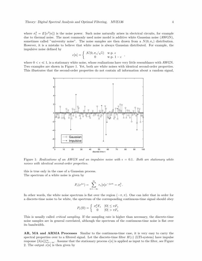
where σ2e = Ee2[n] is the noise power. Such noise naturally arises in electrical circuits, for example

due to thermal noise. The most commonly used noise model is additive white Gaussian noise (AWGN),sometimes called ”university noise”. The noise samples are then drawn from a N(0, σe) distribution.However, it is a mistake to believe that white noise is always Gaussian distributed. For example, theimpulsive noise defined by

e[n] =

N (0, σe/

√ε) w.p. ε

0 w.p. 1− ε ,

where 0 < ε 1, is a stationary white noise, whose realizations have very little resemblance with AWGN.Two examples are shown in Figure 1. Yet, both are white noises with identical second-order properties.This illustrates that the second-order properties do not contain all information about a random signal,

0 10 20 30 40 50 60 70 80 90 100−8

−6

−4

−2

0

2

4

6

8

discrete time n

Gaussian

Impulsive

Figure 1: Realizations of an AWGN and an impulsive noise with ε = 0.1. Both are stationary whitenoises with identical second-order properties.

this is true only in the case of a Gaussian process.The spectrum of a white noise is given by

Pe(ejω) =

∞∑n=−∞

re[n]e−jωn = σ2e .

In other words, the white noise spectrum is flat over the region (−π, π). One can infer that in order fora discrete-time noise to be white, the spectrum of the corresponding continuous-time signal should obey

Pe(Ω) =

σ2eFs |Ω| ≤ πFs0 |Ω| > πFs

This is usually called critical sampling. If the sampling rate is higher than necessary, the discrete-timenoise samples are in general correlated, although the spectrum of the continuous-time noise is flat overits bandwidth.

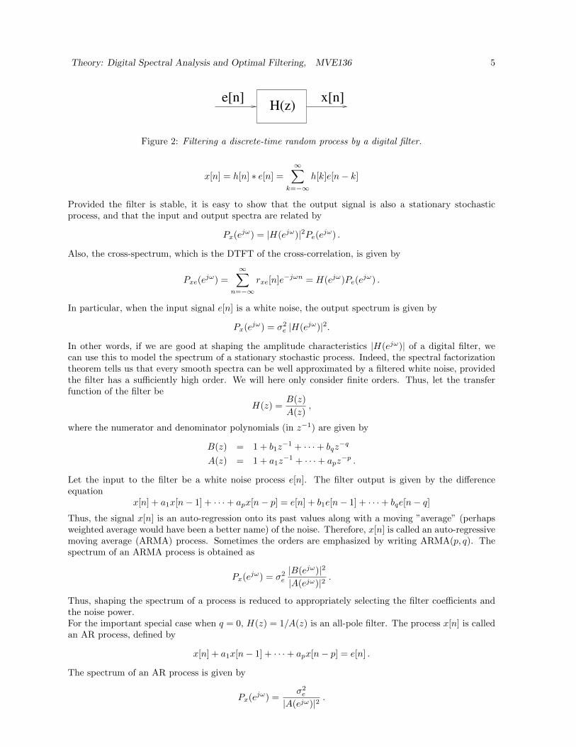
AR, MA and ARMA Processes Similar to the continuous-time case, it is very easy to carry thespectral properties over to a filtered signal. Let the discrete-time filter H(z) (LTI-system) have impulseresponse h[n]∞n=−∞. Assume that the stationary process e[n] is applied as input to the filter, see Figure2. The output x[n] is then given by


x[n]e[n]H(z)

Figure 2: Filtering a discrete-time random process by a digital filter.

x[n] = h[n] ∗ e[n] =

∞∑k=−∞

h[k]e[n− k]

Provided the filter is stable, it is easy to show that the output signal is also a stationary stochasticprocess, and that the input and output spectra are related by

Px(ejω) = |H(ejω)|2Pe(ejω) .

Also, the cross-spectrum, which is the DTFT of the cross-correlation, is given by

Pxe(ejω) =

∞∑n=−∞

rxe[n]e−jωn = H(ejω)Pe(ejω) .

In particular, when the input signal e[n] is a white noise, the output spectrum is given by

Px(ejω) = σ2e |H(ejω)|2.

In other words, if we are good at shaping the amplitude characteristics |H(ejω)| of a digital filter, wecan use this to model the spectrum of a stationary stochastic process. Indeed, the spectral factorizationtheorem tells us that every smooth spectra can be well approximated by a filtered white noise, providedthe filter has a sufficiently high order. We will here only consider finite orders. Thus, let the transferfunction of the filter be

H(z) =B(z)

A(z),

where the numerator and denominator polynomials (in z−1) are given by

B(z) = 1 + b1z−1 + · · ·+ bqz

−q

A(z) = 1 + a1z−1 + · · ·+ apz

−p .

Let the input to the filter be a white noise process e[n]. The filter output is given by the differenceequation

x[n] + a1x[n− 1] + · · ·+ apx[n− p] = e[n] + b1e[n− 1] + · · ·+ bqe[n− q]Thus, the signal x[n] is an auto-regression onto its past values along with a moving ”average” (perhapsweighted average would have been a better name) of the noise. Therefore, x[n] is called an auto-regressivemoving average (ARMA) process. Sometimes the orders are emphasized by writing ARMA(p, q). Thespectrum of an ARMA process is obtained as

Px(ejω) = σ2e

|B(ejω)|2

|A(ejω)|2.

Thus, shaping the spectrum of a process is reduced to appropriately selecting the filter coefficients andthe noise power.For the important special case when q = 0, H(z) = 1/A(z) is an all-pole filter. The process x[n] is calledan AR process, defined by

x[n] + a1x[n− 1] + · · ·+ apx[n− p] = e[n] .

The spectrum of an AR process is given by

Px(ejω) =σ2e

|A(ejω)|2.


Similarly, when p = 0, H(z) = B(z) has only zeros and we get the MA process

x[n] = e[n] + b1e[n− 1] + · · ·+ bqe[n− q]

withPx(ejω) = σ2

e |B(ejω)|2.

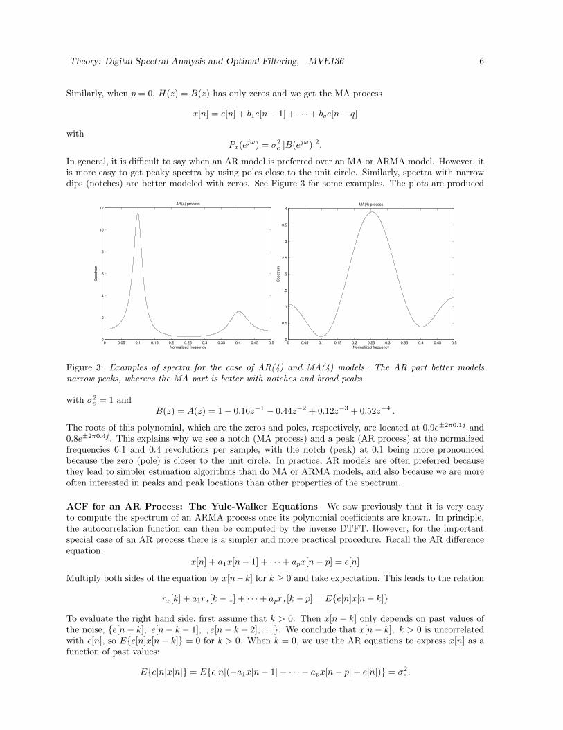
In general, it is difficult to say when an AR model is preferred over an MA or ARMA model. However, itis more easy to get peaky spectra by using poles close to the unit circle. Similarly, spectra with narrowdips (notches) are better modeled with zeros. See Figure 3 for some examples. The plots are produced

0 0.05 0.1 0.15 0.2 0.25 0.3 0.35 0.4 0.45 0.50

2

4

6

8

10

12

Spectr

um

AR(4) process

Normalized frequency0 0.05 0.1 0.15 0.2 0.25 0.3 0.35 0.4 0.45 0.5

0

0.5

1

1.5

2

2.5

3

3.5

4

Sp

ectr

um

Normalized frequency

MA(4) process

Figure 3: Examples of spectra for the case of AR(4) and MA(4) models. The AR part better modelsnarrow peaks, whereas the MA part is better with notches and broad peaks.

with σ2e = 1 and

B(z) = A(z) = 1− 0.16z−1 − 0.44z−2 + 0.12z−3 + 0.52z−4 .

The roots of this polynomial, which are the zeros and poles, respectively, are located at 0.9e±2π0.1j and0.8e±2π0.4j . This explains why we see a notch (MA process) and a peak (AR process) at the normalizedfrequencies 0.1 and 0.4 revolutions per sample, with the notch (peak) at 0.1 being more pronouncedbecause the zero (pole) is closer to the unit circle. In practice, AR models are often preferred becausethey lead to simpler estimation algorithms than do MA or ARMA models, and also because we are moreoften interested in peaks and peak locations than other properties of the spectrum.

ACF for an AR Process: The Yule-Walker Equations We saw previously that it is very easyto compute the spectrum of an ARMA process once its polynomial coefficients are known. In principle,the autocorrelation function can then be computed by the inverse DTFT. However, for the importantspecial case of an AR process there is a simpler and more practical procedure. Recall the AR differenceequation:

x[n] + a1x[n− 1] + · · ·+ apx[n− p] = e[n]

Multiply both sides of the equation by x[n−k] for k ≥ 0 and take expectation. This leads to the relation

rx[k] + a1rx[k − 1] + · · ·+ aprx[k − p] = Ee[n]x[n− k]

To evaluate the right hand side, first assume that k > 0. Then x[n − k] only depends on past values ofthe noise, e[n − k], e[n − k − 1], , e[n − k − 2], . . . . We conclude that x[n − k], k > 0 is uncorrelatedwith e[n], so Ee[n]x[n− k] = 0 for k > 0. When k = 0, we use the AR equations to express x[n] as afunction of past values:

Ee[n]x[n] = Ee[n](−a1x[n− 1]− · · · − apx[n− p] + e[n]) = σ2e .


Thus we have proved the relation

rx[k] +

p∑l=1

alrx[k − l] = σ2e δ[k] , k ≥ 0 , (2)

where δ[k] = 0 for k 6= 0 and δ[0] = 1. The relation (2), for k = 0, 1, . . . , p is known as the Yule-Walker(YW) equations. Since this is a linear relation between the AR coefficients and the autocorrelationfunction, it can be used to efficiently solve for one given the other. If the autocorrelation function isgiven, we can put the equation for k = 1, 2, . . . , N on matrix form as:

rx[0] rx[1] · · · rx[p− 1]rx[1] rx[0] · · · rx[p− 2]

......

. . ....

rx[p− 1] rx[p− 2] · · · rx[0]

a1

a2

...ap

= −

rx[1]rx[2]

...rx[p]

. (3)

This linear system of equations is usually referred to as the Normal Equations. We can express the matrixequation as

Rxa = −rx ,where Rx is called the autocorrelation matrix (of size p×p). The solution w.r.t. a = [a1, a2, . . . , ap]

T nowfollows as a = −R−1

x rx. In practice, more efficient methods for computing a are often used, in particularif p is large and/or if Rx is nearly singular.Conversely, if ak, k = 1, 2, · · · , p and σ2

e are known in advance, then we can use the same set of Yule-Walker equations to solve for rx[k], k = 0, 1, · · · , p. For example, when p = 2 we get 1 a1 a2

a1 1 + a2 0a2 a1 1

rx[0]rx[1]rx[2]

=

σ2e

00

which can easily be solved for (rx[0], rx[1], rx[2])T .

Example 3.1 ACF of an AR(2) processWe demonstrate the Yule-Walker procedure by computing the auto-correlation function for the signalmodel

x[n]− 1.5x[n− 1] + 0.7x[n− 2] = e[n] ,

where σ2e = 1. The relation between the auto-correlation and the AR coefficients given above is in this

case: 1 −1.5 0.7−1.5 1.7 00.7 −1.5 1

rx[0]rx[1]rx[2]

=

100

Solving the linear system gives

rx[0] ≈ 8.85 , rx[±1] ≈ 7.81 , rx[±2] ≈ 5.52

The auto-correlation function at higher lags are computed recursively by

rx[k] = 1.5rx[k − 1]− 0.7rx[k − 2] , k > 0

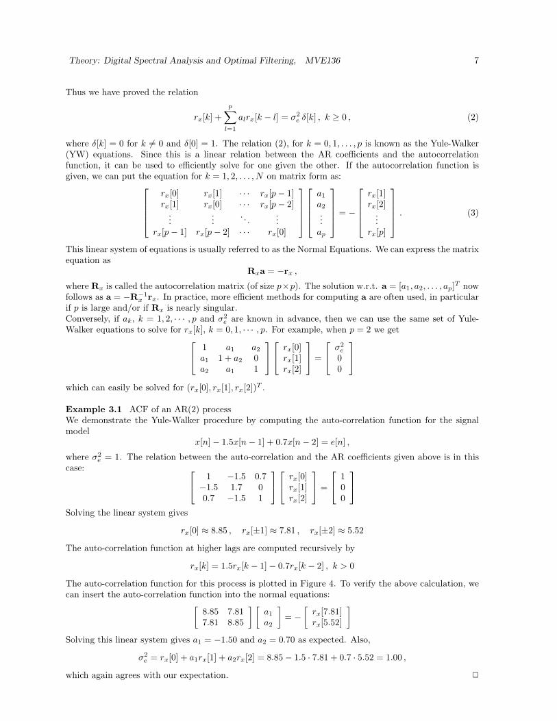
The auto-correlation function for this process is plotted in Figure 4. To verify the above calculation, wecan insert the auto-correlation function into the normal equations:[

8.85 7.817.81 8.85

] [a1

a2

]= −

[rx[7.81]rx[5.52]

]Solving this linear system gives a1 = −1.50 and a2 = 0.70 as expected. Also,

σ2e = rx[0] + a1rx[1] + a2rx[2] = 8.85− 1.5 · 7.81 + 0.7 · 5.52 = 1.00 ,

which again agrees with our expectation. 2


0 5 10 15 20 25 30−4

−2

0

2

4

6

8

10

lag k

Au

to−

co

rre

latio

n r

x[k

]

Auto−correlation for an AR(2) process

Figure 4: Auto-correlation function for the AR(2) process x[n]− 1.5x[n− 1] + 0.7x[n− 2] = e[n].

ACF for MA and ARMA Processes Also in the case of a pure MA process, the auto-correlationfunction is easy to compute. Consider the MA model:

x[n] = e[n] + b1e[n− 1] + · · ·+ bqe[n− q]

To obtain the variance rx[0], just square both sides of the equation and take expectation:

Ex2[n] = rx[0] = E(e[n] + b1e[n− 1] + · · ·+ bqe[n− q])(e[n] + b1e[n− 1] + · · ·+ bqe[n− q])= (1 + b21 + · · · b2q)σ2

e

where we have used that e[n] is white noise. For rx[1], multiply the MA equation by x[n − 1] and takeexpectation:

rx[1] = E(e[n] + b1e[n− 1] + · · ·+ bqe[n− q])(e[n− 1] + b1e[n− 2] + · · ·+ bqe[n− q − 1])= (b1 + b2b1 + · · · bqbq−1)σ2

e .

The same principle is used to compute rx[k], k = 2, 3, . . . , noting that rx[k] = 0 for k > q. Thus, an MAprocess has a finite correlation length, given by its order q. Note that although we can easily computethe auto-correlation function given the MA coefficients and the noise variance, the converse is in generalnot as simple. This is because the relation between rx[k] and the bk:s is not linear as in the case of an ARprocess. From the above we see that it is a quadratic relation. Although this may sound simple enough,a computationally efficient and robust (to errors in rx[k]) method to compute an MA model bkqk=1, σ

2e

from the auto-correlation coefficients rx[k]qk=0 is not known to date. The reader is referred to [3, 4] forapproximate methods with acceptable computational cost and statistical properties.

Example 3.2 ACF of an MA(2) processConsider the second-order MA process:

y[n] = e[n]− 1.5e[n− 1] + 0.5e[n− 2] ,

where e[n] is WGN with Ee2[n] = σ2e . By direct calculation we get

Ey2[n] = E(e[n]− 1.5e[n− 1] + 0.5e[n− 2])(e[n]− 1.5e[n− 1] + 0.5e[n− 2])= Ee2[n]+ E(−1.5e[n− 1])2+ E(0.5e[n− 2])2= σ2

e + 1.52σ2e + 0.52σ2

e = 3.5σ2e .


Similarly,

Ey[n]y[n− 1] = E(e[n]− 1.5e[n− 1] + 0.5e[n− 2])(e[n− 1]− 1.5e[n− 2] + 0.5e[n− 3])= E−1.5e2[n− 1]+ E(0.5×−1.5)e2[n− 2]= −1.5σ2

e − 0.75σ2e = −2.25σ2

e

and

Ey[n]y[n− 2] = E(e[n]− 1.5e[n− 1] + 0.5e[n− 2])(e[n− 2]− 1.5e[n− 3] + 0.5e[n− 4])= E0.5e2[n− 2] = 0.5σ2

e .

Thus, the ACF is given by

ry[k] =

3.5σ2

e , k = 0−2.25σ2

e , k = ±10.5σ2

e , k = ±20 , |k| > 2

.

2

Computing the auto-correlation function for an ARMA process requires in general considerably moreeffort than in the pure AR or MA cases. A common way to solve this problem is to exploit that theauto-correlation is the inverse transform of the spectrum, which for an ARMA model is given by:

Px(ejω) = σ2e

|B(ejω)|2

|A(ejω)|2.

The inverse transform is

rx[n] =1

2π

π∫−π

Px(ejω)ejωndω ,

and the integral can be solved using calculus of residues. For low model orders, especially when the rootsof A(z) are real-valued, it is easier to use the inverse Z-transform:

rx[n] = Z−1Px(z) = Z−1

σ2e

B(z)B(z−1)

A(z)A(z−1)

.

For simple cases, the inverse transform can be carried out using partial fraction expansion (with longdivision if q ≥ p) and table lookup. For the special case of an ARMA(1,1)-process, there is an evensimpler procedure. Consider the model

x[n] + a1x[n− 1] = e[n] + b1e[n− 1]

First, square both sides of the equation and take expectation, yielding

rx[0](1 + a21) + 2a1rx[1] = (1 + b21)σ2

e

Next, multiply the ARMA(1,1) equation by x[n− 1] and take expectation. This gives

rx[1] + a1rx[0] = 0 + b1σ2e ,

where we have used that x[n− 1] is uncorrelated with e[n] and that Ee[n− 1]x[n− 1] = σ2e . We now

have two equations in the two unknowns rx[0] and rx[1], which can easily be solved given numerical valuesof a1, b1 and σ2

e . To obtain rx[k] for higher lags, multiply the ARMA equation by x[n − k], k > 1 andtake expectation. This gives

rx[k] + a1rx[k − 1] = 0 , k > 1.

Thus, rx[k] can be recursively computed once rx[1] is known. The above relation is known as the extendedYule-Walker equations, and a similar relation is obtained in the general ARMA(p,q) case for lags k > q.This shows that a linear relation between the auto-correlation function and the AR parameters akcan be obtained also in the ARMA case. However, the auto-correlation coefficients are still non-linearfunctions of the MA parameters bk.


Spectral Lines By spectral factorization, any smooth spectrum can be well approximated by an ARMAprocess of sufficiently high order. But what about spectra that are not smooth? The so-called Wolddecomposition tells us that all stationary stochastic processes (i.e. even those with non-smooth spectra)can be decomposed into a ”purely” stochastic part and a perfectly predictable part. The stochastic partis represented as an ARMA model as before. The remaining part is represented as a sum of sinusoids:

s[n] =

p∑k=1

Ak cos(ωkn+ φk) .

The frequencies ωk and the amplitudes Ak are usually regarded as deterministic (fixed), whereas theinitial phases φk are modeled as independent and uniformly distributed in (0, 2π). It is then easy to showthat s[n] in fact becomes a stationary stochastic process with zero mean and autocorrelation function

rs[k] =

p∑k=1

A2k

2cos(ωkn) .

Although s[n] is formally a stochastic process, it is clear that we can perfectly predict the future valuesof s[n] if we only know sufficiently many initial conditions. The interested reader can show that both s[n]and rs[n] obey the following homogenous difference equation of order 2p:

s[n] + a1s[n− 1] + · · ·+ a2ps[n− 2p] = 0 ,

where the corresponding polynomial A(z) has its roots on the unit circle, at e±jωkpk=1.Taking the DTFT of rs[k], the spectrum is obtained as

Ps(ejω) =

π

2

p∑k=1

A2k δ(ω − ωk) + δ(ω + ωk) .

In other words, the spectrum consists of infinitely narrow spectral peaks, located at the frequencies ±ωk.We get peaks also at the negative frequencies, because cosωn = (ejωn+e−jωn)/2 consists of two ”phasors”rotating in opposite directions. The angular speed of these phasors are the frequencies.

4 Digital Spectral Analysis

We have previously argued that the spectrum of a bandlimited continuous-time signal x(t) can in princi-ple be inferred from its discrete-time samples x[n]. However, computing the spectrum involves averagingover infinitely many realizations of the signal. In practice, one has usually access to only one realization.Fortunately, for a well-behaved stationary signal, we can replace ensemble averaging by time averaging(ergodicity). Thus, given an infinite observation time, the spectrum of a signal could be perfectly es-timated. In practice, the data length is limited by the available time to deliver a result, the computerprocessor speed and memory size, and/or the time over which the process can be considered stationary.Thus, the problem of spectral estimation is to estimate the spectrum Px(ejω) based on a finite samplex[0], x[1], . . . , x[N − 1]. The number of data required will depend on the demanded accuracy as well asthe nature of the true spectrum. It is also different for different methods as we shall see.

4.1 Non-Parametric Methods

The simplest and most straightforward way to estimate the power spectrum of a signal is to use non-parametric methods, also known as Fourier-based (or window-based) methods. The main advantagesof these methods are that 1) they do not require specification of a signal model, and 2) they are easyto implement and computationally inexpensive due to the efficient fast Fourier transform (FFT). Thedisadvantage is that the frequency resolution is limited by the length of the observation time.


The Periodogram

The classical approach to spectral estimation is to use the so-called periodogram. For a given datasequence x[n], n = 0, 1, · · · , N − 1, the periodogram is the normalized magnitude square of the DTFT:

Pper(ejω) =

1

N|XN (ejω)|2 (4)

XN (ejω) =

N−1∑n=0

x[n]e−jωn (5)

We remember from the deterministic Signals and Systems theory that the finite-interval DTFT (andhence the periodogram) has a limited frequency resolution. Two spectral peaks that are spaced less than∆ω ≈ 2π/N apart will show up as a single peak in Pper(e

jω). Still, smoother parts of the spectrum of adeterministic signal will generally be well approximated by the periodogram. Unfortunately, this is notthe case when x[n] is stochastic. The periodogram will then reflect the spectral contents of the particularrealization of x[n] that has been observed. In general, we are more interested in the average behavior,given by the ”true” spectrum (1). To connect the two, it is useful to rewrite (4) in the form

Pper(ejω) =

N−1∑k=−N+1

rx[k]e−jω (6)

where rx[k] is the sample autocorrelation function

rx[k] =1

N

N−1∑n=k

x[n]x[n− k] .

The interested reader is encouraged to prove the equivalence of (4) and (6). It is now easy to show that

limN→∞

EPper(ejω) = Px(ejω)

which shows that the periodogram is an asymptotically unbiased estimator. Under some regularityconditions, it is further possible to show [3] that

E(Pper(ejω)− Px(ejω))2 = P 2x (ejω) +RN ,

where the reminder term RN tends to zero as N →∞. Thus, the standard deviation of the periodogramis approximately as large as the quantity (the spectrum) it is supposed to estimate. In its basic form, theperiodogram is apparently an unacceptably noisy estimator. Fortunately, there are modifications withmuch better behavior.

The Modified Periodogram

The DTFT has a limited resolution, due to the inherent windowing of the data. We can express theDTFT as

XN (ejω) =

∞∑n=−∞

wR[n]x[n]e−jωn ,

where wR[n] is the length-N rectangular window

wR[n] =

1 0 ≤ n ≤ N − 10 otherwise

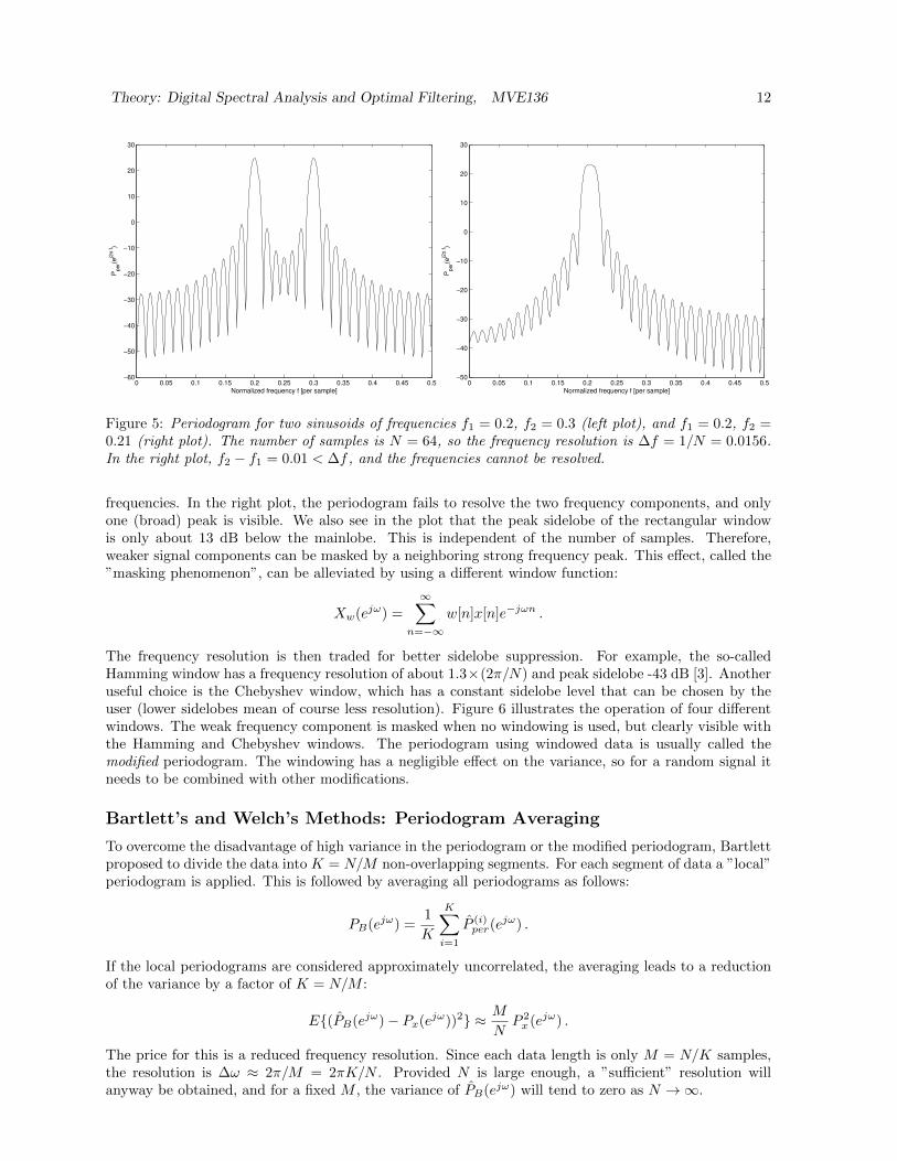
Window functions are usually characterized in the frequency domain in terms of the mainlobe width ∆ωand the peak sidelobe level. Among all windows of a given length, the rectangular has the smallest ∆ω,given by ∆ω = 2π/N (radians/sample). Figure 5 shows the periodogram for two sinusoids of differentfrequencies. In the left plot, the sinusoids are well separated, and two peaks are clearly seen at the right


0 0.05 0.1 0.15 0.2 0.25 0.3 0.35 0.4 0.45 0.5−60

−50

−40

−30

−20

−10

0

10

20

30

Normalized frequency f [per sample]

Pp

er(e

j2π f)

0 0.05 0.1 0.15 0.2 0.25 0.3 0.35 0.4 0.45 0.5−50

−40

−30

−20

−10

0

10

20

30

Normalized frequency f [per sample]

Pp

er(e

j2π f)

Figure 5: Periodogram for two sinusoids of frequencies f1 = 0.2, f2 = 0.3 (left plot), and f1 = 0.2, f2 =0.21 (right plot). The number of samples is N = 64, so the frequency resolution is ∆f = 1/N = 0.0156.In the right plot, f2 − f1 = 0.01 < ∆f , and the frequencies cannot be resolved.

frequencies. In the right plot, the periodogram fails to resolve the two frequency components, and onlyone (broad) peak is visible. We also see in the plot that the peak sidelobe of the rectangular windowis only about 13 dB below the mainlobe. This is independent of the number of samples. Therefore,weaker signal components can be masked by a neighboring strong frequency peak. This effect, called the”masking phenomenon”, can be alleviated by using a different window function:

Xw(ejω) =

∞∑n=−∞

w[n]x[n]e−jωn .

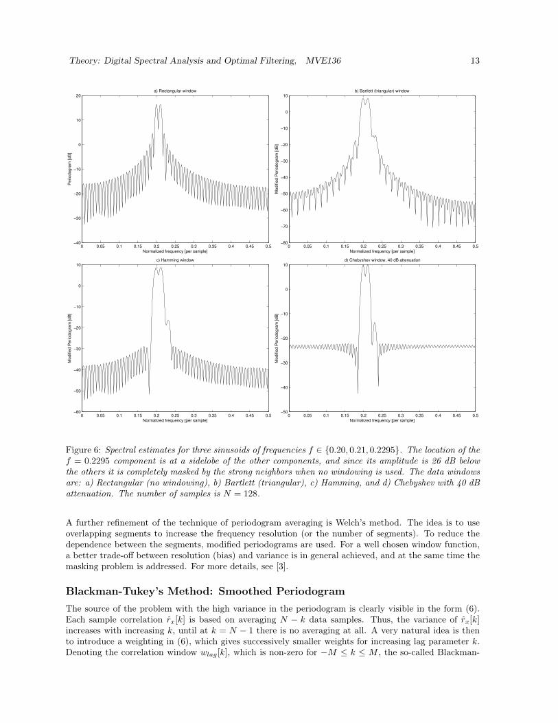
The frequency resolution is then traded for better sidelobe suppression. For example, the so-calledHamming window has a frequency resolution of about 1.3×(2π/N) and peak sidelobe -43 dB [3]. Anotheruseful choice is the Chebyshev window, which has a constant sidelobe level that can be chosen by theuser (lower sidelobes mean of course less resolution). Figure 6 illustrates the operation of four differentwindows. The weak frequency component is masked when no windowing is used, but clearly visible withthe Hamming and Chebyshev windows. The periodogram using windowed data is usually called themodified periodogram. The windowing has a negligible effect on the variance, so for a random signal itneeds to be combined with other modifications.

Bartlett’s and Welch’s Methods: Periodogram Averaging

To overcome the disadvantage of high variance in the periodogram or the modified periodogram, Bartlettproposed to divide the data into K = N/M non-overlapping segments. For each segment of data a ”local”periodogram is applied. This is followed by averaging all periodograms as follows:

PB(ejω) =1

K

K∑i=1

P (i)per(e

jω) .

If the local periodograms are considered approximately uncorrelated, the averaging leads to a reductionof the variance by a factor of K = N/M :

E(PB(ejω)− Px(ejω))2 ≈ M

NP 2x (ejω) .

The price for this is a reduced frequency resolution. Since each data length is only M = N/K samples,the resolution is ∆ω ≈ 2π/M = 2πK/N . Provided N is large enough, a ”sufficient” resolution willanyway be obtained, and for a fixed M , the variance of PB(ejω) will tend to zero as N →∞.


0 0.05 0.1 0.15 0.2 0.25 0.3 0.35 0.4 0.45 0.5−40

−30

−20

−10

0

10

20a) Rectangular window

Pe

rio

do

gra

m [

dB

]

Normalized frequency [per sample]

0 0.05 0.1 0.15 0.2 0.25 0.3 0.35 0.4 0.45 0.5−80

−70

−60

−50

−40

−30

−20

−10

0

10b) Bartlett (triangular) window

Mo

difie

d P

erio

do

gra

m [

dB

]


0 0.05 0.1 0.15 0.2 0.25 0.3 0.35 0.4 0.45 0.5−60

−50

−40

−30

−20

−10

0

10c) Hamming window

Mo

difie

d P

erio

do

gra

m [

dB

]


0 0.05 0.1 0.15 0.2 0.25 0.3 0.35 0.4 0.45 0.5−50

−40

−30

−20

−10

0

10d) Chebyshev window, 40 dB attenuation

Mo

difie

d P

erio

do

gra

m [

dB

]


Figure 6: Spectral estimates for three sinusoids of frequencies f ∈ 0.20, 0.21, 0.2295. The location of thef = 0.2295 component is at a sidelobe of the other components, and since its amplitude is 26 dB belowthe others it is completely masked by the strong neighbors when no windowing is used. The data windowsare: a) Rectangular (no windowing), b) Bartlett (triangular), c) Hamming, and d) Chebyshev with 40 dBattenuation. The number of samples is N = 128.

A further refinement of the technique of periodogram averaging is Welch’s method. The idea is to useoverlapping segments to increase the frequency resolution (or the number of segments). To reduce thedependence between the segments, modified periodograms are used. For a well chosen window function,a better trade-off between resolution (bias) and variance is in general achieved, and at the same time themasking problem is addressed. For more details, see [3].

Blackman-Tukey’s Method: Smoothed Periodogram

The source of the problem with the high variance in the periodogram is clearly visible in the form (6).Each sample correlation rx[k] is based on averaging N − k data samples. Thus, the variance of rx[k]increases with increasing k, until at k = N − 1 there is no averaging at all. A very natural idea is thento introduce a weighting in (6), which gives successively smaller weights for increasing lag parameter k.Denoting the correlation window wlag[k], which is non-zero for −M ≤ k ≤ M , the so-called Blackman-


Tukey estimate is given by

PBT (ejω) =

M∑k=−M

wlag[k]rx[k]e−jkω . (7)

The original periodogram is retrieved if M = N and a rectangular window is used. An appealinginterpretation of PBT (ejω) is obtained by looking at (7) as the DTFT of wlag[k]rx[k]:

PBT (ejω) =

∞∑k=−∞

wlag[k]rx[k]e−jkω = DTFTwlag[k]rx[k]

(since wlag[k] = 0 for |k| > M). Multiplication in the time domain corresponds to convolution in thefrequency domain, so we can also write

PBT (ejω) =1

2πWlag(e

jω) ∗ Pper(ejω) =1

2π

π∫−π

Pper(ej(ω−ξ))Wlag(e

jξ)dξ ,

where Wlag(ejω) is the DTFT of the window function and Pper(e

jω) is the periodogram, which is the

DTFT of rx[k]. Thus, PBT (ejω) is in effect a smoothed periodogram. Think of Wlag(ejω) as a rectangular

box of size ∆ω. Then, the BT (Blackman-Tukey) spectral estimate at a certain frequency ω is obtainedby a local averaging (=smoothing) of the periodogram, in the interval (ω−∆ω/2, ω+∆ω/2). In practice,the window function has a non-rectangular mainlobe which implies some weighted averaging, and alsosidelobes which may result in frequency masking.It is clear that the smoothing reduces the variance, at the price of a reduced frequency resolution (bias).It can be shown that (e.g. [3])

EPBT (ejω) ≈ 1

2πPx(ejω) ∗Wlag(e

jω)

E(PBT (ejω)− Px(ejω))2 ≈ 1

N

M∑k=−M

w2lag[k]P 2

x (ejω)

Given these formulas, the length and the shape of the lag window is selected as a tradeoff between thevariance and the bias of the estimate. For M → ∞, the Fourier transform of the lag window becomesmore and more like a Dirac pulse, and the BT estimate becomes unbiased. In practice, M should bechosen large enough so that all details in the spectrum can be recovered (which of course depends on theshape of the true spectrum), but yet M N to reduce the variance. In general, the BT method givesthe best trade-off among the non-parametric spectral estimation methods presented here.

Example 4.1 Non-Parametric Spectral EstimationA set of N = 1000 data samples were generated according to the AR model

x[n]− 1.5x[n− 1] + 0.7x[n− 2] = e[n] ,

where e[n] is N (0, 1) white noise. Figure 7, left plot, shows the true spectrum along with the Periodogramestimate. It is clear that the Periodogram is a very noise estimate of the spectrum, although ”on average”it looks OK. In Figure 7, right plot, the BT spectrum estimate is shown for various lengths M of the lagwindow. A Hamming window is used. It is clear that reducing M lowers the variance of the estimate atthe price of a reduced resolution. In this case, M ∈ (20, 50) appears to be a good choice. 2

4.2 Parametric Spectral Estimation

As we previously saw, non-parametric spectral estimation methods have limitations in terms of frequencyresolution and estimation variance. An attempt to overcome these limitations is to use parametricmodeling of the measured signal. Such methods are expected to perform much better when the ”true”spectrum can be well approximated with a model using few parameters in the chosen model class. Thisis because the variance of the estimated spectrum is in general proportional to the number of estimatedparameters. We shall only consider signals with AR models in this review (for other models, see e.g.[3, 4]).


0 0.05 0.1 0.15 0.2 0.25 0.3 0.35 0.4 0.45 0.50

50

100

150

Normalized Frequency

Sp

ectr

um

Periodogram

True spectrum

Periodogram

0 0.05 0.1 0.15 0.2 0.25 0.3 0.35 0.4 0.45 0.50

10

20

30

40

50

60


Sp

ectr

um

Blackman−Tukey Spectrum Estimation

True spectrum

M=20

M=50

M=100

Figure 7: Examples of non-parametric spectrum estimation using the Periodogram (left plot) and theBlackman-Tukey method (right plot). The true spectrum is an AR(2) process.

AR Models

In an AR(p) model, the data sample at time n is assumed to be the weighted combination of the previousdata samples x[n− k], k = 1, . . . , p, and a ”driving” white noise e[n],

x[n] = −p∑k=1

akx[n− k] + e[n] .

This is equivalent to x[n] being the output of an all-pole system H(z) = 1/A(z), whose input is the whitenoise e[n]. Given the above model, the spectrum of x[n] is represented as

Px(ejω) =σ2e

|A(ejω)|2.

Therefore, the spectral estimation is now reduced to selecting the model order p, finding the modelparameters akk=1p, and estimating the innovation variance σ2

e . Now, recall the normal equations (3).Given measured data x[n]N−1

n=0 , a natural idea is to replace the true (but unknown) autocorrelationsrx[k] in (3) with the sample autocorrelations:

rx[k] =1

N

N−1∑n=k

x[n]x[n− k] , k = 0, 1, . . . , p .

The sample version of the normal equations are now expressed asrx[0] rx[1] · · · rx[p− 1]rx[1] rx[0] · · · rx[p− 2]

......

. . ....

rx[p− 1] rx[p− 2] · · · rx[0]

a1

a2

...ap

= −

rx[1]rx[2]

...rx[p]

The solution is given by a = −R−1

x rx with obvious notation. Several numerically efficient algorithmsexist for computing the estimate, including the so-called Levinson-type recursions, see [3]. However, forour purposes, it suffices to type a=-R\r in Matlab, or use a suitable command from the Signal Processingor System Identification toolboxes.Once the AR parameters are estimated, the noise variance is computed using (2) for k = 0, leading to

σ2e = rx[0] +

p∑k=1

alrx[k] .


Several methods have been proposed to estimate the model order p. The basic idea of most methods isto compute the noise variance σ2

e for increasing values of p = 1, 2, . . . , and observe the decrease of theresidual noise power. When the ”true” order has been found (if there is one), the noise power is expectedto level out, i.e. further increase of p does not yield any significant decrease of σ2

e . The difference amongthe various suggested methods lies in determining what to mean by a ”significant” decrease. See, e.g.,[4] for details.

Example 4.2 AR Spectral EstimationConsider the same AR(2) model as in Example 4.1. For the same N = 1000 samples, the sample auto-correlation function was calculated to

rx[0] = 7.74 , rx[1] = 6.80 , rx[2] = 4.75 .

Solving the YW equations for the AR parameters (assuming the correct model order p = 2 is known)then gives a1 = −1.50, a2 = 0.70, which in fact agrees with the true parameters up to the given precision.The estimated noise variance is found to be

σ2e = 7.74− 1.50 · 6.80 + 0.70 · 4.75 = 0.87 ,

which is slightly too low. The resulting YW-based spectrum estimate is displayed in Figure 8. It isremarked that the pyulear command in Matlab gives a spectrum estimate with the same shape, but thelevel is too low. 2

0 0.05 0.1 0.15 0.2 0.25 0.3 0.35 0.4 0.45 0.50

10

20

30

40

50

60


Sp

ectr

um

True spectrum

AR spectral estimate

Figure 8: Parametric AR spectral estimation using the YW method. Both the estimated and the truespectrum is an AR(2) model.

In the above example, the YW method is applied to data that are generated according to an AR modelwith known order. As one could expect, the resulting spectrum estimate agrees very well with the truespectrum. With measured data, it is of course never the case that an AR model can give a perfectdescription of the true spectrum. The best one can hope for is that a ”sufficiently good” approximationcan be found using a not too high model order. It this is the case, the parametric AR-based spectrumestimate will in general give better performance than the non-parametric methods, particularly for shortdata records (N small).

5 Optimal Filtering

One of the main tasks in digital signal processing is to estimate signals (or parameters of signals) fromnoise corrupted measurements. For example, background noise can disturb a recorded speech signal


so that it becomes unintelligible, or an image taken from an infrared camera shows thermal noise thatsignificantly reduces the image quality. The noise is often modeled as additive, although in many casesthere are also other distortions, including filtering (”blurring”) and phase-noise, which is multiplicative.Assuming additive noise, the measured signal x[n] can be described as a stochastic process,

x[n] = s[n] + w[n]

where s[n] denotes the signal of interest and w[n] is the noise (or disturbance). The optimal filtering

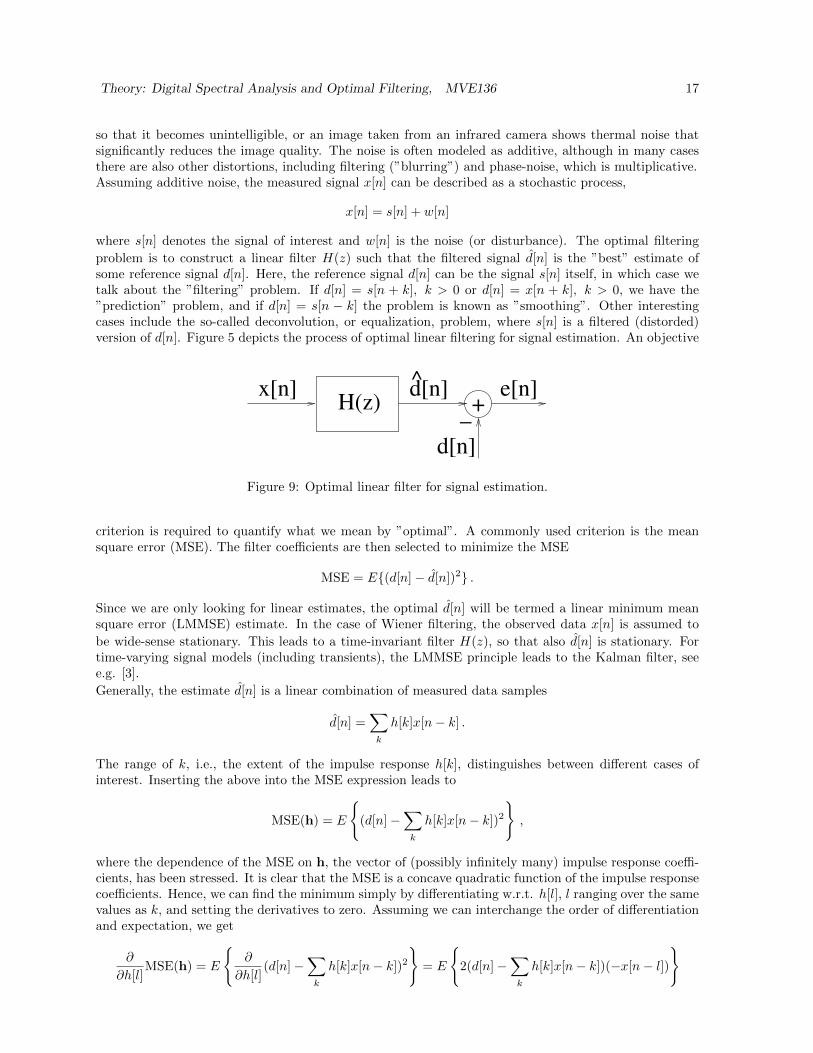
problem is to construct a linear filter H(z) such that the filtered signal d[n] is the ”best” estimate ofsome reference signal d[n]. Here, the reference signal d[n] can be the signal s[n] itself, in which case wetalk about the ”filtering” problem. If d[n] = s[n + k], k > 0 or d[n] = x[n + k], k > 0, we have the”prediction” problem, and if d[n] = s[n − k] the problem is known as ”smoothing”. Other interestingcases include the so-called deconvolution, or equalization, problem, where s[n] is a filtered (distorded)version of d[n]. Figure 5 depicts the process of optimal linear filtering for signal estimation. An objective

x[n]H(z)

d[n] e[n]^

_

d[n]

+

Figure 9: Optimal linear filter for signal estimation.

criterion is required to quantify what we mean by ”optimal”. A commonly used criterion is the meansquare error (MSE). The filter coefficients are then selected to minimize the MSE

MSE = E(d[n]− d[n])2 .

Since we are only looking for linear estimates, the optimal d[n] will be termed a linear minimum meansquare error (LMMSE) estimate. In the case of Wiener filtering, the observed data x[n] is assumed to

be wide-sense stationary. This leads to a time-invariant filter H(z), so that also d[n] is stationary. Fortime-varying signal models (including transients), the LMMSE principle leads to the Kalman filter, seee.g. [3].

Generally, the estimate d[n] is a linear combination of measured data samples

d[n] =∑k

h[k]x[n− k] .

The range of k, i.e., the extent of the impulse response h[k], distinguishes between different cases ofinterest. Inserting the above into the MSE expression leads to

MSE(h) = E

(d[n]−

∑k

h[k]x[n− k])2

,

where the dependence of the MSE on h, the vector of (possibly infinitely many) impulse response coeffi-cients, has been stressed. It is clear that the MSE is a concave quadratic function of the impulse responsecoefficients. Hence, we can find the minimum simply by differentiating w.r.t. h[l], l ranging over the samevalues as k, and setting the derivatives to zero. Assuming we can interchange the order of differentiationand expectation, we get

∂

∂h[l]MSE(h) = E

∂

∂h[l](d[n]−

∑k

h[k]x[n− k])2

= E

2(d[n]−

∑k

h[k]x[n− k])(−x[n− l])


Evaluating the expectation now yields

∂

∂h[l]MSE(h) = −2rdx[l] + 2

∑k

h[k]rx[l − k]

Equating the derivative to zero shows that the optimal filter coefficients must satisfy∑k

h[k]rx[l − k] = rdx[l] . (8)

This relation, for a suitable range of k and l, is known as the Wiener-Hopf (W-H) equations.

5.1 Causal FIR Wiener Filters

We shall first review case of a causal finite impulse response (FIR) filter. The estimate of d[n] is thenbased on p past samples of x[n]:

d[n] =

p−1∑k=0

h[k]x[n− k]

Thus, H(z) is the FIR filter

H(z) =

p−1∑k=0

h[k]z−k

For this case, the W-H equations become

p−1∑k=0

h[k]rx[l − k] = rdx[l] , l = 0, 1, . . . , p− 1.

This is a set of p linear equations in the p unknowns h[0], . . . , h[p−1]. The solution is found by expressingthe W-H equations in matrix form:

rx[0] rx[1] · · · rx[p− 1]rx[1] rx[0] · · · rx[p− 2]

......

. . ....

rx[p− 1] rx[p− 2] · · · rx[0]

h[0]h[1]

...h[p− 1]

=

rdx[0]rdx[1]

...rdx[p− 1]

We can express this compactly as Rxh = rdx, and the solution is given by hFIR = R−1

x rdx. This givesthe coefficients of the optimal FIR Wiener filter. The minimum MSE can be shown to be

MSE(hFIR) = rd[0]−p−1∑k=0

rdx[k]hFIR[k] = rd[0]− rTdxhFIR

Once the optimal filter has been found, the best estimate (in the LMMSE sense) is given by

d[n] =

p−1∑k=0

hFIR[k]x[n− k] = hTFIRx[n] .

To find the optimal LMMSE filter requires apparently that the autocorrelation sequence rx[k] and crosscorrelation sequence rdx[k], for k = 0, 1, · · · , p − 1, are known in advance. In many practical situationsthis information is unavailable, and in addition the statistical properties may be (slowly) time-varying.In such a case, it may be possible to apply a so-called adaptive filter, which learns the optimal filtercoefficients from data. In this context, FIR filters are highly useful, since they are always guaranteed tobe stable. Adaptive filtering will be explored in the forthcoming course Applied Signal Processing.


Example 5.1 FIR Wiener FilterSuppose a desired signal d[n] is corrupted by additive noise w[n], so the measured signal x[n] is given byx[n] = d[n] + w[n]. The desired signal is modeled by the AR(1) equation

d[n]− 0.5d[n− 1] = ed[n] ,

whereas the disturbance is modeled by

w[n] + 0.5w[n− 1] = ew[n] .

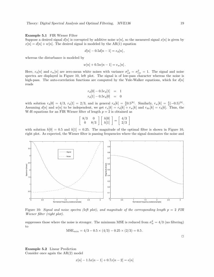
Here, ed[n] and ew[n] are zero-mean white noises with variance σ2ed = σ2

ew = 1. The signal and noisespectra are displayed in Figure 10, left plot. The signal is of low-pass character whereas the noise ishigh-pass. The auto-correlation functions are computed by the Yule-Walker equations, which for d[n]reads

rd[0]− 0.5rd[1] = 1

rd[1]− 0.5rd[0] = 0

with solution rd[0] = 4/3, rd[1] = 2/3, and in general rd[k] = 430.5|k|. Similarly, rw[k] = 4

3 (−0.5)|k|.Assuming d[n] and w[n] to be independent, we get rx[k] = rd[k] + rw[k] and rdx[k] = rd[k]. Thus, theW-H equations for an FIR Wiener filter of length p = 2 is obtained as[

8/3 00 8/3

] [h[0]h[1]

]=

[4/32/3

]with solution h[0] = 0.5 and h[1] = 0.25. The magnitude of the optimal filter is shown in Figure 10,right plot. As expected, the Wiener filter is passing frequencies where the signal dominates the noise and

0 0.5 1 1.5 2 2.5 30

0.5

1

1.5

2

2.5

3

3.5

4

Normalized frequency [radians/sample]

Sp

ectr

um

[lin

ea

r]

Signal

Noise

0 0.5 1 1.5 2 2.5 30

0.1

0.2

0.3

0.4

0.5

0.6

0.7

0.8

0.9

1

Normalized frequency [radians/sample]

Magnitude [lin

ear]

Figure 10: Signal and noise spectra (left plot), and magnitude of the corresponding length p = 2 FIRWiener filter (right plot).

suppresses those where the noise is stronger. The minimum MSE is reduced from σ2w = 4/3 (no filtering)

toMSEmin = 4/3− 0.5× (4/3)− 0.25× (2/3) = 0.5 .

2

Example 5.2 Linear PredictionConsider once again the AR(2) model

x[n]− 1.5x[n− 1] + 0.7x[n− 2] = e[n]


where e[n] is zero-mean white noise with variance σ2e = 1. Suppose we wish to predict the future values

of x[n] based on past observations. We choose an FIR predictor of length p = 2:

x[n+ k] = h[0]x[n] + h[1]x[n− 1] ,

where k > 0. Thus d[n] = x[n+ k] in this case. The coefficients h[0], h[1] should be chosen to minimizethe MSE

MSE(h[0], h[1]) = E(x[n+ k]− x[n+ k])2 .

The WH equations are in this case given by:[rx[0] rx[1]rx[1] rx[0]

] [h[0]h[1]

]=

[rx[k]

rx[k + 1]

]Solving this 2× 2 linear system gives:[

h[0]h[1]

]=

1

r2x[0]− r2

x[1]

[rx[0]rx[k]− rx[1]rx[k + 1]rx[0]rx[k + 1]− rx[1]rx[k]

]The auto-correlation function for the given AR model was calculated in Example 3.1:

rx[0] ≈ 8.85 , rx[1] ≈ 7.81 , rx[2] ≈ 5.52 , rx[3] ≈ 2.81 , rx[4] ≈ 0.35 . . .

Inserting these values into the expression for the optimal filter coefficients yields for k = 1:

h[0], h[1]k=1 = 1.5,−0.7

Thus, the optimal one-step ahead predictor is given by

x[n+ 1] = 1.5x[n]− 0.7x[n− 1] .

This is an intuitively appealing result, as seen by rewriting the AR model as

x[n+ 1] = 1.5x[n]− 0.7x[n− 1] + e[n+ 1] .

At time n we have no information about e[n+ 1], so the best is to replace it with its mean, which is zero.This results in our optimal predictor. The prediction error is in this case simply the white noise e[n+ 1],and the minimum MSE is:

MSEk=1 = 8.85− 1.5 · 7.81 + 0.7 · 5.52 = 1.00

as expected.For k = 3 we get the filter coefficients:

h[0], h[1]k=3 = 1.28,−2.31

The optimal three-step ahead predictor is therefore given by:

x[n+ 3] = 1.28x[n]− 2.31x[n− 1] .

The minimum MSE is now obtained as:

MSEk=3 = 8.85− 1.28 · 2.81 + 2.31 · 0.35 = 6.06 ,

which is considerably higher than for k = 1. This is not surprising; prediction is of course more difficultthe longer the prediction horizon is. 2


5.2 Non-causal IIR Wiener Filters

The FIR filter is limited in the sense that its impulse response is required to be finite. One can expectthat an infinite impulse response (IIR) filter can give more flexibility, and thus smaller MSE. The most

flexible case is when the estimate d[n] is allowed to depend on all possible data:

d[n] =

∞∑k=−∞

h[k]x[n− k]

Thus, H(z) is the non-causal IIR filter

H(z) =

∞∑k=−∞

h[k]z−k

In this case, the W-H equations are infinitely many, and they depend on an infinite set of unknowns:

∞∑k=−∞

h[k]rx[l − k] = rdx[l] , −∞ < l <∞ .

The solution is easily obtained by transforming the W-H equations to the frequency domain. Note thatthe term on the left-hand side is the convolution of h[k] and rx[k]. By taking the Z-transform, this isconverted to multiplication:

H(z)Px(z) = Pdx(z) .

Recall that Px(ejω) is the DTFT of rx[k], so Px(z) is the Z-transform. Likewise, Pdx(z) denotes theZ-transform of the cross-correlation rdx[n]. The optimal non-causal IIR filter is now easily obtained as

Hnc(z) =Pdx(z)

Px(z)

If desired, the impulse response coefficients can be computed by inverse Z-transform.An interesting special case is obtained if x[n] = s[n] + w[n], where s[n] and w[n] are uncorrelated, andd[n] = s[n]. Then, it follows that

Px(z) = Ps(z) + Pw(z) , Pdx(z) = Ps(z) ,

and the non-causal LMMSE estimate becomes (in the DTFT-domain)

Hnc(ejω) =

Ps(ejω)

Ps(ejω) + Pw(ejω)=

SNR(ω)

SNR(ω) + 1,

where SNR(ω) = Ps(ejω)/Pw(ejω) is the Signal-to-Noise Ratio at the frequency ω. The nice interpreta-

tion is that the optimal filter should be Hnc(ejω) ≈ 1 at those frequencies where the SNR is high, and

Hnc(ejω) ≈ 0 where the SNR is poor. When Ps(e

jω) = Pw(ejω), which corresponds to 0 dB SNR, thefilter should have a gain of about -6 dB. Also note that Hnc(e

jω) is purely real in this case, i.e. thereis no phase distortion. This is of course possible only for a non-causal filter. However, in contrast tothe analog case, non-causal digital filters can in fact be implemented in practice, just not in real time.Given a pre-recorded batch of data, the transfer function Hnc(e

jω) can, for example, be applied in thefrequency domain, by first taking the DTFT of x[n]. The filtering will suffer from end effects (at bothsides!) due to the finiteness of data. To optimally deal with initial effects requires the Kalman filter.Once the optimal filter is found, the minimum MSE is computed by

MSE(Hnc(z)) = rd[0]−∞∑

k=−∞

rdx[k]hnc[k]

=1

2π

∫ π

−π

[Pd(e

jω)−Hnc(ejω)P ∗dx(ejω)

]dω .


5.3 Causal IIR Wiener Filters

While the non-causal IIR Wiener filter yields the smallest possible MSE, it is not implementable inreal-time. In the causal IIR Wiener filter, the signal estimate depends only on past measurements:

d[n] =

∞∑k=0

h[k]x[n− k]

Thus, H(z) is the causal IIR filter

H(z) =

∞∑k=0

h[k]z−k

The W-H equations are now given by

∞∑k=0

h[k]rx[l − k] = rdx[l] , 0 ≤ l <∞ .

Since the value of the left-hand side is unspecified for l < 0, a direct Z-transform (or DTFT) can nolonger be applied. Instead, a more elaborate procedure, similar to the derivation in [1], pp. 432-434, forthe continuous-time case is required. We use a slightly different technique, which is based on introducinga non-causal ”dummy” sequence nc[l], which is added to the right-hand side of the W-H equations:

∞∑k=0

h[k]rx[l − k] = rdx[l] + nc[l] , −∞ < l <∞ ,

where nc[l] = 0 for l ≥ 0. Now, we can take the Z-transform, which results in

Hc(z) =Pdx(z) +NC(z)

Px(z)

We must now select the non-causal transfer function NC(z) so that Hc(z) becomes causal. Towards thisgoal, the spectrum of x[n] is factorized as

Px(z) = Q(z)Q(z−1) ,

where the spectral factor Q(z) is causal (it has all of its zeros inside the unit circle), whereas Q(z−1) isanti-causal. This process is known as spectral factorization, and it is always possible because Px(ejω) isreal-valued and non-negative. The causal IIR Wiener filter is now expressed as

Hc(z) =1

Q(z)

Pdx(z) +NC(z)

Q(z−1).

The next step is to split Pdx(z)/Q(z−1) into its causal and anti-causal parts:

Pdx(z)

Q(z−1)=

[Pdx(z)

Q(z−1)

]+

+

[Pdx(z)

Q(z−1)

]−.

It is now clear that the anti-causal dummy filter NC(z) should be chosen as

NC(z) = −Q(z−1)

[Pdx(z)

Q(z−1)

]−.

Inserting this into the Wiener filter formula shows that the optimal causal IIR Wiener filter is given by

Hc(z) =1

Q(z)

[Pdx(z)

Q(z−1)

]+

.

The minimum MSE is again obtained as

MSE(Hc(z)) = rd[0]−∞∑

k=−∞

rdx[k]hnc[k]

=1

2π

∫ π

−π

[Pd(e

jω)−Hc(ejω)P ∗dx(ejω)

]dω .


Relations among the minimum MSEs In general, the minimum MSEs for the different types ofWiener filters satisfy the following relations

MSE(hFIR) ≥ MSE(Hc(z)) ≥ MSE(Hnc(z)) .

However, as the length of the FIR filter tends to infinity, we have MSE(hFIR)→ MSE(Hc(z)). Thus, for”large enough” values of p, the difference between the two is negligible. The difference between Hc(z)and Hnc(z) is mainly due to the phase. Both can approximate any amplitude characteristic arbitrarilywell, but Hnc(z) is bound to be causal, which generally introduces a time-delay and possibly also otherphase distortions.

6 Supplementary Exercises on Digital Spectral Analysis andOptimal Filtering

1. We wish to estimate the spectrum of a stationary stochastic process using the method of averagedperiodograms. The analog signal is sampled at a sampling frequency of 1 kHz. Suppose a frequencyresolution of 1 Hz and a relative variance of 1% is desired for the estimated spectrum. How longtime (in seconds) does it take to collect the required data?

2. It is desired to estimate the spectrum of a stationary continuous-time stochastic process xa(t).An ideal lowpass filter with Fp = 5 kHz is first applied to xa(t). The signal is then sampled,and a total of 10 s of data is collected. The spectrum is estimated by averaging non-overlappingperiodograms. The periodogram lengths are selected to give a frequency resolution of approximately10 Hz. Emilia uses a sampling frequency of Fs = 10 kHz, whereas Emil suggests that Fs = 100 kHzshould give a lower variance of the spectrum estimate, since more data is obtained. Determine thenormalized variance for the two choices of Fs, and investigate if Emil is right!

3. Let x[n] be a stationary stochastic process. Suppose the spectrum is estimated as

Px(ejω)

=

100∑n=−100

rx[n]w[n]e−jωn

where

w[n] =

e−0.1|n| ; |n| ≤ 1000 ; n > 100

and rx[n] is based on N = 10000 samples.

Determine the approximate normalized variance

ν =Var

(Px(ejω)

)P 2x (ejω)

4. Consider the following three signal models:

x[n] + 0.6x[n− 1]− 0.2x[n− 2] = e[n]

x[n] = e[n] + 0.8e[n− 1] + 0.2e[n− 2]

x[n] + 0.8x[n− 1] = e[n]− 0.2e[n− 1]

where e[n] is a zero-mean white noise with variance σ2e = 1. Determine the autocorrelation function

rx[k] and the spectrum Px(ejω) for each of the cases!

5. In a certain communication system simulation, it is necessary to generate samples from a low-passrandom process. Suppose the specification is that Px(ejω) should be of ”low-pass character”, withDC-level 1 and 3-dB cutoff frequency ωc = π/3.


It is known that any ”smooth” spectrum can be represented as a filtered white noise, and based onthis Emilia suggests to use a first-order AR-process:

x[n] + ax[n− 1] = e[n] .

Emil prefers a first-order MA-process:

x[n] = e[n] + be[n− 1] .

Select the coefficients a, σ2e and b, σ2

e, respectively, so that the specifications are met, andcomment on the result!

6. The spectrum of a stationary stochastic process is to be estimated from the data:

x[n] = 0.6,−0.7, 0.2, 0.3 .

Due to the small sample support, a simple AR(1)-model is exploited:

x[n] + a1x[n− 1] = e[n] .

Determine estimates of the AR-parameter a1 and the white noise variance σ2e . Based on these, give

a parametric estimate of the spectrum Px(ejω)!

7. We wish to estimate an Auto-Regressive model for a measured signal x[n]. The covariance functionis estimated based on N = 1000 data points as

rx(0) = 7.73, rx(1) = 6.80, rx(2) = 4.75, rx(3) = 2.36, rx(4) = 0.23

Use the Yule-Walker method to estimate a model

x[n] + a1x[n− 1] + a2x[n− 2] = e[n]

for the signal, where e[n] is white noise. Also give an estimate of the noise variance σ2e !

8. We are given a noise-corrupted measurement x[n] of a desired signal d[n]. The observed signal isthus modeled by

x[n] = d[n] + w[n] .

Suppose w[n] is white noise with variance σ2w = 1. The desired signal is represented by the low-pass

AR-modeld[n] = 0.9d[n− 1] + e[n] ,

where e[n] is white noise with variance σ2e . An estimate of the desired signal is generated by filtering

the measurement asd[n] = h0x[n] + h1x[n− 1] .

Determine h0 and h1 such that E[(d[n] − d[n])2] is minimized. Then sketch the amplitude char-acteristics of the resulting filter h0 + h1z

−1 for σ2e ”small”, ”medium” and ”large”, respectively.

Explain the result!

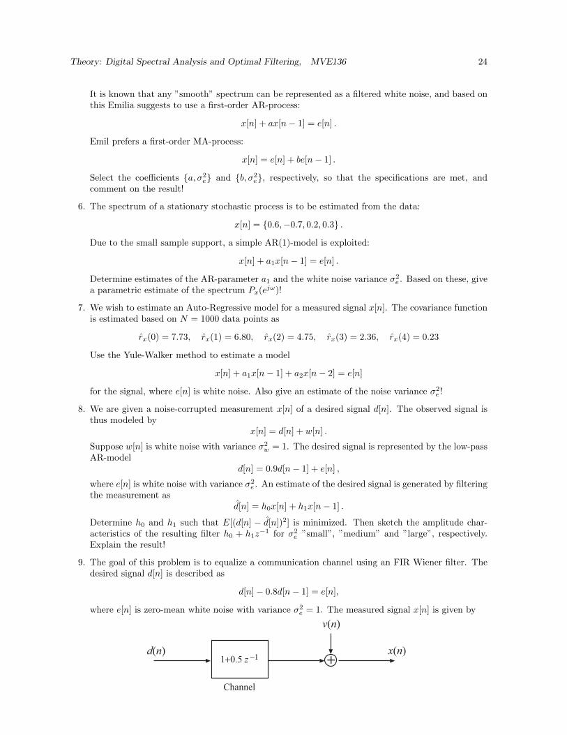
9. The goal of this problem is to equalize a communication channel using an FIR Wiener filter. Thedesired signal d[n] is described as

d[n]− 0.8d[n− 1] = e[n],

where e[n] is zero-mean white noise with variance σ2e = 1. The measured signal x[n] is given by

v(n)

x(n)d(n)+

−11+0.5 z

Channel


where v[n] is a zero-mean white noise with variance σ2v = 0.1. Determine a filter

d[n] = w0 x[n] + w1 x[n− 1]

so that E

[(d[n]− d[n]

)2]

is minimized!

10. A 2:nd order digital FIR notch filter can be designed by placing the zeros at e±jω. The resultingtransfer function is

H(z) = 1− 2 cosωz−1 + z−2.

Thus, a natural approach for estimating the frequency of a sine-wave is to apply a constrained FIRfilter

W (z) = 1− wz−1 + z−2

to the measured signal, and select w such that the output power is minimized. The frequency couldthen be estimated as ω = arccos w2 , provided |w| < 2. Now, suppose the measured signal is

x[n] = A cos(ω0n+ ϕ) + v[n],

where ϕ is a U(0, 2π) random phase and v[n] is a zero-mean stationary white noise. The filteroutput is given by

y[n] = x[n]− wx[n− 1] + x[n− 2] .

Find the w that minimizes E[y2[n]], and compute ω = arccos w2 . Then, prove that ω = ω0 forσ2v = 0, but that the estimate is otherwise biased.

7 Solutions to Selected Problems

1. In the method of periodogram averaging (Bartlett’s method), the available N samples are split intoK = N/M non-overlapping blocks, each of length M samples. The periodogram for each sub-blockis computed, and the final estimate is the average of these. The variance of each sub-periodogramis

V arP (i)per(e

jω) ≈ P 2x (ejω)

Thus, the normalized variance is

V arP (i)per(ejω)

P 2x (ejω)

≈ 1

or 100%. Assuming the sub-periodograms to be uncorrelated, averaging reduces the normalizedvariance to

V arPB(ejω)P 2x (ejω)

≈ 1/K

To achieve a normalized variance of 0.01 (1%) thus requires averaging K ≥ 100 sub-periodograms.Each sub-periodogram has the approximate frequency resolution ∆ω ≈ 2π/M , or ∆f ≈ 1/M . Inun-normalized frequency this becomes ∆F ≈ Fs/M Hz. With Fs = 1000 and a desired frequencyresolution of ∆F ≤ 1 Hz, the length of each sub-block must be M ≥ 1000. Together with K ≥ 100,this shows that the number of available samples must be N = KM ≥ 105. At 1 kHz, the datacollection takes at least 100 seconds.

3. For Blackman-Tukey’s method, the normalized variance is given by

ν =V arPBT (ejω)

P 2x (ejω)

≈ 1

N

M∑k=−M

w2lag[k] ,

where wlag[k] is the lag window. In this case we get

M∑k=−M

w2lag[k] =

100∑k=−100

e−0.2|k| = 2

100∑k=0

e−0.2k − 1 = 21− e−200

1− e−0.2− 1 ≈ 10 .

Thus, the normalized variance is ν = 10/N = 10−3.


4. The first model is an AR(2)-process:

x[n] + 0.6x[n− 1]− 0.2x[n− 2] = e[n]

Multiplying by x[n− k], k ≥ 0, and taking expectation leads to the relation

rx[k] + 0.6rx[k − 1]− 0.2rx[k − 2] = σ2e δ[k]

(Yule-Walker). With k = 0, 1, 2, we get three equations in three unknowns (see also the theorycomplement): 1 0.6 −0.2

0.6 1− 0.2 0−0.2 0.6 1

rx[0]rx[1]rx[2]

=

100

Solving this, for example using Matlab, leads to rx[0] = 2.4, rx[1] = −1.8 and rx[2] = 1.6. We canthen continue for k = 3, 4, . . . to get the autocorrelation at any lag, for example,

rx[3] = −0.6rx[2] + 0.2rx[1] = −1.3 , rx[4] = −0.6rx[3] + 0.2rx[2] = 1.1 .

It is of course also possible to solve the homogenous difference equation

rx[k] + 0.6rx[k − 1]− 0.2rx[k − 2] = 0 ,

with the given ”initial conditions”, to give the general solution. The spectrum of the AR model isgiven by

Px(ejω) =σ2e

|A(ejω)|2=

1

(1 + 0.6e−jω − 0.2e−j2ω)(1 + 0.6ejω − 0.2ej2ω)=

1

1.4 + 0.96 cosω − 0.4 cos 2ω

The second model is an MA(2) process:

x[n] = e[n] + 0.8e[n− 1] + 0.2e[n− 2]

In this case, the autocorrelation function is finite. First, multiply by x[n] and take expectation,which leads to

rx[0] = E(e[n] + 0.8e[n− 1] + 0.2e[n− 2])2 = (1 + 0.82 + 0.22)σ2e = 1.68 .

Next, multiply by x[n− 1] and take expectation:

rx[1] = E(e[n]+0.8e[n−1]+0.2e[n−2])(e[n−1]+0.8e[n−2]+0.2e[n−3]) = (0.8+0.2×0.8)σ2e = 0.96 .

Finally, multiplying by x[n− 2] and taking expectation leads to

rx[2] = E(e[n] + 0.8e[n− 1] + 0.2e[n− 2])(e[n− 2] + 0.8e[n− 3] + 0.2e[n− 4]) = 0.2 .

Multiplying by x[n − k], k > 2 and taking expectation wee see that rx[k] = 0, |k| > 2. Thespectrum of the MA process is given by

Px(ejω) = σ2e |B(ejω)|2 = (1+0.8e−jω+0.2e−j2ω)(1+0.8ejω+0.2ej2ω) = 1.68+1.92 cosω+0.4 cos 2ω

The third model is the ARMA(1,1) process:

x[n] + 0.8x[n− 1] = e[n]− 0.2e[n− 1]

In general, computing the autocorrelation function for an ARMA model is quite difficult. However,in the ARMA(1,1) case the following procedure is easiest. First, multiply by x[n − 1] and takeexpectation, which gives:

rx[1] + 0.8rx[0] = −0.2σ2e .


Second, square the ARMA model equation and again take expectation:

E(x[n] + 0.8x[n− 1])2 = E(e[n]− 0.2e[n− 1])2 .

This leads to1.64rx[0] + 1.6rx[1] = 1.04σ2

e .

Now we have two equations in the two unknowns rx[0] and rx[1]:[0.8 11.64 1.6

] [rx[0]rx[1]

]=

[−0.21.04

]Applying the usual formula for inverting a 2× 2 matrix, the solution is easily obtained as[

rx[0]rx[1]

]=

1

0.8× 1.6− 1× 1.64

[1.6 −1−1.64 0.8

] [−0.21.04

]≈[

3.8−3.2

].

The remaining auto-correlation parameters can be obtained by multiplying the ARMA equation byx[n− k], k ≥ 2 and taking expectation:

rx[k] + 0.8rx[k − 1] = 0 , k ≥ 2.

Thus, rx[2] = −0.8rx[1] ≈ 2.6 etc. In general, rx[k] = (−0.8)k−1rx[1] = (−0.8)k−1(−3.2) for k ≥ 2.The spectrum of the ARMA model is given by

Px(ejω) = σ2e

|B(ejω)|2

|A(ejω)|2=

(1− 0.2ejω)(1− 0.2e−jω)

(1 + 0.8ejω)(1 + 0.8e−jω)=

1− 0.4 cosω

1 + 1.6 cosω

5. For Emilia’s AR(1) model, the spectrum is given by

Px(ejω) =σ2e

(1− aejω)(1− ae−jω)=

σ2e

1 + a2 − 2a cosω

DC-level 1 means Px(ej0) = 1, which gives σ2e = 1 + a2 − 2a = (1− a)2. Cutoff frequency ωc = π/3

means Px(ejπ/3) = 1/2, and since cosπ/3 = 1/2 we get

(1− a)2

1 + a2 − a= 0.5

The solutions are a = (3 ±√

5)/2, from which we choose the stable solution (pole inside the unitcircle): a = (3−

√5)/2 ≈ 0.382, and σ2

e ≈ 0.382.

Emil’s MA(1) model givesPx(ejω) = σ2

e(1 + b2 + 2b cosω)

Thus we get σ2e = (1 + b)−2 and

1 + b2 + b

(1 + b)2= 0.5

This leads to b2 + 1 = 0, which does not have any real-valued solutions. The conclusion is that anMA(1) model cannot meet the specifications. In general, AR-models can be made ”sharper” thanMA-models for a given order. An MA-model is of course also possible in this case, but it requiresa higher order (how high?).

6. The Yule-Walker method gives the estimate

a1 = −rx[0]−1rx[1] .

With the given data, the sample autocorrelation function is calculated as

rx[0] =1

4(0.62 + 0.72 + 0.22 + 0.32) = 0.245


and

rx[1] =1

4(0.6× (−0.7) + (−0.7)× 0.2 + 0.2× 0.3) = −0.125

Thus, we get

a1 =0.125

0.245≈ 0.51 .

The noise variance estimate follows as

σ2e = rx[0] + a1rx[1] ≈ 0.18 .

8. The optimal filter (in the LMMSE sense) is given by the Wiener-Hopf (W-H) equations:∑k

h[k]rx[l − k] = rdx[l] .

In this case, the filter is a causal FIR filter with two taps (first-order filter):

d[n] = h0x[n] + h1x[n− 1] .

Thus, the W-H equations are

1∑k=0

hkrx[l − k] = rdx[l] , l = 0, 1.

In matrix form, this becomes [rx[0] rx[1]rx[1] rx[0]

] [h0

h1

]=

[rdx[0]rdx[1]

]The measured signal is given by

x[n] = d[n] + w[n] .

The auto-correlation function is then given by

rx[k] = E(d[n] + w[n])(d[n− k] + w[n− k]) = rd[k] + rw[k]

(since d[n] and w[n] are uncorrelated). Now, w[n] is white noise, so rw[k] = σ2wδ[k] = δ[k]. The

desired signal is the AR(1) process:

d[n]− 0.9d[n− 1] = e[n] .

To compute the autocorrelation function we use the Yule-Walker equations, which on matrix formbecome [

1 −0.9−0.9 1

] [rd[0]rd[1]

]=

[10

]σ2e .

Solving this gives [rd[0]rd[1]

]≈[

5.264.74

]σ2e .

Inserting the autocorrelation functions into the W-H equations now gives([5.26 4.744.74 5.26

]σ2e +

[1 00 1

])[h0

h1

]=

[5.264.74

]σ2e ,

where we have also used that rdx[k] = rd[k], since d[n] and w[n] are uncorrelated. It is possible, buta bit cumbersome, to solve this 2 × 2 system for a general σ2

e . Instead we take the extreme casesσ2e → 0 and σ2

e →∞ first, and then the intermediate case σ2e = 1. For σ2

e very small we have[h0

h1

]→[

5.264.74

]σ2e →

[00

].


Thus, when the SNR is very low, the estimation is d[n] = 0. For very large σ2e we have instead[

5.26 4.744.74 5.26

] [h0

h1

]=

[5.264.74

],

which gives the optimal FIR coefficients as[h0

h1

]=

[10

]Thus, in the high SNR case we take d[n] = x[n], i.e. no filtering is necessary. For the intermediatecase σ2

e = 1 we get [6.26 4.744.74 6.26

] [h0

h1

]=

[5.264.74

],

which leads to [h0

h1

]=

[0.630.28

].

The estimate is then d[n] = 0.62x[n] + 0.28x[n− 1], corresponding to the transfer function

H(ejω) = 0.62 + 0.28e−jω .

This is a low-pass filter with DC gain H(ej0) = 0.62 + 0.28 = 0.9, and 3 dB cutoff frequencyfc ≈ 0.25 ”per samples”. The filter is an optimal compromise for removing as much noise (whichhas a flat spectrum) as possible, without distorting the signal (which is low-pass) too much.

References

[1] S. L. Miller and D. G. Childers, Probability and Random Processes With Applications to Signal Pro-cessing and Communications. Elsevier Academic Press, Burlington, MA, 2004.

[2] A. V. Oppenheim, A. S. Willsky, and H. Nawab, Signals and Systems, 2nd ed. Prentice-Hall, UpperSaddly River, NJ, 1997.

[3] M. Hayes, Statistical Digital Signal Processing. John Wiley & Sons, New York, 1996.

[4] P. Stoica and R. Moses, Spectral Analysis of Signals. Prentice Hall, Upper Saddle River, NJ, 2005.

Complement on Digital Spectral Analysis and Optimal Filtering

Documents

Transcript of Complement on Digital Spectral Analysis and Optimal Filtering