Compile-Time Query Optimization for Big Data Analytics · collections that contain nested...
27
c 2019 by the authors; licensee RonPub, L ¨ ubeck, Germany. This article is an open access article distributed under the terms and conditions of the Creative Commons Attribution license (http://creativecommons.org/licenses/by/4.0/). Open Access Open Journal of Big Data (OJBD) Volume 5, Issue 1, 2019 http://www.ronpub.com/ojbd ISSN 2365-029X Compile-Time Query Optimization for Big Data Analytics Leonidas Fegaras University of Texas at Arlington, CSE, 416 Yates Street, P.O. Box 19015, Arlington, TX 76019, USA, [email protected] ABSTRACT Many emerging programming environments for large-scale data analysis, such as Map-Reduce, Spark, and Flink, provide Scala-based APIs that consist of powerful higher-order operations that ease the development of complex data analysis applications. However, despite the simplicity of these APIs, many programmers prefer to use declarative languages, such as Hive and Spark SQL, to code their distributed applications. Unfortunately, most current data analysis query languages are based on the relational model and cannot effectively capture the rich data types and computations required for complex data analysis applications. Furthermore, these query languages are not well-integrated with the host programming language, as they are based on an incompatible data model. To address these shortcomings, we introduce a new query language for data-intensive scalable computing that is deeply embedded in Scala, called DIQL, and a query optimization framework that optimizes and translates DIQL queries to byte code at compile-time. In contrast to other query languages, our query embedding eliminates impedance mismatch as any Scala code can be seamlessly mixed with SQL-like syntax, without having to add any special declaration. DIQL supports nested collections and hierarchical data and allows query nesting at any place in a query. With DIQL, programmers can express complex data analysis tasks, such as PageRank and matrix factorization, using SQL-like syntax exclusively. The DIQL query optimizer uses algebraic transformations to derive all possible joins in a query, including those hidden across deeply nested queries, thus unnesting nested queries of any form and any number of nesting levels. The optimizer also uses general transformations to push down predicates before joins and to prune unneeded data across operations. DIQL has been implemented on three Big Data platforms, Apache Spark, Apache Flink, and Twitter’s Cascading/Scalding, and has been shown to have competitive performance relative to Spark DataFrames and Spark SQL for some complex queries. This paper extends our previous work on embedded data-intensive query languages by describing the complete details of the formal framework and the query translation and optimization processes, and by providing more experimental results that give further evidence of the performance of our system. TYPE OF PAPER AND KEYWORDS Regular research paper: big data, distributed query processing, query optimization, embedded query languages 1 I NTRODUCTION In recent years, we have witnessed a growing interest in Data-Intensive Scalable Computing (DISC) programming environments for large-scale data analysis. One of the earliest and best known such environment is Map-Reduce, which was introduced by Google in 2004 [15] and later became popular as an open- source software with Apache Hadoop [5]. Map- 35
Transcript of Compile-Time Query Optimization for Big Data Analytics · collections that contain nested...
c© 2019 by the authors; licensee RonPub, Lubeck, Germany. This article is an open access article distributed under the terms and conditions ofthe Creative Commons Attribution license (http://creativecommons.org/licenses/by/4.0/).
Open Access
Open Journal of Big Data (OJBD)Volume 5, Issue 1, 2019
http://www.ronpub.com/ojbdISSN 2365-029X
Compile-Time Query Optimizationfor Big Data Analytics
Leonidas Fegaras
University of Texas at Arlington, CSE, 416 Yates Street, P.O. Box 19015, Arlington, TX 76019, USA,[email protected]
ABSTRACT
Many emerging programming environments for large-scale data analysis, such as Map-Reduce, Spark, and Flink,provide Scala-based APIs that consist of powerful higher-order operations that ease the development of complexdata analysis applications. However, despite the simplicity of these APIs, many programmers prefer to usedeclarative languages, such as Hive and Spark SQL, to code their distributed applications. Unfortunately, mostcurrent data analysis query languages are based on the relational model and cannot effectively capture the richdata types and computations required for complex data analysis applications. Furthermore, these query languagesare not well-integrated with the host programming language, as they are based on an incompatible data model.To address these shortcomings, we introduce a new query language for data-intensive scalable computing thatis deeply embedded in Scala, called DIQL, and a query optimization framework that optimizes and translatesDIQL queries to byte code at compile-time. In contrast to other query languages, our query embedding eliminatesimpedance mismatch as any Scala code can be seamlessly mixed with SQL-like syntax, without having to add anyspecial declaration. DIQL supports nested collections and hierarchical data and allows query nesting at any placein a query. With DIQL, programmers can express complex data analysis tasks, such as PageRank and matrixfactorization, using SQL-like syntax exclusively. The DIQL query optimizer uses algebraic transformations toderive all possible joins in a query, including those hidden across deeply nested queries, thus unnesting nestedqueries of any form and any number of nesting levels. The optimizer also uses general transformations to pushdown predicates before joins and to prune unneeded data across operations. DIQL has been implemented on threeBig Data platforms, Apache Spark, Apache Flink, and Twitter’s Cascading/Scalding, and has been shown to havecompetitive performance relative to Spark DataFrames and Spark SQL for some complex queries. This paperextends our previous work on embedded data-intensive query languages by describing the complete details of theformal framework and the query translation and optimization processes, and by providing more experimental resultsthat give further evidence of the performance of our system.
TYPE OF PAPER AND KEYWORDS
Regular research paper: big data, distributed query processing, query optimization, embedded query languages
1 INTRODUCTION
In recent years, we have witnessed a growinginterest in Data-Intensive Scalable Computing (DISC)programming environments for large-scale data analysis.
One of the earliest and best known such environmentis Map-Reduce, which was introduced by Google in2004 [15] and later became popular as an open-source software with Apache Hadoop [5]. Map-
35
Open Journal of Big Data (OJBD), Volume 5, Issue 1, 2019
reduce is a simple and powerful interface that enablesautomatic parallelization and distribution of large-scalecomputations on large clusters of commodity (low-end)processors [15]. However, because of its simplicity,it soon became apparent that the Map-Reduce modelhas many limitations and drawbacks that impose a highoverhead to complex workflows and graph algorithms.One of its major drawbacks is that, to simplify reliabilityand fault tolerance, the Map-Reduce engine stores theintermediate results between the map and reduce stagesand between consecutive Map-Reduce jobs on secondarystorage, rather than in memory. To address some of theshortcomings of the Map-Reduce model, new alternativeframeworks have been introduced recently. Amongthem, the most promising frameworks that seem to begood alternatives to Map-Reduce while addressing itsdrawbacks are Apache Spark [7] and Apache Flink [4],which cache most of their data in the memory of theworker nodes.
The Map-Reduce framework was highly inspiredby the functional programming style by requiring twofunctions to express a Map-Reduce job: the map functionspecifies how to process a single key-value pair togenerate a set of intermediate key-value pairs, while thereduce function specifies how to combine and aggregateall intermediate values associated with the sameintermediate key to compute the resulting key-valuepairs. Similarly, Spark and Flink provide a functionalprogramming API to process distributed data collectionsthat resembles the way modern functional programminglanguages operate on regular data collections, such aslists and arrays, using higher-order operations, suchas map, filter, and reduce. By adopting a functionalprogramming style, not only do these frameworksprevent interference among parallel tasks, but theyalso facilitate a functional style in composing complexdata analysis computations using powerful higher-orderoperations as building blocks.
Furthermore, many of these frameworks provide aScala-based API, because Scala is emerging as thefunctional language of choice for Big Data analytics.Examples of such APIs include the Scala-based APIs forHadoop Map-Reduce, Scalding [31] and Scrunch [32],and the Hadoop alternatives, Spark [7] and Flink [4].These APIs are based on distributed collections thatresemble regular Scala data collections as they supportsimilar methods. Although these distributed collectionscome under different names, such as TypedPipes inScalding, PCollections in Scrunch, RDDs in Spark,and DataSets in Flink, they all represent immutablehomogeneous collections of data distributed acrossthe compute nodes of a cluster and they are verysimilar. By providing an API that is similar to theScala collection API, programmers already familiar
with Scala programming can start developing distributedapplications with minimal training. Furthermore, manyBig Data analysis applications need to work on nestedcollections, because, unlike relational databases, theyneed to analyze data in their native format, as theybecome available, without having to normalize thesedata into flat relations first and then reconstruct thedata during querying using expensive joins. Thus,data analysis applications often work on distributedcollections that contain nested sub-collections. Whileouter collections need to be distributed to be processedin parallel, the inner sub-collections must be storedin memory and processed as regular Scala collections.By providing similar APIs for both distributed datasetsand in-memory collections, these frameworks providea uniform way for processing data collections thatsimplifies program development considerably.
Although DISC frameworks provide powerful APIsthat are simple to understand, it is hard to developnon-trivial applications coded in a general-purposeprogramming language, especially when the focusis in optimizing performance. Much of the timespent programming these APIs is for addressing theintricacies and avoiding the pitfalls inherent to theseframeworks. For instance, if the functional argumentof a Spark operation accesses a non-local variable,the value of this variable is implicitly serialized andbroadcast to all the worker nodes that evaluate thisfunction. This broadcasting is completely hidden fromthe programmers, who must now make sure that there isno accidental reference to a large data structure withinthe functional parameters. Furthermore, the implicitbroadcasting of non-local variables is less efficient thanthe explicit peer-to-peer broadcast operation in Spark,which uses faster serialization formats.
A common error made by novice Spark programmersis to try to operate on an RDD from within the functionalargument of another RDD operation, only to discoverat run-time that this is impossible since functionalarguments are evaluated by each worker node whileRDDs must be distributed across the worker nodes.Instead, programmers should either broadcast the innerRDD to the worker nodes before the outer operation oruse a join to combine the two RDDs. More importantly,some optimizations in the core Spark API, such ascolumn pruning and selection pushdown, must be doneby hand, which is very hard and may result to obscurecode that does not reflect the intended applicationlogic. Very often, one may have to choose amongalternative operations that have the same functionalitybut different performance characteristics, such as usinga reduceByKey operation instead of a groupByKeyfollowed by a reduce operation. Furthermore, the coreSpark API does not provide alternative join algorithms,
36
L. Fegaras: Compile-Time Query Optimization for Big Data Analytics
such as broadcast and sort-merge joins, thus leaving thedevelopment of these algorithms to the programmers,which duplicates efforts and may lead to suboptimalperformance.
In addition to hand-optimizing programs expressedin these APIs, there are many configuration parametersto adjust for better performance that overwhelm non-expert users. To find an optimal configuration for acertain data analysis application in Spark, one mustdecide how many executors to use, how many coresand how much memory to allocate per executor, howmany partitions to split the data, etc. Furthermore, toimprove performance, one can specify the number ofreducers in Spark operations that cause data shuffling,instead of using the default, or even repartition the datain some cases to modify the degree of parallelism or toreduce data skew. Such adjustments are unrelated to theapplication logic but affect performance considerably.
Because of the complexity involved in developing andfine-tuning data analysis applications using the providedAPIs, most programmers prefer to use declarativedomain-specific languages (DSLs), such as Hive [6],Pig [30], MRQL [18], and Spark SQL [8], to codetheir distributed applications, instead of coding themdirectly in an algorithmic language. Most of these DSL-based frameworks though provide a limited syntax foroperating on data collections, in the form of simple joinsand group-bys. Some of them have limited supportfor nested collections and hierarchical data, and cannotexpress complex data analysis tasks, such as PageRankand data clustering, using DSL syntax exclusively. SparkDataFrames, for example, allows nested collections butprovides a naıve way to process them: one must usethe ‘explode’ operation on a nested collection in a rowto flatten the row to multiple rows. Hive supports‘lateral views’ to avoid creating intermediate tables whenexploding nested collections. Both Hive and DataFramestreat in-memory collections differently from distributedcollections, resulting to an awkward way to query nestedcollections.
One of the advantages of using DSL-based systemsin developing DISC applications is that these systemssupport automatic program optimization. Such programoptimization is harder to achieve in an API-basedsystem. Some API-based systems though have foundways to circumvent this shortcoming. The evaluation ofRDD transformations in Spark, for example, is deferreduntil an action is encountered that brings data to themaster node or stores the data into a file. Spark collectsthe deferred transformations into a DAG and dividesthem into subsequences, called stages, which are similarto Pig’s Map-Reduce barriers. Data shuffling occursbetween stages, while transformations within a stage arecombined into a single RDD transformation. Unlike Pig
though, Spark cannot perform non-trivial optimizations,such as moving a filter operation before a join, becausethe functional arguments of the RDD operations arewritten in the host language and cannot be analyzedfor code patterns at run-time. Spark has addressed thisshortcoming by providing two additional APIs, calledDataFrames and Datasets [34].
A Dataset combines the benefits of RDD (strongtyping and powerful higher-order operations) with SparkSQL’s optimized execution engine. A DataFrame is aDataset organized into named columns as in a relationaltable. SQL queries in DataFrames are translated andoptimized to RDD workflows at run-time using theCatalyst architecture. The optimizations include pushingdown predicates, column pruning, and constant folding,but there are also plans for providing cost-based queryoptimizations, such as join reordering. Spark SQLthough cannot handle most forms of nested queries anddoes not support iteration, thus making it inappropriatefor complex data analysis applications. One commoncharacteristic of most DSL-based frameworks is that,after optimizing a DSL program, they compile it tomachine code at run-time, using an optimizing codegenerator, such as LLVM, or run-time reflection in Javaor Scala.
Our goal is to design a query language for DISCapplications that can be fully and effectively embeddedinto a host programming language (PL). To minimizeimpedance mismatch, the query data model must beequivalent to that of the PL. This restriction alonemakes relational query languages a poor choice forquery embedding since they cannot embed nestedcollections from the host PL into a query. Furthermore,data-centric query languages must work on specialcollections, which may have different semantics fromthe collections provided by the host PL. For instance,DISC collections are distributed across the worker nodes.To minimize impedance mismatch, data-centric andPL collections must be indistinguishable in the querylanguage, although they may be processed differently bythe query system.
In addition, the presence of null values complicatesquery embedding because, unlike SQL, which uses 3-valued logic to handle null markers introduced by outerjoins, most PLs do not provide a standardized way totreat nulls. Instead, one would have to write explicitcode in the query to handle them. Thus, embedding PL-defined UDF calls and custom aggregations in a querycan either be done by writing explicit code in the queryto handle nulls before these calls or by avoiding nullvalues in the query data model altogether. We adopt thelatter approach because we believe that nulls complicatequery semantics and query embedding, and may resultto obscure queries. Banning null values though means
37

Open Journal of Big Data (OJBD), Volume 5, Issue 1, 2019
banning outer joins, which are considered importantfor practical query languages. In SQL, for example,matrix addition of sparse matrices can be expressed asa full outer join, to handle the missing entries in sparsematrices.
In a data model that supports nested collectionsthough, outer joins can be effectively captured by acoGroup operation (as defined in Pig, Spark, and manyother DISC frameworks), which does not introduceany nulls. This implies that we can avoid generatingnull values as long as we provide syntax in thequery language that captures any coGroup operation.Furthermore, most outer semijoins, which are verycommon in complex data-centric applications, can bemore naturally expressed as nested queries. Thus,a query language must allow any arbitrary form ofquery nesting, while the query processor must beable to evaluate nested queries efficiently using joins.Consequently, query unnesting (i.e., finding all possiblejoins across nested queries) is crucial for embeddedquery languages. Current DISC query languages havevery limited support for query nesting. Hive and SparkSQL, for example, support very simple forms of querynesting in predicates, thus forcing the programmers touse explicit outer joins to simulate the other forms ofnested queries and write code to handle nulls.
We present a new query language for DISC systemsthat is deeply embedded in Scala, called DIQL [20], anda query optimization framework that optimizes DIQLqueries and translates them to Java byte code at compile-time. DIQL is designed to support multiple Scala-based APIs for distributed processing by abstractingtheir distributed data collections as a DataBag, whichis a bag distributed across the worker nodes of acomputer cluster. Currently, DIQL supports threeBig Data platforms that provide different APIs andperformance characteristics: Apache Spark, ApacheFlink, and Twitter’s Cascading/Scalding. Unlike otherquery languages for DISC systems, DIQL can uniformlywork on both distributed and in-memory collectionsusing the same syntax. DIQL allows seamless mixing ofnative Scala code, which may contain UDF calls, withSQL-like query syntax, thus combining the flexibilityof general-purpose programming languages with thedeclarativeness of database query languages.
DIQL queries may use any Scala pattern, may accessany Scala variable, and may embed any Scala codewithout any marshaling. More importantly, DIQLqueries can use the core Scala libraries and tools aswell as user-defined classes without having to addany special declaration. This tight integration withScala eliminates impedance mismatch, reduces programdevelopment time, and increases productivity, since itfinds syntax and type errors at compile-time. DIQL
supports nested collections and hierarchical data, andallows query nesting at any place in a query. The queryoptimizer can find any possible join, including joinshidden across deeply nested queries, thus unnesting anyform of query nesting. The DIQL algebra, which isbased on monoid homomorphisms, can capture all thelanguage features using a very small set of homomorphicoperations. Monoids and monoid homomorphisms fullycapture the functionality provided by current DSLs forDISC processing by directly supporting operations, suchas group-by, order-by, aggregation, and joins on complexcollections.
The intended users of DIQL are developers of DISCapplications who 1) have a preference in declarativequery languages, such as SQL, over the higher-orderfunctional programming style used by DISC APIs, 2)want to use a full fledged query language that istightly integrated with the host language, combining theflexibility of general-purpose programming languageswith the declarativeness of database query languages,3) want to express their applications in a platform-independent language and experiment with multipleDISC platforms without modifying their programs, 4)want to focus on the programming logic without havingto add obscure and platform-dependent performancedetails to the code, and 5) want to achieve goodperformance by relying on a sophisticated queryoptimizer.
The contributions of this paper can be summarized asfollows:
• We introduce a novel query language for large-scaledistributed data analysis that is deeply embedded inScala, called DIQL (Section 3). Unlike other DISCquery languages, the query checking and codegeneration are done at compile-time. With DIQL,programmers can express complex data analysistasks, such as PageRank, k-means clustering,and matrix factorization, using SQL-like syntaxexclusively.
• We present an algebra for DISC, called the monoidalgebra, which captures most features supported bycurrent DISC frameworks (Section 4), and rulesfor translating DIQL queries to the monoid algebra(Section 5).
• We present algebraic transformations for derivingjoins from nested queries that unnest nested queriesof any form and any number of nesting levels,for pushing down predicates before joins, and forpruning unneeded data across operations, whichgeneralize existing techniques (Section 6).
• We report on a prototype implementation of DIQLon three Big Data platforms, Spark, Flink, and
38
L. Fegaras: Compile-Time Query Optimization for Big Data Analytics
Scalding (Section 7) and explain how the DIQLtype inference system is integrated with the Scalatyping system using Scala’s compile-time reflectionfacilities and macros.
• We give evidence that DIQL has competitiveperformance relative to Spark DataFrames andSpark SQL by evaluating a simple nested query, ak-means clustering query, and a PageRank query(Section 9).
The DIQL syntax and some of the performance resultshave been presented in an earlier work [20]. The workreported in this paper extends our earlier work in fourways: 1) it fully describes the monoid algebra, whichis used as the formal basis for our framework and as thetarget of query translation, 2) it gives the complete detailsof translating the DIQL syntax to algebraic terms, 3) itfully describes the query optimization framework, and4) it provides more experimental results that give furtherevidence that our system has competitive performancerelative to Spark DataFrames and Spark SQL.
2 RELATED WORK
One of the earliest DISC frameworks was the Map-Reduce model, which was introduced by Googlein 2004 [15]. The most popular Map-Reduceimplementation is Apache Hadoop [5], an open-sourceproject developed by Apache, which is used today bymany companies to perform data analysis. RecentDISC systems go beyond Map-Reduce by maintainingdataset partitions in the memory of the worker nodes.Examples of such systems include Apache Spark [7] andApache Flink [4]. There are also a number of higher-level languages that make Map-Reduce programmingeasier, such as HiveQL [36], PigLatin [30], SCOPE [13],DryadLINQ [37], and MRQL [18].
Apache Hive [36] provides a logical RDBMSenvironment on top of the Map-Reduce engine, well-suited for data warehousing. Using its high-level querylanguage, HiveQL, users can write declarative queries,which are optimized and translated into Map-Reducejobs that are executed using Hadoop. HiveQL does nothandle nested collections uniformly: it uses SQL-likesyntax for querying data sets but uses vector indexingfor nested collections. Apache Pig [21] provides a user-friendly scripting language, called PigLatin [30], on topof Map-Reduce, which allows explicit filtering, map,join, and group-by operations. Programs in PigLatinare written as a sequence of steps (a dataflow), whereeach step carries out a single data transformation. Thissequence of steps is not necessarily executed in thatorder; instead, when a store operation is encountered,
Pig optimizes the dataflow into a number of Map-Reducebarriers, which are executed as Map-Reduce jobs. Eventhough the PigLatin data model is nested, its languageis less declarative than DIQL and does not supportquery nesting, but can simulate it using outer joins andcoGroup.
In addition to the DSLs for data-intensiveprogramming, there are some Scala-based APIsthat simplify Map-Reduce programming, such as,Scalding [31], which is part of Twitter’s Cascading [12],Scrunch [32], which is a Scala wrapper for the ApacheCrunch, and Scoobi. These APIs support higher-order operations, such as map and filter, which arevery similar to those for Spark and Flink. Slick [33]integrates databases directly into Scala, allowingstored and remote data to be queried and processedin the same way as in-memory data, using ordinaryScala classes and collections. Summingbird [11] is anAPI-based distributed system that supports run-timeoptimization and can run on both Map-Reduce andStorm. Compared to Spark and Flink, the SummingbirdAPI is intentionally more restrictive to facilitateoptimization at run-time. The main shortcoming of allthese API-based approaches is their inability to analyzethe functional arguments of their high-level operationsat run-time to do complex optimizations.
Vertex-centric graph-parallel programming is a newpopular framework for large-scale graph processing. Itwas introduced by Google’s Pregel [28] but is nowavailable by many open-source projects, such as ApacheGiraph and Spark’s GraphX. Most of these frameworksare based on the Bulk Synchronous Parallelism (BSP)programming model. VERTEXICA [26] and Grail [16]provide the same vertex-centric interface as Pregel but,instead of a distributed file system, they use a relationaldatabase to store the graph and the exchanged messagesacross the BSP supersteps. Unlike Grail, which can runon a single server only, VERTEXICA can run on multipleparallel machines connected to the same database server.Such configuration may not scale out very well becausethe centralized database may become the bottleneck ofall the data traffic across the machines. Although DIQLis a general-purpose DISC query system, graph queriesin DIQL are expressed using SQL-like syntax sincegraphs are captured as regular distributed collections.These queries are translated to distributed self-joins overthe graph data. In [17], we proved that the monoidalgebra can simulate any BSP computation (includingvertex-centric parallel programs) efficiently, requiringthe same amount of data shuffling as a typical BSPimplementation.
DryadLINQ [37] is a programming model for largescale data-parallel computing that translates programsexpressed in the LINQ programming model to Dryad,
39
Open Journal of Big Data (OJBD), Volume 5, Issue 1, 2019
which is a distributed execution engine for data-parallelapplications. Like DIQL, LINQ is a statically stronglytyped language and supports a declarative SQL-likesyntax. Unlike DIQL, though, the LINQ query syntax isvery limited and has limited support for query nesting.DryadLINQ allows programmers to provide manualhints to guide optimization. Currently, it performs staticoptimizations based on greedy heuristics only, but thereare plans to implement cost-based optimizations in thefuture.
Apache Calcite [9] is a widely adopted relationalquery optimizer with a focus on flexibility, adaptivity,and extensibility. It is used for query optimization bya large number of open-source data-centric frameworks,including many DISC systems, such as Hive, Spark,Storm, and Flink. Although it can be adapted to workwith many different platforms, its data model is purelyrelational with very little support for nested collections(it only supports indexing on inner collections), while itsalgebra is purely relational with no support for nestedqueries, such as, a query in a filter predicate.
There are some recent proposals for speeding up queryplan interpretation in Volcano-style iterator-based queryprocessing engines, used by many relational databasesystems, especially for main memory database systemsfor which CPU cost is important. Some of these systemsare using a compiled execution engine to avoid theinterpretation cost of algebraic expressions in a queryplan. The HyPer database system [29], for example,translates algebraic expressions in a query to low-levelLLVM code on the fly, so that the plan iterators areevaluated in a push-based fashion using loops. Insteadof generating low-level code at once during the earlystages of compilation, LegoBase [27] produces low-levelC code in stages. It uses generative metaprogrammingin Scala to take advantage of the type system of thelanguage to check the correctness of the generatedcode, and to allow optimization and recompilation ofcode at various execution stages, including at run-time. Compared to our work, which also generatestype-correct code at compile time, their focus is in therelational model and SQL, while ours is in a nested datamodel and complex nested queries, and their target isrelational engines, while ours is DISC APIs.
Our work on embedded DSLs has been inspiredby Emma [2, 3]. Unlike our work, Emma does notprovide an SQL-like query syntax; instead, it usesScala’s for-comprehensions to query datasets. These for-comprehensions are optimized and translated to abstractdataflows at compile-time, and these dataflows areevaluated at run-time using just-in-time code generation.Using the host language syntax for querying allowsa deeper embedding of DSL code into the hostlanguage but it requires that the host language supports
meta-programming and provides a declarative syntaxfor querying collections, such as for-comprehensions.Furthermore, Scala’s for-comprehensions do not providea declarative syntax for group-by. Emma’s core primitivefor data processing is the fold operation over the union-representation of bags, which is equivalent to a baghomomorphism. The fold well-definedness conditionsare similar to the preconditions for bag homomorphisms.Scala’s for-comprehensions are translated to monadcomprehensions, which are desugared to monadoperations, which, in turn, are expressed in terms of fold.Other non-monadic operations, such as aggregations,are expressed as folds. Emma also provides additionaloperations, such as groupBy and join, but does notprovide algebraic operations for sorting, outer-join(needed for non-trivial query unnesting), and repetition(needed for iterative workflows). Unlike DIQL, Emmadoes not provide general methods to convert nestedcorrelated queries to joins, except for simple nestedqueries in which the domain of a generator qualifier isanother comprehension.
The syntax and semantics of DIQL have beeninfluenced by previous work on list comprehensions withorder-by and group-by [39]. Monoid homomorphismsand monoid comprehensions were first introduced asa formalism for OO queries in [19] and later as aquery algebra for MRQL [18]. Our monoid algebraextends these algebras to include group-by, coGroup,and order-by operations. Many other algebras andcalculi are based on monads and monad comprehensions.Monad comprehensions have a number of limitations,such as inability to capture grouping and sorting onbags. Monads also require various extensions to captureaggregations and heterogeneous operations, such as,converting a list to a bag. Monoids on the otherhand can naturally capture aggregations, ordering, andgroup-by without any extension. Many other algebrasand calculi in related work are based on monadcomprehensions [38]. In an earlier work [17], we haveshown that monoid comprehensions are a better formalbasis for practical DISC query languages than monadcomprehensions.
The syntax of DIQL is based on the syntax ofMRQL [18], which is a query language for large-scale,distributed data analysis. The design of MRQL, inturn, has been influenced by XQuery and ODMG OQL,although it uses SQL-like syntax. Unlike MRQL, DIQLallows general Scala patterns and expressions in a query,it is more tightly integrated with the host language, and itis optimized and compiled to byte code at compile-time,instead of run-time.
40
L. Fegaras: Compile-Time Query Optimization for Big Data Analytics
3 DIQL: A DATA-INTENSIVE QUERYLANGUAGE
This section presents the detailed syntax of DIQL.As an example of a DIQL query evaluated on Spark,consider matrix multiplication. We can represent asparse matrix M as a distributed collection of typeRDD[(Double,Int,Int)] in Spark, so that a triple (v, i, j)in this collection represents the matrix element v =Mij . Then the matrix multiplication between two sparsematrices X and Y can be expressed as follows in DIQL:
Query A:select (+/z, i, j)from (x, i, k) <− X, (y, k , j) <− Y, z = x ∗ ywhere k == kgroup by (i, j)
where X and Y are embedded Scala variables of typeRDD[(Double,Int,Int)]. This query retrieves the valuesXik ∈ X and Ykj ∈ Y for all i, j, k, and sets z = Xik ∗Ykj . The group-by operation lifts each pattern variabledefined before the group-by (except the group-by keys)from some type t to a bag of t, indicating that eachsuch variable must now contain all the values associatedwith the same group-by key value. Consequently, afterwe group the values by the matrix indexes i and j, thevariable z is lifted to a bag of numerical valuesXik∗Ykj ,for all k. Hence, the aggregation +/z will sum up all thevalues in the bag z, deriving
∑kXik ∗ Ykj for the ij
element of the resulting matrix.As another example, consider the matrix addition
between the two sparse matrices X and Y . Giventhat missing values in sparse matrices correspond tozero values, matrix addition should be expressed in arelational query as a full outer join, not an inner join.Instead, this operation is specified as follows in DIQL:
Query B:select (+/(x++y), i, j)from (x, i, j) <− X group by (i, j)from (y, i , j ) <− Y group by (i , j )
Each of the two group-by clauses in this query groupsonly the variables in their associated from-clause: Xvalues are grouped by (i, j) and Y values are grouped by(i , j ). Furthermore, the two group keys are implicitlyset to be equal, (i, j) = (i , j ). That is, after Xis grouped by (i, j) and Y is grouped by (i , j ), theresulting grouped datasets are joined over their group-by key. That is, this query is equivalent to a coGroupoperation found in many DISC APIs. The semantics ofthis double group-by query is very similar to that of thesingle group-by: The first (resp. second) group-by liftsthe variable x (resp. y) to a bag of Double, which may
be either empty or singleton. That is, the concatenationx++y may contain one or two values, which are addedtogether in +/(x++y). In contrast to a relational outerjoin, this query does not introduce any null values sinceit is equivalent to a coGroup operation.
Many emerging Scala-based APIs for distributedprocessing, such as the Scala-based Hadoop Map-Reduce frameworks Scalding and Scrunch, and theMap-Reduce alternatives Spark and Flink, are basedon distributed collections that resemble regular Scaladata collections as they support similar methods. ManyBig Data analysis applications need to work on nestedcollections, because, unlike relational databases, theyneed to analyze data in their native format, as theybecome available, without having to normalize these datainto flat relations first. While outer collections needto be distributed in order to be processed in parallel,the inner sub-collections must be stored in memory andprocessed as regular Scala collections. Processing bothkinds of collections, distributed and in-memory, usingthe same syntax or API simplifies program developmentconsiderably. The DIQL syntax treats distributedand in-memory collections in the same way, althoughDIQL optimizes and compiles the operations on thesecollections differently. The DIQL data model supportsfour collection types: a bag, which is an unorderedcollection (a multiset) of values stored in memory, aDataBag, which is a bag distributed across the workernodes of a computer cluster, a list, which is an orderedcollection of values stored in memory, and a DataList,which is an ordered DataBag.
For example, let R and S be two distributedcollections in Spark of type RDD[(Long,Long)] andRDD[(Long,Long,Long)], respectively. Then thefollowing Scala code fragment that contains a DIQLquery joins the datasets R and S using a nested query:
Query C:q(”””
select ( x, +/(select bfrom (a,b, ) <− S
where a==y) )from (x,y) <− R
”””)
In SQL, this query would have been written as a left-outer join between R and S, followed by a group-by withan aggregation. The DIQL syntax can be embedded in aScala program using the Scala macro q(” ” ” ... ” ” ” ), whichis optimized and compiled to byte code at compile-time. This byte code in turn is embedded in the bytecode generated by the rest of the Scala program. Thatis, all type errors in the DIQL queries are captured atcompile-time. Furthermore, a query can see any activeScala declaration in the current Scala scope, including
41
Open Journal of Big Data (OJBD), Volume 5, Issue 1, 2019
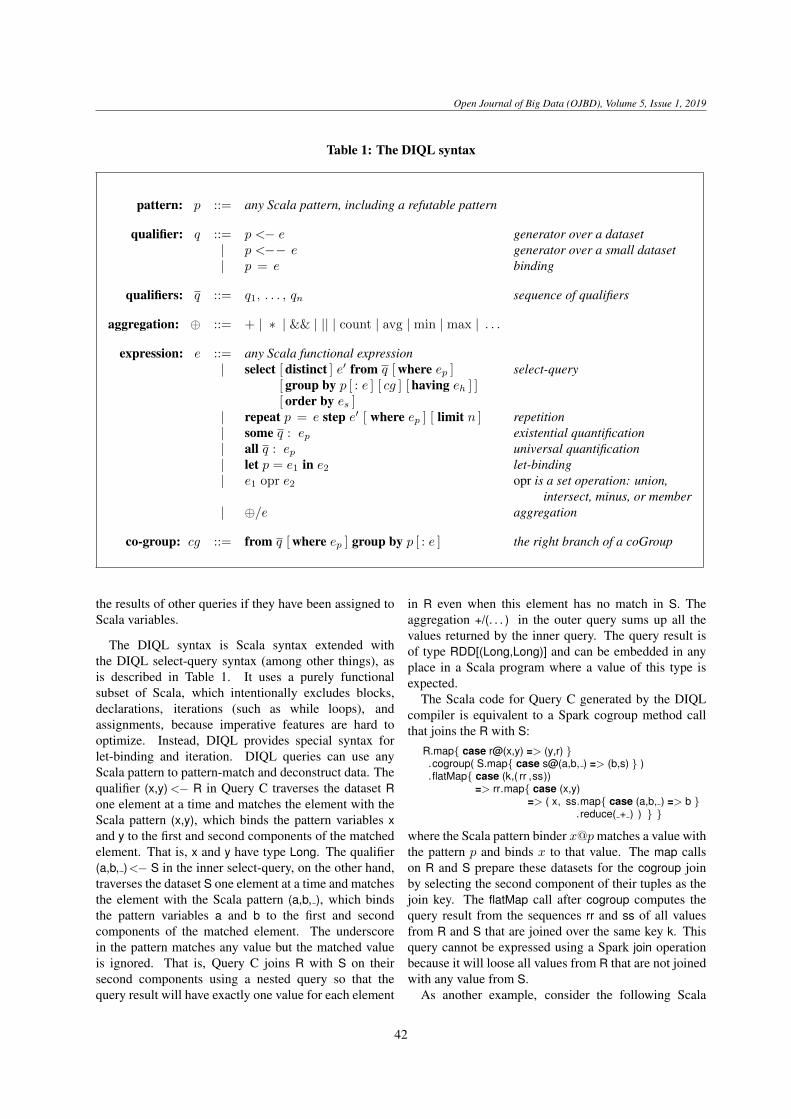
Table 1: The DIQL syntax
pattern: p ::= any Scala pattern, including a refutable pattern
qualifier: q ::= p <− e generator over a dataset| p <−− e generator over a small dataset| p = e binding
qualifiers: q ::= q1, . . . , qn sequence of qualifiers
aggregation: ⊕ ::= + | ∗ | && | || | count | avg | min | max | . . .
expression: e ::= any Scala functional expression| select [ distinct ] e′ from q [ where ep ] select-query
[ group by p [ : e ] [ cg ] [ having eh ] ][ order by es ]
| repeat p = e step e′ [ where ep ] [ limit n ] repetition| some q : ep existential quantification| all q : ep universal quantification| let p = e1 in e2 let-binding| e1 opr e2 opr is a set operation: union,
intersect, minus, or member| ⊕/e aggregation
co-group: cg ::= from q [ where ep ] group by p [ : e ] the right branch of a coGroup
the results of other queries if they have been assigned toScala variables.
The DIQL syntax is Scala syntax extended withthe DIQL select-query syntax (among other things), asis described in Table 1. It uses a purely functionalsubset of Scala, which intentionally excludes blocks,declarations, iterations (such as while loops), andassignments, because imperative features are hard tooptimize. Instead, DIQL provides special syntax forlet-binding and iteration. DIQL queries can use anyScala pattern to pattern-match and deconstruct data. Thequalifier (x,y)<− R in Query C traverses the dataset Rone element at a time and matches the element with theScala pattern (x,y), which binds the pattern variables xand y to the first and second components of the matchedelement. That is, x and y have type Long. The qualifier(a,b, )<− S in the inner select-query, on the other hand,traverses the dataset S one element at a time and matchesthe element with the Scala pattern (a,b, ), which bindsthe pattern variables a and b to the first and secondcomponents of the matched element. The underscorein the pattern matches any value but the matched valueis ignored. That is, Query C joins R with S on theirsecond components using a nested query so that thequery result will have exactly one value for each element
in R even when this element has no match in S. Theaggregation +/(. . . ) in the outer query sums up all thevalues returned by the inner query. The query result isof type RDD[(Long,Long)] and can be embedded in anyplace in a Scala program where a value of this type isexpected.
The Scala code for Query C generated by the DIQLcompiler is equivalent to a Spark cogroup method callthat joins the R with S:
R.map{ case r@(x,y) => (y,r) }.cogroup( S.map{ case s@(a,b, ) => (b,s) } ).flatMap{ case (k,( rr ,ss))
=> rr.map{ case (x,y)=> ( x, ss.map{ case (a,b, ) => b }
.reduce( + ) ) } }
where the Scala pattern binder x@pmatches a value withthe pattern p and binds x to that value. The map callson R and S prepare these datasets for the cogroup joinby selecting the second component of their tuples as thejoin key. The flatMap call after cogroup computes thequery result from the sequences rr and ss of all valuesfrom R and S that are joined over the same key k. Thisquery cannot be expressed using a Spark join operationbecause it will loose all values from R that are not joinedwith any value from S.
As another example, consider the following Scala
42
L. Fegaras: Compile-Time Query Optimization for Big Data Analytics
class that represents a graph node:
case class Node ( id: Long, adjacent: List [Long] )
where adjacent contains the ids of the node’s neighbors.Then, a graph in Spark can be represented as a distributedcollection of type RDD[Node]. Note that the innercollection of type List[Long] is an in-memory collectionsince it conforms to the class Traversable. The followingDIQL query constructs the graph RDD from a text filestored in HDFS and then transforms this graph so thateach node is linked with the neighbors of its neighbors:
Query D:let graph = select Node( id = n, adjacent = ns )
from line <− sc.textFile(”graph.txt ” ),n ::ns = line . split ( ” , ” ). toList
.map( .toLong)in select Node( x, ++/ys )
from Node(x,xs) <− graph,a <− xs,Node(y,ys) <− graph
where y == a group by x
In the previous DIQL query, the let-binding binds thenew variable graph to an RDD of type RDD[Node],which contains the graph nodes read from HDFS, mixingDIQL syntax with Spark API methods. The DIQL type-checker will infer that the type of sc.textFile(”graph.txt”)is RDD[String], and, hence, the type of the query variableline is String. Based on this information, the DIQL type-checker will infer that the type of n:ns in the patternof the let-binding is List[Long], which is a Traversablecollection. The select-query in the body of the let-binding expresses a self-join over graph followed by agroup-by. The pattern Node(x,xs) matches one graphelement at a time (a Node) and binds x to the node id andxs to the adjacent list of the node. Hence, the domain ofthe second qualifier a<− xs is an in-memory collectionof type List[Long], making ‘a’ a variable of type Long.The graph is traversed a second time and its elementsare matched with Node(y,ys). Thus, this select-querytraverses two distributed and one in-memory collections.
In general, as we can see in Table 1, a select-querymay have multiple qualifiers in the ‘from’ clause of thequery. A qualifier p<− e, where e is a DIQL expressionthat returns a data collection and p is a Scala pattern(which can be refutable - i.e., it may fail to match),iterates over the collection and, each time, the currentelement of the collection is pattern-matched with p,which, if the match succeeds, binds the pattern variablesin p to the matched components of the element. Thequalifier p<−− e does the same iteration as p<− e but italso gives a hint to the DIQL optimizer that the collectione is small (can fit in the memory of a worker node) so thatthe optimizer may consider using a broadcast join. Thebinding p = e pattern-matches the pattern p with the
value returned by e and, if the match succeeds, binds thepattern variables in p to the matched components of thevalue e. The variables introduced by a qualifier patterncan only be accessed by the remaining qualifiers and therest of the query. The group-by syntax is explained next.
Unlike other query languages, patterns are essentialto the DIQL group-by semantics; they fully determinewhich parts of the data are lifted to collections after thegroup-by operation. The group-by clause has syntaxgroup by p:e. It groups the query result by the keyreturned by the expression e. If e is missing, it is taken tobe equal to p. For each group-by result, the pattern p ispattern-matched with the key, while any pattern variablein the query that does not occur in p is lifted to an in-memory collection that contains all the values of thispattern variable associated with this group-by result. Forour Query D, the query result is grouped by x, which isboth the pattern p and the group-by expression e. Aftergroup-by, all pattern variables in the query except x,namely xs, y, and ys, are lifted to collections.
In particular, ys of type List[Long] is lifted to acollection of type List[List[Long]], which is a list thatcontains all ys associated with a particular value of thegroup-by key x. Thus, the aggregation ++/ys will mergeall values in ys using the list append operation, ++,yielding a List[Long]. In general, the DIQL syntax ⊕/ecan use any Scala operation ⊕ of type (T, T ) → T toreduce a collection of T (distributed or in-memory) toa value T . The same syntax is used for the avg andcount operations over a collection, e.g., avg/s returns theaverage value of the collection of numerical values s.The existential quantification some q : ep is syntacticsugar for ||/(select ep from q), that is, it evaluates thepredicate ep on each element in the collection resultedfrom the qualifiers q and returns true if at least one resultis true. Universal quantification does a similar operationusing the aggregator &&, that is, it returns true if all theresults of the predicate ep are true.
The Scala code for the second select-query of Query Dgenerated by the DIQL compiler is equivalent to a call tothe Spark cogroup method that joins the graph with itself,followed by a reduceByKey:
graph.flatMap{case n@Node(x,xs) => xs.map{a => (a,n)}}.cogroup(graph.map{ case m@Node(y,ys) => (y,m) }).flatMap{ case ( ,(ns,ms))
=> ns.flatMap{ case Node(x,xs)=> xs.flatMap{ a => ms.map{ case Node(y,ys)
=> (x,ys) } } } }.reduceByKey( ++ ).map{ case (x,s) => Node(x,s) }
The co-group clause cg in Table 1 represents theright branch of a coGroup operation (the left branch isthe first group-by clause). As explained in Query B(matrix addition), each of the two group-by clauseslifts the pattern variables in their associated from-clause
43
Open Journal of Big Data (OJBD), Volume 5, Issue 1, 2019
qualifiers and joins the results on their group-by keys.Hence, the rest of the query can access the group-by keysfrom the group-by clauses and the lifted pattern variablesfrom both from-clauses. The co-group clause capturesany coGroup operation, which is more general than ajoin. That is, using the co-group syntax one can captureany inner and outer join without introducing any nullvalues and without requiring 3-value logic to evaluateconditions.
The order-by clause of a select-query has syntaxorder by es, which sorts the query result by the sortingkey es. One may use the pre-defined method desc tocoerce a value to an instance of the class Inv, whichinverts the total order of an Ordered class from ≤ to ≥.For example,
select pfrom p@(x,y) <− Sorder by ( x desc, y )
sorts the query result by major order x (descending) andminor order y (ascending).
Finally, to capture data analysis algorithms thatrequire iteration, such as data clustering and PageRank,DIQL provides a general syntax for repetition:
repeat p = e step e′ where ep limit n
which does the assignment p = e′ repeatedly, startingwith p = e, until either the condition ep becomes falseor the number of iterations has reached the limit n. InScala, this is equivalent to the following code, where xis the result of the repetition:
var x = efor (i <− 0 to n)
x match { case p if ep => x = e′
case => break }
As we can see, the variables in p can be accessed in e′,allowing us to calculate new variable bindings from theprevious ones. The type of the result of the repetitioncan be anything, including a tuple with distributed andin-memory collections, counters, etc.
For example, the following query implements the k-means clustering algorithm by repeatedly deriving k newcentroids from the previous ones:
Query E:repeat centroids = Array( ... )step select Point( avg/x, avg/y )
from p@Point(x,y) <− pointsgroup by k: ( select c from c <− centroids
order by distance(c,p) ). headlimit 10
where points is a distributed dataset of points on the X-Yplane of type RDD[Point], where Point is the Scala class:
case class Point ( X: Double, Y: Double )
centroids is the current set of centroids (k clustercenters), and distance is a Scala method that calculatesthe Euclidean distance between two points. The initialvalue of centroids (the ... value) is an array of k initialcentroids (omitted here). The inner select-query in thegroup-by clause assigns the closest centroid to a point p.The outer select-query in the repeat step clusters the datapoints by their closest centroid, and, for each cluster, anew centroid is calculated from the average values of itspoints. That is, the group-by query generates k groups,one for each centroid.
For a group associated with a centroid c, the variablep is lifted to a Iterable[Point] that contains the pointsclosest to c, while x and y are lifted to Iterable[Double]collections that contain the X- and Y -coordinates ofthese points. DIQL implements this query in Sparkas a flatMap over points followed by a reduceByKey.The Spark reduceByKey operation does not materializethe Iterable[Double] collections in memory; instead, itcalculates the avg aggregations in a stream-like fashion.DIQL caches the result of the repeat step, which is anRDD, into an array, because it has decided that centroidsshould be stored in an array (like its initial value).Furthermore, the flatMap functional argument accessesthe centroids array as a broadcast variable, which isbroadcast to all worker nodes before the flatMap.
4 THE MONOID ALGEBRA
The main goal of our work is to translate DIQL queriesto efficient programs that can run on various DISCplatforms. Experience with the relational databasetechnology has shown that this translation process can besimplified if we first translate the queries to an algebraicform that is equivalent to the query and then translatethe algebraic form to code consisting of calls to APIoperations supported by the underlying DISC platform.
Our algebra consists of a very small set of operationsthat capture all the DIQL features and can be translatedto efficient byte code that uses the Scala-based APIs ofDISC platforms. We intentionally use only one higher-order homomorphic operation in our algebra, namelyflatMap, to simplify normalization and optimization ofalgebraic terms. The flatMap operation captures dataparallelism, where each processing node evaluates thesame code (the flatMap functional argument) in parallelon its own data partition. The groupBy operation, onthe other hand, re-shuffles the data across the processingnodes based on the group-by key, so that data with thesame key are sent to the same processing node. ThecoGroup operation is a groupBy over two collections,so that data with the same key from both collections
44
L. Fegaras: Compile-Time Query Optimization for Big Data Analytics
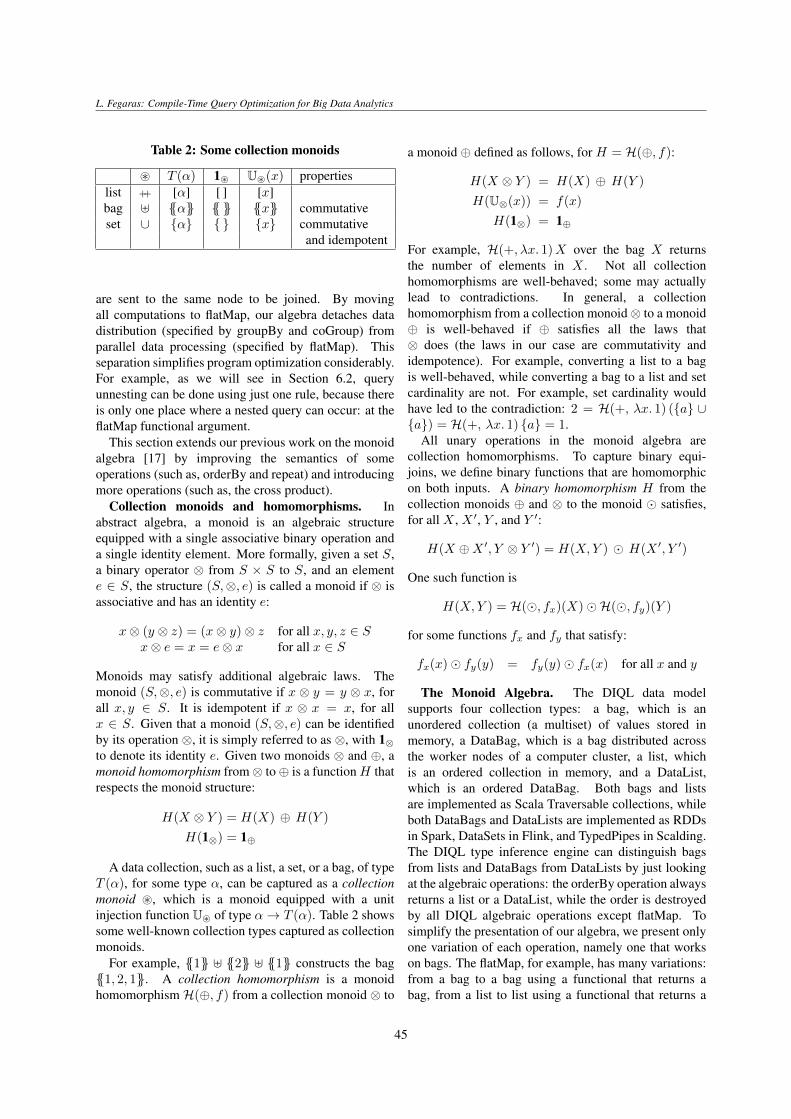
Table 2: Some collection monoids
~ T (α) 1~ U~(x) propertieslist ++ [α] [ ] [x]bag ] {{α}} {{ }} {{x}} commutativeset ∪ {α} { } {x} commutative
and idempotent
are sent to the same node to be joined. By movingall computations to flatMap, our algebra detaches datadistribution (specified by groupBy and coGroup) fromparallel data processing (specified by flatMap). Thisseparation simplifies program optimization considerably.For example, as we will see in Section 6.2, queryunnesting can be done using just one rule, because thereis only one place where a nested query can occur: at theflatMap functional argument.
This section extends our previous work on the monoidalgebra [17] by improving the semantics of someoperations (such as, orderBy and repeat) and introducingmore operations (such as, the cross product).
Collection monoids and homomorphisms. Inabstract algebra, a monoid is an algebraic structureequipped with a single associative binary operation anda single identity element. More formally, given a set S,a binary operator ⊗ from S × S to S, and an elemente ∈ S, the structure (S,⊗, e) is called a monoid if ⊗ isassociative and has an identity e:
x⊗ (y ⊗ z) = (x⊗ y)⊗ z for all x, y, z ∈ Sx⊗ e = x = e⊗ x for all x ∈ S
Monoids may satisfy additional algebraic laws. Themonoid (S,⊗, e) is commutative if x ⊗ y = y ⊗ x, forall x, y ∈ S. It is idempotent if x ⊗ x = x, for allx ∈ S. Given that a monoid (S,⊗, e) can be identifiedby its operation ⊗, it is simply referred to as ⊗, with 1⊗to denote its identity e. Given two monoids ⊗ and ⊕, amonoid homomorphism from⊗ to⊕ is a functionH thatrespects the monoid structure:
H(X ⊗ Y ) = H(X) ⊕ H(Y )
H(1⊗) = 1⊕
A data collection, such as a list, a set, or a bag, of typeT (α), for some type α, can be captured as a collectionmonoid ~, which is a monoid equipped with a unitinjection function U~ of type α→ T (α). Table 2 showssome well-known collection types captured as collectionmonoids.
For example, {{1}} ] {{2}} ] {{1}} constructs the bag{{1, 2, 1}}. A collection homomorphism is a monoidhomomorphism H(⊕, f) from a collection monoid ⊗ to
a monoid ⊕ defined as follows, for H = H(⊕, f):
H(X ⊗ Y ) = H(X) ⊕ H(Y )
H(U⊗(x)) = f(x)
H(1⊗) = 1⊕
For example, H(+, λx. 1)X over the bag X returnsthe number of elements in X . Not all collectionhomomorphisms are well-behaved; some may actuallylead to contradictions. In general, a collectionhomomorphism from a collection monoid⊗ to a monoid⊕ is well-behaved if ⊕ satisfies all the laws that⊗ does (the laws in our case are commutativity andidempotence). For example, converting a list to a bagis well-behaved, while converting a bag to a list and setcardinality are not. For example, set cardinality wouldhave led to the contradiction: 2 = H(+, λx. 1) ({a} ∪{a}) = H(+, λx. 1) {a} = 1.
All unary operations in the monoid algebra arecollection homomorphisms. To capture binary equi-joins, we define binary functions that are homomorphicon both inputs. A binary homomorphism H from thecollection monoids ⊕ and ⊗ to the monoid � satisfies,for all X , X ′, Y , and Y ′:
H(X ⊕X ′, Y ⊗ Y ′) = H(X,Y ) � H(X ′, Y ′)
One such function is
H(X,Y ) = H(�, fx)(X)�H(�, fy)(Y )
for some functions fx and fy that satisfy:
fx(x)� fy(y) = fy(y)� fx(x) for all x and y
The Monoid Algebra. The DIQL data modelsupports four collection types: a bag, which is anunordered collection (a multiset) of values stored inmemory, a DataBag, which is a bag distributed acrossthe worker nodes of a computer cluster, a list, whichis an ordered collection in memory, and a DataList,which is an ordered DataBag. Both bags and listsare implemented as Scala Traversable collections, whileboth DataBags and DataLists are implemented as RDDsin Spark, DataSets in Flink, and TypedPipes in Scalding.The DIQL type inference engine can distinguish bagsfrom lists and DataBags from DataLists by just lookingat the algebraic operations: the orderBy operation alwaysreturns a list or a DataList, while the order is destroyedby all DIQL algebraic operations except flatMap. Tosimplify the presentation of our algebra, we present onlyone variation of each operation, namely one that workson bags. The flatMap, for example, has many variations:from a bag to a bag using a functional that returns abag, from a list to list using a functional that returns a
45

Open Journal of Big Data (OJBD), Volume 5, Issue 1, 2019
list, from a DataBag to a DataBag using a functionalthat returns a bag, etc, but some combinations are notpermitted as they are not well-behaved, such as a flatMapfrom a bag to a list.
The flatMap operation. The first operation, flatMap,generalizes the select, project, join, cross, and unnestoperations of the nested relational algebra. Given twoarbitrary types α and β, the operation flatMap(f,X)over a bag X of type {{α}} applies the function f oftype α → {{β}} to each element of X , yielding one bagfor each element, and then merges these bags to form asingle bag of type {{β}}. It is expressed as follows asa collection homomorphism from the monoid ] to themonoid ]:
flatMap(f,X) , H(], f)X
which is equivalent to the following equations:
flatMap(f,X ] Y ) = flatMap(f,X)]flatMap(f, Y )
flatMap(f, {{a}}) = f(a)flatMap(f, {{ }}) = {{ }}
Many common distributed queries can be written usingflatMaps, including the equi-join X ./p Y :
flatMap(λx. flatMap(λy. if p(x, y) then {{(x, y)}}else {{ }},
Y ),X)
The flatMap operation is the only higher-orderhomomorphic operation in the monoid algebra. Itsfunctional argument can be any Scala function,including a partial function with a refutable pattern. Inthat case, the second flatMap equation becomes a patternmatching that returns an empty bag if the refutablepattern fails to match.
flatMap(λp. e, {{a}})= amatch { case p => e; case => {{ }} }
where λp. e is an anonymous function, expressed as p⇒e in Scala, where p is a Scala pattern and e is a Scalaexpression.
The groupBy operation. Given a type κ thatsupports value equality (=), a type α, and a bag X oftype {{(κ, α)}}, the operation groupBy(X) groups theelements of X by their first component (the group-bykey) and returns a bag of type {{(κ, {{α}})}} (a key-valuemap, also known as an indexed set). It can be expressedas follows as a collection homomorphism:
groupBy(X) , H(m, λ(k, v). {{(k, {{v}})}})X
which is equivalent to the following equations:
groupBy(X ] Y ) = groupBy(X) m groupBy(Y )groupBy({{(k, v)}}) = {{(k, {{v}})}}
groupBy({{ }}) = {{ }}
The monoid m, called indexed set union, is a full outerjoin that merges groups associated with the same keyusing bag union. More specifically, X m Y is a full outerjoin between X and Y that can be defined as followsusing a set-former notation on bags:
X m Y= { (k, a ] b) ||| (k, a) ∈ X, (k′, b) ∈ Y, k = k′ }] { (k, a) ||| (k, a) ∈ X, ∀(k′, b) ∈ Y : k′ 6= k }] { (k, b) ||| (k, b) ∈ Y, ∀(k′, a) ∈ X : k′ 6= k }
The first term joins X and Y on the group-by key and unions together the groups associatedwith the same key, the second term returns theelements of X not joined with Y , and the thirdterm returns the elements of Y not joined with X .For example, groupBy({{(1, “a”), (2, “b”), (1, “c”)}})returns {{(1, {{“a”, “c”}}), (2, {{“b”}})}}.
The orderBy operation. Given a type κ that supportsa total order (≤), a type α, and a bagX of type {{(κ, α)}},the operation orderBy(X) returns a list of type [(κ, α)]sorted by the order-by key κ. It is expressed as followsas a collection homomorphism:
orderBy(X) , H(⇑, λ(k, v). [(k, v)])X
which is equivalent to the following equations:
orderBy(X ] Y ) = orderBy(X) ⇑ orderBy(Y )orderBy({{(k, v)}}) = [(k, v)]
orderBy({{ }}) = [ ]
The monoid ⇑ merges two sorted sequences of type[(κ, α)] to create a new sorted sequence. It can beexpressed as follows using a set-former notation on lists(list comprehensions):
(X1++X2) ⇑ Y = X1 ⇑ (X2 ⇑ Y )
[(k, v)] ⇑ Y = [ (k′, w) ||| (k′, w) ∈ Y, k′ < k ]++ [(k, v)]++ [ (k′, w) ||| (k′, w) ∈ Y, k′ ≥ k ]
[ ] ⇑ Y = Y
The second equation inserts the pair (k, v) into the sortedlist Y , deriving a sorted list.
The reduce operation. Aggregations are capturedby the collection homomorphism reduce(⊕, X), whichaggregates a bagX of type {{α}} using the non-collectionmonoid ⊕ of type α:
reduce(⊕, X) , H(⊕, λx. x)X
46
L. Fegaras: Compile-Time Query Optimization for Big Data Analytics
For example, reduce(+, {{1, 2, 3}}) = 6.The coGroup operation. Although general joins
and cross products can be expressed using nestedflatMaps, we provide a binary homomorphism thatcaptures lossless equi-joins and outer joins. Theoperation coGroup(X,Y ) between a bag X of type{{(κ, α)}} and a bag Y of type {{(κ, β)}} over their firstcomponent of type κ (the join key) returns a bag of type{{(κ, ({{α}}, {{β}}))}}. It is homomorphic on both inputsas it satisfies the law:
coGroup(X1 ]X2, Y1 ] Y2)= coGroup(X1, Y1) l coGroup(X2, Y2)
where the monoid lmerges pairs of bags associated withthe same key.
X l Y = { (k, (a1 ] b1, a2 ] b2))
||| (k, (a1, a2)) ∈ X, (k′, (b1, b2)) ∈ Y, k = k′ }] { (k, p) ||| (k, p) ∈ X, ∀(k′, q) ∈ Y : k′ 6= k }] { (k, q) ||| (k, q) ∈ Y, ∀(k′, p) ∈ X : k′ 6= k }
For example, coGroup( {{(1, 10), (2, 20), (1, 30)}},{{(1, 40), (2, 50), (3, 60)}} ) = {{(1, ({{10, 30}}, {{40}})),(2, ({{20}}, {{50}})), (3, ({{ }}, {{60}}))}}.
The cross product operation, cross(X,Y ) is theCartesian product betweenX of type {{α}} and Y of type{{β}} that returns {{(α, β)}}. Unlike coGroup, it is not amonoid homomorphism:
cross(X1 ]X2, Y1 ] Y2)= cross(X1, Y1) ] cross(X1, Y2)] cross(X2, Y1) ] cross(X2, Y2)
The repeat operation. Given a value X of typeα, a function f of type α→ α, a predicate p oftype α→ boolean, and a counter n, the operationrepeat(f, p, n,X) returns a value of type α. It is definedas follows:
repeat(f, p, n,X) , if n ≤ 0 ∨ ¬p(X)then Xelse repeat(f, p, n− 1, f(X))
The repetition stops when the number of remainingrepetitions is zero or the result value fails to satisfy thecondition p.
5 TRANSLATION OF DIQL TO THE MONOIDALGEBRA
Table 3 presents the rules for translating DIQL queriesto the monoid algebra. The form QJ e K translates theDIQL syntax of e (defined in Table 1) to the monoidalgebra. The notation λp.e, where p is a Scala pattern, isan anonymous function f defined as f(p) = e. Although
the rules in Table 3 translate join queries to nestedflatMaps, in Section 6.2, we present a general methodfor deriving joins from nested flatMaps.
The order that select-queries are translated in Table 3is as follows: the distinct clause is translated first, thenthe order-by clause, then the group-by/having clauses,then the ‘from’ clause (the query qualifiers), then the‘where’ clause, and finally the select header (the queryresult). Rule (1) translates a distinct query to a group-by that removes duplicates by grouping the query resultvalues by the entire value. Rule (2) translates an order-byquery to an orderBy operation.
Rules (3) and (4) translate group-by queries. Recallthat, after group-by, every pattern variable in a queryexcept the group-by pattern variables, are lifted to acollection of values to contain all bindings of thisvariable associated with a group. To specify thesebindings, we use the notation Vp
q to denote the flat tuplethat contains all pattern variables in the sequence ofqualifiers q that do not appear in the group-by patternp. It is defined as Vp
q = (v1, . . . , vn) (the order ofv1, . . . , vn is unimportant), where vi ∈ (VJ q K−PJ p K)and V is defined as follows:
VJ p <− e, q K = PJ p K ∪ VJ q KVJ p <−− e, q K = PJ p K ∪ VJ q KVJ p = e, q K = PJ p K ∪ VJ q K
where PJ p K is the set of pattern variables in the patternp. As a simplification, we lift only the variables that areaccessed by the rest of the query, since all others areignored. The query select (e,Vp
q ) from q in Rules (3)and (4) is the query before the group-by operation thatreturns a collection of pairs that consist of the group-by key and the non-group-by variables Vp
q . Hence,after groupBy, the non-group-by variables are groupedinto a collection to be used by the rest of the query.The operation lift((v1, . . . , vn), s, e), where s is thecollection that contains the values of the non-group-byvariables in the current group, lifts each variable vi to acollection by rebinding it to a collection derived from sas flatMap(λ(v1, . . . , vn). {{vi}}, s).
Rule (5) translates a generator p <− e to a flatMap.Rule (6) is similar, but embeds the annotation ‘small’(which is the identity operation), to be used by theoptimizer as a hint about the collection size. Rule (7)gives the translation of a let-binding for an irrefutablepattern p. For a refutable p, the translation is:
QJ e K match { case p => QJ select e from q Kcase => {{ }} }
Rules (8) and (9) are the last rules to be appliedwhen all qualifiers in the query have been translated,and hence, the ‘from’ clause is empty. Rule (8)
47
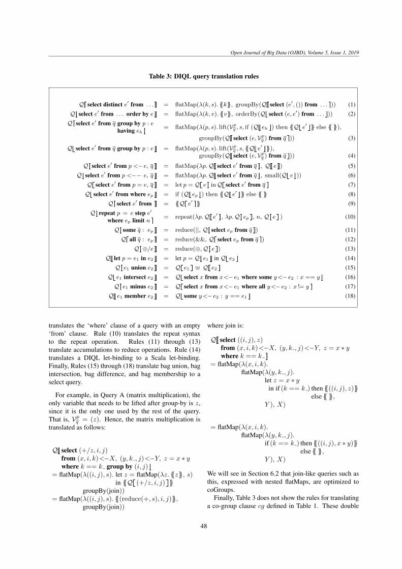
Open Journal of Big Data (OJBD), Volume 5, Issue 1, 2019
Table 3: DIQL query translation rules
QJ select distinct e′ from . . . K = flatMap(λ(k, s). {{k}}, groupBy(QJ select (e′, ()) from . . . K)) (1)
QJ select e′ from . . . order by e K = flatMap(λ(k, v). {{v}}, orderBy(QJ select (e, e′) from . . . K)) (2)
QJ select e′ from q group by p : ehaving eh K
= flatMap(λ(p, s). lift(Vpq , s, if (QJ eh K) then {{QJ e′ K}} else {{ }}),
groupBy(QJ select (e,Vpq ) from q K)) (3)
QJ select e′ from q group by p : e K = flatMap(λ(p, s). lift(Vpq , s, {{QJ e′ K}}),
groupBy(QJ select (e,Vpq ) from q K)) (4)
QJ select e′ from p <− e, q K = flatMap(λp.QJ select e′ from q K, QJ e K) (5)
QJ select e′ from p <−− e, q K = flatMap(λp.QJ select e′ from q K, small(QJ e K)) (6)
QJ select e′ from p = e, q K = let p = QJ e K inQJ select e′ from q K (7)
QJ select e′ from where ep K = if (QJ ep K) then {{QJ e′ K}} else {{ }} (8)
QJ select e′ from K = {{QJ e′ K}} (9)
QJ repeat p = e step e′
where ep limit n K= repeat(λp.QJ e′ K, λp.QJ ep K, n, QJ e K ) (10)
QJ some q : ep K = reduce(||, QJ select ep from q K) (11)
QJ all q : ep K = reduce(&&, QJ select ep from q K) (12)
QJ⊕/e K = reduce(⊕,QJ e K) (13)
QJ let p = e1 in e2 K = let p = QJ e1 K in QJ e2 K (14)
QJ e1 union e2 K = QJ e1 K ] QJ e2 K (15)
QJ e1 intersect e2 K = QJ select x from x<− e1 where some y<− e2 : x == y K (16)
QJ e1 minus e2 K = QJ select x from x<− e1 where all y<− e2 : x != y K (17)
QJ e1 member e2 K = QJ some y<− e2 : y == e1 K (18)
translates the ‘where’ clause of a query with an empty‘from’ clause. Rule (10) translates the repeat syntaxto the repeat operation. Rules (11) through (13)translate accumulations to reduce operations. Rule (14)translates a DIQL let-binding to a Scala let-binding.Finally, Rules (15) through (18) translate bag union, bagintersection, bag difference, and bag membership to aselect query.
For example, in Query A (matrix multiplication), theonly variable that needs to be lifted after group-by is z,since it is the only one used by the rest of the query.That is, Vp
q = (z). Hence, the matrix multiplication istranslated as follows:
QJ select (+/z, i, j)from (x, i, k)<−X, (y, k , j)<−Y, z = x ∗ ywhere k == k group by (i, j) K
= flatMap(λ((i, j), s). let z = flatMap(λz. {{z}}, s)in {{QJ (+/z, i, j) K}}
groupBy(join))= flatMap(λ((i, j), s). {{(reduce(+, s), i, j)}},
groupBy(join))
where join is:
QJ select ((i, j), z)from (x, i, k)<−X, (y, k , j)<−Y, z = x ∗ ywhere k == k K
= flatMap(λ(x, i, k).flatMap(λ(y, k , j).
let z = x ∗ yin if (k == k ) then {{((i, j), z)}}
else {{ }},Y ), X)
= flatMap(λ(x, i, k).flatMap(λ(y, k , j).
if (k == k ) then {{((i, j), x ∗ y)}}else {{ }},
Y ), X)
We will see in Section 6.2 that join-like queries such asthis, expressed with nested flatMaps, are optimized tocoGroups.
Finally, Table 3 does not show the rules for translatinga co-group clause cg defined in Table 1. These double
48
L. Fegaras: Compile-Time Query Optimization for Big Data Analytics
group-by clauses are translating to coGroups using thefollowing rule:
QJ select e′ from q1 group by p1 : e1from q2 group by p2 : e2 K
= flatMap(λ((p1, p2), (s1, s2)).lift(Vp1
q1, s1, lift(Vp2
q2, s2, {{QJ e′ K}})),
coGroup(QJ select (e1,Vp1
q1) from q1 K,
QJ select (e2,Vp2
q2) from q2 K))
For example, for Query B (matrix addition), we haveVp1
q1= (x) and Vp2
q2= (y). Consequently, Query B is
translated as follows:
flatMap(λ(((x, i, j), (y, i , j )), (s1, s2)).let x = flatMap(λ(x, i, j). {{x}}, s1),y = flatMap(λ(y, i , j ). {{y}}, s2)
in {{(+/(x++y), i, j)}},coGroup(A,B))
where A = QJ select ((i, j), x) from (x, i, j) <− X K= flatMap(λ(x, i, j). {{((i, j), x)}}, X) and, similarly,B = QJ select ((i , j ), y) from (y, i , j ) <− Y K= flatMap(λ(y, i , j ). {{((i , j ), y)}}, Y ).
6 QUERY OPTIMIZATION
Given a DIQL query, our goal is to translate it intoan algebraic form that can be evaluated efficiently in aDISC platform. Current database technology has alreadyaddressed this problem in the context of relationaldatabases. The DIQL data model and algebra thoughare richer than those of a relational system, requiringmore general optimization techniques. The relationalalgebra, for instance, as well as the algebraic operatorsused by current relational engines, such as Calcite [9],cannot express nested queries, such as a query inside aselection predicate, thus requiring the query translatorto unnest queries using source-to-source transformationsbefore the queries are translated to algebraic terms. Thislimitation may discourage language designers to supportnested queries, although they are very common in DISCdata analysis (for example, the k-means clustering query(Query E)).
Currently, our optimizations are not based on anycost model; instead, they are heuristics that take intoaccount the hints provided by the user, such as usinga <-- qualifier to traverse a small dataset. That is,our framework tries to identify all possible joins andconvert them to broadcast joins if they are over a smalldataset, but currently, it does not optimize the joinorder. In this section, we present the normalization rulesthat put DIQL terms to a canonical form (Section 6.1),a general method for query unnesting (Section 6.2),pushing down predicates (Section 6.3), and columnpruning (Section 6.4).
6.1 Query Simplification
Cascaded flatMaps can be fused into a single nestedflatMap using the following law that is well-known infunctional PLs:
flatMap(f, flatMap(g, S))
→ flatMap(λx. flatMap(f, g(x)), S) (19)
If S is a distributed dataset, this normalization rulereduces the number of required distributed operationsfrom two to one and eliminates redundant operationsif we apply further optimizations to the inner flatMap.It generalizes well-known algebraic laws in relationalalgebra, such as fusing two cascaded selections intoone. If we apply this transformation repeatedly, anyalgebraic term can be normalized into a tree of groupBy,coGroup, and cross operations with a single flatMapbetween each pair of these operations. There are manyother standard normalization rules, such as projectingover a tuple, (e1, . . . , en). i = ei, and rules that arederived directly from the operator’s definition, such asflatMap(f, {{a}}) = f(a).
6.2 Deriving Joins and Unnesting Queries
The translation rules from the DIQL syntax to themonoid algebra, presented in Section 5, translate join-like queries to nested flatMaps, instead of coGroups. Inthis section, we present a general method for identifyingany possible equi-join from nested flatMaps, includingjoins across deeply nested queries. (An equi-join isa join between two datasets X and Y whose joinpredicate takes the form k1(x) = k2(y), for x ∈ Xand y ∈ Y , for some key functions k1 and k2.) Itis exactly because of these deeply nested queries thatwe have introduced the coGroup operation, because, aswe will see, nested queries over bags are equivalent toouter joins. Translating nested flatMaps to coGroups iscrucial for good performance in distributed processing.Without joins, the only way to evaluate a nested flatMap,such as flatMap(λx. flatMap(λy. h(x, y), Y ), X), ina distributed environment, where both collections Xand Y are distributed, would be to broadcast the entirecollection Y across the processing nodes so that eachprocessing node would join its own partition of X withthe entire dataset Y . This is a good evaluation plan ifY is small. By mapping a nested flatMap to a coGroup,we create opportunities for more evaluation strategies,which may include the broadcast solution. For example,one good evaluation strategy for large X and Y that arejoined via the key functions k1 and k2, is to partitionX by k1, partition Y by k2, and shuffle these partitionsto the processing nodes so that data with matching keyswill go to the same processing node. This is called a
49
Open Journal of Big Data (OJBD), Volume 5, Issue 1, 2019
distributed partitioned join. While related approachesfor query unnesting [19, 23] require many rewrite rulesto handle various cases of query nesting, our methodrequires only one rule and is more general as it handlesnested queries of any form and any number of nestinglevels.
Consider the following DIQL query over X and Y :
Query F:select bfrom (a,b) <− Xwhere b > +/(select d from (c,d) <− Y
where a==c)
One efficient method for evaluating this nested query isto first group Y by its first component and aggregate:
Z = select (c,+/d) from (c,d) <− Y group by c
and then to join X with Z:
Query G:select bfrom (a,b) <− X, (c,sum) <− Zwhere a==c && b>sum
This query though is not equivalent to the originalQuery F; if an element of X has no matches in Y, thenthis element will appear in the result of Query F (sincethe sum over an empty bag is 0), but it will not appear inthe result of Query G (since it does not satisfy the joincondition). To correct this error, Query G should use aleft-outer join between X and Z. In other words, using themonoid algebra, we want to translate query Query F to:
flatMap(λ(k, (xs, ys)).flatMap(λb.
if (b > reduce(+, ys))
then {{b}} else {{ }}, xs)coGroup(flatMap(λ(a, b). {{(a, b)}}, X),
flatMap(λ(c, d). {{(c, d)}}, Y )))
That is, the query unnesting is done with a left-outer join,which is captured concisely by the coGroup operationwithout the need for using an additional group-byoperation or handling null values.
We now generalize the previous example to convertnested flatMaps to joins. We consider patterns ofalgebraic terms of the form:
flatMap(λp1. g(flatMap(λp2. e, e2)), e1) (20)
for some patterns p1 and p2, some terms e1, e2, ande, and some term function g. (A term function is analgebraic term that contains its arguments as subterms.)For the cases we consider, the term e2 should not dependon the pattern variables in p1, otherwise it would notbe a join. This algebraic term matches most pairs ofnested flatMaps on bags that are equivalent to joins,
including those derived from nested queries, such as theprevious DIQL query, and those derived from flat join-like queries. Thus, the method presented here detectsand converts any possible join to a coGroup.
We consider the following term function (derived fromthe term (20)) as a candidate for a join:
F (X,Y ) =
flatMap(λp1. g(flatMap(λp2. e, Y )), X) (21)
We require that g({{ }}) = {{ }}, so that F (X,Y ) = {{ }} ifeither X or Y is empty. To transform F (X,Y ) to a joinbetween X and Y , we need to derive two terms k1 andk2 from e (these are the join keys), such that k1 6= k2implies e = {{ }}, and k1 depends on the p1 variableswhile k2 depends on the p2 variables, exclusively. Then,if there are such terms k1 and k2, we transform F (X,Y )to the following join:
F ′(X,Y ) =
flatMap(λ(k, (xs, ys)). F (xs, ys), (22)coGroup(flatMap(λx@p1. {{(k1, x)}}, X),
flatMap(λy@p2. {{(k2, y)}}, Y )))
(Recall that the Scala pattern binder x@pmatches a valuewith the pattern p and binds x to that value.) The proofthat F ′(X,Y ) = F (X,Y ) is given in Theorem A.1in the Appendix. This is the only transformation ruleneeded to derive any possible join from a query andunnest nested queries because there is only one higher-order operator in the monoid algebra (flatMap) that cancontain a nested query.
For example, consider Query F again:
select bfrom (a, b)<−Xwhere b > +/(select d from (c, d)<−Y
where a == c)
It is translated to the following algebraic term Q(X,Y ):
flatMap(λ(a, b). if (b > reduce(+,flatMap(N, Y ))then {{b}} else {{ }}, X)
where N = λ(c, d). if (a == c) then {{d}} else {{ }}.This term matches the term function F (X,Y )in Equation (21) using g(z) = if (b >reduce(+, z)) then {{b}} else {{ }} and e = if (a ==c) then {{d}} else {{ }}. We can see that k1 = a andk2 = c because a 6= c implies e = {{ }}. Thus, fromEquation (22), Q(X,Y ) is transformed to:
flatMap(λ(k, (xs, ys)). Q(xs, ys),coGroup(flatMap(λx@(a, b). {{(a, x)}}, X),
flatMap(λy@(c, d). {{(c, y)}}, Y )))
50
L. Fegaras: Compile-Time Query Optimization for Big Data Analytics
The biggest challenge in applying the transformationin Equation (22) is to derive the join keys, k1 and k2,from the term e. If flatMaps are normalized first usingEquation (19), then the only place these key functionscan appear is in a flatMap functional argument. Then, thebody of the flatMap functional argument can be anotherflatMap, in which case we consider the latter flatMap, ora term if p then e′ else {{ }}, in which case we derive thekeys from p, such that k1 6= k2 ⇒ ¬p. If p is alreadyin the form k1 == k2, then, in addition to deriving thekeys k1 and k2, we can simplify the term F (xs, ys) inEquation (22) by replacing the term if p then e′ else {{ }}with e′.
Finally, the term F ′(X,Y ) in Equation (22) assumesthat we can derive a pair of keys, k1 and k2, such thatk1 depends only on p1, and k2 depends only on p2.But, often, such keys do not exists because they dependon variable bindings introduced inside the term functiong and the term e. In such cases, calculating the keysbefore coGroup using flatMap(λx@p1. {{(k1, x)}}, X)and flatMap(λy@p2. {{(k2, y)}}, Y ), would be incorrectbecause the terms k1 and k2 would depend on additionalvariables. To compensate, we collect all operations in gand e that introduce new bindings, namely flatMaps, intotwo corrective term functions, mx and my , to bind thevariables used by the keys k1 and k2, respectively. Morespecifically, the coGroup in Equation (22) will become:
coGroup(flatMap(λ[email protected]({{(k1, x)}}), X),flatMap(λ[email protected]({{(k2, y)}}), Y ))
Starting with an initial set of variables Vx = PJ p1 K andmx = λx. x for X , and Vy = PJ p2 K and my = λy. yfor Y , we consider every flatMap(λp. b, e) in the termsg and e that leads to the keys k1 and k2. If the term edepends on the variables in Vx only, then Vx ← Vx ∪PJ p K and mx ← λx. flatMap(λp.mx(x), e). If theterm e depends on the variables in Vy only, then Vy ←Vy ∪ PJ p K and my ← λy.flatMap(λp.my(y), e).Otherwise, if the term e depends on the variables inboth Vx and Vy , then it is impossible to derive acoGroup because we cannot calculate each one of thekeys separately.
6.3 Pushing Down Predicates
One important optimization technique used in relationaldatabases is pushing selections before joins. We havegeneralized this technique to apply to nested datacollections and complex queries. This technique uses thefunction split that splits a predicate into two predicates:given a predicate c and a set of variables V , splitJ c KVreturns a pair (c1, c2) such that c1 ∧ c2 ⇒ c and c1 maydepend on the variables in V while c2 must not.
The first optimization is pushing filters before agroupBy:
flatMap(λ(k, s). g(flatMap(λp. h(if c then e′
else {{ }}, s))),groupBy(e))
= flatMap(λ(k, s). g(flatMap(λp. h(if c2 then e′
else {{ }}, s))),groupBy(flatMap(λ(k, x@p). if c1 then {{x}}
else {{ }},e)))
where g and h are term functions with g({{ }}) =h({{ }}) = {{ }}. That is, part of the filter’s condition c1after the groupBy was applied before the groupBy. Here,(c1, c2) = splitJ c KV where V = PJ p K∪{k}, that is, c1may depend on k or the variables in p only. As in the joinderivation algorithm, if g and h introduce new bindingsthrough flatMaps, the flatMap before groupBy shouldbe wrapped with a corrective term function to bind thevariables used by these flatMaps.
Pushing a filter into the left input of a coGroupis done using the following transformation (a similartransformation exists for the right input):
flatMap(λ(k, (xs, ys)).g(flatMap(λp. h(if c then e′
else {{ }}, xs)),coGroup(e1, e2))
= flatMap(λ(k, (xs, ys)).g(flatMap(λp. h(if c2 then e′
else {{ }}, xs)),coGroup(flatMap(λ(k, x@p). if c1 then {{x}}
else {{ }},e1),
e2))
where, here, c1 may depend on k or the variables in ponly.
For example, consider the following query:
Query H:select (b,d)from (a,b) <− X, (c,d) <− Ywhere a==c && b>3
which is translated and optimized to a coGroup based onthe transformations in Section 6.2:
flatMap(λ(k, (xs, ys)).flatMap(λx@(a, b).flatMap(λy@(c, d).
if (b > 3) then {{(b, d)}} else {{ }},ys), xs),
coGroup(flatMap(λx@(a, b). {{(a, x)}}, X)flatMap(λy@(c, d). {{(c, y)}}, Y ))
51
Open Journal of Big Data (OJBD), Volume 5, Issue 1, 2019
Then, using the previous transformation, the (b > 3)condition is pushed into the left input of the coGroup:
flatMap(λ(k, (xs, ys)).flatMap(λx@(a, b).flatMap(λy@(c, d).{{(b, d)}}, ys), xs),
coGroup(flatMap(λx@(a, b). if (b > 3)then {{(a, x)}}else {{ }}, X)
flatMap(λy@(c, d). {{(c, y)}}, Y ))
6.4 Column Pruning
Column pruning is an important optimization forrelational database queries because it reduces the sizeof intermediate results between operations. It is evenmore important for DISC frameworks since it reducesthe amount of shuffled data, which is the prominent costfactor for distributed processing. We have developed ageneral data pruning method that removes unneeded datafrom complex data, which may be nested in arbitraryways. Earlier work on complex data pruning [1] has useda holistic approach to analyze Spark programs writtenin Scala to identify unneeded data components and totransform these programs in such a way that they prunethese data early. Unlike this earlier work, our workuses compositional rules to introduce a flatMap beforeeach groupBy and coGroup that prunes only the parts ofthe data that are not used by the next operation. Thisnewly introduced flatMap is then fused with the existingflatMap in the groupBy or coGroup input. By applyingthis transformation top-down, starting from the queryresult, we minimize the amount of shuffled data, oneoperation at a time.
We consider terms of the form:
flatMap(f, groupBy(e))
Terms with a coGroup can be handled in a similar way.We want to embed a flatMap before the groupBy thatprunes all the data not used by the function f . Let{{(k, tp)}} be the type of e. We want to find all thecomponents of the type tp that are not accessed bythe function f (the group-by key of type k cannot bepruned). We are using a heuristic method that workswell for most cases. We construct a simple instance ofthe type tp, using IJ tp K, defined as follows:
IJ {{t}} K = {{IJ t K}}IJ (t1, . . . , tn) K = (IJ t1 K, . . . , IJ tn K)
IJ t K = vt a basic type
where vt is a new variable of type t. There are morecases that are not included here. If we optimize theterm f((k, IJ {{tp}} K)) using the normalization rules
presented in Section 6.1, then, if the variable vtassociated with a type t does not occur in the resultingnormalized term, then it is not accessed by f . In thatcase, we call this type t an unused type. For example, let
f = λ(k, s). reduce(+,flatMap(λ(x, y).{{y}}, s))
and let the type tp be (int, int). Then, IJ {{tp}} K ={{(v1, v2)}}, where v1 corresponds to the first int and v2to the second. The normalized term f((k, {{(v1, v2)}}))is reduce(+, {{v2}}), which means that only the secondint from the type (int, int) is used.
Based on the type annotations on the terms thatrepresent basic types in tp (used or unused), we annotateall the subterms of the term tp: a type List[t] is unusedif t is unused, and a type (t1, . . . , tn) is unused if allt1, . . . , tn are unused. Given that every subterm in tp ismarked as used or unused, we generate code (a function)that prunes all unused data from the input:
C1J t K = λx. () if t is unusedC1J {{t}} K = λx. flatMap(λz. {{C1J t K(z)}}, x)C1J (t1, . . . , tn) K
= λ(v1, . . . , vn). (C1J ti1 K(vi1), . . . , C1J tim K(vim))for the used types ti1 , . . . , tim
C1J t K = λx. x otherwise
and a similar function C2J t K (not shown) that convertsthe pruned data to a t value by embedding the value() in the place of the unused components, so thatC1J t K(C2J t Kx) = x, for every x of type t. Then, C1is used to deeply prune data before the groupBy, whileC2 is used to insert () values after groupBy:
flatMap(f, groupBy(e))= flatMap(f, flatMap(λ(k, s). {{(k, C2J {{tp}} K s)}},
groupBy(flatMap(λ(k, x). {{(k, C1J tp Kx)}},e))))
After the top two flatMap operations are fused usingEquation (19), these () values are eliminated since theyare not used by f . Based on the previous example,C1J (int, int) K = λ(v1, v2). v2 and C2J {{(int, int)}} K =λx. flatMap(λv2. {{((), v2)}}, x). Thus, the datapruning is flatMap(λ(k, x). {{(k, C1J tp Kx)}}, e) beforegroupBy, which is equal to flatMap(λ(k, (v1, v2)).{{(k, v2}}, e), for x = (v1, v2). That is, it prunes thefirst column before groupBy.
7 IMPLEMENTATION
DIQL generates Scala code, which is translated to JVMbyte code at compile-time using Scala’s compile-timereflection facilities. This code generation is vastlysimplified with the use of quasiquotes, which allow one
52
L. Fegaras: Compile-Time Query Optimization for Big Data Analytics
to construct internal Scala abstract syntax trees (ASTs)by just embedding Scala syntax in quotes. After a DIQLquery is parsed, it is translated to an AST. DIQL ASTsare a subset of Scala’s ASTs for expressions and patterns,since they need to capture Scala’s purely functionalsyntax only, but are extended with special nodes tocapture our algebraic operators. Figure 1 shows thequery translation process at compile time.
The DIQL data model extends Scala’s types with fourcollection types: bag, list, DataBag, and DataList. TheDIQL code generator needs to know which collectiontypes are used by the algebraic operations to decidewhich API to use for each operation. In addition,many optimizations apply only when the operationsinvolved are over distributed datasets, which requiresknowledge about the types. To determine the kindof collections used by the algebraic operations, theDIQL type inference system uses the Scala type checker.All Scala Traversable objects (that is, instances ofclasses that conform to the type Traversable, suchas a List) are in-memory collections (bags or lists).Instances of distributed collection classes supported bythe underlying distributed framework are distributedcollections (DataBags or DataLists). For Spark, forexample, instances of classes that conform to the classRDD (such as, an RDD or any subclass of RDD) aretaken to be distributed collections. Furthermore, theDIQL type inference engine distinguishes bags fromlists and DataBags from DataLists by just looking atthe algebraic operations: the orderBy operation alwaysreturns a list or a DataList, while the order is destroyedby all monoid algebraic operations except flatMap. Abag (resp. a DataBag) is more restricted than a list(resp. a DataList) as it does not permit certain operationsthat depend on order, such as indexing.
In Section 4, to simplify the presentation, wepresented only one variation of each algebraic operation,namely one that works on bags. But there are multiplevariations of some operations. The flatMap, for example,has many variations: from a bag to a bag using afunctional that returns a bag, from a list to list usinga functional that returns a list, from a DataBag to aDataBag using a functional that returns a bag, etc, butsome combinations are not permitted as they are notwell-behaved, such as a flatMap from a bag to a list.
The DIQL type inference system extends the Scalatype inference system using a very simple trick: DIQLgenerates Scala code and the code is type-checkedusing Scala’s compile-time reflection facilities. Morespecifically, the DIQL type-checker uses a typingenvironment that binds Scala patterns to Scala types.When type-checking a DIQL algebraic term e under atyping environment that consists of the bindings p1 :t1, . . . , pn : tn, which bind the patterns pi to their types
ti, it calls the DIQL code generator to generate a ScalaAST c from the term e and then it calls the Scala type-checker to get the type of the Scala code
(p1 : t1) => · · · (pn : tn) => c
which will derive a functional type t1 → · · · tn → t,for some type t, provided that the code c is type-correct.This type t is then the type of e. The typing environmentis extended during the type-checking of a DIQL queryand of the algebraic operators derived from the query.In Spark, for instance, the type t of the term e2 inflatMap(λp. e1, e2) must conform to the class RDD[t′]or to the class Traversable[t′], for some type t′. Thenthe functional body e1 is type-checked using the currenttyping environment extended with the binding p : t′.
The DIQL optimizer finds all possible joins and crossproducts, optimizes the algebraic terms, then factors outall common terms (so that their value is cached at run-time), and finally generates broadcast operations for thein-memory operations that are accessed in the functionalparameter of a flatMap over a DataBag. CoGroupsand cross products between a distributed DataBag anda ‘small’ DataBag (as defined by the<−− qualifier) oran in-memory bag, are translated to broadcast joins andcross products, which broadcast the small dataset to allworkers.
Not all nested flatMaps on DataBags can be translatedto coGroups and cross products. For example, DIQLevaluates the following query on the DataBags S and R:
select ( x, +/(select w from (z,w) <− R where z<y) )from (x,y) <− S
by broadcasting R to all worker nodes.DIQL abstracts a DISC platform using an abstract
class that is parameterized by a type constructor DataBag(these are called higher kinded types in Scala, and aretype constructors that take type constructors as typeparameters):
abstract class DistrCodeGen[DataBag[ ]]
which defines an abstract method for each DIQLoperator:
def flatMap[A,B]( f : (A) => Traversable[B], S: DataBag[A] )( implicit tag: ClassTag[B]): DataBag[B]
where the implicit tag is required by all DISC Scala APIsto allow run-time reflection. For example, the Spark codegenerator binds DataBag to RDD:
class SparkCodeGenerator extends DistrCodeGen[RDD]
and implements the abstract methods based on RDDs.That way, the DIQL code generator is modularized andis very easy to extend to multiple DISC platforms. Outof the 4560 lines of the DIQL implementation, the codegenerator for Spark is 468 lines, for Flink is 570 lines,and for Scalding is 386 lines.
53
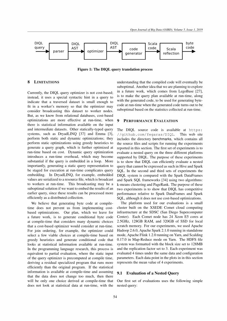
Open Journal of Big Data (OJBD), Volume 5, Issue 1, 2019
Figure 1: The DIQL query translation process
8 LIMITATIONS
Currently, the DIQL query optimizer is not cost-based;instead, it uses a special syntactic hint in a query toindicate that a traversed dataset is small enough tofit in a worker’s memory so that the optimizer mayconsider broadcasting this dataset to worker nodes.But, as we know from relational databases, cost-basedoptimizations are more effective at run-time, whenthere is statistical information available on the inputand intermediate datasets. Other statically-typed querysystems, such as DryadLINQ [37] and Emma [3],perform both static and dynamic optimizations; theyperform static optimizations using greedy heuristics togenerate a query graph, which is further optimized atrun-time based on cost. Dynamic query optimizationintroduces a run-time overhead, which may becomesubstantial if the query is embedded in a loop. Moreimportantly, generating a static query representation tobe staged for execution at run-time complicates queryembedding. In DryadLINQ, for example, embeddedvalues are serialized to a resource file, which is broadcastto workers at run-time. This broadcasting may be asuboptimal solution if we want to embed the results of anearlier query, since these results can be processed moreefficiently as a distributed collection.
We believe that generating byte code at compile-time does not prevent us from implementing cost-based optimizations. Our plan, which we leave fora future work, is to generate conditional byte codeat compile-time that considers many dynamic choicesthat a cost-based optimizer would consider at run-time.For join ordering, for example, the optimizer couldselect a few viable choices at compile-time based ongreedy heuristics and generate conditional code thatlooks at statistical information available at run-time.In the programming language research, this process isequivalent to partial evaluation, where the static inputof the query optimizer is precomputed at compile time,deriving a residual specialized program that runs moreefficiently than the original program. If the statisticalinformation is available at compile-time and assumingthat the data does not change too much, then therewill be only one choice derived at compile-time thatdoes not look at statistical data at run-time, with the
understanding that the compiled code will eventually besuboptimal. Another idea that we are planning to explorein a future work, which comes from LegoBase [27],is to make the query plan available at run-time, alongwith the generated code, to be used for generating byte-code at run-time when the generated code turns out to besuboptimal based on the statistics collected at run-time.
9 PERFORMANCE EVALUATION
The DIQL source code is available at https://github.com/fegaras/DIQL. This web siteincludes the directory benchmarks, which contains allthe source files and scripts for running the experimentsreported in this section. The first set of experiments is toevaluate a nested query on the three different platformssupported by DIQL. The purpose of these experimentsis to show that DIQL can efficiently evaluate a nestedquery that cannot be expressed as such in Hive and SparkSQL. In the second and third sets of experiments theDIQL system is compared with the Spark DataFramesand Spark SQL frameworks [34] using two algorithms:k-means clustering and PageRank. The purpose of thesetwo experiments is to show that DIQL has competitiveperformance relative to Spark DataFrames and SparkSQL, although it does not use cost-based optimizations.
The platform used for our evaluations is a smallcluster built on the XSEDE Comet cloud computinginfrastructure at the SDSC (San Diego SupercomputerCenter). Each Comet node has 24 Xeon E5 cores at2.5GHz, 128GB RAM, and 320GB of SSD for localscratch memory. For our experiments, we used ApacheHadoop 2.6.0, Apache Spark 2.1.0 running in standalonemode, Apache Flink 1.2.0 running on Yarn, and Scalding0.17.0 in Map-Reduce mode on Yarn. The HDFS filesystem was formatted with the block size set to 128MBand the replication factor set to 3. Each experiment wasevaluated 4 times under the same data and configurationparameters. Each data point in the plots in in this sectionrepresents the mean value of 4 experiments.
9.1 Evaluation of a Nested Query
Our first set of evaluations uses the following simplenested query:
54
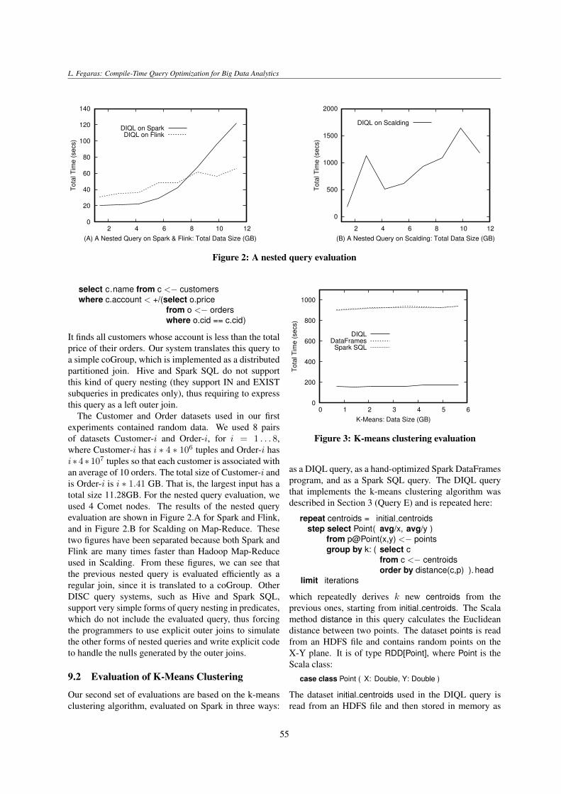
L. Fegaras: Compile-Time Query Optimization for Big Data Analytics
0
20
40
60
80
100
120
140
2 4 6 8 10 12
Tota
l T
ime (
se
cs)
(A) A Nested Query on Spark & Flink: Total Data Size (GB)
DIQL on SparkDIQL on Flink
0
500
1000
1500
2000
2 4 6 8 10 12
Tota
l T
ime (
se
cs)
(B) A Nested Query on Scalding: Total Data Size (GB)
DIQL on Scalding
Figure 2: A nested query evaluation
select c.name from c <− customerswhere c.account < +/(select o.price
from o <− orderswhere o.cid == c.cid)
It finds all customers whose account is less than the totalprice of their orders. Our system translates this query toa simple coGroup, which is implemented as a distributedpartitioned join. Hive and Spark SQL do not supportthis kind of query nesting (they support IN and EXISTsubqueries in predicates only), thus requiring to expressthis query as a left outer join.
The Customer and Order datasets used in our firstexperiments contained random data. We used 8 pairsof datasets Customer-i and Order-i, for i = 1 . . . 8,where Customer-i has i ∗ 4 ∗ 106 tuples and Order-i hasi∗4∗107 tuples so that each customer is associated withan average of 10 orders. The total size of Customer-i andis Order-i is i ∗ 1.41 GB. That is, the largest input has atotal size 11.28GB. For the nested query evaluation, weused 4 Comet nodes. The results of the nested queryevaluation are shown in Figure 2.A for Spark and Flink,and in Figure 2.B for Scalding on Map-Reduce. Thesetwo figures have been separated because both Spark andFlink are many times faster than Hadoop Map-Reduceused in Scalding. From these figures, we can see thatthe previous nested query is evaluated efficiently as aregular join, since it is translated to a coGroup. OtherDISC query systems, such as Hive and Spark SQL,support very simple forms of query nesting in predicates,which do not include the evaluated query, thus forcingthe programmers to use explicit outer joins to simulatethe other forms of nested queries and write explicit codeto handle the nulls generated by the outer joins.
9.2 Evaluation of K-Means Clustering
Our second set of evaluations are based on the k-meansclustering algorithm, evaluated on Spark in three ways:
0
200
400
600
800
1000
0 1 2 3 4 5 6
Tota
l T
ime (
secs)
K-Means: Data Size (GB)
DIQLDataFrames
Spark SQL
Figure 3: K-means clustering evaluation
as a DIQL query, as a hand-optimized Spark DataFramesprogram, and as a Spark SQL query. The DIQL querythat implements the k-means clustering algorithm wasdescribed in Section 3 (Query E) and is repeated here:
repeat centroids = initial centroidsstep select Point( avg/x, avg/y )
from p@Point(x,y) <− pointsgroup by k: ( select c
from c <− centroidsorder by distance(c,p) ). head
limit iterations
which repeatedly derives k new centroids from theprevious ones, starting from initial centroids. The Scalamethod distance in this query calculates the Euclideandistance between two points. The dataset points is readfrom an HDFS file and contains random points on theX-Y plane. It is of type RDD[Point], where Point is theScala class:
case class Point ( X: Double, Y: Double )
The dataset initial centroids used in the DIQL query isread from an HDFS file and then stored in memory as
55
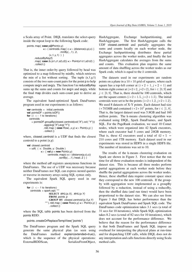
Open Journal of Big Data (OJBD), Volume 5, Issue 1, 2019
a Scala array of Point. DIQL translates the select-queryinside the repeat loop to the following Spark code:
points.map{ case p@Point(x,y)=> ( centroids.map{ c => (distance(c,p),c) }
.minBy( . 1). 2,(x,1,y,1) ) }
.reduceByKey(f)
.map{ case (k,(s1,c1,s2,c2)) => Point(s1/c1,s2/c2) }
. collect ()
That is, the inner order-by query followed by head wasoptimized to a map followed by minBy, which retrievesthe min of a list without sorting. The tuple (x,1,y,1)consists of the two sum-count pairs for the point p to helpcompute avg/x and avg/y. The function f in reduceByKeysums up the sums and counts for avg/x and avg/y, whilethe final map divides each sum-count pair to derive anaverage.
The equivalent hand-optimized Spark DataFramesprogram used in our experiments is as follows:
var centroids = initial centroidsval pointsDF = points.toDF()for ( i <− 1 to iterations )
centroids= pointsDF.groupBy(closest centroid(col(”X”),col( ”Y” )))
.agg(avg(”X”),avg(”Y”))
.rdd.map { case Row( ,x,y) => Point(x,y) }
. collect ()
where, closest centroid is a UDF that finds the closestcentroid to a point (x,y):
val closest centroid= udf( ( x: Double, y: Double )
=> { val p = new Point(x,y)centroids.map(c => (distance(p,c),c))
.sortBy( . 1 ). head. 2 } )
where the method udf registers anonymous functions inDataFrames. The use of a UDF was necessary becauseneither DataFrames nor SQL can express nested queriesor traverse in-memory arrays using SQL syntax only.
The equivalent Spark SQL query used in ourexperiments is:
for ( i <− 1 to iterations )centroids = spark.sql( ”””
SELECT AVG(p.X), AVG(p.Y)FROM points pGROUP BY closest centroid (p.X,p.Y)
””” ). rdd.map { case Row(x,y) => Point(x,y) }. collect ()
where the SQL table points has been derived from thepoints RDD:
points.createOrReplaceTempView(”points”)
The DataFrames program and the Spark SQL querygenerate the same physical plan (as seen usingthe DataFrames method explain(extended=true)),which is the sequence of the physical operations:ExternalRDDScan, SerializeFromObject,
HashAggregate, Exchange hashpartitioning, andHashAggregate. The first HashAggregate calls theUDF closest centroid and partially aggregates thesums and counts locally on each worker node, theExchange hashpartitioning distributes these partialaggregates across the worker nodes, and finally the lastHashAggregate calculates the averages from the sumsand counts. This evaluation plan requires the sameamount of data shuffling across the worker nodes as ourSpark code, which is equal to the k centroids.
The datasets used in our experiments are randompoints on a plane in a 10×10 grid of squares, where eachsquare has a top-left corner at (i ∗ 2 + 1, j ∗ 2 + 1) andbottom-right corner at (i∗2+2, j∗2+2), for i ∈ [0, 9] andj ∈ [0, 9]. That is, there should be 100 centroids, whichare the square centers (i∗2+1.5, j ∗2+1.5). The initialcentroids were set to be the points (i∗2+1.2, j∗2+1.2).We used 8 datasets of X-Y points. Each dataset had sizei ∗ 705MB and contained i ∗ 2 ∗ 107 points, for i ∈ [1, 8].That is, the largest dataset used was 5.8GB and had 160million points. The k-means clustering algorithm wasevaluated using DIQL, Spark DataFrames, and SparkSQL. For the PageRank evaluation, we used 10 Cometnodes, which were organized into 42 Spark executors,where each executor had 5 cores and 24GB memory.That is, these 42 executors used a total of 42 ∗ 5 =210 cores and 1TB memory. Each dataset used in ourexperiments was stored in HDFS in a single HDFS file.The number of iterations was set to 10.
The results of the k-means clustering evaluation onSpark are shown in Figure 3. First notice that the runtime for all three evaluation modes is independent of thedataset size. This is because all three modes performpartial aggregations at each worker node before theyshuffle the partial aggregations across the worker nodes.Hence, these shuffled data require constant space sincethey correspond to the new 100 centroids. If the group-by with aggregation were implemented as a groupByfollowed by a reduction, instead of using a reduceBy,then the shuffled data (and run time) would have beenproportional to the dataset size. We can also see fromFigure 3 that DIQL has better performance than theequivalent Spark DataFrames and Spark SQL code. TheDataFrames code optimization takes 3.1 secs (a total of31 secs for 10 iterations), while Spark SQL optimizationtakes 8.2 secs (a total of 82 secs for 10 iterations), whichdoes not account for the performance difference. Webelieve that the reason for the performance differenceis that both DataFrames and Spark SQL impose anoverhead for interpreting the physical plans at run-timeand for dispatching UDF calls, while DIQL does not doany interpretation and calls functions directly using Scalamethod calls.
56
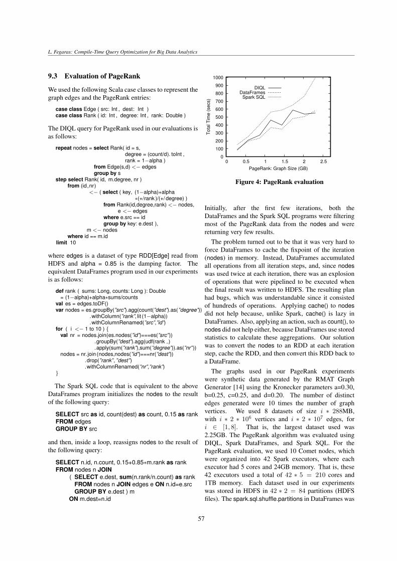
L. Fegaras: Compile-Time Query Optimization for Big Data Analytics
9.3 Evaluation of PageRank
We used the following Scala case classes to represent thegraph edges and the PageRank entries:
case class Edge ( src: Int , dest: Int )case class Rank ( id: Int , degree: Int , rank: Double )
The DIQL query for PageRank used in our evaluations isas follows:
repeat nodes = select Rank( id = s,degree = (count/d). toInt ,rank = 1−alpha )
from Edge(s,d) <− edgesgroup by s
step select Rank( id, m.degree, nr )from (id,nr)
<− ( select ( key, (1−alpha)+alpha∗(+/rank )/(+/ degree) )
from Rank(id,degree,rank) <− nodes,e <− edges
where e.src == idgroup by key: e.dest ),
m <− nodeswhere id == m.id
limit 10
where edges is a dataset of type RDD[Edge] read fromHDFS and alpha = 0.85 is the damping factor. Theequivalent DataFrames program used in our experimentsis as follows:
def rank ( sums: Long, counts: Long ): Double= (1−alpha)+alpha∗sums/counts
val es = edges.toDF()var nodes = es.groupBy(”src”).agg(count(”dest”).as(”degree”))
.withColumn(”rank”, lit (1−alpha))
.withColumnRenamed(”src”,”id”)for ( i <− 1 to 10 ) {
val nr = nodes.join(es.nodes(”id”)===es(”src”)).groupBy(”dest”).agg(udf(rank ).apply(sum(”rank”),sum(”degree”)).as(”nr”))
nodes = nr.join (nodes,nodes(”id”)===nr(”dest”)).drop(”rank”, ”dest”).withColumnRenamed(”nr”,”rank”)
}
The Spark SQL code that is equivalent to the aboveDataFrames program initializes the nodes to the resultof the following query:
SELECT src as id, count(dest) as count, 0.15 as rankFROM edgesGROUP BY src
and then, inside a loop, reassigns nodes to the result ofthe following query:
SELECT n.id, n.count, 0.15+0.85∗m.rank as rankFROM nodes n JOIN
( SELECT e.dest, sum(n.rank/n.count) as rankFROM nodes n JOIN edges e ON n.id=e.srcGROUP BY e.dest ) m
ON m.dest=n.id
0
100
200
300
400
500
600
700
800
900
1000
0 0.5 1 1.5 2 2.5
Tota
l T
ime (
se
cs)
PageRank: Graph Size (GB)
DIQLDataFrames
Spark SQL
Figure 4: PageRank evaluation
Initially, after the first few iterations, both theDataFrames and the Spark SQL programs were filteringmost of the PageRank data from the nodes and werereturning very few results.
The problem turned out to be that it was very hard toforce DataFrames to cache the fixpoint of the iteration(nodes) in memory. Instead, DataFrames accumulatedall operations from all iteration steps, and, since nodeswas used twice at each iteration, there was an explosionof operations that were pipelined to be executed whenthe final result was written to HDFS. The resulting planhad bugs, which was understandable since it consistedof hundreds of operations. Applying cache() to nodesdid not help because, unlike Spark, cache() is lazy inDataFrames. Also, applying an action, such as count(), tonodes did not help either, because DataFrames use storedstatistics to calculate these aggregations. Our solutionwas to convert the nodes to an RDD at each iterationstep, cache the RDD, and then convert this RDD back toa DataFrame.
The graphs used in our PageRank experimentswere synthetic data generated by the RMAT GraphGenerator [14] using the Kronecker parameters a=0.30,b=0.25, c=0.25, and d=0.20. The number of distinctedges generated were 10 times the number of graphvertices. We used 8 datasets of size i ∗ 288MB,with i ∗ 2 ∗ 106 vertices and i ∗ 2 ∗ 107 edges, fori ∈ [1, 8]. That is, the largest dataset used was2.25GB. The PageRank algorithm was evaluated usingDIQL, Spark DataFrames, and Spark SQL. For thePageRank evaluation, we used 10 Comet nodes, whichwere organized into 42 Spark executors, where eachexecutor had 5 cores and 24GB memory. That is, these42 executors used a total of 42 ∗ 5 = 210 cores and1TB memory. Each dataset used in our experimentswas stored in HDFS in 42 ∗ 2 = 84 partitions (HDFSfiles). The spark.sql.shuffle.partitions in DataFrames was
57
Open Journal of Big Data (OJBD), Volume 5, Issue 1, 2019
set to 84 to match the number of files. The results ofthe PageRank evaluation are shown in Figure 4. We cansee that the DIQL run time is between the run times ofthe DataFrames code (best) and the Spark SQL query(worst).
10 CONCLUSION AND FUTURE WORK
We have presented a powerful SQL-like query languagefor large-scale data analysis that is deeply embeddedin Scala and a query optimization framework thatgenerates efficient byte code at compile-time. In ourquest to eliminate the impedance mismatch betweenthe query and host programming languages, we havefound compile-time reflection to be a very valuable tool.It simplifies query validation and translation by givingthe query compiler access to the host type-checkingengine, thus seamlessly integrating the host with thequery binding environments. This integration is harderto achieve at run-time because some information ondeclarations and types is lost at run-time and can onlybe recovered by reconstructing parts of the symbol tableat run-time. We have also found that Scala’s quasiquotesand macros simplify code generation because they allowus to generate byte code using the host language syntax,instead of constructing host ASTs, which are oftencomplex and may change in the future, or using a specialcode generation language, such as LLVM, which isharder to integrate with the host binding environment.Furthermore, the code generated from quasiquotes ishighly optimized by the host Scala compiler and may beof better quality and more efficient than that of LLVMsince it is specific to the host language. Unfortunately,currently, very few programming languages supportcompile-time reflection and macros, with the notableexceptions of Scala, Haskell, and F#. On the other hand,LLVM is platform independent and can by used as atarget architecture by most programming languages.
The work reported in this paper extends ourprevious work on compile-time code generation [20]by providing an effective optimization frameworkbased on the monoid algebra. Our new performanceevaluation results give further evidence that our queryoptimization framework produces high-quality codethat has competitive performance relative to SparkDataFrames and Spark SQL, although it does not usecost-based optimizations. The effectiveness of ourquery optimization framework can be contributed toits effective formal basis, the monoid algebra, whichconsists of a small set of operations that capture mostfunctionality supported by current DISC languages andAPIs. Due to the generality of our algebraic operations,we were able to solve hard optimization problems using
a small number of powerful rules, such as using a singlerule to identify all opportunities for joins, including thosehidden across deeply nested queries.
Currently, DIQL is a prototype system with plentyof room for improvements. As a future work, weare planning to implement cost-based optimizationsby generating optimization choices statically to beevaluated dynamically based on statistics. In additionto the existing relational database optimizations, weare planning to introduce platform-specific cost-basedoptimizations, such as adjusting the number of reducersin operations that cause data shuffling (such as the joinand group-by operations) based on the total number ofavailable workers and the generated workflow. Finally,our framework allows API code from the underlyingDISC platform to be freely mixed with the query syntaxbut treats this API code as a black box. As a future work,we will translate such API method calls to the monoidalgebra so that they too can be optimized along with therest of the query.
ACKNOWLEDGMENTS
The author wishes to thank the anonymous reviewersfor their time, comments, and suggestions that helpedimprove this paper.
REFERENCES
[1] S. Ackermann, V. Jovanovic, T. Rompf,and M. Odersky, “An Embedded DSL forHigh Performance Big Data Processing”,in International Workshop on End-to-endManagement of Big Data, 2012.
[2] A. Alexandrov, A. Katsifodimos, G. Krastev, andV. Markl, “Implicit Parallelism through DeepLanguage Embedding”, in SIGMOD Record,45(1): 51–58, 2016.
[3] A. Alexandrov, A. Salzmann, G. Krastev,A. Katsifodimos, and V. Markl, “Emma in Action:Declarative Dataflows for Scalable Data Analysis”,in ACM SIGMOD International Conference onManagement of Data, pp 2073–2076, 2016.
[4] Apache Flink. Available: http://flink.apache.org/, 2018.
[5] Apache Hadoop. Available: http://hadoop.apache.org/, 2018.
[6] Apache Hive. Available: http://hive.apache.org/, 2018.
58
L. Fegaras: Compile-Time Query Optimization for Big Data Analytics
[7] Apache Spark. Available: http://spark.apache.org/, 2018.
[8] M. Armbrust, R. S. Xin, C. Lian, Y. Huai,D. Liu, J. K. Bradley, X. Meng, T. Kaftan,M. J. Franklin, A. Ghodsi, and M. Zaharia,“Spark SQL: Relational Data Processing in Spark”,in ACM SIGMOD International Conference onManagement of Data, pp 1383–1394, 2015.
[9] E. Begoli, J. Camacho-Rodriguez, J. Hyde,M.J. Mior, and D. Lemire, “Apache Calcite:A Foundational Framework for Optimized QueryProcessing Over Heterogeneous Data Sources”,in ACM SIGMOD International Conference onManagement of Data, pp 221–230, 2018.
[10] D. Battre, S. Ewen, F. Hueske, O. Kao,V. Markl, and D. Warneke, “Nephele/PACTs: AProgramming Model and Execution Framework forWeb-Scale Analytical Processing”, in 1st ACMSymposium on Cloud Computing (SOCC’10), pp119–130, 2010.
[11] O. Boykin, S. Ritchie, I. O’Connell, and J. Lin,“Summingbird: A Framework for IntegratingBatch and Online MapReduce Computations”, inPVLDB, 7(13): 1441–1451, 2014.
[12] Cascading, “Application Platform forEnterprise Big Data”, Available: http://www.cascading.org/, 2018.
[13] R. Chaiken, B. Jenkins, P.-A. Larson, B. Ramsey,D. Shakib, S. Weaver, and J. Zhou, “SCOPE: Easyand Efficient Parallel Processing of Massive DataSets”, in PVLDB, 1(2): 1265–1276, 2008.
[14] D. Chakrabarti, Y. Zhan, and C. Faloutsos, “R-MAT: A Recursive Model for Graph Mining”, inSIAM International Conference on Data Mining(SDM), pp 442–446, 2004.
[15] J. Dean and S. Ghemawat, “MapReduce:Simplified Data Processing on Large Clusters”,in Symposium on Operating System Design andImplementation (OSDI), 2004.
[16] J. Fan, A. Gerald, S. Raj, and J. M. Patel, “The Caseagainst Specialized Graph Analytics Engines”, inSeventh Biennial Conference on Innovative DataSystems Research (CIDR), 2015.
[17] L. Fegaras, “An Algebra for Distributed Big DataAnalytics”, Journal of Functional Programming,Special Issue on Programming Languages for BigData, Volume 27, 2017.
[18] L. Fegaras, C. Li, and U. Gupta, “An OptimizationFramework for Map-Reduce Queries”, inInternational Conference on Extending DatabaseTechnology (EDBT), pp 26–37, 2012.
[19] L. Fegaras and D. Maier, “Optimizing ObjectQueries Using an Effective Calculus”, in ACMTransactions on Database Systems (TODS), 25(4):457–516, 2000.
[20] L. Fegaras and M. H. Noor, “Compile-Time CodeGeneration for Embedded Data-Intensive QueryLanguages”, in IEEE BigData Congress, 2018.
[21] A. F. Gates, O. Natkovich, S. Chopra, P. Kamath,S. M. Narayanamurthy, C. Olston, B. Reed,S. Srinivasan, and U. Srivastava, “Building a High-Level Dataflow System on top of Map-Reduce: thePig Experience”, in PVLDB, 2(2): 1414—1425,2009.
[22] M. Grabowski, J. Hidders, and J. Sroka,“Representing MapReduce Optimisations inthe Nested Relational Calculus”, in BritishNational Conference on Big Data (BNCOD), pp175–188, 2013.
[23] J. Holsch, M. Grossniklaus, and M. H. Scholl,“Optimization of Nested Queries using the NF2
Algebra”, in ACM SIGMOD InternationalConference on Management of Data, pp 1765–1780, 2016.
[24] M. Isard, M. Budiu, Y. Yu, A. Birrell, andD. Fetterly, “Dryad: Distributed Data-ParallelPrograms from Sequential Building Blocks”, inEuroSys, 2007.
[25] M. Isard and Y. Yu, “Distributed Data-ParallelComputing Using a High-Level ProgrammingLanguage”, in ACM SIGMOD InternationalConference on Management of Data, pp 987–994,2009.
[26] A. Jindal, P. Rawlani, E. Wu, S. Madden,A. Deshpande, and M. Stonebraker, ‘‘Vertexica:Your Relational Friend for Graph Analytics!” inPVLDB, 7(13): 1669–1672, 2014.
[27] Y. Klonatos, C. Koch, T. Rompf, and H. Chafi,“Building Efficient Query Engines in a High-LevelLanguage”, in PVLDB, 7(10): 853–864, 2014.
[28] G. Malewicz, M. H. Austern, A. J.C Bik,J. C. Dehnert, I. Horn, N. Leiser, andG. Czajkowski, “Pregel: A System for Large-Scale Graph Processing”, in ACM SIGMOD
59
Open Journal of Big Data (OJBD), Volume 5, Issue 1, 2019
International Conference on Management of Data,pp 135–146, 2010.
[29] T. Neumann, “Efficiently Compiling EfficientQuery Plans for Modern Hardware”, in PVLDB,4(9): 539–550, 2011.
[30] C. Olston, B. Reed, U. Srivastava, R. Kumar,and A. Tomkins, “Pig Latin: a not-so-ForeignLanguage for Data Processing”, in ACM SIGMODInternational Conference on Management of Data,pp 1099–1110, 2008.
[31] Scalding, “Building Map-Reduce Applicationswith Scala”, Available: http://www.cascading.org/projects/scalding/,2018.
[32] Scrunch, “A Scala Wrapper for the ApacheCrunch”, Available: http://crunch.apache.org/scrunch.html, 2018.
[33] Slick, “Functional Relational Mapping for Scala”,Available: http://slick.lightbend.com/, 2018.
[34] Apache, “Spark SQL, DataFrames,and Datasets Guide”, Available: http://spark.apache.org/docs/latest/sql-programming-guide.html, 2018.
[35] A. K. Sujeeth, K. J. Brown, H. Lee, T. Rompf,H. Chafi, M. Odersky, and K. Olukotun, “Delite:A Compiler Architecture for Performance-OrientedEmbedded Domain-Specific Languages”, in ACMTransactions on Embedded Computing Systems,13(4s) article 134, 2014.
[36] A. Thusoo, J. S. Sarma, N. Jain, Z. Shao, P. Chakka,S. Antony, H. Liu, P. Wyckoff, and R. Murthy,“Hive: A Warehousing Solution over a Map-Reduce Framework”, in PVLDB, 2(2): 1626–1629,2009.
[37] Y. Yu, M. Isard, D. Fetterly, M. Budiu,U. Erlingsson, P. K. Gunda, and J. Currey,“DryadLINQ: A System for General-PurposeDistributed Data-Parallel Computing Using a High-Level Language”, in Symposium on OperatingSystems Design and Implementation (OSDI), 2008.
[38] P. Wadler. “Comprehending Monads”, inProceedings of the ACM Symposium on Lisp andFunctional Programming, pp 61–78, 1990.
[39] P. Wadler and S. Peyton Jones, “ComprehensiveComprehensions (Comprehensions with ‘Order by’and ‘Group by’)”, in Haskell Symposium, 2007.
[40] M. Zaharia, M. Chowdhury, T. Das, A. Dave,J. Ma, M. McCauley, M. J. Franklin, S. Shenker,and I. Stoica, “Resilient Distributed Datasets: AFault-Tolerant Abstraction for In-Memory ClusterComputing”, in USENIX Symposium on NetworkedSystems Design and Implementation (NSDI), 2012.
APPENDIX A: CORRECTNESS PROOF OF THEJOIN DERIVATION ALGORITHM
Theorem A.1 (Nested flatMaps to coGroup) Let k1and k2 be two subterms of the term e such that k1 6= k2implies e = {{ }}, then the term function:
F (X,Y ) = flatMap(λp1. g(flatMap(λp2. e, Y )), X)
is equal to:
flatMap(λ(k, (xs, ys)). F (xs, ys),
coGroup(flatMap(λx@p1. {{(k1, x)}}, X),
flatMap(λy@p2. {{(k2, y)}}, Y )))
provided that g({{ }}) = {{ }}, k1 depends only on p1, andk2 depends only on p2.
Proof: First, it is easy to prove that
X = flatMap(λ(k, (xs, ys)).
flatMap(λx. {{(k, x)}}, xs),coGroup(X,Y )) (23)
Y = flatMap(λ(k, (xs, ys)).
flatMap(λy. {{(k, y)}}, ys),coGroup(X,Y )) (24)
The coGroup inputs in the theorem are:
X ′ = flatMap(λx@p1. {{(k1, x)}}, X)Y ′ = flatMap(λy@p2. {{(k2, y)}}, Y )
Then, we have:
F (X,Y ) = flatMap(λp1. g(flatMap(λp2. e, Y )), X)
= flatMap(λ(k, p1). g(flatMap(λ(k′, p2). e, Y ′)), X ′)
From Equations (23) and (19), the outer flatMapbecomes:
flatMap(λ(k, p1). g(G), X ′)
= flatMap(λ(k, p1). g(G),
flatMap(λ(k, (xs, ys)).flatMap(λx. {{(k, x)}}, xs),coGroup(X ′, Y ′)))
= flatMap(λ(k, (xs, ys)).flatMap(λx@p1. g(G), xs),
coGroup(X ′, Y ′))
60
L. Fegaras: Compile-Time Query Optimization for Big Data Analytics
where G, from Equations (24) and (19), is:
G = flatMap(λ(k′, p2). e, Y ′)
= flatMap(λ(k′, p2). e,
flatMap(λ(k, (xs, ys)).flatMap(λy. {{(k, y)}}, ys),coGroup(X ′, Y ′)))
= flatMap(λ(k′, (xs′, ys′)).flatMap(λy@p2. e, ys′),
coGroup(X ′, Y ′))
which is equal to flatMap(λy@p2. e, ys) because, fork 6= k′, they are both equal to {{ }} since e = {{ }}, andfor k = k′, we have xs = xs′ and ys = ys′, since theycome from the same input coGroup(X ′, Y ′). �
AUTHOR BIOGRAPHIES
Leonidas Fegaras is anAssociate Professor inthe Computer Science &Engineering department at theUniv. of Texas at Arlington(UTA). Prior to joining UTA, hewas a Senior Research Scientistat the OGI School of Scienceand Engineering. Fegarasgraduated with a B.Tech in EE
from the National Technical Univ. of Athens, Greece in1985, an MS in ECE from the Univ. of Massachusetts-Amherst in 1987, and a PhD in Computer Science fromUniv. of Massachusetts-Amherst in 1992. His researchinterests include Big Data management, distributedcomputing, Web data management, data streamprocessing, and query processing and optimization.
61