Compilation of Fault-Tolerant Quantum Heuristics for Combinatorial Optimization

Yuval R. Sanders,1, 2 Dominic W. Berry,1, ∗ Pedro C. S. Costa,1 Louis W. Tessler,1

Nathan Wiebe,3, 4, 5 Craig Gidney,5 Hartmut Neven,5 and Ryan Babbush5, †

1Department of Physics and Astronomy, Macquarie University, Sydney, NSW 2109, Australia2ARC Centre of Excellence in Engineered Quantum System, Macquarie University, Sydney, NSW 2109, Australia

3Department of Physics, University of Washington, Seattle, WA 18195, United States of America4Pacific Northwest National Laboratory, Richland, WA 99354, United States of America

5Google Research, Venice, CA 90291, United States of America(Dated: August 6, 2020)

Here we explore which heuristic quantum algorithms for combinatorial optimization might be mostpractical to try out on a small fault-tolerant quantum computer. We compile circuits for severalvariants of quantum accelerated simulated annealing including those using qubitization or Szegedywalks to quantize classical Markov chains and those simulating spectral gap amplified Hamiltoni-ans encoding a Gibbs state. We also optimize fault-tolerant realizations of the adiabatic algorithm,quantum enhanced population transfer, the quantum approximate optimization algorithm, and otherapproaches. Many of these methods are bottlenecked by calls to the same subroutines; thus, opti-mized circuits for those primitives should be of interest regardless of which heuristic is most effectivein practice. We compile these bottlenecks for several families of optimization problems and reportfor how long and for what size systems one can perform these heuristics in the surface code given arange of resource budgets. Our results discourage the notion that any quantum optimization heuris-tic realizing only a quadratic speedup will achieve an advantage over classical algorithms on modestsuperconducting qubit surface code processors without significant improvements in the implementa-tion of the surface code. For instance, under quantum-favorable assumptions (e.g., that the quantumalgorithm requires exactly quadratically fewer steps), our analysis suggests that quantum acceler-ated simulated annealing would require roughly a day and a million physical qubits to optimize spinglasses that could be solved by classical simulated annealing in about four CPU-minutes.

CONTENTS

List of Tables 2

I. Introduction 3A. Overview of results 4B. Organization of paper 5

II. Oracles and Circuit Primitives for Specific Cost Functions 6A. Oracles for direct cost function evaluation 8

1. Direct energy oracle for L-term spin model and QUBO 92. Direct energy oracle for SK model 103. Direct energy oracle for LABS model 11

B. Energy difference oracles 12C. Oracles for phasing by cost function 14D. Oracles for linear combinations of unitaries 16

1. LCU oracles for L-term Hamiltonian 172. LCU oracles for QUBO and using dirty ancilla 173. LCU oracles for the SK model 204. LCU oracles for the LABS model 20

E. QROM-based function evaluation 21

III. Optimization Methods 25A. Amplitude amplification 26

1. Combining amplitude amplification with quantum optimization heuristics 26

∗ corresponding author: dominic.berry@mq.edu.au† corresponding author: ryanbabbush@gmail.com

arX

iv:2

007.

0739

1v2

[qu

ant-

ph]

5 A

ug 2

020

2

2. Directly using amplitude amplification 28B. The Quantum Approximate Optimization Algorithm 29

1. Amplitude estimation based direct phase oracle evaluation 302. Amplitude estimation based LCU evaluation 31

C. Adiabatic quantum optimization 331. Background on the adiabatic algorithm 332. Heuristic adiabatic optimization using quantum walks 353. Zeno projection of adiabatic path via phase randomization 36

D. Szegedy walk based quantum simulated annealing 39E. LHPST qubitized walk based quantum simulated annealing 43

1. Rotation B 452. Equal superposition V 453. Controlled bit flip F 474. Reflection R 485. Total costs 48

F. Spectral gap amplification based quantum simulated annealing 481. The spectral gap amplification Hamiltonian 492. Implementing the Hamiltonian 50

IV. Error-Correction Analysis and Discussion 52

Acknowledgements 57

References 57

A. Addition for controlled rotations 59

B. Discretizing adiabatic state preparation with qubitization 601. Derivatives of matrix logarithms of unitary matrices 62

C. In-place binary to unary conversion 66

D. Cost of multiplication 671. Uses of multiplication in this paper 672. Methods for addition 683. Multiplying two integers 694. Multiplying an integer to a real number 705. Multiplying two different real numbers 716. Squaring a real number 72

E. Other approaches to Hamiltonian evolution based optimization 751. Heuristic variant of the shortest path algorithm 752. Quantum enhanced population transfer 77

LIST OF TABLES

I Summary of resource estimates . . . . . . . . . . . . . . . . . . . . . . . . . . . . . . . . . . . . . . . . . . . . . . . . . . . . . . . . . . . . . . . 5II List of symbols . . . . . . . . . . . . . . . . . . . . . . . . . . . . . . . . . . . . . . . . . . . . . . . . . . . . . . . . . . . . . . . . . . . . . . . . . . . . . 8III Oracle definitions . . . . . . . . . . . . . . . . . . . . . . . . . . . . . . . . . . . . . . . . . . . . . . . . . . . . . . . . . . . . . . . . . . . . . . . . . . . 8IV Oracle complexities . . . . . . . . . . . . . . . . . . . . . . . . . . . . . . . . . . . . . . . . . . . . . . . . . . . . . . . . . . . . . . . . . . . . . . . . . 9V QROAM complexities. . . . . . . . . . . . . . . . . . . . . . . . . . . . . . . . . . . . . . . . . . . . . . . . . . . . . . . . . . . . . . . . . . . . . . . 18VI Query complexity of algorithm primitives . . . . . . . . . . . . . . . . . . . . . . . . . . . . . . . . . . . . . . . . . . . . . . . . . . . . . . 26VII Resource estimates for optimization heuristic primitives . . . . . . . . . . . . . . . . . . . . . . . . . . . . . . . . . . . . . . . . . 27VIII Resource estimates for the SK problem . . . . . . . . . . . . . . . . . . . . . . . . . . . . . . . . . . . . . . . . . . . . . . . . . . . . . . . . 53IX Resource estimates for the LABS problem . . . . . . . . . . . . . . . . . . . . . . . . . . . . . . . . . . . . . . . . . . . . . . . . . . . . . 55

3

I. INTRODUCTION

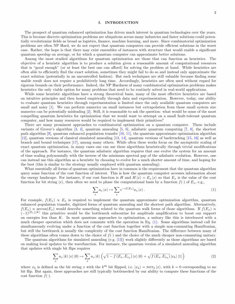
The prospect of quantum enhanced optimization has driven much interest in quantum technologies over the years.This is because discrete optimization problems are ubiquitous across many industries and faster solutions could poten-tially revolutionize fields as broad as logistics, finance, machine learning, and more. Since combinatorial optimizationproblems are often NP Hard, we do not expect that quantum computers can provide efficient solutions in the worstcase. Rather, the hope is that there may exist ensembles of instances with structure that would enable a significantquantum speedup on average, or for which a quantum computer can approximate better solutions.

Among the most studied algorithms for quantum optimization are those that can function as heuristics. Theobjective of a heuristic algorithm is to produce a solution given a reasonable amount of computational resourcesthat is “good enough” (or at least the best one can afford) for solving the problem at hand. While heuristics areoften able to efficiently find the exact solution, sometimes they might fail to do so and instead only approximate theexact solution (potentially in an uncontrolled fashion). But such techniques are still valuable because finding someusable result does not require a prohibitively long time. Accordingly, heuristics are often used without regard forrigorous bounds on their performance. Indeed, the NP Hardness of many combinatorial optimization problems makesheuristics the only viable option for many problems that need to be routinely solved in real-world applications.

While some heuristic algorithms have a strong theoretical basis, many of the most effective heuristics are basedon intuitive principles and then honed empirically through data and experimentation. However, today, our abilityto evaluate quantum heuristics through experimentation is limited since the only available quantum computers aresmall and noisy [1]. We can perform numerics on small instances but extrapolation from those small system sizenumerics can be potentially misleading [2]. Still, it is reasonable to ask the question: what would be some of the mostcompelling quantum heuristics for optimization that we would want to attempt on a small fault-tolerant quantumcomputer, and how many resources would be required to implement their primitives?

There are many prominent approaches to combinatorial optimization on a quantum computer. These includevariants of Grover’s algorithm [3, 4], quantum annealing [5, 6], adiabatic quantum computing [7, 8], the shortestpath algorithm [9], quantum enhanced population transfer [10, 11], the quantum approximate optimization algorithm[12], quantum versions of classical simulated annealing [13, 14], quantum versions of backtracking [15, 16] as well asbranch and bound techniques [17], among many others. While often these works focus on the asymptotic scaling ofexact quantum optimization, in many cases one can use these algorithms heuristically through trivial modificationsof the approach. For instance, the quantum adiabatic algorithm requires that one evolve the system for an amountof time scaling polynomially with the inverse of the minimum spectral gap of the adiabatic evolution. However, onecan instead use this algorithm as a heuristic by choosing to evolve for a much shorter amount of time, and hoping forthe best (this is similar to the strategy usually employed with quantum annealing).

What essentially all forms of quantum optimization have in common is the requirement that the quantum algorithmquery some function of the cost function of interest. This is how the quantum computer accesses information aboutthe energy landscape. For instance, if our cost function is H and H |x〉 = Ex |x〉 so that Ex is the value of the costfunction for bit string |x〉, then often we need to phase the computational basis by a function f(·) of Ex, e.g.,∑

x

ax |x〉 7→∑x

e−if(Ex)ax |x〉 . (1)

For example, f(Ex) ∝ Ex is required to implement the quantum approximate optimization algorithm, quantumenhanced population transfer, digitized forms of quantum annealing and the shortest path algorithm. Alternatively,f(Ex) ∝ arccos(Ex) would describe something related to the quantum walk forms of those algorithms. If f(Ex) ∝(−1)(Ex≤K) this primitive would be the bottleneck subroutine for amplitude amplification to boost our supporton energies less than K. In most quantum approaches to optimization, a unitary like this is interleaved with amuch cheaper operation which does not commute with the operation in Eq. (1). Some algorithms instead call forsimultaneously evolving under a function of the cost function together with a simple non-commuting Hamiltonian,but still the bottleneck is usually the complexity of the cost function Hamiltonian. The difference between many ofthese algorithms often comes down to the choice of f(·) and the choice of the much cheaper non-commuting unitary.

The quantum algorithms for simulated annealing (e.g. [13]) work slightly differently as those algorithms are basedon making local updates to the wavefunction. For instance, the quantum version of a simulated annealing algorithmthat updates with single bit flips requires∑

x

ax |k〉 |x〉 |0〉 7→∑x

ax |k〉(√

1− f (Ex, Exk) |x〉 |0〉+√f (Ex, Exk) |xk〉 |1〉

)(2)

where xk is defined as the bit string x with the kth bit flipped, i.e. |xk〉 = notk |x〉, with k = 0 corresponding to nobit flip. But again, these approaches are still typically bottlenecked by our ability to compute these functions of thecost function f(·).

4

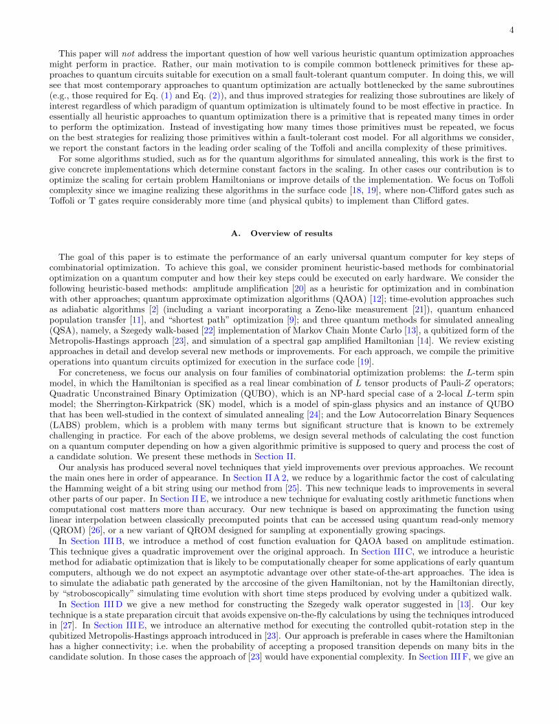
This paper will not address the important question of how well various heuristic quantum optimization approachesmight perform in practice. Rather, our main motivation to is compile common bottleneck primitives for these ap-proaches to quantum circuits suitable for execution on a small fault-tolerant quantum computer. In doing this, we willsee that most contemporary approaches to quantum optimization are actually bottlenecked by the same subroutines(e.g., those required for Eq. (1) and Eq. (2)), and thus improved strategies for realizing those subroutines are likely ofinterest regardless of which paradigm of quantum optimization is ultimately found to be most effective in practice. Inessentially all heuristic approaches to quantum optimization there is a primitive that is repeated many times in orderto perform the optimization. Instead of investigating how many times those primitives must be repeated, we focuson the best strategies for realizing those primitives within a fault-tolerant cost model. For all algorithms we consider,we report the constant factors in the leading order scaling of the Toffoli and ancilla complexity of these primitives.

For some algorithms studied, such as for the quantum algorithms for simulated annealing, this work is the first togive concrete implementations which determine constant factors in the scaling. In other cases our contribution is tooptimize the scaling for certain problem Hamiltonians or improve details of the implementation. We focus on Toffolicomplexity since we imagine realizing these algorithms in the surface code [18, 19], where non-Clifford gates such asToffoli or T gates require considerably more time (and physical qubits) to implement than Clifford gates.

A. Overview of results

The goal of this paper is to estimate the performance of an early universal quantum computer for key steps ofcombinatorial optimization. To achieve this goal, we consider prominent heuristic-based methods for combinatorialoptimization on a quantum computer and how their key steps could be executed on early hardware. We consider thefollowing heuristic-based methods: amplitude amplification [20] as a heuristic for optimization and in combinationwith other approaches; quantum approximate optimization algorithms (QAOA) [12]; time-evolution approaches suchas adiabatic algorithms [2] (including a variant incorporating a Zeno-like measurement [21]), quantum enhancedpopulation transfer [11], and “shortest path” optimization [9]; and three quantum methods for simulated annealing(QSA), namely, a Szegedy walk-based [22] implementation of Markov Chain Monte Carlo [13], a qubitized form of theMetropolis-Hastings approach [23], and simulation of a spectral gap amplified Hamiltonian [14]. We review existingapproaches in detail and develop several new methods or improvements. For each approach, we compile the primitiveoperations into quantum circuits optimized for execution in the surface code [19].

For concreteness, we focus our analysis on four families of combinatorial optimization problems: the L-term spinmodel, in which the Hamiltonian is specified as a real linear combination of L tensor products of Pauli-Z operators;Quadratic Unconstrained Binary Optimization (QUBO), which is an NP-hard special case of a 2-local L-term spinmodel; the Sherrington-Kirkpatrick (SK) model, which is a model of spin-glass physics and an instance of QUBOthat has been well-studied in the context of simulated annealing [24]; and the Low Autocorrelation Binary Sequences(LABS) problem, which is a problem with many terms but significant structure that is known to be extremelychallenging in practice. For each of the above problems, we design several methods of calculating the cost functionon a quantum computer depending on how a given algorithmic primitive is supposed to query and process the cost ofa candidate solution. We present these methods in Section II.

Our analysis has produced several novel techniques that yield improvements over previous approaches. We recountthe main ones here in order of appearance. In Section II A 2, we reduce by a logarithmic factor the cost of calculatingthe Hamming weight of a bit string using our method from [25]. This new technique leads to improvements in severalother parts of our paper. In Section II E, we introduce a new technique for evaluating costly arithmetic functions whencomputational cost matters more than accuracy. Our new technique is based on approximating the function usinglinear interpolation between classically precomputed points that can be accessed using quantum read-only memory(QROM) [26], or a new variant of QROM designed for sampling at exponentially growing spacings.

In Section III B, we introduce a method of cost function evaluation for QAOA based on amplitude estimation.This technique gives a quadratic improvement over the original approach. In Section III C, we introduce a heuristicmethod for adiabatic optimization that is likely to be computationally cheaper for some applications of early quantumcomputers, although we do not expect an asymptotic advantage over other state-of-the-art approaches. The idea isto simulate the adiabatic path generated by the arccosine of the given Hamiltonian, not by the Hamiltonian directly,by “stroboscopically” simulating time evolution with short time steps produced by evolving under a qubitized walk.

In Section III D we give a new method for constructing the Szegedy walk operator suggested in [13]. Our keytechnique is a state preparation circuit that avoids expensive on-the-fly calculations by using the techniques introducedin [27]. In Section III E, we introduce an alternative method for executing the controlled qubit-rotation step in thequbitized Metropolis-Hastings approach introduced in [23]. Our approach is preferable in cases where the Hamiltonianhas a higher connectivity; i.e. when the probability of accepting a proposed transition depends on many bits in thecandidate solution. In those cases the approach of [23] would have exponential complexity. In Section III F, we give an

5

Problem Algorithm Primitive(Table VIII and Table IX) (Table VII)

steps per day physical qubits Toffoli count

SK

Amplitude Amplification (§ III A) 4.8× 103 8.1× 105 2N2 +N +O(logN)

QAOA / 1st order Trotter (§ III B) 4.7× 103 8.6× 105 2N2 + 4N +O(1)

Hamiltonian Walk (§ III C) 3.3× 105 8.0× 105 6N +O(log2 N)

QSA / Qubitized (§ III E) 3.3× 105 8.4× 105 5N +O(logN)

QSA / Gap Amplification (§ III F) 3.9× 105 8.4× 105 5N +O(logN)

LABS

Amplitude Amplification (§ III A) 3.3× 103 8.0× 105 5N2/2 + 7N/2 +O(logN)

QAOA / 1st order Trotter (§ III B) 3.4× 103 8.4× 105 5N2/2 +O(N)

Hamiltonian Walk (§ III C) 4.9× 105 8.0× 105 4N +O(logN)

QSA / Qubitized (§ III E) 1.7× 103 8.8× 105 5N2+O(N)

QSA / Gap Amplification (§ III F) 1.7× 103 8.8× 105 5N2+O(N)

TABLE I. We compare the cost of implementing various types of heuristics optimization primitives in a fault-toleration costmodel. For concreteness, we give results for two problems: the Sherrington-Kirkpatrick model (SK) and Low AutocorrelationBinary Sequences problem (LABS). The numerical values from Table VIII and Table IX are based on a problem size of N = 256,a surface code cycle time of 1 µs, and a physical gate error rate of 10−3 (there are other assumptions as well, covered in moredetail in Section IV). Note that depending how they would be used, it might be appropriate to scale the Hamiltonian walksteps by a factor of λ which is roughly λSK ≈ N2/2 and λLABS ≈ N3/3. We simplify the complexity scaling estimates fromTable VII by treating as constant the bits of precision for numerical values.

explicit LCU-based oracle for the spectral gap amplified Hamiltonian introduced in [14]. This explicit oracle enablesa cost analysis of the approach, which we provide. Apart from assisting with our goal of estimating early quantumcomputer performance, many of these innovations produce asymptotic improvements to the approaches we consider.

Having compiled the primitive operations of our chosen approaches and established how to query cost functionsfor our chosen problems, we are able to numerically estimate the computational resources needed to execute theseprimitives on a quantum computer. Based on our assumption that the quantum computer will be built from super-conducting qubits and employ the surface code to protect the computation from errors, we focus on minimizing thenumber of ancilla qubits and non-Clifford gates that would be required. This approach is founded on the knowledgethat non-Clifford operations are significantly harder than Clifford operations to perform in the surface code.

We give an example of some of our ultimate findings in Table I. In the table we provide the leading order scalingof the number of Toffoli gates needed to perform an update using five of the heuristics that we consider for twobenchmark problems – LABS and SK. These scalings are reproduced from Table VII and presented in a simplifiedform where we assume that the working precision for various calculations is a constant. We also reproduce key figuresfrom Table VIII and Table IX to show how we expect these estimated complexity scalings translate into the runtimeof an early quantum computer. In Table I we show the estimated number of steps of the chosen algorithmic primitivethat could be executed in a single day on a quantum computer for a problem size of N = 256, a relatively smallproblem size that would be reasonable to execute with only a single Toffoli factory as we assume in Table VIII andTable IX. We also present the estimated number of physical qubits needed.

We find that, despite great efforts made to optimize our compiled quantum circuits, the costs involved in imple-menting heuristics for combinatorial optimization will be taxing for early quantum computers. Not surprisingly, toimplement problems between N = 64 and N = 1024 we find that hundreds of thousands of physical qubits are requiredwhen physical gate error rates are on the order of 10−4 and sometimes over a million are required for physical gateerror rates on the order of 10−3. But even more concerning is that the number of updates that we can achieve in aday (given realistic cycle times for the error correcting codes) is relatively low, on the order of about ten thousandupdates for the smallest instances considered of the cheapest cost functions. With such overheads, these heuristicswould need to yield dramatically better improvements in the objective function per step than classical optimizationheuristics. From this we conclude that, barring significant advances in the implementation of the surface code (e.g.,much faster state distillation), quantum optimization algorithms offering only a quadratic speedup are unlikely toproduce any quantum advantage on the first few generations of superconducting qubit surface code processors.

B. Organization of paper

Our paper is divided into essentially two parts. In the first part (Section II) we introduce and provide explicitcompilations for a wide variety of subroutine or “oracle” circuits which perform operations related to specific problem

6

Hamiltonians. In the second part of our paper (Section III) we describe a variety of heuristic algorithms for quantumoptimization and discuss how the oracle circuits of Section II can be called in order to implement these algorithms.We will see that the same “oracle” circuits are required by many algorithms. The results of Section III essentiallyprovide query complexities to implement the primitives of common quantum optimization heuristics with respect tothe oracles of Section II. Thus, while the results of Section II are adapted to particular problem Hamiltonians, theresults of Section III are fairly general. We now describe our results in slightly more detail.

Section II details strategies for realizing five straightforward oracle circuits which are detailed therein for each of fourproblem Hamiltonians in Table III. The specific problems we focus on are introduced at the beginning of Section II.These five oracles correspond to: (Section II A) the direct computation of a cost function into a quantum register,(Section II B) the computation of the difference between the cost of two computational basis states which differ by aspecific single bit, (Section II C) an operation which phases the computational basis by an amount proportional to thecost, (Section II D) the realization of a qubitized quantum walk [28] which encodes eigenvalues of the cost function,and (Section II E) the computation of arithmetic functions of an input value using QROM [26]. Our approach tocomputing arithmetic operations using QROM is likely useful in other contexts and is a new technique from this work.The culmination of Section II is Table IV which gives leading order constants in the scaling of Toffoli, T and ancillacomplexities for all five of these oracles and for all four of the problems. Even though the first two cost functions weintroduce in Section II have fairly general specifications, they do not capture exploitable structure in all optimizationproblems of interest. Still, we imagine that the motifs developed in Section II will be helpful for any future workseeking to develop similar circuits for other cost functions.

Section III describes how the oracle circuits of Section II are queried in order to realize the essential primitivesof many fault-tolerant quantum heuristics for optimization. This section contains a mixture of new results and areview of established methods. Section III A reviews how one can use amplitude amplification [20] heuristically foroptimization and also discusses how and why one might combine amplitude amplification with other algorithms inthis section. Section III B discusses strategies for executing QAOA [12] within fault-tolerant cost models. While mostof this section is review, we also discuss the combination of QAOA with amplitude amplification based methods formore efficiently extracting the cost function value.

Section III C discusses several approaches to quantum optimization that are based on time evolution or quantumwalks generated by a cost function and simple driver. First, we review the adiabatic algorithm [2] and well knownmethods for how it might be digitized using product formula type circuits. We then introduce a method of simulatingthe adiabatic algorithm based on qubitized quantum walks. Next, we review how the adiabatic algorithm can becombined with a Zeno-like measurement approach which corresponds to evolution under static Hamiltonians forrandom durations [21], and give some new results about how to optimally choose the distribution of those durations.

The remainder of Section III focuses on three approaches to a quantum algorithm which accelerates classicalsimulated annealing. In terms of implementation, these are the most complex algorithms studied in the paper.For the three variants of the quantum simulated annealing algorithms, we provide the first complete compilation ofcircuits which execute the heuristic primitive. In Section III D we analyze and compile the original version [13] ofthese algorithms that is based on Szegedy quantum walks [22]. As anticipated, this approach is the least efficient ofthe three studied. In Section III E we focus on what is essentially a qubitized version of the Szegedy quantum walk.The primary characteristics of this approach were independently described in [23] (a paper that came out during thepreparation of our own) but we go beyond that work to determine (and in some ways improve upon) constant factorsin the scaling. Finally, in Section III F we compile the algorithm for quantum simulated annealing based on spectralgap amplification [29], using an improvement based on qubitization. The results of Section III are summarized inTable VI and Table VII, which give the query complexities with respect to the oracles of Section II and overall gateand ancilla complexities of all algorithms of Section III for all of the cost functions of Section II.

Finally, we conclude in Section IV with a discussion of these results. Our discussion includes an attempt tocontextualize the ultimate cost of these heuristic primitives by giving the Toffoli count, ancilla count, and totalnumber of physical qubits and wallclock time that would be required to realize these primitives given various resourcebudgets and assumptions in the surface code. These concrete resource estimates are given in Table VIII and Table IX.We then finish with a discussion of how these results lead to a fairly pessimistic outlook on the viability of obtainingquantum advantage for optimization by using a small quantum computer unless one is able to obtain significantlybetter than a quadratic speedup over classical alternatives.

II. ORACLES AND CIRCUIT PRIMITIVES FOR SPECIFIC COST FUNCTIONS

While many paradigms of quantum optimization require the same bottleneck subroutines for their implementation,aspects of these subroutines will always be specific to the particular problem that one intends to optimize. Thus, inorder to give concrete implementations and develop a sense of how many resources would be required for steps of

7

common quantum heuristics, aspects of our work are adapted to particular problem Hamiltonians (equivalently here,“cost functions”) of interest. There are four main types of Hamiltonians that we consider in this paper.

The first two types of Hamiltonians we will study are of interest because they are programmable instances ofoptimization problems that one might encounter in practical situations. The second two types of problems we willstudy are of interest more to those who study statistical physics and for different reasons: because they defineensembles of instances for which the average case has known and interesting properties. While solutions to specificinstances of the latter two problems are probably not of much value, we anticipate they will be interesting problemson which to investigate the performance of a quantum computer. The four problems we study are described below.

1. L-term spin model: The most general Hamiltonian we will consider is the one we will refer to simply as the“L-term spin model”. This Hamiltonian is a linear combination of L tensor products of Pauli-Z operators,

HL =

L∑`=1

w`∏i∈q`

Zi, (3)

where w` are real scalars, Zi is the Pauli-Z operator on qubit i, N is the number of qubits in the cost function,and q` is a unique set of up to N integers which also take values between 1 and N (it is a set of integerscorresponding to the indices of qubits on which term ` acts). One might anticipate that it would be helpful toalso specify this Hamiltonian in terms of its many-body order k = max|q`|. However, perhaps surprisingly,none of the algorithms discussed in this paper have a Toffoli complexity that scales explicitly in k.

2. Quadratic Unconstrained Binary Optimization: We will also consider an NP-Hard example of HN2/2

known as Quadratic Unconstrained Binary Optimization (QUBO). The QUBO Hamiltonian is expressed as

HQUBO =∑i≤j

wij

(11− Zi

2

)(11− Zj

2

)=∑i<j

JijZiZj +∑i

hiZi +K (4)

where K is a constant term that we will ignore from this point forward as this never needs to be explicitlysimulated or computed for the purposes of optimizing the model, and the coefficients Jij and hi can be computedfrom the wij . This form of the model is also known as the Ising model but we refer to it here as QUBO sincethe Ising model can also mean a model with more limited connectivity and regular coefficients in some contexts.

3. Sherrington-Kirkpatrick: This problem corresponds to a widely studied model of spin glass physics [24].The Sherrington-Kirkpatrick (SK) model is an example of the following QUBO Hamiltonian:

HSK =∑i<j

wijZiZj , wij ∈ −1, 1 , ‖HSK‖ ≤ N2/2, (5)

and the values of wij are usually chosen at random. The SK model is the focus of many studies on heuristicoptimization, especially ones focusing on variants of simulated annealing. There is also a variant of the SKmodel which has the same statistical properties where the coefficients are Gaussian distributed real numbers.

4. Low Autocorrelation Binary Sequences: We think it would be interesting to use a quantum computer toattempt to optimize problems that are very challenging on average. One problem is the Low AutocorrelationBinary Sequences (LABS) problem, also known as the Bernasconi model in physics [30]:

HLABS =

N−1∑k=0

H2k Hk =

N−k∑i=1

ZiZi+k, ‖HLABS‖ ≈ N3/3, (6)

which is an instance of HN3 . This model is known to be extremely difficult; in fact the best classical algorithmhas scaling like Θ(1.73N ) and has only been run for problem sizes up to N = 66 [31]. However, we note that themodel is not really a “problem” in the usual computer science sense because there is only one instance definedfor each problem size. A variant of the LABS problem that we will consider is when the squared operators areinstead replaced with absolute values, as one can verify that the ordering of the low energy solutions would beunchanged by this modification, and it is sometimes less expensive to simulate with a quantum computer.

The remainder of Section II discusses concrete circuit realizations for “oracles” which provide information aboutthese cost functions of interest. Here we slightly abuse the term “oracle” to mean a circuit primitive which is repeatedlyqueried throughout an algorithm, usually revealing information about the problem we are solving. These oracles are

8

symbol meaning

x bitstring corresponding to a candidate solution of the optimization problem

N number of bits needed to specify a candidate solution

Ex cost (a.k.a. energy) of candidate solution x as specified by a cost function

Hcf Hamiltonian operator corresponding to a cost function “cf”

b number of bits used to specify the precision of an oracle

L number of terms in a spin model (type of cost function)

λ the normalization parameter for LCU methods, related to the Hamiltonian 1-norm

β inverse temperature in simulated annealing

C Toffoli or T cost of some oracle

A ancilla required to implement some oracle that must be kept

B temporary ancilla required to implement some oracle

TABLE II. A list of common symbols we use throughout this paper.

oracle oracle definition precision definition

Odirect Odirect∑x ψx |x〉 |0〉

⊗bdir 7→∑x ψx |x〉 |Ex〉

∣∣∣Ex − Ex∣∣∣ ≤ 2−bdir maxx |Ex|

Odiffk Odiff

k

∑x ψx |x〉 |0〉

⊗bdif 7→∑x ψx |x〉 |δE

(k)

x 〉 , |y〉 = Xk |x〉∣∣∣δE(k)

x − Ex + Ey

∣∣∣ ≤ 2−bdif maxx,y |Ex − Ey|

Ophase(γ) Ophase(γ)∑x ψx |x〉 7→

∑x e−iγExψx |x〉

∣∣∣γEx − γEx∣∣∣ ≤ 2−bpha

OLCU 〈0|⊗ logLOLCU |0〉⊗ logL = H/λ, H =∑L`=1 w`U`, λ =

∑L`=1 |w`|

∣∣√w` −√w`∣∣ ≤ 2−bLCU

Ofunβ Ofun

β |z〉 |0〉⊗bsm 7→ |x〉 |f(βz)〉∣∣∣f(βz)− f(βz)

∣∣∣ ≤ 2−bfun

TABLE III. Quick definitions of the most important “oracle” circuits discussed in this work. Here, we slightly abuse theterm “oracle” to mean a circuit primitive which is repeatedly queried throughout an algorithm, usually revealing informationabout the problem we are solving. Throughout the paper we will use C to denote Toffoli (or occasionally T) complexity whileA and B will denote persistent and temporary ancilla costs, respectively. For some of these oracles there are different Toffolicosts when performing them in the forward and reverse directions. We always pair a forward oracle with a reverse oracle, sowill give the average cost. In some cases the computation may introduce ancilla qubits not shown here, that are erased inthe inverse computation. For the function evaluation oracle we incorporate multiplication by the inverse temperature β. Theapproximation f is given to bsm bits, but for generality we allow an error 2−bfun which may be larger than 2−bsm .

used by multiple algorithms throughout our paper. In Section II A, we explain how to implement cost function oraclesthat are required to return the cost of a specific candidate solution x. We refer to such oracles as “direct energyoracles”. In Section II B, we explain how to implement cost function oracles that are required to return the differencein cost between two candidate solutions that differ by exactly one bit. In Section II C, we explain how to implementcost function oracles that are required to return the cost function as a phase, rather than as a value written to aseparate quantum register. In Section II D, we explain how to implement cost function oracles that are required toimplement the cost function as a direct application of the Hamiltonian onto a target quantum register. Finally, inSection II E, we consider the cost of evaluating functions whose input is the difference in cost of candidate solutionsas described in the other parts of this section.

We summarize the content of this section using three tables. In Table II we give a list of the symbols we use forreporting our computational complexity results. This table aids in the interpretation of the following two tables. InTable III, we summarize the definitions of the various different kinds of oracles considered in this section. Finally, inTable IV, we summarize the complexities of each of the sixteen cost function oracles (four types of oracles for eachof four types of cost functions) as well as the complexity of calculating functions of those oracle outputs. In thesetables, and throughout the paper, we use log to indicate logarithms base 2.

A. Oracles for direct cost function evaluation

Many of the algorithms considered in this work are formulated in terms of a query to an oracle which computes thevalue of the cost function C (for instance, one of the Hamiltonians discussed above) in a binary register. For instance,

9

cost function oracle type Toffoli (*or T) gate count C persistent ancilla A temporary ancilla BL-term Spin Model direct energy L bdir (8) bdir (9) bdir − 1 (10)

HL energy difference 2L bdif +O(1) (8) bdif (9) bdif − 1 (10)

direct phase* 1.15L(bpha + logL) +O(logL) (36) 0 (37) 1 (38)

Hamiltonian walk 3L+ 2 bLCU +O(logL) (56) 2 logL+ 2 bLCU +O(1) (57) logL+O(1) (58)

Quadratic direct energy N2bdir/2 +O(Nbdir) (11) bdir (12) bdir − 1 (13)

Unconstrained energy difference N bdif (25) bdif (26) bdif − 1 (27)

Binary Optimization direct phase* 0.575N2(bpha + 2 logN) +O(N2) (39) 0 (40) 1 (41)

HQUBO Hamiltonian walk N(bLCU + 2 logN) +O(N) (73) 2bLCU + 4 logN +O(1) (75) 3 logN +O(log bLCU) (76)

Sherrington- direct energy N2 (16) 2 logN (17) 4 logN (18)

Kirkpatrick Model energy difference 2N (28) logN + 1 (29) 2 logN +O(1) (30)

HSK direct phase 2N2 + b2pha/2 +O(bpha log bpha) (42) 2 logN + bpha +O(log bpha) (43) 4 logN (44)

Hamiltonian walk 6N +O(log2 N) (82) 2 logN +O(1) (83) 3 logN +O(1) (84)

Low direct energy 5N(N + 1)/4 (20) 2 logN + 1 (21) 3 logN + 3 (22)

Autocorrelation energy difference 5N(N + 1)/2 (20) 2 logN + 1 (21) 3 logN + 3 (22)

Binary Sequences direct phase 85N2 + min

(12Nb2pha,

910N2)

+O(Nbpha log bpha) (49) bpha +O(log bpha) (46) 5 logN +O(log bpha) (50)

HLABS Hamiltonian walk 4N +O(logN) (87) 3 logN +O(1) (88) 2 logN +O(1) (89)

function evaluation b2sm + bdif +O(bsm log bsm + 2bfun/2) (95) 2bsm +O(log bsm) (97) bdif − 1 (98)

arcsine evaluation (bsm + bfun)2 + bdif +O(bsm log bsm + 2bfun/2) (96) 2bsm + bfun +O(log bsm) (99) bdif − 1 (100)

TABLE IV. Summary of complexities for realizing oracles used throughout this paper. Next to the complexity entry is anumber indicating the equation in the paper which gives the full expression in context. The energy difference for HL and LABSjust has twice the Toffoli cost and the same ancilla cost as the direct energy oracle, because it is found by evaluating the energytwice. These oracles and the meaning of their precision parameters b are defined in Table III. The Toffoli count is reportedexcept when the oracle type for that cost function is marked with (*), which indicates that T count is reported instead. Herewe include only the main terms in the order expressions. We use these costings to determine the complexities in Table VII.

if we have a wavefunction |ψ〉 =∑x ψx |x〉 where the computational basis states |x〉 are eigenstates of C such that

C |x〉 = Ex |x〉 then we define the direct energy evaluation oracle Odirect as a circuit which acts as

Odirect∑x

ψx |x〉 |0〉⊗bdir 7→∑x

ψx |x〉 |Ex〉 (7)

where Ex is a binary approximation to Ex using bdir bits. We provide some strategies for how to realize this oracle forspecific problems with low Toffoli complexity. We will refer to the Toffoli complexity of this oracle as Cdirect. However,first we will discuss an efficient method for performing reversible in-place addition of a constant. This routine will becritical to our implementation.

1. Direct energy oracle for L-term spin model and QUBO

We will now explain how to implement the direct energy oracle for the HL Hamiltonian with low Toffoli complexity.We will represent the energy Ex in the two’s complement binary representation, as this encoding enables efficientmethods for addition [32]. In two’s complement positive integers have a normal binary representation whereas negativeintegers are the complement of that representation minus one. For instance, in 4-bit two’s complement 310 = 00112

whereas −310 = 11002 + 1 = 11012. Zero still corresponds to all bits zero. The fact that we need to add one fornegative numbers complicates our approach but this representation is still preferable for our purposes.

The main idea behind our approach will be to add or subtract the value of each term’s coefficient w` to a b-bitoutput register based on the parity of the string

∏i∈q` Zi. To perform addition or subtraction controlled on a qubit,

we use the fact that one can switch between addition and subtraction by applying not gates to the target register intwo’s complement representation. That is, applying not gates to all qubits of a register will change |v〉 to |−v − 1〉.Adding w to this register will give |w − v − 1〉, then applying not gates to all qubits again will yield |v − w〉. Toperform addition or subtraction controlled on a qubit, one can use the procedure shown in Figure 4(a) of [32] (seeAppendix D 2). The complete procedure to compute the energy is then as given in Algorithm 1.

10

Algorithm 1 Energy evaluation for L-term spin model and QUBO

Require: A quantum state∑x ax |x〉, a vector of weights w` that specifies the L-term spin model or QUBO Hamiltonian.

Ensure: An output state of the form∑x ax |x〉 |Ex〉, where H is the relevant Hamiltonian and Ex is the approximate eigenvalue

of H corresponding to |x〉.1: Use Clifford gates (cnot gates) to compute the parity of the term

∏i∈q`

Zi in-place in a single system qubit |π`〉. Specifically,

if xi is the ith bit of computational basis state x then we are using cnots to compute π` = (∑i∈q`

xi) mod 2.

2: Controlled on |π`〉, use more cnot gates to negate every bit of the output register. We will refer to this output register as|v〉. Thus, after this step we will have the state |0〉 |v〉 if the first bit holds π` = 0 and we will have the state |1〉 |−v − 1〉 ifthe first bit holds π` = 1.

3: Using the strategy described in Appendix D 2 for the addition of a constant, add a bdir-bit binary approximation w` to thecoefficient w` into the output register. This step has Toffoli complexity bdir− 2 where bdir is the size of the output register.After this step we will have the state |0〉 |v + w`〉 if π` = 0 and we will have the state |1〉 |w` − v − 1〉 if π` = 1.

4: Negate the output register using cnot gates, controlled on |π`〉. After this step we will have the state |0〉 |v + w`〉 if π` = 0and we will have the state |1〉 |v − w`〉 if π` = 1.

5: Using Clifford gates uncompute the parity π`.

After performing this for L terms one can verify that this will produce the intended state |v〉 = |Ex〉 in the outputregister. Toffoli gates enter only through the adder in step 3. Thus, in total our approach has Toffoli complexityCdirectL and ancilla requirements Adirect

L ,BdirectL given by

CdirectL = L (bdir − 2) < Lbdir, (8)

AdirectL = bdir, (9)

BdirectL = bdir − 1 < bdir, (10)

where the ancilla refer to the carry bits for the adder in addition to the bdir bits required to output the energy. Wenote that for this oracle these costs have no dependence on the many-body order of the Hamiltonian HL since thisonly affects the number of cnot gates used to compute the parity of the terms.

This exact same reasoning can be used to determine the complexity of computing the energies for the QUBOHamiltonian. Due to the relative lack of structure in QUBO, there is no obvious way to improve over this generalcomplexity. There we have L = N(N + 1)/2 terms and so from Eq. (8), Eq. (9) and Eq. (10) we require a number ofToffolis and ancillas equal to

CdirectQUBO =

N2bdir

2+Nbdir

2−N(N + 1) =

N2bdir

2+O(Nbdir), (11)

AdirectQUBO = bdir, (12)

BdirectQUBO = bdir − 1 < bdir. (13)

2. Direct energy oracle for SK model

Here we show that the energy for the SK model can be computed with only N2 Toffolis and a logarithmic numberof ancillas. The method we use is a sum of tree sums of bits. It is also possible to just use a tree sum with a Toffolicost of about N2/4, but the drawback is that this method would need N2/2 ancilla qubits, which is prohibitive.

For the SK model it is convenient to replace −1 with 0, so the sum takes values between 0 and L. That correspondsto dividing the Hamiltonian by 2 and shifting it, which does not change the optimization problem, but means we areonly summing bits. If we were to sum the bits in the obvious way, the Toffoli complexity would be approximatelyN2 logN . However, we can take advantage of the fact we are summing bits to reduce the complexity to O

(N2).

Our methods are based on tree sums of bits. In [25] it was shown that it is possible to sum L bits using L−1 Toffoligates and L− 1 ancilla qubits, and this sum can be uncomputed with no Toffoli cost. As discussed in [25], it is alsopossible to perform sums in approaches that reduce the number of ancilla at the price of increasing the number ofToffoli gates. In particular, we can subdivide the bits we are summing into about L/ logL groups of size logL, startby using the tree sum approach to sum each of the groups, add it into a running sum, and uncompute it. The numberof ancillas needed is reduced to approximately logL for each of the tree sums. There is also a cost of approximatelyL for adding the tree sums, giving a total complexity of approximately 2L.

To be more specific, taking into account that L need not be a power of two, we can use M = dL/dlogLee − 1groups of size dlogLe, except for a remaining group of size J ≤ dlogLe such that MdlogLe + J = L. That is, there

11

are dL/dlogLee groups, and J can be smaller than dlogLe. The Toffoli cost of computing each of these sums is

MdlogLe −M + J − 1 = L−M − 1 = L− dL/dlogLee. (14)

The cost of the additions is

M∑j=1

[dlog(J + jdlogLe+ 1)e − 1] ≤M(dlog(L+ 1)e − 1)

≤MdlogLe< (L/dlogLe)dlogLe = L. (15)

We have assumed that L > 1 and hence logL > 0. The first line of Eq. (15) comes from starting with the sum over Jbits and then adding each of the sums over dlogLe to it. After adding j of the sums over dlogLe bits, the maximumvalue of the sum is J + jdlogLe, so the number of bits needed to store the result is dlog(J + jdlogLe+ 1)e, and thenumber of Toffolis needed for that sum is one less than that. The inequality in the first line comes from the fact thatthe total number is never less than L, so the cost of the additions is never greater than dlog(L+ 1)e−1. The inequalityin the second line is because dlog(L+ 1)e − 1 ≤ logL. The inequality in the third line is using M < L/dlogLe.

Therefore, the total Toffoli cost is less than 2L. The ancilla cost of each tree sum is dlogLe−1, there are dlog(L+ 1)eancilla needed for the total, and dlog(L+ 1)e − 1 temporary ancillas for the addition of the tree sum into the total.Since the ancillas in the tree sum are uncomputed, they contribute to an overall temporary ancilla cost, meaning thetemporary ancilla cost is 2 logL+O(1) and the persistent ancilla cost (for the total) is logL+O(1).

Since L = N(N −1)/2, if we were to use a tree sum the cost would be less than N2/2, but the ancilla cost would beapproximately N2/2. The sum could be uncomputed without ancillas, giving an average (compute and uncompute)cost of N2/4. We expect that the tradeoff is not worth it in this case. However, by using the sum of tree sums, weget a Toffoli cost less than N2, and an ancilla cost that is logarithmic in N . That gives costs for the SK model of

CdirectSK < N2, (16)

AdirectSK ≤ 2 logN, (17)

BdirectSK < 4 logN. (18)

3. Direct energy oracle for LABS model

Next we show that for the LABS problem it is possible to compute the energy with a Toffoli cost of 5N(N + 1)/4for N ≥ 64, with a logarithmic number of ancilla qubits. We improve over the application of our general techniqueby specializing the implementation to the LABS problem. Since the LABS problem has L = O(N3) with maximuminteger energy values of O(N3), we would expect a complexity of O(N3). Instead, we show that it is possible toperform the direct energy evaluation at cost O(N2). We focus on the form of the LABS Hamiltonian that is expressed

as∑Nk=1 |Hk| where Hk is as defined in Eq. (6) (as we mentioned, this form of the problem has the same ordering of

the low energy landscape).In the following we use Ek to denote the eigenvalue of Hk. It will be most efficient to use the sum of tree sums

approach described above. Here we need to find Ek by using +1 and −1 rather than +1 and 0, because we need totake the absolute value, so we need an extra bit for the sign. Therefore, after summing bits, we will need to multiplyby 2 (which has no Toffoli cost), followed by subtracting the number of bits. The overall approach is then as follows.We will sum k starting at k = N − 1 and go down to zero, so the number of bits at each step is minimized. For eachvalue of k we will perform Algorithm 2.

Algorithm 2 Energy evaluation for LABS model

Require: A quantum state∑x ax |x〉, the set of all terms in the LABS Hamiltonian Hk.

Ensure: An output state of the form∑x ax |x〉 |Ex〉.

1: Compute for computational basis vector |x〉 the value of Ek in a scratch register |u〉 that will require dlog(N − k + 1)e+ 1ancilla to store (with +1 for the sign).

2: Controlled by the highest bit of u (the sign bit in two’s complement), use cnot gates to negate the value of the outputregister |v〉. At this point we have |u〉 |v〉 if u ≥ 0 or |u〉 |−v − 1〉 if u < 0.

3: Add the scratch register into the output register.4: Use cnots to negate the output register controlled on the highest bit of the |u〉 register.5: Uncompute |u〉.

12

In Step 1, the Toffoli complexity computing each Ek is approximately 2(N − k) plus the cost of subtracting N − k.In two’s complement we can determine whether the number is negative or positive by looking at the highest bit;if the highest bit is 1 then we know the value is negative. This justifies the operations in Step 2. Since Step 2requires no non-Clifford operations, it can be neglected in our cost analysis. In Step 3, the state is |u〉 |u+ v〉 ifu ≥ 0 or |u〉 |v − u〉 if u < 0; equivalently we now have the state |u〉 |v + |u|〉. The output register will be of sizedlog[(N − k)(N − k + 1)/2 + 1]e+ 1 so the Toffoli cost is dlog[(N − k)(N − k + 1)/2 + 1]e.

The output register is significantly larger than the scratch register. However, with a slight modification of theprocedure in Appendix D 2 we can allow this register to be smaller with no additional Toffoli cost. First, considerexpanding the number of qubits |u〉 is encoded on. This is of course trivial for positive numbers. For negative u,for n bits it is encoded as 2n + u. Therefore, if we have a number that is negative and we need to map it to anegative number on some larger number of bits n′, then we need to map 2n + u to 2n

′+ u, which means adding

2n′ − 2n =

∑n′−1j=n 2j . This means that bits n+ 1 to n′ of the negative number encoded on the n′ bits need to be ones.

These can be set by using CNOTs controlled by bit n, which means no additional Toffoli cost is needed to encode thenumber into more qubits. A further simplification can be used to eliminate the need for those extra qubits. First,rearrange the addition circuit as in Figure 18 so that the qubits of |u〉 are only used as controls and not changed.Since all of the additional qubits for |u〉 contain the same value as the sign qubit of |u〉, we may use that sign qubitas the control instead of any of those additional qubits. Then the additional qubits are not used, and can be omitted.

There is an improvement that we can make when we take into account that each computation needs to be pairedwith an uncomputation. This is because, in step 5, if we are computing an energy that we will later uncompute, thenwe can use the strategy of [32] to erase |u〉 using X measurements and no Toffoli cost. A phase correction is required,but that can be done when we later uncompute the LABS energy. This means that in step 5 we have a cost of N − kin uncomputing the LABS energy, but no Toffoli cost in computing the LABS energy. Because each computationis paired with an uncomputation, it is therefore convenient to give the average complexity of N − k. The largesttemporary ancilla cost is when we need to uncompute the overall Hamiltonian, when it is 2 log(N − k) +O(1). Thatis still less than the temporary ancilla cost in step 3, so can be ignored.

After repeating this for the N values of k one can verify that the output register will contain the energy of theLABS Hamiltonian. Toffoli gates enter only through steps 1, 3 and 5. The primary contribution to the complexity isthe computation of Ek in steps 1 and 5. Ignoring the complexity of subtracting N − k, the Toffoli complexity is

N−1∑k=0

3(N − k) = 3N(N + 1)/2. (19)

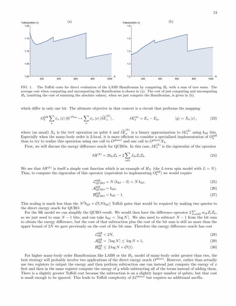
The cost of the subtractions as well as the additions in step 3 will increase the cost, but also 2(N−k) is an overestimateof the cost of adding n − k bits. In particular, we can use tree sums of as many as approximately logN bits, ratherthan just log(N − k), with no penalty in terms of the temporary ancilla cost. The computed costs are shown inFigure 1(a), and it is found for the range of N we are interested in (64 – 1024), the constant factor on N(N + 1) isless than 1.2, rather than 1.5 (in fact, this bound is good for N ≥ 45). In particular, the constant factors for N = 64,128, 256 and 1024 are 1.16466, 1.12673, 1.13945, and 1.0901, respectively. To simplify the expressions we give theslightly looser bound in the table

CdirectLABS < 5N(N + 1)/4, (20)

with the caveat that it is for N ≥ 45. The number of ancilla we will require is

AdirectLABS = dlog[N(N + 1)/2 + 1]e ≤ 2 logN + 1, (21)

BdirectLABS = dlog[N(N + 1)/2 + 1]e+ dlog(N − k + 1)e+ 2 ≤ 3 logN + 3. (22)

The persistent ancilla are for the output value. Approximately 2 logN of the temporary ancilla are for carry bits inthe addition and logN are for the scratch register. We assume N > 1 for the inequalities which omits the trivial case.This example illustrates how taking advantage of problem structure can lead to advantages over the implementationof an oracle intended to handle a more general case.

B. Energy difference oracles

For some of the algorithms discussed in this work (specifically the quantum versions of simulated annealing) weoften need the direct energy oracle only as means to compute a difference between the energies of two different states

13

200 400 600 800 1000N1.00

1.05

1.10

1.15

1.20Toffolis/(N(N+1))

200 400 600 800 1000N1.2

1.3

1.4

1.5

1.6Toffolis/(N(N+1))(a) (b)

FIG. 1. The Toffoli costs for direct evaluation of the LABS Hamiltonian by computing Hk with a sum of tree sums. Theaverage cost when computing and uncomputing the Hamiltonian is shown in (a). The cost of just computing and uncomputingHk (omitting the cost of summing the absolute values), when we just compute the Hamiltonian, is given in (b).

which differ in only one bit. The ultimate objective in that context is a circuit that performs the mapping

Odiffk

∑x

ψx |x〉 |0〉⊗bdif 7→∑x

ψx |x〉 |δE(k)

x 〉 , δE(k)x = Ex − Ey, |y〉 = Xk |x〉 , (23)

where (as usual) Xk is the not operation on qubit k and δE(k)

x is a binary approximation to δE(k)x using bdif bits.

Especially when the many-body order is 2-local, it is more efficient to consider a specialized implementation of Odiffk

than to try to realize this operation using one call to Odirect and one call to OdirectXk.

First, we will discuss the energy difference oracle for QUBOs. In this case, δE(k)x is the eigenvalue of the operator

δH(k) = 2hkZk + 2∑i6=k

JikZiZk. (24)

We see that δH(k) is itself a simple cost function which is an example of HN (the L-term spin model with L = N).Thus, to compute the eigenvalue of this operator (equivalent to implementing Odiff

k ) we would require

CdiffQUBO = N (bdif − 2) < N bdif , (25)

AdiffQUBO = bdif , (26)

BdiffQUBO = bdif − 1. (27)

This scaling is much less than the N2bdif +O(Nbdif) Toffoli gates that would be required by making two queries tothe direct energy oracle for QUBO.

For the SK model we can simplify the QUBO result. We would then have the difference operator 2∑i 6=k wikZiZk,

so we just need to sum N − 1 bits, and can take bdif = dlogNe. We also need to subtract N − 1 from the bit sumto obtain the energy difference, but the cost of that subtraction plus the cost of the bit sum is still no more than theupper bound of 2N we gave previously on the cost of the bit sum. Therefore the energy difference oracle has cost

CdiffSK < 2N, (28)

AdiffSK = dlogNe ≤ logN + 1, (29)

BdiffSK ≤ 2 logN +O(1). (30)

For higher many-body order Hamiltonians like LABS or the HL model of many-body order greater than two, thebest strategy will probably involve two applications of the direct energy oracle Odirect. However, rather than actuallyuse two registers to output the energy and then perform subtraction one can instead just compute the energy of xfirst and then in the same register compute the energy of y while subtracting all of the terms instead of adding them.There is a slightly greater Toffoli cost because the subtraction is on a slightly larger number of qubits, but that costis small enough to be ignored. This leads to Toffoli complexity of 2 Cdirect but requires no additional ancilla.

14

C. Oracles for phasing by cost function

In some contexts our goal will be to phase each computational state on which the wavefunction has support by anamount proportional to the energy of that computational basis state (this task is equivalent to performing evolutionunder a diagonal Hamiltonian for unit time). We will refer to circuits that achieve this task as a “phase” oracle anddefine them to act as

Ophase(γ)∑x

ψx |x〉 7→∑x

e−iγExψx |x〉∣∣∣γEx − γEx∣∣∣ ≤ 2−bpha . (31)

To simplify the following discussion, we assume that Ex is shifted such that it is non-negative. Such a shift correspondsto an unobservable global phase.

To realize this oracle, one strategy would be to first approximately compute Ex into a register using Odirect, thenmultiply by γ and perform further logic to phase the system by the amount in the register. For instance,(

Odirect)† (

11⊗ Uphase (γ))Odirect

∑x

ψx |x〉 7→∑x

e−iγExψx |x〉 (32)

where the phasing operation needed is

Uphase (γ) =

2bdir−1∑k=0

exp

(2πikγ

2bdir

)|k〉〈k| . (33)

The value of 2πkγ/2bdir would correspond to the approximation of γEx, with k the integer approximating Ex (sok ≈ 2bdirEx/Emax) and γ = γEmax/(2π) is a scaled form of γ. We will limit ourselves to simulations where the phasefactor is no more than a factor of 2π, so γ ≤ 1. Using the “phase gradient” trick of [32, 33], it is possible to apply aphase by adding into a reusable ancilla register initialized to the state

|φ〉 =1√

2bgrad

2bgrad−1∑`=0

e−2πi`/2bgrad |`〉 . (34)

Here we use bgrad rather than bdir in this state to allow for needing to use more bits to obtain the required precisionin the phase. For details see Appendix A. In this case we need to multiply by the classically specified number γ toobtain the required phase. This number can be given by log γ + bpha +O(1) digits in order to obtain error < 2−bpha .There will be error due to the finite number of digits for Ex, the finite number of bits for γ, and the multiplication.

Rather than performing the multiplication by γ, adding into the phase gradient state, then uncomputing themultiplication, a more efficient method is to perform the multiplication by repeated addition into the phase gradientstate. For each non-zero bit of γ, we can add a bit-shifted copy of k into the phase gradient state. Each addition intothe phase gradient state has cost bgrad − 2, and on average approximately half the bits of γ will be zero, giving costroughly bgrad(log γ + bpha)/2. To address cases where more bits of γ are nonzero, we can write γ as a sum of powersof 2 with plus and minus signs. In that case it is possible to use no more than (log γ + bpha)/2 + O(1) additions,giving cost bgrad(log γ + bpha)/2 + O(bgrad). The error due to omission of bits in the multiplication is no more thanapproximately 2−bgrad(log γ + bpha)π, so to obtain error < 2−bpha one should take bgrad = bpha + O(log bpha). Thatgives an overall cost for the multiplication

bpha(log γ + bpha)

2+O(bpha log bpha). (35)

For more details see Appendix A. Note finally that the state |φ〉 can be initialized prior to simulation and reusedthroughout, with a negligible additive one time cost scaling as O(b2grad). This one time cost comes from synthesizing

bgrad arbitrary rotations. However, since this is additive to the overall cost (whereas all other oracle costs aremultiplicative with the number of queries), we expect this will be negligible.

For the L-term spin Hamiltonians and QUBOs, the cost of the multiplication by γ can be eliminated by simplyincluding it in the coefficients of the problem Hamiltonian. However for these cases an even more efficient approach isto simulate each term explicitly in a Trotter-like fashion and perform rotation synthesis to decompose each rotationinto a sequence of T gates. In that case, one would require a number of T gates equal to the number of terms timesthe cost of rotation synthesis, which gives a complexity of O(L(bpha + logL)). Using the repeat until success circuits

15

of [34], this would give T gate and ancilla complexities of roughly

CphaseL = 1.15L(bpha + logL) + 10.925L+O (1) = 1.15L(bpha + logL) +O(L), (36)

AphaseL = 0, (37)

BphaseL = 1. (38)

There is a single temporary ancilla qubit used by the repeat until success circuits. The measure of error in [34] is the

Frobenius distance d(U, V ) =√

1− |Tr(UV †)|/2. A phase error of 2−bpha gives |Tr(UV †)|/2 = |1 + exp(2−bphai

)|/2 =

cos(2−bpha/2

). Expanding in a series gives a Frobenius distance of 2−bpha/

√8 + O(2−3bpha). That means the cost

becomes 1.15(bpha + log

(√8))

+ 9.2 = 1.15 bpha + 10.925, which is why the second term above is different than in [34].Because Toffoli gates require roughly twice the resources to distill as T gates [35], this approach is likely to be moreefficient in practice. This would give T and ancilla complexities for QUBO of

Cphase = 0.575N(N+1)[bpha + log(N(N+1))] + 4.9N(N+1) +O (1) = 0.575N2(bpha + 2 logN) +O(N2), (39)

Aphase = 0, (40)

Bphase = 1, (41)

assuming N > bpha.For the SK model it is better to compute the energy, add the energy into the phase gradient state, then uncompute

the energy. That has Toffoli complexity 2N2, with 2 logN persistent ancillas and 4 logN temporary ancillas. Thecost of the multiplication directly into the phase gradient state is b2pha/2 + O(bpha log bpha) (with γ ≤ 1), with bgrad

permanent ancillas for the phase gradient state and bgrad− 1 temporary ancillas for the addition. That gives costs forSK of

CphaseSK = 2N2 + b2pha/2 +O(bpha log bpha), (42)

AphaseSK = 2 logN + bpha +O(log bpha), (43)

BphaseSK = max (4 logN, bpha +O(log bpha)) . (44)

For the parameters we consider for examples of gate counts, 4 logN ≥ bpha, so we give that in Table IV.For the LABS model we still need to explicitly compute the partial sum for Hk and then take the absolute value.

Instead of adding the absolute value of that to an output register we can cnot the highest bit (indicating the sign ofthe partial sum u) into a single ancilla. Then, we can negate the whole partial sum controlled on this ancilla so thatwe have the state |u〉 |0〉 if u ≥ 0 or |−u− 1〉 |1〉 if u < 0. Then, we can add this ancilla to the partial sum registergiving us either |u〉 |0〉 if u ≥ 0 or |−u〉 |1〉 if u < 0. At this point we can multiply by γ and add the value of u to the|φ〉 register and perform phase kickback in order to phase the system by the absolute value of the partial sum. Then,we need to invert adding the sign qubit register to the sum register and uncompute |u〉 and the ancilla.

Using the sum of tree sums, we numerically find that the Toffoli cost to compute and uncompute the partial sumsis no greater than 8N(N + 1)/5 for N in the range 64 to 1024 that we consider. The numerically computed ratios areshown in Figure 1(b), and for 64, 128, 256 and 1024 we obtain 1.35962, 1.38507, 1.45027, and 1.43186. Multiplyingby γ directly into the phase gradient state has cost b2pha/2 +O(bpha log bpha), giving a total cost

CphaseLABS ≤ 8N(N + 1)/5 +Nb2pha/2 +O(Nbpha log bpha). (45)

The number of ancillas needed is bgrad persistent ancillas for the phase gradient state, bgrad − 1 temporary ancillasfor the addition, logN + O(1) for the temporary ancilla with the partial sum for Hk, and 2 logN + O(1) for thetemporary ancillas used for the sum of tree sums. The ancillas for the partial sum for Hk are needed at the sametime as those for the addition into the phase gradient state, but the temporary ancillas for the sum of tree sums arenot. The temporary ancillas for the sum of tree sums will be less than those for the addition into the phase gradientstate, so can be ignored. That gives us a total of bgrad + dlog(N + 1)e+ 1 temporary ancillas for a total

AphaseLABS = bgrad = bpha +O(log bpha), (46)

BphaseLABS = bgrad + dlog(N + 1)e+ 1 = bpha + logN +O(log bpha). (47)

For 9N/5 < b2pha, it is more efficient to just compute the entire energy, multiply by γ, then uncompute the energy,as explained above. Then we obtain complexity

CphaseLABS ≤ 5N2/2 +O(Nbpha log bpha), (48)

16

|`〉 /W

= |`〉 / prepareselect

prepare† R

|ψ〉 / |ψ〉 /

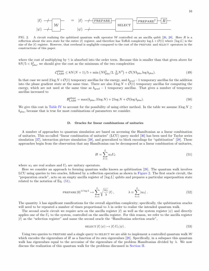
FIG. 2. A circuit realizing the qubitized quantum walk operator W controlled on an ancilla qubit [26, 28]. Here R is areflection about the zero state for the entire |`〉 register, and therefore has Toffoli complexity logL+O(1) where dlogLe is thesize of the |`〉 register. However, that overhead is negligible compared to the cost of the prepare and select operators in theconstructions of this paper.

where the cost of multiplying by γ is absorbed into the order term. Because this is smaller than that given above for9N/5 < b2pha, we should give the cost as the minimum of the two complexities

CphaseLABS ≤ 8N(N + 1)/5 + min

(Nb2pha/2,

910N

2)

+O(Nbpha log bpha). (49)

In that case we need 2 logN+O(1) temporary ancillas for the energy, and bgrad−1 temporary ancillas for the additioninto the phase gradient state at the same time. There are also 3 logN +O(1) temporary ancillas for computing theenergy, which are not used at the same time as bgrad − 1 temporary ancillas. That gives a number of temporaryancillas increased to

BphaseLABS = max(bpha, 3 logN) + 2 logN +O(log bpha). (50)

We give this cost in Table IV to account for the possibility of using either method. In the table we assume 3 logN ≥bpha, because that is true for most combinations of parameters we consider.

D. Oracles for linear combinations of unitaries

A number of approaches to quantum simulation are based on accessing the Hamiltonian as a linear combinationof unitaries. This so-called “linear combination of unitaries” (LCU) query model [36] has been used for Taylor seriessimulation [37], interaction picture simulation [38], and generalized to block encodings for “qubitization” [28]. Theseapproaches begin from the observation that any Hamiltonian can be decomposed as a linear combination of unitaries,

H =

L∑`=1

w`U` (51)

where w` are real scalars and U` are unitary operators.Here we consider an approach to forming quantum walks known as qubitization [28]. The quantum walk involves

LCU using queries to two oracles, followed by a reflection operation as shown in Figure 2. The first oracle circuit, the“preparation oracle”, acts on an empty ancilla register of dlogLe qubits and prepares a particular superposition staterelated to the notation of Eq. (51),

prepare |0〉⊗ logL 7→L∑`=1

√w`λ|`〉 , λ ≡

L∑`=1

|w`| . (52)

The quantity λ has significant ramifications for the overall algorithm complexity; specifically, the qubitization oracleswill need to be repeated a number of times proportional to λ in order to realize the intended quantum walk.

The second oracle circuit we require acts on the ancilla register |`〉 as well as the system register |ψ〉 and directlyapplies one of the U` to the system, controlled on the ancilla register. For this reason, we refer to the ancilla register|`〉 as the “selection register” and name the second oracle the “Hamiltonian selection oracle”,

select |`〉 |ψ〉 7→ |`〉U` |ψ〉 . (53)

Using two queries to prepare and a single query to select we are able to implement a controlled quantum walkWwhich encodes the eigenvalues of H as a function of its own eigenvalues [28]. Specifically, in a subspace this quantumwalk has eigenvalues equal to the arccosine of the eigenvalues of the problem Hamiltonian divided by λ. We nowdiscuss the realization of this quantum walk for the problems discussed in Section II.

17

1. LCU oracles for L-term Hamiltonian

Using the strategy for unary iteration introduced in [26] we can implement select for HL with Toffoli complexityof exactly L− 2 and dlogLe − 1 extra ancilla qubits (or L− 1 and dlogLe if the operation needs to be controlled byanother ancilla, as it is in [26]). The circuit given there has dlogLe ancilla. The other ancilla is just a control, it isn’tneeded for the iteration. If we don’t want to make it controlled, then the number of ancilla needed is dlogLe − 1.Also, the Toffoli cost is only L− 2 if we don’t need to make it controlled. The operator we are to implement is

select |`〉 |ψ〉 7→ |`〉∏i∈q`

Zi |ψ〉 . (54)

A simple way to understand the strategy would be to first map the binary representation of |`〉 to a one-hot unaryregister (a register that contains L qubits which are all off except for qubit ` which is on). Then, one could controlthe application of the Zi associated with i ∈ q` on this qubit with only Clifford gates. This strategy would have lowToffoli complexity but would require L ancilla. The basic insight of the unary iteration circuits in [26] is that onecan stream through bits of this unary register using just dlogLe − 1 extra ancilla. A circuit primitive is repeated Ltimes and at iteration j, a particular ancilla is equal to on if and only if ` = j. At that point in the circuit we canuse Clifford gates to control the application of Hamiltonian terms like ZiZjZk.

In [26] a strategy referred to therein as “coherent alias sampling” is introduced and explicit circuits are providedwhich allow one to realize prepare for an arbitrary model with a Toffoli cost of L + bLCU + logL + O (1). Weneed approximately logL ancillas for the state being prepared, logL for the alternate index values, and logL for thetemporary ancillas in the QROM. There are bLCU ancillas for the keep probabilities in the coherent alias sampling andbLCU for the equal superposition state. Another temporary ancilla is used for the result of the inequality test. selectuses L Toffolis and logL temporary ancilla, but these can be reused from the temporary ancilla used by prepare.Here, bLCU is a parameter that scales the precision of the cost function. In particular, this strategy will generate thestate in Eq. (52) but with approximate coefficients w` in place of the exact coefficients w` such that∣∣∣√w` −√w`∣∣∣ ≤ 2−bLCU . (55)

Per the realization depicted in Figure 2, the quantum walk of interest is realized using two queries to prepare andone query to select. Thus, the strategy we have outlined requires Toffoli and ancilla counts of

CLCUL = 3L+ 2 bLCU + 2 logL+O (1) , (56)

ALCUL = 2dlogLe+ 2 bLCU +O(1), (57)

BLCUL = dlogLe = logL+O(1). (58)

2. LCU oracles for QUBO and using dirty ancilla

In some cases, especially when there is some structure in the Hamiltonian terms and one is willing to reduce gatecomplexity at the cost of space complexity, another method of implementing prepare might be appropriate. Inparticular, we can combine the coherent alias sampling ideas of [26] with the on-the-fly “dirty QROAM” of [39](which is a concrete realization of an idea in [40] which builds on the QROM idea of [26] and is named “QROAM”since it incorporates attributes of both QROM and QRAM). Using Theorem 1 of [39] in conjunction with the coherentalias sampling of [26] with cost bLCU +O(logN), we see that it is possible to implement prepare with

2L

k+ 4 bLCU k +O (bLCU + k logL) (59)

Toffolis and (k− 1)bLCU dirty ancilla in addition to 2bLCU + log(L/k) +O(1) clean ancilla (not counting the selectionregister), where k ∈ [1, L] is a free parameter that must be a power of 2. This sort of QROAM can be uncomputedfaster than it can be computed [39]. Combining Theorem 3 in [39] with coherent alias sampling [26] leads us to theresult that the Toffoli cost of uncomputing prepare is less than the complexity quoted above by 4(bLCU − 1)k andcan reuse the same ancilla. The number of dirty ancilla is reduced to k − 1, which means that the value of k can betaken to be larger, reducing the Toffoli complexity. See Table V for detailed costs of various types of QROAM.

We will use this dirty QROAM strategy for the QUBO Hamiltonian. Our approach will involve indexing the termsand coefficients with two registers, each of size dlogNe so that |`〉 = |i〉 |j〉. This makes applying select particularlyeasy as we can use two applications of the unary iteration strategy that we discussed for implementing Eq. (54) to

18

type of ancilla type of computation Toffolis clean ancilla dirty ancilla

clean forward dL/ke+M(k − 1) dlog(L/k)e+M(k − 1) 0

dirty forward 2dL/ke+ 4M(k − 1) dlog(L/k)e M(k − 1)

clean reverse dL/ke+ k dlog(L/k)e+ k 0

dirty reverse 2dL/ke+ 4k dlog(L/k)e+ 1 k − 1

TABLE V. The QROAM complexities from [39], where L is the number of items, k is a power of 2, and M is the output size.This table omits the logL ancilla from the selection register and the M -qubit output.

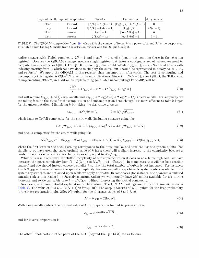
realize select with Toffoli complexity 2N − 4 and dlogNe − 1 ancilla (again, not counting those in the selectionregister). Because the QROAM strategy needs a single register that takes a contiguous set of values, we need tocompute a new register for QUBO. For QUBO where i ≤ j one would calculate j(j− 1)/2 + i. (Note that this is withindexing starting from 1, which we have done to simplify the sums, but 1 would be represented in binary as 00 . . . 00,and so forth.) We apply the QROAM to this register, then uncompute it afterwards. The cost of computing anduncomputing this register is O(log2N) due to the multiplications. Since L = N(N + 1)/2 for QUBO, the Toffoli costof implementing select, in addition to implementing (and later uncomputing) prepare, will be

2N2

k+ 4 bLCU k + 2N +O

(bLCU + log2N

)(60)

and will require kbLCU +O(1) dirty ancilla and 2bLCU + 2 log(N/k) + 2 logN +O(1) clean ancilla. For simplicity weare taking k to be the same for the computation and uncomputation here, though it is more efficient to take k largerfor the uncomputation. Minimizing k by taking the derivative gives us

4bLCU − 2N2/k2 = 0, k = N/√

2bLCU, (61)

which leads to Toffoli complexity for the entire walk (including select) going like

4N√

2bLCU + 2N +O(bLCU + log2N

)= 4N

√2bLCU +O(N) (62)

and ancilla complexity for the entire walk going like

N√bLCU/2 + 2 bLCU + 2 log bLCU + 2 logN +O(1) = N

√bLCU/2 +O(log(bLCUN)), (63)

where the first term in the ancilla scaling corresponds to the dirty ancilla, and thus can use the system qubits. Forsimplicity we have used the exact optimal value of k here; there will a slight increase to the complexity because kneeds to be a power of 2 so cannot be taken exactly equal to N/

√2bLCU.

While this result optimizes the Toffoli complexity of our implementation it does so at a fairly high cost; we haveincreased the space complexity from N +O(bLCU) to N

√bLCU/2+O(bLCU). In many cases this will not be a sensible

tradeoff and one should instead choose a smaller k so that the total number of qubits is not increased. For instance,k = N/bLCU will never increase the spatial complexity because we will always have N system qubits available in thesystem register that are not acted upon while we apply prepare. In some cases (for instance, the quantum simulatedannealing algorithm realized by Szegedy quantum walks) we will actually have 2N qubits available for use duringprepare and so we can safely take k = 2N/bLCU without increasing the spatial complexity.

Next we give a more detailed explanation of the costing. The QROAM costings are, for output size M , given inTable V. The value of L is L = N(N + 1)/2 for QUBO. The output consists of bLCU qubits for the keep probabilityin the state preparation, plus 2dlogNe qubits for the alternate values of i and j, so

M = bLCU + 2dlogNe. (64)

With clean ancilla qubits, the optimal value of k for preparation limited to powers of 2 is

kc1 = 2round(log√L/M), (65)

and for inverse preparation is

kc2 = 2round(log√L), (66)

The other Toffoli costs in other parts of the LCU (beyond the QROAM) are as follows.

19

• There is O(logN) cost to prepare the equal superposition states over i and j with i ≤ j.

• There is 2(bLCU+2 logN)+O(1) Toffoli cost for the inequality test and controlled swaps for the state preparationand inverse preparation.

• The cost of the arithmetic for producing the contiguous ancilla is O(log2N).

• The select has a Toffoli cost of 2N − 4, or 2N − 2 if it needs to be made controlled.

Altogether these costs give a Toffoli cost with clean ancilla of

N(N + 1)

2kc1+N(N + 1)

2kc2+M(kc1 − 1) + kc2 + 2bLCU + 2N +O

(log2N

), (67)

with the values of M , kc1, and kc2 in Eq. (64), Eq. (65), and Eq. (66). If we ignore the rounding in kc1 and kc2, thenthe Toffoli cost is √

2bLCUN +O(N + bLCU + b

−1/2LCU N logN

). (68)

The rounding in kc1 and kc2 can potentially increase the cost by a factor of 1/√

2 + 1/√

8, or about 6%.In costing the total number of ancillas for the state preparation, we also need to account for the following (in

addition to those in Table V).

• There are 2dlogNe qubits needed for the prepared state.

• There are bLCU qubits used for the register in equal superposition that we use to perform an inequality test within the state preparation.

• The M output qubits.

• There are dlogLe temporary ancilla qubits used for the contiguous register.

• There are bLCU − 1 temporary ancillas used in computing the inequality test for the state preparation.

There are also logN temporary registers needed for the select step, but many of the qubits are only temporarilyused by the QROAM, and these can be reused, so we do not get an additional ancilla cost for select. The ancillasadditional to those in Table V can therefore be given as 2M persistent ancillas and max(logL, bLCU)+O(1) temporaryancillas. The ancillas in Table V are temporary as well, and the bLCU qubits are not needed at the same time, givinga maximum of

log(L/kc1) +M(kc1 − 1) + logL+O(1), (69)

temporary ancillas. Ignoring the rounding in kc1 for simplicity gives the leading-order term as N√M/2 temporary

ancillas. Next we consider the cost with N dirty ancilla. The optimal value of k for the QROAM computation is

kd1 = 2blog(N/M+1)c. (70)

For the uncomputation cost it is optimal to take kd2 =√L/2 which gives a cost of 4

√2L, ignoring rounding of kd2

to a power of 2. With L = N(N + 1)/2, the optimal kd2 is√N(N + 1)/4 < N , so there are enough dirty ancilla

available. With rounding the value of kd2 for uncomputation would be

kd2 = 2round(log√N(N+1)/4). (71)

Together with the additional Toffoli costs for the state preparation, the Toffoli cost for LCU is

N(N + 1)

kd1+N(N + 1)

kd2+ 4M(kd1 − 1) + 4kd2 + 2bLCU + 2N +O(log2N). (72)

To simplify the expression, we will use N/M rather than N/M +1 in the expression for kd1, and not take into accountrounding k to a power of 2. Then we get a computation Toffoli cost of

CLCUQUBO = N(bLCU + 2 logN) +O(N). (73)

20

For the ancilla cost, the persistent ancilla cost is again 2M , and the temporary ancilla cost loses the term M(k− 1)because dirty ancilla are used for that, so it does not increase the ancilla cost. The temporary ancilla cost is

max(log(L/kd1) + logL, bLCU) +O(1). (74)

Using L = N(N+1)/2 and kd1 = N/M gives log(L/kd1) = log(N + 1)+logM−1. Then log(N + 1) = logN+O(1/N).Using M = bLCU + 2 logN +O(1) then gives

ALCUQUBO = 2 bLCU + 4 logN +O(1), (75)

BLCUQUBO = max(3 logN, bLCU) +O(log bLCU). (76)

In Table IV we just give 3 logN for the temporary ancilla cost, because it is true (or close to true) for the combinationsof parameters we consider.

3. LCU oracles for the SK model

For the SK model we can considerably improve over the naive implementation. Because the SK model coefficientsonly need to give a sign, we just need to apply a sign to the terms in the superposition. That corresponds to thephase fixup used for the QROAM uncomputation, and the cost is the same. Another advantage of this approach isthat we eliminate the 2(bLCU + 2 logN) +O(1) cost for the inequality test and controlled swaps that would otherwisebe needed for the coherent alias sampling. Therefore the Toffoli cost with clean ancilla is

N(N − 1)

2kc2+ kc2 + 2N +O

(log2N

). (77)

If we ignore the rounding in kc2 then we obtain the complexity

(2 +√

2)N +O(log2N

). (78)

Beyond the ancillas needed for the QROAM, we just need the 4 logN + O(1) qubits for the i, j, and contiguousregisters. Again select can use the same temporary ancillas as the QROAM and does not add to the ancilla cost.Therefore the ancilla cost is

log(L/kc2) + kc2 + 4 logN +O(1). (79)

Ignoring the rounding in kc2 for simplicity gives

N/√

2 +O (logN) . (80)

If we are using dirty ancilla, then the Toffoli cost becomes

N(N − 1)

kd2+ 4kd2 + 2N +O

(log2N

). (81)

Ignoring the rounding in kd2 we obtain the complexity

CLCUSK = 6N +O

(log2N

). (82)

The persistent ancilla cost is only 2 logN for the i and j registers, and there is temporary ancilla cost of 2 logN forthe contiguous register and log(L/kd2) ≈ logN from the QROAM. The total ancilla costs are therefore

ALCUSK = 2 logN +O(1), (83)

BLCUSK = 3 logN +O(1). (84)

4. LCU oracles for the LABS model

The LABS problem has L = O(N3) terms in it, which would lead a high complexity quantum walk if our generalstrategy were applied. Fortunately, there is much structure in this problem. We start by rewriting Eq. (6) as

HLABS =

N−1∑k=0

N−k∑j=1

N−k∑i=1

ZiZi+kZjZj+k. (85)

21

Instead of linearly indexing all O(N3) terms, we will use three registers, each of size logN , which store the values ofi, j and k. Thus, our select operation will act as

select |i〉 |j〉 |k〉 |ψ〉 7→ |i〉 |j〉 |k〉ZiZi+kZjZj+k |ψ〉 . (86)

To accomplish this, we simply need 4 applications of the unary iteration primitive described in [26]. Each of theseprimitives require N − 1 Toffoli gates. The only nuance is that we will need to compute the values i + k and j + kbefore implementing the primitive to perform Zi+k and Zj+k.

These additions can be performed in place (and then uncomputed) in the i and j registers and introduce a negligibleadditive 4 logN cost to the cost of unary iteration, where the cost of addition is dlogNe − 1 ≤ logN . Thus, the totalToffoli cost of our select implementation is 4N + 4 logN . We require approximately 3 logN persistent ancilla forthe i, j and k registers, another logN temporary ancilla for computing the i+ k and j + k (since they are computedin place), and logN temporary ancilla for the addition. The unary iteration uses dlogNe − 2 < logN ancillas, whichcan be reused from the temporary ancillas for the addition so do not add to the cost. Because all terms have the samecoefficient, prepare needs to initialize a superposition over a number of items that is not a power of 2. The Toffolicost is O(logN). The only unfortunate aspect is that for the LABS problem the corresponding normalization λ, isquite large and this will enter into the complexity of our quantum walks as the number of times the quantum walkmust be repeated to realize the intended unitary. In total then the cost to realize the quantum walk in Figure 2 is

CLCULABS = 4N +O(logN), (87)

ALCULABS = 3 logN +O(1), (88)

BLCULABS = 2 logN +O(1), (89)

λLABS ≈ N3/3. (90)

E. QROM-based function evaluation

Now that we have explained how to implement oracles for various cost functions of interest, we turn to the questionof how to calculate functions of the cost. This is important for several possible approaches to heuristic-based com-binatorial optimization. In simulated annealing, for instance, the probability of moving from one candidate solutionto another is proportional to an exponential of the energy difference between the two solutions, multiplied by aninverse temperature β. We would thus require the quantum computer to calculate an exponential of the output ofthe relevant energy difference oracle.

Because we are implementing heuristic approaches to combinatorial optimization, we do not expect that the func-tions of the cost need to be calculated to a high degree of accuracy so long as the functions we compute are stillmonotonic in the cost (to make sure that the energy landscape is not inverted in any way). We instead want tominimize the computational complexity of evaluating these functions given rather weak requirements on the accuracyof the output. Here we describe a general strategy for such cheap approximate function evaluation.

Our overall strategy is to approximate a function f of a b-bit input z by a piecewise linear approximation, f . Thisapproximation f is calculated based on a choice of sample points z0 < z1 < . . . < zg, where z0 ≤ z < zg. These samplepoints separate the interval [z0, zL) into g different sub-intervals of the form [z`, z`+1) with ` = 0, 1, . . . , g − 1. Theinput z belongs to exactly one of these sub-intervals, and so we find an ` such that z` ≤ z < z`+1. Having found `, we

use some data that can be looked up in order to calculate f(z) = αf(z`)+(1−α)f(z`+1) for α = (z`+1−z)/(z`+1−z`).That is, the function f is defined by interpolating between known values f(z`) and f(z`+1) of the target function f .

QROM [26] can be used to obtain the region that z is in (i.e. the correct value of ` above), and for that region theQROM outputs a slope and intercept for the linear approximation. The Toffoli cost of looking up one of g differentpossible values in the scheme of [26] is g−2, or g−1 if the output is controlled by a qubit. This Toffoli count relies ona technique from [32] in which certain naively expected Toffolis can be replaced with Clifford gates plus measurement.Also note that the Toffoli count of QROM-based lookup is independent of the number of bits of data output, meaningthat we are free to choose any number of bits to represent the slope and intercept without introducing a Toffolicost from the QROM. We choose the number of bits in order to obtain bsm bits for f . That is, f may be a roughapproximation of f , but we give f to more bits than needed by that approximation so f has smooth behaviour.

We will not use QROM precisely as specified in [26] but rather a variant of it. To explain the distinction, we beginwith some terminology. QROM is a method for executing a quantum circuit that operates on two registers, an inputregister and an output register. The input register has an initial value of ` encoded into it and the output registerstarts in the all-zero state. Each value of ` corresponds to some piece of data d` that has been specified classicallybefore the quantum circuit was constructed. The effect of the QROM is

QROM : |`〉input |0〉output 7→ |`〉input |d`〉output . (91)

22

•• •

• •• •• • •

• • • • • •• • • • • • • •• • • • • • • •• • • •

? ? ? ? ? ? ? ?

? ? ? ? ? ? ? ?

? ? ? ? ? ? ? ?

? ? ? ? ? ? ? ?

? ? ? ? ? ? ? ?

? ? ? ? ? ? ? ?

? ? ? ? ? ? ? ?

? ? ? ? ? ? ? ?d0 d1 d2 d3 d4,5 d6,7 d8−11 d12−15

••

••• • •

• • • •• • • •• • • •• •

? ? ? ? ?

? ? ? ? ?

? ? ? ? ?

? ? ? ? ?

? ? ? ? ?

? ? ? ? ?

? ? ? ? ?

? ? ? ? ?d0 d1 d2,3 d4−7 d8−15

(a) (b)

FIG. 3. (a) This figure shows how to perform QROM with variable spacing for the example where there are 4 bits, and weaim to group the input numbers as 0, 1, 2, 3, 4, 5, 6, 7, 8, 9, 10, 11, 12, 13, 14, 15. That is, we output the same datafor inputs of 4 and 5, and so forth. The first four lines are the four input bits and the fifth is a control register. There are 6Toffolis needed in this example for 8 data points, with one more Toffoli for a control. (b) This figure shows how to performQROM with variable spacing for the example where there are 4 bits, and we group the input numbers by powers of 2 as 0, 1,2− 3, 4− 7, and 8− 15. There are 3 Toffolis needed in this example for 5 data points, with one more Toffoli for a control.

Our variant of QROM is designed for the case in which there are data collisions. That is to say, we consider thecase where d` = d`′ for several different pairs ` and `′. In Figure 3(a) we explain how this QROM variant works forL = 16 in the case where d4 = d5, d6 = d7, d8 = d9 = d10 = d11, and d12 = d13 = d14 = d15. In this variant, weimagine that we have distinct parts of the iteration: iterate by ` 7→ `+ 1, iterate by ` 7→ `+ 2, iterate by ` 7→ `+ 4,and so on for each power of two. This variant of QROM is appropriate for our purposes because we want to improvecomputational efficiency by spacing z` unevenly. This is equivalent to treating many pieced of data d` as being equal,as the data is simply the information needed to calculate a linear function. The total number of Toffoli gates is stillg − 2 for g distinct regions, provided these regions correspond to ignoring bits of the input. For example, we can usea region such as 4, 5, but not 3, 4, because 4 ≡ 100 and 5 ≡ 101, so grouping 4 and 5 corresponds to ignoring theleast significant bit, but the least significant bit changes between 3 and 4.

A further subtlety is that all regions need to be a size corresponding to a power of 2 for this cost. In some caseswe may wish to have a final region that is larger than half, so it is not a size that is a power of 2. That will occurbecause we can have a large energy difference, but the exponential will give a transition probability that will just beapproximated as zero for a wide range of energies. Then the cost can be larger. For example, if we are distinguishing 0from 1− 15, then it will take 3 Toffolis. The cost can be seen from the diagram where the size of the regions increasesin powers of 2, shown in Figure 3(b). There one can choose the numbers used for d4−7 and d8−15 to be equal, whichgives a region for 4 − 15. This choice corresponds to a situation where the gap between neighboring interpolationpoints z` grows exponentially.

For many of the piecewise approximations, we can obtain accurate approximations using just powers of 2, as inFigure 3(b). Two main types of function that we aim to approximate are the exponential and the arcsine of theexponential. For the exponential the piecewise approximation can use points at argument values of 0, 1/2, 1 and soon and achieve a piecewise linear approximation within about 0.03. The arcsine of the exponential is more difficult toapproximate because the slope diverges at an argument of 0, but using piecewise linear approximation points startingat 1/211 and going up by powers of 2 gives similar precision as for the exponential.

To estimate the number of interpolation points needed for higher precision, note that the error of interpolation offunction f(z) is approximately

(δz)2

8f ′′(z) , (92)

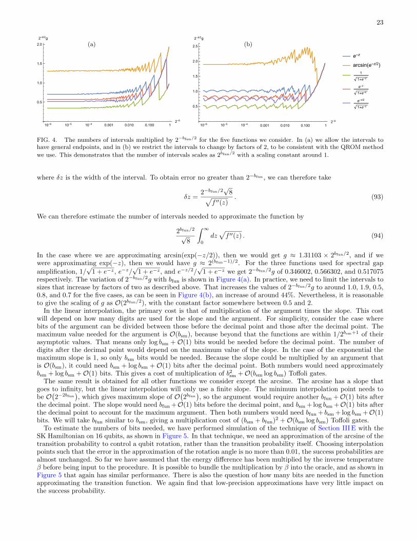
23

10-6 10-5 10-4 0.001 0.010 0.100 12-b

0.5

1.0

1.5

2.0

2-b/2g

10-6 10-5 10-4 0.001 0.010 0.100 12-b

0.5

1.0

1.5

2.0

2.5

2-b/2g

e-z

arcsin(e-z/2)

1

1+e-z

e-z

1+e-z

e-z/2

1+e-z

(a) (b)

FIG. 4. The numbers of intervals multiplied by 2−bfun/2 for the five functions we consider. In (a) we allow the intervals tohave general endpoints, and in (b) we restrict the intervals to change by factors of 2, to be consistent with the QROM method

we use. This demonstrates that the number of intervals scales as 2bfun/2 with a scaling constant around 1.

where δz is the width of the interval. To obtain error no greater than 2−bfun , we can therefore take

δz =2−bfun/2

√8√

f ′′(z). (93)

We can therefore estimate the number of intervals needed to approximate the function by

2bfun/2√8

∫ ∞0

dz√f ′′(z) . (94)

In the case where we are approximating arcsin(exp(−z/2)), then we would get g ≈ 1.31103 × 2bfun/2, and if wewere approximating exp(−z), then we would have g ≈ 2(bfun−1)/2. For the three functions used for spectral gap

amplification, 1/√

1 + e−z, e−z/√

1 + e−z, and e−z/2/√

1 + e−z we get 2−bfun/2g of 0.346002, 0.566302, and 0.517075respectively. The variation of 2−bfun/2g with bfun is shown in Figure 4(a). In practice, we need to limit the intervals tosizes that increase by factors of two as described above. That increases the values of 2−bfun/2g to around 1.0, 1.9, 0.5,0.8, and 0.7 for the five cases, as can be seen in Figure 4(b), an increase of around 44%. Nevertheless, it is reasonableto give the scaling of g as O(2bfun/2), with the constant factor somewhere between 0.5 and 2.

In the linear interpolation, the primary cost is that of multiplication of the argument times the slope. This costwill depend on how many digits are used for the slope and the argument. For simplicity, consider the case wherebits of the argument can be divided between those before the decimal point and those after the decimal point. Themaximum value needed for the argument is O(bsm), because beyond that the functions are within 1/2bsm+1 of theirasymptotic values. That means only log bsm + O(1) bits would be needed before the decimal point. The number ofdigits after the decimal point would depend on the maximum value of the slope. In the case of the exponential themaximum slope is 1, so only bsm bits would be needed. Because the slope could be multiplied by an argument thatis O(bsm), it could need bsm + log bsm +O(1) bits after the decimal point. Both numbers would need approximatelybsm + log bsm +O(1) bits. This gives a cost of multiplication of b2sm +O(bsm log bsm) Toffoli gates.

The same result is obtained for all other functions we consider except the arcsine. The arcsine has a slope thatgoes to infinity, but the linear interpolation will only use a finite slope. The minimum interpolation point needs tobe O

(2−2bfun

), which gives maximum slope of O

(2bfun

), so the argument would require another bfun +O(1) bits after

the decimal point. The slope would need bfun +O(1) bits before the decimal point, and bsm + log bsm +O(1) bits afterthe decimal point to account for the maximum argument. Then both numbers would need bfun + bsm + log bsm +O(1)bits. We will take bfun similar to bsm, giving a multiplication cost of (bsm + bfun)2 +O(bsm log bsm) Toffoli gates.

To estimate the numbers of bits needed, we have performed simulation of the technique of Section III E with theSK Hamiltonian on 16 qubits, as shown in Figure 5. In that technique, we need an approximation of the arcsine of thetransition probability to control a qubit rotation, rather than the transition probability itself. Choosing interpolationpoints such that the error in the approximation of the rotation angle is no more than 0.01, the success probabilities arealmost unchanged. So far we have assumed that the energy difference has been multiplied by the inverse temperatureβ before being input to the procedure. It is possible to bundle the multiplication by β into the oracle, and as shown inFigure 5 that again has similar performance. There is also the question of how many bits are needed in the functionapproximating the transition function. We again find that low-precision approximations have very little impact onthe success probability.

24

70

80

90

Cost

est

imat

e

20 / 0.48 30 / 0.72 40 / 0.96 50 / 1.2Number of annealing steps / Value of

0.4

0.6

0.8

Failu

re p

roba

bilit

y

Exact

Interpolated

Include

Rounded output

FIG. 5. The effect of various methods of function approximation on optimization performance. We numerically simulate thequantum simulated annealing technique of Section III E using various methods of approximating the transition probability. Weconsider the performance when the rotation angle is calculated to machine precision (“exact”), with piecewise linear approxima-tion chosen to ensure the worst-case error does not exceed 0.01 (“interpolated”), incorporating the inverse temperature β intothe definition of the function so that we are interpolating f(z) = arcsin(exp(−βz/2)) rather than f(z) = arcsin(exp(−z/2)) toavoid a multiplication (“include β”), and when we round off the output of the function to 7 bits (“rounded output”). Each ofthese approximations builds upon the previous approximation, so we perform linear interpolation in all but the exact method.We simulate the performance averaging over 4096 random SK instances on 16 qubits, with β linearly increasing over 50 stepsfrom 0 to 1.2. We report the average failure probability (bottom) as well as an estimate of the computational cost (top) in whichwe calculate the number of annealing steps divided by the probability of success. We observe that the differences in perfor-mance are not meaningfully affected by the method of function approximation, suggesting that we can pick the computationallycheapest option for our cost analysis.

The overall complexity of the interpolation excluding the QROM is therefore bsm +O(bsm log bsm) or (bsm + bfun)2 +O(bsm log bsm) when the arcsine is needed. To estimate the QROM complexity, we need to account for the final regionnot being a size which is a power of 2. In the worst case the additional cost can be no larger than bdif , which isthe total size of the input register. We can therefore bound the QROM complexity as bdif +O(2bfun/2), giving totalinterpolation complexity of

Cfun = b2sm + bdif +O(bsm log bsm + 2bfun/2), (95)

or, for the case where the arcsine is needed,

Cfun = (bsm + bfun)2 + bdif +O(bsm log bsm + 2bfun/2). (96)

For the number of ancilla qubits needed, except for the arcsine case there are 2bsm +O(log bsm) needed for the slopeand intercept, and 2bsm +O(log bsm) used as temporary ancillas for the arithmetic. We need bdif−1 temporary ancillasfor the QROM, which is more than the number used for the arithmetic. The output for the transition probability canbe added into the slope, so does not increase the ancilla cost. Therefore the ancilla costs are

Afun = 2bsm +O(log bsm), (97)

Bfun = bdif − 1. (98)

These considerations give the costs for function evaluation in Table IV. For the arcsine case we need 2bsm + bfun +O(log bsm) ancillas for the slope and intercept, because we need another bfun ancillas for the slope. Again the temporaryancilla cost is primarily for the QROM, so the ancilla costs are

Afun = 2bsm + bfun +O(log bsm), (99)

Bfun = bdif − 1. (100)

25

III. OPTIMIZATION METHODS

In this section we review proposals for heuristic quantum optimization algorithms and explain how those algorithmscan be implemented in terms of the oracles we describe in Section II. By this we include methods based on Hamiltonianwalks, those based on time evolution, and methods related to simulated annealing. In most cases we will suggestimprovements to these methods, but an important motivation for this section is to give a complete analysis of thecomplexity of these algorithms which includes constant factors so that we can estimate the resources required torealize them in the surface code in Section IV. We describe the complexities of these methods in terms of the oraclesfrom the previous section in Table VI, then give the complexity in terms of Toffoli or T gates in Table VII.

As this section incorporates a wide variety of sophisticated techniques, we begin with a brief summary of theapproaches we are considering.

• Amplitude amplification (Section III A). We start by considering amplitude amplification, which can be used todirectly amplify the amplitude of the solution. Unlike the other methods, it takes no advantage of the structureof the solution, so is a useful reference point to compare to the other optimization approaches. Amplitudeamplification can also be used in combination with the other optimization approaches, by performing amplitudeamplification on the output of the optimization.

• The Quantum Approximate Optimization Algorithm (Section III B). The steps of this approach (QAOA) areequivalent to Trotter steps, so the costing for QAOA and Trotter steps is given in the same lines in Table VI andTable VII. Trotter steps can be used for adiabatic approaches, which are considered in the next subsection. Buthere we also focusing on strategies for efficiently estimating the QAOA objective value that are more appropriatefor a fault-tolerant cost model than standard approaches.

• Adiabatic quantum optimization (Section III C). We review the quantum adiabatic algorithm [2] and the moststraightforward way of implementing that approach using a Trotter method that queries the phase oraclespresented in Section II. We will then suggest a strategy for implementing the adiabatic algorithm using theLCU oracles presented in Section II. The LCU oracles have a different costing to Trotter/QAOA, so are given inseparate lines in Table VI and Table VII. Next, we will review a method for digitizing the adiabatic algorithmwhile suppressing certain types of errors that is based on inducing quantum Zeno-effect-like projection to theground state by randomizing phases [21]. We will suggest how this approach can be improved by using carefullychosen probability distributions to eliminate the errors that would manifest from incorrect measurements in theZeno approach. The time-evolution oracles used by these methods are also suitable for the quantum enhancedpopulation transfer algorithm and the shortest path algorithm. Since we do not introduce new techniques forthose algorithms, but rather review how our oracles can be queried within those frameworks, we discuss thatcontent in Appendix E.

• Szegedy walk based quantum simulated annealing (Section III D). Simulated annealing is a classical algorithmthat mimics a physical cooling process via Markov chain Monte Carlo techniques. The quantum algorithm ofSomma et al. [13] is to replace the Markov chain with a corresponding Szegedy walk. If the spectral gap of the

Markov transition operator is ∆, the number of Szegedy walk steps grows as O(1/√

∆) in contrast with the bestknown bound on the worst case scaling of the number of Markov transitions needed in the classical approach,which goes like O(1/∆). Thus, the result appears to be a quadratic speedup over simulated annealing. We notethat the O(1/∆) scaling of classical simulated annealing is known to be a very loose bound for a broad classof problems. Typically, simulated annealing is used heuristically by lowering the temperature much faster thanwould be suggested by this bound. Our results constitute the first complete cost analysis for this algorithm thatinvolves constant factors in the complexity.

• LHPST qubitized walk based quantum simulated annealing (Section III E). Lemieux, Heim, Poulin, Svore, andTroyer (LHPST) [23] give a Metropolis-Hastings-like qubitized walk approach which is significantly more efficientthan the direct Szegedy approach. We will refer to this method by their initials, but we provide an improvedtechnique that is efficient for more complicated problem Hamiltonians with high connectivity. LHPST considera method that is efficient for simpler problem Hamiltonians with low connectivity, but would have exponentialcost for the problem Hamiltonians considered here.

• Spectral gap amplification based quantum simulated annealing (Section III F). In [14], the authors construct aninverse-temperature-dependent Hamiltonian whose ground state in the zero-temperature limit is a superpositionof solution configurations. By performing spectral gap amplification on their Hamiltonian, they obtain a gapthat is similar to that for the quantum walk approach, indicating a similar speedup. Our main purpose is tooutline these techniques and summarize the work needed to execute such algorithms in general and for specific

26

algorithm primitive Toffoli complexity ancilla complexity

amplitude amplification step 2 Cdirect +N +O(bdir) (108) Adirect + Bdirect +O(1)

QAOA/Trotter step Cphase + 4N + b2pha/2 +O(bpha log bpha) (137) Aphase + max(Bphase, 3 logN) + bpha +O(log bpha)

Hamiltonian walk step CLCU +O(1) ALCU + BLCU +O(1)

Szegedy walk annealing step min(2(N + 1)Cdirect, 2NCdiff) + 2NCfun + 2N logN + 8Nbsm + 18b2sm +O(N) (190) NAdiff +NAfun + 5bsm +O(N) (191)

LHPST walk annealing step 2Cdiff + 2Cfun +N + 2bdif + 9 logN +O(1) (214) Adiff +Afun + Bdiff + logN + bsm +O(1) (215)

gap amplified walk step 2Cdiff + 2Cfun + 2bsm +N + 14 logN +O(brot) (233) Adiff +Afun + Bdiff + 2 logN + bsm +O(1) (234)

TABLE VI. The Toffoli complexities and ancilla complexities needed to implement the basic primitives of various heuristicalgorithms, reported in terms of the oracle costs from Table III. For both the LHPST walk step and the gap amplified walk stepthe cost is reduced by 8 logN when N is a power of 2. By combining these scalings with the oracle costs given in Table IV, wearrive at the resource estimates in Table VII. For order ρ Suzuki (meaning that the error is O

(δtρ+1

)) we multiply the QAOA

cost by 2× 5ρ/2−1. For the QAOA/Trotter step, the bpha ancillas are for a phase gradient state, and may be saved if those arealready accounted for in Aphase. The quantity ε is an allowable error in synthesizing a rotation in the state preparation.

problems of interest as outlined in the Introduction. We will also suggest a variant of this algorithm where onecan use qubitized quantum walks rather than time evolution for the adiabatic evolution. In both cases, ourresults provide the first constant factor bounds on the complexity of implementing these algorithms.

We summarize the outcomes of this section in Table VI. The entries of Table VI show how the Toffoli complexityand ancilla cost of each of the above named algorithm primitives depend on the relevant costs of oracles presented inTable IV. We can then use Table VI together with Table IV to calculate the overall Toffoli complexity and ancilla costof each algorithm primitive for each type of cost function. The results of this analysis are summarized in Table VII.In giving the complexities in this table, we assume 2bfun/2 < bsm log bsm < brot to simplify the order terms, which isreasonable for the examples we consider in Section IV.

A. Amplitude amplification

1. Combining amplitude amplification with quantum optimization heuristics

All of the optimization heuristics discussed in this paper can be seen as methods of preparing a quantum state withoverlap on a low energy subspace of interest. We will refer to the subspace of interest as S. Sometimes this subspaceof interest is actually the lowest energy state (or states) and other times it is any state with energy less than a certainthreshold. Furthermore, all algorithms discussed in this paper are heuristics that can be systematically refined. Let usrefer to an algorithm for quantum optimization that is run for duration t as U(t). Let us assume that these algorithms

always begin in the state |+〉⊗N and denote the output state of the algorithm by |ψ(t)〉 = U(t) |+〉⊗N . Thus, afterrunning our algorithm U(t) and sampling in the computational basis, the probability of measuring a state in thesubspace of interest S is

p0(t) =∑x∈S|〈x|ψ(t)〉|2 . (101)

When we say that these heuristics can be systematically refined what we mean is that we can (on average) increasep0(t) by increasing t. This refinement will come at a cost C(t) > 0 which we define as the complexity of implementing

U(t). This complexity is greater than zero because preparing the initial state |+〉⊗N requires nonzero time even ifwe do nothing further. We can also boost the probability of seeing a state in S by repeating U(t) more times andsampling. On average we will need to run our algorithm U(t) a number of times equal to 1/p0(t) in order to see astate in S. Thus, on average the cost to sample a state S is given by

C (t)

p0(t). (102)

There is a compromise to be reached between the duration t of the optimization heuristic U(t) and the successprobability p0(t); heuristics run for more time can reach a higher success probability and therefore be repeated fewertimes, but increasing t beyond a certain point has a negligible impact on its success probability p0(t). While past work[23] has discussed this dichotomy in terms of a minimum time to solution metric which is parameterized in terms of atarget success probability, here we focus on the mean cost to succeed because this seems more reasonable to considerin a context where p0(t) is unknown. Still, given knowledge of p0(t) one could optimize this mean time by choosing t

27

cost function algorithm primitive Toffoli (* or T) count total ancilla qubits

L-term amplitude amplification step 2L bdir +N +O(bdir) 2 bdir +O(1)

Spin QAOA/Trotter step* 1.15L(bpha + logL) +O(N + logL+ b2pha) 3 logN + bpha +O(log bpha)

Model Hamiltonian walk step 3L+ 2bLCU +O(logL) 3 logL+ 2 bLCU +O(1)

HL Szegedy walk annealing step 2(N + 1)Lbdir + 2N(b2sm + bdif + logN) +O(Nbsm log bsm) Nbdif + 2Nbsm +O(N log bsm)

LHPST walk annealing step 4Lbdif + 2(bsm + bfun)2 + 2bdif +N + 9 logN +O(bsm log bsm) 3bsm + 2bdif + bfun + logN +O(log bsm)

gap amplified walk step 4Lbdif + 2b2sm + 2bdif +N + 14 logN +O(brot) 3bsm + 2bdif + 2 logN +O(log bsm)

Quadratic amplitude amplification N2bdir +O(Nbdir) 2 bdir +O(1)

Unconstrained QAOA/Trotter step* 0.575N2(bpha + 2 logN) +O(N2) 3 logN + bpha +O(log bpha)

Binary Hamiltonian walk step N(bLCU + 2 logN) +O(N) 7 logN + 2 bLCU +O(log bLCU)

Optimization Szegedy walk annealing step 2N2bdif + 2N(b2sm + bdif + logN) +O(Nbsm log bsm) Nbdif + 2Nbsm +O(N log bsm)

HQUBO LHPST walk annealing step 2Nbdif + 2(bsm + bfun)2 + 2bdif +N + 9 logN +O(bsm log bsm) 3bsm + 2bdif + bfun + logN +O(log bsm)

gap amplified walk step 2Nbdif + 2b2sm + 2bdif +N + 14 logN +O(brot) 3bsm + 2bdif + 2 logN +O(log bsm)

Sherrington– amplitude amplification step 2N2 +N +O(logN) 6 logN +O(1)

Kirkpatrick QAOA/Trotter step 2N2 + 4N + b2pha +O(bpha log bpha) 6 logN + bpha +O(log bpha)

Model Hamiltonian walk step 6N +O(log2 N) 5 logN +O(1)

HSK Szegedy walk annealing step 4N2 + 2N(b2sm + 2 logN) + 8Nbsm + 18b2sm +O(Nbsm log bsm) N logN + 2Nbsm +O(N log bsm)

LHPST walk annealing step 5N + 2(bsm + bfun)2 + 11 logN +O(bsm log bsm) 4 logN + 3bsm + bfun +O(log bsm)

gap amplified walk step 5N + 2b2sm + 16 logN +O(brot) 5 logN + 3bsm +O(log bsm)

Low amplitude amplification step 5N(N + 1)/2 +N +O(logN) 5 logN +O(1)

Autocorrelation QAOA/Trotter step 8N2/5 + min(Nb2pha/2, 9N

2/10)

+O(Nbpha log bpha) 5 logN + bpha +O(log bpha)

Binary Hamiltonian walk step 4N +O(logN) 5 logN +O(1)

Sequences Szegedy walk annealing step 5N(N + 1)2/2 + 2N(b2sm + 3 logN) +O(Nbsm log bsm) 2N logN + 2Nbsm +O(N log bsm)

HLABS LHPST walk annealing step 5N2 + 2(bsm + bfun)2 + 6N + 13 logN +O(bsm log bsm) 6 logN + 3bsm + bfun +O(log bsm)

gap amplified walk step 5N2 + 2b2sm + 6N + 18 logN +O(brot) 7 logN + 3bsm +O(log bsm)

TABLE VII. Resource estimates for the various heuristic optimization primitives explored throughout this paper, applied toour four problems of interest. For both the LHPST walk step and the gap amplified walk step the Toffoli count is reduced by8 logN when N is a power of 2. In all cases, these algorithms are refined by applying the primitive more times. The parametersused are as follows: N is the number of bits on which our cost function is defined; L is the numbers of terms in an L-term spinHamiltonian; bpha is the number of bits we use to approximate phases in the implementation of our phase oracle; bdir is thenumber of bits we use to approximate the value of energies; bLCU is the number of bits used to approximate the square root ofHamiltonian coefficients in LCU methods, and brot is the number of bits of precision used in rotations. The Trotter step andHamiltonian walk steps can be used to realize the adiabatic algorithm, the Zeno phase randomization variant of the adiabaticalgorithm, heuristic variants of the short path algorithm or quantum enhanced population transfer, and many other heuristicsbased on Hamiltonian time evolution. These scalings result from combining the query complexities in Table VI with the oraclecosts in Table IV. When the algorithm type is decorated with (*) we report T complexity rather than Toffoli complexity. Wehave only given the main terms in the order expressions to simplify them.

to minimize Eq. (102). But rather than simply repeating the state preparation 1/p0(t) times, one could instead boostthe success probability with amplitude amplification.

Amplitude amplification is an idea which generalized Grover search and can be used to boost the probability of amarked state or subspace. For instance, we might define these marked states to be any state in S. In this context,amplitude amplification would allow us to perform a series of m reflections (involving two preparations of the state|ψ(t)〉) which boosts the probability of measuring the marked subspace to

pm(t) = sin2(

(2m+ 1) arcsin(√

p0(t)))

. (103)

For instance, if we hoped to boost the probability to 1 then by using repeated sampling we would need roughlyO(1/p0(t)) repetitions. However, by using amplitude amplification we would need only

m ≈ π

4 arcsin(√

p0(t)) − 1 = O

(1√p0(t)

)(104)

iterations if p0(t) is small (this is akin the usual quadratic Grover speedup).For each round of amplitude amplification one needs to reflect about a qubit marking the subspace of interest S.

In our context the idea would be to amplify either a target energy (if a target energy, e.g. the ground state energy, isknown) or to amplify all states with energy less than a certain threshold. To do this, one will need to compute theenergy value into a register and perform either an equality or inequality test to determine whether we have reached

28

a marked state. The energy can be computed simply by using the direct energy oracles introduced in Section II A.However, both that step and the cost of the equality or inequality evaluation will typically have a negligible additivecost to the cost C(t) of actually running the quantum algorithm U(t). Moreover, the ancilla used for storing the valueof the energy can be borrowed from ancilla used in other parts of the algorithm.

For amplitude amplification to be most effective one should have an estimate of the overlap p0(t) in order to avoid“overshooting” the peak of the function in Eq. (103). Unfortunately, a reliable estimate of p0(t) will not be knownin advance in general. In some rare cases one might instead have a somewhat tight estimate of a lower bound top0(t) and in those cases some advantages can be realized by using a variant of amplitude amplification known as fixedpoint amplitude amplification [41]. However one can confirm that fixed point amplitude amplification will have noadvantages in our context compared to the exponential search heuristic proposed in [20] when the best lower boundthat is available is p0(t) > 0. The idea behind the approach in [20] is to run amplitude amplification for m = 2j

iterations for j = 0, 1, 2, 3, ... and so on until we sample a marked state. The cost of each iteration of amplitudeamplification is 2 C(t) and so if we need to repeat this procedure until m = 2k it will have a total cost that goes like

2 C (t)

k∑j=0

2j = 2 C (t)(2k − 1

). (105)

Therefore, since the probability of failure in a single run with m = 2j iterations is 1− p2j (t), we see that the overallmean cost of the procedure is

2 C (t)

∞∑k=1

(2k − 1

) k−1∏j=1

(1− p2j−1(t)) = O(C (t)√p0(t)

). (106)

Though the left side of this expression cannot be simplified analytically, it converges quickly and can be easilynumerically computed for any p0(t) > 0.

Comparing Eq. (102) to Eq. (106) we can see that there is a clear asymptotic advantage to using amplitudeamplification over classical sampling and expect this advantage will be realizable in practice in many contexts of interestfor us. Like with Eq. (102), if one has knowledge of p0(t) then one can minimize Eq. (106) with respect to t to makethe optimal tradeoff between running the algorithm U(t) for longer and using more rounds of amplitude amplification.In some cases it might actually be the case that the optimal choice is t = 0, which would correspond to usingamplitude amplification directly as a heuristic for optimization. The only downside to using amplitude amplificationin conjunction with other heuristic quantum algorithms for optimization is that we have traded incoherent repetitionsof the primitive of U(t) for coherent repetitions of the primitive of U(t). In some cases this will mean that we need totarget a higher error rate to make the calculation fault-tolerant by using an error-correcting code.

2. Directly using amplitude amplification

In the prior section we described how amplitude amplification can be combined with any of the other optimizationheuristics in this paper in order to boost overlap on a target low energy subspace of interest. However, one canalso use amplitude amplification by itself as a heuristic for optimization. This heuristic provides an interesting pointof comparison to other algorithms because it offers a quadratic advantage over classical brute force search withoutleveraging any structure that might be available in a particular optimization problem. Thus, it is asymptoticallythe optimal strategy for solving totally unstructured problems like those described by the typical Grover oracle (allcomputational basis states have energy zero except for a solution with energy −1) or the random energy model (allcomputational basis states have a unique, Gaussian distributed energy).

To use amplitude amplification on its own all one needs to do is to regard the algorithm U(t) as the preparation

of the symmetric superposition state |+〉⊗N , which requires only Clifford gates. In the analysis of Section III A 1we assumed that the cost of directly computing the energy and then performing the comparison operation would benegligible compared to the cost of applying U(t) but that is not the case when we aim to directly apply amplitudeamplification. Here, the main cost of a step will be the cost to compute (and then later uncompute) the energy.Following Eq. (106), in this context we would find that the mean cost of applying amplitude amplification directlywill then scale like

(2 Cdirect +N +O (bdir)

) ∞∑k=1

(2k−1

) k−1∏j=1

(1−sin2

((2j+1

)arcsin

(√1

2N

)))= O

((Cdirect +N +O (bdir)

)√2N)

(107)

29

where we have used p0(t) = 1/2N . The cost 2 Cdirect + N + O (bdir) comes from cost Cdirect to directly compute theenergy, cost O (bdir) to apply the inequality operator to determine whether the energy is below the target threshold,cost Cdirect to uncompute the energy, and cost N − 2 to reflect about the equal superposition state. Note that thisprocedure is exactly the heuristic approach introduced in [20]. When the subspace S contains only a single state thisalgorithm reduces exactly to standard Grover search [3]. For later comparisons in this paper we will refer to the costof a single step of amplitude amplification as having

2 Cdirect +N +O (bdir) (108)

Toffoli complexity and requiring Adirect + Bdirect +O(1) ancilla.

B. The Quantum Approximate Optimization Algorithm

The quantum approximate optimization algorithm (QAOA) is another popular approach to quantum optimization,introduced in [12]. The QAOA initially attracted significant interest after it was shown to produce a better approxi-mation ratio for a specific combinatorial optimization problem of bounded occurrence, Max E3LIN2, than any knownefficient classical method [12]. While a more efficient classical algorithm was presented shortly afterwards [42], interestin QAOA has only increased since then. While bounds on the performance of QAOA are sometimes available, in mostcontexts it is studied as a heuristic in the sense that the intention is to use the algorithm without knowing how well itwill perform in practice. Part of the appeal of QAOA has been that it is an easy-to-implement algorithm that can betested on noisy intermediate scale quantum (NISQ) devices even before fault-tolerance is available [43]. Nonetheless,QAOA would still be an interesting algorithm to perform within error-correction.

The QAOA is more straightforward than other algorithms discussed in this work. The QAOA consists of twocomponents that are repeatedly applied. The first component is parameterized evolution under the diagonal problemHamiltonian C,

UC (γ) = e−iγC = Ophase (γ) , (109)

where in the last equality we emphasize that UC(γ) is equivalent to the phase oracle Ophase(γ) that we introduce andprovide explicit circuit constructions for in Section II C.

The second component is parameterized evolution under a local transverse field driver Hamiltonian B,

UB (β) = e−iβB B =

N∑j=1

Xj . (110)

The QAOA is a variational algorithm that uses repeated application of these unitaries to prepare a parameterizedstate that is then optimized. The depth of the variational algorithm is usually denoted as “p” in the QAOA literature.Specifically, for depth p we prepare a state parameterized by γ = (γ1, . . . , γp) and β = (β1, . . . , βp),

|γ,β〉 = UB (βp)UC (γp) . . . UB (β1)UC (γ1) |+〉⊗N (111)

where |+〉⊗N is the symmetric superposition of all 2N computational basis states.For a given p, we attempt to find parameters that minimize the expectation value of the cost

〈C〉 = 〈γ,β|C |γ,β〉 . (112)

The QAOA proposes to use the quantum computer to estimate this expectation value and then to use a classicalprocessor to perform a classical optimization, in a fashion similar to other variational algorithms [44, 45]. In generalfinding the globally optimal values of γ and β could prove to be very challenging. However, QAOA is a heuristicalgorithm and the idea is that even locally optimal parameter settings might provide good approximations.

The original implementation of QAOA suggested that one directly sample the cost function C to estimate 〈C〉.Using this method, if one wishes to converge an unbiased estimator 〈C〉 so that | 〈C〉 − 〈C〉 | ≤ ∆C then the state|γ,β〉 must be prepared and sampled a number of times equal to

σ2/∆2C where σ2 = 〈C2〉 − 〈C〉2 . (113)

While one will not know σ2 in advance, one can obtain a reasonable estimate of σ2 after only handful of measurementsand use that to determine how many more measurements are required.

30

The cost of QAOA is always dominated by the number of times that one must repeat the unitary UC(γ); the costto implement UB(β) is essentially free in comparison. Thus, if J is the number of outer-loop optimization iterationswhich each require a query of the energy accurate to within ∆C then in total we will require Toffoli complexity

p J Cphaseσ2

∆2C

. (114)

It is difficult to say what an appropriate choice of the quantities J and ∆C should be as this depends on the problem, thechoice of optimizer one is using, and how aggressively one is attempting to optimize. However, in many circumstancesone might not need to perform the outer-loop optimization at all and can thus take J = 1. This is the case whenoptimal (or “good enough”) parameters can be inferred before running the algorithm. Such a situation often ariseswhen running large instances of optimization problems that are characteristic of a well defined ensemble (for example,if one is running instances of the Sherrington-Kirkpatrick model). This is due to the observation that normalizedenergy landscapes (proportional to 〈C〉 as a function of γ and β) concentrate to instance and size independent averagevalues for large N [46, 47]. Thus, surprisingly, it is possible to find the optimal values of γ and β by optimizing muchsmaller (presumably classically tractable) instances of these problems. Another possibility is that one simply use γand β parameters that would be obtained from a Trotterization of the quantum adiabatic algorithm; in fact, there isevidence that these parameters become optimal as one increases p [48]. Thus, for problems where it is appropriateto forgo the outer-loop optimization step of QAOA, we can approximate the Toffoli complexity as pM Cphase whereM is the number of samples we desire. The number of logical qubits required for its implementation will be N (notcounting any extra ancilla used for the phase oracle).

Within the context of NISQ computations it makes sense to use this method of sampling to estimate the costfunction expectation value and then to perform the optimization on a classical computer. The reason is becauseboth strategies minimize the size of each quantum circuit that must be executed, although potentially at a cost ofneeding a larger number of repetitions compared to other strategies. However, within cost models appropriate forfault-tolerance the primary resource to consider is the total number of gates required by the computation and noparticular distinction is made whether those gates are involved in repeated applications of short quantum circuitsor a single application of a longer quantum circuit. Thus, on a fault-tolerant quantum computer it may make senseto consider more elaborate versions of QAOA in which the expectation value estimation and potentially even theoptimization is also performed on a quantum computer. For instance, perhaps the variational parameters γ and βcan be stored in a quantum register on which the QAOA unitary is controlled. Such a scheme is considered in [49]where it shown that such a method can enable quadratically faster resolution of the gradient than would be otherwiserequired, however with significant constant overhead. Similarly, by using the amplitude amplification based MonteCarlo techniques discussed in [50] (see Theorem 5 therein) one can reduce the number of state preparations needed

for an estimate of the cost function to O((σ/∆C) log3/2(σ/∆C) log log(σ/∆C)), an almost quadratic improvementover the naive sampling strategy. However, as that method requires a number of copies of the system register scalingas O(log(σ/∆C) log log(σ/∆C)), it might prove to be prohibitively expensive for realization on small fault-tolerantquantum computers. We now consider two alternative ways to measure the energy in QAOA which might prove morepractical for small fault-tolerant quantum computers.

1. Amplitude estimation based direct phase oracle evaluation

Apart from sampling, the next most natural algorithm for estimating the energy is using amplitude estimation tocompute the expectation value of each term in the cost function in sequence. Let us assume that the cost function

takes the form, C =∑L`=1 w`U`, where U` is a unitary operator (and will typically be a sum of diagonal Pauli

operators), as in Eq. (51). Further we will take λ =∑` |w`|. The algorithm that we employ is simple, for each ` from

1 to L we compute the quantity 〈ψ|U` |ψ〉 within error ∆C/(L|w`|). An unbiased estimate of the cost function is thengiven by

∑` w` 〈ψ|U` |ψ〉 and from the triangle inequality the error is at most ∆C .

An estimate of 〈ψ|U` |ψ〉 can be obtained by performing the Hadamard test (as shown in Figure 6). Specifically, theprobability of measuring the ancillary qubit to be zero is (1 + Re(〈ψ|U` |ψ〉))/2. If Amplitude Amplification is usedto mark the zero state for this circuit then the eigenphases of the resultant walk operator (within the two dimensionalspace spanned by the initial state and the marked state) is [20]

φ = ±2 arcsin(√

P0

)= ±2 arcsin

(√1 + Re (〈ψ|U` |ψ〉)

2

). (115)

We then have that

2 sin2(φ/2)− 1 = Re(〈ψ|U` |ψ〉). (116)

31

|0〉A H • H

|0〉 Uψ U`

FIG. 6. Hadamard test circuit for computing the expectation value of one of the terms in the cost-function. Here Uψ is aunitary operation that prepares the ansatz state: Uψ |0〉 = |ψ〉.

From calculus we then see that

∂φ(2 sin2(φ/2)) = 2 sin(φ/2) cos(φ/2) ≤ φ. (117)

Thus from Taylor’s remainder theorem we have that for any δ ≥ 0

|2 sin2(φ/2)− 2 sin2((φ+ δ)/2)| ≤ δ (118)

and if φ→ φ+ δ for some error δ we have that the uncertainty that propagates to the expectation value is at most

|Re(〈ψ|U` |ψ〉)− Re(〈ψ|U` |ψ〉)est| ≤ δ. (119)

Therefore if we wish to estimate the energy of a configuration within error ε it suffices to use phase estimation withan error of ε on the Grover operator. Finally, as discussed above we take ε = ∆C/(L|w`|) to ensure that the errorsums up to ∆C as required.

Using the QFT-based phase estimation algorithm in [26] we find that, if we neglect the cost of the Quantum FourierTransform and any additional costs due to additional precision required in the QROM then the number of queries tothe Grover oracle needed is (for ε ≤ π) 2m ≤ 2

⌊πε

⌋≤ 2π

ε . Here the factor of 2 comes from the fact that the need toround to a power of 2 leads to, in the worst case scenario, a factor of 2 in the number of iterations required.

Next the Grover oracle requires two reflection operators, one that reflects about the state yielded by the Hadamardtest circuit and another that reflects about the target space which is marked by the top qubit in Figure 6 being zero(i.e. R0 = 11−2 |0〉〈0|⊗11). The Grover walk operator is a product of these two operators W = −R1R0 and as a result,if we neglect the cost of the additional Hadamard and Toffoli gates needed to implement the conditional phase flip,the costs of this process are entirely due to the reflection about the initial state which requires two applications of thepreparation of the initial state. We further will follow the assumption in the previous section that the cost of statepreparation dwarfs the cost of applying prepare or select. Thus under these assumptions, and taking the uncertaintyin the objective function to be ∆C the Toffoli complexity for the entire simulation is approximately

L∑`=1

4pJπ|w`|LCphase

∆C=

4pJπλLCphase

∆C. (120)

Thus, under these assumptions, direct energy evaluation yields an advantage over sampling if

σ2 ≥ 4πλ∆CL. (121)

We expect this to occur when the error tolerance is small and the number of terms is relatively modest. On the otherhand if the variance is small, target uncertainty is large, or L is large then sampling will be preferable to the directphase oracle evaluation process.

2. Amplitude estimation based LCU evaluation

One inexpensive approach that can be used to estimate the expectation value comes from combining the Hadamardtest circuit and amplitude estimation [20]. Here we used a slightly generalized form of a generalized Hadamard testcircuit shown in Figure 7. The expectation value of the first qubit for the above circuit is 1/2 + Re(〈ψ|C |ψ〉)/2. In

32

|0〉A H • H

|0〉A prepareselect

prepare†|0〉A|0〉 Uψ

FIG. 7. Generalized form of a Hadamard test that we will use for our QAOA implementation using LCU oracles. Here Uψ isa unitary operation that prepares the ansatz state: Uψ |0〉 = |ψ〉.

order to see this, consider the following,

|0〉 |0〉 |ψ〉 7→ |0〉(∑

`

√w`λ|`〉)|ψ〉 7→ |0〉+ |1〉√

2

(∑`

√w`λ|`〉)|ψ〉

7→ |0〉√2

(∑`

√w`λ|`〉)|ψ〉+

|1〉√2

(∑`

√w`λ|`〉U` |ψ〉

)

7→ |0〉2

((prepare |0〉) |ψ〉+

∑`

√w`λ|`〉U` |ψ〉

)+|1〉2

((prepare |0〉) |ψ〉 −

∑`

√w`λ|`〉U` |ψ〉

)

7→ |0〉2

(|0〉 |ψ〉+ prepare†

∑`

√w`λ|`〉U` |ψ〉

)+|1〉2

(|0〉 |ψ〉 − |junk〉) . (122)

Therefore, the probability of measuring 0 in the top-most qubit in Figure 7 is

1

4

(2 + 〈0| 〈ψ|prepare†

∑`

√w`λ|`〉U` |ψ〉+

(〈0| 〈ψ|prepare†

∑`

√w`λ|`〉U` |ψ〉

)∗)=

1 + Re(〈ψ|C|ψ〉

λ

)2

. (123)

If amplitude estimation is used, the number of invocations of prepare and select needed to estimate this probabilitywithin ε error is O(λ/ε), which is a quadratic improvement over the sampling bound in Eq. (113).

Following the same reasoning used to derive Eq. (119) we find that the over all Toffoli count is then, under theassumptions that the Toffoli count is dominated by applications of the prepare, select and phase circuit operationsand further that the cost of adding an additional control to select is negligible, given by

4πpJλ(Cphase + CSel + 2CPrep)

∆C. (124)

Here CSel and CPrep are the Toffoli counts for select and prepare respectively.

Equation Eq. (124) shows that the favorable scalings of the sampling approach and the direct phase evaluationmethods can be combined together in a single method. However, this advantage comes potentially at the price of aworse prefactor owing to the additional complexity of the prepare and select circuits. In particular, we find thatthis approach will be preferable to sampling and direct phase estimation, respectively, when

σ2 ≥ 4πλ∆C

(Cphase + CSel + 2CPrep

Cphase

), (125)

L ≥ Cphase + CSel + 2CPrep

CPhase. (126)

In general, we suspect that in fault-tolerant settings this this approach will be preferable to direct phase oracleevaluation because the costs of the prepare and select circuits will often be comparable, or less than, that of Uψ aswe will see in the following section where we provide explicit constructions for the prepare and select oracles.

33

C. Adiabatic quantum optimization

1. Background on the adiabatic algorithm

The adiabatic algorithm [51] works by initializing a system as an easy-to-prepare ground state of a known Hamil-tonian, and then slowly (adiabatically) deforming that system Hamiltonian into the Hamiltonian whose ground statewe wish to prepare. For instance, we might use a Hamiltonian parameterized by s ∈ [0, 1],

H(s) = (1− s)H0 + sH1, (127)

where H0 is a Hamiltonian with an easy-to-prepare ground state and H1 is a Hamiltonian whose ground state wewish to prepare. We start the system in the ground state of H(0) = H0 and then slowly deform the Hamiltonian byincreasing s from 0 to 1 until H(1) = H1. If this is performed slowly enough, then the system will be in the groundstate of H1 at the end of the evolution.

The main challenge with the adiabatic algorithm is that we may need to turn s on extremely slowly in order for theprocedure to succeed. The rate at which we can turn on s will depend on features of the spectrum of H(s), includingits derivatives and the minimum gap ∆ between the ground state eigenvalue and first excited state eigenvalue. Itis often empirically observed that the total time of the evolution T should scale as O(1/∆2). Indeed, this resulthas been proven using the so-called boundary adiabatic theorem. This result analyzes the adiabatic algorithm interms of phase randomization between the different paths that describe quantum dynamics for a slowly varying time-dependent Hamiltonian. This randomization causes paths that lead different excitations to destructively interfere,which effects a mapping from the eigenvectors of an initial Hamiltonian to the corresponding eigenvectors of thetarget Hamiltonian in the limit of slow evolution relative to a relevant gap in the instantaneous eigenvalues of thetime-dependent Hamiltonian. The boundary adiabatic theorem holds that if we let |ψk(s)〉 be the kth instantaneouseigenvector of any Gevrey-class time-dependent H(s) then we have that [52]∥∥∥T e−i ∫ 1

0H(x)Tdx |ψk(0)〉 − |ψk(1)〉

∥∥∥ ∈ O( 1

∆2T

), (128)

where ∆ is the minimum eigenvalue gap between the state |ψk(s)〉 and the remainder of the spectrum. It then followsif we pick an appropriate value for T ∈ O

(1/∆2ε

)then we can make the error less than ε for an arbitrary gapped

adiabatic path. Alternatively, if very high precision is required then the time required for adiabatic state preparation

can also be improved for analytic Hamiltonians to O(poly(‖H‖, ‖H‖, . . .)(1/∆2 +log(1/ε)/∆)) by adaptively choosingthe adiabatic path to have obey ‖∂qsH(0)‖ = ‖∂qsH(1)‖ = 0 for all positive integers less than Q(ε) ∈ O(log(1/ε));however, this approach requires small error tolerance on the order of ε ∈ O(∆) in order to see the benefits of theseimproved adiabatic paths [53–55].

Note that the boundary adiabatic theorem only tells us about the state at the end of the evolution, and does notactually tell us anything the state we would be in at the middle of the evolution. For that there are “instantaneous”adiabatic theorems which bound the probability of being in the ground state throughout the entire evolution. Forinstance, one such way to show this is based on the Zeno stabilized adiabatic evolutions described in Section III C 3[21]. These instantaneous adiabatic theorems have complexity O

(L2/(ε∆)

), where

L =

∫ 1

0

‖ψ(s)‖ds (129)

is the path length. In the case of simulated annealing, one can show that the path length is independent of ∆, whereas

in general the worst-case bound is L ≤ ‖H‖/∆, which yields O(‖H‖2/∆3

)complexity [21]. It is not completely clear

which style of adiabatic evolution will give the best results when using the approach as a heuristic, and so we discussboth here. With either approach we typically take H1 to be the cost function of interest and take H0 to be a simple-to-implement Hamiltonian that does not commute, with an easy-to-prepare ground state. For instance, a common

choice is to take H0 =∑Ni=1Xi where Xi is the Pauli-X operator, so that the initial state is |+〉⊗N . Other H0

Hamiltonians (or more complicated adiabatic paths) are also possible.The simplest way to use the adiabatic algorithm as a heuristic is to discretize the evolution using product formulas.

For instance, if we assume the adiabatic schedule in Eq. (127) then we could attempt to prepare the ground state as

M∏k=1

exp

(−i(M − kM2

)H0T

)exp

(−i(

k

M2

)H1T

)|ψ0(0)〉 , (130)

34

where M is the number of first order Trotter steps used to discretize the adiabatic evolution. The idea of the heuristicis to choose M based on available resources. T will also need to be chosen heuristically rather than based on knowledgeof the gap, which we do not expect to have in general. For fixed M , smaller T will enable more precise approximationof the continuous-time algorithm, but smaller T also means the system is less likely to stay adiabatic.

Of course, one can also easily extend this strategy to using higher-order product formulas, or to using either differentadiabatic interpolations or adiabatic paths. For example, if we define

U2

(k − 1

M,k

M

)= exp

(−i(M − k − 1/2

2M2

)H0T

)exp

(−i(k + 1/2

M2

)H1T

)exp

(−i(M − k − 1/2

2M2

)H0T

),

(131)

then we have that∥∥∥∏M

k=1 U2

(k−1M , kM

)− T exp

(−i∫ T

0H(t)dt

)∥∥∥ ∈ O(T 3/M2). Higher-order versions of such integra-

tors of order can be formed via Suzuki’s recursive construction (for any s ∈ [0, 1]):

Uρ(s, s+ δ) := Uρ−2(s+ [1− γρ]δ, s+ δ)Uρ−2(s+ [1− 2γρ]δ, s+ [1− γρ]δ)× Uρ−2(s+ 2γρδ, s+ [1− 2γρ]δ)Uρ−2(s+ γρδ, s+ 2γρδ)Uρ−2(s, s+ γρδ). (132)

Here γρ = (4−41/(ρ−1))−1 which approaches 1/3 as the order of the formula, ρ, goes to infinity. Furthermore we havethat the error in the Trotter-Suzuki algorithm scales as as∥∥∥∥∥

M∏k=1

Uρ

(k − 1

M,k

M

)− T exp

(−i∫ T

0

H(t)dt

)∥∥∥∥∥ ∈ O (T ρ+1/Mρ), (133)

which results in near linear scaling with T in the limit as T approaches infinity.In practice, however, since the number of exponentials in the Trotter-Suzuki formula grows exponentially with the

order there is in practice an optimal tradeoff in gate complexity that is satisfied by a finite order formula for a fixedε and T . For simplicity, we will assume that the time evolution under H0 will be much cheaper to implement thanthe time evolution under H1. As H1 can be implemented using the phase oracles Ophase discussed in Section II, thetotal cost of the procedure will be approximately M Cphase. This implies that, for a finite value of M , the cost ofperforming the heuristic optimization using the above adiabatic sequence is approximately

Cadiabatic = 2M5ρ/2−1Cphase. (134)

Again, assuming that our target error in the adiabatic sweep is ε and ∆2 ∈ O(ε) then it suffices to take T ∈ O(1/∆2ε)and further after optimizing the cost by setting M equal to 2ρ/2−1 we find that M ∈ (T 1+o(1)/εo(1)). Therefore thetotal cost obeys

Cadiabatic ∈Cphase

(ε∆2)1+o(1). (135)

Similarly, if we are interested in the limit where ∆2 ∈ ω(ε), then boundary cancellation methods [53, 54] can be usedto improve the number of gates needed to reach the global optimum to

Cadiabatic ∈Cphase log1+o(1)(1/ε)

∆(ε∆)o(1). (136)

These results show that, provided the eigenvalue gap is polynomial, we can use a simulation routine for e−iH1(t)

and e−iH0(t) to find the local optimum in polynomial time. However, in practice we will likely want to use such analgorithm in a heuristic fashion wherein the timesteps do not precisely conform to the adiabatic schedule.

To give the cost for a single step a little more precisely, we can also include the cost of implementing a transversedriving field. Since that involves applying a phase to bpha bits to each of N qubits, using repeat-until-success circuits,this has cost 1.15Nbpha + O(N) in terms of T gates, with a single ancilla qubit. It is also possible to sum the bitswith Toffoli cost N , then phase by the sum with cost b2pha/2 +O(bpha log bpha) (accounting for multiplying the phase

by a constant factor), though that has large ancilla cost. Using the sum of tree sums approach would give complexity4N + b2pha/2 + O(bpha log bpha), with 3 logL + O(1) temporary ancillas. There will be bgrad = bpha + O(log bpha)persistent ancillas needed for a phase gradient state as well, but in many cases that state will be the same as in othersteps of the procedure, so does not increase the ancilla cost. Using this approach, and omitting the factor of 2×5ρ/2−1

for order ρ Suzuki, gives Toffoli cost

Cphase + 4N + b2pha/2 +O(bpha log bpha) (137)

for a single step.

35

2. Heuristic adiabatic optimization using quantum walks

While the procedure we described for heuristically using the adiabatic algorithm with Trotter based methodsis well known, it is less clear how one might heuristically use LCU methods with the adiabatic algorithm. Onereason we might try doing this is because the qubitized quantum walks that we discuss in Section II are sometimescheaper to implement than Trotter steps for some problems. One approach to using LCU methods for adiabatic statepreparation might be to directly attempt to simulate the time-dependent Hamiltonian evolution using a Dyson seriesapproach, as was recently suggested for the purpose of adiabatic state preparation in [56]. However, this would requirefairly complicated circuits due to the many time registers that one must keep to index the time-ordered exponentialoperator. In principle, we could always use quantum signal processing (or more generally quantum singular valuetransformations) to convert the walk operator at time t into the form e−iH(t)δ for some timestep δ.

Instead, here we will suggest a strategy which is something of a combination between using qubitized quantum walksand using a product formula approximation. Our method is unlikely to be asymptotically optimal for this purposebut it is simple to implement and we suspect it would be cheaper than either a Dyson series approach or a Trotterapproach for some applications on a small error-corrected quantum computer. The idea is to stroboscopically simulatetime evolution as a short-time evolved “qubitized” walk. The result will be that we actually simulate the adiabaticpath generated by the arccosine of the normalized Hamiltonian H(s) rather than the adiabatic path generated directlyby H(s), but we expect that the relevant part of the eigenspectrum will be in the linear part of the arccosine, whichmeans there will be not much effect on the dynamics. The main challenge in this approach will be to artificially shrinkthe effective duration of these quantum walk steps so that the method can be refined.

In the following we will assume that select2 = 1 which is to say that every Hamiltonian in the decompositionis self-adjoint (consistent with the problem Hamiltonians we consider). For every eigenvector |ψk(t)〉 of H(t) withH |ψk(t)〉 = Ek(t), if we define |L〉 = prepare |0〉 then we can write

W = (I − 2I ⊗ |L〉〈L|)select. (138)

The walk operator can be seen as a direct sum of two different walk operators, W = WH ⊕W⊥, where WH is theportion of the walk operator that acts non-trivially on |ψk(t), L〉 = |ψk(t)〉 ⊗ |L〉 and W⊥ is the operator that acts onthe remaining states. Next, if for each k and t we define |ψ⊥k (t)〉 such that

|ψ⊥k (t)〉 =

(W − Ek(t)

λ(t)

)|ψk(t), L〉√

1− E2k(t)

λ2(t)

=

(WH − Ek(t)

λ(t)

)|ψk(t), L〉√

1− E2k(t)

λ2(t)

, (139)

then we can express

WH(t) = exp

(−i(∑

k

i |ψ⊥k (t)〉〈ψk(t), L| − i |ψk(t), L〉〈ψ⊥k (t)|)

arccos

(Ek(t)

λ(t)

)). (140)

It may be unclear how to implement a time-step for W (t) since the operation is only capable of applying unit-timeevolutions. Fortunately, we can address this by taking for any r ≥ 1

H(t) =∑k

λk(t)Uk 7→∑k

λk(t)Uk +(r − 1)λ(t)

2(I − I) . (141)

In this case we can block encode the Hamiltonian using a unary encoding of the extra two operators via

|L(t, r)〉 =∑k

√λk(t)

λ(t)r|k〉 |00〉+

√r − 1

2r|0〉 (|10〉+ |11〉) . (142)

The select oracles for this Hamiltonian require one additional control for each of the original terms in the Hamiltonianand the additional terms only need a single Pauli-Z gate to implement. We will define this operator to be select′.

With these two oracles defined, we can then describe the walk operator Wr(t) for any fixed value of t to be

Wr(t) = (I − 2I ⊗ |L(t, r)〉〈L(t, r)|)select′. (143)

This new Hamiltonian has exactly the same eigenvectors, however its value of λ is greater by a factor of r. In particular,we can express the walk operator (restricted to the eigenspace supported by the instantaneous eigenvectors of H(t))

36

is

WH,r(t) = exp

((−i(∑

k

i |ψ⊥k (t)〉〈ψk(t), L(t, r)| − i |ψk(t), L(t, r)〉〈ψ⊥k (t)|)r arccos

(Ek(t)

rλ(t)

))1

r

). (144)

Using the fact that arccos(x) = π/2 − arcsin(x) we have that, up to an irrelevant global phase this operator can bewritten as

VH,r(t) = exp

((i

(∑k

i |ψ⊥k (t)〉〈ψk(t), L(t, r)| − i |ψk(t), L(t, r)〉〈ψ⊥k (t)|)r arcsin

(Ek(t)

rλ(t)

))1

r

). (145)

Thus the operator VH,r(t) can be seen to generate a short time-step of duration 1/r for an effective Hamiltonian

Hr(t) :=

(∑k

i |ψ⊥k (t)〉〈ψk(t), L(t, r)| − i |ψk(t), L(t, r)〉〈ψ⊥k (t)|)r arcsin

(Ek(t)

rλ(t)

). (146)

Note that as r →∞ the eigenvalues of this Hamiltonian approach ±Ek(t)/λ(t) and more generally∣∣r sin−1(Ek(t)/(rλ(t)))− Ek(t)/λ(t)∣∣ ∈ O(1/r2).

For any fixed value of r we can choose an adiabatic path between an initial Hamiltonian and a final Hamiltonian. Theaccuracy of the adiabatic approximation depends strongly on how quickly we traverse this path so it is customary tointroduce a dimensionless time s = t/T which allows us to easily change the speed without altering the shape of theadiabatic path. In Appendix B we are able to show that the adiabatic theorem then implies that the number of stepsof the quantum walk required to achieve error ε in an adiabatic state preparation for a maximum rank Hamiltonianwith gap ∆ is in

O

1

ε3/2

√√√√maxs

(‖H‖+ |λ|

)maxs

(|λ|+ ‖H‖

)min(∆,mink |Ek|)2

+λmaxs

(|λ|+ ‖H‖

)3

min(∆,mink |Ek|)4

. (147)

The reason why this result depends on the minimum value of Ek is an artifact of the fact that several of the eigenvaluesof the walk operator can be mapped to 1 under repeated application of Wr. This potentially can alter the eigenvaluegaps for eigenvalues near zero which impacts the result.

The key point behind this scaling is that it shows that as the number of time slices increases this heuristic convergesto the true adiabatic path. Just as the intuition behind Trotterized adiabatic state preparation hinged on this fact,here this result shows that we can similarly use a programmable sequence of parameterizable walk operators toimplement the dynamics. The main advantage relative to Trotter methods is that the price that we have to pay usingthis technique does not depend strongly on the number of terms in the Hamiltonian which can lead to advantages incases where the problem or driver Hamiltonians are complex.

This scaling can be improved by using higher-order splitting formulas for the time evolution [57] and by usingboundary cancellation methods to improve the scaling of the error in adiabatic state preparation. In general, if weassume that ∆ ∈ O(1) for the problem at hand then it is straightforward to see that we can improve the scaling fromO(1/ε3/2) to 1/εo(1) [53–55]. It is also worth noting that the bounds given above for the scaling with respect to thederivatives of the Hamiltonian and the coefficients of the Hamiltonian is expected to be quite loose owing to the manysimplifying bounds used to make the expression easy to use. On the other hand, the scaling with the gap and errortolerance is likely tighter.

3. Zeno projection of adiabatic path via phase randomization

The principle of the Zeno approach is to increment the parameter for the Hamiltonian s or β by some small amountsuch that the overlap of the ground state of the new Hamiltonian with that of the previous Hamiltonian is small.One can then perform phase estimation to ensure that the system is still in the ground state. This approach wasused in [23, 58], and combined with a rewind procedure to give a significant reduction in gate complexity comparedto other approaches. An alternative approach was proposed in [21, 59], where the measurement was replaced withphase randomization. Here we summarize this method and show how to further optimize it.

37

When using phase estimation, if it verifies that the system is still in the ground state, one continues with incrementingthe parameter. If the ground state is not obtained from the phase estimation, one could abort, in which case no outputis given and one needs to restart. Because the probability of failure is low, one could just continue regardless, andcheck at the end. That means that the result of the phase estimation is discarded.

The phase estimation is performed with control qubits controlling the time of the evolution, then an inverse quantumFourier transform on the control qubits to give the phase. But, if the result of the measurement is ignored, then onecan simply ignore the inverse quantum Fourier transform, and regard the control qubits as being measured in thecomputational basis and the result discarded. That is equivalent to randomly selecting values for these control qubitsin the computational basis at the beginning. But, if these qubits take random values in the computational basis, onecan instead just classically randomly generate a time, and perform the evolution for that time.

In performing a phase measurement using control qubits, one uses a superposition state on those control qubits,and the error in the phase measurement corresponds to the Fourier transform of those amplitudes. That is, with bcontrol qubits, we have a state of the form

|χφ〉 =

2b−1∑z=0

eizφχz |z〉 , (148)

where φ is a phase that would correspond to −Eδt, the energy eigenvalue of the Hamiltonian times the shortestevolution time. Then the phase measurement using the quantum inverse Fourier transform corresponds to the POVM

|φ〉〈φ|, with

|φ〉 =1√2π

2b−1∑z=0

eizφ |z〉 . (149)

The probability distribution for the error δφ = φ− φ is then given by

Pr(δφ) =∣∣∣〈φ|χφ〉∣∣∣2 =

1

2π

∣∣∣∣∣∣2b−1∑z=0

eizδφχz

∣∣∣∣∣∣ . (150)

These measurements are equivalent to the theory of window functions in spectral analysis. A particularly usefulwindow to choose is the Kaiser window, because it has exponential suppression of errors [60].

In the case where the evolution time is chosen classically, it can be given by a real number, and we do not need anybound on the evolution time. Then the the expected cost is the expectation value of |t|

〈|t|〉 =

∫dt |t|ptime(t). (151)

Because there is no upper bound on t, we can obtain a probability distribution for the error that drops strictly to zerooutside the given interval, rather than being exponentially suppressed. Still considering a coherent superposition forthe moment, the state is given by

|ψE〉 =

∫dt e−iEtχt |t〉 , (152)

where E is the energy, t is the evolution time, and ptime(t) = |χt|2. Then the POVM is |E〉〈E| with

|E〉 =1√2π

∫dt e−iEt |t〉 . (153)

The probability distribution for the error in the measurement of E is

Pr(δE) =1

2π

∣∣∣∣∫ dt eitδEχt

∣∣∣∣2 . (154)

An alternative description is to describe the system as being in state

|ψ〉 =∑j

〈ψj |ψ〉 |ψj〉 , (155)

38

where |ψj〉 is an eigenstate of the Hamiltonian with energy Ej . Then evolving for time t with probability ptime(t)gives the state ∑

j,k

〈ψj |ψ〉 〈ψ|ψk〉 ptime(Ej − Ek) |ψj〉〈ψk| , (156)

where

ptime(Ej − Ek) =

∫dt ptime(t)e−i(Ej−Ek)t. (157)

If the width of the Fourier transform of the probability distribution ptime is less than the spectral gap ∆, then thestate is ∑

j

|〈ψj |ψ〉|2 |ψj〉〈ψj | . (158)

In comparison, if Pr(δE) is equal to zero for |δE| ≤ Emax, then the same result will be obtained for 2Emax = ∆. Thisis what would be expected, because if ptime(t) = χ2

t , then the Fourier transform of ptime is the autocorrelation of theFourier transform of χt, and therefore has twice the width.

Next we consider appropriate probability distributions. A probability distribution for t that was suggested in [21]was

ptime(t) =8π sinc4(t∆/4)

3∆. (159)

That gives 〈|t|〉 = 12 ln 2/(π∆), so 〈|t|〉∆ ≈ 2.648. There Pr(δE) is equivalent to the square of a triangle window, butgreater performance can be obtained by using the triangle window

Pr(δE) =2

∆(1− |2δE/∆|). (160)

Then the corresponding ψt is obtained from the Fourier transform of√

Pr(δE) as

χt =sin(∆t/2)C(

√∆t/π)− cos(∆t/2)S(

√∆t/π)

(∆t/2)3/2, (161)

where C and S are Fresnel integral functions. That gives 〈|t|〉 = 7/(3∆), so 〈|t|〉∆ ≈ 2.333.To find the optimal window, we can take

1√2π

∫dt eitxχt = (1− x2)

∑`

a`x2`, (162)

for x the difference in energy divided by Emax. We use only even orders, so it is symmetric, and the factor of (1−x2)ensures that it goes to zero at ±1. Then

χt =1√2π

∑`

a`

∫ 1

−1

dx cos(xt)(1− x2)x2`. (163)

Then the expectation of the absolute value of the time is∫dt |t| |χt| =

1

2π

∑k,`

aka`Ak`, (164)

where

Ak` =

∫dt |t|

(∫ 1

−1

dx cos(xt)(1− x2)x2k

)(∫ 1

−1

dz cos(zt)(1− z2)z2`

). (165)

We also need, for normalization,

1 =∑k,`

aka`

∫ 1

−1

dx (1− x2)2x2(k+`) =∑k,`

aka`Bk`, (166)

39

where

Bk` =16

[2(k + `) + 1][2(k + `) + 3][2(k + `) + 5]. (167)

Then defining~b = B1/2~a, the normalisation corresponds to ‖~b‖ = 1. Then the minimum 〈|t|〉 corresponds to minimizing~aTA~a/π, which is equivalent to minimizing ~aTB−1/2AB−1/2~a/π, so we need to find the minimum eigenvalue ofB−1/2AB−1/2. That gives 〈|t|〉Emax ≈ 1.1580 with terms up to a22 (a 46th order polynomial).

This explanation is for the case where there is Hamiltonian evolution for a time t which can take any real value. Inthe case of steps of a quantum walk with eigenvalues e±i arccos(H/λ), the number of steps would take an integer value.For the Hamiltonian evolution it could be implemented by steps of a quantum walk as well but it is more efficient tosimply use the steps of that quantum walk directly without signal processing. To obtain the corresponding probabilitydistribution for a discrete number of steps, we simply take the probability distribution for t at points separated by1/λ. That will yield a probability distribution for the error that is the same as for the continuous distribution, exceptwith a periodicity of λ. That periodicity has no effect on the error, because it is beyond the range of possible valuesfor the energy. The reason for this correspondence is that taking the probability distribution at a series of discretepoints is like multiplying by a comb function, equivalent to convolving the error distribution with a comb function.

D. Szegedy walk based quantum simulated annealing

In the remainder of Section III we consider quantum simulated annealing, where the goal is to prepare a coherentequivalent of a Gibbs state and cool to a low temperature. More specifically, the coherent Gibbs state is

|ψβ〉 :=∑x∈Σ

√πβ(x) |x〉 , πβ(x) ∝ exp(−βEx), (168)

where β is the inverse temperature. For annealing, we have transition probabilities of obtaining y from x denotedPr(y|x), which must satisfy the detailed balance condition

Pr(y|x)πβ(x) = Pr(x|y)πβ(y). (169)

The detailed balance condition ensures that πβ is the equilibrium distribution with these transition probabilities. Forthe costings in this work we take for y differing from x by a single bit flip,

Pr(y|x) := min 1, exp (β (Ex − Ey)) /N, (170)

and Pr(x|x) = 1 −∑y 6=x Pr(y|x). This choice is similar to that in [23]. Another choice, used in [14], is Pr(y|x) =

χ exp (β (Ex − Ey)) for χ chosen to prevent sums of probabilities greater than 1. If one were to construct a Hamiltonianas

〈x|Hβ |y〉 = δx,y −√

Pr(x|y) Pr(y|x), (171)

then the detailed balance condition ensures that the ground state is |ψβ〉 with eigenvalue zero. One can then applyan adiabatic evolution under this Hamiltonian to gradually reduce the temperature (increase β).

In the approach of [13], the method used is to instead construct a quantum walk where the quantum Gibbs stateis an eigenstate. One could change the value of β between each step of the quantum walk similarly to the adiabaticalgorithm for the Hamiltonian. Alternatively, for each value of β one can apply a measurement of the walk operatorto project the state to |ψβ〉 via the quantum Zeno effect. Reference [13] also proposes using a random number ofsteps of the walk operator to achieve the same effect as the measurement. The advantage of using the quantum walkis that the complexity scales as O(1/

√δ), where δ is the spectral gap of Hβ , rather than O(1/δ), which is the best

rigorous bound for the scaling of (classical) simulated annealing.The quantum walk used in [13] is based on a Szegedy walk, which involves a controlled state preparation, a swap

between the system and the ancilla, and inversion of the controlled state preparation. Then a reflection on the ancillais required. The sequence of operations is as shown in Figure 8. The dimension of the ancilla needed is the same asthe dimension as the system. The reflection and swap have low cost, so the Toffoli cost is dominated by the cost ofthe controlled state preparation.

The Szegedy approach builds a quantum walk in a similar way as the LCU approach in Figure 2, where there is ablock encoded operation followed by a reflection [28]. That is, preparation of the ancilla in the state |0〉, followed byunitary operations U and projection onto |0〉 on the ancilla would yields the block encoded operator A = 〈0|U |0〉.

40

Instead of performing a measurement on the ancilla, the reflection about |0〉 results in a joint operation that haseigenvalues related to the eigenvalues of A as e±i arccos a, where a is an eigenvalue of A.

Here the controlled state preparation is of the form

cprep |x〉 |0〉 =∑y

√Pr(y|x) |x〉 |y〉 ≡ |αx〉 , (172)

where the sum is taken over all y that differ from x by at most one bit. As a result, the block-encoded operation is

〈0|cprep† swapcprep |0〉 =∑x,y

√Pr(x|y) Pr(y|x) |y〉〈x| . (173)

Thus the block-encoded operation has a matrix representation of the form√

Pr(x|y) Pr(y|x), which is equivalent to11−Hβ . Therefore the quantum Gibbs state |ψβ〉 is an eigenstate of this operation with eigenvalue 1. Combining thisoperation with the reflection gives a step of a quantum walk with eigenvalues corresponding to the arccosine of theblock-encoded operator [61, 62]. It is this arccosine that causes a square root improvement in the scaling with thespectral gap. This is because if the block-encoded operation has gap δE from the eigenvalue of 1 for the target state,taking the arccosine yields a gap of approximately

√2δE for the quantum walk. This gap governs the complexity of

the algorithm based on the quantum walk.In implementing the step of the walk, the state preparation requires calculation of each of the Pr(y|x) for a given x.

In turn these require computing the energy difference under a bit flip, and the exponential. The probability Pr(x|x)is computed from the formula Pr(x|x) ≡ 1−∑y 6=x Pr(y|x) required for normalization of the probabilities. To preparethe state one can first prepare a state of the form

|ψx〉 =∑k

√Pr(xk|x) |x〉 |k〉 , (174)

where xk indicates that bit k of x has been flipped with k = 0 indicating no bit flip, and |k〉 is encoded in one-hotunary. The state |αx〉 can then be prepared by applying cnots between the respective bits of the two registers.

In order to prepare the state |ψx〉 in unary, an obvious method is to perform a sequence of controlled rotationsdepending on the transition probabilities. However, that tends to be expensive because our method of performingrotations involves multiplications, and high precision is required because the error in each rotation accumulates. Abetter method can be obtained by noting that the amplitudes for k > 0 are limited. We can then perform the statepreparation by the following method.

1. Compute N Pr(xk|x) for all N bit flips, and subtract those values from N to obtain N Pr(x|x). Note thatN Pr(xk|x) ≤ 1, and we compute this value to bsm bits. The value of N Pr(x|x) will need dlogNe+ bsm bits, butonly the leading bsm bits can be regarded as reliable. The complexity of the subtractions is N(dlogNe+ bsm).

2. We have N qubits in the target system we need to prepare the state and five ancillas,

|0〉A |0〉K |0〉Z |0〉ZZ |0〉B |0〉C , (175)

where K is the target system, A, B, and C are single-qubit ancillas, and Z and ZZ are s-qubit ancillas. ApplyHadamards to the ancillas to give equal superpositions on all except ZZ and B.

|+〉A |0〉K1

2s/2

2s−1∑z=0

|z〉Z |0〉ZZ |0〉B |+〉C . (176)

3. Controlled on ancilla A, prepare an equal superposition state on dlogNe qubits of K. If N is a power of 2, thenit can be performed with logN controlled Hadamards, each of which can be performed with two T gates. Itis also possible to prepare an equal superposition for N not a power of 2 with complexity O(logN). For moredetails see Section III E 2.

4. We can map the binary to unary in place, with cost no more than N − logN (see Appendix C), to give

1

2s/2√

2

(|0〉A |0〉K +

1√N|1〉A

N∑k=1

|k〉K

)2s−1∑z=0

|z〉Z |0〉ZZ |0〉B |+〉C , (177)

where |k〉K is a value in one-hot unary.

41

5. Compute the approximate square of z, denoted z2, placing the result in register ZZ, to give

1

2s/2√

2

(|0〉A |0〉K +

1√N|1〉A

N∑k=1

|k〉K

)2s−1∑z=0

|z〉Z |z2〉ZZ |0〉B |+〉C . (178)

The complexity is no greater than s2/2, as discussed in Appendix D 6. To obtain bsm bits of precision in thesquare, we need to take s = bsm +O(log bsm), giving complexity b2sm/2 +O(bsm log bsm).

6. For each k = 1, . . . , N , perform an inequality test between N Pr(xk|x) and z2 in the ZZ register, controlled byqubit k in K, placing the result in B. This has cost Nbsm Toffolis.

7. Controlled on ancilla A being zero, perform an inequality test between N Pr(x|x) and Nz2, with the outputin B. The inequality test has complexity bsm. In the case where N is not a power of 2, multiplying by Nhas complexity approximately b2sm + O(bsm log bsm) to obtain bsm bits, and we incur this cost twice, once forcomputation and once for uncomputation. If N is a power of 2 the multiplication by N has no cost. We obtainthe state

1

2s/2√

2

|0〉A |0〉K 2s√

Pr(x|x)−1∑z=0

|z〉Z |z2〉ZZ |0〉B + |0〉A |0〉K2s−1∑

z=2s√

Pr(x|x)

|z〉Z |z2〉ZZ |1〉B (179)

+1√N|1〉A

N∑k=1

|k〉K2s√NPr(xk|x)−1∑z=0

|z〉Z |z2〉ZZ |0〉B +1√N|1〉A

N∑k=1

|k〉K2s−1∑

z=2s√NPr(xk|x)

|z〉Z |z2〉ZZ |1〉B

|+〉C , (180)

where Pr indicates an approximation of the probability, with the imprecision primarily due to imprecise squaringof z.

8. Uncompute z2 in register ZZ with complexity no more than s2/2.

9. Use a sequence of CNOTs with the N qubits of K as controls and ancilla A as target. This will reset A to zero.

10. Perform Hadamards on the qubits of K, giving a state of the form

1

2|0〉A

(√Pr(x|x) |0〉K +

1√N

N∑k=1

√Pr(xk|x) |k〉K

)|0〉Z |0〉ZZ |0〉B |0〉C + |ψ⊥〉 , (181)

where |ψ⊥〉 is the component of the state perpendicular to zero states on Z, B, and C.

11. Now conditioned on |0〉Z |0〉B |0〉C, we have the correct state with amplitude approximately 1/2. We simply needto perform one round of amplitude amplification. We reflect about |0〉Z |0〉B |0〉C, invert steps 10 to 2, reflectabout zero, then perform steps 2 to 10 again. In the limit of large s we then have the correct state. As well asincurring three times the cost of steps 2 to 10, we have a cost of N +O(bsm) for the reflection.

The overall Toffoli complexity of this procedure, excluding the computation of Pr(xk|x), is

N(dlogNe+ bsm) +N + 3[N + b2sm + 2b2sm + (N + 1)bsm

]+O(logN + bsm log bsm). (182)

Here is first term is for the subtractions in step 1, the second term N is for the reflection, then the terms inside thesquare brackets are from steps 2 to 10. In the square brackets N is for the binary to unary conversion, b2sm is forcomputation and inverse computation of z2, 2b2sm is for multiplication by N (computation and uncomputation), whichis only needed for N not a power of two, and (N + 1)bsm is for the N + 1 inequality tests. The cost logN in theorder term is for the controlled preparation of an equal superposition state, and bsm log bsm is the order term for thesquaring and multiplication.

Note that the preparation will not be performed perfectly, because the initial amplitude is not exactly 1/2. Wewill use a flag qubit to indicate success, which will control the swap. To see the effect of this procedure, suppose thesystem is in basis state x. Then the state that is prepared is

cprep |0〉 |x〉 |0〉 = µx |1〉 |x〉∑y

√Pr(y|x) |y〉+ νx |0〉 |x〉 |φx〉 (183)

42

where the first qubit flags success, µy is an amplitude for success, νx is an amplitude for failure, and φx is some statethat is prepared in the case of failure and can depend on x. Here we have ignored the imperfect approximation ofPr(y|x), and are focusing just on the imperfect success probability. Then the swap is only performed in the case ofsuccess, which gives

swapcprep |0〉 |x〉 |0〉 = µx |1〉∑y

√Pr(y|x) |y〉 |x〉+ νx |0〉 |x〉 |φx〉 . (184)

Then we can write

〈0| 〈y| 〈0|cprep† = µy |1〉∑x

√Pr(x|y) 〈y| 〈x|+ νy 〈0| 〈y| 〈φy| , (185)

so

〈0| 〈y| 〈0|cprep†swapcprep |0〉 |x〉 |0〉 = µxµy√

Pr(y|x) Pr(x|y) + δx,yν2x

=√

Pr′(y|x)Pr′(x|y), (186)

where we define

Pr′(x|y) =

µ2y Pr(x|y), x 6= y

1− µ2y

∑z 6=y Pr(z|y), x = y.

(187)

That is, the effect of the imperfect preparation is that the qubitized step corresponds to a slightly lower probabilityof transitions, which should have only a minor effect on the optimization.

The cost of the quantum walk in this approach is primarily in computing all transition probabilities N Pr(xk|x).If we were only concerned with the inequality tests for k > 0, then we could incur that cost only once with asimple modification of the above scheme. The problem is that we also need N Pr(x|x), which requires computing allN Pr(xk|x). The steps of computing each N Pr(xk|x) are as follows.

1. Query the energy difference oracle to find the energy difference δE of a proposed transition to bdif bits,

2. Calculate exp(−βδE) to bsm bits using the QROM/interpolation method from Section II E.

The costs for the energy difference oracles were discussed in Section II A, and are as in Table IV. In this table, thecosts for the energy difference oracles for the L-term spin model and LABS problem are obtained by evaluating theenergy twice. Computing N values of the energy difference would suggest we multiply this cost by N , but we can savecomputation cost by just calculating the energy for x once, and computing the energy for each of the xk. That meansthe cost for these problem Hamiltonians can be given as the cost for a single energy evaluation multiplied by N + 1.For QUBO and the SK model it is considerably more efficient to compute the energy difference than the energy, soin these cases we simply compute the energy difference N times. The number of output registers is increased by afactor of N in all cases. For the cases where we compute the starting energy and the N energies under bit flips, wecan compute the starting energy first, copy it into the N outputs, and subtract the energy under the bit flip fromeach of the output registers. In summary, the complexity can be given as the minimum of N + 1 times the cost of theenergy oracle, and N times the cost of energy difference oracle.

To perform the state preparation, we need to compute the energy differences, use those to compute the transitionprobabilities, prepare the state, then uncompute the transition probabilities and energy differences. In each step ofthe Szegedy walk as shown in Figure 8, we need to do the controlled preparation and inverse preparation, whichmeans that the energy differences and need to be computed four times for each step. That would give a cost of

min(4(N + 1)Cdirect, 4NCdiff) + 4NCfun. (188)

However, we can save a factor of two by taking the controlled preparation and moving it to the end of the step,as shown in Figure 9. The reason why we can save a factor of two is that then, in between the controlled inversepreparation and preparation, there is a reflection on the target, but the control is not changed. That means we cankeep the values of the energy differences and transition probabilities computed in the controlled inverse preparationwithout uncomputing them, then only uncompute them after the controlled preparation.

This approach does not change the effect of a sequence of steps if β is kept constant. However, if β is changedbetween steps, then the procedure as shown in Figure 8 will be different to that taking the controlled preparation and

43

/W

= / prepare × prepare† R

|ψ〉 / |ψ〉 / • × •FIG. 8. The qubitized quantum walk operator W using the Szegedy approach.

/W

= / × prepare† R prepare

|ψ〉 / |ψ〉 / × • •FIG. 9. The quantum walk operator using the Szegedy approach, where we have moved the controlled preparation to the end.

moving it to the end of the state. That is, the value of β is changed at the swap operation, rather than the reflection.Because there is only a factor of 2 rather than 4, the resulting cost is

min(2(N + 1)Cdirect, 2NCdiff

)+ 2NCfun. (189)

Now adding twice the complexity of the state preparation from Eq. (182) gives complexity

min(2(N + 1)Cdirect, 2NCdiff

)+ 2NCfun + 2N logN + 8Nbsm + 18b2sm +O(N). (190)

Here we have omitted bsm log bsm in the order term because it is smaller than N for the parameter ranges we areinterested in. The term 9b2sm includes 3b2sm from squaring and 6b2sm from multiplication. In the case where N is apower of 2 the cost of 6b2sm can be omitted.

To evaluate the numbers of ancillas needed, we need to distinguish between the persistent ancillas and temporaryancillas in Table IV. This is because the persistent ancillas need to be multiplied by N , whereas the temporaryancillas are reused, so we only need to take the maximum. Considering the persistent ancillas first, the ancilla costsare as follows.

1. The N qubits for the Szegedy walk for the copy of the system.

2. N times the ancilla cost for the energy evaluation.

3. N times the ancilla cost for the function evaluation.

4. The ancillas Z, A, B, C in the state preparation use bsm +O(log bsm) qubits.

For the temporary ancillas, we have contributions from the energy difference evaluation, the function evaluation, andthe state preparation. Since these operations are not done concurrently, we can take the maximum of the costs. Themost significant will be that for the state preparation. In the state preparation we have costs

1. Ancilla ZZ has bsm +O(log bsm) qubits, and it is temporary because it is uncomputed.

2. If N is not a power of 2 then we need another bsm +O(log bsm) qubits for an ancilla with Nz2.

3. We use bsm +O(log bsm) qubits for squaring, or 2bsm +O(log bsm) qubits if we are performing the multiplicationby N .

As a result, the temporary ancilla cost is 2bsm +O(log bsm) qubits if N is a power of 2, or 4bsm +O(log bsm) otherwise.Considering the worst-case that N is not a power of 2, this temporary ancilla cost is larger than that for the differencefunction evaluation, giving a total ancilla cost

NAdiff +NAfun + 5bsm +O(log bsm). (191)

E. LHPST qubitized walk based quantum simulated annealing

The same quantum walk approach to quantum simulated annealing can be achieved using an improved form ofquantum walk given by Lemieux, Heim, Poulin, Svore, and Troyer (LHPST) [23] that requires only computation of a

44

single transition probability for each step. Here we provide an improved implementation of that quantum walk thatcan be efficiently achieved for more general types of cost Hamiltonians than considered in [23]. The operations usedto achieve the step of the walk are

UW = RV †B†FBV (192)

where

V : |0〉M →1√N

∑j

|j〉M , (193)

B : |x〉S |j〉M |0〉C → |x〉S |j〉M(√

1− px,xj |0〉C +√px,xj |1〉C

), (194)

F :|x〉S |j〉M |0〉C → |x〉S |j〉M |0〉C ,|x〉S |j〉M |1〉C → |xj〉S |j〉M |1〉C ,

(195)

R :|0〉M |0〉C → −|0〉M |0〉C ,|j〉M |c〉C → |j〉M |c〉C for (j, c) 6= (0, 0).

(196)

Here px,y = N Pr(y|x) in the notation used above, and we have specialized to an equal superposition over j and onlysingle bit flips.

This walk is equivalent to the Szegedy approach of [13] because it yields the same block-encoded operation. That

is, 〈0|V †B†FBV |0〉 has matrix representation√

Pr(x|y) Pr(y|x). To show this fact, the sequence of operations gives

V |0〉M |0〉C =1√N

N∑j=1

|j〉M |0〉C , (197)

BV |0〉M |0〉C =1√N

∑x

N∑j=1

|x〉〈x| ⊗ |j〉(√

1− px,xj |0〉C +√px,xj |1〉C

), (198)

FBV |0〉M |0〉C =1√N

∑x

N∑j=1

|x〉〈x| ⊗ |j〉√

1− px,xj |0〉C +1√N

∑x

N∑j=1

|xj〉〈x| ⊗ |j〉√px,xj |1〉C

=1√N

∑x

N∑j=1

|x〉〈x| ⊗ |j〉√

1− px,xj |0〉C +1√N

∑x

N∑j=1

|x〉〈xj | ⊗ |j〉√pxj ,x |1〉C ,

(199)

M 〈0|C〈0|V †B†FBV |0〉M |0〉C =1

N

∑x

N∑j=1

|x〉〈x| (1− px,xj ) +1

N

∑x

N∑j=1

|x〉〈xj |√px,xjpxj ,x

=∑x

|x〉〈x|

1− 1

N

N∑j=1

px,xj

+1

N

∑x

N∑j=1

|xj〉〈x|√px,xjpxj ,x

=∑x,y

|y〉〈x|√

Pr(y|x) Pr(x|y) . (200)

Just as with the Szegedy approach, most operations are trivial to perform, and the key difficulty is in the operationB which depends on the transition probability. However, B only depends on one transition probability, whereasthe Szegedy approach requires computing all the transition probabilities for a state preparation. Lemieux et al. [23]propose a method for the B operation that is not useful for the cost Hamiltonians considered here, but is useful forHamiltonians with low connectivity. Instead of computing the energy difference then the exponential, they consideran approach where the required angle of rotation is found from a database.

That is, one considers the qubits that the transition probability for the move (here a bit flip) depends on, andclassically precomputes the rotation angle for each basis state on those qubits. For each value of j, one sequentiallyperforms a multiply-controlled Toffoli for each computational basis state for these qubits, and performs the requiredrotation on the ancilla qubit C. The complexity that is given by [23] is O(2|Nj ||Nj | log(1/ε)), where |Nj | is thenumber of qubits that the transition probability for move j depends on. That complexity is a slight overestimate,because each multiply controlled Toffoli has a cost of |Nj |, then the cost of the rotation synthesis is O(log(1/ε)). It

45

should also be noted that this is the cost for each value of j, and there are N values of j, giving an overall costO(N2|Nj |[|Nj |+ log(1/ε)]).

To improve the complexity, one can divide this procedure into two parts, where first a QROM is used to output thedesired rotation in an ancilla, and then those qubits are used to control a rotation. Using the QROM procedure of [26]to output the required rotation, the cost in terms of Toffoli gates is O(N2|Nj |). Then one can apply rotations usingthe phase gradient state, which was discussed above in Section II C. Addition of the register containing the rotationto an ancilla with state |φ〉 from Eq. (34) results in a phase rotation. To rotate the qubit, simply make the additioncontrolled by this qubit, and use Clifford gates before and after so that the rotation is in the y-direction. The costof this rotation is O(log(1/ε)) Toffolis; for more details see Appendix A. With that improvement the complexity isreduced to O(N2|Nj | + log(1/ε)).

Even with that improvement, any procedure of that type is exponential in the number of qubits that the energydifference depends on, |Nj |. That is acceptable for the types of Hamiltonians considered in [23], but here we considerHamiltonians typical of real world problems where the energy difference will depend on most of the system qubits,because the Hamiltonians have high connectivity. We thus propose alternative procedures to achieve the rotation B.

1. Rotation B

We propose a completely different method to perform the rotation B than that of LHPST [23]. We can first computethe energy difference Ex−Exj , then the rotation arcsin

√px,xj with the result put in an ancilla register. The rotation

of the qubit ancilla C is controlled on the value of this ancilla as explained above, then the value of arcsin√px,xj is

uncomputed. There are many possible approaches to the computation of arcsin√px,xj , for example that of [63]. For

the purposes of quantum optimization, we expect that we will not need to compute this function to high precision aslong as the function we compute is still monotonic in the actual energy, so there is the opportunity to use methodsthat are very efficient for low precision but would not be suitable for high precision. We propose a method based onusing a piecewise linear approximation, with the coefficients output by a QROM, as described in Section II E.

One could then apply the controlled rotation with cost bsm Toffolis using the phase gradient state in Eq. (34), asdescribed in detail in Appendix A. Then after uncomputing the rotation angle we would have implemented B. Thatapproach would then mean that a single step of the walk has four times the cost of computing arcsin

√px,xj , because

it needs to be computed and uncomputed for B, and the operation B is applied twice in each step.It is possible to halve that cost by only computing and uncomputing once in a step, and retaining the value of

arcsin√px,xj during the F operation. Because F is a controlled flip of bit j of x, it would reverse the role of x and

xj , and the sign of Ex − Exj would be flipped. In more detail, the procedure is as follows.

1. Compute the energy difference between x and xj , Ex − Exj .

2. Compute arcsin√px,xj based on |Ex − Exj |.

3. If Exj < Ex then perform an X operation on the qubit C. That can be achieved with a cnot (Clifford)controlled by the sign bit of Ex − Exj .

4. The remaining rotations for the case of Exj > Ex need to be controlled on −1 for the sign bit.

5. When we apply F , as well as applying the Toffolis to change x to xj , we need to flip the sign bit on Ex − Exjcontrolled on qubit C. This is another cnot, with no non-Clifford cost.

6. Then at the end we uncompute arcsin√px,xj and Ex − Exj .

This procedure assumes that Ex − Exj is represented as a signed integer. The computation of Ex − Exj uses two’scomplement, so there will be an additional cost of bdif to switch to a signed integer. Because there is only a factor oftwo instead of four, the overall cost will then be 2Cdiff + 2Cfun + 2bdif + O(1). Next we consider the other (simpler)operations used in the step of the quantum walk.

2. Equal superposition V

The operation V generates the equal superposition starting from a zero state

V : |0〉M →1√N

∑j

|j〉M . (201)

46

In the case where N is a power of 2, then we can create the equal superposition over binary by using Hadamards (andno Toffolis). More generally, if we wish to create an equal superposition where the number of items is not a powerof 2, we can rotate an ancilla qubit such that the net amplitude is 1/2 for |1〉 |1〉 on the result of the inequality testand the ancilla qubit. We can then perform a single step of amplitude amplification to obtain the superposition state.Our procedure is explained below and gives a complexity of 4 logN +O(1) Toffolis.

Our method for V is also very different that of LHPST [23]. There they proposed encoding the M register in unary,whereas here we use binary which greatly reduces the ancilla cost (which is sublinear in N). Moreover, LHPST didnot consider using equal superpositions in cases where N is not a power of 2, and instead just allowed for a constantfactor overhead in the complexity.

Our procedure to create an equal superposition over N < 2k items is as follows. With Hadamards we prepare

1√2k

2k−1∑j=0

|j〉 . (202)

Then we have an inequality test between j and N to give

1√2k

2k−1∑j=0

|j〉 |1〉+1√2k

2k−1∑j=N

|j〉 |0〉 . (203)

This is an inequality test on k bits, and since it is an inequality test with a constant we save a Toffoli gate. The costis therefore k − 2 Toffolis as per the explanation in [39]. We would have an amplitude of

√N/2k for success, and

would aim to multiply it by another amplitude of approximately 12

√2k/N so the amplitude is 1/2 and we can use a

single step of amplitude amplification. For an amplitude of 12

√2k/N , we can rotate another register according to the

procedure in Appendix A to give

cos θ |0〉+ sin θ |1〉 . (204)

We can then perform a single step of amplitude amplification for |1〉 on both this qubit and the result of the inequalitytest.

The steps needed in the amplitude amplification and their costs are as follows. If we use the procedure for therotation with s bits, it would take s− 3 Toffolis because the angle of rotation is given classically.

1. A first inequality test (k − 2 Toffolis) and a rotation on a qubit (cost s− 3).

2. A first reflection on the rotated qubit and the result of the inequality test. This just needs a controlled phase(a Clifford gate).

3. Inverting the rotation and inequality test has cost k + s− 5.

4. Hadamards then reflection of the k qubits and the single qubit ancilla about zero (k − 1 Toffolis).

5. Applying the inequality test (k − 2 Toffolis).

The total cost is 4k + 2s− 13 Toffolis.Conditioned on success of the inequality test, the state is

1√2k

N−1∑j=0

|j〉[(

1− 4N sin2 θ

2k

)|0〉+ 2 sin θ(sin θ |0〉+ cos θ |1〉)

]|1〉 . (205)

The probability for success is then given by the normalization

N

2k

[(1− 4N sin2 θ

2k+ 2 sin2 θ

)2

+ 4 sin2 θ cos2 θ

]. (206)

It is found that highly accurate results are obtained for s = 7, as shown in Fig. 10. This procedure enables constructionof equal superposition states flagged by an ancilla qubit for N not a power of 2. If we take s = 7, then the cost is4k + 1.

47

10 20 30 40 50 60n

0.9990

0.9992

0.9994

0.9996

0.9998

1.0000probability

FIG. 10. The probability for success using a rotation of the form 2π/2s with s = 7.

3. Controlled bit flip F

We also need to modify the operation F compared to that in LHPST to account for the M register being encodedin binary. This operation flips bit j on x for the control qubit C being in the state |1〉,

F :|x〉S |j〉M |0〉C → |x〉S |j〉M |0〉C ,|x〉S |j〉M |1〉C → |xj〉S |j〉M |1〉C .

(207)

This operation can be achieved using the iteration procedure of [26] with Toffoli complexity N , which allows us toperform the operation with register M encoded in binary.

A complication is that, in the case where N is not a power of 2, there is a nonzero cost of the state preparation inV failing. We should only perform the operation F in the case where we have success of the state preparation. Weinclude another two Toffolis to create and erase a register that gives a control qubit that flags whether the C registeris in the state |1〉 and there is success of the state preparation. Because the other operations are inverted, in the casethat the state preparation does not work the net operation performed is the identity.

To be more specific, V prepares a state of the form

V |0〉 = |1〉 |ψ1〉+ |0〉 |ψ0〉 , (208)

with the first register flagging success. Since we only perform F for the flag qubit in the state |1〉, we obtain

B†FBV |0〉 = B†FB |1〉 |ψ1〉+ 11 |0〉 |ψ0〉 . (209)

To determine the block encoded operation

〈0|V †B†FBV |0〉 , (210)

we note that

〈0|V † = 〈1| 〈ψ1|+ 〈0| 〈ψ0| , (211)

so

〈0|V †B†FBV |0〉 = 〈ψ1|B†FB |ψ1〉+ 11 〈ψ0|ψ0〉 , (212)

where 11 indicates the identity on the target system. The first term is the desired operation we would obtain if theequal superposition state was obtained exactly (with a multiplying factor corresponding to the probability of success),and the second term is proportional to the identity. This small offset by the identity just gives a trivial shift to theeigenvalues.

48

4. Reflection R

This operation applies a phase flip for zero on the ancillas as

R : |0〉M |0〉C → −|0〉M |0〉C ,|j〉M |c〉C → |j〉M |c〉C for (j, c) 6= (0, 0). (213)

As well as the ancillas M and C, this reflection also needs to be on any ancilla qubits used to encode the ancilla forthe preparation of the equal superposition state, and the flag qubit. There are dlogNe qubits used to encode j, onequbit for C, and one ancilla used for the rotation, for a total of dlogNe+ 2 qubits. Therefore the number of Toffolisneeded for reflection about zero is dlogNe.

5. Total costs

The total Toffoli costs of implementing UW = RV †B†FBV are as follows.

1. The cost of V and V † is 8 logN +O(1).

2. The cost of F is N Toffolis.

3. The cost of R is dlogNe.

4. The cost of two applications of B is 2Cdiff + 2Cfun + 2bdif +O(1).

The total cost of a step is then

2Cdiff + 2Cfun +N + 2bdif + 9 logN +O(1). (214)

Note that 8 logN of this cost is for preparing equal superposition states, and can be omitted if N is a power of 2.The ancilla qubits needed are as follows.

1. The ancilla registers M and C need dlogNe+ 1 qubits.

2. The resource state used to implement the controlled rotations needs bsm qubits.

3. The ancilla requirements of the energy difference and function evaluation oracles.

For the temporary ancilla cost, we need to take the maximum of that for the energy difference and functionevaluation, giving the total ancilla cost of

Adiff +Afun + max(Bdiff,Bfun) + logN + bsm +O(1). (215)

F. Spectral gap amplification based quantum simulated annealing

An alternative, and potentially simpler, approach to preparing a low-temperature thermal state is given by [14].The idea behind this approach is to construct a Hamiltonian whose ground state is a purification of the Gibbs state.Similarly to the case with the quantum walk, one can start with an equal superposition state corresponding to infinitetemperature, and simulate the Hamiltonian evolution starting from β = 0 and gradually increase β. This approachcan correspond to using an adibatic approach on this Hamiltonian, or one can also apply a quantum Zeno approachby phase measurements on the Hamiltonian evolution, or apply Hamiltonian evolutions for randomly chosen times.

A simple choice of Hamiltonian is similar to the block-encoded operation for the quantum walks, so has a smallspectral gap. In order to obtain a speedup, one needs to construct a new Hamiltonian with the square root of thespectral gap of the original Hamiltonian, thus yielding the same speedup as the quantum walks. That procedure,from [14], is called spectral gap amplification. Simulating the time-dependent Hamiltonian, for example using a Dysonseries, has significant complexity.

To avoid that complexity, here we suggest that one instead construct a step of a quantum walk using a linearcombination of unitaries. Such a quantum walk could be used to simulate the Hamiltonian evolution, but as discussedin [61, 62] one can instead just perform steps of the quantum walk which has eigenvalues that are the exponential ofthe arccosine of those for the Hamiltonian. By applying the steps of the quantum walk we can obtain the advantage

49

of the spectral gap amplification, without the difficulty of needing to simulate a time-dependent Hamiltonian. Unlikethe quantum walks in the previous subsections, the arccosine does not yield a further square-root amplification ofthe spectral gap, because the relevant eigenvalue for the amplified Hamiltonian is not at 1. However, it potentiallygives other scaling advantages (for instance, in avoiding the need for quantum signal processing when using certainoracles) compared to other proposals in the literature for realizing quantum simulated annealing via spectral gapamplification.

1. The spectral gap amplification Hamiltonian

Here we summarise the method of spectral gap amplification from [14], but specialise to the case where only singlebit flips are allowed to make the method clearer. As discussed above, one can use a Hamiltonian simulation approachwith Hamiltonian Hβ given in Eq. (171) with ground state corresponding to the quantum Gibbs state |ψβ〉. Becausethe complexity depends on the spectral gap, it is advantageous to increase the spectral gap as much as possible,which was done via a quantum walk in the previous subsections. The proposal in [14] is to construct a differentHamiltonian whose spectral gap has been amplified relative to Hβ . To define this new Hamiltonian, they introducestates equivalent to

|λx,y〉 :=

√px,y

px,y + py,x|y〉 −

√py,x

px,y + py,x|x〉 , (216)

where as before px,y = N Pr(y|x). This is the normalised form of the unnormalised kets |µσi,σjβ 〉 presented in Eq. (21)

of [14]. One can then write

Hβ =1

2N

∑x,y

(px,y + py,x) |λx,y〉〈λx,y| . (217)

In this work we consider only transitions with single bit flips, so the coefficient (px,y + py,x) is non-zero only if x andy differ by exactly one bit. We have included a factor of 1/2 to account for the symmetry between x and y. We canuse this condition to express Hβ as a sum of 2-sparse matrices. To do so, recall that each x is an N -bit string. Thenfor each k = 1, . . . , n we define

Hβ,k :=1

2N

∑x

(px,xk + pxk,x) |λx,xk〉〈λx,xk | , (218)

where xk = notk(x), the result of flipping the kth bit of x. Then Hβ =∑kHβ,k. The operators Hβ,k here are

equivalent to Oβ,k in [14], except we have specialized to the case where only transitions with single bit flips areallowed.

One can then define a new Hamiltonian (Eq. (25) in [14])

Aβ :=

N∑k=1

√Hβ,k ⊗ (|k〉〈0|+ |0〉〈k|). (219)

The projector structure of the Hamiltonian allows the square root to be easily implemented via

√Hβ,k =

1

2√N

∑x

√px,xk + pxk,x |λx,xk〉〈λx,xk | . (220)

Here the 1/2 is still included to account for the symmetry between i and i(k). Following Eq. (32) in [14], a coherentGibbs distribution can be seen to be the ground state of the following Hamiltonian

Hβ := Aβ +√

∆β(11− |0〉〈0|), (221)

where ∆β is a lower bound for the spectral gap of Hβ . This means that by preparing the minimum energy configurationof this Hamiltonian one, in effect, is capable of drawing a sample from the distribution that would be seen by runninga simulated annealing procedure for sufficient time.

50

2. Implementing the Hamiltonian

In order to implement the Hamiltonian, we will use a linear combination of unitaries. We can rewrite the squareroot of the Hamiltonian as√

Hβ,k =1

2√N

∑x

(px,xk + pxk,x)−1/2 [

px,xk |xk〉〈xk|+ pxk,x |x〉〈x| −√px,xkpxk,x (|x〉〈xk|+ |xk〉〈x|)

]. (222)

This is a 2-sparse Hamiltonian, then summing over k to obtain Aβ gives a 2N -sparse Hamiltonian. To express Aβ as

a linear combination of unitaries, we can express√Hβ,k as

√Hβ,k =

1√N

∑x

qxk |x〉〈x| −1

2√

2N

∑x

rxk (|x〉〈xk|+ |xk〉〈x|)

=1√N

∑x

∫ 1

0

dz (−1)2z>1+qxk |x〉〈x| − 1

2√

2N

∑x

∫ 1

0

dz (−1)2z>1+rxk (|x〉〈xk|+ |xk〉〈x|) , (223)

where

qxk =pxk,x√

px,xk + pxk,x, (224)

rxk =

√2pxk,xpx,xkpx,xk + pxk,x

, (225)

and we are taking the inequality test to yield a numerical value of 0 for false and 1 for true. Note that with thesedefinitions, qxk and rxk can take values in the range [0, 1]. We use the procedure from [64] (Lemma 4.3) to obtain alinear combination of unitaries. The operator is then approximated as a sum

√Hβ,k ≈

1

2s√N

2s−1∑z=0

∑x

(−1)z/2s−1>1+qxk |x〉〈x| − 1

2s+1√

2N

2s−1∑z=0

∑x

(−1)z/2s−1>1+rxk (|x〉〈xk|+ |xk〉〈x|) . (226)

The operator Aβ is then approximated by

Aβ ≈1√N

N∑k=1

[1

2s

2s−1∑z=0

∑x

(−1)z/2s−1>1+qxk |x〉〈x|

− 1

2s+1√

2

2s−1∑z=0

∑x

(−1)z/2s−1>1+rxk (|x〉〈xk|+ |xk〉〈x|)

]⊗ (|k〉〈0|+ |0〉〈k|)

. (227)

For the part√

∆β(11− |0〉〈0|), we can write it as

√∆β(11− |0〉〈0|) =

√2N∆β

(N − 1)(√

2− 1)

1√N

(1− 1√

2

)(N − 1)(11− |0〉〈0|)

=δβ√N

N∑k=1

(1− 1√

2

) ∑`>0, 6=k

|`〉〈`|

=1√N

1

2s

2s−1∑z=0

(−1)z/2s−1>1+δβ

N∑k=1

(1− 1√

2

) ∑`>0, 6=k

|`〉〈`| (228)

where

δβ :=

√2N∆β

(N − 1)(√

2− 1). (229)

51

Therefore the complete approximation of the Hamiltonian with spectral gap amplification is

Hβ ≈1

2s√N

N∑k=1

2s−1∑z=0

∑

x

(−1)z/2s−1>1+qxk |x〉〈x| ⊗ (|k〉〈0|+ |0〉〈k|) + (−1)z/2

s−1>1+δβ11⊗∑

`>0, 6=k|`〉〈`|

− 1√

2

1

2

∑x

(−1)z/2s−1>1+rxk (|x〉〈xk|+ |xk〉〈x|)⊗ (|k〉〈0|+ |0〉〈k|) + (−1)z/2

s−1>1+δβ11⊗∑

`>0, 6=k|`〉〈`|

.

(230)

Here we have grouped the terms such that the operations in square brackets are unitaries. Summing the coefficientsin the sums gives a λ-value of

λ =

(1 +

1√2

)√N. (231)

To implement the operator by a linear combination of unitaries, we need two single qubit ancillas, a register with zand a register with k. The prepare operation is trivial, and just needs to prepare the state

1√λ2s

N∑k=1

|k〉2s−1∑z=0

|z〉(|0〉F +

1

21/4|1〉F

). (232)

The roles of these registers are as follows.

1. The register with k selects terms in the sum over k in Eq. (230).

2. The register with z selects terms in the sum over z in Eq. (230).

3. The F register selects between the terms in square brackets in the first and second lines of Eq. (230).

There are registers containing k for both this prepared control state and the target state. We will call these the controland target K registers. In the prepare operation, creating the superposition over z can be trivially achieved withHadamards. The superposition over N can be achieved similarly if N is a power of 2, but otherwise the procedureoutlined in Section III E 2 can be used with cost 4 logN + O(1). The rotation on qubit F can be achieved withprecision ε using 1.15brot +O(1) T operations, where brot = log(1/ε).

The select procedure for the linear combinations of unitaries may be performed as follows.

1. Perform a test of whether the target system K-register is in the space |0〉 , |k〉, placing the result in an ancillaqubit, call this qubit E.

2. Controlled on E being |1〉 and F , compute qxk or rxk.

3. Controlled on E being |0〉, place the value δβ into the output register also used for qxk or rxk.

4. Perform the inequality test between z/2s−1 and 1 + qxk, 1 + rxk, or 1 + δβ .

5. Apply a Z gate to the output of the inequality test.

6. Controlled on the E register being |1〉 and the register F being |1〉, apply X to qubit k of the target system.

7. Apply a not between |0〉 and |k〉 for the target system. That gives |k〉〈0|+ |0〉〈k|.

8. Invert the inequality test from step 4.

9. Invert step 3.

10. Invert step 2 uncomputing qxk or rxk.

11. Invert step 1.

12. Apply a Z gate to F to introduce the −1 sign.

52

Here we call the register that would carry |k〉 for the target system the K-register. The cost of these steps may bequantified as follows, ignoring O(1) costs.Steps 1 and 11. We need an equality test between the K-register for the ancilla and the K-register for the system,with cost logN +O(1). We also test if the system has 0 in its K-register, with cost logN +O(1), and perform an ORon the results of the two comparisons with cost 1. Since the comparisons needs to be computed and uncomputed,there is cost 4 logN +O(1) for the two steps.Steps 2 and 10. Computing qxk and rxk may be performed by first computing the energy difference, then using aQROM to output coefficients for linear interpolation. The cost estimation is as given in Section II E, and we pay theQROM lookup cost twice for qxk and rxk, but we pay the multiplication cost only once. Since that is the dominantcost, the cost may be regarded as that of a single function oracle. The computation and uncomputation in the twosteps means we pay twice the cost of the energy difference and function oracles. Note that qxk and rxk are unchangedunder the bit flip in step 6 (since there is no bit flip for qxk and rxk is symmetric under the bit flip). There is O(1)cost to making the computation controlled on the ancilla in E.Steps 3 and 9. Outputting δβ controlled on a single ancilla may be performed with CNOTs (no Toffoli cost) becauseδβ is classically computed.Steps 4 and 8. The inequality test is simply performed in the form z < 2s−1(1 + qxk) and similarly for r. There areno multiplications involved, because qxk and rxk are output as integer approximations. The inequality test has costs Toffolis, so computation and uncomputation for the two steps has cost 2s.Step 5. This is just a Z gate with no Toffoli cost.Step 6. The cost is two Toffolis to prepare a control qubit that flags whether the conditions required are satisfied.Then this qubit is used as a control register for the QROM on the value of k to apply a X operation to the targetsystem. That QROM has complexity N .Step 7. Controlled on the system K-register being equal to k, we subtract k from it, and controlled on the systemK-register being 0 we add k to it. We then swap the registers with the results of these two equality tests. Since westill have the qubits with the results of the equality tests from step 1, we have no additional cost for that here. Thecost of the two additions is 2 logN +O(1).

The Toffoli cost of the steps is therefore 2s+N + 6 logN +O(1), plus two times the cost of the function evaluationand energy difference oracles. Note that we pay four times the cost of the QROM lookup within the function evaluationoracle, but we are regarding the cost as two function oracles because the QROM lookup cost is a smaller cost givenin an order term. The cost of the preparation and inverse preparation is 8 logN +O(1) Toffolis and 2.3brot +O(1) Tgates, or just 2.3brot +O(1) T gates if N is a power of 2. Taking s = bsm +O(1), that gives total cost

2Cdiff + 2Cfun + 2bsm +N + 14 logN +O(brot), (233)

where we have put the T cost in the order term. The ancilla cost is as follows.

1. Two qubits for the E and F ancillae.

2. Two qubits from the results of the two equality tests for the system K-register.

3. The register with k for the control ancilla and that with k for the system each need dlogNe qubits.

4. The register with z for the control ancilla needs s qubits.

5. The ancillas for the energy difference oracle.

6. The ancillas for the function evaluation oracle.

The number of qubits s used for z can be taken to be within O(1) of the number of qubits c used for qxk or rxk. Weneed temporary qubits for working, but the same working qubits as for the oracles can be used, so we will not countthese ancilla costs again. The function evaluation oracle may use more or less temporary ancilla than the energydifference, so we need to take the maximum of these two costs. That gives an ancilla cost of 2 logN + bsm +O(1) plusthe ancilla costs of the two oracles, or

Adiff +Afun + max(Bdiff,Bfun) + 2 logN + bsm +O(1). (234)

IV. ERROR-CORRECTION ANALYSIS AND DISCUSSION

Previous sections of this paper have discussed and optimized the compilation of various heuristic approaches toquantum optimization into cost models appropriate for quantum error-correction. Specifically, we focused on reducing

53

one hour runtime one day runtime

algorithm applied to problem logical Toffolis maximum physical maximum physical

Sherrington-Kirkpatrick model size, N qubits per step steps qubits steps qubits

64 100 6.3×103 3.3×103 3.1×105 (1.8×105) 7.9×104 3.7×105 (2.0×105)

128 170 2.6×104 7.9×102 4.2×105 (2.1×105) 1.9×104 5.2×105 (2.3×105)

amplitude amplification 256 304 1.0×105 2.0×102 7.2×105 (3.0×105) 4.8×103 8.1×105 (3.0×105)

512 566 4.6×105 4.5×101 1.2×106 (4.3×105) 1.1×103 1.4×106 (4.3×105)

1024 1084 1.8×106 1.1×101 2.2×106 (7.0×105) 2.7×102 2.9×106 (8.8×105)

64 120 6.8×103 3.1×103 3.4×105 (1.9×105) 7.3×104 4.1×105 (2.1×105)

QAOA / 1st order Trotter 128 190 2.7×104 7.7×102 5.0×105 (2.4×105) 1.9×104 5.6×105 (2.4×105)

e.g., for population transfer 256 324 1.1×105 2.0×102 7.6×105 (3.1×105) 4.7×103 8.6×105 (3.1×105)

or adiabatic algorithm 512 586 4.6×105 4.5×101 1.2×106 (4.5×105) 1.1×103 1.4×106 (4.5×105)

1024 1104 1.8×106 1.1×101 2.2×106 (7.1×105) 2.7×102 2.9×106 (8.9×105)

64 94 3.8×102 5.4×104 3.0×105 (1.8×105) 1.3×106 3.5×105 (2.0×105)

Hamiltonian walk 128 163 7.7×102 2.7×104 4.1×105 (2.1×105) 6.5×105 5.0×105 (2.3×105)

e.g., for population transfer 256 296 1.5×103 1.4×104 7.0×105 (3.0×105) 3.3×105 8.0×105 (3.0×105)

or adiabatic algorithm 512 557 3.1×103 6.8×103 1.2×106 (4.3×105) 1.6×105 1.4×106 (4.3×105)

1024 1074 6.1×103 3.4×103 2.2×106 (6.9×105) 8.1×104 2.9×106 (8.7×105)

64 117 6.7×102 3.1×104 3.3×105 (1.9×105) 7.5×105 4.0×105 (2.1×105)

LHPST walk 128 185 9.0×102 2.3×104 4.4×105 (2.2×105) 5.6×105 5.5×105 (2.4×105)

quantum simulated annealing 256 317 1.5×103 1.4×104 7.4×105 (3.1×105) 3.3×105 8.4×105 (3.1×105)

512 577 2.6×103 8.1×103 1.2×106 (4.4×105) 2.0×105 1.4×106 (4.4×105)

1024 1093 4.8×103 4.4×103 2.2×106 (7.0×105) 1.0×105 2.9×106 (8.9×105)

64 116 4.0×102 5.2×104 3.3×105 (1.9×105) 1.2×106 4.0×105 (2.1×105)

spectral gap amplified 128 185 6.4×102 3.3×104 4.4×105 (2.2×105) 7.8×105 5.5×105 (2.4×105)

walk based quantum 256 318 1.3×103 1.6×104 7.4×105 (3.1×105) 3.9×105 8.4×105 (3.1×105)

simulated annealing 512 579 2.3×103 9.0×103 1.2×106 (4.4×105) 2.2×105 1.4×106 (4.4×105)

1024 1096 4.5×103 4.6×103 2.2×106 (7.0×105) 1.1×105 2.9×106 (8.9×105)

TABLE VIII. Estimates of resources required to implement steps of various heuristic algorithms for the Sherrington-Kirkpatrick(SK) model within the surface code. All error-correction overheads are reported assuming a single Toffoli factory using statedistillation constructions from [35]. Surface code overheads in parenthesis assume a physical error rate of 10−4 whereas theoverheads not in parenthesis assume a physical error rate of 10−3. The target success probability is 0.9. These estimates arebased on Table VII where we somewhat arbitrarily choose to set all values of the parameter quantifying the number of bits ofprecision (b) that appear in the table to 20 except for bfun and bsm which can be smaller so we take bfun = bsm = 7.

the Toffoli (and in some cases T) complexity of these algorithms while also keeping the number of ancilla qubitsreasonable. This cost model is motivated by our desire to assess the viability of these heuristics within the surfacecode (the most practical error-correcting code suitable for a 2D array of physical qubits) [19, 65–67]. T gates andToffoli gates cannot be implemented transversely within practical implementations of the surface code. Instead, onemust implement these gates by first distilling resource states. In particular, to implement a T gate one requires a Tstate (|T〉 = T |+〉) and to implement a Toffoli gate one requires a CCZ state (|CCZ〉 = CCZ |+ + +〉); in both casesthese states are consumed during the implementation of the associated gates. Distilling T or CCZ states requires asubstantial amount of both time and hardware.

Here, we will analyze the cost to implement our various heuristic optimization primitives using the constructionsof [35] which are based on applying the lattice surgery constructions of [68] to the fault-tolerant Toffoli protocolsof [69, 70]. We will further assume a correlated-error minimum weight perfect matching decoder capable of keepingpace with 1 µs rounds of surface code error detection [71], and capable of performing feedforward in about 15 µs.We will assume that our physical hardware gates have error rates of either 10−3 or 10−4, the former consistent withthe best error rates demonstrated in state-of-the-art intermediate scale superconducting qubit platforms [1] and thelatter consistent with improvements in the technology that we hope would be feasible in the next decade. Underthese assumptions the spacetime volume required to implement one Toffoli gate or two T gates with two levels ofstate distillation and code distance d = 31 (which is safely sufficient for the computations we analyze here) is equalto roughly 26 qubitseconds [35]. For instance, to distill one CCZ state using the approach in [35] requires 5.5d+O(1)

54

cycles using a factory with a data qubit footprint of about 12d × 6d (the total qubit count includes measurementqubits, and so is roughly double this figure). Specifically, in our estimates we will assume that executing a Toffoligate requires about 170 microseconds and 150,000 physical qubits (see the resource estimation spreadsheet includedin the supplementary materials of [35] for more detailed assumptions). Due to this large overhead we will focus onestimates assuming that we distill CCZ states in series, which is likely how we would operate the first generation offault-tolerant surface code computers.

In Table VIII and Table IX we estimate the resources that would be required to implement various heuristicoptimization primitives within the surface code (given the assumptions of the the prior paragraphs) for the Sherrington-Kirkpatrick and Low Autocorrelation Binary Sequences problems, respectively. We perform this analysis for theprimitives of amplitude amplification, a first order Trotter step (which can be used for QAOA, population transfer,the adiabatic algorithm, etc.), a qubitized Hamiltonian walk realized from the linear combinations of unitaries querymodel (which can be used for measuring energies in QAOA, performing population transfer, the adiabatic algorithm,etc.), the qubitized quantum walk approach to quantum simulated annealing (“LHPST walk”) and the spectral gapamplified approach to quantum simulated annealing. The only primitive discussed in this paper omitted from thesetables is the Szegedy walk approach to quantum simulated annealing. This is because we can see from Table VIIthat the Szegedy walk approach is strictly less efficient than the qubitized variant, and would require so many ancillathat analyzing it under the assumption of serial state distillation seems unreasonable. Because we do not know howmany times one would need to repeat these primitives to solve the various optimization problems, in Table VIIIand Table IX we report how many times one would be able to implement these primitives for various system sizes,assuming maximum run times of one hour or one day (24 hours). We also report how many physical qubits would berequired to realize these computations assuming physical gate error rates of 10−3 or (10−4).

We focus on the SK and LABS cost functions primarily for concreteness. As seen in Table IV and Table VII,the choice to focus on these specific problems rather than QUBO or the HL model means that we do not need tochoose a precision parameter in some cases. For example, with amplitude amplification we know how many bits ofprecision we should compute the energy to since SK and LABS both have integer valued energies in a well definedrange. However, in order to produce specific numerical estimates for other primitives it is necessary to assume valuesfor the precision parameters b appearing Table IV (defined in Table III); e.g., for the Trotter steps one must realizetime evolutions of non-integer duration so that the phase is accurate to within some precision bpha which we mustchoose independently of the particular problem. Thus, in order to produce actual numerical estimates, in Table VIIIand Table IX we choose to set many variants of the free precision parameter b to 20; thus, b = 20 bits of precision.However, as discussed in previous sections, the parameters bfun and bsm can generally be chosen to be smaller thanthe other values of b without compromising precision; here we take bfun = bsm = 7.

It is tempting to directly compare the costs of the various primitives shown in Table VIII and Table IX. Whilecomparisons of the same primitives between the two problem types are straightforward (e.g., SK is more efficientthan LABS in most, but not all, cases), comparisons between the different primitive types are challenging. Quantumsimulated annealing, amplitude amplification, QAOA, population transfer, and the adiabatic algorithm are simplydifferent algorithms so it is difficult to compare the relative values of a step of these algorithms.

It seems more reasonable to compare the Trotter steps to the qubitized Hamiltonian walk steps since these primitivescan be used for the same ends (e.g., population transfer or the adiabatic algorithm). But first, the choice of b = 20means something different for these two algorithms. And second, while the Hamiltonian walks are capable of moreprecise evolutions (scaling as O(log 1/ε) in terms of precision compared to the O(poly(1/ε)) scaling of fixed orderTrotter based methods), for heuristic optimization the evolution does not necessarily need to be precise, so theTrotter approach may be more efficient by using large steps. The Trotter steps can be made arbitrarily large withoutincreasing gate count (although at a cost of less precision), whereas the Hamiltonian walk effectively simulates time ofat most 1/λ where λSK ≈ N2/2 and λLABS ≈ N3/3 (but it does so quite precisely). Thus, although the Hamiltonianwalk steps require the fewest Toffolis in Table IX, they may still be less efficient than other approaches.

For the various forms of quantum simulated annealing, the number of steps needed is governed by the spectralgap. The qubitized annealing (LHPST) and Szegedy approaches are directly comparable because they have the samegap, which means the same number of steps should be sufficient. This means that the smaller step cost of LHPSTmeans that it is more efficient. The spectral gap amplified approach has a similar gap as the LHPST and Szegedyapproaches, because it provides a similar square-root improvement. The problem is that the Hamiltonian has a λ-valueproportional to

√N , as shown in Eq. (231). This increases the cost of implementing the Hamiltonian by a factor of√

N , so the cost given for a single step should be multiplied by√N for a fair comparison with the other simulated

annealing approaches. When that is taken into account, the spectral gap amplified approach is less efficient.With these caveats and context, we believe that Table VIII and Table IX give a rough sense for the feasibility of

implementing these various heuristic optimization primitives on a small fault-tolerant surface code quantum processor.In most cases one can attempt these algorithms up to roughly a thousand bits with around a million physical qubitsor less (especially given 10−4 error rates). However, we can see that the significant overheads of state distillation make

55

one hour runtime one day runtime

algorithm applied to problem logical Toffolis maximum physical maximum physical

LABS problem size, N qubits per step steps qubits steps qubits

64 98 9.8×103 2.1×103 3.0×105 (1.8×105) 5.1×104 3.6×105 (2.0×105)

128 167 3.7×104 5.6×102 4.1×105 (2.1×105) 1.3×104 5.1×105 (2.3×105)

amplitude amplification 256 300 1.5×105 1.4×102 7.1×105 (3.0×105) 3.3×103 8.0×105 (3.0×105)

512 561 6.1×105 3.4×101 1.2×106 (4.3×105) 8.2×102 1.4×106 (4.3×105)

1024 1078 2.3×106 9.0×100 2.2×106 (6.9×105) 2.2×102 2.9×106 (8.8×105)

64 114 1.0×104 2.1×103 3.3×105 (1.9×105) 5.0×104 4.0×105 (2.1×105)

QAOA / 1st order Trotter 128 183 3.8×104 5.5×102 4.4×105 (2.1×105) 1.3×104 5.5×105 (2.4×105)

e.g., for population transfer 256 316 1.5×105 1.4×102 7.4×105 (3.1×105) 3.4×103 8.4×105 (3.1×105)

or adiabatic algorithm 512 577 5.0×105 4.2×101 1.2×106 (4.4×105) 1.0×103 1.4×106 (4.4×105)

1024 1094 1.7×106 1.2×101 2.2×106 (7.0×105) 2.9×102 2.9×106 (8.9×105)

64 94 2.6×102 8.1×104 3.0×105 (1.8×105) 2.0×106 3.5×105 (2.0×105)

Hamiltonian walk 128 163 5.1×102 4.1×104 4.1×105 (2.1×105) 9.8×105 5.0×105 (2.3×105)

e.g., for population transfer 256 296 1.0×103 2.0×104 7.0×105 (3.0×105) 4.9×105 8.0×105 (3.0×105)

or adiabatic algorithm 512 557 2.0×103 1.0×104 1.2×106 (4.3×105) 2.4×105 1.4×106 (4.3×105)

1024 1074 4.1×103 5.1×103 2.2×106 (6.9×105) 1.2×105 2.9×106 (8.7×105)

64 132 2.0×104 1.0×103 3.6×105 (2.0×105) 2.5×104 4.4×105 (2.1×105)

LHPST walk 128 202 7.5×104 2.8×102 5.3×105 (2.5×105) 6.7×103 5.9×105 (2.5×105)

quantum simulated annealing 256 336 3.0×105 6.9×101 7.8×105 (3.2×105) 1.7×103 8.8×105 (3.2×105)

512 598 1.2×106 1.7×101 1.3×106 (4.5×105) 4.1×102 1.5×106 (4.5×105)

1024 1116 4.6×106 5.0×100 2.2×106 (7.1×105) 1.1×102 3.0×106 (9.0×105)

64 131 2.0×104 1.1×103 3.6×105 (2.0×105) 2.5×104 4.3×105 (2.1×105)

spectral gap amplified 128 202 7.5×104 2.8×102 5.3×105 (2.5×105) 6.7×103 5.9×105 (2.5×105)

walk based quantum 256 337 3.0×105 6.9×101 7.8×105 (3.2×105) 1.7×103 8.8×105 (3.2×105)

simulated annealing 512 600 1.2×106 1.7×101 1.3×106 (4.5×105) 4.1×102 1.5×106 (4.5×105)

1024 1119 4.6×106 5.0×100 2.2×106 (7.2×105) 1.1×102 3.0×106 (9.0×105)

TABLE IX. Estimates of resources required to implement steps of various heuristic algorithms for the Low AutocorrelationBinary Sequence (LABS) problem within the surface code. All overheads are reported assuming a single Toffoli factory usingstate distillation constructions from [35]. Surface code overheads in parenthesis assume a physical error rate of 10−4 whereasthe overheads not in parenthesis assume a physical error rate of 10−3. Target success probability is 0.9. These estimates arebased on Table VII where we somewhat arbitrarily choose to set all values of the parameter quantifying the number of bits ofprecision (b) that appear in the table to 20 except for bfun and bsm which can be smaller, so we take bfun = bsm = 7.

the execution of these algorithms painfully slow. The quantum simulated annealing steps are often more efficient toimplement than most other steps. The one exception is the Hamiltonian walk steps, which are highly efficient. Butagain, there it is likely that the large value of λ means that many more Hamiltonian walk steps would be required.

We see that for SK model problem sizes between N = 64 and N = 1024 one can perform between about 4×103 and3×104 quantum simulated annealing updates per hour. As a comparison, the work of [72] discusses the implementationof a very performant classical simulated annealing code for optimizing sparse spin glasses. This same code deployedto an N = 512 spin instance of SK is capable of performing a simulated annealing update step in an average of 7CPU-nanoseconds [73] (this average accounts for the fact that most updates for the Sherrington-Kirkpatrick modelare rejected). This works out to about 6×1011 attempted updates per core-hour, or about one-hundred million timesmore steps than the quantum computer can implement in that same amount of time for an N = 512 spin SK model.The state produced after the 2×105 quantum simulated annealing steps that our quantum computer can make in oneday for the N = 512 spin SK model could be produced by a single classical core in about four CPU-minutes, assumingthat the classical algorithm would require exactly quadratically more (4×1010) steps. The comparison is even lessfavorable for quantum computing if we consider larger problem sizes. Furthermore, given the high costs of quantumcomputing, it is unclear why we should restrict the classical competition to one core rather than to millions of cores.

The quantum computer must give a speedup for a sufficiently difficult problem if we assume a quadratic speedupin the number of annealing steps required. For the N = 512 spin SK model, by comparing the number of steps thatthe classical algorithm from [72] can make in one hour (5×1011) to the number of steps that the quantum algorithm

56

can make in one hour (8×103), we can estimate a crossover point. In particular, solving M/(8×103) = M2/(5×1011)yields M ≈ 7×107 as the minimum number of steps that would be required for the quantum algorithm to give anadvantage. Unfortunately, this would mean the quantum computer would need to run for a number of hours thatis 7×107/(8×103), which works out to about one year. Moreover, this analysis is very favorable to the quantumcomputer in that (1) it does not adjust the surface code distance (and thus, resource overheads) for runtimes longerthan an hour, (2) it compares to a single classical core and (3) it assumes that N = 512 is a large enough instance towarrant this many steps in some cases. Of course, most N = 512 instances of the SK model can be solved with muchless than a CPU year of simulated annealing run time, thus precluding the possibility of a quantum speedup for mostinstances at that size under the assumptions of our analysis.

Comparisons for amplitude amplification are similarly discouraging. For these two problems one can performbetween about ten and three thousand steps of amplitude amplification using between about one-hundred thousandand one-million qubithours of state distillation. In the same amount of time one could conservatively check hundredsof billions of solutions on even a single core of a classical computer. Assuming the quantum computer would requirequadratically fewer steps of amplitude amplification (still at least a hundred thousand steps) compared to randomclassical energy queries, we would still need roughly billions of qubithours of state distillation in order to competewith what a single core of a classical computer can do in one hour. Once again, if we instead make our comparisonsto a classical supercomputing cluster rather than to a single classical core, the overheads appear even more daunting.

The LABS problem is an example where the scaling of the best known classical algorithm is worse than O(2N/2) andthus, an approach based on amplitude amplification would have better scaling. In particular, the best scaling methodin the literature goes as Θ(1.73N ) [31]. That scaling is obtained for a branch-and-bound type method that queriesthe effect of local spin flips (and thus, not the entire objective function). Each of these queries is slightly faster thanrequiring 7 CPU-microseconds with an optimized classical implementation for N = 64 (about 5×108 steps per hour). Ifwe were to compete with this approach using amplitude amplification on a quantum computer (where we can performabout 2×103 steps per hour at N = 64) then we can approximate the crossover point as 2M/2/(2×103) = 1.73M/(5×108)so long as we remember that these numbers are only valid in the vicinity of M ≈ N = 64. Coincidentally, that isthe case as we find that M = 62, which corresponds to about 2×109 queries, which would take about 116 years.Once again, here we are being generous to the quantum computer by making comparisons to a single core and notadjusting the code distance for long runtimes. Still, we again see that a small error-corrected quantum computercannot compete with classical methods under such a modest scaling advantage.

The heuristics based on Trotter steps or qubitized walk LCU queries are more difficult to compare to classicalcompetition since algorithms such as QAOA, the adiabatic algorithm, or population transfer lack a clear classicalanalog. In that sense, it is not straightforward to predict what being able to perform a few hundred Trotter stepsor a few thousand qubitized walk steps in an hour might buy us, but it is clear that these would be able to performonly very short quantum walks or time evolutions, or very inaccurate time evolutions. Eventually, it will at least bepossible to find out by using our constructions to realize these algorithms on a small fault-tolerant quantum computerand experimentally discovering what happens. We note that for these algorithms the number of steps should beinterpreted as the product of the number of repetitions of the primitive and the total number of times the algorithmis repeated. For instance, we see that for either the SK model or LABS at N = 256, slightly more than 100 Trottersteps can be implemented in an hour. In the context of QAOA, this could mean that we run QAOA at p = 100 anddraw one sample, or we run QAOA at p = 10 and draw ten samples or we run QAOA at p = 1 and draw one-hundredsamples, etc. However, as we have explained in Section III A and Section III B one is probably better off using coherentrepetitions in the context of an amplitude-amplification like scheme rather than making classical repetitions.

Although we have tried to optimize the realization of these heuristic primitives for the cost functions consideredin this paper, clever improvements to our approaches might further reduce the resources required. However, wewould expect the complexity of these primitives to be no better than N . In particular, LCU-based methods requirea minimum of N − 1 Toffolis just to access N qubits in a controlled way. For Trotter step methods, evolution underthe problem Hamiltonian could be below N for a particularly simple problem Hamiltonian, but then the evolutionunder the transverse field driver Hamiltonian would be the dominant cost and require O(N) non-Clifford gates.For amplitude amplification, one could again have a small cost for a particularly simple problem Hamiltonian, butamplitude amplification requires a reflection on at least N qubits, with cost at least N − 2 Toffolis.

We are already at about 5N for the LHPST walk with SK, so we would not expect more than about a factor of 5improvement even for the easiest problem. If we were to use the sum of bits directly as in [25], then the complexitywould be about 2N , but another N ancilla qubits would be needed. One could also propose to use a larger fault-tolerant quantum computer and distill more Toffoli states in parallel. But even if this strategy is pursued to the fullestextent possible (requiring tens or hundreds of millions of physical qubits) and parallelized near-optimally, the surfacecode will then be bottlenecked by Clifford gates (or the overhead of routing) which are, at best, only about a hundredto a thousand times faster to implement.

In conclusion, we have optimized and compiled the basic primitives required for many popular heuristic algorithms

57

for quantum optimization to a cost model appropriate for practical quantum error-correction schemes. This allowedus to assess and compare the cost of several quantum algorithms that have not previously been compiled in suchdetail. We focused on doing this for only a subset of the possible cost function structures that one might hope toalgorithmically exploit for more efficient implementations, but our constructions led to the development of variousmethodologies which we expect will be useful in a more general context. For instance, we expect that work outsidethe context of quantum optimization might benefit from our strategy of interpolating arithmetic functions using anadaptive QROM. However, despite our attempts at optimization, the concrete resource estimates from Table VIIIand Table IX are predictably discouraging. The essential reason for this is the substantial constant factor slowdownbetween error-corrected quantum computation and classical computation. Based on these numbers we strongly suspectthat in order for early fault-tolerant quantum computers to have a meaningful impact on combinatorial optimization,we will either need quantum optimization algorithms that afford speedups which are much better than quadratic, orwe will need significant improvements in the way that we realize error-correction.

ACKNOWLEDGEMENTS

The authors thank Sergio Boixo, Austin Fowler, Sergei Isakov, Kostyantyn Kechedzhi, Maria Kieferova, JessicaLemieux, Jarrod McClean, John Platt, and Vadim Smelyanskiy for helpful discussions. Y.R.S., D.W.B., P.C.S.C, andN.W. acknowledge funding for this work from a grant from Google Quantum. D.W.B. is also funded by an AustralianResearch Council Discovery Project DP190102633.

[1] F. Arute, K. Arya, R. Babbush, D. Bacon, J. C. Bardin, R. Barends, R. Biswas, S. Boixo, F. G. S. L. Brandao, D. A.Buell, B. Burkett, Y. Chen, Z. Chen, B. Chiaro, R. Collins, W. Courtney, A. Dunsworth, E. Farhi, B. Foxen, A. Fowler,C. Gidney, M. Giustina, R. Graff, K. Guerin, S. Habegger, M. P. Harrigan, M. J. Hartmann, A. Ho, M. Hoffmann, T. Huang,T. S. Humble, S. V. Isakov, E. Jeffrey, Z. Jiang, D. Kafri, K. Kechedzhi, J. Kelly, P. V. Klimov, S. Knysh, A. Korotkov,F. Kostritsa, D. Landhuis, M. Lindmark, E. Lucero, D. Lyakh, S. Mandra, J. R. McClean, M. McEwen, A. Megrant,X. Mi, K. Michielsen, M. Mohseni, J. Mutus, O. Naaman, M. Neeley, C. Neill, M. Y. Niu, E. Ostby, A. Petukhov, J. C.Platt, C. Quintana, E. G. Rieffel, P. Roushan, N. C. Rubin, D. Sank, K. J. Satzinger, V. Smelyanskiy, K. J. Sung, M. D.Trevithick, A. Vainsencher, B. Villalonga, T. White, Z. J. Yao, P. Yeh, A. Zalcman, H. Neven, and J. M. Martinis, Nature574, 505 (2019).

[2] E. Farhi, J. Goldstone, S. Gutmann, J. Lapan, A. Lundgren, and D. Preda, Science 292, 472 (2001).[3] L. K. Grover, in Proceedings of the Twenty-Eighth Annual ACM Symposium on Theory of Computing , STOC 96 (Associ-

ation for Computing Machinery, New York, NY, USA, 1996) p. 212219.[4] C. Durr and P. Hoyer, “A quantum algorithm for finding the minimum,” (1996), arXiv:quant-ph/9607014.[5] P. Ray, B. K. Chakrabarti, and A. Chakrabarti, Physical Review B 39, 11828 (1989).[6] T. Kadowaki and H. Nishimori, Physical Review E 58, 5355 (1998).[7] E. Farhi, J. Goldstone, S. Gutmann, and M. Sipser, “Quantum computation by adiabatic evolution,” (2000), arXiv:quant-

ph/0001106.[8] D. Aharonov, W. van Dam, J. Kempe, Z. Landau, S. Lloyd, and O. Regev, SIAM Journal on Computing 37, 166 (2007).[9] M. B. Hastings, Quantum 2, 78 (2018).

[10] K. Kechedzhi, V. Smelyanskiy, J. R. McClean, V. S. Denchev, M. Mohseni, S. Isakov, S. Boixo, B. Altshuler, andH. Neven, in 13th Conference on the Theory of Quantum Computation, Communication and Cryptography (TQC 2018),Leibniz International Proceedings in Informatics (LIPIcs), Vol. 111, edited by S. Jeffery (Schloss Dagstuhl–Leibniz-Zentrumfuer Informatik, Dagstuhl, Germany, 2018) pp. 9:1–9:16.

[11] V. N. Smelyanskiy, K. Kechedzhi, S. Boixo, S. V. Isakov, H. Neven, and B. Altshuler, Physical Review X 10, 011017(2020).

[12] E. Farhi, J. Goldstone, and S. Gutmann, “A quantum approximate optimization algorithm,” (2014), arXiv:1411.4028.[13] R. D. Somma, S. Boixo, H. Barnum, and E. Knill, Physical Review Letters 101, 130504 (2008).[14] S. Boixo, G. Ortiz, and R. Somma, The European Physical Journal Special Topics 224, 35 (2015).[15] A. Montanaro, “Quantum walk speedup of backtracking algorithms,” (2015), arXiv:1509.02374.[16] E. Campbell, A. Khurana, and A. Montanaro, Quantum 3, 167 (2019).[17] A. Montanaro, Physical Review Research 2, 013056 (2020).[18] A. Kitaev, Annals of Physics 303, 2 (2003).[19] A. G. Fowler, M. Mariantoni, J. M. Martinis, and A. N. Cleland, Physical Review A 86, 032324 (2012).[20] G. Brassard, P. Høyer, M. Mosca, and A. Tapp, in Quantum Computation and Information, edited by Vitaly I Voloshin,

Samuel J. Lomonaco, and Howard E. Brandt (American Mathematical Society, Washington D.C., 2002) Chap. 3, pp.53–74.

58

[21] S. Boixo, E. Knill, and R. Somma, Quantum Information & Computation 9, 0833 (2009).[22] M. Szegedy, in 45th Annual IEEE Symposium on Foundations of Computer Science (2004) pp. 32–41.[23] J. Lemieux, B. Heim, D. Poulin, K. Svore, and M. Troyer, Quantum 4, 287 (2020).[24] S. Kirkpatrick, C. D. Gelatt, and M. P. Vecchi, Science 220, 671 (1983).[25] I. D. Kivlichan, C. Gidney, D. W. Berry, N. Wiebe, J. McClean, W. Sun, Z. Jiang, N. Rubin, A. Fowler, A. Aspuru-Guzik,

H. Neven, and R. Babbush, Quantum 4, 296 (2020).[26] R. Babbush, C. Gidney, D. W. Berry, N. Wiebe, J. McClean, A. Paler, A. Fowler, and H. Neven, Physical Review X 8,

041015 (2018).[27] Y. R. Sanders, G. H. Low, A. Scherer, and D. W. Berry, Physical Review Letters 122, 020502 (2019).[28] G. H. Low and I. L. Chuang, Quantum 3, 163 (2019).[29] S. Boixo, T. F. Ronnow, S. V. Isakov, Z. Wang, D. Wecker, D. A. Lidar, J. M. Martinis, and M. Troyer, Nature Physics

10, 218 (2014).[30] J. Bernasconi, Journal de Physique 48, 559 (1987).[31] T. Packebusch and S. Mertens, Journal of Physics A: Mathematical and Theoretical 49, 165001 (2016).[32] C. Gidney, Quantum 2, 74 (2018).[33] A. Y. Kitaev, A. H. Shen, and M. N. Vyalyi, Graduate Studies in Mathematics, Vol. 47 (American Mathematical Society,

Providence, Rhode Island, 2002).[34] A. Bocharov, M. Roetteler, and K. M. Svore, Physical Review Letters 114, 080502 (2015).[35] C. Gidney and A. G. Fowler, Quantum 3, 135 (2019).[36] A. M. Childs and N. Wiebe, Quantum Information & Computation 12, 901 (2012).[37] D. W. Berry, A. M. Childs, R. Cleve, R. Kothari, and R. D. Somma, Physical Review Letters 114, 090502 (2015).[38] G. H. Low and N. Wiebe, “Hamiltonian simulation in the interaction picture,” (2018), 1805.00675.[39] D. W. Berry, C. Gidney, M. Motta, J. R. McClean, and R. Babbush, Quantum 3, 208 (2019).[40] G. H. Low, V. Kliuchnikov, and L. Schaeffer, “Trading T-gates for dirty qubits in state preparation and unitary synthesis,”

(2018), arXiv:1812.00954.[41] T. J. Yoder, G. H. Low, and I. L. Chuang, Physical Review Letters 113, 210501 (2014).[42] B. Barak, A. Moitra, R. O’Donnell, P. Raghavendra, O. Regev, D. Steurer, L. Trevisan, A. Vijayaraghavan, D. Wit-

mer, and J. Wright, in Approximation, Randomization, and Combinatorial Optimization. Algorithms and Techniques,APPROX/RANDOM 2015, August 24-26, 2015, Princeton, NJ, USA, LIPIcs, Vol. 40, edited by N. Garg, K. Jansen,A. Rao, and J. D. P. Rolim (Schloss Dagstuhl - Leibniz-Zentrum fur Informatik, 2015) pp. 110–123.

[43] F. Arute, K. Arya, R. Babbush, D. Bacon, J. C. Bardin, R. Barends, S. Boixo, M. Broughton, B. B. Buckley, D. A. Buell,B. Burkett, N. Bushnell, Y. Chen, Z. Chen, B. Chiaro, R. Collins, W. Courtney, S. Demura, A. Dunsworth, E. Farhi,A. Fowler, B. Foxen, C. Gidney, M. Giustina, R. Graff, S. Habegger, M. P. Harrigan, A. Ho, S. Hong, T. Huang, L. B.Ioffe, S. V. Isakov, E. Jeffrey, Z. Jiang, C. Jones, D. Kafri, K. Kechedzhi, J. Kelly, S. Kim, P. V. Klimov, A. N. Korotkov,F. Kostritsa, D. Landhuis, P. Laptev, M. Lindmark, M. Leib, E. Lucero, O. Martin, J. M. Martinis, J. R. McClean,M. McEwen, A. Megrant, X. Mi, M. Mohseni, W. Mruczkiewicz, J. Mutus, O. Naaman, M. Neeley, C. Neill, F. Neukart,H. Neven, M. Y. Niu, T. E. O’Brien, B. O’Gorman, E. Ostby, A. Petukhov, H. Putterman, C. Quintana, P. Roushan, N. C.Rubin, D. Sank, K. J. Satzinger, A. Skolik, V. Smelyanskiy, D. Strain, M. Streif, K. J. Sung, M. Szalay, A. Vainsencher,T. White, Z. J. Yao, P. Yeh, A. Zalcman, and L. Zhou, “Quantum approximate optimization of non-planar graph problemson a planar superconducting processor,” (2020), arXiv:2004.04197.

[44] A. Peruzzo, J. McClean, P. Shadbolt, M.-H. Yung, X.-Q. Zhou, P. J. Love, A. Aspuru-Guzik, and J. L. O’Brien, NatureCommunications 5, 4213 (2014).

[45] J. R. McClean, J. Romero, R. Babbush, and A. Aspuru-Guzik, New Journal of Physics 18, 023023 (2016).[46] F. G. S. L. Brandao, M. Broughton, E. Farhi, S. Gutmann, and H. Neven, “For fixed control parameters the quantum ap-

proximate optimization algorithm’s objective function value concentrates for typical instances,” (2018), arXiv:1812.04170.[47] E. Farhi, J. Goldstone, S. Gutmann, and L. Zhou, “The quantum approximate optimization algorithm and the Sherrington-

Kirkpatrick model at infinite size,” (2019), arXiv:1910.08187.[48] L. Zhou, S.-T. Wang, S. Choi, H. Pichler, and M. D. Lukin, Physical Review X 10, 021067 (2020).[49] A. Gilyen, S. Arunachalam, and N. Wiebe, in Proceedings of the Thirtieth Annual ACM-SIAM Symposium on Discrete

Algorithms (Society for Industrial and Applied Mathematics, 2019) pp. 1425–1444.[50] A. Montanaro, Proceedings of the Royal Society A 471, 20150301 (2015).[51] E. Farhi, J. Goldstone, and S. Gutmann, “A numerical study of the performance of a quantum adiabatic evolution

algorithm for satisfiability,” (2000), arXiv:quant-ph/0007071.[52] A. Elgart and G. A. Hagedorn, Journal of Mathematical Physics 53, 102202 (2012).[53] D. A. Lidar, A. T. Rezakhani, and A. Hamma, Journal of Mathematical Physics 50, 102106 (2009).[54] N. Wiebe and N. S. Babcock, New Journal of Physics 14, 013024 (2012).[55] M. Kieferova and N. Wiebe, New Journal of Physics 16, 123034 (2014).[56] K. Wan and I. Kim, “Fast digital methods for adiabatic state preparation,” (2020), arXiv:2004.04164.[57] N. Wiebe, D. Berry, P. Høyer, and B. C. Sanders, Journal of Physics A: Mathematical and Theoretical 43, 065203 (2010).[58] J. Lemieux, G. Duclos-Cianci, D. Senechal, and D. Poulin, arXiv:2006.04650 (2020).[59] H.-T. Chiang, G. Xu, and R. D. Somma, Physical Review A 89, 012314 (2014).[60] J. Kaiser and R. Schafer, IEEE Transactions on Acoustics, Speech, and Signal Processing 28, 105 (1980).[61] D. W. Berry, M. Kieferova, A. Scherer, Y. R. Sanders, G. H. Low, N. Wiebe, C. Gidney, and R. Babbush, npj Quantum

Information 4, 22 (2018).

59

[62] D. Poulin, A. Kitaev, D. S. Steiger, M. B. Hastings, and M. Troyer, Physical Review Letters 121, 010501 (2018).[63] T. Haner, M. Roetteler, and K. M. Svore, “Optimizing quantum circuits for arithmetic,” (2018), arXiv:1805.12445.[64] D. W. Berry, A. M. Childs, R. Cleve, R. Kothari, and R. D. Somma, in Proceedings of the 46th Annual ACM Symposium

on Theory of Computing , STOC ’14 (ACM, New York, NY, USA, 2014) pp. 283–292.[65] S. B. Bravyi and A. Y. Kitaev, “Quantum codes on a lattice with boundary,” (1998), arXiv:quant-ph/9811052.[66] E. Dennis, A. Kitaev, A. Landahl, and J. Preskill, Journal of Mathematical Physics 43, 4452 (2002).[67] R. Raussendorf and J. Harrington, Physical Review Letters 98, 190504 (2007).[68] A. G. Fowler and C. Gidney, “Low overhead quantum computation using lattice surgery,” (2018), arXiv:1808.06709.[69] N. C. Jones, J. D. Whitfield, P. L. McMahon, M.-H. Yung, R. V. Meter, A. Aspuru-Guzik, and Y. Yamamoto, New

Journal of Physics 14, 115023 (2012).[70] B. Eastin, Physical Review A 87, 032321 (2013).[71] A. G. Fowler, “Optimal complexity correction of correlated errors in the surface code,” (2013), arXiv:1310.0863.[72] S. V. Isakov, I. Zintchenko, T. Rønnow, and M. Troyer, Computer Physics Communications 192, 265 (2015).[73] S. V. Isakov, personal communication about simulated annealing code in [72]. (2020).[74] A. Wouk, Journal of Mathematical Analysis and Applications 11, 131 (1965).[75] M. B. Hastings, “Weaker assumptions for the short path optimization algorithm,” (2018), arXiv:1807.03758.

Appendix A: Addition for controlled rotations

Here we give more details on how to perform phase rotations using the method from [32, 33]. Prior to the simulationthe following state is prepared

|φ〉 =1√

2bgrad

2bgrad−1∑k=0

e−2πik/2bgrad |k〉 . (A1)

This state is a tensor product of the form

|φ〉 =1√

2bgrad

bgrad⊗j=1

(|0〉+ e−2πi/2j |1〉

). (A2)

It can be prepared using standard techniques for performing rotations on qubits. To obtain overall error ε, eachrotation should be performed with error ε/bgrad, which has complexity O(log(bgrad/ε)) [34], giving overall complexityO(bgrad log(bgrad/ε)) to prepare this state. Because this state only need be prepared once, this complexity is negligiblecompared to the complexities in other parts of the algorithm.

Adding a value ` into this register gives

1√2bgrad

2bgrad−1∑k=0

e−2πik/2bgrad |k + `〉 =1√

2bgrad

2bgrad−1∑k=0

e−2πi(k−`)/2bgrad |k〉 = e2πi`/2bgrad |φ〉 . (A3)

This is why the addition yields a phase factor. Moreover, the value of ` can be stored in a quantum register, in orderto make this a controlled phase. In order to make a controlled rotation on a qubit, we can perform the additioncontrolled by this qubit. Then one would obtain

(µ |0〉+ ν |1〉) |`〉 |φ〉 7→ (µ |0〉+ e2πi`/2bgrad ν |1〉) |`〉 |φ〉 . (A4)

This approach is somewhat inefficient, because controlled addition has twice the complexity of addition.Instead we can use the trick described in Section II A 1, which enables a qubit to control whether addition or

subtraction is performed with only Clifford gates. The qubit simply needs to control cnots on the target systembefore and after the addition. Then we would obtain

(e−2πi`/2bgradµ |0〉+ e2πi`/2bgrad ν |1〉) |`〉 |φ〉 . (A5)

This procedure therefore enables us to perform the rotation e−2πi`Z/2bgrad with bgrad− 2 Toffolis. This approach is farmore efficient than techniques based on rotation synthesis with T gates when the rotation angle is given in a quantumregister, because those techniques would need a separate rotation controlled on each bit. When the rotation angle isgiven classically, this technique is slightly less efficient than rotation synthesis with T gates as in [34], because Toffolishave a cost equivalent to two T gates in magic state distillation [35]. On the other hand, rotation angles that areinteger multiples of 2π/2bgrad can be performed exactly, up to the accuracy of synthesizing the resource state |φ〉.

60

To obtain a rotation that performs the mapping

|0〉 7→ cos(2π`/2bgrad

)|0〉+ sin

(2π`/2bgrad

)|1〉 , (A6)

one can simply perform the operations SHe−2πi`Z/2bgradH. Here the Hadamard H and S gates are Clifford gates, sothis gives the state preparation with the only Toffoli cost in synthesizing the Z-rotation.

The complexity of performing the addition is only bgrad− 2 rather than bgrad− 1, as would normally be the case foraddition of bgrad-bit numbers (modulo 2bgrad). The reason is that the most significant qubit of |φ〉 is in a |+〉 state,so not gates on this qubit can be replaced with phase gates, and this qubit can be discarded. Doing that yields thecircuit shown in Figure 11. The Toffoli is not immediately saved, but the cnots and Z gate on the final carry qubitcan be replaced with two Z gates as shown in Figure 12. Then the Toffoli used on the final carry qubit can simply bereplaced with a controlled phase, as shown in Figure 13. The resulting complexity is bgrad− 2 Toffolis. If the angle tobe rotated by is given as a classical variable, then the cost is further reduced to bgrad− 3 Toffolis, because addition ofa classical number takes one fewer Toffoli. This means that bgrad = 4, which would give a T gate, takes one Toffoli.

Next we consider the case that we need to multiply an integer k with b bits by a constant γ to give the phase. Giventhat γ is represented on n bits, we can write γ as a sum of no more than d(n+ 1)/2e powers of two, with positive andnegative signs. This formula is checked in Figure 14. To prove the formula, assume that it is true for numbers with≤ n0 bits, and consider a number m with n = n0 + 2 bits (so the most significant bit must be a 1). There are thenthree cases to consider.

1. For m < (3/4)2n, we find that m − 2n−1 < 2n−2, so m − 2n−1 has no more than n − 2 = n0 bits, and so canbe written as a sum of at most d(n0 + 1)/2e powers of two. That means m can be written as a sum of at mostd(n0 + 1)/2e+ 1 = d(n+ 1)/2e powers of two.

2. For m > (3/4)2n, we have 2n−m < 2n−2, so 2n−m has no more than n− 2 = n0 bits, and can be written as asum of ≤ d(n0 + 1)/2e powers of two. Since m can be written as 2n minus 2n −m, it can be written as at mostd(n0 + 1)/2e+ 1 = d(n+ 1)/2e powers of two.

3. The last case is that where m = (3/4)2n, so m = 2n−1 + 2n−2. Since n = n0 + 2 ≥ 2, d(n+ 1)/2e ≥ 2, so againm is written as a sum of at most d(n+ 1)/2e powers of two.

Since we have checked that the formula is true for small numbers of bits in Figure 14, the formula is true for all n byinduction. To perform the multiplication, we will take each term in the sum for γ, and add or subtract a bit-shiftedcopy of k to the phase gradient state. We have no more than (n+ 2)/2 additions/subtractions, each of which is intothe phase gradient state with bgrad bits, which gives cost no more than (bgrad − 2)(n+ 2)/2.

The error due to omitted bits in the multiplication (those omitted in bit-shifting k) can be bounded as follows.First, note that the error for the additions is entirely in underestimating the product, since we are omitting digits.For the subtractions the error is in overestimating the product. Therefore, to obtain the maximum error we need toconsider the case with entirely additions, since the subtractions would cancel the error. For each addition the erroris upper bounded by 2π/2bgrad , because we omit adding bits that would correspond to phase shifts of 2π/2bgrad+1,2π/2bgrad+2, and so forth. That means the upper bound on the error from (n+ 2)/2 additions is (n+ 2)π/2bgrad . Tomake the error in the multiplication no larger than ε we should take

bgrad = dlog[(n+ 2)π/ε]e = log(n/ε) +O(1). (A7)

Appendix B: Discretizing adiabatic state preparation with qubitization

Here we place bounds on the error for the method of adiabatic evolution from Section III C 2. For any fixed valueof r we can choose an adiabatic path between an initial Hamiltonian and a final Hamiltonian. The accuracy of theadiabatic approximation depends strongly on how quickly we traverse this path, so it is customary to introduce adimensionless time s = t/T which allows us to easily change the speed without altering the shape of the path.

Using Trotter-Suzuki formulas for time-ordered operator exponentials we have that∥∥∥T e−iT ∫ s+1/rs

Heff (s)ds − e−iHeff (s+1/2r)T/r∥∥∥ ∈ O(maxs ‖∂2

sHeff(s)‖T + maxs ‖∂sHeff(s)‖‖Heff(s)‖T 2

r3

). (B1)

However, the Hamiltonian Heff for the time evolution operator in this case is not known except in terms of its action onthe space containing the instantaneous eigenvectors of H. In order to use this result, we need to bound the derivativesacting on the entire space. In order to find an asymptotic bound on these derivatives we define,

Heff(s) =ir

4ln(W 4r (s)

)=ir

4ln(

((I − 2I ⊗ |L(r, s)〉〈L(r, s)|) select)4). (B2)

61

i0 • • • i0t0 • • (t+ i)0

• • • • •i1 • • • i1t1 • • (t+ i)1

• • • • •i2 • • • i2t2 • • (t+ i)2

• • • • •i3 • • • i3t3 • • (t+ i)3

Z

i4 Z i4|+〉 (t+ i)4

FIG. 11. A circuit to perform addition on 5 qubits modulo 25 when the most significant target qubit is in a |+〉 state.

i0 • • • i0t0 • • (t+ i)0

• • • • •i1 • • • i1t1 • • (t+ i)1

• • • • •i2 • • • i2t2 • • (t+ i)2

• • Z •i3 • • • i3t3 • • (t+ i)3

Z

i4 Z i4

FIG. 12. A simplification of Figure 11 to eliminate the cnots on the last carry qubit. The |+〉 state is omitted here becauseit is not acted upon.

i0 • • • i0t0 • • (t+ i)0

• • • • •i1 • • • i1t1 • • (t+ i)1

• • • • •i2 • • • i2t2 • • (t+ i)2

• • Z •i3 • • i3

t3 Z (t+ i)3

i4 Z i4

FIG. 13. A simplification of Figure 12 where the last carry qubit is eliminated entirely and the Toffoli is replaced with acontrolled phase.

62

200 400 600 800 1000n

1

2

3

4

5

6

terms

FIG. 14. In orange is the number of powers of 2 needed to give integer m, when we allow additions and subtractions. Theformula d(n+ 1)/2e is shown in orange, where the number of bits required to represent m is n = dlog(m+ 1)e.

It is then clear from the unitarity of Wr(s) that for any |s| ∈ O(1), if we choose the principal logarithm for Heff then‖Heff(s)‖ ∈ O(1). The derivatives of the Hamiltonian are more involved to estimate.

1. Derivatives of matrix logarithms of unitary matrices

In order to compute the derivatives of the effective Hamiltonian, we will need to compute the derivatives of thelogarithm function. Such an analysis is usually based on differentiating the Mercator series for the matrix logarithm;however, the Mercator series of log(A) does not converge for ‖A‖ ≥ 1. For greater generality we will use an integralrepresentation for the matrix logarithm log(A) from [74],

log(A) =

∫ 1

0

dt (A− 11)[t(A− 11) + 11]−1. (B3)

This representation converges unless there is a real non-positive eigenvalue. For the case where A is unitary, thisrequirement prohibits matrices that have any eigenvalues equal to precisely −1. Next, defining V := [t(A− 11) + 11]−1,and in turn (A− 11) = t−1(V −1 − 11) this expression simplifies to

log(A) =

∫ 1

0

dt (A− 11)V

=

∫ 1

0

dt1

t(11− V ) . (B4)

Next, note that for any invertible matrix-valued function A(s) we have from the product rule that

∂s(A(s)A−1(s)) = 0⇒ ∂s(A−1(s)) = −A−1(s)A(s)A−1(s). (B5)

Using ∂sV = −tV AV we get

∂s log(A(s)) =

∫ 1

0

dt V AV. (B6)

Taking the derivative of (B6) gives

∂2s log(A(s)) =

∫ 1

0

dt(V AV + V AV + V AV

)=

∫ 1

0

dt(−tV AV AV + V AV − tV AV AV

)=

∫ 1

0

dt V(A− 2tAV A

)V. (B7)

63

We can use the fact that A is unitary to see that

‖V ‖2 =∥∥(t(A− 11) + 11)(t(A† − 11) + 11)

∥∥−1

=∥∥(t2 + (t− 1)2)11 + (A+A†)

(t− t2

)∥∥−1. (B8)

In the case where A is close to the identity, if the absolute values of the phases of the eigenvalues are no greater thanΓ, then

‖∂s log(A(s))‖ ≤ Γ

sin Γ‖A‖ , (B9)

‖∂2s log(A(s))‖ ≤ Γ

sin Γ‖A‖+

1

cos2(Γ/2)‖A‖2 . (B10)

Next we consider W 2r (t) in the case where the Hamiltonian is a linear combination of self-inverse unitaries so

select′2 = 11, which is the case for all Hamiltonians considered here. Expanding it out we have

W 2r (s) = (11− 211⊗ |L(s, r)〉〈L(s, r)|)select′(11− 211⊗ |L(s, r)〉〈L(s, r)|)select′

= (11− 211⊗ |L(s, r)〉〈L(t, r)|)(11− 2 select′ |L(s, r)〉〈L(s, r)| select′)= 11− 211⊗ |L(t, r)〉〈L(t, r)| − 2 select′ |L(s, r)〉〈L(s, r)| select′

+ 4 |L(s, r)〉〈L(s, r)| select′ |L(s, r)〉〈L(s, r)| select′. (B11)

Using

|L(s, r)〉 =∑k

√λk(s)

λ(s)r|k〉 |00〉+

√r − 1

2r|0〉 (|10〉+ |11〉) , (B12)

we have

〈L(s, r)| select′ |L(s, r)〉 =H(s)

λ(s)r. (B13)

Then squaring again gives

W 4r (s) = 11 + 411⊗ |L(s, r)〉〈L(s, r)|+ 4 select′ |L(s, r)〉〈L(s, r)| select′ + 16 |L(s, r)〉

(H(s)

λ(s)r

)3

〈L(s, r)| select′

− 411⊗ |L(s, r)〉〈L(s, r)| − 4 select′ |L(s, r)〉〈L(s, r)| select′ + 8 |L(s, r)〉(H(s)

λ(s)r

)〈L(s, r)| select′

+ 4 |L(s, r)〉(H(s)

λ(s)r

)〈L(s, r)| select′ + 4 select′ |L(s, r)〉

(H(s)

λ(s)r

)〈L(s, r)|

− 8 |L(s, r)〉(H(s)

λ(s)r

)〈L(s, r)| select′ − 8 |L(s, r)〉

(H(s)

λ(s)r

)2

〈L(s, r)|

− 8 select′ |L(s, r)〉(H(s)

λ(s)r

)2

〈L(s, r)| select′ − 8 |L(s, r)〉(H(s)

λ(s)r

)〈L(s, r)| select′

= 11 + 16 |L(s, r)〉(H(s)

λ(s)r

)3

〈L(s, r)| select′ − 8 |L(s, r)〉(H(s)

λ(s)r

)2

〈L(s, r)|

− 8 select′ |L(s, r)〉(H(s)

λ(s)r

)2

〈L(s, r)| select′

− 4 |L(s, r)〉(H(s)

λ(s)r

)〈L(s, r)| select′ + 4 select′ |L(s, r)〉

(H(s)

λ(s)r

)〈L(s, r)|

= 11 + 4

[select′, |L(s, r)〉

(H(s)

λ(s)r

)〈L(s, r)|

]+O

(1

r2

). (B14)

This means that ‖W 4r (s)− 11‖ ≤ 8/r+ 16/r2 + 16/r3, so for r & 5.7, W 4

r does not have negative real eigenvalues, andour expression for the matrix logarithm holds. This also implies that

‖ log(W 4r (s)

)‖ ≤

∫ 1

0

dt ‖(A− 11)V ‖ ≤ 8/r +O(1/r2

). (B15)

64

Next, under these assumptions we can use (B9) and (B14) to show that (neglecting terms of O(r−2)

which arenegligible for large r and using ‖H‖/λ ≤ 1)

‖∂s log(W 4r (s)

)‖ ∈ O

(‖∂sW 4

r (s)‖)

⊆ O(∥∥∥|L(s, r)〉

∥∥∥∥∥∥∥H(s)

λ(s)r

∥∥∥∥+

∥∥∥∥ ∂∂s H(s)

λ(s)r

∥∥∥∥)

⊆ O

∥∥∥|L(s, r)〉

∥∥∥r

+|λ|+ ‖H‖

λr

. (B16)

We observe from (142) and the definition of the Euclidean norm it follows that if the Hamiltonian is chosen to beindependent of r then

‖ |L〉 ‖ ∈ O

√√√√∑

k

∣∣∣∣∣ ∂∂s√λkλr

∣∣∣∣∣2 ⊆ O(1/√r). (B17)

Thus neglecting terms of order O(r−3/2

)we find from substituting this expression into (B16) that

‖∂s log(W 4r (s)

)‖ ∈ O

(|λ|+ ‖H‖

λr

). (B18)

It further follows from (B10) and (B14) that the second derivative of the matrix logarithm obeys (neglecting termsorder O

(r−3/2

)and higher)

‖∂2s log

(W 4r (s)

)‖ ∈ O

(‖∂2sW

4r (s))‖+ ‖∂sW 4

r (s))‖2)

= O(‖∂2sW

4r (s))‖

)⊆ O

(‖ |L(s, r)〉 ‖

r+

∥∥∥∥ ∂2

∂s2

H

λr

∥∥∥∥+ ‖ |L〉 ‖∥∥∥∥ ∂∂s Hλr

∥∥∥∥)

⊆ O(‖ |L(s, r)〉 ‖

r+

∥∥∥∥ ∂2

∂s2

H

λr

∥∥∥∥+1

r3/2

)

⊆ O

‖ |L(s, r)〉 ‖r

+

‖H‖+ (‖H‖+ |λ|)(|λ|λ

)+ |λ|

λr

. (B19)

Note that in the above derivation terms of the form ‖ |L(s, r)〉 ‖‖∂sH/(λr)‖ are dropped because they are O(r−3/2

).

Again, if the Hamiltonian is chosen to be independent of r, then

‖ |L(s, r)〉 ‖ ∈ O

√√√√∑

k

∣∣∣∣∣ ∂2

∂s2

√λkλr

∣∣∣∣∣2 ⊆ O( 1√

r

), (B20)

which implies that, neglecting terms of O(r−3/2

)and higher

‖∂2s log

(W 4r (s)

)‖ ∈ O

‖H‖+ (‖H‖+ |λ|)(|λ|λ

)+ |λ|

λr

. (B21)

Next in we bound the error that arises from approximating the time-ordered operator exponential by the exponentialof the effective Hamiltonian evaluated at the midpoint. From the analysis of the midpoint rule for integration, weintuitively expect that the error should scale as O(1/r3); however, such analysis cannot be directly applied herebecause of the fact that the derivatives of the Hamiltonian need not commute with the Hamiltonian. It can be seen

65

by performing a Taylor series expansion of the effective Hamiltonian to second order and substituting the result intothe Dyson series that∥∥∥T e−iT ∫ s+4/r

sHeff (s

′)ds′ − e−i 4Tr Heff (s+2/r)∥∥∥ ∈ O(max

s

‖∂2sHeff(s)‖T

r3+ max

s

‖∂sHeff(s)‖‖Heff(s)‖T 2

r3

). (B22)

We then can bound the scaling of the error in the midpoint approximation by substituting (B18) and (B21) into (B22)and noting from (B15) that ‖Heff(s)‖ = (r/4)‖ log

(W 4r (s)

)‖ ∈ O(1) to find∥∥∥T e−iT ∫ s+4/r

sHeff (s

′)ds′ − e−i 4Tr Heff (s+2/r)∥∥∥

= O(‖∂2

sW4r (s)‖T + ‖∂sW 4

r (s)‖T 2

r2

)

= O

maxs

(‖H‖+ (‖H‖+ |λ|)

(|λ|λ

)+ |λ|

)T + maxs

(|λ|+ ‖H‖

)T 2

λr3

. (B23)

Since errors are sub-additive the error in performing a simulation from s = 0 to s = 1 is at most O(r) times the errorgiven above. This results in the following bound on the scaling of the value of r that suffices to guarantee simulationerror at most ε

r ∈ O

√√√√maxs

(‖H‖+ (‖H‖+ |λ|)

(|λ|λ

)+ |λ|

)T + maxs

(|λ|+ ‖H‖

)T 2

λε

. (B24)

The adiabatic theorem then implies that, under reasonable assumptions about the derivatives of the Hamiltonian [52](specifically that the Hamiltonian is Gevrey class Gα for α ≥ 1), the value of T needed to achieve error ε, given thatthe minimum eigenvalue gap for the effective Hamiltonian is ∆eff , scales at most as

T ∈ O(

maxs ‖Heff(s)‖∆2

effε

)⊆ O

maxs

(‖H(s)‖+ |λ|

)λ∆2

effε

. (B25)

This implies that if λ ∈ Ω(1) and ∆eff ∈ o(1)

r ∈ O

1

ε3/2

√√√√maxs

(‖H‖+ (‖H‖+ |λ|)

(|λ|λ

)+ |λ|

)maxs

(|λ|+ ‖H‖

)∆2

effλ2

+maxs

(|λ|+ ‖H‖

)3

∆4effλ

3

⊆ O

1

ε3/2

√√√√maxs

(‖H‖+ |λ|

)maxs

(|λ|+ ‖H‖

)∆2

effλ2

+maxs

(|λ|+ ‖H‖

)3

∆4effλ

3

. (B26)

If the Hamiltonian H is maximum rank then the spectral gap of the effective Hamiltonian is on the order of ∆eff ∈Ω(min(∆,mink |Ek|)/λ) where ∆ is the minimum spectral gap of the Hamiltonian H. The minimum over energycomes from the fact that the eigenvalues of Wr in the set ±1,±i are mapped to 1, which can lead to degeneraciesin the effective Hamiltonian that were absent in the original Hamiltonian. Thus the final scaling that we obtain is

r ∈ O

1

ε3/2

√√√√maxs

(‖H‖+ |λ|

)maxs

(|λ|+ ‖H‖

)min(∆,mink |Ek|)2

+λmaxs

(|λ|+ ‖H‖

)3

min(∆,mink |Ek|)4

. (B27)

This confirms that by taking the number of steps sufficiently large that we can force the diabatic error to becomearbitrarily small. Thus we can use the walk operator in place of a Trotterized sequence for adiabatic state preparationand in turn as a heuristic that will converge to the global optima given a large enough r. It should be noted, however,that the bounds used in this analysis are extremely loose and if a quantitatively correct estimate of the scaling is

66

(a) k0 ×k1 ×× • × ×k2 ×× • • ×

× • ×× • • • •

× •× •× •

(b) k0

B2UN/2k1,...,n−2 /

n−2×

kn−1 × ×/

N/2−n×

× • • • •/

n−2× •

>0× •/

N/2−n× •

>0

FIG. 15. A depiction of the binary-to-unary circuit mapping an n-bit binary number to an N -bit (N = 2n) unary encoding ofthe input. In (a) we have the specific example where N = 8 (i.e. B2U8). In (b) we have the circuit (B2UN ) defined recursively

(in terms of B2UN/2), In (b) the controlled-swap symbols are used to represent many controlled-swaps, one for each qubit inthe relevant registers. The symbol “> 0” signifies that the multi-cnot is activated on any state other than the state of allzeros, which can be implemented with a cascade of cnots because the input is promised to have at most one non-zero qubit.The labelled rails in both circuit diagrams refer to the bits of the binary-encoded input k, and the unlabelled inputs are freshancillae.

desired then many of the simplifications used above can be eschewed at the price of increasing the complexity of theexpression.

Note that in practice, the adiabatic paths can be chosen such that the second derivative of the Hamiltonian is zeroand similarly we can choose paths such that λ is constant by absorbing it into the definition of the evolution time foreach infinitesimal step. However, we give the above expression for generality. Higher order versions of this can alsobe derived using time-dependent Trotter-Suzuki formulas [57].

Appendix C: In-place binary to unary conversion

Here we present a quantum circuit (B2UN ) for converting a binary-encoded integer k (0 ≤ k < N) into one-hot

unary on N bits. Recall that the one-hot unary encoding should have k encoded as |0〉⊗(k−1) |1〉 |0〉⊗(N−k). An

overview of the circuit is depicted in Figure 15 in the special case that N is a power of two. First we sketch a proofthat the circuit is correct. Then we explain how to generalize the circuit to the case where N is not a power of two.Finally, we count the non-Clifford gates needed to perform our binary-to-unary conversion circuit.

We give a sketch of a proof that the circuit is correct for N a power of two. Our proof works by induction and webegin by explaining the trivial case N = 1. In this case, the output can only be the 1-bit, one-hot unary encoding of0 and hence the output should be a single qubit, |1〉. The only input to the circuit is an ancilla initialized to |0〉 andso we can perform B2U1 with a single not gate.

Now that we have explained the trivial case, we next explain our recursion and why it works (see Figure 15(b)).

The idea is as follows. First, we apply B2UN/2 to k′ := k − 2n−1kn−1, where kn−1 is the most significant bit of k.

This input is simply the last n− 1 bits of k and the output of B2UN/2 is N/2 qubits. Then, controlled on kn−1, we

swap bits 1 through N/2 − 1 (counting from zero) of the output of B2UN/2 with N/2 − 1 ancilla qubits initializedto 0. Note that this step does not execute a controlled-swap on position 0 of the one-hot unary encoding of k′.Having performed these controlled-swaps, we next wish to erase qubit N/2 if k > N/2. We do this by performingN/2 − 1 cnot gates targeted on the qubit at position N/2 and controlled by each of the qubits at positions aboveN/2. Finally, we have to resolve the special cases where k is N/2 or 0. We do this with one more cnot, with qubitN/2 as the control and qubit 0 as the target.

Having given an explanation of our recursive construction, we next explain how to prove that the recursion works.We consider three distinct cases.

1. If k < N/2, we have kn−1 = 0 and hence none of the controlled-swaps or cnots will do anything. This iscorrect behaviour because the one-hot unary encoding of k will be the one-hot unary encoding of k′ with N/2ancilla qubits appended to it.

2. If k = N/2, the controlled-swaps will again do nothing but this is now because they are swapping pairs ofidentical qubits in the |0〉 state. The cnots targeted on the qubit at position N/2 will also do nothing because

the control qubits are 0. The final cnot will then erase the 1 encoded in position 0 of the output of B2UN/2,which is there because the input was k′ = 0.

67

3. If k > N/2, the controlled-swaps will swap the one-hot unary encoding of k′ into the final N/2 qubits of theoutput register. The cnots targeted on qubit N/2 then erase that qubit, leaving the correct unary encoding ofk. The final cnot does nothing, as the control qubit was erased.

The proof sketch demonstrates that our recursive binary-to-unary circuit works when N is a power of two. Nextwe explain how to modify the circuit when N is not a power of two. If N is not a power of two, define n := dlogNeand N ′ = 2n. Apply B2UN ′/2 to the least significant n− 1 bits of k. Then perform the controlled-swaps and cnotsinvolving the remaining N − N ′/2 ancilla qubits, removing any operations that would involve deleted qubits. ForN = 7, for example, we would delete the bottom rail from Figure 15(a) as well as the controlled-swap and the cnot

involving that final rail. To see that this works, observe that the circuit would also work if we performed B2UN ′ andthen remove the final N ′−N qubits, which are guaranteed to be zero. Our construction simply eliminates unnecessary

gates from B2UN ′ .Our final task is to count the number of non-Clifford gates needed by our B2UN circuit. The only non-Clifford

gates are the controlled-swap operations, which can be executed with a single Toffoli gate and two cnots. We provethat the number of controlled-swap gates is

CN := N − dlogNe − 1. (C1)

First, it is clear that C1 = 0 as required. Next, it is clear from Figure 15(b) that CN ′ = N ′/2− 1 +CN ′/2. Based onour analysis above, CN = CN ′ − (N ′ −N) and hence

CN = N −N ′/2− 1 + CN ′/2. (C2)

Next assume Eq. (C1) is true for some particular value N ′/2. Then by substitution in Eq. (C2),

CN = N −N ′/2− 1 +N ′/2− dlogN ′/2e − 1

= N − n− 1 = N − dlogNe − 1 (C3)

thus satisfying Eq. (C1) for N as required. Therefore by induction Eq. (C1) is correct for all N .

Appendix D: Cost of multiplication

As the multiplication operation is a major contributor to the overall complexity of our algorithms, we need to bequite careful in our analysis of the operation. We also frequently require only low-precision arithmetic, meaning thatwe can make our multiplications less accurate and therefore computationally cheaper. This Appendix presents ouralgorithms for performing four variations of the multiplication task, with modifications to be used when one of theinputs is given classically rather than quantumly.

Our strategy is to use schoolbook multiplication. In schoolbook multiplication, the product γ := κ×λ is calculatedby writing κ =

∑` 2`κ` with κ` ∈ 0, 1 and then calculating the sum γ =

∑` 2`κ`λ. This reduces the task of

multiplication to two very simple multiplications and the task of adding a list of numbers. The two multiplicationsare simple because multiplication by a power of two can be accomplished by an appropriate bit-shift operation, andmultiplying by a single bit can be accomplished by using that bit as a control for the addition operation. That is, weperform that part of the addition if and only if the control bit is one.

We begin in Appendix D 1 by reviewing the parts of the main text where we need to multiply two numbers together.In Appendix D 2 we explain how to add a constant value to a quantum register, which is used separately in Algorithm 1but is also used through the rest of this appendix in order to multiply a quantum variable to a classical constant. Wethen explain the simplest variant of multiplication in Appendix D 3, where we must multiply two integers together.We then explain the remaining variants by modifying the integer-integer multiplication algorithm as appropriate.In Appendix D 4, we explain the case where we multiply an integer to a real number. In Appendix D 5, we explain thecase where we multiply a real number to another real number. Finally, in Appendix D 6, we explain the case wherewe calculate the square of a given real number. In all cases we indicate how the algorithm is to be modified when oneof the inputs is classically specified.

1. Uses of multiplication in this paper

In Section II C we need to multiply a quantum register by a classical constant γ or γ to obtain the phase toapply. The multiplication is performed directly into the phase gradient state, so we cannot use the savings where

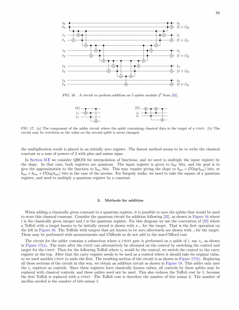
68

i0 • • • i0t0 • • (t+ i)0

• • • • •i1 • • • i1t1 • • (t+ i)1

• • • • •i2 • • • i2t2 • • (t+ i)2

• • • • •i3 • • • i3t3 • • (t+ i)3

•i4 • i4t4 (t+ i)4

FIG. 16. A circuit to perform addition on 5 qubits modulo 25 from [32].

(a) • •i1 •t1 •

(b) • •i1 • •t1 •

FIG. 17. (a) The component of the adder circuit where the qubit containing classical data is the target of a cnot. (b) Thecircuit may be rewritten so the value on the second qubit is never changed.

the multiplication result is placed in an initially zero register. The fastest method seems to be to write the classicalconstant as a sum of powers of 2 with plus and minus signs.

In Section II E we consider QROM for interpolation of functions, and we need to multiply the input register bythe slope. In that case, both registers are quantum. The input register is given to bdif bits, and the goal is togive the approximation to the function to bsm bits. This may require giving the slope to bsm + O(log bsm) bits, orbsm + bfun +O(log bsm) bits in the case of the arcsine. For Szegedy walks, we need to take the square of a quantumregister, and need to multiply a quantum register by a constant.

2. Methods for addition

When adding a classically given constant to a quantum register, it is possible to save the qubits that would be usedto store this classical constant. Consider the quantum circuit for addition following [32], as shown in Figure 16 wherei is the classically given integer and t is the quantum register. For this diagram we use the convention of [32] wherea Toffoli with a target known to be initially zeroed is shown with a x for the target. That is the first operation onthe left in Figure 16. The Toffolis with targets that are known to be zero afterwards are shown with y for the target.These may be performed with measurements and Cliffords so do not add to the non-Clifford cost.

The circuit for the adder contains a subsection where a cnot gate is performed on a qubit of i, say i1, as shownin Figure 17(a). The state after the cnot can alternatively be obtained on the control by switching the control andtarget for the cnot. Then for the following Toffoli where i1 would be the control, we switch the control to the carryregister at the top. After that the carry register needs to be used as a control where it should take its original value,so we need another cnot to undo the first. The resulting section of the circuit is as shown in Figure 17(b). Replacingall these sections of the circuit in this way, we obtain an addition circuit as shown in Figure 18. This adder only usesthe ij registers as controls. Since these registers have classically known values, all controls by these qubits may bereplaced with classical controls, and these qubits need not be used. This also reduces the Toffoli cost by 1, becausethe first Toffoli is replaced with a cnot. The Toffoli cost is therefore the number of bits minus 2. The number ofancillas needed is the number of bits minus 1.

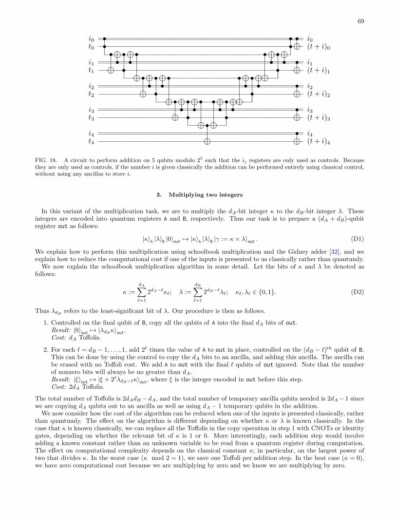
69

i0 • • • i0t0 • • (t+ i)0

• • • • •i1 • • • • • i1t1 • • (t+ i)1

• • • • •i2 • • • • • i2t2 • • (t+ i)2

• • • • •i3 • • • • • i3t3 • • (t+ i)3

•i4 • i4t4 (t+ i)4

FIG. 18. A circuit to perform addition on 5 qubits modulo 25 such that the ij registers are only used as controls. Becausethey are only used as controls, if the number i is given classically the addition can be performed entirely using classical control,without using any ancillas to store i.

3. Multiplying two integers

In this variant of the multiplication task, we are to multiply the dA-bit integer κ to the dB-bit integer λ. Theseintegers are encoded into quantum registers A and B, respectively. Thus our task is to prepare a (dA + dB)-qubitregister out as follows:

|κ〉A |λ〉B |0〉out 7→ |κ〉A |λ〉B |γ := κ× λ〉out . (D1)

We explain how to perform this multiplication using schoolbook multiplication and the Gidney adder [32], and weexplain how to reduce the computational cost if one of the inputs is presented to us classically rather than quantumly.

We now explain the schoolbook multiplication algorithm in some detail. Let the bits of κ and λ be denoted asfollows:

κ :=

dA∑`=1

2dA−`κ`; λ :=

dB∑`=1

2dB−`λ`; κ`, λ` ∈ 0, 1. (D2)

Thus λdB refers to the least-significant bit of λ. Our procedure is then as follows.

1. Controlled on the final qubit of B, copy all the qubits of A into the final dA bits of out.Result: |0〉out 7→ |λdBκ〉out.Cost: dA Toffolis.

2. For each ` = dB − 1, . . . , 1, add 2` times the value of A to out in place, controlled on the (dB − `)th qubit of B.This can be done by using the control to copy the dA bits to an ancilla, and adding this ancilla. The ancilla canbe erased with no Toffoli cost. We add A to out with the final ` qubits of out ignored. Note that the numberof nonzero bits will always be no greater than dA.Result: |ξ〉out 7→ |ξ + 2`λdB−`κ〉out, where ξ is the integer encoded in out before this step.Cost: 2dA Toffolis.

The total number of Toffolis is 2dAdB − dA, and the total number of temporary ancilla qubits needed is 2dA− 1 sincewe are copying dA qubits out to an ancilla as well as using dA − 1 temporary qubits in the addition.

We now consider how the cost of the algorithm can be reduced when one of the inputs is presented classically, ratherthan quantumly. The effect on the algorithm is different depending on whether κ or λ is known classically. In thecase that κ is known classically, we can replace all the Toffolis in the copy operation in step 1 with CNOTs or identitygates, depending on whether the relevant bit of κ is 1 or 0. More interestingly, each addition step would involveadding a known constant rather than an unknown variable to be read from a quantum register during computation.The effect on computational complexity depends on the classical constant κ; in particular, on the largest power oftwo that divides κ. In the worst case (κ mod 2 = 1), we save one Toffoli per addition step. In the best case (κ = 0),we have zero computational cost because we are multiplying by zero and we know we are multiplying by zero.

70

In the case that λ is presented to us classically rather than quantumly, we can make the addition controlled byperforming the (non-controlled) addition circuit in the case of 1, or doing nothing when the classical control is 0. Thenumber of quantum-to-quantum additions would thus depend on the number of non-zero classical bits – the greaterthe Hamming weight of the classical input, the greater the number of additions to be performed. Note that this isdistinct from the cost of performing classical-to-quantum multiplication when κ is the classical variable, in which casethe complexity is determined by the number of zeros on the far right of the number.

The case where λ is given classically is more relevant for this paper. We are unlikely to be dealing with classicallyspecified integers that are a multiple of a large power of two. On the other hand, we will frequently have someinformation about the Hamming weight

∑` λ` of the classically known number λ. Each addition costs at most dA

Toffolis, we perform∑` λ` ≤ dB such additions, and no other operations require Toffoli gates. We therefore have a

total Toffoli cost of at most dAdB , which can be replaced with dA∑` λ` if we can assume knowledge of the Hamming

weight of λ. Thus we save a factor of 2 if one of the inputs is classical.In the following subsections, we explain how to modify the above procedure for variants of the multiplication task.

These variants have at least one of the inputs being a real number between 0 and 1, rather than an integer. Thus thetask is not to calculate the multiplication exactly, as this would involve infinitely many bits for real numbers. Instead,we truncate the binary expansions of real numbers to ensure that an error threshold is achieved.

4. Multiplying an integer to a real number

Now we consider a variant of the multiplication task where one of the inputs is a real number between zero andone. For reasons that become clear below, we specify κ to be the real number and λ to be the integer. We assumethat the real number is defined to infinitely many digits and that our task is to approximate γ := κ× λ to within anerror tolerance ε. Thus our task is to calculate some γ such that |γ − γ| < ε. That is to say, we are to prepare a newquantum register out as follows:

|κ〉A |λ〉B |0〉out 7→ |κ〉A |λ〉B |γ〉out . (D3)

Here we are free to choose the number of bits for the register A and hence the number of bits for the register out.This choice will naturally depend on the error tolerance ε.

We begin by specifying symbols for the bits of the inputs κ and λ. Note that the indexing differs somewhat fromthe previous section. We define

κ :=

∞∑`=1

κ`/2`; λ :=

dB∑`=1

2dB−`λ`; κ`, λ` ∈ 0, 1. (D4)

We then select an integer dA ≥ dB (presuming ε < 1) that will count the number of bits of the input κ we plan touse. We use dA − 1 bits of κ. We explain our plan by first representing the ideal product as

γ =

λ1 × κ1 κ2 κ3 · · · κdB−2 κdB−1 . κdB · · · κdA−1 κdA · · ·+ λ2 × κ1 κ2 · · · κdB−3 κdB−2 . κdB−1 · · · κdA−2 κdA−1 · · ·+ λ3 × κ1 · · · κdB−4 κdB−3 . κdB−2 · · · κdA−3 κdA−2 · · ·

...

+ λdB−1 × κ1 . κ2 · · · κdA−dB+1 κdA−dB+2 · · ·+ λdB × 0 . κ1 · · · κdA−dB κdA−dB+1 · · ·

, (D5)

where the vertical line denotes where we truncate the binary expansion of κ. We thus calculate

γdA :=

dB∑`=1

λ`bκ2dA−`c2dB−dA ; γ − γdA ≤ dB2dB−dA . (D6)

To ensure that the error tolerance ε is achieved, we should choose dA > dB + log(dB/ε). We therefore choose

dA = dB + dlog(dB/ε)e. (D7)

We follow a similar strategy to that described in Appendix D 3, meaning that we are to perform a sequence ofcontrolled additions. We work bottom to top in Eq. (D5).

71

We start with the bottom line by copying dA − dB bits into the output register, with Toffoli cost dA − dB . Afterthat the number of Toffolis is twice the number of bits. The total number of Toffolis is then

(dA − dB) + 2(dA − dB + 1) + . . .+ 2(dA − 1) = dA − dB +

dA−1∑`=dA−dB+1

`

= dA(2dB − 1)− dB2

= (dB + dlog(dB/ε)e)(2dB − 1)− dB2

= dB2 + (2dB − 1)dlog(dB/ε)e − dB . (D8)

Hence the Toffoli cost of multiplying a real number to an integer on a quantum computer is no more than

dB2 + (2dB − 1)dlog(dB/ε)e − dB , (D9)

where dB is the number of bits used to specify the integer and ε is the allowable error in the overall multiplication.The algorithm requires that the real number is specified to dA = ddB log(dB/ε)e bits and uses dA − 1 ancilla qubits.

5. Multiplying two different real numbers

In this subsection we consider the task where we are to multiply two real numbers κ (0 ≤ κ < 1) and λ (0 ≤ κ < 1).Our task is to calculate an approximation γ to γ := κ × λ such that |γ − γ| < ε, where ε > 0 is some given errortolerance. That is to say, we are to prepare a new quantum register out as follows:

|κ〉A |λ〉B |0〉out 7→ |κ〉A |λ〉B |γ〉out . (D10)

We are free to choose the number of qubits in each of the registers A, B, and out to ensure that the output encodes avalue for γ that approximates γ to within the error tolerance ε. We begin by discussing these choices of register size,starting with the size of A and B.

To explain our choice for the numbers of qubits for registers A and B, we begin by introducing notation for theinputs κ and λ. As before, we define the bits of the inputs according to the equations

κ :=

∞∑`=1

κ`/2`; λ :=

∞∑`=1

λ`/2`; κ`, λ` ∈ 0, 1. (D11)

This suggests our strategy for calculating γ. As before, we have

γ =

λ1 × .0 κ1 κ2 κ3 · · · κdB−2 κdB−1 κdB · · · κdA−1 κdA · · ·+ λ2 × .0 0 κ1 κ2 · · · κdB−3 κdB−2 κdB−1 · · · κdA−2 κdA−1 · · ·+ λ3 × .0 0 0 κ1 · · · κdB−4 κdB−3 κdB−2 · · · κdA−3 κdA−2 · · ·

...

+ λdB−1 × .0 0 0 0 · · · 0 κ1 κ2 · · · κdA−dB+1 κdA−dB · · ·+ λdB × .0 0 0 0 · · · 0 0 κ1 · · · κdA−dB κdA−dB−1 · · ·

...

, (D12)

where solid lines indicate where we truncate the calculation in order to produce the approximation γ instead of γ.Here we have assumed that dA ≥ dB ; if dA < dB , our repeated addition procedure would involve several additions byzero. The repeated addition strategy has a Toffoli cost of

(dA − dB + 1) + 2(dA − dB + 2) + . . .+ 2(dA − 1) = (dA − dB + 1) + 2

dA−1∑`=dA−dB+2

`

= dA(2dB − 3)− (dB − 1)2. (D13)

It seems reasonable to set dA = dB , and numerical evidence indicates that this choice makes the optimal tradeoffbetween computational complexity and error tolerance. Setting d := dA = dB , the Toffoli cost is simply d2 − d− 1.

72

10 6 10 5 10 4 10 3 10 2 10 1

0.65

0.70

0.75

0.80

0.85

0.90

0.95

1.00

(d+

1)/(2

d)

Justifying no. bits for truncated multiplication

FIG. 19. Numerical justification for our choice of d in Eq. (D17). We plot the ratio of (d+ 1)/2d to the error bound ε. A valueless than 1 ensures that our choice of d yields a multiplication result whose error is less than ε.

We now consider the error of the sum in Eq. (D12). There

γ =

∞∑n,m=1n+m≤d

κnλm2−(n+m), (D14)

so

γ − γ =

∞∑n,m=1n+m>d

κnλm2−(n+m) ≤∞∑

n,m=1n+m>d

2−(n+m) =d+ 1

2d. (D15)

We can ensure that the error of the approximation γ is within tolerance ε by setting

d+ 1

2d≤ ε. (D16)

Though the above could be solved exactly using a Lambert-W function, it is satisfied with

d = 1 + log(1/ε) + log(1 + log(1/ε)). (D17)

Figure 19 justifies this choice by depicting the value of d+12dε

as a function of ε with d chosen as per Eq. (D17). Tochoose d, we take the ceiling of this expression, because d must be chosen to be an integer.

Hence our strategy for multiplying two real numbers uses

d2 − d− 1 = log2(1/ε) + 2 log(1/ε) log log(1/ε) +O(log(1/ε)) (D18)

Toffoli gates to achieve an output with error less than ε. The ancilla cost is d− 1 bits for a copy of the bits of κ forthe controlled addition, and another d− 1 bits for the addition itself. Thus the ancilla cost is

2 log(1/ε) +O(log log(1/ε)). (D19)

6. Squaring a real number

We are given a quantum register A with a real number κ that satisfies 0 ≤ κ < 1. Our task is to calculate anapproximation γ of γ := κ2 such that |γ − γ| < ε, where ε is given (0 < ε < 1). That is to say, we are to prepare anew quantum register out as follows:

|κ〉A |0〉out 7→ |κ〉A |γ〉out . (D20)

73

We will include d bits in the sum, so the sum can be expressed as

γ =

∞∑n,m=1n+m≤d

κnκm2−(n+m). (D21)

We take advantage of symmetry to rewrite the sum as

γ = 2

∞∑n,m=1

n+m≤d,n>m

κnκm2−(n+m) +

bd/2c∑n=1

κn2−2n

= 2

d−1∑n=1

κn

min(n−1,d−n)∑m=1

κm2−(n+m) +

bd/2c∑n=1

κn2−2n. (D22)

The first term in this sum contains the parts where n > m, and is multiplied by 2 because those parts with n < mare equal by symmetry. The second term is that for n = m. This sum is more efficient, because only about half asmany terms appear. Now the term in the second sum for n = bd/2c is half the size of any of the other terms, so it isconvenient to omit it.

The form of the sum can be shown, for the odd example d = 15,

γ =

κ1 × .0 κ1 0 0 0 0 0 0 0 0 0 0 0 0

+ κ2 × .0 κ1 0 κ2 0 0 0 0 0 0 0 0 0 0

+ κ3 × .0 0 κ1 κ2 0 κ3 0 0 0 0 0 0 0 0

+ κ4 × .0 0 0 κ1 κ2 κ3 0 κ4 0 0 0 0 0 0

+ κ5 × .0 0 0 0 κ1 κ2 κ3 κ4 0 κ5 0 0 0 0

+ κ6 × .0 0 0 0 0 κ1 κ2 κ3 κ4 κ5 0 κ6 0 0

+ κ7 × .0 0 0 0 0 0 κ1 κ2 κ3 κ4 κ5 κ6 0 κ7

+ κ8 × .0 0 0 0 0 0 0 κ1 κ2 κ3 κ4 κ5 κ6 κ7

+ κ9 × .0 0 0 0 0 0 0 0 κ1 κ2 κ3 κ4 κ5 κ6

+ κ10 × .0 0 0 0 0 0 0 0 0 κ1 κ2 κ3 κ4 κ5

+ κ11 × .0 0 0 0 0 0 0 0 0 0 κ1 κ2 κ3 κ4

+ κ12 × .0 0 0 0 0 0 0 0 0 0 0 κ1 κ2 κ3

+ κ13 × .0 0 0 0 0 0 0 0 0 0 0 0 κ1 κ2

+ κ14 × .0 0 0 0 0 0 0 0 0 0 0 0 0 κ1

. (D23)

Here we have shown terms from the second sum from Eq. (D22) in blue. In the case where d is odd, bd/2c = (d−1)/2,and we can write the sum as

γ =

(d−1)/2∑n=1

κn

(2−2n + 2

n−1∑m=1

κnκm2−(n+m)

)+ 2

d−1∑n=(d+1)/2

κn

d−n∑m=1

κm2−(n+m). (D24)

The first sum in Eq. (D24) corresponds to the part above the horizontal line in Eq. (D23), and the second sum inEq. (D24) corresponds to the part below the line. To compute Eq. (D24), we start at the least significant digit, andmove to the most significant digit (corresponding to moving from the bottom row to the top row in Eq. (D29)), as

γ =

(d+1)/2∑n=d−1

κn

d−n∑m=1

κm2−(n+m−1) +

1∑n=(d−1)/2

κn

(2−2n +

n−1∑m=1

κnκm2−(n+m−1)

). (D25)

To compute the sum we start with n = d−1, and copy the value κd−1κ1 into the output at position d−1 (to initializethe output as κd−1κ12−(d−1)) with Toffoli cost 1. Next, we use κd−2 to control addition of κ12−(d−2) +κ22−(d−1) intothe output. This controlled addition has cost 2× 2 because it is for 2 bits. At step j = d− n ≤ (d− 1)/2, the cost ofcontrolled addition of j bits is 2j. The cost of that part is therefore

1 +

(d−1)/2∑j=2

2j = (d2 − 5)/4. (D26)

74

For the remaining steps with n = (d − 1)/2 to 2, we have a cost of n − 1 to produce the n − 1 values of κnκm, andthere are n+ 1 bits that need to be added into the output. That includes the bit for κn2−2n which is spaced by onebit from the remaining bits for κnκm. That gives cost (n− 1) + (n+ 1) = 2n. For n = 1, we just have a cost of oneToffoli to add in the single bit (without a control, because it is just κn). That gives the same cost as the first half,for a total cost of

d2/2− 5/2. (D27)

In the case where d is even, bd/2c = d/2, and we can write the sum as

γ =

d/2−1∑n=1

κn

(2−2n + 2

n−1∑m=1

κnκm2−(n+m)

)+ 2κd/2

d/2−1∑m=1

κm2−(d/2+m) + 2

d∑n=d/2+1

κn

d+1−n∑m=1

κm2−(n+m). (D28)

The form of the sum for an even example d = 16 is

γ =

κ1 × .0 κ1 0 0 0 0 0 0 0 0 0 0 0 0 0

+ κ2 × .0 κ1 0 κ2 0 0 0 0 0 0 0 0 0 0 0

+ κ3 × .0 0 κ1 κ2 0 κ3 0 0 0 0 0 0 0 0 0

+ κ4 × .0 0 0 κ1 κ2 κ3 0 κ4 0 0 0 0 0 0 0

+ κ5 × .0 0 0 0 κ1 κ2 κ3 κ4 0 κ5 0 0 0 0 0

+ κ6 × .0 0 0 0 0 κ1 κ2 κ3 κ4 κ5 0 κ6 0 0 0

+ κ7 × .0 0 0 0 0 0 κ1 κ2 κ3 κ4 κ5 κ6 0 κ7 0

+ κ8 × .0 0 0 0 0 0 0 κ1 κ2 κ3 κ4 κ5 κ6 κ7 0

+ κ9 × .0 0 0 0 0 0 0 0 κ1 κ2 κ3 κ4 κ5 κ6 κ7

+ κ10 × .0 0 0 0 0 0 0 0 0 κ1 κ2 κ3 κ4 κ5 κ6

+ κ11 × .0 0 0 0 0 0 0 0 0 0 κ1 κ2 κ3 κ4 κ5

+ κ12 × .0 0 0 0 0 0 0 0 0 0 0 κ1 κ2 κ3 κ4

+ κ13 × .0 0 0 0 0 0 0 0 0 0 0 0 κ1 κ2 κ3

+ κ14 × .0 0 0 0 0 0 0 0 0 0 0 0 0 κ1 κ2

+ κ15 × .0 0 0 0 0 0 0 0 0 0 0 0 0 0 κ1

. (D29)

Again we have shown terms from the second sum from Eq. (D22) in blue. The first sum in Eq. (D28) corresponds tothe part above the first horizontal line in Eq. (D29), the second sum in Eq. (D28) corresponds to the part betweenthe two lines in Eq. (D29), and the third sum in Eq. (D28) corresponds to the part below the second horizontal linein Eq. (D29). To compute Eq. (D28), we again start at the least significant digit, and move to the most significantdigit, as

γ =

d/2+1∑n=d

κn

d+1−n∑m=1

κm2−(n+m−1) + κd/2

d/2−1∑m=1

κm2−(d/2+m−1) +

1∑n=d/2−1

κn

(2−2n +

n−1∑m=1

κnκm2−(n+m−1)

). (D30)

For the costing of the additions, we have the same costing for the first sum in Eq. (D30) as in the odd case, givingcost

1 +

d/2−1∑j=2

2j = (d2 − 2d− 4)/4. (D31)

The middle sum in Eq. (D30) has cost d− 2, then the final sum has cost 2n for n = 2 to d/2− 1, and cost 1 for n = 1,giving the same cost as the first sum. That gives a total complexity

d2/2− 4. (D32)

Thus in both the odd and even cases the complexity is less than d2/2.

75

To estimate the error, we have

γ − γ = 2

∞∑n,m=1

n+m>d,n>m

κnκm2−(n+m) +

∞∑n=bd/2c

κn2−2n

≤ 2

∞∑n,m=1

n+m>d,n>m

2−(n+m) +

∞∑n=bd/2c

2−2n

=

∞∑`=d+1

b(`− 1)/2c2−` +4

32−2bd/2c. (D33)

In the case of even d we get

1

2d 2−d +

1

32−d +

4

32−d =

1

2d 2−d +

5

32−d, (D34)

and in the case of odd d we get

1

2d 2−d +

1

62−d +

8

32−d =

1

2d 2−d +

17

62−d. (D35)

We find that we can limit the error to ε using

d = dlog(1/ε) + log(11/3 + log(1/ε))e. (D36)

The Toffoli cost of squaring is then (regardless of whether d is odd or even)

d2/2 =1

2log2(1/ε) + log(1/ε) log log(1/ε) +O(log(1/ε)). (D37)

The ancilla cost in the case where d is even has a maximum of d − 2. When n = d/2 (corresponding to the partbetween the two horizontal lines in Eq. (D29)), there are d/2− 1 bits to add in a controlled way, so there are d/2− 1bits for the copy and another d/2− 1 bits for the addition itself. When n = d/2− 1, there are d/2− 2 bits to add ina controlled way, and a range of d/2 bits to add in which give an ancilla cost of d/2. In both these cases, the ancillacost is d − 2. When d is odd, the ancilla cost is d − 1. When n = dd/2e (the part just below the horizontal line inEq. (D23)), there are dd/2e − 1 bits to add in a controlled way, which takes 2(dd/2e − 1) = d− 1 ancillas for d odd.When n = dd/2e − 1, there are dd/2e − 2 bits to add in a controlled way, and a range of dd/2e bits to add, for a totalancilla cost of d− 1. Hence the ancilla cost of squaring is only half that for multiplication, and is

log(1/ε) +O(log log(1/ε)). (D38)

Appendix E: Other approaches to Hamiltonian evolution based optimization

Here we outline two other approaches in the literature to optimization based on Hamiltonian evolution. We consider“shortest path” optimization in Appendix E 1 and we consider quantum-enhanced population transfer in Appendix E 2.In both cases, we review the techniques and explain how the algorithmic primitives we develop in this paper could beapplied in each approach.

1. Heuristic variant of the shortest path algorithm

Hastings’ “shortest path algorithm” [9] (SPA) is an interesting approach to quantum optimization that is also basedon time evolution under a cost function with some non-commuting driver Hamiltonian. Perhaps the most intriguingproperty of the SPA is that Hastings was able to rigorously show that the SPA gives a super-Grover (i.e., betterthan quadratic) speedup for certain classical optimization problems – e.g., for an arbitrary instance of the problemMAX-2-LIN2 (which is a problem very closely related to QUBO) [75]. The results of [9] and [75] also rigorously (andin some cases, empirically) show similar speedups under a variety of assumptions about related problems.

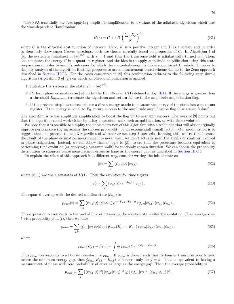
76

The SPA essentially involves applying amplitude amplification to a variant of the adiabatic algorithm which usesthe time-dependent Hamiltonian

H(s) = C + sB

(∑pXp

N

)K(E1)

where C is the diagonal cost function of interest. Here, K is a positive integer and B is a scalar, and in orderto rigorously show super-Grover speedups, both are chosen carefully based on properties of C. In Algorithm 1 of

[9], the system is initialized in |+〉⊗N with s = 1 and then the transverse field is adiabatically turned off. Then,one computes the energy C in a quantum register, and the idea is to apply amplitude amplification using this statepreparation in order to amplify outcomes for which the computed energy is below some target threshold. In order tosimplify analysis of the algorithm Hastings proposes to use a measurement based scheme similar to the Zeno approachdescribed in Section III C 3. For the cases considered in [9] this combination reduces to the following very simplealgorithm (Algorithm 3 of [9]) on which amplitude amplification is applied:

1. Initialize the system in the state |ψ〉 = |+〉⊗N .

2. Perform phase estimation on |ψ〉 under the Hamiltonian H(1) defined in Eq. (E1). If the energy is greater thana threshold Ethreshold, terminate the algorithm and return failure to the amplitude amplification flag.

3. If the previous step has succeeded, use a direct energy oracle to measure the energy of the state into a quantumregister. If the energy is equal to E0, return success to the amplitude amplification flag (else return failure).

The algorithm is to use amplitude amplification to boost the flag bit to near unit success. The work of [9] points outthat the algorithm could work either by using a quantum walk such as qubitization, or with time evolution.

We note that it is possible to simplify the implementation of this algorithm with a technique that will also marginallyimprove performance (by increasing the success probability by an exponentially small factor). Our modification is tosuggest that one proceed to step 3 regardless of whether or not step 2 succeeds. In doing this, we see that becausethe result of the phase estimation measurement is never used, we don’t actually need the ancilla or controls involvedin phase estimation. Instead, we can follow similar logic to [21] to see that the procedure becomes equivalent toperforming time evolution (or applying a quantum walk) for randomly chosen duration. We can choose the probabilitydistribution to suppress phase measurement errors as large as the energy gap, as described in Section III C 3.

To explain the effect of this approach in a different way, consider writing the initial state as

|ψ〉 =∑j

〈ψj,1|ψ〉 |ψj,1〉 , (E2)

where |ψj,1〉 are the eigenstates of H(1). Then the evolution for time t gives

|ψ〉 =∑j

〈ψj,1|ψ〉 e−iEj,1t |ψj,1〉 . (E3)

The squared overlap with the desired solution state |ψ0,0〉 is

psucc(t) =∑j,k

〈ψj,1|ψ〉 〈ψ|ψk,1〉 e−i(Ej,1−Ek,1)t 〈ψ0,0|ψj,1〉 〈ψk,1|ψ0,0〉 . (E4)

This expression corresponds to the probability of measuring the solution state after the evolution. If we average overt with probability ptime(t), then we have

psucc =∑j,k

〈ψj,1|ψ〉 〈ψ|ψk,1〉 ptime(Ej,1 − Ek,1) 〈ψ0,0|ψj,1〉 〈ψk,1|ψ0,0〉 , (E5)

where

ptime(Ej,1 − Ek,1) =

∫dt ptime(t)e−i(Ej,1−Ek,1)t. (E6)

Thus ptime corresponds to a Fourier transform of ptime. If ptime is chosen such that its Fourier transform goes to zerobefore the minimum energy gap, then ptime(Ej,1 − Ek,1) is nonzero only for j = k. That is equivalent to having ameasurement of phase with zero probability of error as large as the energy gap. Then the average probability is

psucc =∑j

| 〈ψj,1|ψ〉 |2| 〈ψ0,0|ψj,1〉 |2 ≥ | 〈ψ0,1|ψ〉 |2| 〈ψ0,0|ψ0,1〉 |2. (E7)

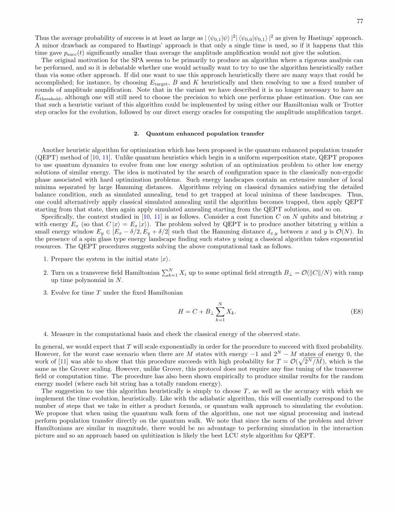
77

Thus the average probability of success is at least as large as | 〈ψ0,1|ψ〉 |2| 〈ψ0,0|ψ0,1〉 |2 as given by Hastings’ approach.A minor drawback as compared to Hastings’ approach is that only a single time is used, so if it happens that thistime gave psucc(t) significantly smaller than average the amplitude amplification would not give the solution.

The original motivation for the SPA seems to be primarily to produce an algorithm where a rigorous analysis canbe performed, and so it is debatable whether one would actually want to try to use the algorithm heuristically ratherthan via some other approach. If did one want to use this approach heuristically there are many ways that could beaccomplished; for instance, by choosing Etarget, B and K heuristically and then resolving to use a fixed number ofrounds of amplitude amplification. Note that in the variant we have described it is no longer necessary to have anEthreshold, although one will still need to choose the precision to which one performs phase estimation. One can seethat such a heuristic variant of this algorithm could be implemented by using either our Hamiltonian walk or Trotterstep oracles for the evolution, followed by our direct energy oracles for computing the amplitude amplification target.

2. Quantum enhanced population transfer

Another heuristic algorithm for optimization which has been proposed is the quantum enhanced population transfer(QEPT) method of [10, 11]. Unlike quantum heuristics which begin in a uniform superposition state, QEPT proposesto use quantum dynamics to evolve from one low energy solution of an optimization problem to other low energysolutions of similar energy. The idea is motivated by the search of configuration space in the classically non-ergodicphase associated with hard optimization problems. Such energy landscapes contain an extensive number of localminima separated by large Hamming distances. Algorithms relying on classical dynamics satisfying the detailedbalance condition, such as simulated annealing, tend to get trapped at local minima of these landscapes. Thus,one could alternatively apply classical simulated annealing until the algorithm becomes trapped, then apply QEPTstarting from that state, then again apply simulated annealing starting from the QEPT solutions, and so on.

Specifically, the context studied in [10, 11] is as follows. Consider a cost function C on N qubits and bitstring xwith energy Ex (so that C |x〉 = Ex |x〉). The problem solved by QEPT is to produce another bitstring y within asmall energy window Ey ∈ [Ex − δ/2, Ey + δ/2] such that the Hamming distance dx,y between x and y is O(N). Inthe presence of a spin glass type energy landscape finding such states y using a classical algorithm takes exponentialresources. The QEPT procedures suggests solving the above computational task as follows.

1. Prepare the system in the initial state |x〉.

2. Turn on a transverse field Hamiltonian∑Nk=1Xi up to some optimal field strength B⊥ = O(‖C‖/N) with ramp

up time polynomial in N .

3. Evolve for time T under the fixed Hamiltonian

H = C +B⊥

N∑k=1

Xk. (E8)

4. Measure in the computational basis and check the classical energy of the observed state.

In general, we would expect that T will scale exponentially in order for the procedure to succeed with fixed probability.However, for the worst case scenario when there are M states with energy −1 and 2N −M states of energy 0, thework of [11] was able to show that this procedure succeeds with high probability for T = O(

√2N/M), which is the

same as the Grover scaling. However, unlike Grover, this protocol does not require any fine tuning of the transversefield or computation time. The procedure has also been shown empirically to produce similar results for the randomenergy model (where each bit string has a totally random energy).

The suggestion to use this algorithm heuristically is simply to choose T , as well as the accuracy with which weimplement the time evolution, heuristically. Like with the adiabatic algorithm, this will essentially correspond to thenumber of steps that we take in either a product formula, or quantum walk approach to simulating the evolution.We propose that when using the quantum walk form of the algorithm, one not use signal processing and insteadperform population transfer directly on the quantum walk. We note that since the norm of the problem and driverHamiltonians are similar in magnitude, there would be no advantage to performing simulation in the interactionpicture and so an approach based on qubitization is likely the best LCU style algorithm for QEPT.