Competitive Food Supply Chain Networks with Application to ... · Competitive Food Supply Chain...
30
Competitive Food Supply Chain Networks with Application to Fresh Produce Min Yu Department of Finance and Operations Management Isenberg School of Management University of Massachusetts, Amherst, Massachusetts 01003 Anna Nagurney * Department of Finance and Operations Management Isenberg School of Management University of Massachusetts, Amherst, Massachusetts 01003 and School of Business, Economics and Law University of Gothenburg, Gothenburg, Sweden March 2012; revised July 2012 European Journal of Operational Research 224(2) (2013) pp 273-282. Abstract: In this paper, we develop a network-based food supply chain model under oligopolistic competition and perishability, with a focus on fresh produce. The model in- corporates food deterioration through the introduction of arc multipliers, with the inclusion of the discarding costs associated with the disposal of the spoiled food products. We allow for product differentiation due to product freshness and food safety concerns, as well as the evaluation of alternative technologies associated with various supply chain activities. We then propose an algorithm with elegant features for computation. A case study focused on the cantaloupe market is investigated within this modeling and computational framework, in which we analyze different scenarios prior/during/after a foodborne disease outbreak. Key words: food supply chains, fresh produce, oligopolistic competition, food deterioration, product differentiation * Corresponding Author; e-mail: [email protected]; phone: 413-545-5635; fax: 413-545-3858 1
Transcript of Competitive Food Supply Chain Networks with Application to ... · Competitive Food Supply Chain...
Competitive Food Supply Chain Networks
with
Application to Fresh Produce
Min Yu
Department of Finance and Operations Management
Isenberg School of Management
University of Massachusetts, Amherst, Massachusetts 01003
Anna Nagurney∗
Department of Finance and Operations Management
Isenberg School of Management
University of Massachusetts, Amherst, Massachusetts 01003
and
School of Business, Economics and Law
University of Gothenburg, Gothenburg, Sweden
March 2012; revised July 2012
European Journal of Operational Research 224(2) (2013) pp 273-282.
Abstract: In this paper, we develop a network-based food supply chain model under
oligopolistic competition and perishability, with a focus on fresh produce. The model in-
corporates food deterioration through the introduction of arc multipliers, with the inclusion
of the discarding costs associated with the disposal of the spoiled food products. We allow
for product differentiation due to product freshness and food safety concerns, as well as the
evaluation of alternative technologies associated with various supply chain activities. We
then propose an algorithm with elegant features for computation. A case study focused on
the cantaloupe market is investigated within this modeling and computational framework,
in which we analyze different scenarios prior/during/after a foodborne disease outbreak.
Key words: food supply chains, fresh produce, oligopolistic competition, food deterioration,
product differentiation
∗ Corresponding Author; e-mail: [email protected]; phone: 413-545-5635; fax:
413-545-3858
1
1. Introduction
Today, food supply chains are complex, global networks, creating pathways from farms to
consumers, involving production, processing, distribution, and even the disposal of food (see
Boehlje (1999), van der Vorst (2000), Aramyan et al. (2006), Monteiro (2007), Trienekens
and Zuurbier (2008), and Ahumada and Villalobos (2009)). Consumers’ expectation of year-
around availability of fresh food products has encouraged the globalization of food markets
(see Cook (2002), Monteiro (2007), Trienekens and Zuurbier (2008), and Ahumada and Vil-
lalobos (2009)). For instance, the United States is ranked number one as both importer and
exporter in the international trade of horticultural commodities, accounting for about 18% of
the $44 billion global horticultural trade even a decade ago (Cook (2002)). In the US alone,
consumers now spend over 1.6 trillion dollars annually on food (Plunkett Research (2011)).
With growing global competition (Ahumada and Villalobos (2009)), coupled with the as-
sociated greater distances between food production and consumption locations (Monteiro
(2007)), there is increasing pressure for the integration of food production and distribution
along the chain (Boehlje (1999) and Cook (2002)) and, hence, new challenges for food supply
chain modeling and management, analysis, and solutions.
Food supply chains are distinct from other product supply chains. The fundamental
difference between food supply chains and other supply chains is the continuous and signif-
icant change in the quality of food products throughout the entire supply chain until the
points of final consumption (see Sloof, Tijskens, and Wilkinson (1996), van der Vorst (2000),
Lowe and Preckel (2004), Ahumada and Villalobos (2009), Blackburn and Scudder (2009),
Akkerman, Farahani, and Grunow (2010), and Aiello, La Scalia, and Micale (2012)). This
is especially the case for fresh produce supply chains with increasing attention being placed
on both freshness and safety. Clearly, many consumers prefer the freshest produce at a fair
price (Cook (2002), Wilcock et al. (2004), and Lutke Entrup et al. (2005)). Moreover,
statistics from the United States Department of Agriculture (USDA (2011)) suggest that
the consumption of fresh vegetables has increased at a much faster pace than the demand
for traditional crops such as wheat and other grains.
Given the thin profit margins in the food industries, product differentiation strategies are
increasingly used in food markets (Lowe and Preckel (2004), Lusk and Hudson (2004), and
Ahumada and Villalobos (2009)) with product freshness considered one of the differentiating
factors (Karkkainen (2003) and Lutke Entrup et al. (2005)) and with a successful example
being fresh-cut produce, including bagged salads, washed baby carrots, and fresh-cut melons
(Cook (2002)). Retailers, such as Globus, a German retailer, are also now realizing that food
freshness can be a competitive advantage (Lutke Entrup et al. (2005); see also Aiello, La
2
Scalia, and Micale (2012)).
Moreover, the high perishability of food products has resulted in immense food waste/loss,
further stressing food supply chains and the associated quality and profitability. Some food
wastage and losses are inevitable in food supply chain network links (Thompson (2002),
Widodo et al. (2006), and Gustavsson et al. (2011)). However, it is estimated that approxi-
mately one third of the global food production is wasted or lost annually (Gustavsson et al.
(2011)). In any country, 20% – 60% of the total amount of agricultural fresh products has
been wasted or lost (Widodo et al. (2006)). Food products often require special handling,
transportation, and storage technologies (Zhang, Habenicht, and Spieß (2003), Lowe and
Preckel (2004), Trienekens and Zuurbier (2008), and Rong, Akkerman, and Grunow (2011)).
Furthermore, the quality of food products is decreasing with time, even with the utilization
of the most advanced facilities and conditions (Sloof, Tijskens, and Wilkinson (1996) and
Zhang, Habenicht, and Spieß (2003)).
Such challenges have underlined the need for the efficient management of food supply
chains, which is critical to profitability. Therefore, food supply chains have been receiving
increasing attention. Nahmias (1982, 2011) and Silver, Pyke, and Peterson (1998) provided
extensive reviews of the inventory management of perishable products. The reviews by Glen
(1987) and Lowe and Preckel (2004) focused on farm planning. In addition, Lutke En-
trup (2005) discussed thoroughly how to integrate shelf life into production planning within
three sample food industries (yogurt, sausages, and poultry). Akkerman, Farahani, and
Grunow (2010) outlined quantitative operations management applications in food distribu-
tion management. The survey by Lucas and Chhajed (2004) presented applications related
to location problems in agriculture and recognized the challenges of strategic production-
distribution planning problems in the agricultural industry. Due to the added complexity
caused by food perishability, there are fewer articles related to perishable food products than
those related to non-perishable ones, and even fewer models developed for fully integrated
supply chain system approaches (Ahumada and Villalobos (2009)), which is the focus of this
paper.
We now describe some of the contributions in the literature, which aim to integrate and
synthesize two or more processes associated with food supply chains. Zhang, Habenicht, and
Spieß (2003) studied a physical distribution system in order to minimize the total cost for
storage and shipment with the product quality requirement fulfilled. Widodo et al. (2006)
developed mathematical models dealing with flowering-harvesting and harvesting-delivering
problems of agricultural fresh products by introducing a plant maturing curve and a loss
function to address, respectively, the growing process and the decaying process of the fresh
3
products. Ahumada and Villalobos (2011) discussed the packing and distribution problem of
fresh produce, with the inclusion of perishability. They handled the perishability of the crops
through storage constraints, and used a loss function in the objective function. In addition,
Kopanos, Puigjaner, and Georgiadis (2012) studied the production-distribution planning
problem of a multisite, multiproduct, semicontinuous food processing industry within the
framework of mixed integer programming.
As noted by van der Vorst (2006), it is imperative to analyze food supply chains within
the context of the full complexity of their network structure. Monteiro (2007) claimed that
the theory of network economics (cf. Nagurney (1999)) provides a powerful mathematical
framework in which the supply chain can be graphically represented and analyzed. He further
adopted the theory of network economics to study the economics of traceability in food supply
chains theoretically. Blackburn and Scudder (2009) suggested a cost minimization model for
specific perishable product supply chain design, capturing the declining value of the product
over time. They noticed that product value deteriorates significantly over time at rates that
highly depend on temperature and humidity. Rong, Akkerman, and Grunow (2011), in turn,
presented a mixed integer linear programming model for the planning of food production
and distribution with a focus on product quality, which is strongly related to temperature
control throughout the supply chain.
Liu and Nagurney (2012) developed a multiperiod supply chain network equilibrium
model. That model can address perishability of products through changes in the underlying
network topologies. Nagurney and Aronson (1989), Masoumi, Yu, and Nagurney (2012),
Nagurney, Masoumi, and Yu (2012), Nagurney and Masoumi (2012), and Nagurney and
Nagurney (2012) have adopted arc multipliers to capture the perishability/waste of prod-
uct flows in a network. The latter three studies developed a system-optimization approach
from a single firm/organization’s perspective. Nagurney and Aronson (1989) constructed
a general dynamic spatial price equilibrium model, which can handle perishable products
through the use of arc multipliers. Masoumi, Yu, and Nagurney (2012) studied a generalized
oligopoly model with particular relevance to the pharmaceutical industry.
In this paper, we study the food supply chain management problem from a network
perspective, with the inclusion of food deterioration. We focus on fresh produce items, such
as vegetables and fruits, with simple or limited required processing, whose life cycle can be
measured in days. The fresh produce supply chain network oligopoly model developed in
this paper is distinct from other studies on perishable food products in several ways:
1. We capture the deterioration of fresh food along the entire supply chain from a network
4
perspective;
2. We handle the exponential time decay through the introduction of arc multipliers (more
details are given in Section 2 as to how to determine the arc multipliers);
3. We study oligopolistic competition with product differentiation;
4. We include the disposal of the spoiled food products, along with the associated costs;
5. We allow for the assessment of alternative technologies involved in each supply chain
activity.
We emphasize that with appropriate modifications, the model will be also applicable to
supply chain management of other perishable products under oligopolistic competition, and
even with quality competition.
This paper is organized as follows. In Section 2, we develop the new fresh produce
supply chain network oligopoly model and derive variational inequality formulations. We also
provide some qualitative properties. In Section 3, we present the computational algorithm,
which we then apply to a case study focused on fresh produce in the case of cantaloupes in
Section 4. We summarize our results and present our conclusions in Section 5.
2. The Fresh Produce Supply Chain Network Oligopoly Model
In this Section, we consider a finite number of I food firms, with a typical firm denoted
by i. The food supply chain network activities include the production, processing, storage,
distribution, and disposal of the food products. The food firms compete noncooperatively in
an oligopolistic manner. We allow for product differentiation by consumers at the demand
markets, due to product freshness and food safety concerns that may be associated with a
particular firm. In other words, the fresh food products are not necessarily homogeneous.
Each firm seeks to determine its optimal product flows throughout its entire supply chain
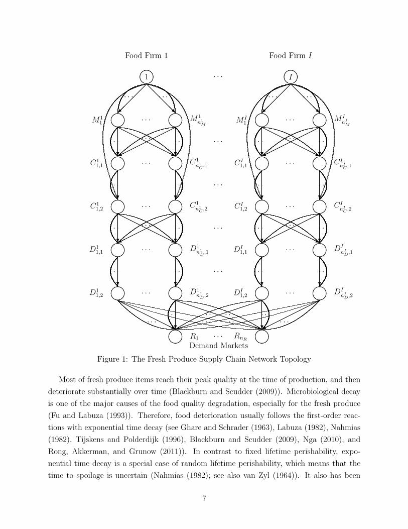
network by using Figure 1 as a schematic.
Each food firm is represented as a network of its economic activities. Each food firm i;
i = 1, . . . , I possesses niM production facilities, ni
C processors, and niD distribution centers,
in order to satisfy the demands at nR demand markets. Let G = [N, L] denote the graph
consisting of the set of nodes N and the set of links L in Figure 1; and L ≡ ∪i=1,...,ILi, where
Li denotes the set of directed links corresponding to the sequence of activities associated
with firm i.
5
The first set of links connecting the top two tiers of nodes corresponds to the food produc-
tion at each of the production units of firm i; i = 1, . . . , I, which may involve such a sequence
of seasonal operations as soil agitation, sowing, pest control, nutrient and water manage-
ment, and harvesting. The multiple possible links connecting each top tier node i with its
production facilities, M i1, . . . ,M
ini
M, capture different possible production technologies that
may be associated with a given facility.
The second set of links from the production facility nodes is connected to the processors of
each firm i; i = 1, . . . , I, which are denoted by Ci1,1, . . . , C
ini
C ,1. These links correspond to the
shipment links between the production units and the processors. The alternative shipment
links denote different possible modes of transportation, which represent the varying time
durations and environmental conditions associated with the shipment links.
The third set of links connecting nodes Ci1,1, . . . , C
ini
C ,1to Ci
1,2, . . . , Cini
C ,2; i = 1, . . . , I
denotes the processing of fresh produce. In this paper, the major food processing activities
are cleaning, sorting, labeling, and simple packaging. Different processing technologies may
result in dissimilar levels of quality degradation associated with the processing activities.
The next set of nodes represents the distribution centers, and, thus, the fourth set of links
connecting the processor nodes to the distribution centers is the set of shipment links. Such
distribution nodes associated with firm i; i = 1, . . . , I are denoted by Di1,1, . . . , D
ini
D,1. There
are also multiple shipment links, in order to capture different modes of transportation.
The fifth set of links, in turn, connects nodes Di1,1, . . . , D
ini
D,1to Di
1,2, . . . , Dini
D,2; i =
1, . . . , I, which represents the storage links. Since fresh produce items may require different
storage conditions, we represent these alternatives through multiple links at this tier.
The last set of links connecting the two bottom tiers of the supply chain network cor-
responds to distribution links over which the stored fresh produce items are shipped from
the distribution centers to the demand markets. Here we also allow for multiple modes of
transportation.
In addition, the curved links joining the top-tiered nodes i with the processors, which
are denoted by Ci1,2, . . . , C
ini
C ,2; i = 1, . . . , I, capture the possibility of on-site production and
processing.
6
����R1 · · · RnR
Demand Markets����
HHHHH
HHHHj
PPPPPPPPPPPPPPq?
��������������) ?
������
����· · · · · ·
· · · · · ·· · · · · ·· · · · · ·
D11,2 ����
· · · ����D1
n1D,2 DI
1,2 ����· · · ����
DInI
D,2
?
. . .
?
. . .
?
. . .
?
. . .· · ·
D11,1 ����
· · · ����D1
n1D,1 DI
1,1 ����· · · ����
DInI
D,1
?
HHHHHHHHHj?
���������� ?
HHHHHHHHHj?
����������
· · · · · · · · · · · · · · · · · ·· · ·
C11,2 ����
· · · ����C1
n1C ,2 CI
1,2 ����· · · ����
CInI
C ,2
?
. . .
?
. . .
?
. . .
?
. . .· · ·
C11,1 ����
· · · ����C1
n1C ,1 CI
1,1 ����· · · ����
CInI
C ,1
?
HH
HH
HH
HHHj?
��
��
��
���� ?
HH
HH
HH
HHHj?
��
��
��
����
· · · · · · · · · · · · · · · · · ·· · ·
M11 ����
· · · ����M1
n1M
M I1 ����
· · · ����M I
nIM
��
���
@@
@@@R
��
���
@@
@@@R
· · · · · · · · · · · ·
����1 ����
I· · ·
Food Firm 1 Food Firm I
Figure 1: The Fresh Produce Supply Chain Network Topology
Most of fresh produce items reach their peak quality at the time of production, and then
deteriorate substantially over time (Blackburn and Scudder (2009)). Microbiological decay
is one of the major causes of the food quality degradation, especially for the fresh produce
(Fu and Labuza (1993)). Therefore, food deterioration usually follows the first-order reac-
tions with exponential time decay (see Ghare and Schrader (1963), Labuza (1982), Nahmias
(1982), Tijskens and Polderdijk (1996), Blackburn and Scudder (2009), Nga (2010), and
Rong, Akkerman, and Grunow (2011)). In contrast to fixed lifetime perishability, expo-
nential time decay is a special case of random lifetime perishability, which means that the
time to spoilage is uncertain (Nahmias (1982); see also van Zyl (1964)). It also has been
7
recognized that the decay rate varies significantly with different temperatures and under
other environmental conditions (Blackburn and Scudder (2009) and Rong, Akkerman, and
Grunow (2011)). Hence, based on various temperature requirements, food supply chains can
be grouped into three types: frozen, chilled, and ambient. The normal temperature of the
frozen chain is −18◦C, while temperatures range from 0◦C for fresh fish to 15◦C for, e.g.,
potatoes and bananas for the chilled chain (Smith and Sparks (2004) and Akkerman, Fara-
hani, and Grunow (2010)). There is no required temperature control in an ambient chain
(Akkerman, Farahani, and Grunow (2010)).
In the existing literature on perishability, exponential time decay has been utilized, in
order to describe either the decrease in quantity or the degradation in quality. The de-
crease in quantity, which has been discussed in studies on perishable inventory (see Nahmias
(1982)), represents the number of units of decayed products (e.g. vegetables and fruits),
while the degradation in quality emphasizes that all the products deteriorate at the same
rate simultaneously (see Tijskens and Polderdijk (1996), Blackburn and Scudder (2009), and
Rong, Akkerman, and Grunow (2011)), which is more relevant to meat, dairy, and bakery
products. With a focus on such fresh produce items as vegetables and fruits, our model
adopts exponential time decay so as to capture the discarding of spoiled products associated
with all the post-production supply chain activities (see Thompson (2002) and Gustavsson
et al. (2011)).
As mentioned in Section 1, the food products deteriorate over time even under optimal
conditions. We assume that the temperature and other environmental conditions associated
with each post-production activity/link are given and fixed. Following Nahmias (1982), we
assume that each unit has a probability of e−λt to survive another t units of time, where λ is
the decay rate, which is given and fixed. Let N0 denote the quantity at the beginning of the
time interval (link). Then, the quantity surviving at the end of the time interval (which is
reflected in each link in our network) follows a binomial distribution with parameters n = N0
and p = e−λt. Hence, the expected quantity surviving at the end of the time interval (specific
link), denoted by N(t), can be expressed as:
N(t) = N0e−λt. (1)
As in Nagurney, Masoumi, and Yu (2012) (see also Nagurney and Masoumi (2012), Ma-
soumi, Yu, and Nagurney (2012), and Nagurney and Nagurney (2012)), we can assign a
multiplier to each post-production link in the supply chain network, be it a processing link,
a shipment/distribution link, or a storage link, in order to capture the decay in number of
units. Let αa denote the throughput factor associate with every link a in the supply chain
8
network, which lies in the range of (0, 1]. Therefore, only αa × 100% of the initial flow of
product on link a reaches the successor node of that link.
Hence, we can represent the throughput factor αa for a post-production link a as:
αa = e−λata , (2)
where λa and ta are the decay rate and the time duration associated with the link a, re-
spectively, which are given and fixed. We assume that the value of αa for a production link
is equal to 1. In rare cases, food deterioration follows the zero order reactions with linear
decay (see Tijskens and Polderdijk (1996) and Rong, Akkerman, and Grunow (2011)). Then,
αa = 1− λata for a post-production link.
Let fa denote the (initial) flow of product on link a; and f ′a denote the final flow on link a;
i.e., the flow that reaches the successor node of the link after deterioration has taken place.
Therefore,
f ′a = αafa, ∀a ∈ L. (3)
Consequently, the number of units of the spoiled fresh produce on link a is the difference
between the initial and the final flow, fa − f ′a, where
fa − f ′a = (1− αa)fa, ∀a ∈ L. (4)
Associated with the food deterioration is a total discarding cost function, za, which, in
view of (4), is a function of flow on the link, fa, that is,
za = za(fa), ∀a ∈ L, (5)
which is assumed to be convex and continuously differentiable. In developed countries, the
overall average losses of fruits and vegetables during post-production supply chain activities
are approximately 12% of the initial production (Gustavsson et al. (2011) and Aiello, La
Scalia, and Micale (2012)). The losses in developing regions are even severer (Gustavsson
et al. (2011)). It is imperative to remove the spoiled fresh food products from the supply
chain network. For instance, fungi are the common post-production diseases of fresh fruits
and vegetables, which can colonize the fruits and vegetables rapidly (Sommer, Fortlage, and
Edwards (2002)). Here, we mainly focus on the disposal of the decayed food products at the
processing, storage, and distribution stages (see also Thompson (2002)).
Here xp represents the (initial) flow of product on path p joining an origin node, i, with
a destination node, Rk. The path flows must be nonnegative:
xp ≥ 0, ∀p ∈ P ik; i = 1, . . . , I; k = 1, . . . , nR, (6)
9
where P ik is the set of all paths joining the origin node i; i = 1, . . . , I with destination node
Rk.
We define the multiplier, αap, which is the product of the multipliers of the links on path
p that precede link a in that path, as follows:
αap ≡
δap
∏b∈{a′<a}p
αb, if {a′ < a}p 6= Ø,
δap, if {a′ < a}p = Ø,
(7)
where {a′ < a}p denotes the set of the links preceding link a in path p, and Ø denotes the null
set. In addition, δap is defined as equal to 1 if link a is contained in path p, and 0, otherwise.
If link a is not contained in path p, then αap is set to zero. Hence, the relationship between
the link flow, fa, and the path flows can be expressed as:
fa =I∑
i=1
nR∑k=1
∑p∈P i
k
xpαap, ∀a ∈ L. (8)
Let µp denote the multiplier corresponding to the throughput on path p, defined as the
product of all link multipliers on links comprising that path:
µp ≡∏a∈p
αa, ∀p ∈ P ik; i = 1, . . . , I; k = 1, . . . , nR. (9)
The demand for food firm i’s fresh food product; i = 1, . . . , I, at demand market Rk; k =
1, . . . , nR, denoted by dik, is equal to the sum of all the final flows – subject to perishability
– on paths joining (i, Rk):∑p∈P i
k
xpµp = dik, i = 1, . . . , I; k = 1, . . . , nR. (10)
The consumers may differentiate the fresh food products, due to food safety and health
concerns. We group the demands dik; i = 1, . . . , I; k = 1, . . . , nR into the I×nR-dimensional
vector d.
We denote the demand price of food firm i’s product at demand market Rk by ρik and
assume that
ρik = ρik(d), i = 1, . . . , I; k = 1, . . . , nR. (11)
Note that the price of food firm i’s product at a particular demand market may depend
not only on the demands for its product at the other demand markets, but also on the
10
demands for the other substitutable food products at all the demand markets. These demand
price functions are assumed to be continuous, continuously differentiable, and monotone
decreasing.
In order to address the competition among various food firms for resources used in the
production, processing, storage, and distribution of the fresh produce, we assume that the
total operational cost on link a, in general, depend upon the product flows on all the links,
that is,
ca = ca(f), ∀a ∈ L, (12)
where f is the vector of all the link flows. The total cost on each link is assumed to be
convex and continuously differentiable.
Let Xi denote the vector of path flows associated with firm i; i = 1, . . . , I, where Xi ≡{{xp}|p ∈ P i}} ∈ R
nPi
+ , P i ≡ ∪k=1,...,nRP i
k, and nP i denotes the number of paths from firm
i to the demand markets. Thus, X is the vector of all the food firms’ strategies, that is,
X ≡ {{Xi}|i = 1, . . . , I}.
The profit function of a food firm is defined as the difference between its revenue and it
total costs, where the total costs are composed of the total operational costs as well as the
total discarding costs of spoiled food products over the post-production links in the supply
chain network. Hence, the profit function of firm i, denoted by Ui, is expressed as:
Ui =
nR∑k=1
ρik(d)dik −∑a∈Li
(ca(f) + za(fa)
). (13)
Of course, depending on the fresh food product, as well as on the firm, discarding may
be done on only certain links of the firm’s supply chain network. The inclusion of both
the operational costs and the discarding costs in (13) allows for the optimal selection of
alternative technologies associated with various supply chain activities since particular links
in Figure 1 represent distinct technologies.
In view of (10), we may write:
ρik(x) = ρik(d), i = 1, . . . , I; k = 1, . . . , nR. (14)
In lieu of the conservation of flow expressions (8) and (10), and the functional expressions
(5), (12), and (14), we may define Ui(X) = Ui for all firms i; i = 1, . . . , I, with the I-
dimensional vector U being the vector of the profits of all the firms:
U = U(X). (15)
11
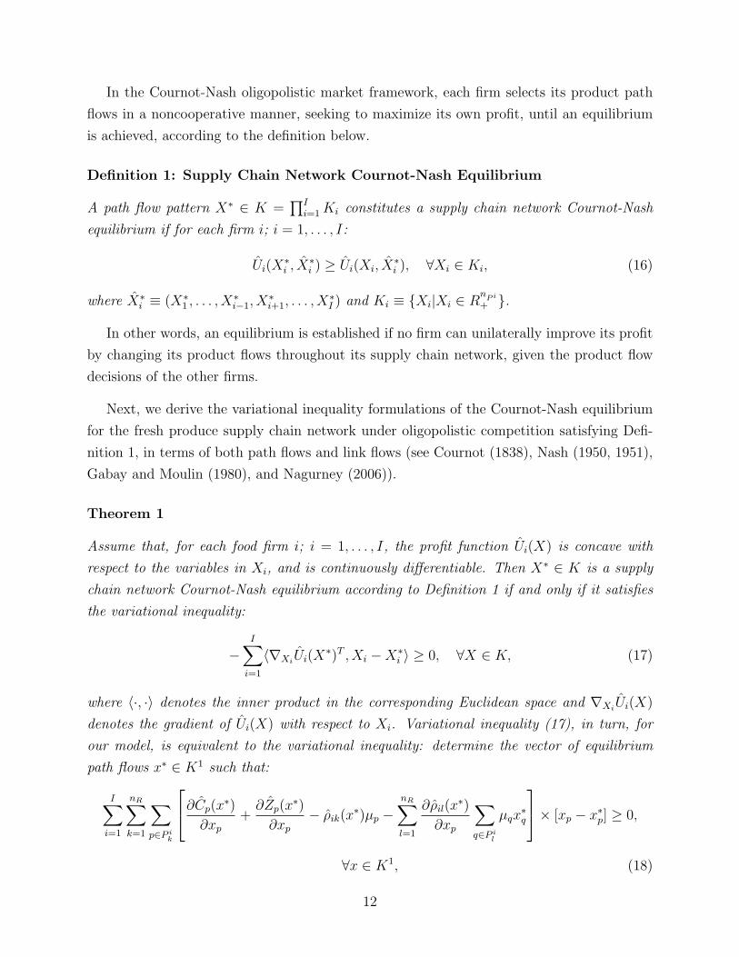
In the Cournot-Nash oligopolistic market framework, each firm selects its product path
flows in a noncooperative manner, seeking to maximize its own profit, until an equilibrium
is achieved, according to the definition below.
Definition 1: Supply Chain Network Cournot-Nash Equilibrium
A path flow pattern X∗ ∈ K =∏I
i=1 Ki constitutes a supply chain network Cournot-Nash
equilibrium if for each firm i; i = 1, . . . , I:
Ui(X∗i , X∗
i ) ≥ Ui(Xi, X∗i ), ∀Xi ∈ Ki, (16)
where X∗i ≡ (X∗
1 , . . . , X∗i−1, X
∗i+1, . . . , X
∗I ) and Ki ≡ {Xi|Xi ∈ R
nPi
+ }.
In other words, an equilibrium is established if no firm can unilaterally improve its profit
by changing its product flows throughout its supply chain network, given the product flow
decisions of the other firms.
Next, we derive the variational inequality formulations of the Cournot-Nash equilibrium
for the fresh produce supply chain network under oligopolistic competition satisfying Defi-
nition 1, in terms of both path flows and link flows (see Cournot (1838), Nash (1950, 1951),
Gabay and Moulin (1980), and Nagurney (2006)).
Theorem 1
Assume that, for each food firm i; i = 1, . . . , I, the profit function Ui(X) is concave with
respect to the variables in Xi, and is continuously differentiable. Then X∗ ∈ K is a supply
chain network Cournot-Nash equilibrium according to Definition 1 if and only if it satisfies
the variational inequality:
−I∑
i=1
〈∇XiUi(X
∗)T , Xi −X∗i 〉 ≥ 0, ∀X ∈ K, (17)
where 〈·, ·〉 denotes the inner product in the corresponding Euclidean space and ∇XiUi(X)
denotes the gradient of Ui(X) with respect to Xi. Variational inequality (17), in turn, for
our model, is equivalent to the variational inequality: determine the vector of equilibrium
path flows x∗ ∈ K1 such that:
I∑i=1
nR∑k=1
∑p∈P i
k
∂Cp(x∗)
∂xp
+∂Zp(x
∗)
∂xp
− ρik(x∗)µp −
nR∑l=1
∂ρil(x∗)
∂xp
∑q∈P i
l
µqx∗q
× [xp − x∗p] ≥ 0,
∀x ∈ K1, (18)
12
where K1 ≡ {x|x ∈ RnP+ }, and for each path p; p ∈ P i
k; i = 1, . . . , I; k = 1, . . . , nR,
∂Cp(x)
∂xp
≡∑a∈Li
∑b∈Li
∂cb(f)
∂fa
αap,∂Zp(x)
∂xp
≡∑a∈Li
∂za(fa)
∂fa
αap, and∂ρil(x)
∂xp
≡ ∂ρil(d)
∂dik
µp. (19)
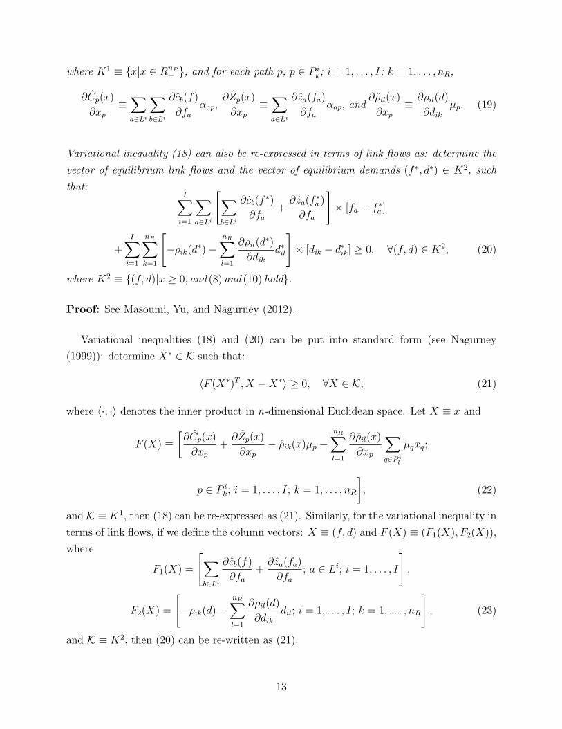
Variational inequality (18) can also be re-expressed in terms of link flows as: determine the
vector of equilibrium link flows and the vector of equilibrium demands (f ∗, d∗) ∈ K2, such
that:I∑
i=1
∑a∈Li
[∑b∈Li
∂cb(f∗)
∂fa
+∂za(f
∗a )
∂fa
]× [fa − f ∗a ]
+I∑
i=1
nR∑k=1
[−ρik(d
∗)−nR∑l=1
∂ρil(d∗)
∂dik
d∗il
]× [dik − d∗ik] ≥ 0, ∀(f, d) ∈ K2, (20)
where K2 ≡ {(f, d)|x ≥ 0, and (8) and (10) hold}.
Proof: See Masoumi, Yu, and Nagurney (2012).
Variational inequalities (18) and (20) can be put into standard form (see Nagurney
(1999)): determine X∗ ∈ K such that:
〈F (X∗)T , X −X∗〉 ≥ 0, ∀X ∈ K, (21)
where 〈·, ·〉 denotes the inner product in n-dimensional Euclidean space. Let X ≡ x and
F (X) ≡[∂Cp(x)
∂xp
+∂Zp(x)
∂xp
− ρik(x)µp −nR∑l=1
∂ρil(x)
∂xp
∑q∈P i
l
µqxq;
p ∈ P ik; i = 1, . . . , I; k = 1, . . . , nR
], (22)
and K ≡ K1, then (18) can be re-expressed as (21). Similarly, for the variational inequality in
terms of link flows, if we define the column vectors: X ≡ (f, d) and F (X) ≡ (F1(X), F2(X)),
where
F1(X) =
[∑b∈Li
∂cb(f)
∂fa
+∂za(fa)
∂fa
; a ∈ Li; i = 1, . . . , I
],
F2(X) =
[−ρik(d)−
nR∑l=1
∂ρil(d)
∂dik
dil; i = 1, . . . , I; k = 1, . . . , nR
], (23)
and K ≡ K2, then (20) can be re-written as (21).
13
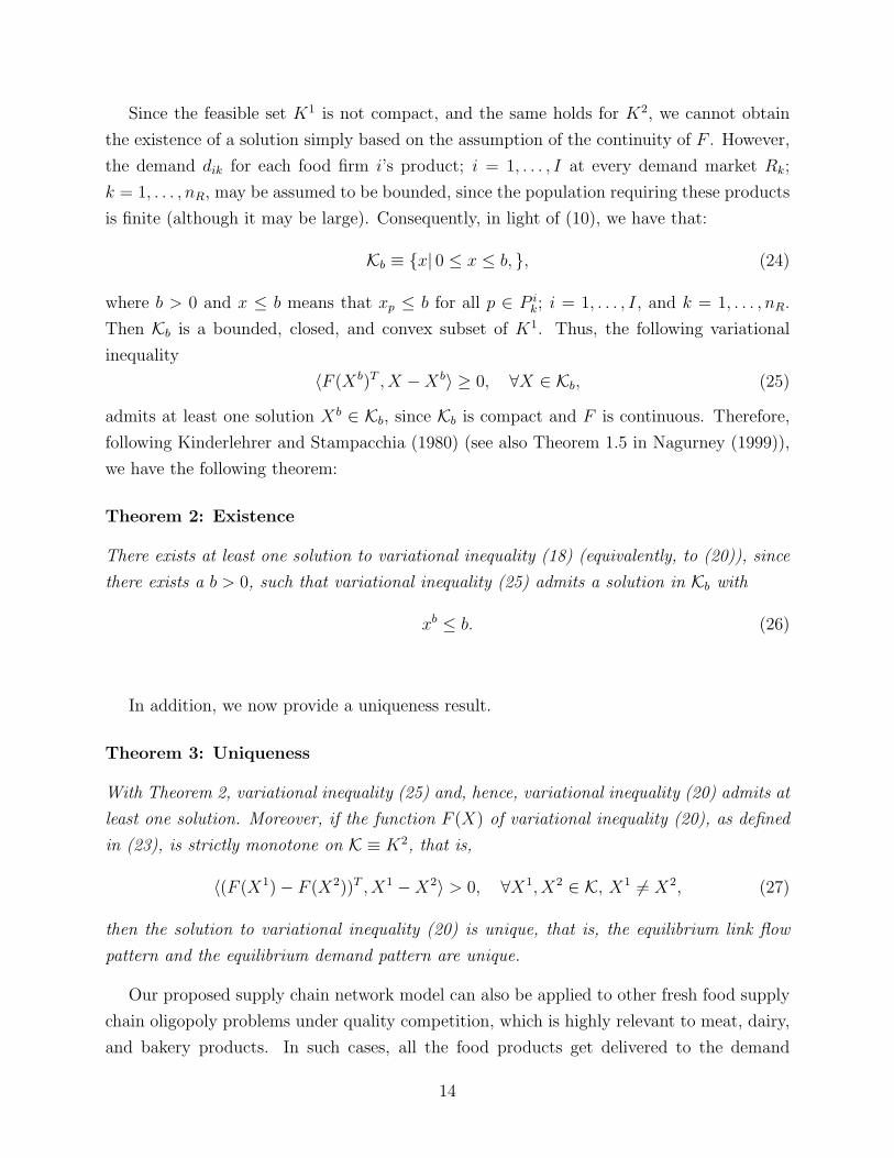
Since the feasible set K1 is not compact, and the same holds for K2, we cannot obtain
the existence of a solution simply based on the assumption of the continuity of F . However,
the demand dik for each food firm i’s product; i = 1, . . . , I at every demand market Rk;
k = 1, . . . , nR, may be assumed to be bounded, since the population requiring these products
is finite (although it may be large). Consequently, in light of (10), we have that:
Kb ≡ {x| 0 ≤ x ≤ b, }, (24)
where b > 0 and x ≤ b means that xp ≤ b for all p ∈ P ik; i = 1, . . . , I, and k = 1, . . . , nR.
Then Kb is a bounded, closed, and convex subset of K1. Thus, the following variational
inequality
〈F (Xb)T , X −Xb〉 ≥ 0, ∀X ∈ Kb, (25)
admits at least one solution Xb ∈ Kb, since Kb is compact and F is continuous. Therefore,
following Kinderlehrer and Stampacchia (1980) (see also Theorem 1.5 in Nagurney (1999)),
we have the following theorem:
Theorem 2: Existence
There exists at least one solution to variational inequality (18) (equivalently, to (20)), since
there exists a b > 0, such that variational inequality (25) admits a solution in Kb with
xb ≤ b. (26)
In addition, we now provide a uniqueness result.
Theorem 3: Uniqueness
With Theorem 2, variational inequality (25) and, hence, variational inequality (20) admits at
least one solution. Moreover, if the function F (X) of variational inequality (20), as defined
in (23), is strictly monotone on K ≡ K2, that is,
〈(F (X1)− F (X2))T , X1 −X2〉 > 0, ∀X1, X2 ∈ K, X1 6= X2, (27)
then the solution to variational inequality (20) is unique, that is, the equilibrium link flow
pattern and the equilibrium demand pattern are unique.
Our proposed supply chain network model can also be applied to other fresh food supply
chain oligopoly problems under quality competition, which is highly relevant to meat, dairy,
and bakery products. In such cases, all the food products get delivered to the demand
14
markets eventually, with distinct levels of quality degradation. Thus, the arc multiplier for
a post-production link, αa, captures the corresponding food quality degradation associated
with that link, instead of the number of the spoiled products. We refer to Labuza (1982)
and Man and Jones (1994) for thorough discussions about food quality deterioration.
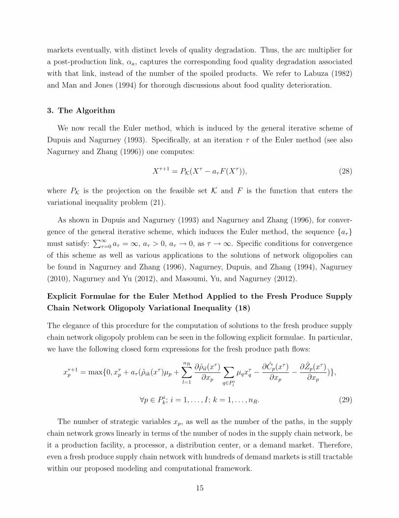
3. The Algorithm
We now recall the Euler method, which is induced by the general iterative scheme of
Dupuis and Nagurney (1993). Specifically, at an iteration τ of the Euler method (see also
Nagurney and Zhang (1996)) one computes:
Xτ+1 = PK(Xτ − aτF (Xτ )), (28)
where PK is the projection on the feasible set K and F is the function that enters the
variational inequality problem (21).
As shown in Dupuis and Nagurney (1993) and Nagurney and Zhang (1996), for conver-
gence of the general iterative scheme, which induces the Euler method, the sequence {aτ}must satisfy:
∑∞τ=0 aτ = ∞, aτ > 0, aτ → 0, as τ →∞. Specific conditions for convergence
of this scheme as well as various applications to the solutions of network oligopolies can
be found in Nagurney and Zhang (1996), Nagurney, Dupuis, and Zhang (1994), Nagurney
(2010), Nagurney and Yu (2012), and Masoumi, Yu, and Nagurney (2012).
Explicit Formulae for the Euler Method Applied to the Fresh Produce Supply
Chain Network Oligopoly Variational Inequality (18)
The elegance of this procedure for the computation of solutions to the fresh produce supply
chain network oligopoly problem can be seen in the following explicit formulae. In particular,
we have the following closed form expressions for the fresh produce path flows:
xτ+1p = max{0, xτ
p + aτ (ρik(xτ )µp +
nR∑l=1
∂ρil(xτ )
∂xp
∑q∈P i
l
µqxτq −
∂Cp(xτ )
∂xp
− ∂Zp(xτ )
∂xp
)},
∀p ∈ P ik; i = 1, . . . , I; k = 1, . . . , nR. (29)
The number of strategic variables xp, as well as the number of the paths, in the supply
chain network grows linearly in terms of the number of nodes in the supply chain network, be
it a production facility, a processor, a distribution center, or a demand market. Therefore,
even a fresh produce supply chain network with hundreds of demand markets is still tractable
within our proposed modeling and computational framework.
15
In the next Section, we solve fresh produce supply chain network oligopoly problems using
the above algorithmic scheme.
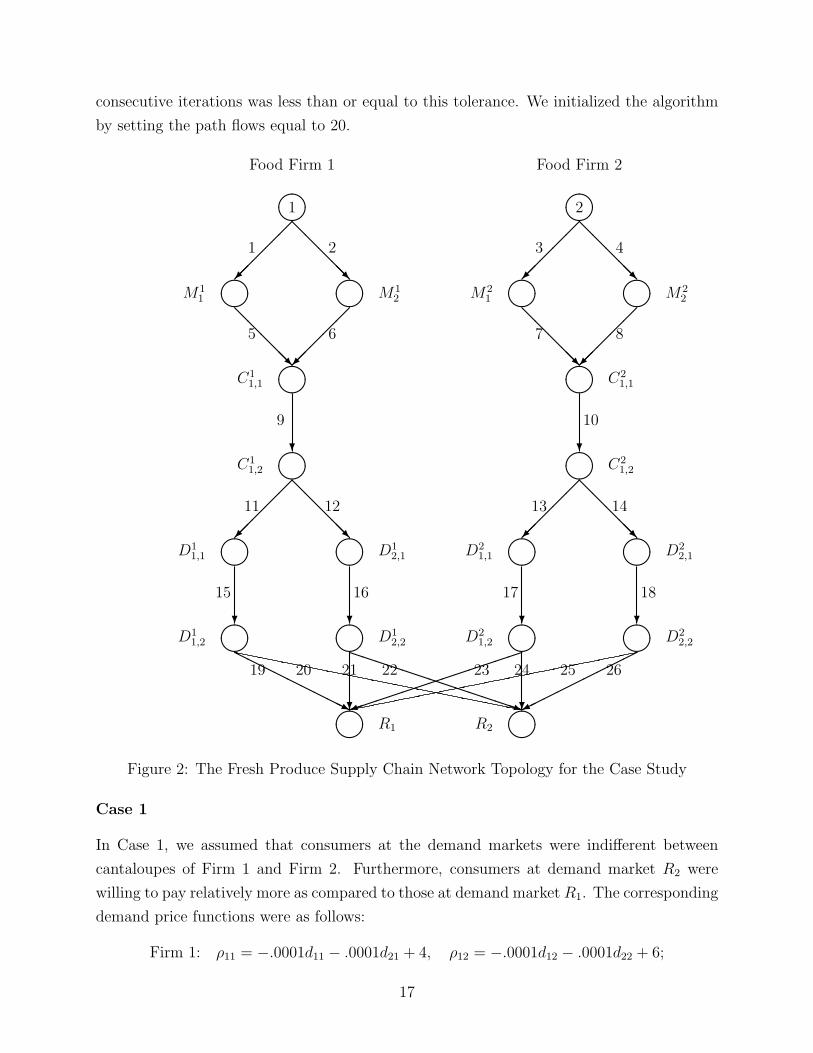
4. Case Study
In this Section, we focus on the cantaloupe market in the United States. Most of can-
taloupes consumed in the United States are originally produced in California, Mexico, and
in some countries in Central America. In our case study, there are two firms, Firm 1 and
Firm 2, which may represent, for example, one food firm in California and one food firm
in Central America, respectively. Each firm has two production sites, one processor, two
distribution centers, and serves two geographically separated demand markets, as depicted
in Figure 2. The production sites and the processor of Firm 1 are located in California,
whereas the production sites and the processor of Firm 2 are located in Central America,
with lower operational costs. However, all the distribution centers are located in the United
States as are the demand markets. The distribution centers D11 and D2
1 are located closer to
their respective production sites than the distribution centers D12 and D2
2 are. The demand
market R1 is located closer to the distribution centers D11 and D2
1, whereas the demand mar-
ket R2 is located closer to the distribution centers D12 and D2
2, that is, the demand market
R1 is located closer to the production sites.
Typically, cantaloupes can be stored for 12–15 days at 2.2◦ to 5◦C (36◦ to 41◦F) (Suslow,
Cantwell, and Mitchell (1997)). It has been noticed that the decay of cantaloupes may
result from such post-production disease as Rhizopus, Fusarium, Geotrichum, etc., depending
on the season, the region, and the handling technologies utilized between production and
consumption (see Suslow, Cantwell, and Mitchell (1997) and Sommer, Fortlage, and Edwards
(2002)). As discussed in Section 2, we captured the food deterioration through the arc
multipliers. The values of the decay rates and the time durations, although hypothetical,
were selected so as to reflect the different technologies associated with the various supply
chain activities. The values of the arc multipliers were, in turn, calculated using equation
(2), which captured the percentage of the spoiled fresh food products at the post-production
supply chain stages (see, e.g., Gustavsson et a l. (2011)). For instance, Firm 1 utilizes more
effective cleaning and sanitizing equipment for its processing activities of the cantaloupes,
which results in relatively higher operational costs, but lower decay rates associated with
the successive supply chain activities.
We implemented the Euler method (cf. (29)) for the solution of variational inequality
(18), using Matlab. We set the sequence aτ = .1(1, 12, 1
2, · · · ), and the convergence tolerance
was 10−6. In other words, the absolute value of the difference between each path flow in two
16
consecutive iterations was less than or equal to this tolerance. We initialized the algorithm
by setting the path flows equal to 20.
����R1 R2 ����
HHHHHHHHHj
PPPPPPPPPPPPPPq?
��������������) ?
����������
19 20 21 22 23 24 25 26
D11,2 ���� ����
D12,2 D2
1,2 ���� ����D2
2,2
? ? ? ?
15 16 17 18
D11,1 ���� ����
D12,1 D2
1,1 ���� ����D2
2,1
��
���
@@
@@@R
��
���
@@
@@@R
11 12 13 14
C11,2 ����
C21,2����? ?
9 10
C11,1 ����
C21,1����
@@
@@@R
��
���
@@
@@@R
��
���
5 6 7 8
M11 ���� ����
M12 M2
1 ���� ����M2
2
��
���
@@
@@@R
��
���
@@
@@@R
1 2 3 4
����1 ����
2
Food Firm 1 Food Firm 2
Figure 2: The Fresh Produce Supply Chain Network Topology for the Case Study
Case 1
In Case 1, we assumed that consumers at the demand markets were indifferent between
cantaloupes of Firm 1 and Firm 2. Furthermore, consumers at demand market R2 were
willing to pay relatively more as compared to those at demand market R1. The corresponding
demand price functions were as follows:
Firm 1: ρ11 = −.0001d11 − .0001d21 + 4, ρ12 = −.0001d12 − .0001d22 + 6;
17
Firm 2: ρ21 = −.0001d21 − .0001d11 + 4, ρ22 = −.0001d22 − .0001d12 + 6.
The arc multipliers, the total operational cost functions, and the total discarding cost
functions are reported in Table 1, as well as the decay rates (/day) and the time durations
(days) associated with all the links. These cost functions have been constructed based on
the data of the average costs available on the web (see, e.g., Meister (2004a, 2004b)).
Table 1 also provides the computed equilibrium product flows on all the links in Figure
2. The computed equilibrium demands for cantaloupes were:
d∗11 = 7.86, d∗12 = 123.62, d∗21 = 27.19, and d∗22 = 139.38.
The incurred equilibrium prices at each demand market were as follows:
ρ11 = 4.00, ρ12 = 5.97, ρ21 = 4.00, and ρ22 = 5.97.
Furthermore, the profits of two firms were:
U1 = 370.46, and U2 = 454.72.
Since consumers do not differentiate the cantaloupes produced by these two firms, the
prices of these two firms’ cantaloupes at each demand market are identical. Due to the
difference in consumers’ willingness to pay, the price at demand market R1 is relatively
lower than the price at demand market R2. Consequently, the distribution links: 21 and 25,
connecting Firm 1 and Firm 2 to demand market R1, respectively, have zero product flows.
In other words, there is no shipment from distribution centers D12 and D2
2 to demand market
R1. In addition, the volume of product flows on distribution link 22 (or link 26) is higher
than that of distribution link 20 (or link 24), which indicates that it is more cost-effective to
provide fresh fruits from the nearby distribution centers. As a result of its lower operational
costs, Firm 2 dominates both of these two demand markets, leading to a substantially higher
profit.
Case 2
The Centers for Disease Control (CDC) has reported 23 cantaloupe-associated outbreaks
between 1984 and 2002, which resulted in 1, 434 people falling ill, 42 hospitalizations, and 2
deaths (Bowen et al. (2006)). In Case 2, we considered the scenario that the CDC reported
a multi-state cantaloupe-associated outbreak. Due to food safety and health concerns, the
regular consumers of cantaloupes switched to other fresh fruits. The demand price functions
were no longer as in Case 1 and were given by:
Firm 1: ρ11 = −.001d11 − .001d21 + .5, ρ12 = −.001d12 − .001d22 + .5;
18

Table 1: Arc Multipliers, Total Operational Cost and Total Discarding Cost Functions, andEquilibrium Link Flow Solution for Case 1
Link a λa ta αa ca(f) za(fa) f ∗a1 – – 1.00 .005f 2
1 + .03f1 0.00 76.322 – – 1.00 .006f 2
2 + .02f2 0.00 75.733 – – 1.00 .001f 2
3 + .02f3 0.00 103.744 – – 1.00 .001f 2
4 + .02f4 0.00 105.625 .150 0.20 .970 .003f 2
5 + .01f5 0.00 76.326 .150 0.25 .963 .002f 2
6 + .02f6 0.00 75.737 .150 0.30 .956 .001f 2
7 + .02f7 0.00 103.748 .150 0.30 .956 .001f 2
8 + .01f8 0.00 105.629 .040 0.50 .980 .002f 2
9 + .05f9 .001f 29 + 0.02f9 147.01
10 .060 0.50 .970 .001f 210 + .02f10 .001f 2
10 + 0.02f10 200.1411 .015 1.50 .978 .005f 2
11 + .01f11 0.00 65.9812 .015 3.00 .956 .01f 2
12 + .01f12 0.00 78.1213 .025 2.00 .951 .005f 2
13 + .02f13 0.00 96.4714 .025 4.00 .905 .01f 2
14 + .01f14 0.00 97.7615 .010 3.00 .970 .004f 2
15 + .01f15 .001f 215 + 0.02f15 64.51
16 .010 3.00 .970 .004f 216 + .01f16 .001f 2
16 + 0.02f16 74.6817 .015 3.00 .956 .004f 2
17 + .01f17 .001f 217 + 0.02f17 91.77
18 .015 3.00 .956 .004f 218 + .01f18 .001f 2
18 + 0.02f18 88.4519 .015 1.00 .985 .005f 2
19 + .01f19 .001f 219 + 0.02f19 7.98
20 .015 3.00 .956 .015f 220 + .1f20 .001f 2
20 + 0.02f20 54.6221 .015 3.00 .956 .015f 2
21 + .1f21 .001f 221 + 0.02f21 0.00
22 .015 1.00 .985 .005f 222 + .01f22 .001f 2
22 + 0.02f22 72.4823 .020 1.00 .980 .005f 2
23 + .01f23 .001f 223 + 0.02f23 27.74
24 .020 3.00 .942 .015f 224 + .1f24 .001f 2
24 + 0.02f24 59.9925 .020 3.00 .942 .015f 2
25 + .1f25 .001f 225 + 0.02f25 0.00
26 .020 1.00 .980 .005f 226 + .01f26 .001f 2
26 + 0.02f26 84.56
19
Firm 2: ρ21 = −.001d21 − .001d11 + .5, ρ22 = −.001d22 − .001d12 + .5.
The longer time durations associated with shipment links 13 and 14 in Table 2, represent
the prolonged transportation from Firm 2’s processor to its distribution centers in the United
States, because of more imported food inspections by the U.S. Food and Drug Administration
(FDA). Therefore, the values of arc multipliers associated with links 13 and 14 in Table 2
are lower than those in Table 1, which implies more perished cantaloupes generated at this
stage. The other arc multipliers, the total operational and the total discarding cost functions
are the same as in Case 1, as shown in Table 2. The new computed equilibrium link flows
are also reported in Table 2.
The computed equilibrium demands for cantaloupes were:
d∗11 = 4.51, d∗12 = 3.24, d∗21 = 5.96, and d∗22 = 4.21.
The incurred equilibrium prices at each demand market were as follows:
ρ11 = 0.49, ρ12 = 0.49, ρ21 = 0.49, and ρ22 = 0.49.
Furthermore, the profits of two firms were:
U1 = 1.16, and U2 = 1.63.
The demand for cantaloupes is battered by the cantaloupe-associated outbreak, with
significant decreases in demand prices at demand markets R1 and R2. Both Firm 1 and Firm
2, in turn, experience dramatic declines in their profits. In addition, additional distribution
links: 20, 21, 24, and 25, have zero product flows (as compared to Case 1), since the extremely
low demand price cannot cover the costs associated with long-distance distribution.
Case 3
Given the severe shrinkage in the demand for cantaloupes, Firm 1 has realized the impor-
tance of regaining consumers’ confidence in its own product after the cantaloupe-associated
outbreak. Thus, Firm 1 had its label of cantaloupes redesigned in order to incorporate the
guarantee of food safety, with additional expenditures associated with its processing activi-
ties. The demand price functions corresponding to the two demand markets for cantaloupes
from these two firms were given by:
Firm 1: ρ11 = −.001d11 − .0005d21 + 2.5, ρ12 = −.0003d12 − .0002d22 + 3;
Firm 2: ρ21 = −.001d21 − .001d11 + .5, ρ22 = −.001d22 − .001d12 + .5.
20

Table 2: Arc Multipliers, Total Operational Cost and Total Discarding Cost Functions, andEquilibrium Link Flow Solution for Case 2
Link a λa ta αa ca(f) za(fa) f ∗a1 – – 1.00 .005f 2
1 + .03f1 0.00 4.432 – – 1.00 .006f 2
2 + .02f2 0.00 4.403 – – 1.00 .001f 2
3 + .02f3 0.00 5.944 – – 1.00 .001f 2
4 + .02f4 0.00 6.945 .150 0.20 .970 .003f 2
5 + .01f5 0.00 4.436 .150 0.25 .963 .002f 2
6 + .02f6 0.00 4.407 .150 0.30 .956 .001f 2
7 + .02f7 0.00 5.948 .150 0.30 .956 .001f 2
8 + .01f8 0.00 6.949 .040 0.50 .980 .002f 2
9 + .05f9 .001f 29 + 0.02f9 8.53
10 .060 0.50 .970 .001f 210 + .02f10 .001f 2
10 + 0.02f10 12.3111 .015 1.50 .978 .005f 2
11 + .01f11 0.00 4.8212 .015 3.00 .956 .01f 2
12 + .01f12 0.00 3.5413 .025 3.00 .928 .005f 2
13 + .02f13 0.00 6.8614 .025 5.00 .882 .01f 2
14 + .01f14 0.00 5.0915 .010 3.00 .970 .004f 2
15 + .01f15 .001f 215 + 0.02f15 4.72
16 .010 3.00 .970 .004f 216 + .01f16 .001f 2
16 + 0.02f16 3.3817 .015 3.00 .956 .004f 2
17 + .01f17 .001f 217 + 0.02f17 6.36
18 .015 3.00 .956 .004f 218 + .01f18 .001f 2
18 + 0.02f18 4.4919 .015 1.00 .985 .005f 2
19 + .01f19 .001f 219 + 0.02f19 4.58
20 .015 3.00 .956 .015f 220 + .1f20 .001f 2
20 + 0.02f20 0.0021 .015 3.00 .956 .015f 2
21 + .1f21 .001f 221 + 0.02f21 0.00
22 .015 1.00 .985 .005f 222 + .01f22 .001f 2
22 + 0.02f22 3.2823 .020 1.00 .980 .005f 2
23 + .01f23 .001f 223 + 0.02f23 6.08
24 .020 3.00 .942 .015f 224 + .1f24 .001f 2
24 + 0.02f24 0.0025 .020 3.00 .942 .015f 2
25 + .1f25 .001f 225 + 0.02f25 0.00
26 .020 1.00 .980 .005f 226 + .01f26 .001f 2
26 + 0.02f26 4.29
21
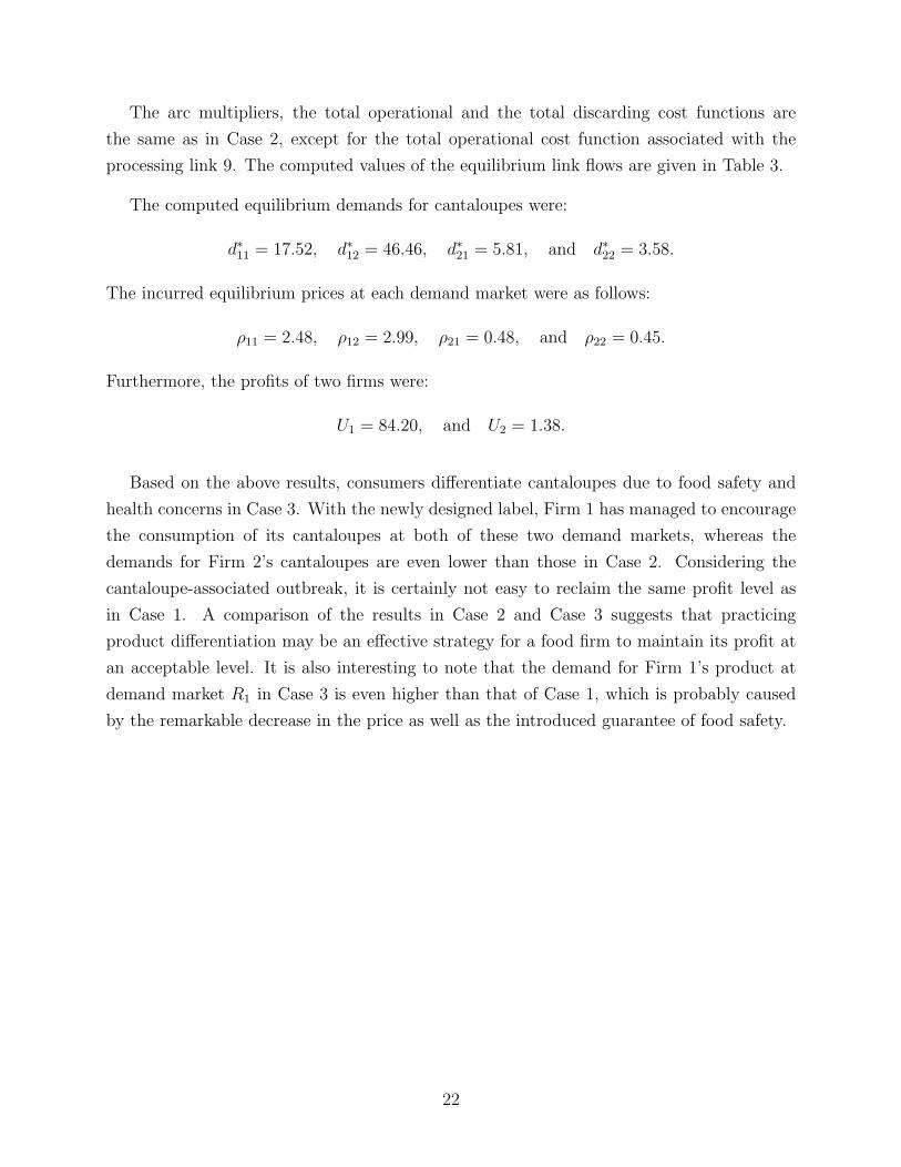
The arc multipliers, the total operational and the total discarding cost functions are
the same as in Case 2, except for the total operational cost function associated with the
processing link 9. The computed values of the equilibrium link flows are given in Table 3.
The computed equilibrium demands for cantaloupes were:
d∗11 = 17.52, d∗12 = 46.46, d∗21 = 5.81, and d∗22 = 3.58.
The incurred equilibrium prices at each demand market were as follows:
ρ11 = 2.48, ρ12 = 2.99, ρ21 = 0.48, and ρ22 = 0.45.
Furthermore, the profits of two firms were:
U1 = 84.20, and U2 = 1.38.
Based on the above results, consumers differentiate cantaloupes due to food safety and
health concerns in Case 3. With the newly designed label, Firm 1 has managed to encourage
the consumption of its cantaloupes at both of these two demand markets, whereas the
demands for Firm 2’s cantaloupes are even lower than those in Case 2. Considering the
cantaloupe-associated outbreak, it is certainly not easy to reclaim the same profit level as
in Case 1. A comparison of the results in Case 2 and Case 3 suggests that practicing
product differentiation may be an effective strategy for a food firm to maintain its profit at
an acceptable level. It is also interesting to note that the demand for Firm 1’s product at
demand market R1 in Case 3 is even higher than that of Case 1, which is probably caused
by the remarkable decrease in the price as well as the introduced guarantee of food safety.
22
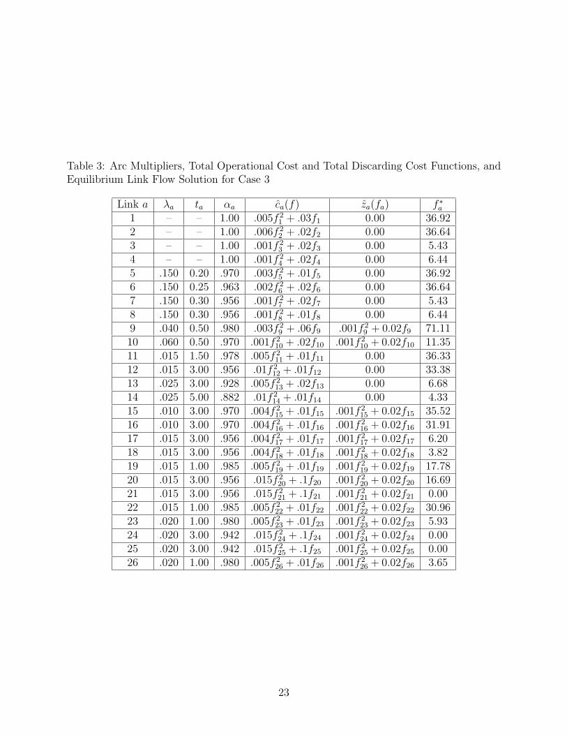
Table 3: Arc Multipliers, Total Operational Cost and Total Discarding Cost Functions, andEquilibrium Link Flow Solution for Case 3
Link a λa ta αa ca(f) za(fa) f ∗a1 – – 1.00 .005f 2
1 + .03f1 0.00 36.922 – – 1.00 .006f 2
2 + .02f2 0.00 36.643 – – 1.00 .001f 2
3 + .02f3 0.00 5.434 – – 1.00 .001f 2
4 + .02f4 0.00 6.445 .150 0.20 .970 .003f 2
5 + .01f5 0.00 36.926 .150 0.25 .963 .002f 2
6 + .02f6 0.00 36.647 .150 0.30 .956 .001f 2
7 + .02f7 0.00 5.438 .150 0.30 .956 .001f 2
8 + .01f8 0.00 6.449 .040 0.50 .980 .003f 2
9 + .06f9 .001f 29 + 0.02f9 71.11
10 .060 0.50 .970 .001f 210 + .02f10 .001f 2
10 + 0.02f10 11.3511 .015 1.50 .978 .005f 2
11 + .01f11 0.00 36.3312 .015 3.00 .956 .01f 2
12 + .01f12 0.00 33.3813 .025 3.00 .928 .005f 2
13 + .02f13 0.00 6.6814 .025 5.00 .882 .01f 2
14 + .01f14 0.00 4.3315 .010 3.00 .970 .004f 2
15 + .01f15 .001f 215 + 0.02f15 35.52
16 .010 3.00 .970 .004f 216 + .01f16 .001f 2
16 + 0.02f16 31.9117 .015 3.00 .956 .004f 2
17 + .01f17 .001f 217 + 0.02f17 6.20
18 .015 3.00 .956 .004f 218 + .01f18 .001f 2
18 + 0.02f18 3.8219 .015 1.00 .985 .005f 2
19 + .01f19 .001f 219 + 0.02f19 17.78
20 .015 3.00 .956 .015f 220 + .1f20 .001f 2
20 + 0.02f20 16.6921 .015 3.00 .956 .015f 2
21 + .1f21 .001f 221 + 0.02f21 0.00
22 .015 1.00 .985 .005f 222 + .01f22 .001f 2
22 + 0.02f22 30.9623 .020 1.00 .980 .005f 2
23 + .01f23 .001f 223 + 0.02f23 5.93
24 .020 3.00 .942 .015f 224 + .1f24 .001f 2
24 + 0.02f24 0.0025 .020 3.00 .942 .015f 2
25 + .1f25 .001f 225 + 0.02f25 0.00
26 .020 1.00 .980 .005f 226 + .01f26 .001f 2
26 + 0.02f26 3.65
23
5. Summary and Conclusions
This paper focused on food deterioration between production and consumption locations,
which poses unique challenges to food supply chain management. In particular, we developed
a network-based food supply chain model under oligopolistic competition and perishability,
with a concentration in fresh produce, such as vegetables and fruits. Each food firm is
involved in such supply chain activities as the production, processing, storage, distribution,
and even the disposal of the food products, and seeks to determine its optimal product flows
throughout its supply chain, in order to maximize its own profit.
We captured the food exponential time decay in number of units through the introduction
of arc multipliers, which depend on the time duration and environmental conditions associ-
ated with each post-production supply chain activity. We also incorporated the discarding
costs associated with the disposal of the spoiled food products at the processing, storage,
and distribution stages. Moreover, the competitive model allows consumers to differentiate
food products at the demand markets due to product freshness and food safety concerns.
In addition, the flexibility of the supply chain network topology allows decision-makers to
evaluate alternative technologies involved in various supply chain activities.
We derived the variational inequality formulations of the food supply chain network
Cournot-Nash equilibrium conditions, and studied the qualitative properties of the equi-
librium pattern. We also adopted an algorithm which yields subproblems at each iteration
with nice features for computation. We then illustrated the proposed model as well as the
algorithm by presenting several numerical cases, which focused on the cantaloupe market in
the United States. The results of the case study suggested that product differentiation may
be an effective strategy for a firm to keep itself financially resilient, especially in times of
outbreaks of foodborne diseases.
We emphasized that our model can be applied – albeit after appropriate modifications –
to other perishable product supply chain problems under oligopolistic competition, and even
with quality competition. Possible extensions could include the incorporation of supply side
as well as demand side variability, such as demand price volatility and delivery reliability.
In addition, the development of food supply chain network design models with capacities
associated with various supply chain activities being strategic variables (see Nagurney (2010))
is an interesting future research direction.
Acknowledgments
The authors acknowledge the helpful comments and suggestions of two anonymous reviewers
24
on an earlier version of this paper.
This research was supported, in part, by the John F. Smith Memorial Foundation at the
Isenberg School of Management at the University of Massachusetts Amherst. This support
is gratefully appreciated.
The second author also acknowledges the support from the School of Business, Economics
and Law at the University of Gothenburg in Gothenburg, Sweden, where she is a Visiting
Professor of Operations Management for 2012-2013.
References
Ahumada, O., Villalobos, J. R., 2009. Application of planning models in the agri-food supply
chain: A review. European Journal of Operational Research 195, 1-20.
Ahumada, O., Villalobos, J. R., 2011. A tactical model for planning the production and
distribution of fresh produce. Annals of Operations Research 190, 339-358.
Aiello, G., La Scalia, G., Micale, R., 2012. Simulation analysis of cold chain performance
based on time-temperature data. Production Planning & Control 23(6), 468-476.
Akkerman, R., Farahani, P., Grunow, M., 2010. Quality, safety and sustainability in food
distribution: A review of quantitative operations management approaches and challenges.
OR Spectrum 32, 863-904.
Aramyan, C., Ondersteijn, O., van Kooten, O., Lansink, A. O., 2006. Performance indi-
cators in agri-food production chains. In Quantifying the Agri-Food Supply Chain,
Ondersteijn, C. J. M., Wijnands, J. H. M., Huirne, R. B. M., and Van Kooten, O. (Editors),
Springer, Dordrecht, The Netherlands, pp 49-66.
Blackburn, J., Scudder, G., 2009. Supply chain strategies for perishable products: The case
of fresh produce. Production and Operations Management 18(2), 129-137.
Boehlje, M., 1999. Structural changes in the agricultural industries: How do we measure,
analyze and understand them? American Journal of Agricultural Economics 81(5), 1028-
1041.
Bowen, A., Fry, A., Richards, G., Beuchat, L., 2006. Infections associated with cantaloupe
consumption: A public health concerns. Epidemiology and Infection 134, 675-685.
Cook, R. L., 2002. The U.S. fresh produce industry: An industry in transition. In Posthar-
25
vest Technology of Horticultural Crops, third edition, Kader, A. A. (Editor), Univer-
sity of California Agriculture & Natural Resources, Publication 3311, Oakland, CA, USA,
pp 5-30.
Cournot, A. A., 1838. Researches into the Mathematical Principles of the Theory
of Wealth, English translation, MacMillan, London, England, 1897.
Dupuis, P., Nagurney, A., 1993. Dynamical systems and variational inequalities. Annals of
Operations Research 44, 9-42.
Fu, B., Labuza, T. P., 1993. Shelf-life prediction: Theory and application. Food Control
4(3), 125-133.
Gabay, D., Moulin, H., 1980. On the uniqueness and stability of Nash equilibria in noncoop-
erative games. In: Applied Stochastic Control of Econometrics and Management
Science, Bensoussan, A., Kleindorfer, P., Tapiero, C. S. (Editors), North-Holland, Amster-
dam, The Netherlands, pp. 271-294.
Ghare, P., Schrader, G., 1963. A model for an exponentially decaying inventory. Journal of
Industrial Engineering 14, 238-243.
Glen, J. J., 1987. Mathematical models in farm planning: A survey. Operations Research
35(5), 641-666.
Gustavsson, J., Cederberg, C., Sonesson, U., van Otterdijk, R., Meybeck, A., 2011. Global
food losses and food waste. The Food and Agriculture Organization of the United Nations,
Rome, Italy.
Karkkainen, M., 2003. Increasing efficiency in the supply chain for short shelf life goods
using RFID tagging. International Journal of Retail & Distribution Management 31(10),
529-536.
Kinderlehrer, D., Stampacchia, G., 1980. An Introduction to Variational Inequalities
and Their Applications. Academic Press, New York, USA.
Kopanos, G. M., Puigjaner, L., Georgiadis, M. C., 2012. Simultaneous production and
logistics operations planning in semicontinuous food industries. Omega 40, 634-650.
Labuza, T. P., 1982. Shelf-life Dating of Foods. Food & Nutrition Press, Westport, CT,
USA.
26
Liu, Z., Nagurney, A., 2012. Multiperiod competitive supply chain networks with inventory-
ing and a transportation network equilibrium reformulation. Optimization and Engineering,
in press.
Lowe, T. J., Preckel, P. V., 2004. Decision technologies for agribusiness problems: A brief
review of selected literature and a call for research. Manufacturing & Service Operations
Management 6(3), 201-208.
Lucas, M. T., Chhajed, D., 2004. Applications of location analysis in agriculture: A survey.
Journal of the Operational Research Society 55(6), 561-578.
Lusk, J. L., Hudson, D., 2004. Willingness-to-pay estimates and their relevance to agribusi-
ness decision making. Review of Agricultural Economics 26(2), 152-169.
Lutke Entrup, M., 2005. Advanced Planning in Fresh Food Industries: Integrating
Shelf Life into Production Planning, Physica-Verlag/Springer, Heidelberg, Germany.
Lutke Entrup, M., Gunther, H.-O., van Beek, P., Grunow, M., Seiler, T., 2005. Mixed-
integer linear programming approaches to shelf-life-integrated planning and scheduling in
yogurt production. International Journal of Production Research 43(23), 5071-5100.
Man, C. M. D., Jones, A. A.,1994. Shelf Life Evaluation of Foods. Blackie Academic &
Professional, Glasgow, UK.
Masoumi, A. H., Yu, M., Nagurney, A., 2012. A supply chain generalized network oligopoly
model for pharmaceuticals under brand differentiation and perishability. Transportation
Research E 48, 762-780.
Meister, H. S., 2004a. Sample cost to establish and produce cantaloupes (slant-bed, spring
planted). U.C. Cooperative Extension – Imperial County Vegetable Crops Guidelines, Au-
gust 2004.
Meister, H. S., 2004b. Sample cost to establish and produce cantaloupes (mid-bed trenched).
U.C. Cooperative Extension – Imperial County Vegetable Crops Guidelines, August 2004.
Monteiro, D. M. S., 2007. Theoretical and empirical analysis of the economics of traceabil-
ity adoption in food supply chains. Ph.D. Thesis, University of Massachusetts Amherst,
Amherst, MA, USA.
Nagurney, A., 1999. Network Economics: A Variational Inequality Approach, sec-
27
ond and revised edition. Kluwer Academic Publishers, Boston, MA, USA.
Nagurney, A., 2006. Supply Chain Network Economics: Dynamics of Prices, Flows
and Profits. Edward Elgar Publishing Inc., Cheltenham, UK.
Nagurney, A., 2010. Supply chain network design under profit maximization and oligopolistic
competition. Transportation Research E 46, 281-294.
Nagurney, A., Aronson, J., 1989. A general dynamic spatial price network equilibrium model
with gains and losses. Networks 19(7), 751-769.
Nagurney, A., Dupuis, P., Zhang, D., 1994. A dynamical systems approach for network
oligopolies and variational inequalities. Annals of Regional Science 28, 263-283.
Nagurney, A., Masoumi, A. H., 2012. Supply chain network design of a sustainable blood
banking system. In: Sustainable Supply Chains: Models, Methods and Public
Policy Implications, Boone, T., Jayaraman, V., and Ganeshan, R. (Editors), Springer,
London, England, pp 47-72.
Nagurney, A., Masoumi, A. H., Yu, M., 2012. Supply chain network operations management
of a blood banking system with cost and risk minimization. Computational Management
Science 9(2), 205-231.
Nagurney, A., Nagurney, L., 2012. Medical nuclear supply chain design: A tractable network
model and computational approach. International Journal of Production Economics, in
press.
Nagurney, A., Yu, M., 2012. Sustainable fashion supply chain management under oligopolis-
tic competition and brand differentiation. International Journal of Production Economics
135, 532-540.
Nagurney, A., Zhang, D., 1996. Projected Dynamical Systems and Variational In-
equalities with Applications. Kluwer Academic Publishers, Norwell, MA, USA.
Nahmias, S., 1982. Perishable inventory theory: A review. Operations Research 30(4),
680-708.
Nahmias, S., 2011. Perishable Inventory Systems, Springer, New York, USA.
Nash, J. F., 1950. Equilibrium points in n-person games. Proceedings of the National
Academy of Sciences, USA 36, 48-49.
28
Nash, J. F., 1951. Noncooperative games. Annals of Mathematics 54, 286-298.
Nga, M. T. T., 2010. Enhancing quality management of fresh fish supply chains through
improved logistics and ensured traceability. Ph.D. Thesis, University of Iceland, Reykjavik,
Iceland.
Plunkett Research, 2011. U.S. food industry overview. Available online at: http://www.plun
kettresearch.com/food%20beverage%20grocery%20market%20research/industry%20statistics.
Rong, A., Akkerman, R., Grunow, M., 2011. An optimization approach for managing fresh
food quality throughout the supply chain. International Journal of Production Economics
131(1), 421-429.
Silver, E. A., Pyke, D. F., Peterson, R., 1998. Inventory Management and Production
Planning and Scheduling, third edition. John Wiley & Sons, New York, USA.
Sloof, M., Tijskens, L. M. M., Wilkinson, E. C., 1996. Concepts for modelling the quality of
perishable products. Trends in Food Science & Technology 7(5), 165-171.
Smith, D., Sparks, L., 2004. Temperature controlled supply chains. In Food Supply Chain
Management, Bourlakis, M., and Weightman, P. (Editors), Blackwell Publishing, Oxford,
UK, pp 179-198.
Sommer, N. F., Fortlage, R. J., Edwards, D. C., 2002. Postharvest diseases of selected
commodities. In Postharvest Technology of Horticultural Crops, third edition, Kader,
A. A. (Editor), University of California Agriculture & Natural Resources, Publication 3311,
Oakland, CA, USA, pp 197-249.
Suslow, T. V., Cantwell, M., Mitchell, J., 1997. Cantaloupe: Recommendations for main-
taining postharvest quality. Department of Vegetable Crops, University of California, Davis,
CA, USA.
Thompson, J. F., 2002. Waste management and cull utilization. In Postharvest Technol-
ogy of Horticultural Crops, third edition, Kader, A. A. (Editor), University of California
Agriculture & Natural Resources, Publication 3311, Oakland, CA, USA, pp 81-84.
Tijskens, L. M. M., Polderdijk, J. J., 1996. A generic model for keeping quality of vegetable
produce during storage and distribution. Agricultural Systems 51(4), 431-452.
Trienekens, J., Zuurbier, P., 2008. Quality and safety standards in the food industry, devel-
29
opments and challenges. International Journal of Production Economics 113, 107-122.
United States Department of Agriculture (USDA), 2011. Fruits and vegetables (farm weight):
Per capita availability, 1970–2009. Available online at: http://www.ers.usda.gov/Data/Food
Consumption/spreadsheets/fruitveg.xls.
Van der Vorst, J. G. A. J., 2000. Effective food supply chains: Generating, modelling and
evaluating supply chain scenarios. Ph.D. thesis, Wageningen University, The Netherlands.
Van der Vorst, J. G. A. J., 2006. Performance measurement in agri-food supply-chain net-
works: An overview. In Quantifying the Agri-Food Supply Chain, Ondersteijn, C.
J. M., Wijnands, J. H. M., Huirne, R. B. M., and van Kooten, O. (Editors), Springer,
Dordrecht, The Netherlands, pp 15-26.
Van Zyl, G. J. J., 1964. Inventory control for perishable commodities. Ph.D. Thesis, Uni-
versity of North Carolina at Chapel Hill, Chapel Hill, NC, USA.
Widodo, K. H., Nagasawa, H., Morizawa, K., Ota, M., 2006. A periodical flowering-
harvesting model for delivering agricultural fresh products. European Journal of Operational
Research 170, 24-43.
Wilcock, A., Pun, M., Khanona, J., Aung, M., 2004. Consumer attitudes, knowledge and
behaviour: A review of food safety issues. Trends in Food Science & Technology 15(2), 56-66.
Zhang, G., Habenicht, W., Spieß, W. E. L., 2003. Improving the structure of deep frozen
and chilled food chain with tabu search procedure. Journal of Food Engineering 60, 67-79.
30