Competition between Blended Traditional and...

Competition between Blended Traditional and Virtual Sellers

Paper 241 T. Randolph Beard Gary Madden

July 2008

A research and education initiative at the MIT Sloan School of Management

For more information,

[email protected] or 617-253-7054 please visit our website at http://digital.mit.edu

or contact the Center directly at

Competition between Blended Traditional and Virtual Sellers*†

T. Randolph Beard

Department of Economics Auburn University Auburn, AL 36849

USA

Gary Madden Department of Economics

Curtin University of Technology Perth, WA 6845

Australia

8 June 2008

Abstract Competition in many electronic markets involves rivalry between ‘Bricks and Clicks’ firms, which operate both traditional and on-line vendors, and entrants who rely completely on Internet sales. In many cases, the goods being offered are identical-only the channels by which they are distributed differ. This structure is understood as reflecting temporal experimentation by firms operating in an environment of incomplete information about consumer preferences and costs. Both demand characteristics and production costs can be expected to differ between traditional and virtual distribution networks. Further, the blended channel seller faces the issue of cannibalization of demand upon virtual market entry. This article analyses post-entry performance of a unique sample of Australian virtual entrants who face incumbent blended channel competitors. The fate of these entrants depends not just on their abilities to discern relevant parameters of the underlying environment, but also on incumbent response to entry. The incumbents, in turn, can limit entrant penetration by their virtual operations, but such operations involve loss of sales in the Bricks and Mortar market segment. We seek to identify and characterize those features of product markets and cost conditions consistent with survival of virtual entrants as a long-run equilibrium phenomenon. JEL Classification: L86, D21, L1, O33 Keywords: E-Commerce, Technology adoption, Retail industries

*Comments welcome, [email protected]; [email protected]. † The MIT Center for Digital Business and the Columbia Institute for Tele-Information provided support during the time this paper was revised. Helpful comments were provided by participants in seminars at Columbia University and Curtin University of Technology. We are very grateful to Warren Kimble and Aaron Morey for excellent research assistance. The authors are responsible for all remaining errors.

1. Introduction The OECD considers Internet users, hosts and access price, and secure servers accurately reflect the state of Member Country e-commerce readiness. In particular, in 2004-05 Australian firms’ personal computer and Internet penetration levels are 89% and 77%, respectively (EIU, 2007). Furthermore, during 2005-06, 20.9% of Australian firms received orders on-line, while 37.3% placed Internet orders. This asymmetric activity is thought to reflect that placement of on-line orders only requires access to a computer with an Internet connection, whereas receiving orders necessitates an established Web presence with technical support (Australian Bureau of Statistics; ABS, 2006). Importantly, the ABS (2006) identifies that placement of orders via the Internet (or Web) increases with firms’ employment, viz., 33% for firms with 0-4 employees compared to 67% for firms with more than 200 employees placed on-line orders. The pattern for receiving orders on-line is similar, viz., 19% for firms with 0-4 employees and 28% for firms with more than 20 employees. Also, Internet revenue from on-line orders grew from $40 billion in 2004-05 to $57 billion in 2005-06. This 2005-06 Internet revenue is approximately 3% of goods and service, and total business revenue. Of the 21% of Australian firms that received Internet orders in 2005-06, 64% generated 5% or more of their income from Internet sales (OECD, 2006). This concentration of e-commerce is larger firms is rationalised as being caused by smaller firms having a lack of strategic awareness and technical knowledge, mistrust of technology, and high establishment costs (DBCDE, 2002; Dunt and Harper, 2002; OECD, 2004). Competition in many of these electronic markets involves rivalry between ‘Bricks and Clicks’ firms, which operate as both traditional and on-line vendors, and entrants that rely completely on Internet selling. Often the goods being offered for sale are identical, and only the channels by which they are distributed differ. This structure is suggestive of temporal experimentation by firms operating in an environment with incomplete information about consumer preferences and costs. Both demand characteristics and production costs can be expected to differ between traditional and virtual distribution networks. Further, blended channel sellers face an issue of demand cannibalization on virtual market entry. Additionally, while the above reports clearly indicate that small and large firms exhibit substantially different tendencies to embrace the new technology, adoption rates also differ by product category (ABS, 2006). These patterns suggest several related questions: How do virtual firms differ in their adoption patterns? In what type of environments is post on-line market entry performance by virtual and established firms likely to succeed? What can be said about the relationship between post-entry performance and the reasons for entry? Much of the empirical industrial organization literature on market turbulence (firm entry, exit and survival) concerns the analysis of firm population cohort data (Fotopoulos and Louri 2000, Mahmood 2000, Segarra and Callejón 2002, Disney et al. 2003). A unifying theme of this literature is the entry equation,

*j j j jE B eαπ γ= − +

2

where E is the number of firms entering market j , and is explained by *π the profits expected to occur in market j and costs that follow the entry decision B and e is a random error. Overviews of this literature by Geroski (1995) and Caves (1998) suggest that entry is relatively easy, but survival is not. The most palpable consequence of entry is exit. As most entry attempts ultimately fail, and as most entrants take five to ten years before they are able to compete on a par with incumbents, incumbents find costly attempts to deter entry unprofitable. Furthermore, the role entry plays in shaping industry structure is bound up with the proposition that entry is often a vehicle for introducing innovation, particularly in early phases of industry evolution (Geroski 1995: 436). At some point in new market development, consumer preferences become reasonably well formed and coalesce around a subset of products. At this stage, competitive rivalry shifts from competition between product designs to competition based on prices and costs of a particular design (Geroski 1995: 437). In an electronic (on-line or virtual) market, generic entry is often via an alternative marketing channel (virtual channel) that sells goods with the same characteristics available in the brick-and-mortar (B&M) market. In these circumstances, virtual entrants often face severe cost disadvantage. However, exogenous shifts in costs or demand can undermine such entry barriers. Rather than turbulence per se, Audretsch (1995) and Reid and Smith (2000) focus on the growth rates of surviving firms. Audretsch argues that survivor employment growth rates (defined by employment in 1986 divided by firm employment in 1976) are systematically greater in highly innovative industries relative to those in less innovative industries. Additionally, Reid and Smith consider small firm entrant growth rates (for employment growth, rate of return, and productivity) are higher than those for large firms. Both studies use what may be termed ‘objective’ measures of performance (Reid and Smith, 2000). The present study seeks to contribute to this research program by considering performance metrics that might reasonably be considered by optimising firms in the context of competition between blended traditional and virtual sellers. In particular, the approach is based on the notion that performance evaluation is only ‘fair’ when criteria are closely aligned with economic agents’ objectives. That is, for example, productivity measures typically employ output in the performance calculations. However, a representative firm rarely, if ever, explicitly maximises output. This study considers post-entry profit, revenue and cost performance for a unique sample of Australian small firm virtual entrants that face incumbent blended channel competitors.1 The fate of these entrants depends not just on their abilities to discern relevant parameters of the underlying environment, but also on incumbent response to entry. The incumbents, in turn, can limit entrant penetration by their virtual operations, but such operations involve loss of sales in the B&M market segment. The study seeks to identify and characterize those features of product markets and cost conditions (consistent with survival of virtual entrants as a long-run equilibrium phenomenon) using metrics that reflect reasons cited in the literature for entering on-line markets, viz., cost

1 The ABS (2002, p.1) defines small business as employing less than 20 persons and medium business as employing 20 or more people, but less than 200 people.

3

reduction, market experimentation, quality of service, and react to or pre-empt on-line market entry. Within this context, this study is interested in whether the performance of surviving entrants varies systematically by industry, type of firm and motivation for on-line market entry. The paper is structured as follows. Section 2 lists the reasons for on-line market entry, by both (traditional) incumbent and virtual sellers, identified by the literature. In Section 3 descriptive information concerning sample data is provided, and variables in the empirical analysis are defined. The multivariate probit model used for econometric estimation is specified in Section 4, while estimation results are reported in Section 5. A final section suggests some modelling extensions. 2. Factors Associated with On-line Market Entry The motivations for entry into on-line markets are sourced from a review of the literatures concerned with: firm survival and growth; new technology adoption; information and communications technology (ICT) adoption; and e-commerce adoption, survival and performance, are summarised in Table 1. Additionally, the studies reviewed are listed in Table 2. Also contained in Table 2 are variables deemed important in explaining firm behaviour. While variables listed therein may be relevant in many studies, a variable such as firm size is only associated with Audretsch (1995) because of chronological precedence. In this selective review only DeYoung (2005) and Vilaseca-Requena et al. (2007) explicitly model post-entry performance. Vilaseca-Requena et al. limit their consideration to sales performance, whilst DeYoung consider many banking sector specific intermediate (e.g., loan rates and labour expense) and final (return on assets and return on book equity) performance indicators. Variables listed in Table 2 are either descriptive (firm or industry) or performance determinants. Firm descriptive variables include: firm size and age, industry, multiple plants and entry order. Performance related variables are classified in Table 1 by: cost or efficiency (employment); market experimentation (innovation, extension of geographic market, product variety, globalization and product mix); quality of service (consumer readiness); or strategic (entry order, competitive pressure; strategic orientation).

4

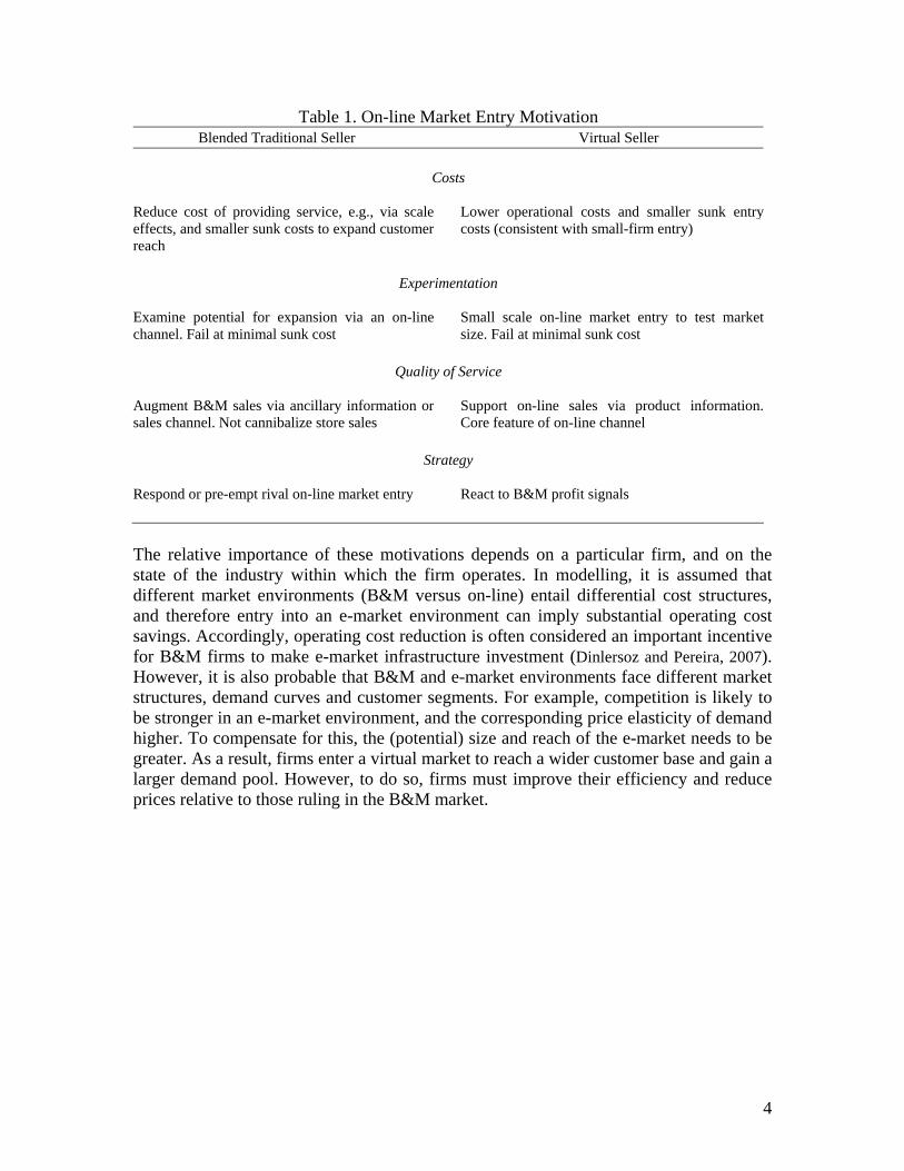
Table 1. On-line Market Entry Motivation Blended Traditional Seller Virtual Seller

Costs

Reduce cost of providing service, e.g., via scaleeffects, and smaller sunk costs to expand customerreach

Lower operational costs and smaller sunk entry costs (consistent with small-firm entry)

Experimentation

Examine potential for expansion via an on-linechannel. Fail at minimal sunk cost

Small scale on-line market entry to test market size. Fail at minimal sunk cost

Quality of Service

Augment B&M sales via ancillary information orsales channel. Not cannibalize store sales

Support on-line sales via product information. Core feature of on-line channel

Strategy

Respond or pre-empt rival on-line market entry React to B&M profit signals The relative importance of these motivations depends on a particular firm, and on the state of the industry within which the firm operates. In modelling, it is assumed that different market environments (B&M versus on-line) entail differential cost structures, and therefore entry into an e-market environment can imply substantial operating cost savings. Accordingly, operating cost reduction is often considered an important incentive for B&M firms to make e-market infrastructure investment (Dinlersoz and Pereira, 2007). However, it is also probable that B&M and e-market environments face different market structures, demand curves and customer segments. For example, competition is likely to be stronger in an e-market environment, and the corresponding price elasticity of demand higher. To compensate for this, the (potential) size and reach of the e-market needs to be greater. As a result, firms enter a virtual market to reach a wider customer base and gain a larger demand pool. However, to do so, firms must improve their efficiency and reduce prices relative to those ruling in the B&M market.

5

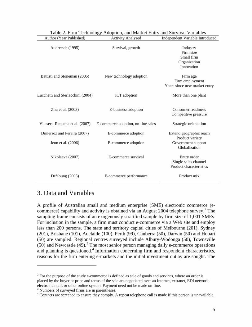
Table 2. Firm Technology Adoption, and Market Entry and Survival Variables Author (Year Published) Activity Analysed Independent Variable Introduced

Audretsch (1995) Survival, growth Industry

Firm size Small firm Organization Innovation

Battisti and Stoneman (2005) New technology adoption Firm age Firm employment Years since new market entry

Lucchetti and Sterlacchini (2004) ICT adoption More than one plant

Zhu et al. (2003) E-business adoption Consumer readiness Competitive pressure

Vilaseca-Requena et al. (2007) E-commerce adoption, on-line sales Strategic orientation

Dinlersoz and Pereira (2007) E-commerce adoption Extend geographic reach Product variety

Jeon et al. (2006) E-commerce adoption Government support Globalization

Nikolaeva (2007) E-commerce survival Entry order Single sales channel Product characteristics

DeYoung (2005) E-commerce performance Product mix

3. Data and Variables A profile of Australian small and medium enterprise (SME) electronic commerce (e-commerce) capability and activity is obtained via an August 2004 telephone survey.2 The sampling frame consists of an exogenously stratified sample by firm size of 1,001 SMEs. For inclusion in the sample, a firm must conduct e-commerce via a Web site and employ less than 200 persons. The state and territory capital cities of Melbourne (201), Sydney (201), Brisbane (101), Adelaide (100), Perth (99), Canberra (50), Darwin (50) and Hobart (50) are sampled. Regional centres surveyed include Albury-Wodonga (50), Townsville (50) and Newcastle (49).3 The most senior person managing daily e-commerce operations and planning is questioned.4 Information concerning firm and respondent characteristics, reasons for the firm entering e-markets and the initial investment outlay are sought. The

2 For the purpose of the study e-commerce is defined as sale of goods and services, where an order is placed by the buyer or price and terms of the sale are negotiated over an Internet, extranet, EDI network, electronic mail, or other online system. Payment need not be made on-line. 3 Numbers of surveyed firms are in parentheses. 4 Contacts are screened to ensure they comply. A repeat telephone call is made if this person is unavailable.

6

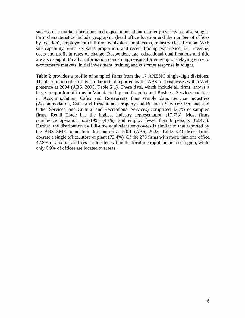
success of e-market operations and expectations about market prospects are also sought. Firm characteristics include geographic (head office location and the number of offices by location), employment (full-time equivalent employees), industry classification, Web site capability, e-market sales proportion, and recent trading experience, i.e., revenue, costs and profit in rates of change. Respondent age, educational qualifications and title are also sought. Finally, information concerning reasons for entering or delaying entry to e-commerce markets, initial investment, training and customer response is sought. Table 2 provides a profile of sampled firms from the 17 ANZSIC single-digit divisions. The distribution of firms is similar to that reported by the ABS for businesses with a Web presence at 2004 (ABS, 2005, Table 2.1). These data, which include all firms, shows a larger proportion of firms in Manufacturing and Property and Business Services and less in Accommodation, Cafes and Restaurants than sample data. Service industries (Accommodation, Cafes and Restaurants; Property and Business Services; Personal and Other Services; and Cultural and Recreational Services) comprised 42.7% of sampled firms. Retail Trade has the highest industry representation (17.7%). Most firms commence operation post-1995 (40%), and employ fewer than 6 persons (62.4%). Further, the distribution by full-time equivalent employees is similar to that reported by the ABS SME population distribution at 2001 (ABS, 2002, Table 3.4). Most firms operate a single office, store or plant (72.4%). Of the 276 firms with more than one office, 47.8% of auxiliary offices are located within the local metropolitan area or region, while only 6.9% of offices are located overseas.

7

Table 3. Sample Firm Characteristics

Sample (%) ABS (%) ANZSIC single-digit division

Retail trade 17.7 14.2 Accommodation, cafes and restaurants 16.8 4.1 Property and business services 10.5 24.0 Personal and other services 9.2 7.4 Manufacturing 6.7 12.5 Transport and storage 6.6 4.5 Cultural and recreational services 6.2 6.2 Finance and insurance 5.6 2.5 Wholesale trade 5.1 9.1 Construction 4.7 9.4 Other 10.9 6.1

Commenced operation

Prior to 1955 5.0 - 1955–1964 3.1 - 1965–1974 6.7 - 1975–1984 17.2 - 1985–1994 28.0 - 1995–2004 40.0 -

Full-time equivalent employees

1–4 57.7 63.9 5–19 29.7 29.3 20–99 11.8 6.2 100–199 0.8 0.6

Offices, stores or plants

1 72.4 - 2–5 21.9 - 6–10 3.8 - > 10 1.9 -

Auxiliary office location Number

Local metropolitan area or region 132 47.8 - Intrastate 96 34.8 - Interstate 108 39.1 - Overseas 19 6.9 -

Note. A dash indicates data is not available. Auxiliary office location applies to firms with more than one office. Source. ABS (2005) Table 2.1, businesses with Web presence. ABS (2002) Table 3.4, employer size group by industry division

8

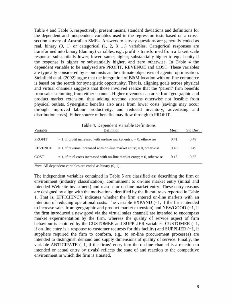
Table 4 and Table 5, respectively, present means, standard deviations and definitions for the dependent and independent variables used in the regression tests based on a cross-section survey of Australian SMEs. Answers to survey questions are generally coded as real, binary (0, 1) or categorical (1, 2, 3 …) variables. Categorical responses are transformed into binary (dummy) variables, e.g., profit is transformed from a Likert scale response: substantially lower; lower; same; higher; substantially higher to equal unity if the response is higher or substantially higher, and zero otherwise. In Table 4 the dependent variable to be analysed are PROFIT, REVENUE and COST. These variables are typically considered by economists as the ultimate objectives of agents’ optimisation. Steinfield et al. (2002) argue that the integration of B&M location with on-line commerce is based on the search for synergistic opportunity. That is, aligning goals across physical and virtual channels suggests that those involved realize that the ‘parent’ firm benefits from sales stemming from either channel. Higher revenues can arise from geographic and product market extension, thus adding revenue streams otherwise not feasible from physical outlets. Synergistic benefits also arise from lower costs (savings may occur through improved labour productivity, and reduced inventory, advertising and distribution costs). Either source of benefits may flow through to PROFIT.

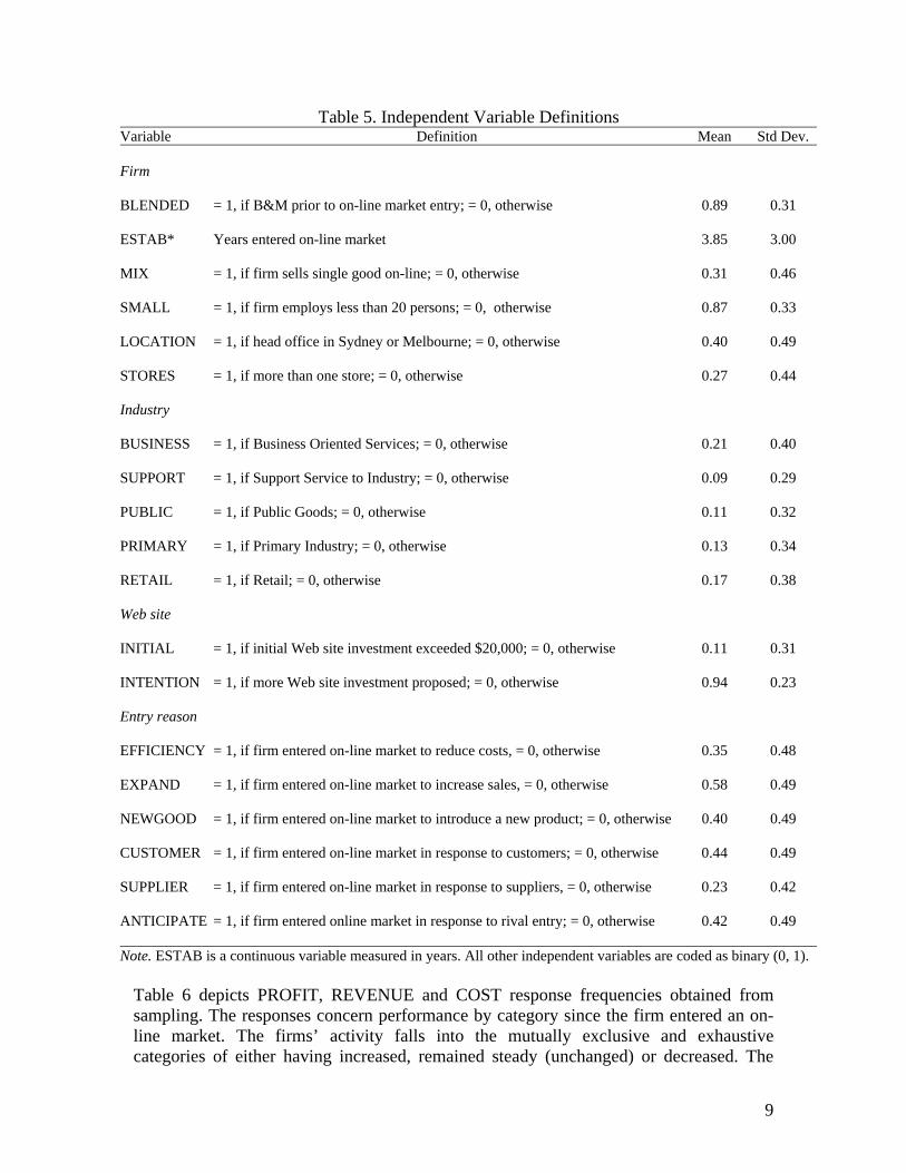
Table 4. Dependent Variable Definitions Variable Definition Mean Std Dev. PROFIT = 1, if profit increased with on-line market entry; = 0, otherwise 0.41 0.49 REVENUE = 1, if revenue increased with on-line market entry; = 0, otherwise 0.46 0.49 COST = 1, if total costs increased with on-line market entry; = 0, otherwise 0.15 0.35 Note. All dependent variables are coded as binary (0, 1). The independent variables contained in Table 5 are classified as: describing the firm or environment (industry classification), commitment to on-line market entry (initial and intended Web site investment) and reason for on-line market entry. These entry reasons are designed by align with the motivations identified by the literature as reported in Table 1. That is, EFFICIENCY indicates whether the firm entered on-line markets with an intention of reducing operational costs. The variable EXPAND (=1, if the firm intended to increase sales from geographic and product market extension) and NEWGOOD (=1, if the firm introduced a new good via the virtual sales channel) are intended to encompass market experimentation by the firm, whereas the quality of service aspect of firm behaviour is captured by the CUSTOMER and SUPPLIER variables. CUSTOMER (=1, if on-line entry is a response to customer requests for this facility) and SUPPLIER (=1, if suppliers required the firm to conform, e.g., to on-line procurement processes) are intended to distinguish demand and supply dimensions of quality of service. Finally, the variable ANTICIPATE (=1, if the firms’ entry into the on-line channel is a reaction to intended or actual entry by rivals) reflects the state of and reaction to the competitive environment in which the firm is situated.

9

Table 5. Independent Variable Definitions Variable Definition Mean Std Dev. Firm BLENDED = 1, if B&M prior to on-line market entry; = 0, otherwise 0.89 0.31 ESTAB* Years entered on-line market 3.85 3.00 MIX = 1, if firm sells single good on-line; = 0, otherwise 0.31 0.46 SMALL = 1, if firm employs less than 20 persons; = 0, otherwise 0.87 0.33 LOCATION = 1, if head office in Sydney or Melbourne; = 0, otherwise 0.40 0.49 STORES = 1, if more than one store; = 0, otherwise 0.27 0.44 Industry BUSINESS = 1, if Business Oriented Services; = 0, otherwise 0.21 0.40 SUPPORT = 1, if Support Service to Industry; = 0, otherwise 0.09 0.29 PUBLIC = 1, if Public Goods; = 0, otherwise 0.11 0.32 PRIMARY = 1, if Primary Industry; = 0, otherwise 0.13 0.34 RETAIL = 1, if Retail; = 0, otherwise 0.17 0.38 Web site INITIAL = 1, if initial Web site investment exceeded $20,000; = 0, otherwise 0.11 0.31 INTENTION = 1, if more Web site investment proposed; = 0, otherwise 0.94 0.23 Entry reason EFFICIENCY = 1, if firm entered on-line market to reduce costs, = 0, otherwise 0.35 0.48 EXPAND = 1, if firm entered on-line market to increase sales, = 0, otherwise 0.58 0.49 NEWGOOD = 1, if firm entered on-line market to introduce a new product; = 0, otherwise 0.40 0.49 CUSTOMER = 1, if firm entered on-line market in response to customers; = 0, otherwise 0.44 0.49 SUPPLIER = 1, if firm entered on-line market in response to suppliers, = 0, otherwise 0.23 0.42 ANTICIPATE = 1, if firm entered online market in response to rival entry; = 0, otherwise 0.42 0.49 Note. ESTAB is a continuous variable measured in years. All other independent variables are coded as binary (0, 1).

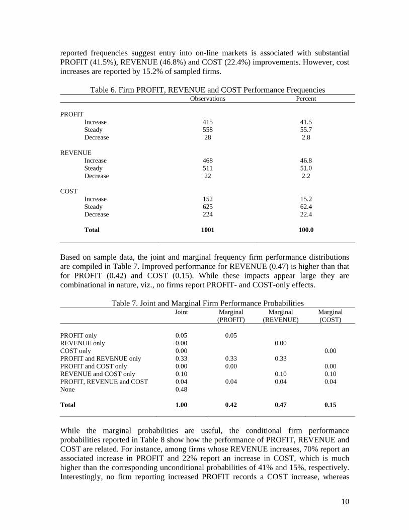
Table 6 depicts PROFIT, REVENUE and COST response frequencies obtained from sampling. The responses concern performance by category since the firm entered an on-line market. The firms’ activity falls into the mutually exclusive and exhaustive categories of either having increased, remained steady (unchanged) or decreased. The

10

reported frequencies suggest entry into on-line markets is associated with substantial PROFIT (41.5%), REVENUE (46.8%) and COST (22.4%) improvements. However, cost increases are reported by 15.2% of sampled firms.

Table 6. Firm PROFIT, REVENUE and COST Performance Frequencies Observations Percent PROFIT

Increase 415 41.5 Steady 558 55.7 Decrease 28 2.8

REVENUE

Increase 468 46.8 Steady 511 51.0 Decrease 22 2.2

COST

Increase 152 15.2 Steady 625 62.4 Decrease 224 22.4 Total 1001 100.0

Based on sample data, the joint and marginal frequency firm performance distributions are compiled in Table 7. Improved performance for REVENUE (0.47) is higher than that for PROFIT (0.42) and COST (0.15). While these impacts appear large they are combinational in nature, viz., no firms report PROFIT- and COST-only effects.

Table 7. Joint and Marginal Firm Performance Probabilities Joint

Marginal (PROFIT)

Marginal (REVENUE)

Marginal (COST)

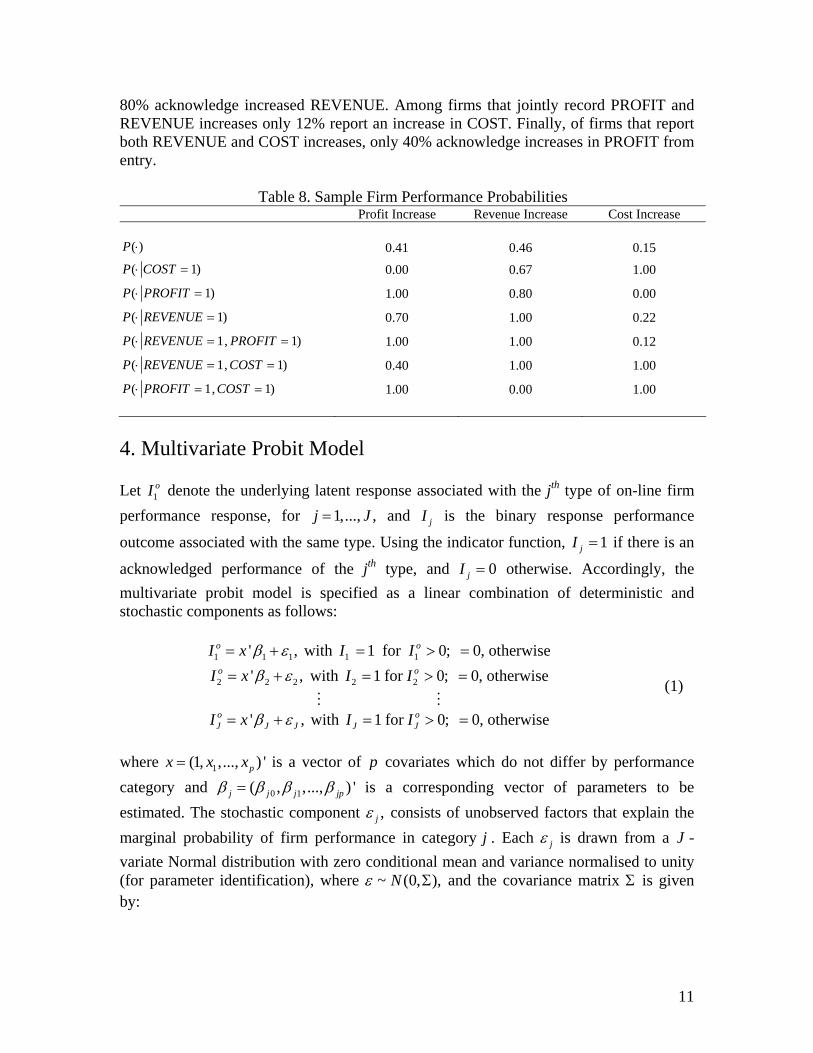
PROFIT only 0.05 0.05 REVENUE only 0.00 0.00 COST only 0.00 0.00 PROFIT and REVENUE only 0.33 0.33 0.33 PROFIT and COST only 0.00 0.00 0.00 REVENUE and COST only 0.10 0.10 0.10 PROFIT, REVENUE and COST 0.04 0.04 0.04 0.04 None 0.48 Total 1.00 0.42 0.47 0.15 While the marginal probabilities are useful, the conditional firm performance probabilities reported in Table 8 show how the performance of PROFIT, REVENUE and COST are related. For instance, among firms whose REVENUE increases, 70% report an associated increase in PROFIT and 22% report an increase in COST, which is much higher than the corresponding unconditional probabilities of 41% and 15%, respectively. Interestingly, no firm reporting increased PROFIT records a COST increase, whereas

11

80% acknowledge increased REVENUE. Among firms that jointly record PROFIT and REVENUE increases only 12% report an increase in COST. Finally, of firms that report both REVENUE and COST increases, only 40% acknowledge increases in PROFIT from entry.

Table 8. Sample Firm Performance Probabilities Profit Increase Revenue Increase Cost Increase

( )⋅P 0.41 0.46 0.15 ( 1)⋅ =P COST 0.00 0.67 1.00

( 1)⋅ =P PROFIT 1.00 0.80 0.00

( 1)⋅ =P REVENUE 0.70 1.00 0.22

( 1, 1)⋅ = =P REVENUE PROFIT 1.00 1.00 0.12

( 1, 1)⋅ = =P REVENUE COST 0.40 1.00 1.00

( 1, 1)⋅ = =P PROFIT COST 1.00 0.00 1.00 4. Multivariate Probit Model Let 1

oI denote the underlying latent response associated with the jth type of on-line firm performance response, for 1,..., ,=j J and jI is the binary response performance

outcome associated with the same type. Using the indicator function, 1=jI if there is an

acknowledged performance of the jth type, and 0=jI otherwise. Accordingly, the multivariate probit model is specified as a linear combination of deterministic and stochastic components as follows:

1 1 1' ,β ε= +oI x with 1 11 for 0; 0, otherwise= > =oI I

2 2 2' ,β ε= +oI x with 2 21 for 0; 0, otherwise= > =oI I M M

' ,β ε= +oJ J JI x with 1 for 0; 0, otherwise= > =o

J JI I

(1)

where 1(1, ,..., ) '= px x x is a vector of p covariates which do not differ by performance category and 0 1( , ,..., ) 'β β β β=j j j jp is a corresponding vector of parameters to be estimated. The stochastic component ,ε j consists of unobserved factors that explain the marginal probability of firm performance in category j . Each ε j is drawn from a J -variate Normal distribution with zero conditional mean and variance normalised to unity (for parameter identification), where ~ (0, ),ε ΣN and the covariance matrix Σ is given by:

12

12 1J

21 2J

J1 J2

11

1

ρ ρρ ρ

ρ ρ

⎡ ⎤⎢ ⎥⎢ ⎥Σ =⎢ ⎥⎢ ⎥⎣ ⎦

L

L

M M O M

L

. (2)

The off-diagonal elements ρsj represent unobserved correlations between the stochastic component of the sth and the jth performance category. Because of covariance symmetry ρ ρ=sj js . From the multivariable probit model formulation, the univariate marginal performance probability by category is:

'1Pr( 1 ) ( ) for 1,...,β= = Φ =j j jj

I x x j J (3) where 1( )Φ ⋅ is the standard Normal distribution function. Moreover, the bivariate joint probabilities are given by:

' '2

' '2

' '2

Pr( 1, 1 , ) ( , ; )

Pr( 1, 0 , ) ( , ; ), and

Pr( 0, 0 , ) ( , ; )

β β ρ

β β ρ

β β ρ

= = = Φ

= = = Φ − −

= = = Φ − −

i j j i i j j iji

i j j i i j j iji

i j j i i j j iji

I I x x x x

I I x x x x

I I x x x x

(4)

where , , , ;= Π ≠i j R C i j and 2 1 2 12( , ; )γΦ z z is the cumulative distribution function of standard bivariate Normal distribution with 12γ the correlation coefficient of the two univariate random elements 1z and 2z . The trivariate joint probabilities (with , , , , ; , , )= Π ≠ ≠ ≠i j k R C i j i k j k ) are:

' ' '3

' ' '3

' ' '3

Pr( 1, 1, 1 , , ) ( , , ; , , ),

Pr( 1, 1, 0 , , ) ( , , ; , , ),

Pr( 1, 0, 0 , , ) ( , , ; , , ), and

Pr(

β β β ρ ρ ρ

β β β ρ ρ ρ

β β β ρ ρ ρ

= = = = Φ

= = = = Φ − − −

= = = = Φ − − − −

=

i j k j k i i j j k k ij ik jki



i

I I I x x x x x x

I I I x x x x x x

I I I x x x x x x

I ' ' '30, 0, 0 , , ) ( , , ; , , )β β β ρ ρ ρ= = = Φ − − −j k j k i i j j k k ij ik jki

I I x x x x x x

(5)

where 3 1 2 3 12 13 23( , , ; , )γ γ γΦ z z z is the cumulative distribution function of standard trivariate Normal distribution with γ st the correlation coefficient of two of the three univariate random elements sz and tz ( , 1, 2,3; )= ≠s t s t . The structure of the corresponding conditional probabilities is;

13

' ' '3

' '2

' ' '3

' '2

'3

( , , ; , , )Pr( 1 1, 1; , , ) ,

( , ; )

( , , ; , , )Pr( 1 0, 0; , , ) ,

( , ; )

(Pr( 0, 0 1; , , )

β β β ρ ρ ρβ β ρ

β β β ρ ρ ρβ β ρ

Φ= = = =

Φ

Φ − − − −= = = =

Φ − −

Φ −= = = =

i i j j k k ij ik jki j k i j k

i i j j ij

i i j j k k ij ik jki j k i j k

j j k k jk

ii j k i j k

x x xI I I x x x

x x

x x xI I I x x x

x x

xI I I x x x

' '

'1

' '2

'1

, , ; , , ), and

( )

( , ; )Pr( 1 1; , ) .

( )

β β β ρ ρ ρβ

β β ρβ

− − −

Φ

Φ= = =

Φ

i j j k k ij ik jk

k k

i i j j iji j i j

j j

x xx

x xI I x x

x

(6)

Given an . . .i i d sample of J firms and conditional on firm heterogeneity, the multivariable probit model is estimated by maximising the log-likelihood function:

1 1 1

1 0 0 0

( ) ( , , ) log(Prob( , , , , )),Π Π= = = =

= = = =∑∑∑∑N

s R C s Rs Css i j k

Log L h i j k I i I j I k x x x

where

1 if firm chooses ( , , )( , , )

0 otherwise. Π = = =⎧

= ⎨⎩

R Cs

s I i I j I kh i j k

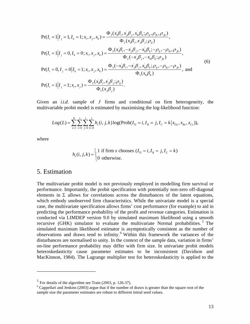
5. Estimation The multivariate probit model is not previously employed in modelling firm survival or performance. Importantly, the probit specification with potentially non-zero off-diagonal elements in Σ allows for correlations across the disturbances of the latent equations, which embody unobserved firm characteristics. While the univariate model is a special case, the multivariate specification allows firms’ cost performance (for example) to aid in predicting the performance probability of the profit and revenue categories. Estimation is conducted via LIMDEP version 9.0 by simulated maximum likelihood using a smooth recursive (GHK) simulator to evaluate the multivariate Normal probabilities. 5 The simulated maximum likelihood estimator is asymptotically consistent as the number of observations and draws tend to infinity.6 Within this framework the variances of the disturbances are normalised to unity. In the context of the sample data, variation in firms’ on-line performance probability may differ with firm size. In univariate probit models heteroskedasticity cause parameter estimates to be inconsistent (Davidson and MacKinnon, 1984). The Lagrange multiplier test for heteroskedasticity is applied to the

5 For details of the algorithm see Train (2003, p. 126-37). 6 Cappellari and Jenkins (2003) argue that if the number of draws is greater than the square root of the sample size the parameter estimates are robust to different initial seed values.

14

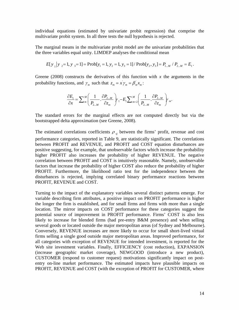
individual equations (estimated by univariate probit regression) that comprise the multivariate probit system. In all three tests the null hypothesis is rejected. The marginal means in the multivariate probit model are the univariate probabilities that the three variables equal unity. LIMDEP analyses the conditional mean

2 3 1 2 3 2 3 1... 2... 11[ 1, 1] Prob[ 1, 1, 1] / Prob[ , ] /= = = = = = = =M ME y y y y y y y y P P E .

Greene (2008) constructs the derivatives of this function with x the arguments in the probability functions, and γ m such that ' 'γ β= =m m m mz x x :

2... 2...11 1 2

2... 2...

1 1. . .γ γ=

⎛ ⎞ ⎛ ⎞∂ ∂∂= −⎜ ⎟ ⎜ ⎟∂ ∂ ∂⎝ ⎠ ⎝ ⎠∑ ∑M MM M

mm mM m M m

P PE Ex P z P z

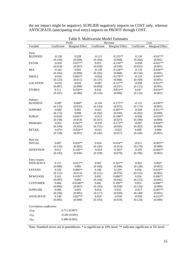
The standard errors for the marginal effects are not computed directly but via the bootstrapped delta approximation (see Greene, 2008). The estimated correlations coefficients ρ sj between the firms’ profit, revenue and cost performance categories, reported in Table 9, are statistically significant. The correlations between PROFIT and REVENUE, and PROFIT and COST equation disturbances are positive suggesting, for example, that unobservable factors which increase the probability higher PROFIT also increases the probability of higher REVENUE. The negative correlation between PROFIT and COST is intuitively reasonable. Namely, unobservable factors that increase the probability of higher COST also reduce the probability of higher PROFIT. Furthermore, the likelihood ratio test for the independence between the disturbances is rejected, implying correlated binary performance reactions between PROFIT, REVENUE and COST. Turning to the impact of the explanatory variables several distinct patterns emerge. For variable describing firm attributes, a positive impact on PROFIT performance is higher the longer the firm is established, and for small firms and firms with more than a single location. The mirror impacts on COST performance for these categories suggest the potential source of improvement in PROFIT performance. Firms’ COST is also less likely to increase for blended firms (had pre-entry B&M presence) and when selling several goods or located outside the major metropolitan areas (of Sydney and Melbourne). Conversely, REVENUE increases are more likely to occur for small short-lived virtual firms selling a single good outside major metropolitan areas. Improved performance, for all categories with exception of REVENUE for intended investment, is reported for the Web site investment variables. Finally, EFFICIENCY (cost reduction), EXPANSION (increase geographic market coverage), NEWGOOD (introduce a new product), CUSTOMER (respond to customer request) motivations significantly impact on post-entry on-line market performance. The estimated impacts have plausible impacts on PROFIT, REVENUE and COST (with the exception of PROFIT for CUSTOMER, where

15

the net impact might be negative). SUPLIER negatively impacts on COST only, whereas ANTICIPATE (anticipating rival entry) impacts on PROFIT through COST.

Table 9. Multivariate Model Estimates Profit Revenue Cost

Variable Coefficient Marginal Effect Coefficient Marginal Effect Coefficient Marginal Effect Firm BLENDED -0.158

(0.159) 0.028

(0.028) -0.113 (0.164)

-0.225** (0.068)

-0.116 (0.204)

-0.037** (0.001)

ESTAB -0.028 (0.014)

0.027** (0.007)

0.015 (0.018)

-0.156** (0.036)

-0.058 (0.023)

-0.021** (0.001)

MIX -0.162 (0.103)

0.002 (0.009)

-0.128 (0.105)

-0.228** (0.068)

-0.116 (0.134)

-0.036** (0.001)

SMALL -0.016 (0.123)

0.065** (0.011)

-0.024 (0.137)

-0.278** (0.066)

-0.119 (0.169)

-0.045** (0.001)

LOCATION -0.016 (0.087)

0.010 (0.008)

-0.087 (0.094)

-0.127** (0.037)

-0.058 (0.113)

-0.012** (0.001)

STORES 0.111 (0.107)

0.030** (0.006)

0.016 (0.114)

-0.031** (0.006)

0.047 (0.135)

-0.016** (0.001)

Industry BUSINESS -0.087

(0.133) 0.060* (0.032)

-0.134 (0.143)

-0.175** (0.051)

-0.112 (0.173)

-0.030** (0.001)

SUPPORT -0.082 (0.172)

0.001 0.008

-0.021 (0.182)

-0.087** (0.030)

-0.028 (0.202)

-0.011** (0.000)

PUBLIC -0.0181 (0.158)

0.042** (0.014)

-0.013 (0.167)

-0.108** (0.027)

-0.056 (0.198)

-0.019** (0.000)

PRIMARY -0.055 (0.144)

0.042** (0.020)

-0.070 (0.151)

-0.172** (0.043)

-0.097 (0.203)

-0.026** (0.000)

RETAIL -0.079 (0.128)

-0.026** (0.001)

-0.021 (0.142)

-0.025 (0.017)

0.008 (0.166)

0.000 (0.001)

Web site INITIAL 0.067

(0.133) 0.020** (0.002)

0.024 (0.145)

0.014** (0.013)

-0.011 (0.179)

-0.003** (0.000)

INTENTION 0.012 (0.145)

0.128** (0.036)

-0.054 (0.158)

-0.365* (0.079)

-0.195 (0.196)

-0.064** (0.001)

Entry reason EFFICIENCY 0.157

(0.098) 0.012** 0.005

0.062 (0.106)

0.101** (0.048)

-0.001 (0.128)

0.002* (0.001)

EXPAND 0.336 (0.115)

0.080** (0.013)

0.196 (0.121)

0.129* (0.076)

0.034 (0.135)

0.010** (0.002)

NEWGOOD 0.161 (0.097)

0.019** 0.003

0.091 (0.104)

0.088** (0.042)

0.026 (0.123)

0.006** (0.001)

CUSTOMER 0.066 (0.096)

-0.0146** (0.007)

0.041 (0.105)

0.109** (0.038)

0.025 (0.124)

0.008** (0.000)

SUPPLIER 0.096 (0.104)

0.003 (0.005)

0.054 (0.117)

0.023 (0.020)

-0.017 (0.140)

-0.007** (0.001)

ANTICIPATE 0.149 (0.095)

0.037** (0.008)

0.029 (0.103)

-0.018 (0.019)

-0.058 (0.124)

-0.013** (0.000)

Correlation coefficients

RρΠ 0.711 (0.007)

CρΠ -0.265 (0.001)

RCρ 0.490 (0.005) Note. Standard errors are in parentheses. * is significant at 10% level. ** indicates significant at 5% level.

16

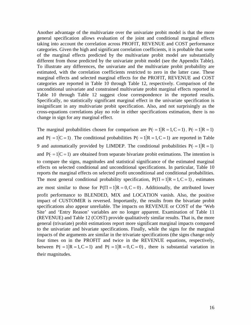
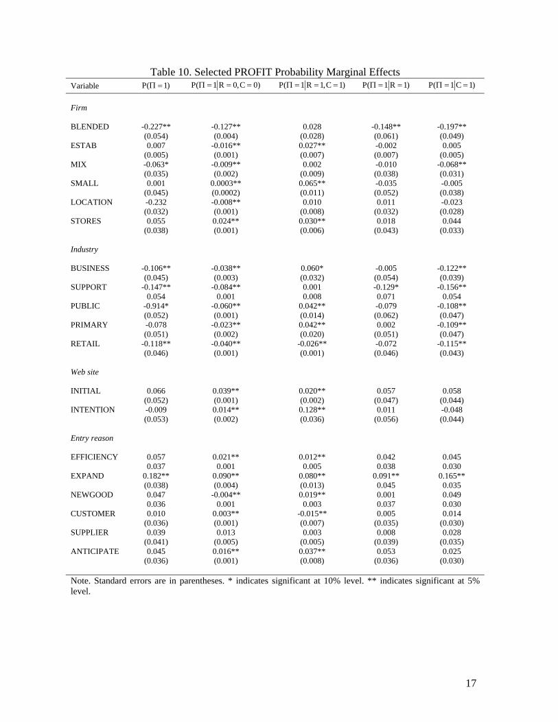
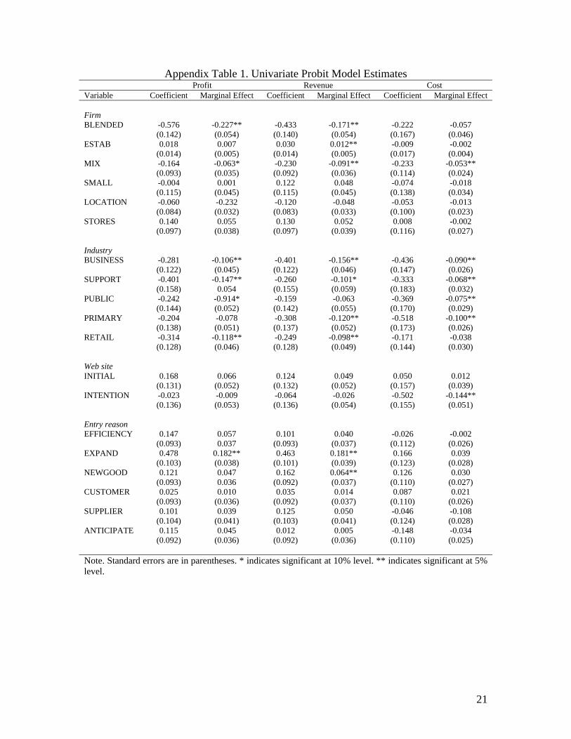
Another advantage of the multivariate over the univariate probit model is that the more general specification allows evaluation of the joint and conditional marginal effects taking into account the correlation across PROFIT, REVENUE and COST performance categories. Given the high and significant correlation coefficients, it is probable that some of the marginal effects predicted by the multivariate probit model are substantially different from those predicted by the univariate probit model (see the Appendix Table). To illustrate any differences, the univariate and the multivariate probit probability are estimated, with the correlation coefficients restricted to zero in the latter case. These marginal effects and selected marginal effects for the PROFIT, REVENUE and COST categories are reported in Table 10 through Table 12, respectively. Comparison of the unconditional univariate and constrained multivariate probit marginal effects reported in Table 10 through Table 12 suggest close correspondence in the reported results. Specifically, no statistically significant marginal effect in the univariate specification is insignificant in any multivariate probit specification. Also, and not surprisingly as the cross-equations correlations play no role in either specifications estimation, there is no change in sign for any marginal effect. The marginal probabilities chosen for comparison are P( 1 R 1,C 1)⋅ = = = , P( 1 R 1)⋅ = =

and P( 1 C 1)⋅ = = . The conditional probabilities P( 1 R 1,C 1)⋅ = = = are reported in Table

9 and automatically provided by LIMDEP. The conditional probabilities P( 1 R 1)⋅ = =

and P( 1 C 1)⋅ = = are obtained from separate bivariate probit estimations. The intention is to compare the signs, magnitudes and statistical significance of the estimated marginal effects on selected conditional and unconditional specifications. In particular, Table 10 reports the marginal effects on selected profit unconditional and conditional probabilities. The most general conditional probability specification, P( 1 R 1,C 1)Π = = = , estimates

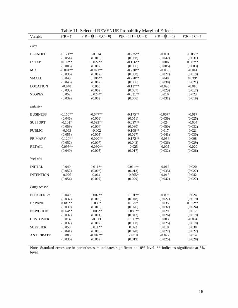
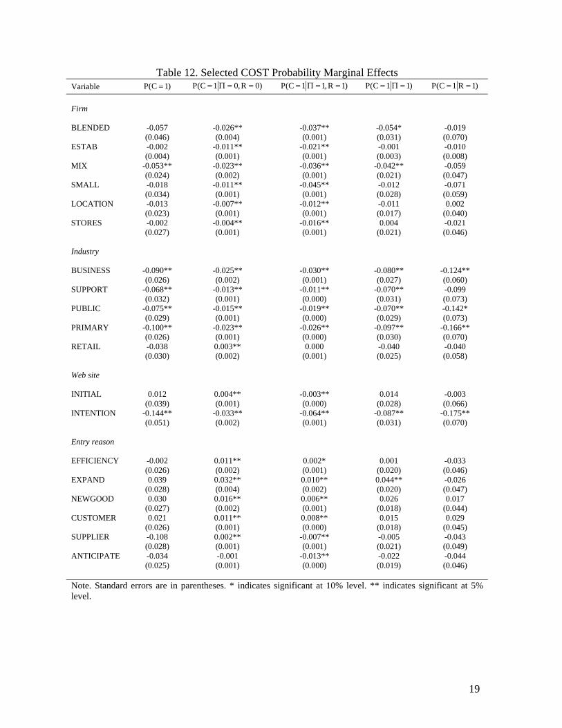
are most similar to those for P( 1 R 0,C 0)Π = = = . Additionally, the attributed lower profit performance to BLENDED, MIX and LOCATION vanish. Also, the positive impact of CUSTOMER is reversed. Importantly, the results from the bivariate probit specifications also appear unreliable. The impacts on REVENUE or COST of the ‘Web Site’ and ‘Entry Reason’ variables are no longer apparent. Examination of Table 11 (REVENUE) and Table 12 (COST) provide qualitatively similar results. That is, the more general (trivariate) probit estimations report more significant marginal impacts compared to the univariate and bivariate specifications. Finally, while the signs for the marginal impacts of the arguments are similar in the trivariate specifications (the signs change only four times on in the PROFIT and twice in the REVENUE equations, respectively, between P( 1 R 1,C 1)⋅ = = = and P( 1 R 0,C 0)⋅ = = = , there is substantial variation in their magnitudes.

17

Table 10. Selected PROFIT Probability Marginal Effects Variable P( 1)Π = P( 1 R 0,C 0)Π = = = P( 1 R 1,C 1)Π = = = P( 1 R 1)Π = = P( 1 C 1)Π = = Firm BLENDED -0.227**

(0.054) -0.127** (0.004)

0.028 (0.028)

-0.148** (0.061)

-0.197** (0.049)

ESTAB 0.007 (0.005)

-0.016** (0.001)

0.027** (0.007)

-0.002 (0.007)

0.005 (0.005)

MIX -0.063* (0.035)

-0.009** (0.002)

0.002 (0.009)

-0.010 (0.038)

-0.068** (0.031)

SMALL 0.001 (0.045)

0.0003** (0.0002)

0.065** (0.011)

-0.035 (0.052)

-0.005 (0.038)

LOCATION -0.232 (0.032)

-0.008** (0.001)

0.010 (0.008)

0.011 (0.032)

-0.023 (0.028)

STORES 0.055 (0.038)

0.024** (0.001)

0.030** (0.006)

0.018 (0.043)

0.044 (0.033)

Industry BUSINESS -0.106**

(0.045) -0.038** (0.003)

0.060* (0.032)

-0.005 (0.054)

-0.122** (0.039)

SUPPORT -0.147** 0.054

-0.084** 0.001

0.001 0.008

-0.129* 0.071

-0.156** 0.054

PUBLIC -0.914* (0.052)

-0.060** (0.001)

0.042** (0.014)

-0.079 (0.062)

-0.108** (0.047)

PRIMARY -0.078 (0.051)

-0.023** (0.002)

0.042** (0.020)

0.002 (0.051)

-0.109** (0.047)

RETAIL -0.118** (0.046)

-0.040** (0.001)

-0.026** (0.001)

-0.072 (0.046)

-0.115** (0.043)


(0.052) 0.039** (0.001)

0.020** (0.002)

0.057 (0.047)

0.058 (0.044)

INTENTION -0.009 (0.053)

0.014** (0.002)

0.128** (0.036)

0.011 (0.056)

-0.048 (0.044)


0.037 0.021** 0.001

0.012** 0.005

0.042 0.038

0.045 0.030

EXPAND 0.182** (0.038)

0.090** (0.004)

0.080** (0.013)

0.091** 0.045

0.165** 0.035

NEWGOOD 0.047 0.036

-0.004** 0.001

0.019** 0.003

0.001 0.037

0.049 0.030

CUSTOMER 0.010 (0.036)

0.003** (0.001)

-0.015** (0.007)

0.005 (0.035)

0.014 (0.030)

SUPPLIER 0.039 (0.041)

0.013 (0.005)

0.003 (0.005)

0.008 (0.039)

0.028 (0.035)


0.016** (0.001)

0.037** (0.008)

0.053 (0.036)

0.025 (0.030)

Note. Standard errors are in parentheses. * indicates significant at 10% level. ** indicates significant at 5% level.

18

Table 11. Selected REVENUE Probability Marginal Effects Variable P(R 1)= P(R 1 0,C 0)= Π = = P(R 1 1,C 1)= Π = = P(R 1 1)= Π = P(R 1 C 1)= = Firm BLENDED -0.171**

(0.054) -0.014 (0.018)

-0.225** (0.068)

-0.001 (0.042)

-0.053* (0.031)

ESTAB 0.012** (0.005)

0.027** (0.002)

-0.156** (0.036)

0.006 (0.005)

0.007** (0.003)

MIX -0.091** (0.036)

-0.021** (0.002)

-0.228** (0.068)

-0.035 (0.027)

-0.014 (0.019)

SMALL 0.048 (0.045)

0.106** (0.002)

-0.278** (0.066)

0.040 (0.038)

0.039* (0.021)

LOCATION -0.048 (0.033)

0.003 (0.002)

-0.127** (0.037)

-0.026 (0.023)

-0.016 (0.017)

STORES 0.052 (0.039)

0.024** (0.002)

-0.031** (0.006)

0.016 (0.031)

0.023 (0.019)


(0.046) -0.047** (0.008)

-0.175** (0.051)

-0.067* (0.039)

-0.017 (0.025)

SUPPORT -0.101* (0.059)

-0.035** (0.004)

-0.087** (0.030)

0.024 (0.050)

-0.004 (0.032)

PUBLIC -0.063 (0.055)

-0.002 (0.005)

-0.108** (0.027)

0.017 (0.043)

0.021 (0.030)

PRIMARY -0.120** (0.052)

-0.020** (0.007)

-0.172** (0.043)

-0.054 (0.036)

0.008 (0.029)

RETAIL -0.098** (0.049)

-0.030** (0.005)

-0.025 (0.017)

-0.005 (0.032)

-0.020 (0.026)


(0.052) 0.011** (0.005)

0.014** (0.013)

-0.012 (0.033)

0.020 (0.027)

INTENTION -0.026 (0.054)

0.064 (0.007)

-0.365* (0.079)

-0.017 (0.042)

0.042 (0.027)


(0.037) 0.002** (0.000)

0.101** (0.048)

-0.006 (0.027)

0.024 (0.019)

EXPAND 0.181** (0.039)

0.030* (0.016)

0.129* (0.076)

0.035 (0.032)

0.072** (0.024)

NEWGOOD 0.064** (0.037)

0.005** (0.001)

0.088** (0.042)

0.029 (0.026)

0.017 (0.019)

CUSTOMER 0.014 (0.037)

-0.013 (0.002)

0.109** (0.038)

0.003 (0.025)

-0.004 (0.019)

SUPPLIER 0.050 (0.041)

0.011** (0.000)

0.023 (0.020)

0.018 (0.027)

0.030 (0.022)


-0.016** (0.002)

-0.018 (0.019)

-0.027 (0.025)

0.014 (0.020)


19

Table 12. Selected COST Probability Marginal Effects Variable P(C 1)= P(C 1 0,R 0)= Π = = P(C 1 1,R 1)= Π = = P(C 1 1)= Π = P(C 1 R 1)= = Firm BLENDED -0.057

(0.046) -0.026** (0.004)

-0.037** (0.001)

-0.054* (0.031)

-0.019 (0.070)

ESTAB -0.002 (0.004)

-0.011** (0.001)

-0.021** (0.001)

-0.001 (0.003)

-0.010 (0.008)

MIX -0.053** (0.024)

-0.023** (0.002)

-0.036** (0.001)

-0.042** (0.021)

-0.059 (0.047)

SMALL -0.018 (0.034)

-0.011** (0.001)

-0.045** (0.001)

-0.012 (0.028)

-0.071 (0.059)

LOCATION -0.013 (0.023)

-0.007** (0.001)

-0.012** (0.001)

-0.011 (0.017)

0.002 (0.040)

STORES -0.002 (0.027)

-0.004** (0.001)

-0.016** (0.001)

0.004 (0.021)

-0.021 (0.046)


(0.026) -0.025** (0.002)

-0.030** (0.001)

-0.080** (0.027)

-0.124** (0.060)

SUPPORT -0.068** (0.032)

-0.013** (0.001)

-0.011** (0.000)

-0.070** (0.031)

-0.099 (0.073)

PUBLIC -0.075** (0.029)

-0.015** (0.001)

-0.019** (0.000)

-0.070** (0.029)

-0.142* (0.073)

PRIMARY -0.100** (0.026)

-0.023** (0.001)

-0.026** (0.000)

-0.097** (0.030)

-0.166** (0.070)

RETAIL -0.038 (0.030)

0.003** (0.002)

0.000 (0.001)

-0.040 (0.025)

-0.040 (0.058)


(0.039) 0.004** (0.001)

-0.003** (0.000)

0.014 (0.028)

-0.003 (0.066)

INTENTION -0.144** (0.051)

-0.033** (0.002)

-0.064** (0.001)

-0.087** (0.031)

-0.175** (0.070)

Entry reason EFFICIENCY -0.002

(0.026) 0.011** (0.002)

0.002* (0.001)

0.001 (0.020)

-0.033 (0.046)

EXPAND 0.039 (0.028)

0.032** (0.004)

0.010** (0.002)

0.044** (0.020)

-0.026 (0.047)

NEWGOOD 0.030 (0.027)

0.016** (0.002)

0.006** (0.001)

0.026 (0.018)

0.017 (0.044)

CUSTOMER 0.021 (0.026)

0.011** (0.001)

0.008** (0.000)

0.015 (0.018)

0.029 (0.045)

SUPPLIER -0.108 (0.028)

0.002** (0.001)

-0.007** (0.001)

-0.005 (0.021)

-0.043 (0.049)

ANTICIPATE -0.034 (0.025)

-0.001 (0.001)

-0.013** (0.000)

-0.022 (0.019)

-0.044 (0.046)


20

6. Conclusions During the past decade there is considerable research examining firm post-entry survival and performance. These studies primarily focused, presumably due to the data available, on survival. When performance per se is addressed the indicators of ‘success’ are typically some measure output, employment, or their combination productivity. A problem with this approach is that economic theory does not suggest that firms usually pursue these goals in an optimising sense. Theory suggests that firms in conducting their operations maximise profit and revenues or, via a dual program, minimise costs. Accordingly, the modelling approach employed in this study is based on the premise that firms enter on-line markets with a view to pursuing these goals. In particular, this study addresses the questions: How do virtual firms differ in their on-line market adoption patterns? In what type of environments is post on-line market entry performance by virtual and established firms likely to succeed? What can be said about the relationship between post-entry performance and the reasons for entry? The short answer to these questions (in the context of small Australian firms) is that the reasons for entry matter for performance, and by type of performance measure. In particular, entry that seeks to reduce firm cost, expand geographic market coverage or introduce new goods, while naturally increasing costs, is associated with improved revenue and profit outcomes. Entry that is a response to customer request or supplier requirement is ambiguous in outcome. Responding to customers will increase revenue but may reduce profit. Whereas, acceding to suppliers can reduce the probability of enhanced cost-based productivity performance. Finally, strategic entry can improve profit via costs, but not revenue. Another study finding is methodologically orientated, viz., the econometric estimations clearly indicate that restrictive single or multiple equation models can provide misleading indications of the marginal impact of arguments on both conditional and unconditional probabilities of firm success factors from entry. A limitation of the analysis is that only the mapping from the reasons for entry on post-entry success is considered. A more thorough analysis would consider the impact on ‘intermediate variables’ during the traverse to these outcomes. In particular, a more thoughtful analysis might consider potential impacts on employment, prices, and the source of cost improvement, e.g., whether via advertising, inventory or distribution cost reductions. The analysis might also have addressed firms’ initial Web site capability, whether on-line market performance cannibalised B&M store sales, and the empirical magnitude and pattern of market expansion.

21

Appendix Table 1. Univariate Probit Model Estimates Profit Revenue Cost

Variable Coefficient Marginal Effect Coefficient Marginal Effect Coefficient Marginal Effect Firm BLENDED -0.576

(0.142) -0.227** (0.054)

-0.433 (0.140)

-0.171** (0.054)

-0.222 (0.167)

-0.057 (0.046)

ESTAB 0.018 (0.014)

0.007 (0.005)

0.030 (0.014)

0.012** (0.005)

-0.009 (0.017)

-0.002 (0.004)

MIX -0.164 (0.093)

-0.063* (0.035)

-0.230 (0.092)

-0.091** (0.036)

-0.233 (0.114)

-0.053** (0.024)

SMALL -0.004 (0.115)

0.001 (0.045)

0.122 (0.115)

0.048 (0.045)

-0.074 (0.138)

-0.018 (0.034)

LOCATION -0.060 (0.084)

-0.232 (0.032)

-0.120 (0.083)

-0.048 (0.033)

-0.053 (0.100)

-0.013 (0.023)

STORES 0.140 (0.097)

0.055 (0.038)

0.130 (0.097)

0.052 (0.039)

0.008 (0.116)

-0.002 (0.027)

Industry BUSINESS -0.281

(0.122) -0.106** (0.045)

-0.401 (0.122)

-0.156** (0.046)

-0.436 (0.147)

-0.090** (0.026)

SUPPORT -0.401 (0.158)

-0.147** 0.054

-0.260 (0.155)

-0.101* (0.059)

-0.333 (0.183)

-0.068** (0.032)

PUBLIC -0.242 (0.144)

-0.914* (0.052)

-0.159 (0.142)

-0.063 (0.055)

-0.369 (0.170)

-0.075** (0.029)

PRIMARY -0.204 (0.138)

-0.078 (0.051)

-0.308 (0.137)

-0.120** (0.052)

-0.518 (0.173)

-0.100** (0.026)

RETAIL -0.314 (0.128)

-0.118** (0.046)

-0.249 (0.128)

-0.098** (0.049)

-0.171 (0.144)

-0.038 (0.030)


(0.131) 0.066

(0.052) 0.124

(0.132) 0.049

(0.052) 0.050

(0.157) 0.012

(0.039) INTENTION -0.023

(0.136) -0.009 (0.053)

-0.064 (0.136)

-0.026 (0.054)

-0.502 (0.155)

-0.144** (0.051)


(0.093) 0.057 0.037

0.101 (0.093)

0.040 (0.037)

-0.026 (0.112)

-0.002 (0.026)

EXPAND 0.478 (0.103)

0.182** (0.038)

0.463 (0.101)

0.181** (0.039)

0.166 (0.123)

0.039 (0.028)

NEWGOOD 0.121 (0.093)

0.047 0.036

0.162 (0.092)

0.064** (0.037)

0.126 (0.110)

0.030 (0.027)

CUSTOMER 0.025 (0.093)

0.010 (0.036)

0.035 (0.092)

0.014 (0.037)

0.087 (0.110)

0.021 (0.026)

SUPPLIER 0.101 (0.104)

0.039 (0.041)

0.125 (0.103)

0.050 (0.041)

-0.046 (0.124)

-0.108 (0.028)


0.045 (0.036)

0.012 (0.092)

0.005 (0.036)

-0.148 (0.110)

-0.034 (0.025)


22

References ABS (2002), Small Business in Australia, Catalogue 1321.0, Australian Bureau of

Statistics, Canberra ABS (2004), Business Use of Information Technology, 2002-03, Catalogue 8129.0,

Australian Bureau of Statistics, Canberra ABS (2005), Business Use of Information Technology, 2004-05, Catalogue 8129.0,

Australian Bureau of Statistics, Canberra ABS (2006), Business Use of Information Technology, 2005-06, Catalogue 8129.0,

Australian Bureau of Statistics, Canberra Audretsch, D. (1995), ‘Innovation, Growth and Survival’, International Journal of

Industrial Organization, 13, 441-57 Battisti, G. and Stoneman, P. (2005), ‘The Intra-Firm Diffusion of New Process

Technologies’, International Journal of Industrial Organisation, 23, 1-22 Cappellari, L. and Jenkins, S. (2003), ‘Multivariate Probit Regression using Simulated

Maximum Likelihood’, Strata Journal, 3, 278-94 Caves, R. (1998), ‘Industrial Organization and New Findings on the Turnover and

Mobility of Firms’, Journal of Economic Literature, 36, 1947-82 Davidson, R. and MacKinnon, J. (1984), ‘Convenient Specification Test for Logit and

Probit’, Journal of Econometrics, 25, 241-62 Dinlersoz, E. and Pereira, P. (2007), ‘On the Diffusion of Electronic Commerce’,

International Journal of Industrial Organization, 25, 541-7 Disney, R., Haskel, J. and Heden, Y. (2003), ‘Entry, Exit and Establishment Survival in

UK Manufacturing’, Journal of Industrial Economics, 51, 91-112 DBCDE (2002), Forging and Managing Online Collaboration: The ITOL Experience,

Department of Broadband, Communications and the Digital Economy, Canberra Dunt, E. and Harper, I. (2002), ‘E-Commerce and the Australian Economy’, Economic

Record, 78, 327-42 DeYoung, R. (2005), ‘The Performance of Internet-Based Models: Evidence from the

Banking Industry’, Journal f Business, 78, 893-947. EIU (2007), Country Commerce 2007, Economist Intelligence Unit, New York Fotopoulos, G. and Louri, H. (2000), ‘Location and Survival of New Entry’, Small

Business Economics, 14, 311-21 Geroski, P. (1995), ‘What Do We Know About Entry?’, International Journal of

Industrialization Organization, 13, 421-40 Greene, W. (2008), Econometric Analysis, 6th edition, Prentice Hall, New Jersey. Jeon, B.N., Han, K.S. and Lee, M.J. (2006), ‘Determining Factors for the Adoption of E-

Business: The Case of SMEs in Korea’, Applied Economics, 38, 1905-16 Luchetti, R. and Sterlacchini, A. (2004), ‘The Adoption of ICT among SMEs: Evidence

from an Italian Survey’, Small Business Economics, 23, 151-68 Mahmood, T. (2000), ‘Survival of Newly Founded Businesses: A Log-Logistic Model

Approach’, Small Business Economics, 14, 223-37 Nikolaeva, R. (2007), ‘The Dynamic Nature of Survival Determinants in E-Commerce’,

Journal of the Academy of Marketing Science, 35, 560-71 OECD (2004), OECD Information Technology Outlook, Organisation for Economic

Cooperation and Development, Paris

23

Reid, G. and Smith, J. (2000), ‘What Makes a New Business Start-up Successful?’, Small Business Economics, 14, 165-82

Segarra, A. and Callejón, M. (2002), ‘New Firms’ Survival and Market Turbulence: New Evidence from Spain’, Review of Industrial Organization, 20, 1-14

Steinfield, C., Adelaar, T. and Lai, Y. (2002), ‘Integrating Brick and Mortar Locations with E-Commerce: Understanding Synergy Opportunities’, Proceedings of the Hawai’i International Conference on System Sciences, January 7-10, Big Island, Hawaii

Train, K. (2003), Discrete Choice Models with Simulation, Cambridge University Press, Cambridge

Vilaseca-Requena, J., Torrent-Sellens, J., Meseguer-Artola, A. and Rodríguez-Ardura, I. (2007), ‘An Integrated Model of the Adoption and Extent of E-Commerce in Firms’, International Advances in Economic Research, 13, 222-41

Zhu, K., Kraemer, K. and Xu, S. (2003) ‘Electronic Business Adoption by European Firms: A Cross-Country Assessment of the Facilitators and Inhibitors, European Journal of Information Systems, 12, 251-68

Competition between Blended Traditional and...

Documents

Transcript of Competition between Blended Traditional and...