Competition, Asymmetric Information, and the Annuity Puzzle:Evidence from a Government-run Exchange in Chile

Gaston Illanes∗

Manisha Padi†

December 30, 2017‡

Abstract

In Chile, more than 60% of eligible retirees voluntarily purchase annuities from the private market.Chile’s annuity market differs from the US in two important ways: first, retirees who don’t purchaseannuity must take a programmed withdrawal of their retirement savings under the rules of Chile’s priva-tized social security system, and second, retirees shop for annuities through a government-run exchangethat lowers search costs and allows highly personalized pricing. We use a novel administrative dataset onall annuity offers made to Chilean retirees between 2004 and 2013 to investigate the role of regulation increating a successful annuity market in Chile. To do so, we build a lifecycle consumption-savings modeland show through calibrations that the Chilean setting is likely to have lower welfare loss from adverseselection and is more robust to market unraveling than the US. We then present a flexible demand modelthat aims to identify unobservable consumer types, and use the estimates from this model to simulatehow the Chilean equilibrium would shift under alternative regulatory regimes and to compare retireewelfare across the systems. Preliminary results show that reforming the Chilean system to more closelyresemble the US social security system would likely make the annuity market fully unravel.

1 Introduction

Income during retirement is essential to the financial stability to older populations. Increasing life ex-

pectancies have placed retirees across the world in a more precarious financial position. Typically, retirees

∗Northwestern University†University of Chicago School of Law‡The research reported herein was performed pursuant to a grant from the U.S. Social Security Administration (SSA) funded

as part of the Boston College Retirement Research Consortium. The opinions and conclusions expressed are solely those of theauthors and do not represent the opinions or policy of SSA, any agency of the federal government, or Boston College. The authorswould like to thank Benjamin Vatter for outstanding research assistance, as well as Carlos Alvarado and Jorge Mastrangelo at theChilean Superintendencia de Valores y Seguros for their help procuring data. We also thank Glenn Ellison, Sarah Ellison, AmyFinkelstein, Jerry Hausman, Igal Hendel, James Poterba, Mar Reguant, Nancy Rose, Paulo Somaini, and Michael Whinston fortheir useful comments. All errors are our own.

1

receive income from a combination of government-provided social insurance programs and private retire-

ment income products, such as life annuities. Annuities offer a fixed or minimally varying stream of pay-

ments for the remainder of the annuitant’s life span. Annuity contracts can also include features that provide

guaranteed payments to the annuitant’s heirs or delay payments until an older age. In the United States,

many households choose not to purchase annuities with their retirement savings, despite having relatively

low levels of retirement income from other sources. This annuity puzzle has spurred a large economic litera-

ture attempting to explain retiree behavior. The literature has proposed that adverse selection has contributed

to the low equilibrium rate of annuitization in the United States.

Chile provides an important counterexample to the US experience - more than 60% of eligible retirees

voluntarily buy private annuities. This paper investigates the role of regulation in paving the way for a

successful private annuity market, using novel administrative data from Chile. Specifically, the paper asks

whether changing the regulatory structure of Chile’s annuity market to make it more similar to the US setting

greatly increases adverse selection and leads to low equilibrium annuitization. To do so, we first solve an

optimal consumption-savings problem for multiple consumer types, and show in calibrations that with the

same underlying primitives one can find full annuitization in the Chilean system and market unravelling

in the US. We then introduce a novel demand estimation technique that allows us to nonparametrically

estimate the distribution of these types, which allows us to revisit the previous calibration analysis with

empirically founded distributions of unobserved heterogeneity. Armed with these estimates, we can also

simulate other policy reforms, as well as compare welfare for different consumer groups across different

retirement systems.

In 2004, Chile instituted an innovative government-run exchange that all retirees must use to access

their savings. The exchange is a virtual platform which transmits consumer information and preferences

to all annuity sellers (life insurance companies), solicits offers from any company willing to sell to that

consumer, and organizes the offers by generosity to facilitate the retiree’s decision process. Retirees may

also choose not to purchase an annuity and instead to draw down the balance of their retirement savings

account, according to a schedule set by the government. This alternative is called “programmed withdrawal”.

Programmed withdrawal allows retirees to leave more wealth for their heirs if they die early, and provides

more liquidity early in retirement. Therefore, it is more valuable as a vehicle for bequests and liquidity, rather

than as a source of insurance against excessive longevity. The government’s role is primarily in transmitting

information between firms and consumers through the exchange, without limiting price discrimination or

constraining consumer and firm choice.

Using novel data on every annuity offer provided on this platform from 2004 to 2012, we document two

striking facts about the Chilean annuity market. First, more than 70% of single retirees voluntarily purchase

annuities. Second, the prices they pay are low, with the average accepted annuity being 3% less generous

than an actuarially fair annuity. Despite these unique features, we show that the Chilean market is subject

to significant adverse selection and market power. Even in the face of these potential inefficiencies, the

regulatory regime in Chile still supports a functioning annuity market.

2

To tease out the drivers of these facts, we calibrate a life cycle model and calculate annuity demand

curves and average cost curves arising from that model. The calibration results show that the Chilean

market equilibrium is more robust to market power or high loads than the US equilibrium. One of the main

drivers of this difference between Chile and the US is the shape of each country’s demand curve. In Chile,

the design of programmed withdrawal causes less significant advers selection, which in turn causes demand

to be relatively inelastic at all levels of annuitization. Average cost also increases at approximately the same

rate as willingness to pay as an increasing fraction of the population annuitizes. On the other hand, Social

Security in the US results in more elastic demand, meaning average cost increases faster than willingness

to pay for annuities. As a result, the local elasticity of demand is relatively low in both Chile and the US,

which would imply that if supply was perfectly competitive and provided with zero administrative costs,

both Chile and the US would see nearly full annuitization. However, the global elasticity of demand in the

US is much higher, meaning that the addition of any administrative cost or market power may cause the US

market to unravel.

These facts imply that Chile’s regulatory regime combats adverse selection, relative to the counterfac-

tual of US-style social security and insurance regulations. The calibration further implies that to quantify

the welfare effects of adverse selection, we must identify the distribution of private information underlying

this market. Linear approximations and other reduced form methods will be inaccurate, given the highly

nonlinear shape of the demand and average cost curves. We proceed to estimate a novel structural model

of annuity demand that allows us to nonparametrically identify the distribution of private information in

the market. The model, based on Fox et al. (2011), proceeds in two steps. First, we solve the optimal

consumption-savings problem for every annuity and programmed withdrawal offer conditional on a retiree

type. From this solution we obtain the value of each contract. We then embed these values into a random

coefficients logit demand system with micro-moments a la Petrin (2002) and Berry et al. (2004), but with

a nonparametric distribution of types. We build exclusion restrictions based on regulatory changes to the

pricing of programmed withdrawal, and further discipline the distribution of types by imposing that for ev-

ery contract the observed demographics of consumers matches the demographics predicted by the model

and that across contracts the covariance between contract characteristics and consumer demographics also

matches. Preliminary demand estimates show significant unobserved heterogeneity among retirees. Fur-

thermore, using the estimated distribution of unobserved types we find that reforming the Chilean system to

make it more similar to the US setting would result in full market unraveling.

We aim to bring together two strands of the literature - one investigating the annuity puzzle and the

other modeling and estimating equilibrium in markets with asymmetric information. The annuity puzzle

literature focuses on explaining the low level of annuitization in the US. Mitchell et al. (1999) and Davidoff

et al. (2005) document the high utility values of annuities, and show they are robust to a variety of mod-

eling assumptions. Friedman and Warshawsky (1990) document the relatively high price of annuities in

the market, relative to other investments, which can partially explain the annuity puzzle. Lockwood (2012)

demonstrates how significant bequest motives further lower the value of an annuity.

3

Scholarship on markets with asymmetric information have focused on detecting adverse selection, and

using structural econometrics to model private information. Chiappori and Salanie (2000) and Finkelstein

and Poterba (2014) test for asymmetric information in a reduced form way. Einav et al. (2010) use a struc-

tural model to estimate demand for annuities in mandatory UK market, and study the interaction between

adverse selection and regulatory mandates. Like Einav et al. (2010), we ue a structural model to back out

the distribution of retirees’ private information. Our contribution is to nonparametrically identify private

information, without making any assumptions on firm pricing behavior. We also identify firm and contract

fixed effects that allow us to calculate welfare under counterfactual regulatory regimes that may significantly

change the equilibrium.

The rest of the paper is structured as follows: section 2 introduces the main features of the Chilean retire-

ment exchange; section 3 presents descriptive evidence on the functioning of this system; section 4 develops

the lifecycle model of consumption and savings used for both calibrations and demand estimation; section 5

uses a calibration to show why differences in regulation between Chile and the US can lead to differences in

annuity market equilibria even with the same demand and supply primitives; section 6 presents our demand

estimation framework, provides details on the empirical implementation, and discusses identification; sec-

tion 7 uses demand estimates to simulate counterfactual annuity market equilibria in Chile under different

regulatory regimes; and section 8 concludes.

2 The Chilean Retirement Exchange

Chile has a privatized social security system. Individuals must contribute 10% of their income to a

private retirement savings account administered by a Pension Fund Administrator (PFA). In order to access

the accumulated wealth upon retirement, retirees must go through a government-run exchange (“SCOMP”1).

The exchange can be accessed either through an intermediary, such as an insurance sales agent or financial

advisor, or directly by the individual at their pension fund administrator. In theory, individuals can enter the

exchange at any time, as long as a certain minimum wealth has accumulated in their account. In practice,

since the minimum wealth requirement falls significantly after certain age thresholds (60 for women and

65 for men), most retirees enter then exchange at that point or after. Individuals provide the exchange with

their demographic information, wealth available to annuitize, and the types of annuity contracts they want

to purchase (choices include deferral of payments, purchase of a guarantee period that provides payouts to

heirs after death, and fraction of total wealth to annuitize2).

All firms receive the information through SCOMP at the same time and decide whether or not to make an

offer to a particular individual. There are between 13 and 15 firms participating in this market between 2004

and 2013. If a firm does make an offer, it provides a menu of prices to the individual, one for each contract

type they are interested in. Firms can (and do) price discriminate based on any of the characteristics they

observe through SCOMP, which include age, gender, municipality, intermediary type, and preferences over

1Sistema de Consultas y Ofertas de Montos de Pension.2With significant restrictions. In our sample, fewer than 10% of retirees were eligible to not annuitize their total savings

4

Figure 1: A simulated path of payments made under PW to a retiree who retires at 60, provided the retireeis still alive, compared to the average annuity that retiree is offered.

contract types. All retirees have an outside option, called programmed withdrawal (“PW”), which provides a

front-loaded drawdown of pension account funds according to a standard schedule, with two key provisions.

First, whenever the retiree dies, the remaining balance in the retiree’s savings account is given to the retiree’s

heirs. Second, if the retiree lives long enough for entire balance of retirement savings to be withdrawn from

their account, they are provided a residual pension, or a minimum pension guarantee (“MPG”), which is

constant across the population. When an individual chooses the PW option, their retirement balance remains

at a PFA, which invests it in a low risk fund. As a result, PW payments are stochastic. Figure 1 below shows

a simulated drawdown path a retiree might receive from PW.

Retirees receive all annuity offers and information about PW on an informational document provided

by SCOMP. The document begins with a description of programmed withdrawal and a sample drawdown

path (figure 2). Then, annuity offers are listed, ordered by contract type first and payout generosity second

(figure 3). Firms providing offers are named, and their risk rating is provided. The risk rating of a firm is

intended to correspond to the firm’s probability of going bankrupt - the government partially reinsures these

annuities in the case of firm bankruptcy, as long as that amount falls below an upper bound3. After receiving

3Formally, the government fully reinsures the MPG plus 75% of the difference between the annuity payment and the MPG,up to a cap of 45 UFs. A UF is an inflation-indexed unit of account used in Chile. In December 12, 2017, a UF was worth40.85 USD. In practice, there has been only one bankruptcy since the private retirement system’s introduction in the 1980s, andthat company’s annuitants received their full annuity payments for 124 months after bankruptcy was declared. Only after that

5

Figure 2: Sample printout of programmed withdrawal information conveyed to retiree.

Figure 3: Sample printout of annuity offers for one contract type.

this document, retirees can accept an offer or enter a bargaining stage. Retirees can physically travel to any

subset of firms that gave them offers through SCOMP to bargain for a better price4, for some or all of the

contracts they are interested in. On average, these outside offers represent a modest increase in generosity

over offers received within SCOMP, on the order of 2%. Finally, the individual can choose either to buy an

annuity from the final choice set or to take PW. Individuals that don’t have enough retirement wealth to fund

an annuity above a minimum threshold amount per month will receive no offers from firms, and must take

PW.

Our primary source of data is the individual-level administrative dataset from SCOMP from 2004 to

2013, which includes the retiree’s date of birth, gender, geographic location, wealth, and beneficiaries.

These data include contract-level information about prices, contract characteristics and firm identifiers. We

observe the contract each retiree chooses, including if they choose not to annuitize, and can compare the

period did their payments fall to the governmental guarantee. For more details on the bankruptcy process, see (in Spanish) http://www.economiaynegocios.cl/noticias/noticias.asp?id=35722

4Firms are not allowed to lower their offers in this stage

6

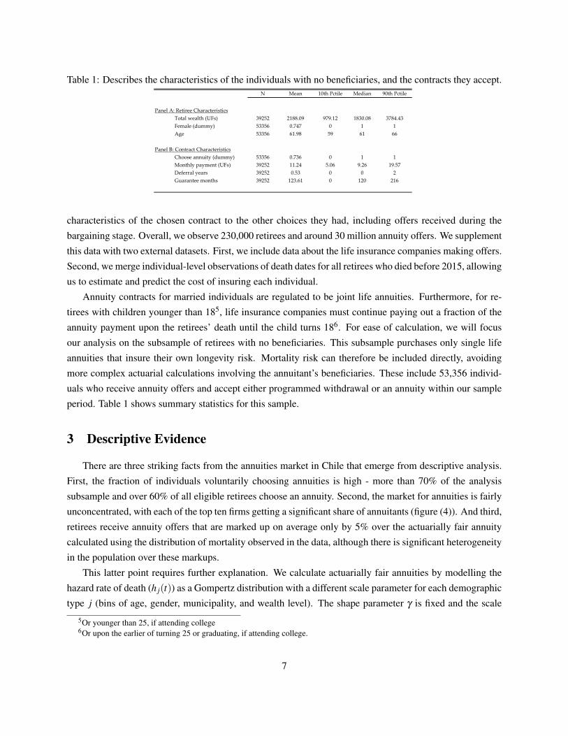
Table 1: Describes the characteristics of the individuals with no beneficiaries, and the contracts they accept.N Mean 10th Pctile Median 90th Pctile

Panel A: Retiree Characteristics

Total wealth (UFs) 39252 2188.09 979.12 1830.08 3784.43

Female (dummy) 53356 0.747 0 1 1

Age 53356 61.98 59 61 66

Panel B: Contract Characteristics

Choose annuity (dummy) 53356 0.736 0 1 1

Monthly payment (UFs) 39252 11.24 5.06 9.26 19.57

Deferral years 39252 0.53 0 0 2

Guarantee months 39252 123.61 0 120 216

characteristics of the chosen contract to the other choices they had, including offers received during the

bargaining stage. Overall, we observe 230,000 retirees and around 30 million annuity offers. We supplement

this data with two external datasets. First, we include data about the life insurance companies making offers.

Second, we merge individual-level observations of death dates for all retirees who died before 2015, allowing

us to estimate and predict the cost of insuring each individual.

Annuity contracts for married individuals are regulated to be joint life annuities. Furthermore, for re-

tirees with children younger than 185, life insurance companies must continue paying out a fraction of the

annuity payment upon the retirees’ death until the child turns 186. For ease of calculation, we will focus

our analysis on the subsample of retirees with no beneficiaries. This subsample purchases only single life

annuities that insure their own longevity risk. Mortality risk can therefore be included directly, avoiding

more complex actuarial calculations involving the annuitant’s beneficiaries. These include 53,356 individ-

uals who receive annuity offers and accept either programmed withdrawal or an annuity within our sample

period. Table 1 shows summary statistics for this sample.

3 Descriptive Evidence

There are three striking facts from the annuities market in Chile that emerge from descriptive analysis.

First, the fraction of individuals voluntarily choosing annuities is high - more than 70% of the analysis

subsample and over 60% of all eligible retirees choose an annuity. Second, the market for annuities is fairly

unconcentrated, with each of the top ten firms getting a significant share of annuitants (figure (4)). And third,

retirees receive annuity offers that are marked up on average only by 5% over the actuarially fair annuity

calculated using the distribution of mortality observed in the data, although there is significant heterogeneity

in the population over these markups.

This latter point requires further explanation. We calculate actuarially fair annuities by modelling the

hazard rate of death (h j(t)) as a Gompertz distribution with a different scale parameter for each demographic

type j (bins of age, gender, municipality, and wealth level). The shape parameter γ is fixed and the scale

5Or younger than 25, if attending college6Or upon the earlier of turning 25 or graduating, if attending college.

7

Figure 4: Contracts accepted by subsample of retirees, where the leftmost bar represents programmed with-drawal and the others refer to annuities sold by the top 10 annuity providers.

050

0010

000

1500

0N

umbe

r of a

nnui

ties

Prog

ram

med

With

draw

alCO

NSO

RCIO

NAC

IONA

L

MET

LIFE

CORP

VID

A

SURA

PRIN

CIPA

L

OHI

OCR

UZ D

EL S

UR

BICE

CHIL

ENA

CONS

OLI

DAD

A

PENT

A

Accepted firm

Accepted Annuities/PW by Firm

parameter is modeled as λ j = ex jβ . The resulting hazard rate is given by:

h j(t) = λ jeγt (1)

Since we observe death before 2015, we can estimate this model directly for our sample. Using the results

of this estimation, we can predict expected mortality probabilities for each individual and calculate the net

present cost of an annuity with a monthly payout zt , discounted at rate r. The predicted survival probabilities

(dependent on age, gender, wealth, and municipality) are denoted as {πit}. The NPV of an annuity can then

be calculated as:

NPV (zi) =T

∑t=0

πitzi

(1+ r)t (2)

Naturally, the value of the annuity payout depends on the total retirement savings the retiree gives the life

insurance company (denoted by wi). We calculate percentage markup over cost (equal to the inverse of the

moneys worth ratio minus one) as:

mi =wi−NPV (zt)

NPV (zt)=

1MWRi

−1 (3)

Figure 5 shows the average markup over the actuarially fair annuity that retirees are offered, by their

wealth percentile, for our no-beneficiary subsample. The pricing shows clear evidence of price discrimina-

tion, with the lowest wealth retirees getting prices that are as high or higher than the US average of 0.1-0.15.

The highest wealth retirees, on the other hand, are offered actuarially fair, or better, annuities. Figure 6

8

Figure 5: Markup over actuarially fair price by wealth percentile, where .1 corresponds to a net presentvalue of the annuity being .9*wealth.

0.1

.2.3

.4Av

g M

arku

p

0 20 40 60 80 100Percentile Wealth

Offered Markups by Wealth

Figure 6: Fraction of retirees choosing annuities over PW by percentile of wealth.

.4.5

.6.7

.8Fr

actio

n An

nuiti

zed

0 20 40 60 80 100Percentile Wealth

Offered Markups by Wealth

9

Table 2: Reports the money’s worth ratio of programmed withdrawal and annuities.

Annuity PW

No Bequest 0.789 0.925

Bequest = 2.5% 0.896 0.955

shows the probability of choosing an annuity differentially by wealth percentile. The probability of taking

an annuity is low for the lowest wealth and highest wealth individuals. The first finding follows from the

pricing evidence: low wealth individuals receive expensive offers, and as a result are more likely to select

into programmed withdrawal. In discussions with industry experts, we’ve learned that it is costlier to service

annuities that are slightly above the minimum pension guarantee, as firms expect that in the future the MPG

will rise above the annuity payment and they will have to start coordinating with the government to transfer

the top-up amount to the annuitant. As a result, fewer firms bid on low wealth annuitants, leading to higher

prices. As for the highest wealth individuals, it is clear that they have a lower valuation for annuities, which

leads to lower annuitization rates despite lower equilibrum prices. However, one cannot pinpoint if this

is due to the role of wealth outside the system, bequest motives, or other unobserved preferences without

estimating preferences for products. We will return to this result when discussing our demand estimates.

A first pass at comparing the value of annuities relative to PW is to repeat the exercise done in prior

literature, which solves for the amount of annuitized (or PW-funding) wealth that provides equal utility to

1 unit of non-annuitized wealth. This amount is the money’s worth ratio (”MWR”). Mitchell et al. (1999)

perform this calculation for US retirees without a bequest motive facing actuarially fair annuities, and found

an MWR of 0.7. Results from MWR calculations in our setting are shown in table 2. We find somewhat

similar results for actuarially fair annuities in Chile - if the retiree has no bequest motives, she would be

willing to give up 21.1% of her wealth to get an actuarially fair annuity. With a bequest motive of 2.5%7,

the MWR is 0.90, so an annuity is worth giving up 10.4% the value of non-annuitized wealth. In both cases,

it is clear that annuities are valuable products. The analogous calculation for PW is enlightening - relative

to no annuitization, a retiree without a bequest motive has a PW MWR of 0.925, meaning they are willing

to pay 7.5% of their wealth to obtain access to PW. With a bequest motive, getting access to PW is worth

4.5% of her wealth. It should not be surprising that PW has an MWR below one, as the minimum pension

guarantee provides some annuitization value. The main takeaway from this exercise, then, is to show that

PW is providing relatively high net value. Retirees choosing annuitization in Chile, therefore, are likely not

doing so because PW is a bad product.

Though the market is functioning remarkably well, many features of the data reflect standard intuitions

about annuity markets worldwide. First, there is significant adverse selection into annuity purchase. To

demonstrate this, we run the standard positive correlation test, introduced by Chiappori and Salanie (2000).

In our implementation of this test, we regress the probability the retiree dies within two years of retirement,

regressed on a dummy for annuity choice. Table 3 shows this baseline correlation in column 1. Columns

740 dollars of bequeathed wealth are equivalent to 1 of own wealth.

10

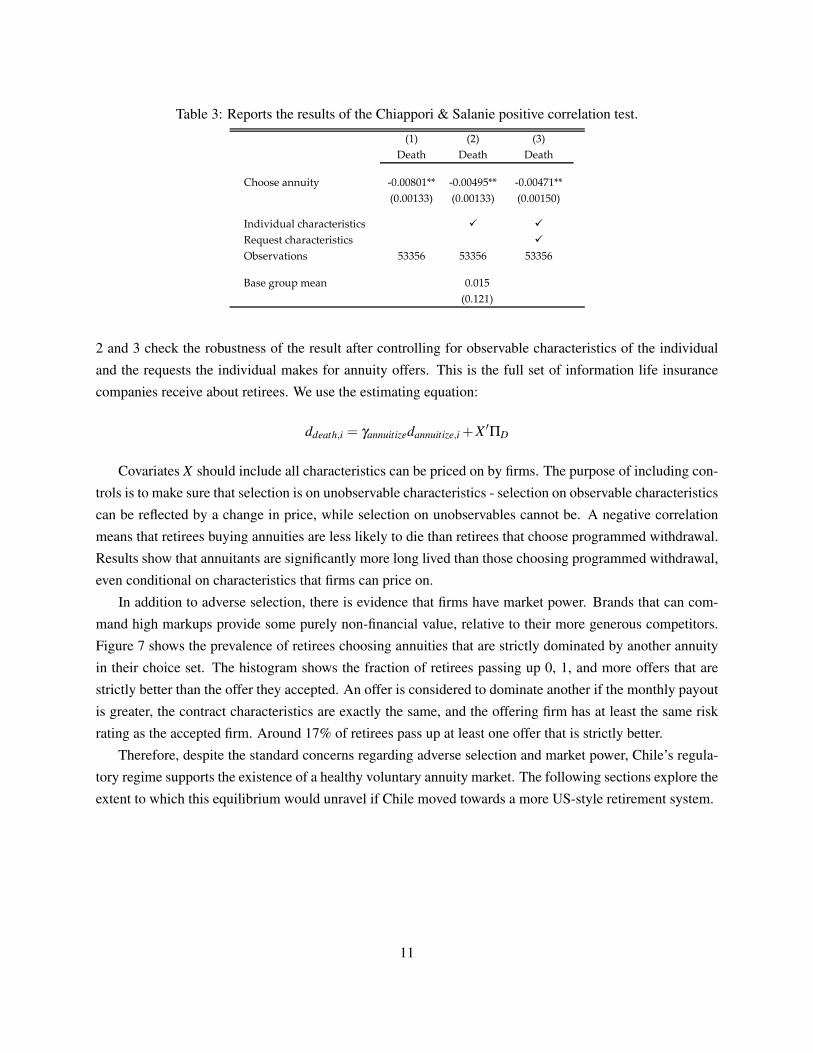
Table 3: Reports the results of the Chiappori & Salanie positive correlation test.

(1) (2) (3)

Death Death Death

Choose annuity -0.00801** -0.00495** -0.00471**

(0.00133) (0.00133) (0.00150)

Individual characteristics ✓ ✓

Request characteristics ✓

Observations 53356 53356 53356

Base group mean 0.015

(0.121)

2 and 3 check the robustness of the result after controlling for observable characteristics of the individual

and the requests the individual makes for annuity offers. This is the full set of information life insurance

companies receive about retirees. We use the estimating equation:

ddeath,i = γannuitizedannuitize,i +X ′ΠD

Covariates X should include all characteristics can be priced on by firms. The purpose of including con-

trols is to make sure that selection is on unobservable characteristics - selection on observable characteristics

can be reflected by a change in price, while selection on unobservables cannot be. A negative correlation

means that retirees buying annuities are less likely to die than retirees that choose programmed withdrawal.

Results show that annuitants are significantly more long lived than those choosing programmed withdrawal,

even conditional on characteristics that firms can price on.

In addition to adverse selection, there is evidence that firms have market power. Brands that can com-

mand high markups provide some purely non-financial value, relative to their more generous competitors.

Figure 7 shows the prevalence of retirees choosing annuities that are strictly dominated by another annuity

in their choice set. The histogram shows the fraction of retirees passing up 0, 1, and more offers that are

strictly better than the offer they accepted. An offer is considered to dominate another if the monthly payout

is greater, the contract characteristics are exactly the same, and the offering firm has at least the same risk

rating as the accepted firm. Around 17% of retirees pass up at least one offer that is strictly better.

Therefore, despite the standard concerns regarding adverse selection and market power, Chile’s regula-

tory regime supports the existence of a healthy voluntary annuity market. The following sections explore the

extent to which this equilibrium would unravel if Chile moved towards a more US-style retirement system.

11

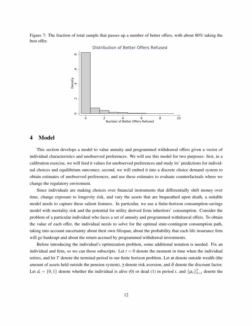
Figure 7: The fraction of total sample that passes up a number of better offers, with about 80% taking thebest offer.

0.2

.4.6

.8D

ensi

ty

0 2 4 6 8 10Number of Better Offers Refused

Distribution of Better Offers Refused

4 Model

This section develops a model to value annuity and programmed withdrawal offers given a vector of

individual characteristics and unobserved preferences. We will use this model for two purposes: first, in a

calibration exercise, we will feed it values for unobserved preferences and study its’ predictions for individ-

ual choices and equilibrium outcomes; second, we will embed it into a discrete choice demand system to

obtain estimates of unobserved preferences, and use these estimates to evaluate counterfactuals where we

change the regulatory enviroment.

Since individuals are making choices over financial instruments that differentially shift money over

time, change exposure to longevity risk, and vary the assets that are bequeathed upon death, a suitable

model needs to capture these salient features. In particular, we use a finite-horizon consumption-savings

model with mortality risk and the potential for utility derived from inheritors’ consumption. Consider the

problem of a particular individual who faces a set of annuity and programmed withdrawal offers. To obtain

the value of each offer, the individual needs to solve for the optimal state-contingent consumption path,

taking into account uncertainty about their own lifespan, about the probability that each life insurance firm

will go bankrupt and about the return accrued by programmed withdrawal investments.

Before introducing the individual’s optimization problem, some additional notation is needed. Fix an

individual and firm, so we can those subscripts. Let t = 0 denote the moment in time when the individual

retires, and let T denote the terminal period in our finite horizon problem. Let ω denote outside wealth (the

amount of assets held outside the pension system), γ denote risk aversion, and δ denote the discount factor.

Let dt = {0,1} denote whether the individual is alive (0) or dead (1) in period t, and {µτ}Tτ=1 denote the

12

vector of mortality probabilities 8. Following Carroll (2011), let ct denote consumption in period t, mt the

level of resources available for consumption in t, at the remaining assets after t ends, and bt+1 the “bank

balance” in t +1.

For the purposes of specifying the optimal consumption-savings problem given an annuity offer, we

also need to define qt , which denotes whether the firm is bankrupt (1) or not (0) in period t, and the vector

of bankruptcy probabilities for the offering firm {ψ j,τ}Tτ=1

9. With these objects, we can write the annuity

payment in period t conditional on dt , qt , the deferral period D and the guarantee period G as zt(dt ,qt ,D,G).

With this notation, and suppressing individual and firm subscripts, we can write the individual’s optimal

consumption problem given an annuity offer as:

maxE0

[T

∑τ=0

δτu(cτ ,dτ)

](4)

s.t.

at = mt − ct ∀t

bt+1 = at ·R∀t

mt+1 = bt+1 + zt+1(dt+1,qt+1,D,G)∀t

at ≥ 0∀t

Where R = 1+ r, and r is the real interest rate10, which we assume is deterministic and fixed over time.

Note that we are imposing a no borrowing constraint: there can be no negative end of period asset holdings.

This assumption greatly simplifies the problem from a computational perspective, and to the best of our

knowledge Chilean financial institutions do not allow individuals to borrow against future annuity or PW

payments.

8Clearly, d0 = 0 and µ0 = 09Naturally q0 = 0 and ψ0 = 0

10Annuity and PW offers in Chile are expressed in UFs, an inflation-adjusted currency, so everything in the model is in realterms.

13

The exogenous variables evolve as follows:

dt+1 =

0 with probability (1−µt+1) if dt = 0

1 with probability µt+1 if dt = 0

1 if dt = 1

(5)

qt+1 =

0 with probability (1−ψt+1) if qt = 0

1 with probability ψt+1 if qt = 0

1 if qt = 1

(6)

zt(dt ,qt ,D,G) =

z if qt = 0 and ((dt = 0 and t ≥ D) or (dt = 1 and D≤ t < G+D))

ρ(z, t) · z if qt = 1 and ((dt = 0 and t ≥ D) or (dt = 1 and D≤ t < G+D))

0 otherwise

(7)

m0 = ω, d0 = 0, q0 = 0 (8)

Where ρ(z, t) is the annuity payment when the firm goes bankrupt:

ρ(z, t) =

MPGt if z≤MPGt

MPGt +min((z−MPG)∗0.75,45) if z > MPG(9)

and MPG is the minimum pension guarantee. For the purposes of this model, we will assume that

the MPG is fixed over time. Assume that the utility derived from consumption when alive is given by the

following CRRA utility function:

u(ct ,dt = 0) =c1−γ

t

1− γ(10)

whereas if the individual dies at the beginning of period t, her terminal utility at t is given by evaluating the

CRRA at the expected value of remaining wealth11:

u(dt = 1) = β ·(mt +E[∑G

τ=t+1 δ t−τzτ(1,qτ ,D,G)])1−γ

1− γ(11)

and is equal to zero thereafter.

To obtain the value of an annuity offer, which is the present discounted value of the expected utility of the

optimal state-contingent consumption path, we solve this problem by backward induction. At the terminal

11This assumption implies that individuals are not risk averse about the remaining uncertainty after death. If they were, we’dneed to calculate expected utility instead of the utility of the expectation. From a practical perspective, this is unlikely to mattermuch, as the only case where remaining wealth is stochastic is for annuity offers with a guarantee period from firms who have notgone bankrupt, as wealth left to inheritors in this case is still subject to bankruptcy risk. Since bankruptcy risk is small, and mostdeaths will occur after the guarantee period expires, we are comfortable making this assumption.

14

period, the problem is simple and has an analytic solution, but for periods earlier than T it must be solved

numerically. We use the Endogenous Gridpoint Method (EGM) (Carroll (2006)) to solve this problem,

obtaining V A(0,0;π), the present discounted value of the expected utility of consumption obtained from

following the optimal state-contingent policy path given an annuity offer and the vector π of parameters12.

See Appendix B for the full derivation of the Euler equations and the computational details of the numerical

solution.

Valuing a programmed withdrawal (PW) offer requires solving a related, but slightly different, problem.

In this setting there is no deferral or guarantee period, or bankruptcy risk for the asset. Furthermore, in-

heritors automatically receive all remaining balances as a bequest upon death. All of these factors simplify

the problem relative to the annuity problem. However, a significant complication arises: PW payouts are a

function of the amount of money left in the PW account, which varies stochastically with market returns.

As a result, the PW stock in period t, PWt , becomes an additional state variable. Taking these differences

into account, the individual’s PW optimization problem, which gives us the value of accepting a PW offer

from firm a, is:

maxE0

[T

∑τ=0

δτu(ct ,dt)

](12)

s.t.

at = mt − ct ∀t

bt+1 = at ·Rt+1∀t

mt+1 = bt+1 + zt+1(PWt+1,dt+1, f )∀t

at ≥ 0∀t

where zt(PWt ,dt , f ) denotes the programmed withdrawal payout in period t conditional on pension balance

PWt , death status, and f , the commission rate charged by the firm. The death state and initial conditions are

as before (Equation 5), and the remaining exogenous variables evolve as follows:

zt(PWt ,dt ,a) =

max[zt(PWt) · (1− τa),MPG] if dt = 0

0 if dt = 1(13)

PWt+1 = (PWt − zt(PWt)) ·RPWt (14)

The PW payout function zt(PWt) is described in detail in Appendix A. All PFAs are governed by the same

PW function, and conditional on the PW balance, will pay out the same amount up before the commission

f . As a result, if PFAs provided the same returns over time, the amount of money that is withdrawn every

year from the PW account would be the same across PFAs, and only how that money is distributed between

the retiree and the PFA would vary across companies. We will assume that in fact PFAs provide the same

12Outside wealth ω , bequest motive β , mortality probabilities {µ}Tt=1, risk aversion γ , and bankruptcy probabilities {ψ}T

t=1

15

returns on PW investments, as this simplifies the problem and is not far from reality, where PFA returns

vary slightly for the safe investment portfolios where PW balances are invested 13. Let RPWt be the return

to programmed withdrawal investments. We assume lnRPWt ∼ N(ln(R+ r)−σ2

PW/2,σ2PW ), with r denoting

the equity premium of PW over the market interest rate R. Finally, MPG is the minimum pension guarantee.

Every individual who takes PW is guaranteed a payout of at least MPG, and the difference between zt(PWt)

and MPG (when zt(PWt) < MPG) is funded by the government. Finally, utility derived from consumption

is as before, while upon death utility is:

u(dt = 1) = β · (mt +PWt)1−γ

1− γ(15)

As for annuities, we solve this problem numerically by backwards induction using EGM, and obtain V PW (0,PW0;π),

the present discounted value of the expected utility of consumption obtained from following the optimal

state-contingent policy path given an initial PW balance of PW0 and the vector π of parameters. See Ap-

pendix B for the full derivation of the Euler equations and the computational details of the numerical solu-

tion.

5 Calibration

In this section, we calibrate the previous life cycle model and calculate the value of an annuity relative to

programmed withdrawal for different mortality beliefs. With a given distribution of mortality expectations,

we map these utilities to a model of market equilibrium by calculating demand for annuities and average

cost of supplying annuities. We then change the alternative to annuitization, following Mitchell et al. (1999),

to mimic US-style social security, and study how the market equilibrium changes.

We model heterogeneity in mortality risk as shifts over the mortality tables used by the Chilean pension

authorities14. More precisely, given a retiree’s age, these tables give us a mortality probability vector. We

introduce heterogeneity as shifts in the individuals’ age, so that a 65 year old retiree with a x year mortality

shifter has the mortality probability vector of a 65+ x year old. This allows us to introduce unobserved

heterogeneity in mortality risk in a parsimonious way, at the cost of assuming that all shifts in mortality

preserve the shape of the regulatory agencies’ tables15.

For ease of exposition, all other parameters in the model are fixed in this section. The representative

retiree is drawn from the data - a 60 year old female, retiring in 2007 with relatively high wealth. Parameters

of the utility function are taken from previous literature when possible. The risk aversion parameter is

3, interest rate is 3.18% (yearly), the standard deviation of the mortality shifter is 7, the bequest motive

13Illanes (2017) documents this in detail14Superintendencia de AFP and Superintendencia de Valores y Seguros15These tables are specifically designed to capture the mortality expectations of the annuitant population.

16

Figure 8: Comparison of utility levels from annuity purchase vs programmed withdrawal, given privateinformation about life expectancy as shown on x axis.

parameter is 10, and the fraction of the retiree’s total wealth annuitized is 20%16. The utility obtained from

the retiree annuitizing is calculated based on the choice of an annuity with no deferral or guarantee period.

The alternative to annuitization is programmed withdrawal, which follows the standardized schedule set

by the government. That is, we are abstracting away from heterogeneity in preferences for contracts and

preferences for firms. We will return to these issues below, in the context of demand estimation.

Figure 8 shows the utility levels obtained from retirees choosing an annuity vs. programmed withdrawal.

The x axis corresponds to different values of life expectancy after retirement, while the y axis is in utility

space. Retirees with a very low mortality shifter, meaning their probability of death is significantly higher

than their calendar age, would prefer to take programmed withdrawal over an annuity. The benefit of pro-

grammed withdrawal is that retirees get larger payouts in the first few years after retirement than they would

receive from an annuity, and the remainder of the savings is passed on to the retirees’ beneficiaries. The

value of programmed withdrawal is comparable to that of an annuity at all mortality shifters, but of course

as life expectancy increases the annnuity dominates.

Given the utility levels at each mortality shifter, demand can be derived by imposing a distribution over

mortality shifters. Demand is calculated as the monthly payout from an annuity that makes the marginal

consumer indifferent between taking an annuity and programmed withdrawal. We call this value the ”indif-

ference annuity”. The result is plotted in figure 9. The x axis shows the fraction of the population purchasing

an annuity, and the y axis shows the value of the indifference annuity. The green line, labelled “Marginal

Indifference”, denotes the demand function, while the solid red line, labelled ”Fair Annuity”, is average cost.

Note that demand is upward sloping on these axes, since a higher pension payout is equivalent to a lower

16Wealth in the pension system is 2200 UFs, and outside wealth is 8800 UFs

17

Figure 9: Demand for annuities as a function of markup over actuarially fair annuity for mean individualrelative to average cost to firm of insuring that population implied equilibrium annuitization rate of 99%assuming zero load, with 97% annuitization with 15% load.

price for a standard good. Therefore, the first individuals to annuitize are those with the lowest indifference

annuities, as they would be willing to accept the least generous offers (highest prices). And as the fraction

of the population that annuitizes increases, the indifference annuity increases as well: marginal annuitants

value annuities less and less, so they need higher payouts (lower prices). From the same parameters, we can

also calculate average cost given an annuitant population as the pension payout that lets the firm break even

(hence “fair annuity”). Since the only source of heterogeneity in this calibration is mortality risk, individuals

with the highest valuation for annuities are also the longest-lived, and therefore the costliest. As a result,

the annuity payout that lets the firm break even also increases as more individuals annuitize, as the marginal

annuitant is always shorter lived than the inframarginal annuitants.

The intersection of the average cost curve and demand describes the market equilibrium under perfect

competition. At the equilibrium in figure 9, annuitization rate is about 99%. As this is under perfect

competition, there is no load over the average cost for the annuitized fraction of the population. The dotted

lines show the effect of adding a load of 5 or 10%, which results in a lower pension payout to retirees. The

load may be due to administrative costs or to market power that allows life insurance firms to make positive

profits. Figure 9 shows that a load of 5 or 10% decreases the annuitization rate very little, with the new

equilibrium annuitization rate being about 90%. This is due to demand being locally inelastic: near full

annuitization, the marginal consumers have a very low valuation for annuities and therefore must be offered

very high annuity payments. The steepness of the demand curve around full annuitization implies that

adding a load doesn’t shift the fraction annuitized in an economically significant amount. In this calibration,

the high annuitization equilibrium in Chile is very stable in the face of potential supply side changes.

To contextualize these calibration results, we construct a counterfactual equilibrium in the presence of

18

Figure 10: Comparison of utility levels from annuity purchase vs US-style social security, given privateinformation about life expectancy as shown on x axis.

US-style regulations. Following Mitchell et al. (1999), we model Social Security as an actuarially fair

annuity provided for half of the individual’s pension savings, while the other half is unconstrained and may

be annuitized in the private market. Figure 10 compares the utility obtained from annuitizing the remaining

wealth (”Annuity”) with the utility obtained from keeping the remaining wealth liquid. Figure 11 presents

the results of the same supply-and-demand analysis as before. Average cost (per-dollar annuitized) remains

the same, as the mortality distribution has not changed. Note, however, that the existence of Social Security

significantly changes the demand function, as now retirees value annuities less and the demand function is

shallower. Since 50% of pension wealth is already annuitized, exposure to longevity risk is significantly

lower, lowering willingness to pay and smoothing out its differences across retirees. Despite these changes,

in the no-load scenario we still see almost full annuitization17, as in the Chilean equilibrium.

Once a load is added, though, the US-style equilibrium changes very significantly. In fact, a 10% load

causes the entire market to unravel. This is due to the combined effects of the shift up in the indifference

annuity, as well as the flattening of the demand function. Therefore, in the US setting adverse selection

has a stronger effect on demand for annuities, since Social Security provides a more comparable product

to full annuitization than the programmed withdrawal outside option. Then, the regulatory environment of

US-style Social Security causes the annuity market equilibrium to be much more sensitive to loads. Any

market power or administrative cost has the potential to completely unravel the equilibrium.

The calibration shows that Chile’s unique exception to the annuity puzzle could be driven in part by the

design of programmed withdrawal, relative to US-style Social Security, as well as potentially lower loads.

17While demand and average cost intersect twice, only the higher intersection is an equilibrium because average cost mustintersect demand from below in order for the firm to break even.

19

Figure 11: Demand for annuities as a function of markup over actuarially fair annuity for mean individualrelative to average cost to firm of insuring that population implied equilibrium annuitization rate of 99%assuming zero load, with 0% annuitization with 15% load.

Of course, these examples are for a particular combination of parameters, so we need to estimate demand

to determine whether the arguments borne out in these calibrations are fleshed out in the data. Furthermore,

with a demand system we can address the welfare implications of both retirement systems.

In addition, we have shown that both demand and average cost are nonlinear, which has a significant

impact on equilibrium outcomes. This implies that in order to estimate the differential level of selection

in Chile and its contribution to the high annuitization rate, we cannot rely on linear approximations to the

demand and cost curves. That approach, which is successful in calculating welfare and counterfactuals in

contexts like health insurance (Einav et al. (2010)), would not capture the relatively sudden unraveling of the

US market relative to the Chilean market. In the following sections, we proceed to identify the underlying

distribution of private information that drives both demand and cost curves.

6 Demand Estimation

In this section, we embed the numerical solutions to the model introduced in Section 4 into a demand

estimation framework to recover distributions of unobserved preferences. We will then use these estimates

in Section 7 to study the impact of different features of the Chilean retirement exchange on equilibrium

outcomes. This section is divided into three parts. The first present the demand estimation model, the

second discusses implementation details, and the third presents the intuition for identification.

20

6.1 Framework

Denote the value of an annuity offer o that firm j makes to individual i by V Aio j(θ), and the value of

taking programmed withdrawal from PFA j as V PWi j . In appendix B, we derived how to calculate these val-

ues as a function of the characteristics of the contract, individual observables such as age and gender, and

individual unobservables such as initial wealth, risk aversion, bequest motive and mortality and bankruptcy

probabilities. However, the descriptive evidence presented in Section 3 makes it clear that these values are

not sufficient to explain choices in this setting, as a significant fraction of the population are accepting dom-

inated offers. That is, there must be non-financial preferences for contracts affecting individuals’ valuations.

To introduce such differentiation, we model individual i’s utility from an annuity offer o from firm j and

from taking PW from firm a as:

UAio j =V A

io j +ξ j +ξo +ξo j + εio j (16)

UPWia =V PW

ia +ξa + εia (17)

We assume that ε is iid and follows an Extreme Value Type I distribution. These assumptions imply that

the utility of an annuity offer is equal to the expected utility derived from the solution to the consumption-

savings problem plus four terms that are unobserved to the econometrician: a firm preference ξ j, a contract

preference ξo, a firm-contract preference ξo j, and the logit error. Similarly, the utility of a PW offer is equal

to the expected utility derived from the solution to the consumption-savings problem under that contract plus

an unobserved PFA preference ξa and a logit error. We allow for the possibility that the ξ ’s are observed by

firms when making offers, so that they can be correlated with price. This creates the standard endogeneity

problem in demand estimation, which we will tackle through an exclusion restriction.

To introduce our demand estimation framework, it is important to recap what enters into the value

of an annuity offer and a PW offer, as in Section 4 we conditioned on an individual and an offer and

suppressed notation that denoted heterogeneity. First, age and gender are individual observables that affect

the utility calculation, as individuals retire at different ages and there are significant mortality differences

across genders. Second, there is a series of product characteristics that enter the problem: for annuity offers,

the payment amount, deferral and guarantee periods, and payments upon bankruptcy ρo j; for PW offers, the

fee. We will combine these two sets of observables (and a constant) into a matrix Xio j. Third, there is a series

of unobservables that enter the problem: risk aversion γi, outside wealth ωi, bequest motive βi, mortality

probability vector µi, and bankruptcy probability vector ψi. We will assume that these unobservables are

jointly distributed according to a distribution F , and denote an individual’s draw from F by πi. Then:

UAio j =V A(Xio j,πi)+ξ j +ξo +ξo j + εio j (18)

UPWia =V PW (Xia,πi)+ξa + εia (19)

21

We can then write the probability that individual i chooses annuity offer o from firm j as:

sio j(Xi,π,ξ ) =∫ exp(V A(Xio j,π)+ξ j +ξo +ξo j)

∑o′, j′ exp(V A(Xio′ j′ ,π)+ξ ′j +ξ ′o +ξo′ j′)+∑a exp(V PW (ia,π)+ξa)dF(π) (20)

while the probability that they pick programmed withdrawal from PFA a is:

sia(Xi,π,ξ ) =∫ exp(V (Xia,π)+ξa)

∑o′, j′ exp(V A(Xio′ j′ ,π)+ξ ′j +ξ ′o +ξo′ j′)+∑a exp(V PW (Xia,π)+ξa)dF(π) (21)

If every individual received the same set of annuity offers from the same set of firms, we could average overindividuals to obtain market shares. However, not every life insurance company bids on every individual,and not every individual requests the same set of contracts. We assume that the set of requested contractsand the set of received offers is exogenous, and denote the set of received offers by Bi. Over the full spaceof offers B, we have that sio j = 0 if o, j /∈Bi, and that:

sio j(Xi,π,ξ ) = 1 [o, j ∈Bi] ·∫ exp(V A(Xio j,π)+ξ j +ξo +ξo j)

∑o′, j′∈Bi exp(V A(Xio′ j′ ,π)+ξ ′j +ξ ′o +ξo′ j′)+ξ ′j)+∑a exp(V PW (Xia,π)+ξa)dF(π)

sia(Xi,π,ξ ) =∫ exp(V (Xia,π)+ξa)

∑o′, j′ exp(V A(Xio′ j′ ,π)+ξ ′j +ξ ′o +ξo′ j′)+∑a exp(V PW (Xia,π)+ξa)dF(π) (22)

Averaging across individuals yields aggregate shares:

so j(X ,π,ξ ) = N−1N

∑i=1

sio j(Xi,π,ξ ) (23)

sa(X ,π,ξ ) = N−1N

∑i=1

sia(Xi,π,ξ ) (24)

With this structure and our individual choice and demographic data, one could estimate this model as a

standard logit demand system with random coefficients and micro moments, as in Petrin (2002) or Berry

et al. (2004). One challenge, however, is that one would have to re-solve the optimal consumption problem

for every individual-offer-firm combination for every guess of the parameters governing the distribution F .

This is extremely expensive from a computational perspective. Instead, we follow the intuition of Ackerberg

(2009) and pre-solve the optimal consumption-savings problem for a grid of π , and then estimate the weights

over that grid that minimize a GMM objective function. The resulting estimator is a semi-parametric demand

system that is very similar to Fox et al. (2011) and Nevo et al. (2016). Our methodological contribution is

that we embed this procedure into the micro-BLP framework, which allows us to incorporate exclusion

restrictions between instruments Z and the unobserved firm-offer component of utility. This allows us

to retain the structure from micro-BLP, but with a non-parametric distribution for the vector of random

coefficients.More precisely, we solve the optimal consumption-savings problem for every individual-offer over a

grid in the space of π . Let πr denote one element of this grid, and φr the probability mass at that point. Then

22

we can write the probability that an individual chooses an offer as:

sio j(Xi,φ ,ξ ) = 1 [o, j ∈Bi] ·R

∑r=1

exp(V A(Xio j,πr)+ξ j +ξo +ξo j)

∑o′, j′∈Bi exp(V A(Xio′ j′ ,πr)+ξ ′j +ξ ′o +ξo′ j′)+ξ ′j)+∑a exp(V PW (Xia,πr)+ξa)φr

sia(Xi,φ ,ξ ) =R

∑r=1

exp(V PW (Xia,πr)+ξa)

∑o′, j′ exp(V A(Xio′ j′ ,πr)+ξ ′j +ξ ′o +ξo′ j′)+∑a exp(V PW (Xia,πr)+ξa)φr (25)

Which allows us to write aggregate shares as:

so j(X ,φ ,ξ ) = N−1N

∑i=1

sio j(Xi,φ ,ξ )

sa(X ,φ ,ξ ) = N−1N

∑i=1

sia(Xi,φ ,ξ ) (26)

We can then write our demand estimation problem as:

minφ ,ξ

g(X ,Z,D,φ ,ξ )′V−1g(X ,Z,D,φ ,ξ ) (27)

subject to:

so j(X ,φ ,ξ ) = so j ∀o, j (28)

sa(X ,φ ,ξ ) = sa∀a (29)

0≤ φr ≤ 1∀r (30)R

∑r=1

φr = 1 (31)

h(φ) = 0 (32)

where g(X ,Z,D,φ ,ξ ) consists of the following moments:

E[ξo j ·Zo j] = 0 (33)

E[ξa ·Za] = 0 (34)

E[Xhio j ·Dk

i · [1[i chooses o,j]− sio j(Xi,W,π,ξ )]] = 0∀o, j,h,k (35)

E[Xhia ·Dk

i · [1[i chooses a]− sia(Xi,W,π,ξ )]] = 0∀a,h,k (36)

where k denotes a particular variable in a matrix D of individual observables, and h denotes a particular

variable in the matrix X . Equations 33, 34, 28 and 29 are the baseline components of a random coefficients

demand system estimated a la Berry et al. (1995): the set of exclusion restrictions between instruments and

the unobservables and the Berry (1994) inverses. Rather than writing the problem as a nested fixed point,

we’ve written it as an MPEC following Dube et al. (2012), but from a theoretical perspective that difference

is immaterial. Equations 35 and 36 are the micro-moments (Petrin (2002), Berry et al. (2004)), which aim to

23

match the observed covariance between a product’s characteristics and the demographics of the population

that chooses it with the covariance that is predicted by the model. Finally, equations 30,31, and 32 are

restrictions on the distribution of the unobservables. The first two equations are the standard support and

adding-up restrictions, while the third denotes a set of outside restrictions. For example, one could restrict

the marginal distribution of outside wealth to match assets from a survey, or the marginal distribution of

mortality probabilities to match observed mortality.

In order to determine the empirical importance of including non-financial utility components into equa-

tion 16, we will compare the results obtained from the previous model with the results obtained from a direct

application of Fox et al. (2011). In our context, this boils down to specifying utility as:

UAio j =V A

io j + εio j (37)

UPWia =V PW

ia + εia

For every individual-type, we calculate predicted choice probabilities sio jr, and then estimate the weights on

the distribution of types using constrained OLS:

minφ

∑i,o, j

(yio j−∑r

sio jrφr)2 (38)

s.t.

φr ≥ 0∀r

∑r

φr = 1

The key difference between this model and our specification is the lack of non-financial utility terms that

can be priced on. In this model, consumers make purely financial choices up to the logit error, and so price

endogeneity is assumed away. Therefore, the acceptance of dominated offers can only be rationalized by the

logit error. In the following section we present the results from both models and discuss the implications of

assuming away endogeneity of offers.

6.2 Implementation

The goal of the estimation procedure is to recover the joint distribution of unobserved preferences with-

out specifying restrictive functional form assumptions. The combination of the Berry inverse and the ex-

clusion restrictions with respect to the firm-offer unobservable allow us to deal with endogeneity concerns,

while the micro-moments and the outside restrictions discipline the distribution of unobserved preferences.

Of course, up to this moment we haven’t specified what the instruments or the micro-moments actually

are, so we return to this discussion below. Up to now, our goal is simply to introduce the general estima-

tion framework, and to note that this is a way to bring exclusion restrictions and micro-moments into the

semiparametric estimation framework of Fox et al. (2011). We will now discuss the details of the current

24

implementation.

First, we need to pick a grid over the space of π . Recall that F(π) is the joint distribution of risk aversion

γ , initial wealth ω , bequest motive β , mortality probability vector µ and bankruptcy probability vector ψ .

Clearly, we need to impose additional restrictions on these objects, or creating a grid over this space will be

computationally infeasible (µ alone is a T ×1 object). First, we will model the mortality probability vector

µ as the mortality vector from the tables used by the Chilean pension authorities18, plus an unobserved

component that shifts individuals up or down this vector. For example, an individual who retires at 60

with a mortality shifter value of 2 solves the optimal consumption-savings problem for each contract using

the mortality vector of a 62 year old in the Chilean tables. This allows the model to continue to feature

adverse selection into contracts, as individuals with low (high) mortality shifter draws are unobservably

younger (older) than their age, without having to separately identify whether this selection comes from a

higher death probability in year x or x+ 1. Second, we assume away bankruptcy risk. While bankruptcy

risk is theoretically relevant, there has only been one bankruptcy since the system’s inception, and even in

that case the company’s annuitants continued to receive their full annuity payments for 124 months and the

governmental guarantee amount after 19. As a result, it is difficult to find variation in the data that would

identify a distribution of bankruptcy risk, particularly after controlling for a firm fixed effect.

This shrinks the dimensionality of the grid to 4: risk aversion, initial wealth, bequest motive, and mor-

tality shifter. We will also restrict the risk aversion parameter to be equal to 3, following the previous

literature20. Now we have a 3 dimensional grid. We solve the optimal consumption-savings problem for

every individual-firm-annuity offer, imposing δ = 0.95, and R = 1.03. For programmed withdrawal, since

PW fees are almost identical across companies and we are not interested in modelling substitution across

PFAs, we solve the optimal consumption-savings problem for one PW offer, assuming the fee is the median

fee. Furthermore, we assume that the PW problem is non-stochastic (σPW = 0)21, and set the mean PW

return to its empirical counterpart.

For every individual-annuity/PW contract, we pre-solve the consumption-savings problem for 25 equally-

spaced grid points in each dimension of unobserved preference. This implies solving each problem for a

grid of 15,625 points. For bequest motive β , the support of the grid is [0,52]. The lower bound implies

individuals do not value their heirs’ consumption, while in calibrations we found that for levels of β above

the upper bound individuals would sacrifice themselves to save money for their heirs. For outside wealth (in

UFs), the support of the grid is [0,30.000]22. This upper bound corresponds to $1.225.650 USD.23. Finally,

the support of the mortality shifter grid is [−12,12]. This implies that the healthiest (sickest) person has the

18Superintendencia de AFP and Superintendencia de Valores y Seguros19The goverment guarantee after a bankruptcy is equal to the minimum pension guarantee plus 75% of the difference between this

guarantee and the monthly annuity value, up to a cap of 45 UFs. In December 12, 2017, a UF was worth 40.85 USD. For more detailson the bankruptcy process, see (in Spanish) http://www.economiaynegocios.cl/noticias/noticias.asp?id=35722

20This is temporary. Our short-term goal is to add this dimension to the grid.21Again, this is an assumption that we are planning on relaxing, although in calibration exercises it doesn’t affect the value of

taking PW significantly.22To be precise, the lower bound is 1e−10, as a value of zero generated numerical issues.23As of December 12, 2017

25

mortality probabilities of a person 12 years younger (older). We think that these values span the support

of the distribution of unobservables, allowing for a flexible parameterization of demand. We return to this

discussion in the Results section.

Having discussed how to obtain the value function for every individual-offer-grid point, we now turn to a

discussion of the remaining details of the demand estimation procedure. First, in the previous exposition we

have already implicitly imposed the standard scale normalization that σε = 1. For a location normalization

we set the utility of the now lone programmed withdrawal contract to zero and difference out the value

of PW from the value of every annuity offer24. Second, to deal with endogeneity of the offer amount

we need an instrument that varies at the firm-contract level, shifting the value of an annuity offer while

being independent of the firm-contract unobservable. We use the interaction between the PDV of expected

payouts of a $1 annuity, calculated using the regulatory mortality tables, and the risk rating of a firm as such

an instrument. This PDV expresses the cost in a no-selection world of each annuity contract, and varies

across contract types due to the differential exposure to mortality risk induced by the contract terms. The

interaction with firm risk rating is meant to capture the differential costs firms with different capital costs

face even if they offer the same annuity. We think of this instrument as having a fairly straightforward

mapping to cost shifters in other settings where differentiated products demand systems are estimated. One

source of concern is that risk rating could be correlated with the firm-contract unobservable. However, for

this to introduce bias there would need to be correlation between these variables net of firm and contract

fixed effects, which we do not think is likely. Since the Chilean mortality tables change twice during our

sample period25, we divide the sample into three periods and treat each period as a separate market. This

also allows us to leverage the time variation of the instrument. Implicitly, this implies assuming no selection

into retirement induced by the change in tables. Figures C and C in appendix C presents plots of the

number of retirements over time for a window around the table changes. The fact that there is no bunching

around these cutoffs relieves our concerns about this assumption. Third, the product characteristics that

enter into the micro moments are a constant, a dummy for whether the offer has a free disposal amount,

and the number of guaranteed years and deferral years of the offer. The demographics that enter into the

micro moments are the age and gender of the individual, a dummy for whether they die within 2 years

after retirement, dummies for retirement year, and the amount of money they saved in the pension system

during their lifetime (”inside wealth”). Finally, the additional restrictions on the distribution of unobserved

preferences (h(θ)) come from the 2007 and 2011 waves of Chilean Central Bank’s ”Encuesta Financiera de

Hogares”, which has information on pension account balances and assets outside the pension system. We

use this dataset to calculate the distribution of outside wealth26 conditional on bins of inside wealth27. We

then allow the distribution of outside wealth to vary across quartiles of inside wealth, and impose that for

every bin of inside wealth the distribution of outside wealth matches the distribution in the data.

24Formally, Uia = 0 and Uio j =V A(Xio j,πi)−V PW (Xia,πi)+ξ j +ξo +ξo j + εio j25On 01/31/2005 and 06/30/201026Defined as net asset position27Each bin is a quartile of the pension savings distribution

26

6.3 Intuition for Identification

What is the role that these restrictions play in identifying the demand system? Following the intuition

in Kasahara and Shimotsu (2009), note that given a vector of ξ ’s one can calculate choice probabilities for

every unobservable type. Let S(ξ ) denote the matrix containing these choice probabilities, where columns

are types and rows are individual-products. Since S(ξ )φ = S, the distribution of unobserved preferences,

conditional on ξ , is identified if the matrix S(ξ )′S(ξ ) is invertible. Loosely speaking, this requires that types

have sufficiently different preferences for across contracts. The features of our setting make this likely, as

the financial value of an annuity contract is greatly dependent on the match between the contracts’ terms and

the preferences of the annuitant. For example, as the number of guarantee periods increases, annuity payouts

always decrease. This implies that individuals with no bequest motive will always prefer contracts without

guarantee periods, while as bequest motive increases retirees will value contracts with longer guarantee

periods more.

However, this argument does not pin down ξ , and without it there are many combinations of S(ξ ) and φ

that rationalize choices. To pin down a specific combination of ξ and φ , we bring in the exclusion restrictions

and the micro moments. The exclusion restrictions allow for variations in offer generosity that are orthogonal

to unobserved preference for firm-contracts. If given values of X every individual were identical (had the

same types) then these shifts in price would induce share-based substitution across products. This happens

because in a world with homogenous unobserved preferences given X , our system devolves into a simple

logit. If, however, shifts in offer generosity induce substitution towards products with similar characteristics,

the distribution of unobserved heterogeneity cannot be homogenous and must have greater mass in the

regions where the products for whom we see closer substitution are actually closer substitutes. To fix ideas,

denote a (D,G) contract as an annuity offer with D deferral years and G guarantee years. If after a decrease

in the offer generosity of the (0,0) contract we observe that most consumers substitute towards the (0,10)

contract, preferences must be such that these two contracts are close substitutes. For that to be the case,

some mass of individuals must have a positive bequest motive and a non-trivial probability of dying before

10 years, as otherwise the guarantee years are worthless. If, on the other hand, the closer substitute is the

(5,0) contract, then there must be a mass of consumers who have the liquidity to ride out five years without

annuity payments and who expect to live long enough to reap the benefits of the greater annnuity payment

induced by deferral.

The micro moments further discipline the distribution of unobserved preferences. Since X includes a

constant term, the first set of micro moments simply imposes that for every-contract firm the mean value

of every demographic variable observed in the data matches the mean value predicted by the model. So,

for example, if the mean inside wealth of individuals who choose a (0,10) contract is higher than the mean

inside wealth of individuals who choose the (0,0) contract, it must be the case that the distribution of the

unobservables for individuals with higher inside wealth must have greater mass in the region where the

contract with 10 guaranteed years is optimal. That is, these individuals should have a higher bequest motive

and higher mortality expectations. Furthermore, if after an exogenous decrease in the offer generosity of

27

the (0,0) contract we see that the inside wealth of individuals who take a (0,0) contract increases while

the inside wealth of individuals who take a (0,10) contract decreases, then low inside wealth individuals

who used to take a (0,0) contract are moving to the (0,10) contract. Therefore, these individuals must

find these two contracts to be closer substitutes than high inside wealth individuals, either because they

have higher bequest motives, higher mortality probabilities, or both. The other demographic variables that

enter into the micro moments are age, gender, retirement year and death by two years after retirement.

Age and gender shift the problem by changing the horizon of the optimal consumption problem and the

relevant mortality probabilities28. While, of course, offers also change across these groups, exogenous

shifts in offer generosity affect them differently, and so further discipline the distribution of unobserved

preferences. Retirement year mechanically shifts the generosity of programmed withdrawal, as the payout

function adjusts the mortality tables in a predetermined way every year. Assuming individuals do not select

into retirement based on these changes, imposing that predicted retirement year matches observed retirement

year helps identify substitution to the outside option. Since programmed withdrawal payouts are more front-

loaded than annuities, and remaining balances are inheritable, this also helps identify the joint distribution of

bequest motive and outside wealth. Finally, death by dates allow us to identify the distribution of mortality

beliefs and its correlation to the remaining unobservables. If higher mortality individuals select into contracts

with more guaranteed years, they must also have a bequest motive. If they select into contracts with more

deferral years, they must have greater outside wealth than the rest of the population, such that despite their

greater mortality probabilities they find it optimal to defer.

Note, however, that X does not only include a constant, but also includes product characteristics. As a

result, there is a second set of micro moments that imposes that the model covariance between the product

characteristics of chosen products and the demographics of those who choose them matches the observed

covariance. To gain intuition on these moments, consider the case where every point on the grid of unob-

servables is equiprobable. If under this distribution the covariance of, for example, the number of guaranteed

years and death by two years is lower than what is observed in the data, then mass must be shifted so that

there is more sorting between mortality and preference for guarantee periods. Since the latter is correlated

with having a bequest motive and with having higher mortality expectations, more mass will be placed in

the high mortality-high bequest and low mortality-low bequest portion of the grid, and less placed in the

high mortality-low bequest and low mortality-high bequest space. The last set of moments is the outside re-

strictions with respect to outside wealth. Since we know each individual’s inside wealth and the distribution

of outside wealth conditional on inside wealth, we can impose that the model’s preference estimates satisfy

this conditional distribution and further pin down the distribution of outside wealth.

28Most women in Chile retire at 60, while most men retire at 65.

28

Figure 12: Demand Estimates

7 Results and Counterfactuals

In this draft we present preliminary demand estimates based on the application of Fox et al. (2011) to our

setting (equations 37 and 38). Results from our proposed estimator are pending. These preliminary estimates

are based on a smaller grid over the space of unobservables, with the following values: outside wealth =

1,000, 6,750, 12,500, 18,250 and 24000 UFs; bequest motive = 0, 25, 50, 75, and 100; and mortality shifter

= -16, -8 , 0 , 6 and 16. We allow for different distributions of unobservables across quartiles of pension

wealth. Table 4 presents the results of this exercise. Since there are 500 types in the model, we only report

types with estimated weights above 1%.

Across all pension savings quartiles, most of the mass is located at the corner of the support with outside

wealth 24,000 UFs (980,400 USD), mortality shifter 16, and bequest motive 100. This implies that most

retirees have high bequest motives, low mortality expectations, and a sizeable amount of outside wealth.

However, there is also a significant amount of heterogeneity in the population. For example, in the first

quartile of inside wealth 30.45% of retirees have outside wealth of 1,000 UFs (40,850 USD). To display

heterogeneity in bequest motives and mortality shifters more clearly, Figure 12 integrates out over the distri-

bution of outside wealth. Overall, bequest motives and mortality shifter values are high. Despite that, there

is significant mass at points with negative mortality shifter values (high expected lifespan) and low bequest

motives, so that overall the market exhibits some degree of unobserved heterogeneity.

Several caveats apply to these results. First, more work needs to be done to increase the number of

grid points as well as the support of the grid of unobservables, as the most likely culprit for having high

mass at a corner is a restrictive support. Second, results are likely affected by restricting the risk aversion

parameter, and not allowing for heterogeneity. Third, recall that this model is not well suited to deal with

29

Table 4: Demand Estimates: Fox et al. (2011) estimatorDemand Estimates: FKRB (2011) Model Panel A: First Quartile of Pension Wealth

Outside Wealth (UF) Bequest Motive Mortality Shifter Probability24000 100 16 55.09%1000 100 16 15.65%6750 100 16 12.33%1000 25 16 5.95%1000 50 16 4.28%1000 0 -16 2.49%1000 25 -8 2.08%

24000 100 6 1.25%Panel B: Second Quartile of Pension Wealth

Outside Wealth (UF) Bequest Motive Mortality Shifter Probability24000 100 16 73.04%1000 100 16 11.03%1000 0 -16 4.48%

24000 100 6 4.40%6750 100 -16 4.03%1000 0 6 1.51%

Panel C: Third Quartile of Pension WealthOutside Wealth (UF) Bequest Motive Mortality Shifter Probability

24000 100 16 72.44%24000 100 6 8.09%1000 100 16 5.38%1000 0 -16 4.54%6750 100 -16 4.04%1000 100 -8 2.27%1000 100 6 1.72%

Panel D: Fourth Quartile of Pension WealthOutside Wealth (UF) Bequest Motive Mortality Shifter Probability

24000 100 16 69.91%6750 100 -16 8.79%1000 100 16 5.92%1000 100 6 5.52%1000 25 16 3.59%1000 100 0 3.42%1000 75 16 1.57%1000 100 -16 1.28%

Notes: This table presents estimated demand coefficients for the implementation of Fox et al. (2011) to our setting (equations (37) and (38)). These results were obtained using a grid over the space of unobservable types with the following values: outside wealth = 1000, 2000, 4000, 6000 and 12000 U.F.s; bequest motive = 0, 13, 26, 39, and 52; and mortality shifter = -12, -6 , 0 , 6 and 12. For each quartile of pension wealth, we solved the FKRB (2011) constrained least squares problem to find each types’ probabilities. We report types with estimated probabilities above 1%. Standard errors are pending.

30

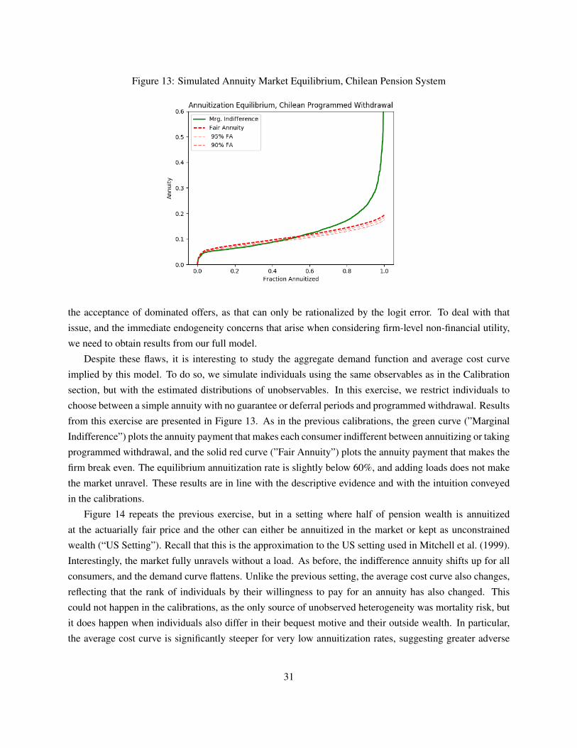
Figure 13: Simulated Annuity Market Equilibrium, Chilean Pension System

the acceptance of dominated offers, as that can only be rationalized by the logit error. To deal with that

issue, and the immediate endogeneity concerns that arise when considering firm-level non-financial utility,

we need to obtain results from our full model.

Despite these flaws, it is interesting to study the aggregate demand function and average cost curve

implied by this model. To do so, we simulate individuals using the same observables as in the Calibration

section, but with the estimated distributions of unobservables. In this exercise, we restrict individuals to

choose between a simple annuity with no guarantee or deferral periods and programmed withdrawal. Results

from this exercise are presented in Figure 13. As in the previous calibrations, the green curve (”Marginal

Indifference”) plots the annuity payment that makes each consumer indifferent between annuitizing or taking

programmed withdrawal, and the solid red curve (”Fair Annuity”) plots the annuity payment that makes the

firm break even. The equilibrium annuitization rate is slightly below 60%, and adding loads does not make

the market unravel. These results are in line with the descriptive evidence and with the intuition conveyed

in the calibrations.

Figure 14 repeats the previous exercise, but in a setting where half of pension wealth is annuitized

at the actuarially fair price and the other can either be annuitized in the market or kept as unconstrained

wealth (“US Setting”). Recall that this is the approximation to the US setting used in Mitchell et al. (1999).

Interestingly, the market fully unravels without a load. As before, the indifference annuity shifts up for all

consumers, and the demand curve flattens. Unlike the previous setting, the average cost curve also changes,

reflecting that the rank of individuals by their willingness to pay for an annuity has also changed. This

could not happen in the calibrations, as the only source of unobserved heterogeneity was mortality risk, but

it does happen when individuals also differ in their bequest motive and their outside wealth. In particular,

the average cost curve is significantly steeper for very low annuitization rates, suggesting greater adverse

31

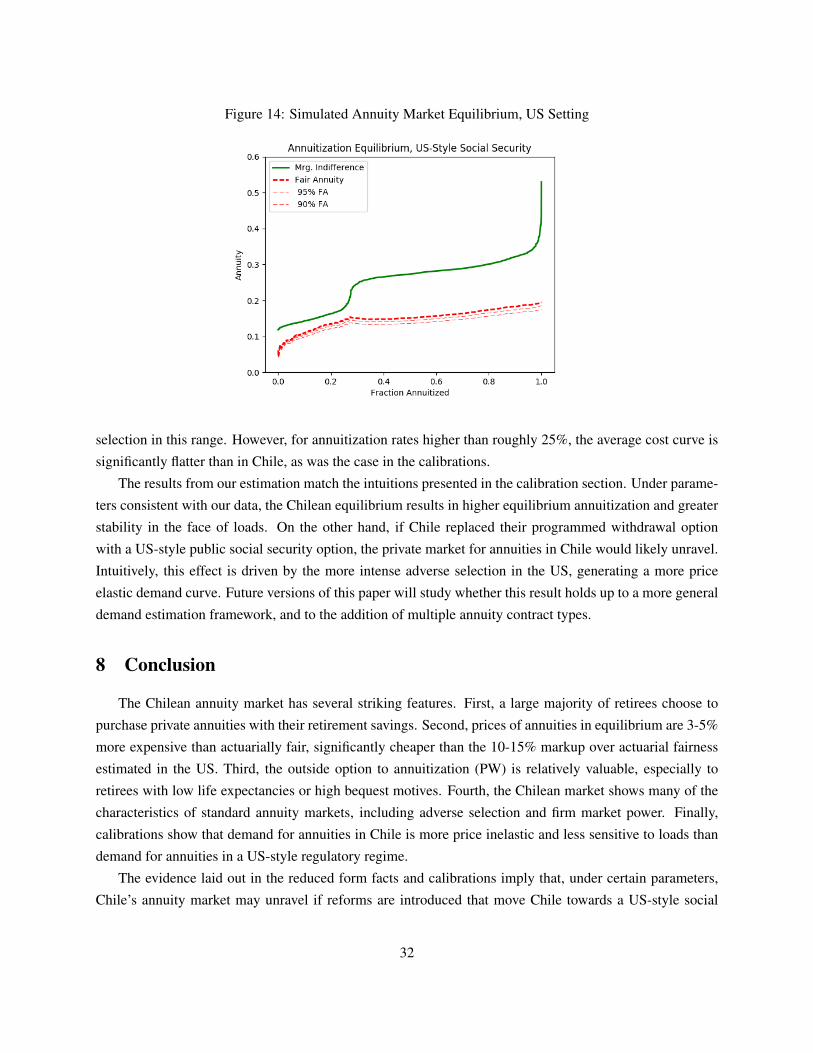
Figure 14: Simulated Annuity Market Equilibrium, US Setting

selection in this range. However, for annuitization rates higher than roughly 25%, the average cost curve is

significantly flatter than in Chile, as was the case in the calibrations.

The results from our estimation match the intuitions presented in the calibration section. Under parame-

ters consistent with our data, the Chilean equilibrium results in higher equilibrium annuitization and greater

stability in the face of loads. On the other hand, if Chile replaced their programmed withdrawal option

with a US-style public social security option, the private market for annuities in Chile would likely unravel.

Intuitively, this effect is driven by the more intense adverse selection in the US, generating a more price

elastic demand curve. Future versions of this paper will study whether this result holds up to a more general

demand estimation framework, and to the addition of multiple annuity contract types.

8 Conclusion

The Chilean annuity market has several striking features. First, a large majority of retirees choose to

purchase private annuities with their retirement savings. Second, prices of annuities in equilibrium are 3-5%

more expensive than actuarially fair, significantly cheaper than the 10-15% markup over actuarial fairness

estimated in the US. Third, the outside option to annuitization (PW) is relatively valuable, especially to

retirees with low life expectancies or high bequest motives. Fourth, the Chilean market shows many of the

characteristics of standard annuity markets, including adverse selection and firm market power. Finally,

calibrations show that demand for annuities in Chile is more price inelastic and less sensitive to loads than

demand for annuities in a US-style regulatory regime.

The evidence laid out in the reduced form facts and calibrations imply that, under certain parameters,

Chile’s annuity market may unravel if reforms are introduced that move Chile towards a US-style social

32

security system. Furthermore, the shape of the demand and average cost curves found in the calibration

exercise make it clear that simple reduced form estimation approaches are not well suited to answer this

type of question. Instead, this paper proceeds to estimate the underlying distribution of retirees’ private

information, as well as key parameters of the model, which can be used to calculate welfare and analyze

equilibrium in counterfactual regulatory regimes.

We build a structural model, based on the standard consumption-savings problem faced by retirees, that

accounts for income effects and other features of nonlinear utility that influence retirees choices. The aim is

to estimate the distribution of unobservable retiree characteristics from which we can derive their demand

for annuities and the cost firms face to insure them. The model adapts the methodology developed by Fox

et al. (2011). We pre-solve this lifecycle model for a representative set of consumers over a wide variety of

combinations of unobserved preferences. We then estimate the distribution of weights on the distribution

of consumers that allows us to match moments observed in the data. Ultimately, this will be embedded

into the micro-BLP framework, which allows us to incorporate exclusion restrictions between instruments

Z and the unobserved firm-offer component of utility. This model accounts for retirees having 1) logit

errors in valuing the financial characteristics of annuities, 2) firm preferences, and 3) characteristics that are

observable to firms but unobservable to the econometrician. Moreover, no assumptions are made about the

supply side of the market, meaning that the market may be imperfectly competitive or may be switching

across multiple equilibria.

Preliminary results show that individuals have significant and highly varied private information about

their own mortality. They also have high bequest motives, meaning that they are willing to pay for products

that provide some value to their heirs. At our estimated parameters, the Chilean equilibrium shows high

annuitization, while moving to a US-style social security system would cause the market to unravel. Fur-

ther analysis is needed to validate this result and show its robustness to different assumptions made about

demand. Our analysis shows that even though the average consumer may have high willingness to pay for

an annuity, US-style social security can push a market to unravel. Modeling both supply and demand for a

market with selection and private information and evaluating the effect of regulatory regime on equilibrium

outcomes can yield interesting results, both in the annuity context studied here, and in other areas in future

work.

References

ACKERBERG, D. A. (2009): “A new use of importance sampling to reduce computational burden in simulationestimation,” QME, 7, 343–376.

BERRY, S. (1994): “Estimating Discrete-Choice Models of Product Differentiation,” RAND Journal of Economics,25, 242–262.

BERRY, S., J. LEVINSOHN, AND A. PAKES (1995): “Automobile Prices in Market Equilibrium,” Econometrica, 63,841–90.

33

——— (2004): “Differentiated Products Demand Systems from a Combination of Micro and Macro Data: The NewCar Market,” Journal of Political Economy, 112, 68–105.

CARROLL, C. D. (2006): “The method of endogenous gridpoints for solving dynamic stochastic optimization prob-lems,” Economics Letters, 91, 312 – 320.

——— (2011): “Solution Methods for Microeconomic Dynamic Stochastic Optimization Problems,” .CHIAPPORI, P. AND B. SALANIE (2000): “Testing for Asymmetric Information in Insurance Markets,” Journal of

Political Economy, 108, 56–78.DAVIDOFF, T., J. R. BROWN, AND P. A. DIAMOND (2005): “Annuities and Individual Welfare,” American Economic

Review, 95, 1573–1590.DUBE, J.-P., J. T. FOX, AND C.-L. SU (2012): “Improving the Numerical Performance of Static and Dynamic

Aggregate Discrete Choice Random Coefficients Demand Estimation,” Econometrica, 80, 2231–2267.EINAV, L., A. FINKELSTEIN, AND P. SCHRIMPF (2010): “Optimal Mandates and the Welfare Cost of Asymmetric

Information: Evidence From the U.K. Annuity Market,” Econometrica, 78, 1031–1092.FINKELSTEIN, A. AND J. POTERBA (2014): “Testing for Asymmetric Information Using Unused Observables in

Insurance Markets: Evidence from the U.K. Annuity Market,” Journal of Risk and Insurance, 81, 709–734.FOX, J. T., K. I. KIM, S. P. RYAN, AND P. BAJARI (2011): “A simple estimator for the distribution of random

coefficients,” Quantitative Economics, 2, 381–418.FRIEDMAN, B. M. AND M. J. WARSHAWSKY (1990): “The Cost of Annuities: Implications for Saving Behavior and

Bequests,” The Quarterly Journal of Economics, 105, 135–154.ILLANES, G. (2017): “Switching Costs in Pension Plan Choice,” .KASAHARA, H. AND K. SHIMOTSU (2009): “Nonparametric Identification of Finite Mixture Models of Dynamic

Discrete Choices,” Econometrica, 77, 135–175.LOCKWOOD, L. (2012): “Bequest Motives and the Annuity Puzzle,” Review of Economic Dynamics, 15, 226–243.MITCHELL, O. S., J. M. POTERBA, M. J. WARSHAWSKY, AND J. R. BROWN (1999): “New Evidence on the

Money’s Worth of Individual Annuities,” American Economic Review, 89, 1299–1318.NEVO, A., J. L. TURNER, AND J. W. WILLIAMS (2016): “Usage-Based Pricing and Demand for Residential Broad-

band,” Econometrica, 84, 411–443.PETRIN, A. (2002): “Quantifying the Benefits of New Products: The Case of the Minivan,” Journal of Political

Economy, 110, 705–729.

A Regulatory Details

To-do: detailed description of PW payout function.

B Model

This appendix section presents the detailed explanation of how the values of annuity and programmed

withdrawal offers are calculated. It is divided into four subsections. The first derives the Euler equations

for the annuity problem; the second derives the Euler equations for the PW problem; the third presents

the computational details of how to solve the annuity problem; and the fourth does the same for the PW

34

problem.

B.1 Derivations for the Annuity Problem

Consider the problem presented in Equation 4. For expositional clarity, we ignore the no borrowing

constraint and derive a solution in an unconstrained setting, and then bring the constraint back in. It is well

known that the problems of the previous form can be re-written recursively. In any arbitrary period t, the

value of the remaining consumption problem given the current death state dt , bankruptcy state bt and liquid

assets mt is Vt(dt ,qt ,mt), and the Bellman equations are:

Vt(dt ,qt ,mt) = maxct(dt ,qt)

ct(dt ,qt)1−γ

1− γ+δ ·Γt(dt ,qt)

′

Et [Vt+1(0,0,mt+1)]

Et [Vt+1(0,1,mt+1)]

Et [Vt+1(1,0,mt+1)]

Et [Vt+1(1,1,mt+1)]

(39)

where Γt(0,0)=

(1−µt+1)(1−ψt+1)

(1−µt+1)ψt+1

µt+1(1−ψt+1)

µt+1ψt+1

, Γt(0,1)=

0

(1−µt+1)

0

µt+1

, Γt(1,0)=

0

0

(1−ψt+1)

ψt+1

, and Γt(1,1)=

0

0

0

1

, and each equation is subject to the appropriate dynamic budget constraints and transition rules. We

can simplify the previous equation by noting that there is no optimization after death, so for the absorbing

state (dt = 1,qt = 1) we have that:

Vt(1,1,mt) = β[mt +PDV z

t (1,1,D,G)]1−γ

1− γ

Et [Vt+1(1,1,mt+1)] = β

[mt+1 +PDV z

t+1(1,1,D,G)]1−γ

1− γ(40)

where PDV zt (1,1,D,G) = ∑

G+Dτ=t+1 Rt−τ · zτ(1,1,D,G) is the PDV in period t of the payment stream of the

guarantee period from t +1 to G+D.

The expressions are similar in the ”dead but not bankrupt” case (dt = 1,qt = 0), but take into account

that for guaranteed annuities there is uncertainty in the value of future payments:

Vt(1,0,mt) = β[mt +E[PDV z

t (1,0,D,G)]]1−γ

1− γ

Et [Vt+1(1,0,mt+1)] = β

[mt+1 +E[PDV z

t+1(1,0,D,G)]]1−γ

1− γ(41)

35

where E[PDV zt (1,0,D,G)] is the expected present value in t of the payment stream of the guarantee period

from t +1 to G+D:

E[PDV zt (1,0,D,G)] =

G+D

∑τ=t+1

Rt−τ · ((1−Ψτ) · zτ(1,0,D,G)+Ψτ · zτ(1,1,D,G)) (42)

Ψτ =τ

∑κ=t+1

(κ−1

∏κ=t+1

(1−ψκ)

)ψκ (43)

and Ψτ is the probability that the firm is bankrupt in τ > t, conditional on not being bankrupt in t.

As for the remaining states (when the individual is alive), the FOCs from (39) are:

ct(0,qt)−γ = δ ·R ·Γt(0,qt)

′

Et[V ′t+1(0,0,mt+1)

]Et[V ′t+1(0,1,mt+1)

]Et[V ′t+1(1,0,mt+1)

]Et[V ′t+1(1,1,mt+1)

]

(44)

We know that:

Et[V ′t+1(1,0,mt+1)

]= β · [mt+1 +

G+D

∑τ=t+1

Rt−τ · ((1−Ψτ) · zτ(1,0,D,G)+Ψτ · zτ(1,1,D,G))]−γ

Et[V ′t+1(1,1,mt+1)

]= β ·

[mt+1 +

G+D

∑τ=t+1

Rt−τ · zτ(1,1,D,G)

]−γ

(45)

Also, from the Envelope Theorem:

V ′t (0,qt ,mt) = δ ·R ·Γt(0,qt)′

Et[V ′t+1(0,0,mt+1)

]Et[V ′t+1(0,1,mt+1)

]Et[V ′t+1(1,0,mt+1)

]Et[V ′t+1(1,1,mt+1)

]

(46)

Combining (44) and (46), and rolling the equation forward by one year:

ct(0,qt)−γ =V ′t (0,qt ,mt)

ct+1(0,qt+1)−γ =V ′t+1(0,qt+1,at ·R+ zt+1(0,qt+1,D,G)) (47)

36

Substituting back into (44) yields the Euler equation:

ct(0,qt)−γ = δ ·R ·Γt(0,qt)

′

Et [ct+1(0,0)−γ ]

Et [ct+1(0,1)−γ ]

Et[V ′t+1(1,0,mt+1)

]Et[V ′t+1(1,1,mt+1)

]

(48)

Following Carroll (2012), note that in equation (47) neither mt nor ct has any direct effect on V ′t+1. Instead,

it is their difference, at , which enters into the function. This motivates the use of the Endogenous Gridpoint

Method to approximate the optimal policy and value functions, as is derived in subsection B.3. Before

moving to computation, however, the next section presents the analogous derivation for the PW problem.

B.2 Derivations for the PW Problem

Consider for now the problem free of borrowing constraint. As before, utility is CRRA, and in each

state is given by:

u(ct ,dt = 0) =c1−γ

t

1− γ

u(dt = 1) = β · (mt +PWt)1−γ

1− γ(49)

As in the annuity case, to obtain the value of taking a PW offer we re-write the problem in recursive form.

The Bellman equation for the PDV of expected utility under the optimal state-contingent consumption path,

for any period t, given the death state, PW account balance, and asset balance, denoted by Vt(dt ,PWt ,mt),

is:

Vt(dt = 0,PWt ,mt) = maxct

c1−γ

t

1− γ+δ ·Γ′t

[Et [Vt+1(0,mt+1,PWt)]

Et [Vt+1(1,mt+1,PWt)]

](50)

where Γt =

[1−µt+1

µt+1

]and, as before, the problem is constrained by dynamic budget constraints and tran-

sition rules. Since there is no optimization after death, and inheritors receive the full PW balance, for the

absorbing state dt = 1 we have that:

Vt(1,mt ,PWt) = β[mt +PWt ]

1−γ

1− γ(51)

Therefore we can write the expected continuation value for the death state as:

Et [Vt+1(1,mt+1,PWt)] =β

1− γ

∫ [mt+1 +(PWt − zt(PWt)) ·RPW ]1−γ

dF(RPW ) (52)

37

For the state where the individual is alive, the expected continuation value is:

Et [Vt+1(0,mt+1,PWt)] =∫

Vt+1(0,(PWt − zt(PWt)) ·RPW ,mt+1)dF(RPW ) (53)

With these definitions, the FOCs from (50) are:

c−γ

t = δ ·R ·Γ′t

[Et[V ′t+1(0,mt+1,PWt)

]Et[V ′t+1(1,mt+1,PWt)

]] (54)

We know that:

Et[V ′t+1(1,mt+1,PWt)

]= β ·R

∫ [mt+1 +(PWt − zt(PWt)) ·RPW ]−γ

dF(RPW ) (55)

Also, from the Envelope Theorem:

V ′t (0,mt) = δ ·R ·Γ′t

[Et[V ′t+1(0,mt+1,PWt)

]Et[V ′t+1(1,mt+1,PWt)

]] (56)

Combining (54) and (56), and rolling the equation forward by one year:

c−γ

t =V ′t (0,mt)

c−γ

t+1 =V ′t+1(0,mt+1,PWt+1) (57)

Substituting back into (54) yields the Euler equation:

c−γ

t = δ ·R ·Γ′t

[Et

[c−γ

t+1

]Et[V ′t+1(1,mt+1,PWt)

]] (58)

B.3 Computation of the Solution to the Annuity Problem

Having derived the conditions that govern the optimal consumption policy and the value functions for

both problems, this subsection presents the details of the numerical procedure used to solve these conditions.

Since the problem is solved recursively, we will begin with the solution for period T and work our way

backwards. In period T , µT = 1 and T > G+D, so mT = aT−1 ·R and regardless of the bankruptcy state qT :

VT (0,qT ,mT ) = β · m1−γ

T1− γ

(59)

Then in the next-to-last period:

VT−1(0,qT−1,mT−1) = maxcT−1

c1−γ

T−1

1− γ+δ ·β · ((mT−1− cT−1) ·R)1−γ

1− γ(60)

38

Which generates the optimal policy:

c−γ

T−1 = δ ·β ·R1−γ · (mT−1− cT−1)−γ

cT−1(0,qT−1,mT−1) =R

((δ ·β ·R)1γ +R)

·mT−1 (61)

And implies that the value function in T −1 is:

VT−1(0,qT−1,mT−1) =

(1+(δ ·β ·R1−γ)1/γ

1− γ

)(R ·mT−1

(δ ·β ·R)1/γ +R

)1−γ

(62)

Note that conditional on mT−1, there is no dependence on qT−1. That is, qT−1 will shift mT−1, as mT−1 =

aT−2 ·R+ zT−1(0,qT−1,D,G), but conditional on mT−1 it becomes irrelevant. Therefore, given a grid of

mT−1 one could easily solve for VT−1(mT−1), and the value of mT−1’s for other values would be found by

interpolation/extrapolation. Note as well that as long as the bequest motive is positive the no-borrowing

constraint can be omitted from this stage without loss as the the unconstrained solution always satisfies

cT−1 < mT−1.

Having solved for all the relevant quantities in T − 1 and T , let us consider the unconstrained problem in

T −2. From the Euler condition in (48) and the optimal policy in (61):

cT−2(0,qt)−γ = δ ·R ·ΓT−2(0,qt)

′

Et [cT−1(0,0)−γ ]

Et [cT−1(0,1)−γ ]

Et[V ′T−1(1,0,mT−1)

]Et[V ′T−1(1,1,mT−1)

]

= δ ·R ·ΓT−2(0,qt)′

(R

((δ ·β ·R)1/γ+R)

)−γ

((mT−2− cT−2(0,qT−2)) ·R+ zT−1(0,0,D,G))−γ(R

((δ ·β ·R)1/γ+R)

)−γ

((mT−2− cT−2(0,qT−2)) ·R+ zT−1(0,1,D,G))−γ

β ·[(mT−2− cT−2(0,qT−2)) ·R+ zT−1(1,0,D,G)+E[PDV z

T−1(1,0,D,G)]]−γ

β ·[(mT−2− cT−2(0,qT−2)) ·R+ zT−1(1,1,D,G)+E[PDV z

T−1(1,1,D,G)]]−γ

Unfortunately, this is a non-linear system of equations. To find the value function in T −2, one could fix a

grid of mT−2, and for each point in the grid solve for optimal consumption and obtain the value function.

Interpolation across m’s would yield the value function for any mT−2. Note also that the previous derivation

is also valid for 0 < t < T −2, so backward induction would allow us to unwind this problem and construct

the value function in period 1. The problem in period 0 is slightly different, as the state is (0,0) and wealth

is ω + z0(0,0,D,G)+FDA with certainty29, but the same tools apply.

One issue we’ve abstracted away from up to now is the no-borrowing constraint: aT−1 ≥ 0. Incorporat-

29Recall that FDA is the free disposal amount, another attribute of an annuity offer. In most cases, it is 0.

39

ing this constraint implies that when mT−1 is sufficiently low, consumption will not be the solution to the

aforementioned problem, but rather mT−1 itself. This creates a discontinuity in the optimal policy function.

Since our approximations to the optimal policy and value functions are constructed by interpolation, it is

crucial to incorporate the point where the discontinuity takes place into the grid of points to be evaluated.

This ensures that the no-borrowing constraint is properly accounted for in the model. At the point where the

no-borrowing constraint binds, mT−1, the marginal value of consuming mT−1 must be equal to the marginal

utility of saving 0.

We use the Endogenous Gridpoints Method (Carroll (2006)) to find the solution to the aforementioned prob-

lem. At a high level, the strategy is to solve the model for a grid of asset states, and then to interpolate across

states to obtain the policy function and the value function. EGM allows us to solve the model efficiently,

by re-writing the problem in a way that allows us to back out a solution using an inversion rather than root-

finding. The details of the implementation for T −2 are presented below:

Numerical Calculation of Policy Function in T −2:

1. Select a grid of aT−2 with support [0, aT−2], where:

aT−2 = RT−2ω +

T−2

∑τ=0

RT−2−τzτ(0,0,D,G) (63)

40

2. Calculate the relevant quantities for the unconstrained problem:

mT−1(dT−1,qT−1,D,G) = aT−2 ·R+ zT−1(dT−1,qT−1,D,G)) (64)

cT−1(0,qT−1) =

(R

((δ ·β ·R)1/γ +R)·mT−1(0,qT−1,D,G)

)−γ

(65)

cT−2(0,qT−2) =

δ ·R ·ΓT−2(0,qT−2)′

cT−1(0,0)

cT−1(0,1)

β · [mT−1(1,0,D,G)]−γ

β · [mT−1(1,1,D,G)]]−γ

− 1

γ

(66)

cT−2(0,qT−2) = cT−2(0,qT−2)−γ (67)

mT−2(0,qT−2) = cT−2(0,qT−2)+aT−2 (68)

VT−1(0,qT−1) =

(1+(δ ·β ·R1−γ)1/γ

1− γ

)(R ·mT−1(0,qT−1)

(δ ·β ·R)1/γ +R

)1−γ

(69)

VT−1(1,qT−1) = β

(mT−1(1,qT−1)

1−γ

1− γ

)(70)

VT−2(0,qT−2) =cT−2(0,qT−2)

1−γ

1− γ+δ ·ΓT−2(0,qT−2)

VT−1(0,0)

VT−1(0,1)

VT−1(1,0)

VT−1(1,1)

(71)

3. Denote mT−2(0,qT−2) the solution to equation (68) when aT−2,i = 0. This is the lowest level of wealth

that is unconstrained. Define

VT−1(0,qT−1) =

(1+(δ ·β ·R1−γ)1/γ

1− γ

)(R · zT−1(0,qT−1,D,G)

(δ ·β ·R)1/γ +R

)1−γ

(72)

VT−1(1,qT−1) = β

(zT−1(1,qT−1,D,G)1−γ

1− γ

)(73)

cT−2, j(0,qT−2) = m−γ

T−2, j (74)

VT−2, j(0,qT−2,mT−2) =m1−γ

T−2, j

1− γ+δ ·ΓT−2(0,qT−2)

VT−1(0,0)

VT−1(0,1)

VT−1(1,0)

VT−1(1,1)

(75)

4. Use interpolation to obtain cT−2(0,qT−2,mT−2), `cT−2, j(0,qT−2), VT−2,(0,qT−2,mT−2), and `VT−2,(0,qT−2,mT−2)

for the unconstrained problem.

5. Correct for the no-borrowing constraint by constructing a part exact, part interpolated policy and value

41

function for this period 30

c∗T−2(0,qT−2,mT−2) =

m−γ

T−2 if mT−2 < mT−2(0,qT−2)

cT−2(0,qT−2,mT−2) otherwise

V ∗T−2(0,qT−2,mT−2) =

VT−2,(0,qT−2,mT−2) if mT−2 < mT−2(0,qT−2)

VT−2,(0,qT−2,mT−2) otherwise

There are three issues worth discussing in this procedure: first, we assume that individuals cannot borrow

against future annuity payments (the lower bound of a is 0). This is consistent with our knowledge of the

Chilean banking system. Second, we set the upper bound of the support of assets as the PDV of initial

wealth plus the PDV of the maximum sequence of previous annuity payments. This ensures that the grid of

a’s spans the optimal asset value in T −2, as in the model the agent cannot accumulate more wealth than this

value. Third, we interpolate over c(·) instead of c(·). This is suggested by Carroll (2011), as the function

that enters into the recursion in earlier periods is c(·), and not c(·). One could interpolate over c(·), and then

raise the interpolated value to the power of −1γ, but that is less accurate is simply interpolating over c. With

these objects, we can solve the problem for T −3,T −4, ...,0 by recursion.

Numerical Calculation of Policy Function in t:

1. Select a grid of at with support [0, at ]:

at = Rtω +

t

∑τ=0

Rt−τzτ(0,0,D,G) (76)

2. Calculate the relevant quantities for the unconstrained problem (suppressing the dependence on D and

30Note that the solution objects for the T −2 problem are exact when the constraint binds.

42

G to simplify notation):

mt+1(0,qt+1) = at ·R+ zt+1(0,qt+1) (77)

ct(0,qt) =

δ ·R ·Γt(0,qt)′

c∗t+1(0,0,mt+1(0,0))

c∗t+1(0,1,mt+1(0,0))

β ·[mt+1(1,0)+E[PDV z

t+1(1,0,D,G)]]−γ

β ·[mt+1(1,1)+E[PDV z

t+1(1,1,D,G)]]−γ

− 1

γ

(78)

ct(0,qT−2) = ct(0,qT−2)−γ (79)

mt(0,qt) = ct(0,qt)+at (80)

Vt+1(1,qt+1) = β

(mt+1(1,qt+1)

1−γ

1− γ

)(81)

Vt(0,qt) =ct(0,qt)

1−γ

1− γ+δ ·Γt(0,qt)

V ∗t+1(0,0,mt+1)

V ∗t+1(0,1,mt+1)

Vt+1(1,0)

Vt+1(1,1)

(82)

3. Define mt(0,qt) as the level of wealth obtained at at = 0 and

Vt+1(1,qt+1) = β

(E[PDV z

t+1(1,qt+1,D,G)]1−γ

1− γ

)(83)

Vt(0,qt) =mt(0,qt)

1−γ

1− γ+δ ·ΓT−2(0,qT−2)

V ∗t+1(0,0,zt+1(0,0))

V ∗t+1(0,1,zt+1(0,1))

Vt+1(1,0)

Vt+1(1,1)

(84)

4. Use interpolation to obtain ct(0,qt ,mt), `ct, j(0,qt), Vt,(0,qt ,mt), and `Vt,(0,qt ,mt) for the unconstrained

problem.

5. Correct for the no-borrowing constraint:

c∗t (0,qt ,mt) =

m−γ

t if mt < mt(0,qt+1)

ct(0,qt ,mt) otherwise

V ∗t (0,qt ,mt) =

Vt(0,qt ,mt) if mt < mt(0,qt)

Vt(0,qt ,mt) otherwise

6. Repeat for t−1

Note that again, the constrained segment requires no additional interpolation and hence its implemen-

tation is both efficient and precise.We can recover the object of interest (the value of an annuity offer:

43

V (0,0,ωi,D,G)) after the t = 0 step in the previous recursion.

B.4 Computation of the Solution to the PW Problem

In period T , µT = 1 and PWT = 0, so mT = aT−1 ·R and:

VT (0,mT ,PWT ) = β · m1−γ

T1− γ

(85)

Then in the next-to-last period:

VT−1(0,mT−1,PWT−1) = maxcT−1

c1−γ

T−1

1− γ+

δ ·β1− γ

((mT−1− cT−1) ·R)1−γ (86)

The optimal policy and value functions in T −1 are then:

cT−1(mT−1) =R

((δ ·β ·R)1γ +R)

·mT−1 (87)

VT−1(0,mT−1) =

(1+(δ ·β ·R1−γ)1/γ

1− γ

)(R ·mT−1

(δ ·β ·R)1/γ +R

)1−γ

(88)

Note that, conditional on mT−1, there is no dependence on PWT−1. This is because PWT−1 will shift mT−1,

as mT−1 = aT−2 ·R+ zT−1(PWT−1,a), but conditional on mT−1 it becomes irrelevant. Additionally, as in

the annuity problem, as long as the bequest motive is not negative the unconstrained maximizer satisfies the

no-borrowing constraint.

Having solved for all the relevant quantities in T −1 and T , we can proceed to solve the problem in T −2.

There are a few additional objects that need to be introduced before proceeding. First, take K draws from

the distribution of RPW . Each draw will be denoted by k, and draws will be held fixed across time periods.

Define RK as the largest draw from the distribution of RPW . Second, define the upper bound of the grid of

PW, ¯PW , recursively:

¯PW 1 = RK · (PW0− zt(PW0))

¯PW t = RK · ( ¯PW t−1− zt( ¯PW t−1)) (89)

Finally, define the upper bound of the grid of accumulated assets as:

at = Rtω +

t

∑τ=0

Rt−τz( ¯PWτ ,0, f ) (90)

Numerical Calculation of Policy Function in T −2:

44

1. Select a grid of (aT−2,i,PWT−2,i) with support [0, aT−2]× [0, ¯PW T−2].

2. Calculate the relevant quantities for the unconstrained problem:

mT−1,k(0) = aT−2 ·R+ zT−1(RPWk · (PWT−2− z(PWT−2),0,a) (91)

mT−1,k(1) = aT−2 ·R+RPWk · (PWT−2− z(PWT−2)) (92)

ET−2[cT−1] =1K

K

∑k=1

[cT−1(mT−1,k(0))]−γ (93)

ET−2[V ′T−1(1)] =β

K

K

∑k=1

[mT−1,k(1)]−γ (94)

cT−2 =

[δ ·R ·Γ′T−2

[ET−2[cT−1]

ET−2[V ′T−1(1)]

]]− 1γ

(95)

mT−2 = cT−2 +aT−2 (96)

cT−2 = c−γ

T−2 (97)

ET−2[VT−1(0)] =

(1+(δ ·β ·R1−γ)1/γ

1− γ

)·(

R(δ ·β ·R)1/γ +R

)1−γ 1K

K

∑k=1

[mT−1,k(0)]1−γ (98)

ET−2[VT−1(1)] =β

1− γ· 1

K

K

∑k=1

[mT−1,k(1)]1−γ (99)

VT−2 =c1−γ

T−2

1− γ+δ ·Γ′T−2

[ET−2[VT−1(0)]

ET−2[VT−1(1)]

](100)

3. Denote mT−2(PWT−2) the solution to (96) when aT−2 = 0 and the PW balance is PWT−2 define

VT−2(mT−2,PWT−2) =m1−γ

T−2

1− γ+δ ·Γ′T−2

[ET−2[VT−1(0)]

ET−2[VT−1(1)]

](101)

with the value of VT−1 determined by aT−2 = 0.

4. Use interpolation to obtain cT−2(mT−2,PWT−2) and VT−2(0,mT−2,PWT−2) for the unconstrained

problem. Form the boundary interpolator `mT−2(PWT−2) which determines the minimum level of

unconstrained wealth for each value of the PW balance.

5. Correct for the no-borrowing constraint by constructing a part exact, part interpolated policy and value

function for this period 31

c∗T−2(mT−2,PWT−2) =

m−γ

T−2 if mT−2 < `mT−2(PWT−2)

cT−2(mT−2,PWT−2) otherwise

31Note that the solution objects for the T −2 problem are exact when the constraint binds.

45

V ∗T−2(mT−2,PWT−2) =

VT−2,(mT−2,PWT−2) if mT−2 < `mT−2(PWT−2)

VT−2,(mT−2,PWT−2) otherwise

Armed with these objects, we can solve the problem for T −3,T −4, ...,0 by recursion.

Numerical Calculation of Policy Function in t:

1. Select a grid of (at ,PWt) with support [0, at ]× [0, ¯PW t ].

2. Calculate the relevant quantities for the unconstrained problem:

mt+1,k(0) = at ·R+ zt+1(RPWk · (PWt − zt(PWt)),0,a) (102)

mt+1,k(1) = at ·R+RPWk · (PWt − zt(PWt)) (103)

Et [ct+1] =1K

K

∑k=1

`ct+1(mt+1,k(0),PWt+1,k) (104)

Et [V ′t+1(1)] =β

K

K

∑k=1

[mt+1,k(1)]−γ (105)

ct =

[δ ·R ·Γ′t

[Et [ct+1]

Et [V ′t+1(1)]

]]− 1γ

(106)

mt = ct +at,i (107)

ct = c−γ

t (108)

Et [Vt+1(0)] =1K

K

∑k=1

V (0,mt+1,k(0),RPWk · (PWt − z(PWt))) (109)

Et [Vt+1(1)] =β

1− γ· 1

K

K

∑k=1

[mt+1,k(1)]1−γ (110)

Vt =c1−γ

t

1− γ+δ ·Γ′t

[Et [Vt+1(0)]

Et [Vt+1(1)]

](111)

3. Denote mt(PWt) the solution when at = 0 and the PW balance is PWt define

Vt(mt ,PWt) =m1−γ

t

1− γ+δ ·Γ′t

[Et [Vt+1(0)]

Et [Vt+1(1)]

](112)

with the value of Vt+1 determined by at = 0.

4. Use interpolation to obtain ct(mt ,PWt) and Vt(0,mt ,PWt) for the unconstrained problem. Form the

boundary interpolator `mt(PWt) which determines the minimum level of unconstrained wealth for each

value of the PW balance.

46

5. Correct for the no-borrowing constraint by constructing a part exact part interpolated policy and value

function for this period:

c∗t (mt ,PWt) =

m−γ

t if mt < `mt(PWt)

ct(mt ,PWt) otherwise

V ∗t (mt ,PWt) =

Vt,(mt ,PWt) if mt < `mt(PWt)

Vt,(mt ,PWt) otherwise

6. Repeat for t−1

We can recover the object of interest (the value of a PW offer: V0(0,ω,PW0)) after the t = 0 step in the

previous recursion.

C Appendix Tables and Figures

010

2030

4050

Num

ber o

f Ret

irees

01jan2005 15jan2005 29jan2005 12feb2005 26feb2005Date

Number of Retirees by Date, First Table Change

Figure 15: Number of retirees by date, around the first mortality table change in our data

47

010

2030

40N

umbe

r of R

etire

es

04jun2010 18jun2010 02jul2010 16jul2010 30jul2010Date

Number of Retirees by Date, Second Table Change

Figure 16: Number of retirees by date, around the second mortality table change in our data

48