Competing Theories of Financial Anomalies

Alon Brav* and J. B. Heaton**

First Draft: August 1999 This Draft: April 2000

Abstract

We compare two competing theories of financial anomalies: (1) “behavioral” theories relying oninvestor irrationality; and (2) rational “structural uncertainty” theories relying on investoruncertainty about the structure of the economic environment. Each relaxes the traditional rationalexpectations theory differently. However, the resulting theories are virtually indistinguishableempirically, even as their normative implications differ radically. Given their mathematical andpredictive similarities, we argue that attention should shift from the behavioral-rational debatetoward a greater (and perhaps less philosophical) focus on investor concern with structuraluncertainty. An approach that integrates traditionally rational modeling methods with greateremphasis on the psychology of structural uncertainty offers a plausible economic context for theappearance of behaviors emphasized in behavioral finance, and may help economists betterunderstand when those behaviors might be important. We illustrate this approach by developing aBayesian structural uncertainty model of “overconfidence” (excessive certainty) supported by theexisting psychological literature and easily linked with current behavioral finance research.

* Assistant Professor of Finance, Duke University Fuqua School of Business.** Associate, Bartlit Beck Herman Palenchar & Scott (Chicago).

This paper has benefited from discussions with Nick Barberis, Eli Berkovitch, Craig Fox, John Graham, CampbellHarvey, Harrison Hong, Arthur Kraft, Pete Kyle, Jonathan Lewellen, Mark Mitchell, John Payne, Nick Polson,Nathalie Rossiensky, Jakob Sagi, Andrei Shleifer, Steve Tadelis, Richard Thaler, Rob Vishny, TuomoVuolteenaho, Bob Whaley, Richard Willis, and participants at the 1999 Cornell Summer Finance Conference,Duke, MIT, Rice, the University of North Carolina Mini-Conference on Behavioral Finance, and the Society ofFinancial Studies/Kellogg Conference on Market Frictions and Behavioral Finance. Please address correspondenceto Brav at Fuqua School of Business, Duke University, Box 90120, Durham, North Carolina 27708, phone: (919)660-2908, email: brav@mail.duke.edu or Heaton at Bartlit Beck Herman Palenchar & Scott, 54 West HubbardStreet, Chicago, Illinois 60610, phone (312) 494-4425, email: jb.heaton@bartlit-beck.com.

1

Competing Theories of Financial AnomaliesTraditional efficient markets/rational expectations asset pricing models have difficulty

explaining available empirical evidence.1 Two distinct assumptions characterize those models: (1)

completely rational information processing, and (2) complete knowledge of the fundamental

structure of the economy.2 Put another way, investors in traditional rational expectations asset

pricing models were supposed to “get it right” because they had "access both to the correct

specification of the 'true' economic model and to unbiased estimators of its coefficients"

[Friedman (1979, p. 38)]. Not surprisingly, to explain why investors sometimes “get it wrong,”

financial economists have relaxed these two assumptions. In doing so, they have created two

competing sets of theories to explain “financial anomalies.”

First, and probably best known, are behavioral explanations that relax the first assumption

(completely rational information processing) and "entertain the possibility that some of the agents

in the economy behave less than fully rationally some of the time" [Thaler (1993, p. xvii)]. In

behavioral theories, investors do not process available information rationally because they suffer

from cognitive biases. The (often implicit) background assumption is that although irrational

investors fail to process information rationally, they have considerable structural knowledge about

the economy. This is generally consistent with the experimental results that motivate behavioral

1 Researchers continue to adjust traditional rational expectations models to better fit the data, usually by modifyingstandard preference structures. See, for example, Barberis, Huang, and Santos (1999), Campbell and Cochrane(1999), and Constantinides (1990). Such models are rational expectations models in all respects, and thus do not fitinto the classes of models with which we are concerned here: those that relax rational expectations in some way.2 There are numerous ways to state this assumption. In models with a representative agent, the second assumptionrequires that the agent knows the true model underlying the economy. In models with heterogeneous agents, theassumption requires “consistency between individuals’ choices and what their perceptions are of aggregatechoices” [Sargent (1993, p. 7)]. The possibility of attaining such a structural knowledge within a rationalexpectation equilibrium is by no means guaranteed and has received considerable attention [see Blume and Easley(1982), Bray and Savin (1984), and Bray and Kreps (1987)].

2

finance. Subjects tend to exhibit cognitive biases in psychological experiments despite their ability

to observe relevant data generating processes.3

Shiller (1981) is an early example attributing financial anomalies to irrationality, finding

evidence that stock prices move too much to be consistent with news about future dividends.

DeBondt and Thaler (1985) use psychological evidence to motivate a price overreaction

hypothesis. They find (in apparent violation of weak-form market efficiency) that stocks with past

extreme bad returns outperform stocks with past extreme good returns. Lakonishok, Shleifer, and

Vishny (1994) find that portfolios formed on the basis of publicly-available accounting and price

data earn superior returns. Their results are consistent with extrapolation of past operating

performance into the future. A number of recent papers have added greater theoretical content to

this literature. Daniel, Hirshleifer, and Subrahmanyam (1998) generate overreaction and

underreaction4 from investors' overconfidence in their private signals and biased updating in light

of public information. Barberis, Shleifer, and Vishny (1998) study the same anomalies by

modeling a representative investor subject to two cognitive biases. Hong and Stein (1999) study

the interaction of traders who naively follow price trends and traders who naively study

fundamental news.

A second set of theories maintains the complete rationality assumption but relaxes the

assumption that investors have complete knowledge of the fundamental structure of the economy.

To appreciate this approach, it is crucial to note that axiomatic rationality (that is, following

3 See, for example, Grether (1980) who finds evidence of cognitive biases in an incentive-compatible environmentwith observable bingo-cage data generating mechanisms. Indeed, the fact that cognitive biases arise inenvironments where the optimal strategy should be relatively easy to determine, given the observability of datagenerating mechanisms, is precisely what lends these results such force for many economists.

3

rational decision making rules like Bayes’ Theorem when dealing with uncertainty) is a necessary,

but not sufficient, condition for a “rational expectations” model, at least insofar as that term is

used in a technical sense. As Friedman (1979) explains, the distinction between axiomatic

rationality and rational expectations is the distinction between information exploitation and

information availability. Rational investors in a rational expectations world not only exploit all

available information in a perfectly rational manner; the set of information available to them is the

full set of relevant information.5 Axiomatically rational investors who live outside a rational

expectations world use all information available to them in a perfectly rational way (e.g., by

following Bayes’ Theorem whenever they face uncertainty), but simply do not have all relevant

information about the economy. “Rational structural uncertainty” models, as we will refer to

them, generate financial anomalies from mistakes or risk premiums that result when rational

investors remain critically uninformed about their economic environment.

For example, Merton (1987) presents a model of capital market equilibrium where a given

investor is informed only about a subset of all securities, showing why, for example, the small-firm

effect might arise in such a world. Lewis (1989) argues that dollar forecast errors during the

1980s could have resulted from investors' prior beliefs that the change in U.S. money demand

would not persist and subsequent learning about the true process generating fundamentals.

Timmerman (1993) analyzes a representative investor who must learn dividend growth rates to

4 "Overreaction" refers to the predictability of good (bad) future performance from bad (good) past performance[see, for example, DeBondt and Thaler (1985) and Lakonishok, Shleifer, and Vishny (1994)]. "Underreaction"refers to the predictability of good (bad) future performance from good (bad) past performance [see, for example,Jegadeesh and Titman (1993), Michaely, Thaler, and Womack (1995), Chan, Jegadeesh, and Lakonishok (1996)].5 As Kurz (1994, pp. 877-78) states: “[T]he theory of rational expectations in economics and game theory is basedon the premise that agents know a great deal about the basic structure of their environment. In economics agentsare assumed to have knowledge about demand and supply functions, of how to extract present and future generalequilibrium prices, and about the stochastic law of motion of the economy over time. … [T]hese agents possess‘structural knowledge.’” (emphasis in original)

4

price securities, and shows that least-squares learning can generate volatility and predictability.

Barsky and DeLong (1993) take up the problem of the rational investor who must estimate an

unknown and possibly nonstationary dividend growth rate, showing that a simple learning process

generates stock market volatility that is highly consistent with the data. Kurz (1994) presents an

intricate theory of expectations formation under the assumption that agents do not know the

structural relations of the economy. In his model, resulting beliefs are “rational” so long as they

are consistent with the observed past data, though numerous different beliefs may be compatible

when the structure is non-stationary. Morris (1996), following Miller (1977), presents a model

where different Bayesian prior beliefs about an asset’s expected cash flows lead to the patterns of

underperformance associated with initial public offerings. More recently, Lewellen and Shanken

(1999) examine an economy populated by rational Bayesian investors who posses imperfect

knowledge regarding valuation-relevant parameters, showing how asset prices will exhibit

predictability, excess volatility, and deviations from the CAPM as these investors update their

beliefs. Also following the structural uncertainty approach are several recent and related papers by

Anderson, Hansen, Sargent (1999), Hansen, Sargent and Tallarini (2000), and Hansen, Sargent

and Wang (2000), who present models where agents are concerned with model misspecification.

In these models agents do not know the true model that actually generates the data, and attempt

to apply robust decision rules. The introduction of such model uncertainty allows these authors to

derive new implications for a wide range of asset pricing questions such as the magnitude of the

equity premium and consumption and saving rules.

Our paper presents a comparative analysis of these theories. Having stressed how each

embodies a different deviation from the rational expectations ideal, we illustrate both sets of

theories in simple models generating two financial anomalies: overreaction and underreaction. We

5

use the well-known cognitive biases of “conservatism” and the “representativeness heuristic” to

motivate the behavioral models in our comparative analysis. Both are deviations from optimal

Bayesian judgment that have enjoyed application in behavioral finance. In our rational structural

uncertainty approach, we model a Bayesian (i.e., rational) investor with uncertainty about the

stability of the valuation-relevant parameter. We employ Bayesian change-point analysis [see

Smith (1975)] to produce an optimal estimator for this structurally uncertain environment.

We next ask whether these theories can be distinguished empirically. Our conclusions are

not encouraging. Because they share striking mathematical and predictive similarities, it is

extremely difficult to distinguish these theories empirically. We illustrate this difficulty in two

ways. First, we show how the rational structural uncertainty model, though built on a completely

Bayesian foundation, embodies the two essential features of the behavioral models— heavy

weighting of prior opinion and heavy weighting of recent data. Similar use of data and prior

beliefs makes distinguishability hard.

Second, we show why the predictions from these theories are equally consistent with

available empirical evidence. We highlight an unemphasized feature of the empirical studies that

document overreaction and underreaction. Empirical studies finding overreaction [see, for

example, DeBondt and Thaler (1985); Lakonishok, Shleifer, and Vishny (1994)] study economic

environments very different from empirical studies finding underreaction [see, for example,

Jegadeesh and Titman (1993), Michaely, Thaler, and Womack (1995), Chan, Jegadeesh, and

Lakonishok (1996)]. Overreaction studies have focused on firms in relatively stable environments

(firms with a long history of poor performance or good performance), while underreaction studies

have focused on firms at and after “extreme” periods (for example, after extreme returns, earnings

surprises, dividend initiation or omission, etc.). It is easy to select cognitive biases that might

6

account for price behavior in each of the environments. However, these are also the selected

environments where even a perfectly rational Bayesian concerned with structural change can

exhibit behavior that will lead to “overreaction” to recent data in a stable environment, and

“underreaction” to a structural break when the location of a break is not known with certainty.6

The predictive similarity of the two theories is troubling because the theories have very

different normative consequences. Perhaps most importantly, implications for capital market

regulatory policy differ under each approach. It is much easier to make a case for paternalistic

governmental intervention under a behavioral view where traders make mental errors than under a

structural uncertainty approach where traders are doing their rational best. Even proponents of

the behavioral view recognize, however, that regulators and lawmakers may suffer from biases as

well [see, for example, Jolls, Sunstein, and Thaler (1998)]. Even if they do not, rational regulators

subject to structural uncertainty may be unable to distinguish periods of irrationality inviting

regulation from periods of structural uncertainty.

In some cases, the theories coexist. It is difficult to justify the survival of irrationality-

induced anomalies without assuming certain “limits of arbitrage” that prevent rational investors

from exploiting and correcting irrational prices. Shleifer and Vishny (1997) rest such a model of

limited arbitrage on rational structural uncertainty. Both theoretically and in the real world,

investor irrationality and rational structural uncertainty may be highly correlated. The same

6 It is important to note that this is a statement about Bayesian behavior conditional on the existence (unknown forcertain to the agent) of a stable or unstable environment. Unconditionally, it may indeed be the case that theBayesian does very well. However, as we show below, conditional on stability, the Bayesian will overreact to recentevidence (because he cannot be certain of this stability); conditional on instability (a structural break), the Bayesianwill underreact to the break (because he cannot be certain of the instability). The point is that empirical studieshave documented over- and underreaction in precisely these environments. Thus, the Bayesian rational structuraluncertainty explanation is plausible, despite its rational foundation. Most importantly, it is not true that Bayesianreasoning implies lack of over- and underreaction [see, for example, Lewellen and Shanken (1999)].

7

markets where investor irrationality seems most plausible are often the same markets where it is

hard to raise arbitrage capital because of structural uncertainty, perhaps allowing irrationality to

affect prices. Where structural uncertainty is low, arbitrage capital is available and it is unlikely

that irrationality-induced anomalies can survive.

The last sections of our paper focus on the possibility that choosing between the theories

is not the answer at all. Given the mathematical and predictive similarities of the theories, and the

resulting inability to distinguish them empirically, it is easy to make a case for shifting away from

the behavioral-rational debate, and toward greater focus on investor concern with structural

uncertainty, whether perfectly rational or not.

The structural uncertainty approach we advocate resembles the rational approach by

beginning with the assumption that structural uncertainty is a major source of uncertainty facing

investors and that their responses to this uncertainty can drive the appearance of financial

anomalies. In this sense, models themselves may be formally identical with rational structural

uncertainty models. By adopting the structural uncertainty “primitive” and relying on traditionally

rational (e.g., Bayesian) modeling methods, this approach retains two strong advantages of the

rational structural uncertainty approach. First, the approach retains the plausibility and appeal of

structural uncertainty as an economic context for the origination of the behaviors that cause

anomalies. Such an approach does not assume heavy weighting of recent data or prior beliefs (or

other behaviors like overconfidence; see below); these behaviors are derived.7 Second, the

7 One benefit of deriving behaviors is that it may discipline the selection of cognitive biases for modeling purposes.Currently, there is little to guide a behavioral finance researcher in selecting between, say, overconfidence or therepresentativeness heuristic and conservatism as the foundation of a model of investor behavior [compare, forexample, Daniel, Hirshleifer, and Subrahmanyam (1998) with Barberis, Shleifer, and Vishny (1998)]. The abilityto select among available biases in an economically context-independent fashion renders behavioral financepotentially susceptible to the “degrees of freedom” problems that plague rational approaches which able to select,analogously, among risk and information structures.

8

approach retains the parsimony of the rational approach and its ability to deliver precise models of

behavior generating testable predictions.

At the same time, there is no reason for such an approach to cling to perfect rationality.

Indeed, it seems reasonable to require any approach structured around (formally) rational models

to explain why individuals— notwithstanding their (formally) rational models— seem unable to do

well in the laboratory. We believe that experimental results suggest that agents with structural

uncertainty are best modeled as “hard-wired” with prior beliefs about structural change. Such

beliefs can account for experimental results [see Winkler and Murphy (1973)],8 and clearly require

a departure from perfect rationality. Indeed, this is essentially the approach implemented by

Barberis, Shleifer, and Vishny (1998), though their own interpretation does not emphasize the

structural uncertainty foundation of their model.

We illustrate the power of this approach by showing how a persistent concern with

structural change— in addition to generating behavior consistent with the representativeness

heuristic and conservatism— can also generate behavior consistent with a third well-known bias:

overconfidence (excessive certainty). We explore the consistency of this model of overconfidence

with the existing psychology literature, suggest new experimental tests that might support its use,

and highlight how such a model might be useful in current financial research.

The paper continues as follows: Section I presents our illustrative behavioral and

structural uncertainty models. Section II evaluates the distinguishability of the theories. Section

8 This is not to say that structural uncertainty “explains” psychological results. We claim only that a structuraluncertainty approach can be reconciled with those results by making predictions borne out in the experiments.Whether structural uncertainty is the primitive underlying those results remains for future study by psychologists,not economists. However, we are aware of no evidence that can rule out this possibility, and we find quite plausiblethe idea that humans may be adapted to detect and deal with a changing environment and that this “hard-wiring”may help explain experimental results [see Winkler and Murphy (1973)].

9

III explores the normative differences in the two theories. Section IV discusses the coexistence of

the theories as explanations for investor behavior. Section V presents the case for integrating,

rather than selecting between, the two theories. Section VI develops a new theoretical result on

the overconfidence effect in a structural uncertainty theory. Section VII concludes.

I. ModelsThis section develops simple behavioral and structural uncertainty models with a

representative investor who must estimate an unknown valuation-relevant parameter to price

assets. We first describe the assets and the basic representative investor. We then present the two

behavioral models and the rational structural uncertainty model. These models, while deliberately

simple, illustrate the key features of each set of theories. In the behavioral models, investors

process data incorrectly though they know the relevant structural feature of the economy. In the

structural uncertainty model, investors process data optimally, but only conditional on their

uncertainty about the relevant structural feature of the economy. Unconditionally, their beliefs can

be incorrect as well, and lead them to behave in ways that are quite similar to those reflected in

the behavioral models.

A. The Assets and the Representative Investor

In each period t there is a single, one-period risky asset denoted At . The asset comes into

existence at the beginning of period t. At the end of period t the asset pays 1 with

probabilityθt and 0 with probability ( )1− θt , and then goes out of existence. The representative

10

investor (who may be either irrational or rational, as we discuss further below) is risk neutral.9

Given his risk neutrality, the representative investor values the asset at its expected payoff, θt , so

θt is the valuation-relevant parameter. The representative investor does not know the value of

θt , but estimates it according to estimators described below, the forms of which depend

(obviously) on whether he is irrational or rational.

The key structural feature of the economy (about which the behavioral investor is

informed, but the structural uncertainty investor is not) is the stability of θt . Call θt "stable" if it

is time invariant, that is, if θ θt t= ∀, . Call θt "unstable" if it varies through time. For simplicity

and tractability, we assume that at any time t = n , θ has changed at most one time in the last n

time periods (though perhaps not at all). Complete structural knowledge entails (a) knowledge as

to whether θt is stable or unstable; and (b) if θt is unstable, the location of the change-point

{ }r 1,...,n∈ .

B. Behavioral Models

We assume that the irrational investor is fully informed about the stability of θt , and

consider in turn the two behavioral models that determine his estimates of θt . We use the well-

known cognitive biases of “conservatism” and the “representativeness heuristic”10 to motivate our

behavioral models. Both are deviations from optimal Bayesian judgment that have enjoyed

9 Risk neutrality has obvious benefits for model tractability. But combined with the simple asset framework, it alsoallows for sharper focus on the expectations formation consequences of cognitive biases and rational concern withstructural uncertainty. Most of the behavioral-rational debate hinges on these expectations formation effects, ratherthan differing models of risk preferences.

10 Technically, however, the “representativeness heuristic” is not literally a bias but a way of analyzing data thatcan lead to biased judgement.

11

application in behavioral finance. Many experiments have shown that individuals fail to update to

the extent required by Bayes' Theorem. Because they cling excessively to prior beliefs when

exposed to new evidence, their probabilistic judgments are called "conservative" [see Edwards

(1968)]. We apply this psychological finding by modeling an investor who overweights a Bayesian

prior relative to what is optimal. This leads to a behavioral model of underreaction. Other

experiments show that subjects expect random sequences to reflect all the essential characteristics

of an underlying distribution, even over short recent intervals. This leads their probabilistic

judgments to be excessively sensitive to recent data. Since these subjects seem to expect key

population parameters to be "represented" in any recent sequence of generated data, this

phenomenon has become known as the "representativeness heuristic" [Kahneman and Tversky

(1972)]. We apply this psychological finding by modeling an investor who ignores prior beliefs

and older data, basing inferences only on recent information. This leads to a behavioral model of

overreaction. Modeling the representativeness heuristic is somewhat easier than conservatism, so

we develop that model first.

C. Investors Subject to the Representativeness Heuristic

Formulations of the representativeness heuristic in behavioral finance have fixed on the

tendency of experimental subjects to overweight recent evidence and ignore base rates and older

evidence that would otherwise moderate the extreme beliefs that can result from the small samples

of recent data. DeBondt and Thaler (1985) were the first to use this approach in behavioral

12

finance, and more recent work by Lakonishok, Shleifer, and Vishny (1994) and Barberis, Shleifer,

and Vishny (1998) makes appeal to the same psychological phenomenon.11

We model an irrational investor’s use of the representativeness heuristic by assuming that

the investor ignores prior beliefs completely and uses only recent data points to make estimates of

θt . Assume θ is stable. Then at the beginning of period t = n+1 the representative investor

employing the representativeness heuristic12 does not know the value of θ , but does know the

realized payoffs of all prior assets, A A1 n, ... , . Let dt = 1 if the realized payoff at time t is 1, and 0

otherwise, and let D dn tt= 1

n

= ∑ . The optimal way to learn about θ given its stability would be to

use all the data, applying Bayes’ rule as shown below. We assume, instead (and arbitrarily), that

the representativeness heuristic leads the investor to consider only the most recent half of the

available data, ignoring prior beliefs and older data (which together can be thought of as base

rates) completely. Formally, the irrational investor using the representativeness heuristic learns as

described by the following estimator:

=

n/2Dn/2

RHBeh,θ̂ (1)

where 2/nD is the sum of the most recent n/2 observations, “Beh” denotes “behavioral,” and “RH”

denotes the “representativeness heuristic.” Thus, the irrational investor estimates the current value

of θ by averaging the last n/2 observations from assets n1n/2-n AA ,...,+ . Despite his knowledge that

the asset is stable, in other words, he believes that the process generating asset payoffs will be

11 Other interpretations of the representativeness heuristic are possible, and the effect as employed in DeBondt andThaler (1985) and Lakonishok, Shleifer, and Vishny (1994) may have closer relation to the so-called “recencybias.” We follow the interpretation common in the behavioral finance literature.

12 Using “representative” in reference to our investor and “representativeness” for our cognitive bias isunfortunate, but we stick to the standard terminology.

13

sufficiently locally representative that the most recent data are sufficient to learn about θ .

Nothing important changes if θ is unstable. In that case, the investor discards data from before

the change completely (because he knows the location of the change-point), but otherwise learns

by way of the estimator in (1).

Example 1: Assume that after time t = 10, the history of asset payoffs is 0, 0, 0, 0, 0, 1, 0, 1, 1,

1. Assuming that θt is stable, the irrational investor using the representativeness heuristic will

estimate θ (and set the price of the asset at time t = 11) as:

80.054ˆ

, =

=RHBehθ

D. Investors Subject to Conservatism

The conservatism bias is a direct deviation from Bayesian judgment where prior beliefs

receive excessive weight and data are underweighted [see Edwards (1968)]. Thus, it is easiest to

develop a model of conservatism by considering first the optimal Bayesian solution to the problem

of estimating θ in a stable environment. Assume that the Bayesian investor at the beginning of

period t = n+1 does not know the value of θ , but does know the realized payoffs of all prior

assets, A A1 n, ... , . He can use the payoffs of these prior assets to estimate θ using Bayes'

Theorem. Given the 0-1 payoff structure of the assets, the likelihood for the realized past payoffs

(assuming further that the asset payoffs are independent) given θ is binomial:

( ) ( )p d dnD1 n

n

D n-Dn n,... , θ θ θ=

−1

Let ( )B ,α β denote a beta prior distribution for the parameter θ :

14

( ) ( )( ) ( ) ( ) 1-1-p βα θθ

βαβαθ −

ΓΓ+Γ= 1 ,

where ( )Γ . denotes the gamma function. With parameters α = 1 and β = 1, the beta prior

distribution is uniform on the interval [0,1], representing a "diffuse" or "ignorance" prior about the

parameter θ . The posterior distribution for θ at the beginning of time n+1 (after observing the

payoffs at times 1,… ,n) is also a beta distribution, ( )B D +1,n - D +1n n . The risk neutral Bayesian

investor will be interested in the mean of this distribution, given by:

$θ =+

+

D

nn

1

2(2)

In exploring the respective weighting of data and prior beliefs, it is helpful to rewrite (2) as the

weighted average of the prior mean and the sample mean:

$θ = +

+ +

nn

Dn n

n

22

212

. (3)

The prior mean of the uniform distribution is 1/2 and the sample mean is, of course, Dn /n. The

weights are functions of the number of observations, n. Using this estimator for θ , the price of

the asset follows.

An investor with the conservatism bias, however, overweights his prior belief and

underweights the available data. We model the conservative investor as estimating θ using the

following “conservative” version of (3):

++

+=

21ˆ

, cnc

nD

cnn n

CBehθ (4)

where c > 2 and subscript C denotes “conservatism.” The estimator in (4) with c > 2 always puts

higher than optimal weight on the prior belief given the above assumptions. Note, however, that

15

to the extent the conservative investor does use all available data and incorporates (if incorrectly)

a prior belief, he does not make the same type of mistake as the investor who employs the

representativeness heuristic and uses only recent data. That is, (4) and (1) clearly reflect different

cognitive biases.

Example 2: Assume that after time t = 10, the history of asset payoffs is 0, 0, 0, 0, 0, 1, 0, 1, 1,

1 The sample mean is then 0.4. Assuming that θt is stable, the mean of the Bayesian posterior

distribution for θ (and the price of the asset at time t = 11) should be:

$ . . .θ =

+

= + =

1012

410

212

12

0 333 0 083 0 416 .

However, the investor employing (4) with, for example, c = 5, sets:

434.0167.0267.021

155

104

1510ˆ

, =+=

+

=CBehθ ,

which places too much weight on the prior (1/2) and too little on the sample mean (4/10),

resulting in an estimate that is, in this example, too high.

Again, nothing important changes if θ is unstable. In that case, the investor does discard

data from before the change completely, since we assume that the investor uses his structural

knowledge. Given the data he uses, however, the investor applies (4) and thus exhibits

conservatism. Of course, if θ is unstable then the sample size is smaller than if θ is stable.

E. Rational Investors With Structural Uncertainty

There are two crucial differences between the irrational investors and the rational investor.

First, unlike irrational investors, rational investors employ Bayesian methods and are thus, by

definition, axiomatically rational. Second, however, unlike irrational investors, rational investors

16

do not know whether or not θ is stable. The rational investor’s estimator for θ must incorporate

this ignorance, and this is the ultimate source of financial anomalies.

Recall that we consider θt "unstable" if it might vary through time and that we assume that

at any time t = n the investor considers that θ changed at most one time in the last n time

periods (though perhaps not at all). This change is assumed to take place at an unknown (to the

rational investor) "change-point" { }r 1,...,n∈ . That is, the investor assumes that the payoffs,

d d1 n... , were generated by probability θA for { }t 1,...,r∈ and θB for { }t r +1,...,n∈ . Thus, r

denotes the observation after which payoffs are generated by the new probability, θB . The state

of "no change" is r = n. In that case, the investor believes that θA generated all data up to time

t = n.

At the beginning of period t = n+1 the rational investor does not know the value of θn+1 ,

but he does know the realized payoffs of all prior assets, A A1 n, ... , . He can use the payoffs of

these prior assets to estimate θn+1 . Because his estimator must account for the possibility of a

change from θA to θB , he requires a posterior distributions over the possible change-points (the

point of the change, if any, from θA to θB ). Smith (1975) shows how to generate this posterior

probability distribution in the single change-point case. The rational investor first specifies a prior

distribution over the possible change-points. Including the possibility of no change, r = n, there

are n possible change-points. That is, the change either occurred at one time { }t 1,...,n -1∈ or it

did not occur at all. Creating a prior probability distribution over the possible change-points

requires the assignment of prior probability to each possible change-point such that p0(1) + p0(2)

+ … + p0(n) =1. Subscript “0” denotes a prior probability specified before any data are observed.

17

Subscript “n” denotes a posterior probability where n data points have been observed. The

posterior distribution for the change-points is then:

pp p

p pnn

nr

rd d r r

d d r r( )

( ,..., ) ( )

( ,... , ) ( )= ∑

1 0

1 0

(5)

where:

p p p d d( ,... , | ) ( ,..., , , ) ( , ),

d d r d d rn n A B A B A B

A B

1 1 0= ∫θ

θ θ θ θ θ θ . (6)

Diffuse prior beliefs about the values of θA and θB , and a (degenerate) prior belief that

they are independent, can be modeled by assigning independent uniform beta priors, ( )B ,11 , to

both θA and θB . A uniform prior over the possible change-points, { }r 1,...,n∈ is in fact an

"informative prior" that models a fairly strong belief in the potential instability of θ .13

Given these assumptions, it is simple to show (see Appendix 1) that the posterior

probability for the change-points is given by:

pn rr n r n

( ) ∝ + × − + ×11

11

1(7)

with the constant of proportionality given by the reciprocal of:

1

11

11

r n r nr + × − + ×

∑ .

As Smith (1975) shows, marginal distributions for θA and θB are derived using the posterior

probability distribution for the change-points. These are given by:

( )p p pi in nr

nr r( ) ( )θ θ= ∑ (i = A ,B). (8)

13 Assigning identical probability to each possible change-point means that the “no change” point r = n receivesprior probability 1 n , while the total probability assigned to the event "some change" is ( )n -1 n .

18

Each ( )p in rθ is a posterior distribution for θA or θB , conditioned on the change having occurred

at a given change point r. The final posterior distribution is the weighted average of these

conditional posterior distributions. The weights are given by the posterior probabilities of the

change-points on which each is conditioned.

The investor's asset pricing problem requires a marginal distribution for θn+1 at the

beginning of time n+1. We abstract from the inherent forecasting problem14 and assume that the

investor forecasts θn+1 with his marginal distribution for θn given by:

( ) ( ) ( ) ( )p p p pnr

n

B n n A nr r r n n=

−

∑ + =1

1

θ θ

Note that the estimator reflects the rational investor's lack of knowledge as to which of

θA or θB generated the data at time t = n. The first term reflects the possibility that there may

have been a change from θA to θB sometime after time t = 1. In this case, θB is the current

parameter value at time t = n. Note, however, that in estimating the value of θB (in the event it is

the current parameter), the rational investor must consider each possible scenario, from the

possibility that all data after the first observation was generated by θB (r = 1), to the possibility

that only the last data point was generated by θB (r = n-1). The second term reflects the

possibility that there may have been no change (r = n), in which case θA generated all data

through time t = n. In Appendix 2 we show that the mean of this distribution is given by:

( ) ( ) ( ) ( )$θn ni 1

n 1

n i n ni(n i)

(n i) 2D

2(n i) 2

12

nn

n 2D

2n 2

12

= −− + + − +

+ + + +

=

−

−∑ p p (9)

14 Technically, the Investor requires an estimate of θn+1 , not θn . Abstracting from this problem introduces a verysmall order error, but allows for a more tractable model.

19

where Dn i− denotes the mean of the n - i most recent data observations (that is, all data after the

change-point i on which the mean is conditioned) and the ( )pn . are as defined above. Just as in

the stable case of equation (3), the estimator in (9) is written as the weighted average of sample

means and the prior mean. In fact, it is easy to see that (9) nests, as it must, the estimator in (3).

When the posterior probability of "no change" ( )pn n equals 1.0, only the last term remains, and

that is just equation (3). In the estimator of (9), there are n - 1 possible sample means entering

the estimator of θB --one for each possible estimator of θB given that a change occurred at some

point { }r 1,...,n -1∈ --and 1 possible sample mean entering the estimator of θA if there was no

change, that is, r = n. Consider the following example:

Example 3: Assume that after time t = 10, the history of asset payoffs is 0, 0, 0, 0, 0, 1, 0, 1, 1,

1. The mean of the posterior distribution for θ (and the price of the asset at time t = 11)

calculated using equation (9) is then 0.58.

II. Distinguishing the TheoriesWe now have three models: two behavioral models embodying two different cognitive

biases, and one rational structural uncertainty model. The models relax the standard rational

expectations model in opposite ways. The behavioral models relax the assumption of completely

rational information processing. The rational structural uncertainty model relaxes the assumption

that investors have complete knowledge of the fundamental structure of the economy.

In this section, we ask whether these models can be distinguished. We find that, for two

reasons, the task is a difficult one. First, we show that there are inherent mathematical similarities

between the theories. In the rational structural uncertainty model, beliefs about the stability of the

valuation-relevant parameter determine the respective importance in estimates of those

20

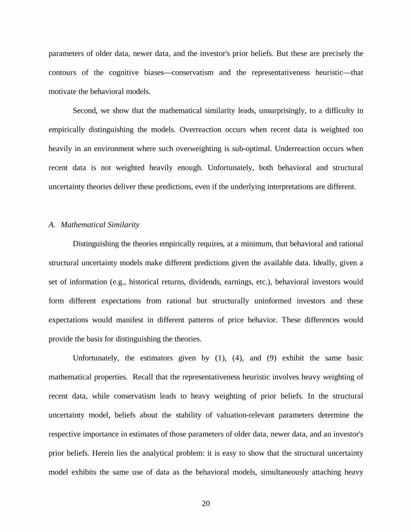
parameters of older data, newer data, and the investor's prior beliefs. But these are precisely the

contours of the cognitive biases— conservatism and the representativeness heuristic— that

motivate the behavioral models.

Second, we show that the mathematical similarity leads, unsurprisingly, to a difficulty in

empirically distinguishing the models. Overreaction occurs when recent data is weighted too

heavily in an environment where such overweighting is sub-optimal. Underreaction occurs when

recent data is not weighted heavily enough. Unfortunately, both behavioral and structural

uncertainty theories deliver these predictions, even if the underlying interpretations are different.

A. Mathematical Similarity

Distinguishing the theories empirically requires, at a minimum, that behavioral and rational

structural uncertainty models make different predictions given the available data. Ideally, given a

set of information (e.g., historical returns, dividends, earnings, etc.), behavioral investors would

form different expectations from rational but structurally uninformed investors and these

expectations would manifest in different patterns of price behavior. These differences would

provide the basis for distinguishing the theories.

Unfortunately, the estimators given by (1), (4), and (9) exhibit the same basic

mathematical properties. Recall that the representativeness heuristic involves heavy weighting of

recent data, while conservatism leads to heavy weighting of prior beliefs. In the structural

uncertainty model, beliefs about the stability of valuation-relevant parameters determine the

respective importance in estimates of those parameters of older data, newer data, and an investor's

prior beliefs. Herein lies the analytical problem: it is easy to show that the structural uncertainty

model exhibits the same use of data as the behavioral models, simultaneously attaching heavy

21

weight to prior beliefs (conservatism) and heavy weight to recent data (the representativeness

heuristic). More formally consider the following definitions:

Definition 1: The Bayesian change-point estimator (used to model thestructural uncertainty investor) displays conservatism when it attachesgreater weight to the prior beliefs than the stable Bayesian estimator.

Definition 2: The Bayesian change-point estimator displays therepresentativeness heuristic when recent data receive greater weight thanpast data.

Proposition: The estimator in (9) exhibits both conservatism and therepresentativeness heuristic.

Proof: See Appendix 3.

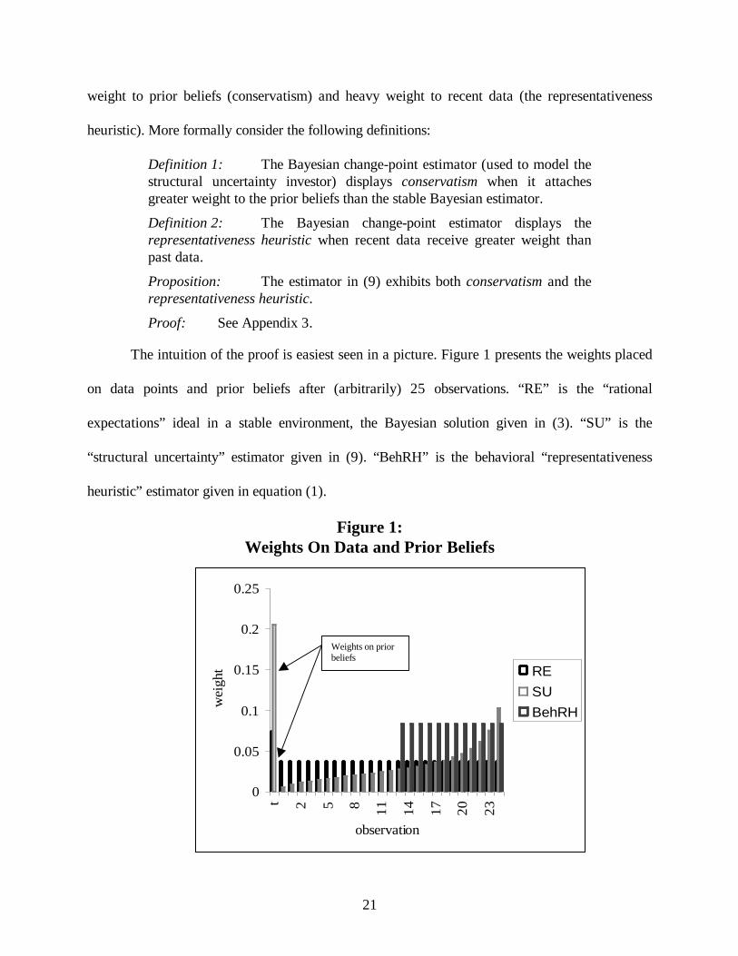
The intuition of the proof is easiest seen in a picture. Figure 1 presents the weights placed

on data points and prior beliefs after (arbitrarily) 25 observations. “RE” is the “rational

expectations” ideal in a stable environment, the Bayesian solution given in (3). “SU” is the

“structural uncertainty” estimator given in (9). “BehRH” is the behavioral “representativeness

heuristic” estimator given in equation (1).

Figure 1:Weights On Data and Prior Beliefs

0

0.05

0.1

0.15

0.2

0.25

t 2 5 8 11 14 17 20 23

observation

wei

ght RE

SUBehRH

Weights on priorbeliefs

22

The behavioral investor with conservatism attaches more weight to the prior than

warranted. That is, more than shown by the dark bar weighting prior beliefs (since the dark bar is

the rational expectations bar in a stable environment). The behavioral investor using the

representativeness heuristic applies all weight to recent data, much more than the dark bars

(which are all equal, since each data point is equally valuable to the Bayesian investor with

complete structural knowledge).

Now consider the problem of the investor with rational structural uncertainty. He must

consider 25 possibilities. First, he must consider the possibility that that there was no change in

the underlying valuation-relevant parameter. In that case, all the data is relevant. The investor

calculates an estimate, assuming the parameter was stable over those 25 observations (as in (3)).

That possibility gets weighted by the posterior probability that there was no change. But the

investor must next consider the possibility that the valuation-relevant parameter changed after the

first observation. If it did change, then only data points 2 through 25 are relevant; data point 1,

since it was generated by the old parameter value, is irrelevant. The investor calculates an

estimate, assuming the parameter was stable over those last 24 observations (again, as in (3)).

That possibility gets weighted by the posterior probability that there was a change after the first

observation. This continues all the way until the possibility that the valuation-relevant parameter

just changed last period, in which case there was only a single data point from that parameter,

observation 25. The investor calculates an estimate, assuming the parameter was stable over only

that last observation (again, as in (3)). That possibility gets weighted accordingly.

Note that this leads to two effects. First, later data receive much more weight in the final

estimate. Consider the last data point. It gets included in every calculation. But the first data point

gets included only in the first possibility (the “no change” scenario). This leads to the declining

23

pattern in Figure 1. But this is just greater weight on recent data, consistent with the

representativeness heuristic. Second, consider what happens to the weight on the prior. Note from

(3) that as the number of observations decreases, the weight on the prior increases. But as each

scenario is played out as above, the number of data points in each scenario is decreasing (first 25,

then 24, … ., all the way to 1). Thus, the weight on the prior is necessarily higher than the weight

given by (3). But higher weight on the prior is just like conservatism.

Thus, at a basic level the theories are hardly distinguishable, if at all, based on their use of

data and prior beliefs. Investors placing heavy weight on prior beliefs may be acting irrationally

and displaying conservatism, but they also may be placing more weight on prior beliefs in the

(rational) belief that the underlying parameters are unstable, rendering old data irrelevant and thus

lowering the available sample size. With a lower sample size, heavy weight on prior beliefs is

optimal. Alternatively, investors placing heavy weight on recent data may be acting irrationally

and displaying the representativeness heuristic, but they also may be placing more weight on

recent data in the (rational) belief that the underlying parameters are unstable, rendering the older

data less relevant to their estimates. With unstable parameters, recent data is generally the most

relevant data.

B. The Simple Models and Prior Empirical Evidence

As the mathematical results suggest, distinguishing the theories empirically is difficult.

This is further complicated by the fact that the empirical environments lend themselves to both

behavioral and rational structural uncertainty interpretations. Consider first the empirical results

on overreaction. In each case, most of the evidence suggests that investors sometimes (but not

always) attach too much weight to recently good or bad performance and over- or undervalue

24

stocks accordingly. That the evidence is consistent with the major behavioral hypothesis that

investors fall prey to the representativeness heuristic seems clear, essentially by definition. But the

nature of these tests also makes them consistent with the structural uncertainty model presented

above. The portfolio formation strategies in overreaction studies tend to sort on proxies for

stability. Thus, they may tend to select many stocks priced by investors whose concern with

potential instability was (ex post) too severe. Consider the superiority of value stock investment

strategies over growth stock investment strategies documented by Lakonishok, Shleifer, and

Vishny (1994). Value stocks that outperform growth stocks are consistent poor performers, in

terms of earnings, cash flow, and sales growth, both before and after portfolio formation. Growth

stocks are consistent good performers, in terms of earnings, cash flow, and sales growth, both

before and after portfolio formation. This portfolio formation strategy (and the similar returns-

based approach of DeBondt and Thaler (1985)) may identify value stocks that are priced too low

due to the overweighting of especially bad recent performance, and growth stocks that are priced

too high due to overweighting of especially good recent performance. When future performance

of these value stocks is not especially bad, their prices rise.

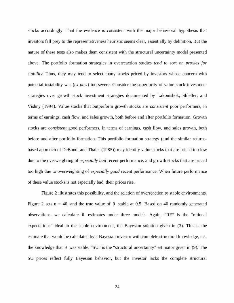
Figure 2 illustrates this possibility, and the relation of overreaction to stable environments.

Figure 2 sets n = 40, and the true value of θ stable at 0.5. Based on 40 randomly generated

observations, we calculate θ estimates under three models. Again, “RE” is the “rational

expectations” ideal in the stable environment, the Bayesian solution given in (3). This is the

estimate that would be calculated by a Bayesian investor with complete structural knowledge, i.e.,

the knowledge that θ was stable. “SU” is the “structural uncertainty” estimator given in (9). The

SU prices reflect fully Bayesian behavior, but the investor lacks the complete structural

25

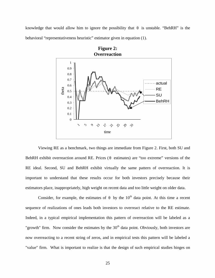
knowledge that would allow him to ignore the possibility that θ is unstable. “BehRH” is the

behavioral “representativeness heuristic” estimator given in equation (1).

Figure 2:Overreaction

0

0.1

0.2

0.3

0.4

0.5

0.6

0.7

0.8

0.9

1

1 5 9 13 17 21 25 29 33

time

thet

a

actualRESUBehRH

Viewing RE as a benchmark, two things are immediate from Figure 2. First, both SU and

BehRH exhibit overreaction around RE. Prices (θ estimates) are “too extreme” versions of the

RE ideal. Second, SU and BehRH exhibit virtually the same pattern of overreaction. It is

important to understand that these results occur for both investors precisely because their

estimators place, inappropriately, high weight on recent data and too little weight on older data.

Consider, for example, the estimates of θ by the 10th data point. At this time a recent

sequence of realizations of ones leads both investors to overreact relative to the RE estimate.

Indeed, in a typical empirical implementation this pattern of overreaction will be labeled as a

"growth" firm. Now consider the estimates by the 30th data point. Obviously, both investors are

now overreacting to a recent string of zeros, and in empirical tests this pattern will be labeled a

"value" firm. What is important to realize is that the design of such empirical studies hinges on

26

selecting growth firms whose fundamentals have been consistently high (high θ firms), and

comparison of their average return with the average return on value firms whose performance has

been lackluster in the past (low θ firms).

Next, consider underreaction. The presence of underreaction is consistent with

conservatism, as investors overweight prior beliefs and fail to take proper account of the new

evidence (again, essentially by definition). But underreaction is also consistent with the presence

of investors who are unsure whether the change in fact occurred, and continued to use too much

data from an earlier environment. And, perhaps not surprisingly, the portfolio formation strategies

in underreaction studies have sorted on good proxies for instability. Consider the superiority of

momentum strategies documented by Chan, Jegadeesh, and Lakonishok (1996). They sort firms

based on standardized unexpected earnings, extreme recent returns, and changes in analysts'

forecasts. On each measure, winners continue to be winners in the immediate future, while losers

continue to be losers. It is at least plausible that such shocks reflect fundamental change in some

underlying valuation-relevant parameter. The authors find little evidence of price reversals. The

drift to new price levels is permanent, consistent with the existence of an actual change in a

valuation-relevant parameter that investors recognized only slowly.

This is consistent with both behavioral and structural uncertainty models. Figure 3 also

sets n = 40, but now θA = 0.75 generates all observations from 1,… ,20, while θB = 0.25 generates

the remaining observations from 21,… ,40. Based on 40 randomly generated observations, we

again calculate θ estimates under three models. “RE” is again the “rational expectations” ideal,

this time in the unstable environment. This means simply that the RE investor would use the

Bayesian solution given in (3) on the data through time 20, and would then discard the data

1,… 20 and begin using (3) on the data 21,… 40. In this way, the Bayesian RE investor would not

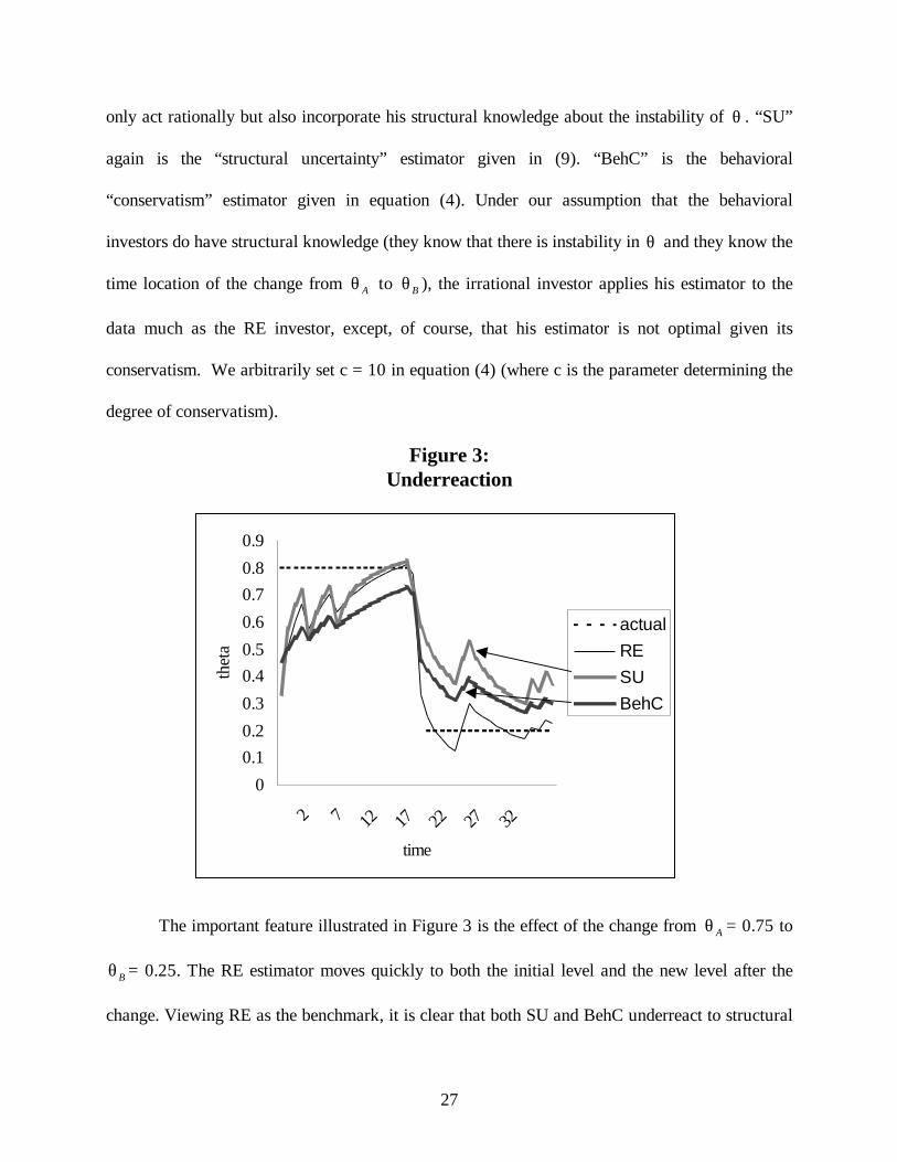
27

only act rationally but also incorporate his structural knowledge about the instability of θ . “SU”

again is the “structural uncertainty” estimator given in (9). “BehC” is the behavioral

“conservatism” estimator given in equation (4). Under our assumption that the behavioral

investors do have structural knowledge (they know that there is instability in θ and they know the

time location of the change from θA to θB ), the irrational investor applies his estimator to the

data much as the RE investor, except, of course, that his estimator is not optimal given its

conservatism. We arbitrarily set c = 10 in equation (4) (where c is the parameter determining the

degree of conservatism).

Figure 3:Underreaction

The important feature illustrated in Figure 3 is the effect of the change from θA = 0.75 to

θB = 0.25. The RE estimator moves quickly to both the initial level and the new level after the

change. Viewing RE as the benchmark, it is clear that both SU and BehC underreact to structural

00.10.20.30.40.50.60.70.80.9

2 7 12 17 22 27 32

time

thet

a

actualRESUBehC

28

changes. The reasons are related but slightly different. The behavioral investor is attaching far too

much weight to his prior beliefs and failing to extract enough information about the new

environment. This despite the fact that the behavioral investor “knows” the right data to use.

Consider observation 25, the fifth observation generated by new parameter. The optimal weight

on the prior is, from (3), 0.29 (=2/7). The weight placed on the prior by the conservative investor

is 0.67 (=10/15). At this point, the SU investor is not necessarily overweighting prior beliefs (his

weight is about 20%) but this is not a general feature of the model. The SU investor’s prior

weighting will in general be too high or too low, depending on the occurrence and location of

actual parameter change in the data. More importantly for the SU investor, his inability to know

exactly where the change occurred leaves him using substantial amounts of data from the old

(θA ) environment. His estimates tend to drift rather slowly, as more and more data from the new

environment enters his estimates.

Once again, it is important to note that Figure 3 illustrates what happens when actual

instability exists. The empirical studies mentioned above are geared to detect and select events in

which an abrupt structural change has actually occurred. Our analysis indicates that the resulting

empirical evidence of return continuations is equally consistent with both behavioral and structural

uncertainty interpretations.

III. Normative DifferencesWe have shown that certain behavioral and structural uncertainty models can explain the

same financial anomalies, and stressed how similarity of their mathematical structures and the

nature or empirical environments might make it hard to distinguish them. In this section, however,

we focus on a fact that can be hidden by these similarities: behavioral and structural uncertainty

29

theories have different normative implications. The normative differences hinge on the crucial

distinction between behavioral and structural uncertainty approaches: investors in the behavioral

approaches are setting sub-optimal prices, while investors in the structural uncertainty approach

are perfectly rational given available information. The potential differences here are visible on the

face of current research. To illustrate, consider the differences between Barsky and DeLong

(1993) and Lakonishok, Shleifer, and Vishny (1994). The former study of stock market

fluctuations acknowledges that prices move more than future dividends, but there is no hint that

the authors think they could have done better than the market in dealing with the uncertainty

about dividend growth. The latter study of the value-growth anomaly reads as a virtual how-to

manual in exploiting investor irrationality. Indeed, the authors have put their money where their

mouths were: LSV Asset Management now has billions of dollars under management investing

along the lines suggested by the paper.

Consider just three examples where normative differences are almost sure to arise: cost of

capital estimation, money management, and capital market regulatory policy. First, “true” costs of

capital may be hard to infer from market prices in a behavioral theory [Stein (1996), Haugen

(1999)], while adjustments to infer costs of capital in structural uncertainty models may be much

easier [see, for example, Mayfield (1999)].15 Second, money management practices are sure to be

effected by the respective theories. Risk arbitrage resources in a behavioral world focus largely on

betting against investor irrationality; in a structural uncertainty world, resources focus on better

identifying structural breaks and processes.

15 It is common, for example, to estimate the market premium on the basis of 10 or 20 years of data, rather thanthe full series of market and treasury bill/bond returns. Such procedures reflect a concern that the underlyingmarket premium may have changed over time [Pastor and Stambaugh (1998)]. For one approach to estimating themarket risk premium in light of structural uncertainty, see Mayfield (1999).

30

Finally, capital market regulatory policy, such as the regulation of securities markets and

issuance, will surely be influenced by the dominant approach. At stake here is the degree of

government intervention justified by the behavior of financial markets, e.g., in securities

regulation, retirement income security and private social security, etc. Structural uncertainty

models, following the assumption of investor rationality, leave little role for government

intervention beyond providing basic information, and perhaps even that role is questionable [see

Easterbrook and Fischel (1992; Ch. 11)]. Matters are far different when investors might be

irrational. As Jolls, Sunstein, and Thaler (1998) remark in their recent paper on behavioral law

and economics:

In its normative orientation, conventional law and economics is often stronglyantipaternalistic. The idea of “consumer sovereignty” plays a large role; citizens,assuming they have reasonable access to relevant information, are thought to bethe best judges of what will promote their own welfare. Yet many of the instancesof bounded rationality discussed above call this idea into question…

However, as Jolls, Sunstein, and Thaler (1998) stress, the presence of cognitive and motivational

biases provides a strong basis for "anti-antipaternalism," that is, "a skepticism about

antipaternalism, but not an affirmative defense of paternalism"16 mostly because it is unclear that

regulators and lawmakers could do better.

Further, if irrationality and structural uncertainty are highly correlated (see below), then it

may be difficult for even a rational regulator to provide solutions to apparently irrational capital

market activity. Ex ante, it may be impossible for the structurally uncertain regulator to be sure

enough of his view that regulation is justified. Ex post, it may be impossible for the structurally

uncertain regulator to determine whether events like stock market crashes reflected irrationality

requiring government intervention, or rational structural uncertainty. One need look no farther

16 p. 1541.

31

than the history of the 1929 stock market crash and the ensuing (and enduring) system of U.S.

securities regulation (in particular, the Securities Act of 1933, and the Securities Exchange Act of

1934) for a case study in this problem.

IV. The Coexistence of Behavioral And Rational TheoriesMost of our analysis so far has focused on the differences between behavioral and

structural uncertainty models as if they must exist independently. In fact, however, this view

overlooks the present connections between the two theories. These connections are apparent,

though not emphasized, in the emerging “limits of arbitrage” literature. That literature emerged

because of the so-called “arbitrage objection” to behavioral finance: the claim that competitive

arbitrage will drive to zero any mispricing caused by behavioral traders' bad investment strategies.

While this objection sounds nearly irrefutable, recent theoretical and empirical analyses of

arbitrage have weakened its force somewhat, and allowed behavioral theories to proceed with less

worry [Shleifer and Vishny (1997), Pontiff (1996)]. Consider Shleifer and Vishny (1997). They

point out that arbitrageurs typically speculate with other people's money and those people tend to

withdraw funds after poor performance. Since an arbitrageur's poor performance may reflect only

the short-term deepening of mispricing, the prevalence of performance-based arbitrage may leave

the most severe episodes of mispricing unmitigated. Arguments like these suggest that

irrationality-induced anomalies might survive.

What is often overlooked, however, is that behavioral finance has become intimately

connected with the structural uncertainty approach in these appeals to the limits of arbitrage.

Consider again the Shleifer and Vishny (1997) model of performance-based arbitrage. Why

investors in arbitrage funds should withdraw funds from arbitrageurs after bad performance is

32

somewhat puzzling, given the obvious possibility that mispricing from which they hope to profit

may simply have deepened. Interestingly, Shleifer and Vishny (1997), though clearly focused on

the survival of irrationality-induced anomalies, appeal to rational structural uncertainty on the

part of investors who provide capital to arbitrageurs:

Both arbitrageurs and their investors are fully rational… We assume that investorshave no information about the structure of the model determining assetprices… Implicitly we are assuming that the underlying structural model issufficiently nonstationary and high dimensional that investors [who providearbitrageurs with funds] are unable to infer the underlying structure of the modelfrom past returns data… Under these informational assumptions, individualarbitrageurs who experience relatively poor returns in a given period lose marketshare to those with better returns.”17

In other words, the key to the limits of arbitrage in Shleifer and Vishny (1997) is the

existence of rational structural uncertainty on the part of their investors, not cognitive biases. As a

modeling strategy, of course, this is unnecessary. One could write a limits of arbitrage theory

without rational structural uncertainty. For example, the Shleifer and Vishny (1997) model might

have assumed that the arbitrageur raised money from irrational investors whose beliefs are

correlated with the noise traders against whom the arbitrageurs speculate. But such a theory

would have been less convincing. Assuming that all investors are irrational but the capital-poor

arbitrageur is somehow less convincing than assuming that there are some rational investors with

capital who nevertheless fail to exploit every instance of mispricing. But if irrationality-induced

anomalies survive because these rational actors with money do not bet fully against them, there

must be a reason. Rational structural uncertainty provides such a reason, and Shleifer and Vishny

(1997) rest their model upon it.

This suggests that the coexistence of behavioral and rational structural uncertainty theories

could help researchers understand where each is likely to be important or dominant. First, if there

33

are rational arbitrageurs with capital, then rational structural uncertainty is virtually a necessary

condition for the presence of an irrationality-induced anomaly. Behavioral theories that posit the

survival of irrationality-induced anomalies could state explicitly the sources of rational structural

uncertainty that will limit arbitrage. Second, future studies of arbitrage will likely benefit from an

explicit acknowledgment of the tension between investor irrationality and rational structural

uncertainty. On the one hand, more investor irrationality creates more opportunity for arbitrage

profits. On the other hand, investor irrationality and structural uncertainty may be highly

correlated. The optimal allocation of arbitrage resources requires a trade-off, and anecdotal

evidence suggests that arbitrage resources might be allocated roughly accordingly [see Shleifer

and Vishny (1997)].

V. A More Agnostic Approach to Finance and Structural Uncertainty?Our comparative analysis has shown that the basic assumption of structural uncertainty

has considerable power in generating interesting usage of prior beliefs and data. These models are

able to generate the types of behaviors that have otherwise required appeal to experimental

results. To many economists, resting assumptions about investor behavior on experimental results

devoid of either axiomatic foundation or economic context is very unappealing. For them, an

approach that delivers the theoretically useful behaviors (like overweighting recent data and prior

beliefs) within a Bayesian model allows adherence to the rational approach within which many are

more comfortable.

One must ask, however, whether it is necessary or desirable to adhere so strongly to the

“rational” characterization of this approach. It is easy to see that what drives the explanatory

17 pp. 38, 40 (emphasis added).

34

power of these models is not the labeling of “rational” or “behavioral” but the particular patterns

of data use that result. The appeal of the structural uncertainty approach is that it provides an

economic context for deriving these effects. Focusing on the “rationality” of the approach given

its Bayesian foundation may be more rhetorical than real [McCloskey (1983)]. After all, these

models work in generating financial anomalies only because these “rational” beliefs are

nevertheless mistaken— that is, the resulting subjective distributions do not line up with objective

distributions governing the economy.

Consider the recent model of Barberis, Shleifer, and Vishny (1998). The authors interpret

their model as capturing both the representativeness heuristic and conservatism, and there is no

doubt that they intend for their representative investor to be interpreted in a behavioral sense. But

(as they acknowledge) one fact about their model is striking: it is fully Bayesian so that the

model’s mathematical structure is, in a formal sense, fully consistent with rational information

processing. Their results are driven by the fact that their representative investor holds the prior

belief that the true model for earnings is impossible (not in the support of his prior over models).

In an essentially isomorphic approach, however, Nyarko (1991) examined the monopolist's

problem of learning a demand curve when the true parameters of the demand curve lie outside the

support of his prior distribution. He shows that— similar to the Barberis, Shleifer, and Vishny

(1998) result— the monopolist would cycle indefinitely between two erroneous models that come

closest to the true model, which by assumption he can never learn. Nyarko (1991) adopts a

completely rational interpretation of his model. What is important in both approaches— in terms

of delivering interesting testable predictions of economic behavior— is the structural uncertainty,

not the philosophical characterization. Despite occasional assertions to the contrary, we see no

35

reason to rest the validity of the structural uncertainty approach on the degree to which it can be

characterized as rational.18

Instead, we believe that an important lesson of the comparative analysis is that there is

much to recommend what might be called a more “agnostic” structural uncertainty framework.

Such an approach may retain the modeling structure offered by Bayesian and other methods. At

the same time, these models are capable of some degree of “hard-wiring” that allows them to

model a wide-range of beliefs and expectations formation, including those that result in behaviors

consistent with experimental biases. Such an approach would essentially divorce itself from

largely philosophical characterizations, in recognition that “[t]he rationality of a behavior is

irrelevant to its cause or explanation.” [Cosmides and Tooby (1994, p. 327)]. This is not to say

that the assumptions of the structural uncertainty model are without empirical support. Aside

from the uncontroversial plausibility of the structural uncertainty approach to most economists,

there are reasons to believe that humans may be adapted to a concern with structural uncertainty

that does not always serve them well in artificial laboratory settings. They may indeed not be so

bad as experiments might make them look, while not being so rational that they can put aside their

adapted beliefs when logic would dictate doing so (for example, when facing an obviously

stationary bookbag and poker chip experiment) [see Winkler and Murphy (1973)].

18 For example, in one of the most intricate and thought-provoking approaches to rational structural uncertainty,Kurz (1994) hinges the validity of his theory on its rationality: “The validity of our approach does not depend onthe existence of a conclusive proof for non-stationarity. It does, however, hinge on the fact that we do not have aconclusive theoretical reasoning to compel a rational agent to believe that his environment is stationary. Wetherefore only require that an economic agent not be declared irrational if he takes the view that the economicprocess at hand may be non-stationary.” Since his predictions do not depend on the characterization of the agent asrational or not, we are unsure why the “validity” of the approach depends on it.

36

There may be evolutionary psychology explanations for concern with structural

uncertainty, while modern capital market price determination problems differ radically from those

that shaped its evolution [Gigerenzer (1991), Cosmides and Tooby (1994, 1996)]. Consider the

following example, from Gigerenzer (1991), which highlights how the structure of the

environment impacts probabilistic reasoning. The example involves two thought experiments. In

the first experiment, you consider purchasing a new car and need to choose between a Volvo and

a Saab. Your only choice criterion is the car's life expectancy. The Volvo has a superior track

record backed by several hundred consumer reports. Just yesterday however, your neighbor told

you that his Volvo broke down. Which car do you decide to buy?

In the second thought experiment you live in the jungle. Your child needs to cross a river

and you need to decide whether the crossing will be done by swimming or by climbing trees. The

choice criterion, again, is life expectancy. You are told that over the last 100 years only once did a

crocodile kill a child while several dozen children died by falling from trees. Just yesterday your

neighbor told you that his child was eaten by a crocodile. Where do you send your child?

Gigerenzer argues that most prospective buyers would choose to purchase the Volvo.

However, in the second experiment, he argues that parents will suspect that crossing the river by

swimming is now much riskier:

Why do we have different intuitions for the Volvo and the crocodile problem? Inthe Volvo problem, the prospective buyer may assume that the Volvo world isstable, and that the important event (good or bad Volvo) can be considered as anindependent random drawing from the same reference class. In the crocodileproblem, the parents may assume that the river world has changed, and that theimportant event (being eaten or not) can no longer be considered as anindependent random drawing from the same reference class. Updating "old" baserates may be fatal for the child. … If so, the content of problems is of centralimportance for understanding judgment -- it embodies implicit knowledge aboutthe structure of the environment.

37

Whatever the philosophy, it is clear that a structural uncertainty approach has considerable

explanatory power. Given the flexibility to “hard-wire” certain beliefs, it can capture important

psychological behaviors, yet retain the modeling capability of traditional methods. We have

already shown how this approach can capture behaviors associated with the representativeness

heuristic and conservatism, generating price overreaction and underreaction. In the next section of

the paper, we provide one more illustration of this approach. We show how yet another cognitive

bias— overconfidence— can also arise from structural uncertainty.

VI. Illustration: Deriving Overconfidence From Structural UncertaintyOverconfidence is a well-known bias that— like the representativeness heuristic and

conservatism— has enjoyed application in behavioral finance. Overconfidence is the belief that the

precision of one’s information or beliefs is greater than actual. Overconfident individuals

underestimate the variance surrounding their beliefs. Put differently, overconfident individuals are

too sure of themselves. Overconfidence has been applied in the work of Daniel, Hirshleifer, and

Subramanyam (1998) and O’Dean (1998) by assuming that investors arrive at variance estimates

that are too low.

Overconfidence arises in a structural uncertainty framework when an investor (or trader,

or manager) believes that some quantity of interest may be changing through time. Consider, for

example, an investor who is estimating the performance of an investment strategy by looking at

the mean and variance of its returns. He receives return data through time. Now consider two

types of investors. Both believe that the unknown variance does not change over time. However,

the first type of investor believes that the unknown mean return of the investment strategy may

have changed over the period, while the second type of investor believes that the unknown mean

38

return to the strategy is stable through time. We now show that the structural uncertainty of the

first investor will lead him to be too sure of his estimate of the mean return to the strategy relative

to the second investor, whenever the unknown mean return is in fact stable. The intuition of the

result, which we prove below, emerges from the following two observations. First, the investor

who holds the correct beliefs in stability derives his posterior beliefs regarding the unknown

variance by calculating a sum of squares measure about his posterior estimate of the unknown

mean. Second, the investor, who is concerned with instability, calculates his sum of squares about

more than one sample mean as he allows for a possible change. Consequently, this additional

“degree of freedom” results in posterior beliefs regarding the variance which are too low.

To formally address overconfidence we need to shift from the one-parameter, beta-

binomial change-point problem, to the case were the data is normally distributed (obviously, the

intuition from our previous results carries over). Let there be n observations on the investment

strategy’s return, denoted by nxx ,,1 K . The investor does not know the mean or the variance

generating the data. For an investor who believes that there may be a change-point, denote

( )BA µµ , as the mean before and after the possible change respectively. Let the precision (inverse

of the variance) be denoted by τ , also unknown to the investor. The joint likelihood, as in Smith

(1975), is proportional to:

( ) ( ) ( ) ( )

∑ −+∑ −⋅−⋅∝

+==

n

riBi

r

iAi

n

BA xxrnxxl1

2

1

22

21

exp,,,,,1 µµτττµµK (10)

We employ diffuse prior beliefs on the model parameters, as in Smith (1975),

( ) τµµττµµ dddp BABA1,, −∝ . The prior beliefs on the possible change points { }nr ,,1K∈ are

diffuse as in Section I. The posterior probability of a change at point r, denoted )(rpn is

39

obtained by integrating the likelihood function with respect to the unknown mean and precision

parameters and is proportional to:

( ) ( ){ } ( ) ( )

( ) ( )( )

nrxxnnrp

nrxxxxrnrrp

nn

inin

nn

rirni

r

irin

=

−⋅∝=

−=∀

−+−⋅−⋅∝

−−

=

−

−−

+=−

=

−

∑

∑∑1

21

1

221

12

1

2

1

221

1,,1K (11)

The constant of proportionality is ( ) ,1

1

−

=

∑

n

rn rp and ∑

=

− ⋅=r

iir xrx

1

1 ,

( ) ∑+=

−− ⋅−=

n

riirn xrnx

1

1 , and .1

1 ∑=

− ⋅=n

iin xnx

To show that the estimates of the investor concerned with instability will be too precise

relative to the investor not concerned, we derive the posterior distribution of the precision

parameter ( )τnp . First, note that the posterior distribution of τ conditioned on a break occurring

at ( )nrr ≤≤1 is in the form of a Gamma distribution:

( ) ( ) ( )

( ) ( ) ( ) nrxxnrp

nrxxxxrp

n

ini

n

n

n

rirni

r

iri

n

n

=

−⋅−⋅∝=

−=∀

−+−⋅−⋅∝

∑

∑∑

=

−

+=−

=

−

1

2121

1

2

1

222

21

exp

1,,121

exp

τττ

τττ K

(12)

Second, the posterior distribution of the precision parameter ( )τnp , which integrates over

the uncertainty regarding the possible change point, is just the weighted average of these

conditional distributions using the posterior probabilities of a change ( )rpn as weights. The

posterior mean of ( )τnp , SUτ̂ , is given by the following expression

40

( ) ( )

( ) ( )( ) ( )

( )∑∑

∑∑=

−

=

+=−

=−

=⋅−+

−+−

⋅−= n

ini

nn

rn

rirni

r

iri

nSU

xx

nrpn

xxxx

rpn

1

2

1

1

1

2

1

2

12τ̂ (13)

Note however, that in the case of correct knowledge of stability, the posterior distribution

is in the Gamma form as well:

( ) ( ) ( )

−⋅−⋅∝ ∑

=

− n

ini

n

n xxp1

2121

21

exp τττ (14)

and its posterior mean, denoted by REτ̂ , is given by

( )( )∑

=−

−= n

ini

RE

xx

n

1

2

1τ̂ (15)

It is clear from equations (13) and (15) that SUτ̂ , the precision of the structurally

uncertain investor, must be higher than the posterior mean precision of the investor who believes

in complete stability, REτ̂ . This follows from the following inequality:

( ) ( ) ( )∑∑∑=+=

−=

−≤−+−n

ini

n

rirni

r

iri xxxxxx

1

2

1

2

1

2

Which holds strictly whenever the sub-sample means ( )rnr xx − are not equal to the overall sample

mean 1,,1, −=∀ nrxn K . This inequality captures much of the intuition which we outlined

earlier. The investor who correctly believes in stability calculates his measure of precision relative

to the overall sample mean. However, an investor concerned with a possible change-point will

derive his measure of precision relative to what he considers to be the changing sample means

which necessarily lead to a lower overall sum of squares and therefore to a higher precision.

It is therefore possible to build theories of overconfident behavior that rest on beliefs

about changing means. Reconsider, for example, the Shleifer and Vishny (1997) model of

performance-based arbitrage and the behavior of outside investors who provide capital to

41

arbitrageurs. If these investors entertain the possibility that arbitrageurs' abilities may be changing

over time whereas in fact they are unchanging then our analysis suggests that such beliefs about

ability will be excessively certain. Moreover, our previous analysis regarding the incidence of

overreaction in stable environments suggests that the investors' tendency to overreact, that is,

conclude that the arbitrageur's ability is higher/lower than it actually is, will coincide with

overconfidence. Consequently, a series of negative returns will lead outside investors to believe

that ability is lower than it actually is and, at the same time, to be overconfident regarding the

precision of these beliefs. This is likely to lead to even larger capital withdrawals from the

arbitrageur and limit his ability to bid against perceived mispricing.19

As with our earlier results, our point is not that structural uncertainty necessarily causes

overconfidence. So far as we know not even psychologists have arrived at a unifying theory of

overconfidence [see Griffin and Varey (1996), Griffin and Buehler (1999), and Brenner, Koehler,

Liberman, and Tversky (1996) and the references therein]. The structural uncertainty framework

however provides an economic context in which such behavior is derived rather than assumed.

Interestingly, our prediction that overconfidence is likely to coincide with overreaction

(representativeness heuristic) has been advanced in the psychology literature [Griffin and Tversky

(1992)]. Griffin and Tversky suggest that confidence is a function of the extremeness of the

evidence and its credence. Overconfidence arises when subjects focus on the extremeness of the

evidence with insufficient regard to credence. Underconfidence is hypothesized to occur when the

extremeness of the hypothesis is low and its credence is high. Griffin and Tversky therefore

propose that overconfidence will occur when base rates are low (representativeness) while

19 The tendency of overreaction to coincide with overconfidence in such a stable environment could also bepotentially applied to model market crashes and excess volatility as investors react abruptly to a string of eithergood or bad asset performance.

42

underconfidence will occur when base rates are high (conservatism), similar to the predictions

made by the structural uncertainty model.

VII. Conclusion

We compare two competing theories of financial anomalies: (1) “behavioral” theories

relying on investor irrationality; and (2) rational “structural uncertainty” theories relying on

investor uncertainty about the structure of the economic environment. Each relaxes the traditional

rational expectations model differently. We illustrate both sets of theories in simple models

generating two financial anomalies: overreaction and underreaction. We use the well-known

cognitive biases of “conservatism” and the “representativeness heuristic” to motivate our

behavioral models. Both are deviations from optimal Bayesian judgment that have enjoyed

application in behavioral finance. In our rational structural uncertainty approach, we model a

Bayesian (i.e., rational) investor with uncertainty about the stability of the valuation-relevant

parameter.

We next ask whether these theories can be distinguished empirically. It is extremely

difficult to distinguish these theories empirically because both share striking mathematical and

predictive similarities. The predictive similarity of the two theories is troubling because the

theories have radically different normative consequences. Perhaps most importantly, implications

for capital market regulatory policy differ under each approach. It much easier to make a case for

paternalistic governmental intervention under a behavioral view where traders make mental errors

than under a structural uncertainty approach where traders are doing their rational best.

In some cases, the theories coexist. It is difficult to justify the survival of irrationality-

induced anomalies without assuming certain “limits of arbitrage” that prevent rational investors

43

from exploiting and correcting irrational prices. Shleifer and Vishny (1997) rest such a model of

limited arbitrage on rational structural uncertainty. Both theoretically and in the real world,

investor irrationality and rational structural uncertainty may be highly correlated.

We explore the possibility that choosing between the theories is not the answer at all,

however. Given the mathematical and predictive similarities of the theories, and the resulting

inability to distinguish them empirically, it is easy to make a case for shifting away from the

behavioral-rational debate, and toward greater focus on investor concern with structural

uncertainty, whether perfectly rational or not. The last sections of our paper focus on this

approach. In related work, we further extend the structural uncertainty approach in an attempt to

model IPO long-term performance. We focus on Loughran and Ritter's (1995) claim that

investors are irrationally optimistic about the future prospects of such firms. We show that a

structural uncertainty approach, similar to the one presented in this paper, can be implemented to

explain this phenomenon. Specifically, we show how a structurally uncertain investor's prior

beliefs on tail events such as probabilities of a "big winner" can be modeled with a simple

Bayesian mixture approach. This allows us to study directly the relationship between such prior

beliefs and posterior beliefs regarding mispricing. Finally, in Appendix 4, we show the consistency

of a rational structural uncertainty theory with the recent long horizon event study empirical

evidence.

One area that we have not explored is “learning.” While a full treatment of learning

remains for future work, we can say two things here. First, in the simple models of our earlier

work, learning is possible, but this is more an artifact of our modeling choices than a realistic

representation of likely behavior. Learning in experiments requires immediate outcomes and clear

feedback. Financial markets tend to present neither; outcomes are delayed and feedback is noisy.

44

Learning from experience is unlikely in such circumstances [see Brehmer (1980)]. Second, it has

long been clear that rational expectations equilibria will not necessarily just “happen” even if

agents have the chance to learn their way to that equilibrium among others. [See, for example,

Blume and Easley (1982)]. Even in our rational change-point models, the introduction of multiple

change-points, while quickly introducing intractable modeling problems, would prevent learning in

most scenarios. Further, many of the events from which investors might learn (such as the cross-

section of IPO returns) are positively correlated, cutting down the effective number of data points

from which to learn. In any psychological approach, such as the one we advocate in the later

section of our paper, “learning … is not an explanation for anything, but is rather a phenomenon

that itself requires explanation.” [Tooby and Cosmides (1992)].

45

APPENDIX 1

From equation (5) it is clear that

p p pn nr d d r r( ) ( ,... , ) ( )∝ 1 0 (A1)

Given independent beta priors for θ θA B, , both parameterized to give the uniform distribution,

and a uniform prior for the possible change-points, it follows that:

( ) ( )

( )( ) ( )

( ) ( )( )

( )( ) ( )

( ) ( )( )

( )( )

( )( )( )

( )( )

(A2) ,

)(),...,()(),...,(0

1

00

1

0

n1

1rn1

1r1

n1

!1rn!Drn!D

!Drn!D!rn

!1r!Dr!D

!Dr!Dr!

n1

2rn1Drn1D

112

Drn

2r1Dr1D

112

Dr

rpdpddpdpddprp

rnrn

rnrn

rr

rr

rnrn

rn

rr

r

0BBBn1rAAAr1n

×+−

×+

=

×+−−−×

−−−×

+−×

−=

×+−Γ

+−−Γ+Γ×ΓΓ

Γ×

−×

+Γ+−Γ+Γ×

ΓΓΓ×

=

∝

−−

−−

−−

−

+∫∫ θθθθθθ

where Dr denotes the number of 1's in the first r data observations, and Dn-r denotes the number

of 1's in the last n - r data observations. ( )Γ . denotes the gamma function.

Appendix 2

The mean of the posterior distribution for θn is given by:

( ) ( ) ( ) ( )

( ) ( ) ( ) ( )

( ) ( ) ( ) ( )

( ) ( ) ( ) ( ) (A3) , pp

pp

pp

ˆ1

0

1

0

1

++

++

+−+

+−−=

++

++

+−−+

+−−−−−+

+

+−+

+−−+

+−+

+−−=

=+=

−

−

=

−−

−−

−

=

∑

∫∫∑

21

2n2

D2n

nn

21

2i)(n2

D2i)(n

i)(ni

21

2n2

D2n

nn

21

21))(n(n2

D21))(n(n

1)(nn1n...

21

22)(n2

D22)(n

2)(n2

21

21)(n2

D21)(n

1)(n1

ddnpnrprprp

nnin

1n

1in

nn1)(nnn

2nn1nn

BA

n

1rnAnnBnn θθθθθ

46

where Dn i− denotes the mean of the last n - i observations (all observations after the change-point

on which the mean is conditioned) and the ( )pn i are as defined in (7).

Appendix 3

This appendix proves the proposition presented in section III.

Proof: Proving that (9) is consistent with conservatism and the representativeness heuristic

requires showing that it gives both more weight to prior beliefs that than the estimator in (3) and

more weight to recent data than old data. It is easiest to prove first the result on heavy weighting

of the prior. Note from (3) that the weight on the prior is:

2

2n +

. (A4)

The weight on the prior in the estimator of equation (9) is:

( ) ( )p in i

p nnn

i

n

n=

−

∑ − +

+ +

1

1 22

22( )

. (A5)

The first term is the weight on the prior of each possible estimator of θB while the second term is

the weight on the prior in the estimator of θA . Proving that the estimator in (9) overweights prior

beliefs relative to (3) requires showing that:

( ) ( )22

22

221

1

np i

n ip n

nni

n

n+

< − +

+ +

=

−

∑ ( ). (A6)

That is, the proof requires showing that the total weight on the prior in the estimator in (3) is

smaller than the total weight in the prior in the estimator of (9). To see that this is true, note first

that ( ) ( )n n i+ > − +2 2 for i = 1,… ,n - 1. This implies that

( ) ( )2

22

2n n i+ < − + ∀ i=1,… ,n. (A7)

47

Since p ini

n

=∑ =

11( ) (being probabilities) and p in

i

n

=

−

∑ ≠1

1

0( ) (by (7), showing that each of the change

points has nonzero probability), this implies that

( ) ( ) ( )p in

p in i

p nnn

i

n

ni

n

n= =

−

∑ ∑+ < − +

+ +

1 1

122

22

22

( ) ( ) . (A8)

Since

( ) ( )p in nn

i

n

=∑ + = +1

22

22

( ) , (A9)

the proof for conservatism is complete.

To prove the result for the representativeness heuristic (heavy weighting of recent data),

consider equation (9):

( ) ( ) ( ) ( )$θn ni 1

n 1

n i n ni(n i)

(n i) 2D

2(n i) 2

12

nn

n 2D

2n 2

12

= −− + + − +

+ + + +

=

−

−∑ p p (A10)

The data enter the estimator through the sample means, Di . The proof involves showing that

recent data enters more of these sample means than old data, and receives more weight in the

estimator. Consider first the third term. This term captures the possibility in the investor's mind

that there was no change from θA to θB . Therefore, all n data points enter the sample mean, Dn ,

in that term. Each of the n data points receives weight:

( )p nn

nnn

12

+

(A11)

from the sample mean that enters that term. This weight is made up of three parts. First, the

posterior probability of the "no change" point r = n. Second, the term 1 n in the calculation of

the sample mean for n observations. Third, the weight on the sample mean when there are n

observations and a uniform prior.

48

A data point enters the other sample means Dn i− only if it occurs after the change-point i.

For example, if i = 2, the sample mean Dn − 2 includes only observations occurring after the second

observation (since, by definition, this means that θA generated the first two observations, then a

change occurred, and θB generated all remaining observations). Thus each data point

j n∈ { ,... , }2 (remembering that the only weight the first observation can receive is the weight if no

change occurred) also receives the sum of the weights associated with each sample mean that

includes that observation. For a given data point j, this weight is given by:

p kn k

n kn kn

k

j

( )( )

121

1

−

−− +

=

−

∑ (A12)

Consider, for example, observation 4. There are 3 terms in the sum of the weight on observation 4

conditional on some change (k=1 to 3). First, the change could have occurred at observation 1, in

which case observation 4 will enter into the sample mean constructed from all observations after

the first. Second, the change could have occurred at observation 2, in which case observation 4

will enter into the sample mean constructed from all observations after the second. Finally, the

change could have occurred at observation 3, in which case observation 4 will enter into the

sample mean constructed from all observations after the third. After that, however, the change

will take place at or after observation 4, so observation 4 cannot enter the calculation of the

sample mean.

Combining the weights that arise from change and no change, we get the weight placed on

observation j n∈ { ,... , }2 in the estimator:

( )p kn k

n kn k

p nn

nnn

k

j

n( )( )

12

121

1

−

−− +

+

+

=

−

∑ (A13)

49

This sum is increasing in j, while the weight on observation j=1 is simply ( )p nn

nnn

12

+

. This

completes the proof for the representativeness heuristic (heavy weighting of new data).

Appendix 4

In this Appendix we demonstrate the consistency of a rational structural uncertainty theory

of the type presented in section I.E with recent event study empirical evidence. While the

literature on event study "drifts" is large (see Appendix A in Daniel, Hirshleifer, and

Subrahmanyam (1998)), the pattern of pre-event, event-day, and post-event abnormal returns can

be stratified into four main cases depending on the sign of respective abnormal returns.

Pre-Event Event-Day Post-EventCase A + + +Case B - - -Case C + - -Case D - + +

We now illustrate the applicability of the structural uncertainty approach using the change

point framework. For each possible scenario we highlight how a structural change, accompanied

by investors' uncertainty regarding the change may lead to the documented drifts. In each case,

the behavioral explanation is also noted.

Case A: Events in this category include, for example, dividend initiations (Michaely, Thaler and

Womack (1995)). The pre-event strong operating and price performance leads to a corporate

event such a dividend initiation which is associated with a positive event-day abnormal return. The

behavioral explanation in our framework is conservatism, an underreaction to the information

contained in event. In the structural uncertainty framework, to the extent that this event reflects a

transition to either a lower level of systematic risk or higher operating performance (a structural

break) [see Grullon, Michaely, and Swaminathan (1999)], the structural uncertainty approach can

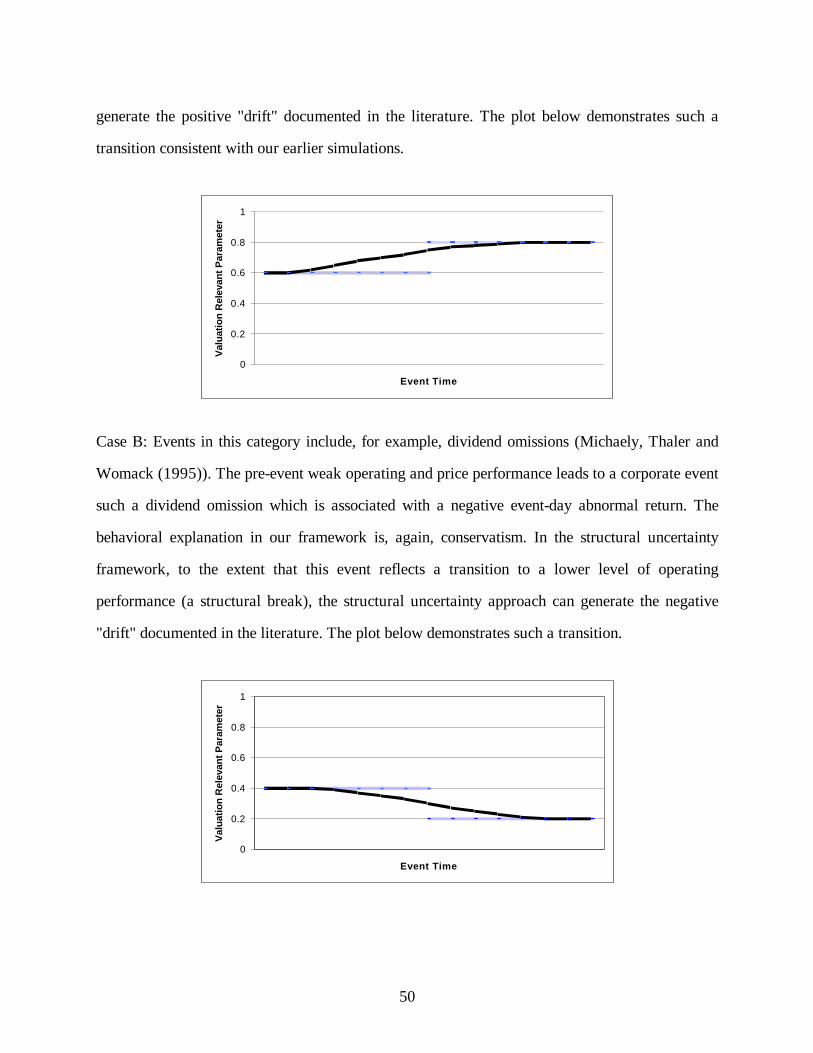
50

generate the positive "drift" documented in the literature. The plot below demonstrates such a

transition consistent with our earlier simulations.

0

0.2

0.4

0.6

0.8

1

Event Time

Val

uatio

n R

elev

ant P

aram

eter

Case B: Events in this category include, for example, dividend omissions (Michaely, Thaler and

Womack (1995)). The pre-event weak operating and price performance leads to a corporate event

such a dividend omission which is associated with a negative event-day abnormal return. The

behavioral explanation in our framework is, again, conservatism. In the structural uncertainty

framework, to the extent that this event reflects a transition to a lower level of operating

performance (a structural break), the structural uncertainty approach can generate the negative

"drift" documented in the literature. The plot below demonstrates such a transition.

0

0.2

0.4

0.6

0.8

1

Event Time

Val

uatio

n R

elev

ant P

aram

eter

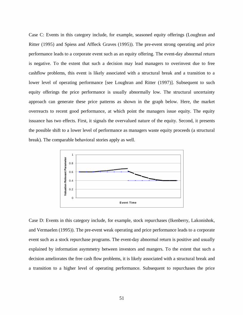
51

Case C: Events in this category include, for example, seasoned equity offerings (Loughran and

Ritter (1995) and Spiess and Affleck Graves (1995)). The pre-event strong operating and price

performance leads to a corporate event such as an equity offering. The event-day abnormal return

is negative. To the extent that such a decision may lead managers to overinvest due to free

cashflow problems, this event is likely associated with a structural break and a transition to a

lower level of operating performance [see Loughran and Ritter (1997)]. Subsequent to such

equity offerings the price performance is usually abnormally low. The structural uncertainty

approach can generate these price patterns as shown in the graph below. Here, the market

overreacts to recent good performance, at which point the managers issue equity. The equity

issuance has two effects. First, it signals the overvalued nature of the equity. Second, it presents

the possible shift to a lower level of performance as managers waste equity proceeds (a structural

break). The comparable behavioral stories apply as well.

0

0.2

0.4

0.6

0.8

1

Event Time

Val

uatio

n R

elev

ant P

aram

eter

Case D: Events in this category include, for example, stock repurchases (Ikenberry, Lakonishok,

and Vermaelen (1995)). The pre-event weak operating and price performance leads to a corporate

event such as a stock repurchase programs. The event-day abnormal return is positive and usually

explained by information asymmetry between investors and mangers. To the extent that such a

decision ameliorates the free cash flow problems, it is likely associated with a structural break and

a transition to a higher level of operating performance. Subsequent to repurchases the price

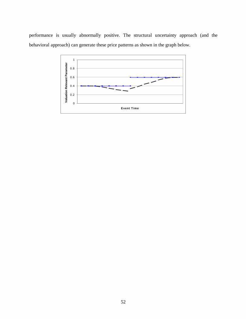
52

performance is usually abnormally positive. The structural uncertainty approach (and the

behavioral approach) can generate these price patterns as shown in the graph below.

0

0.2

0.4

0.6

0.8

1

Event Time

Val

uatio

n R

elev

ant P

aram

eter

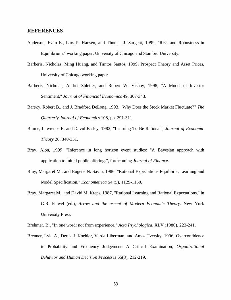
53

REFERENCES

Anderson, Evan E., Lars P. Hansen, and Thomas J. Sargent, 1999, "Risk and Robustness in

Equilibrium," working paper, University of Chicago and Stanford University.

Barberis, Nicholas, Ming Huang, and Tantos Santos, 1999, Prospect Theory and Asset Prices,

University of Chicago working paper.

Barberis, Nicholas, Andrei Shleifer, and Robert W. Vishny, 1998, "A Model of Investor

Sentiment," Journal of Financial Economics 49, 307-343.

Barsky, Robert B., and J. Bradford DeLong, 1993, "Why Does the Stock Market Fluctuate?" The

Quarterly Journal of Economics 108, pp. 291-311.

Blume, Lawrence E. and David Easley, 1982, "Learning To Be Rational", Journal of Economic

Theory 26, 340-351.

Brav, Alon, 1999, "Inference in long horizon event studies: "A Bayesian approach with

application to initial public offerings", forthcoming Journal of Finance.

Bray, Margaret M., and Eugene N. Savin, 1986, "Rational Expectations Equilibria, Learning and

Model Specification," Econometrica 54 (5), 1129-1160.

Bray, Margaret M., and David M. Kreps, 1987, "Rational Learning and Rational Expectations," in

G.R. Feiwel (ed.), Arrow and the ascent of Modern Economic Theory. New York

University Press.

Brehmer, B., "In one word: not from experience," Acta Psychologica, XLV (1980), 223-241.

Brenner, Lyle A., Derek J. Koehler, Varda Liberman, and Amos Tversky, 1996, Overconfidence

in Probability and Frequency Judgement: A Critical Examination, Organizational

Behavior and Human Decision Processes 65(3), 212-219.

54

Campbell, John, and John H. Cochrane, 1999, “By Force of Habit: A Consumption-Based

Explanation of Aggregate Stock Market Behavior,” Journal of Political Economy 107(2),

205-251.

Caskey, John, 1985, "Modeling the formation of price expectations: A Bayesian approach", The

American Economic Review 75 (4), 768-776.

Casella, George, and Roger L. Berger, 1990, Statistical Inference (Wadsworth and Brooks/Cole).

Chan, Louis K.C. Chan, Narasimhan Jegadeesh, and Josef Lakonishok, 1996, "Momentum

Strategies," Journal of Finance 51, 1681-1713.

Constantinides, George, 1990, “Habit Formation: A Resolution of the Equity Premium Puzzle,”

Journal of Political Economy 98(3), 519-543.

Cosmides, Leda, and John Tooby, 1994, “Better Than Rational: Evolutionary Psychology and the

Invisible Hand,” American Economic Review 84, 327-332.

Cosmides, Leda, and John Tooby, 1996, "Are Humans Good Intuitive Statisticians After All?

Rethinking Some Conclusions From the Literature on Judgement Under Uncertainty,"

Cognition 58, 1-73.

Daniel, Kent, David Hirshleifer, and A. Subrahmanyam, 1998, "A Theory of Overconfidence,

Self-Attribution, and Security Market Under- and Over-Reactions, Journal of Finance.

DeBondt, Werner F.M., and Richard H. Thaler, 1985, "Does the Stock Market Overreact,"

Journal of Finance 40, pp. 793-807, in Richard H. Thaler, ed., Advances in Behavioral

Finance, Russell Sage (1993).

Easterbrook, F. H. and Fischel, D. R., 1991, The economic structure of corporate law, Harvard

University Press, Cambridge, Massachusetts and London, England.

55

Edwards, Ward, 1968, "Conservatism in human information processing. In: Kleinmutz, B.(Ed.),

Formal Representation of Human Judgement. John Wiley and Sons, New York, pp. 17-52.

Fama, Eugene F., 1998, "Market Efficiency, Long-Term Returns, and Behavioral Finance,"

Journal of Financial Economics 49, 283-306.

Friedman, Benjamin M., 1979, "Optimal Expectations and the Extreme Information Assumptions

of 'Rational Expectations' Macromodels," Journal of Monetary Economics 5, pp. 23-41.

Gigerenzer, Gerd, 1991, How to make cognitive illusions disappear: Beyond heuristics and biases,

European Review of Social Psychology 2, 83-115

Grether, David M., 1980, “Bayes Rule As A Descriptive Model: The Representativeness

Heuristic,” The Quarterly Journal of Economics.

Griffin, Dale, W., and Amos Tversky, 1992, The Weighting of Evidence and the Determinants of

Confidence, Cognitive Psychology 24, 411-435.

Griffin, Dale, W., and Carol A. Varey, 1996, Towards a Consensus on Overconfidence,

Organizational Behavior and Human Decision Processes 65(3), 227-231.

Griffin, Dale, W., and Roger Buehler, 1999, Frequency, Probability, and Prediction: Easy

Solutions to Cognitive Illusions?, Cognitive Psychology 38, 48-78.

Grullon, Gustavo, Roni Michaely, and Bhaskaran Swaminathan, 1999, Are Dividends a Sign of

Firm Maturity?, working paper Cornell University.

Hansen, Lars P., Thomas J. Sargent, and Thomas D. Tallarini, 2000, "Robust Permanent Income

and Pricing," Review of Economic Studies, forthcoming.

Hansen, Lars P., Thomas J. Sargent, and Neng E. Wang, 2000, "Robust Permanent Income and

Pricing with Filtering," working paper, University of Chicago and Stanford University.

56

Haugen, Robert A., 1999, The New Finance: The Case Against Efficient Markets, 2nd ed.

Prentice Hall.

Hong, Harrison, and Jeremy Stein, 1999, "A unified theory of underreaction, momentum trading,

and overreaction in asset markets," Journal of Finance 54(6), 2143-2184.

Ikenberry, David, Josef Lakonishok, and Theo Vermaelen, 1995, "Market underreaction to open

market share repurchases," Journal of Financial Economics 39, 181-208.

Jegadeesh, Narasimhan, and Sheridan Titman, 1993, "Returns to Buying Winners and Selling

Losers: Implications for Stock Market Efficiency," Journal of Finance 48, 65-91.

Jolls, Christine, Cass R. Sunstein, and Richard Thaler, 1998, “A Behavioral Approach to Law and

Economics,” Stanford Law Review, 50(5), 1471-1550.

Kurz, Mordecai, 1994, “On the structure and diversity of rational beliefs,” Econ. Theory 4, 877-

900.

Lakonishok, Josef, Andrei Shliefer, and Robert W. Vishny, 1994, "Contrarian Investment,

Extrapolation, and Risk," Journal of Finance 49, 1541-1578.

Lewellen, Jonathan, and Jay Shanken, 1999, "Estimation risk, market efficiency, and the

predictability of returns", working paper, University of Rochester.

Lewis, Karen K., 1989, "Changing beliefs and systematic rational forecast errors with evidence

from foreign exchange", The American Economic Review 79, 621-636.

Loughran, Tim, and Jay R. Ritter, 1995, "The new issues puzzle", Journal of Finance 50, 23-51.

Loughran, Tim, and Jay R. Ritter, 1997, "The Operating Performance of Firms Conducting

Seasoned Equity Offerings," Journal of Finance, Vol. 52(5), 1823-1850.

Mayfield, Scott, 1999, “Estimating the Market Risk Premium,” working paper, Harvard Business

School.

57

McCloskey, Donald N., 1983, “The Rhetoric of Economics,” Journal of Economic Literature,

21(2), 481-517.

Merton, Robert C., 1980, "On Estimating the Expected Return On the Market: An Exploratory

Investigation," Journal of Financial Economics 8, 323-361.

Merton, Robert C., 1987, "A Simple Model of Capital Market Equilibrium with Incomplete

Information," Journal of Finance, 42(3), 483-510.

Michaely, Roni, Richard H. Thaler, and Kent L. Womack, 1995, "Price Reactions to Dividend

Omissions: Overreaction or Drift?," Journal of Finance, 50(2), 573-608.

Miller, Edward M., 1977, "Risk, Uncertainty, and Divergence of Opinion," Journal of Finance,

32(4), 1151-1168.

Morris, Stephen, 1996, "Speculative Investor Behavior and Learning," Quarterly Journal of

Economics, 111(4), 1111-1134.

Nyarko, Yaw, 1991, "Learning in Misspecified Models and the possibility of Cycles," Journal of

Economic Theory 55, 416-427.

O'dean, Terrance, 1998, "Volume, Volatility, Price, and Profit When All Traders Are Above

Average," Journal of Finance, 53, 1887-1934.

Pastor, Lubos and Robert F. Stambaugh, 1998, "The equity premium and structural breaks",

working paper, University of Pennsylvania.

Pontiff, Jeffrey, 1996, " Costly Arbitrage: Evidence from Closed-End Funds," Quarterly Journal

of Economics 111(4), 1135-1151.

Sargent, Thomas J., 1993, Bounded Rationality in Macroeconomics. Oxford University Press.

58

Shiller, Robert J., 1981, “Do Stock Prices Move Too Much To Be Justified By Subsequent

Changes in Dividends?” American Economic Review 71(3), 421-436, in Richard H.

Thaler, ed., Advances in Behavioral Finance, Russell Sage (1993).

Shleifer, Andrei and Robert W. Vishny, 1997, "The Limits of Arbitrage", Journal of Finance

Smith, A.F.M., 1975, “A Bayesian Approach To Inference About a Change-Point in a Sequence

of Random Variables,” Biometrika, 62(2), pp. 407-416.

Spiess, Katherine D., and John Affleck-Graves, 1995, "Underperformance in Long-Run Stock

Returns Following Seasoned Equity Offerings," Journal of Financial Economics 38(3),

243-67.

Stein, Jeremy, 1996, "Rational Capital Budgeting in an Irrational World", Journal of Business,

69, pp. 429-455.

Thaler, Richard H., ed., 1993, Advances in Behavioral Finance, Russell Sage.

Timmerman, Allan, 1993, "How Learning in Financial Markets Generates Excess Volatility and

Predictability in Stock Prices," Quarterly Journal of Economics 108, 1135-1145.

Tooby, John, and Leda Cosmides, 1992, “The Psychological Foundations of Culture,” in Jerome

H. Barkow, Leda Cosmides, John Tooby, 1992, The Adapted Mind, Oxford University

Press.

Veronesi, Pietro, 1999, “Stock Market Overreaction to Bad News in Good Times: A Rational

Expectations Equilibrium Model,” Review of Financial Studies 12(5), 975-1007.

Williams, Joseph T., 1977, "Capital Asset Prices with Heterogeneous Beliefs," Journal of

Financial Economics 5, 219-239.

Winkler, Robert L. and Allan H. Murphy, 1973, “Experiments in the Laboratory and the Real

World,” Organizational Behavior and Human Performance 10, 252-270.