Comparison of Three Interpolation

Schemes to Generate Daily and

Monthly Gridded Precipitation

Analyses by the Global

Precipitation Climatology Centre

(GPCC) and its Application to

Produce Global Analyses

Deutscher Wetterdienst, Global Precipitation Climatology Centre, Offenbach, Germany

Ziese, M.; Schneider, U.; Meyer-Christoffer, A.; Rustemeier, E.; Finger, P.; Schamm, K.;

Becker, A.

Background of GPCC

Collection, quality control and storage of observations, generation of gridded

analyses

Established at the beginning of 1989 at Deutscher Wetterdienst (DWD) on

invitation by WMO → more than 25 years of experience with precipitation

Analysis of precipitation on the basis of in-situ data for the land-surface

Contributing to GEWEX (Global Energy and Water Exchanges Project), GCOS

(Global Climate Observing System) and land-analysis for GPCP

Many users world wide, analyses used in IPCC-AR5

Data sources:

SYNOP, CLIMAT, SYNOP from CPC

national meteorological services

CRU, FAO, GHCN

ECA&D, regional data collections 2

GPCC data basis

3

Monthly totals, collection since 1989

Daily totals, collection since 2012

Problems detected

Stations are sometimes located in the ocean or outside of the boundaries of

the country

Unusual annual cycle or extreme outliers of monthly precipitation

Temporal shifts in the data

Factor*10 errors

Typing or coding errors

Errors in the conversion of inch, mm etc. (mostly with historical data)

Incorrect flagging of missing precipitation observations (might be

misinterpreted as „0“)

4

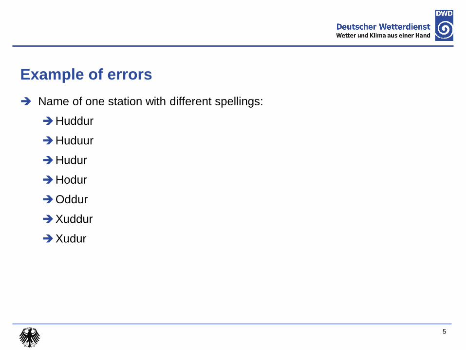
Example of errors

Name of one station with different spellings:

Huddur

Huduur

Hudur

Hodur

Oddur

Xuddur

Xudur

5

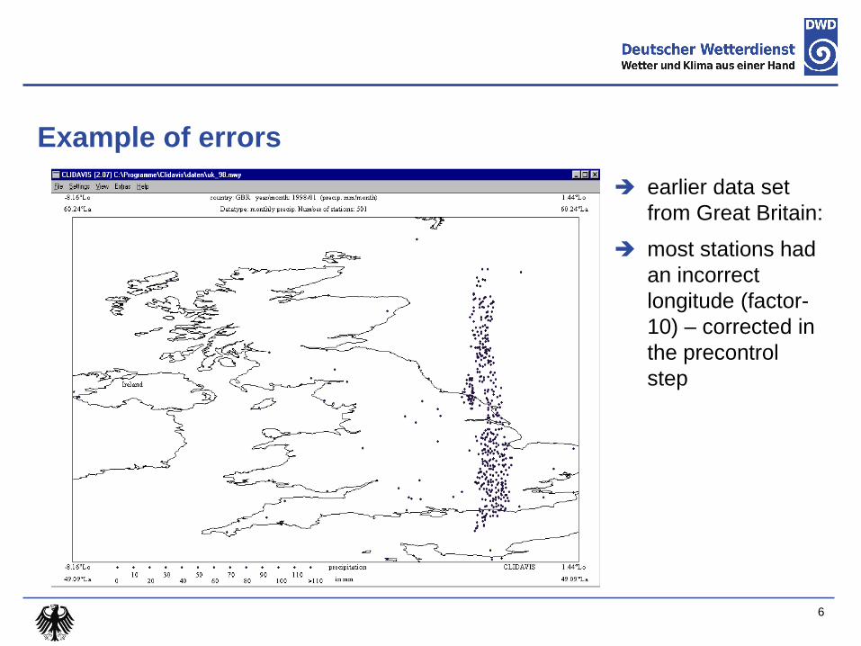
Example of errors

earlier data set

from Great Britain:

most stations had

an incorrect

longitude (factor-

10) – corrected in

the precontrol

step

6

Example of errors

Data shifted by one day

7

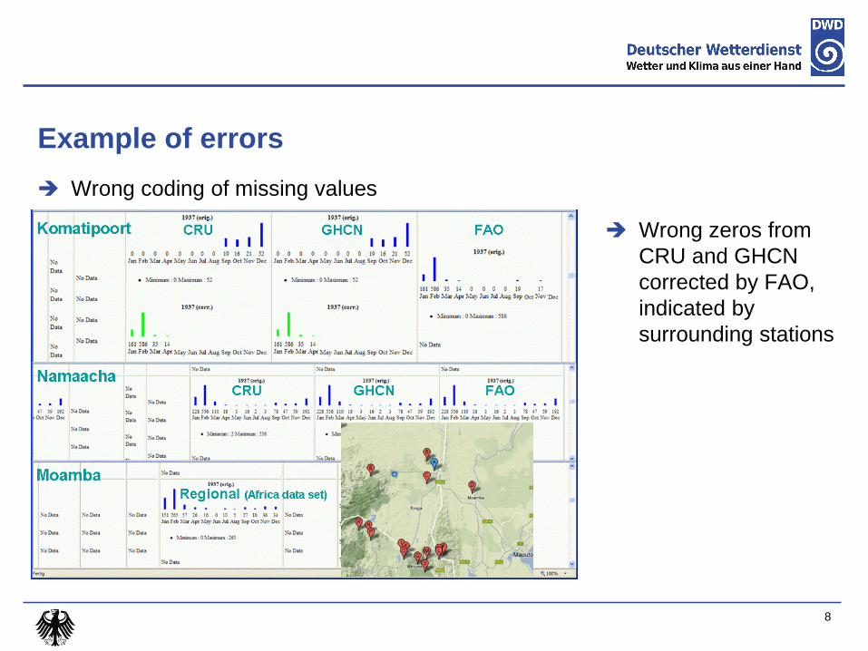
Example of errors

Wrong coding of missing values

8

Wrong zeros from

CRU and GHCN

corrected by FAO,

indicated by

surrounding stations

Example of errors

Shift in time

9

1982 1980

1953 1952 1951

1979

Comparison of Interpolation Schemes

used interpolation schemes:

modified SPHEREMAP

ordinary Kriging

arithmetic mean

two test months: July 1986 and January 1987

population divided into collectives with 300 stations

using 4800 stations as reference

50 runs with arbitrary selected reference stations to calculate skill scores

stepwise reduction of station density (input stations, not reference stations)

4 to 10 input stations

runs with interpolation of anomalies and absolute values

reduced station density in Germany (219 instead of more than 4000)

10

Kriging (Krige 1966)

statistical interpolation scheme

calculates correlations on basis of variograms

used for daily data sets at GPCC

uses at least 4, at most 10 stations

search radius depends on station density

applies only one variogram for global interpolations

11

SPHEREMAP (Willmott et al. 1985)

Application for monthly data sets at GPCC

Combination of distance and angular weighting

Distance weighting similar to IDW with given empirical weighting functions

Angular weighting to reduce influence of clustered stations

Compute gradients to preserve non-observed extremes

12

𝑆1 𝑆2 𝑆3 𝑆4 𝑤1 > 𝑤2 > 𝑤3 > 𝑤4

𝑆1

𝑆2

𝑆3 𝑆5 𝑤1, 𝑤2 > 𝑤3, 𝑤4, 𝑤5

Grid

point

Grid

point

𝑆4

𝑆1 𝑆2 𝑆3 𝑆4 Grid

point

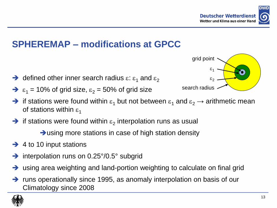
SPHEREMAP – modifications at GPCC

13

defined other inner search radius : 1 and 2

1 = 10% of grid size, 2 = 50% of grid size

if stations were found within 1 but not between 1 and 2 → arithmetic mean

of stations within 1

if stations were found within 2 interpolation runs as usual

using more stations in case of high station density

4 to 10 input stations

interpolation runs on 0.25°/0.5° subgrid

using area weighting and land-portion weighting to calculate on final grid

runs operationally since 1995, as anomaly interpolation on basis of our

Climatology since 2008

grid point

1

2

search radius

Interpolation of anomalies or totals

Interpolation of anomalies:

Deviation from long term means interpolated, finally added to gridded long

term means

Also known as ‚Climatological Aided Interpolation‘ (CAI)

Need for many and long data series to compute long term means

Advantage: better results, also in data sparse regions

Interpolation of totals:

Observations are interpolated

Worse in data sparse regions

14

Possible anomalies

‚absolute‘ anomalies:

Observation minus long term mean

Suitable for monthly data

‚relative‘ anomalies:

Observation divided by monthly total or long term mean

Qualified for daily data

15

Used skill scores

mean squared error (MSE)

[MSE] = mm²/month²

sensitive to outliers

n

K

kk oyn

MSE1

2)(*1

mean absolute error (MAE)

[MAE] = mm/month

measure of average error

n

k

kk oyn

MAE1

*1

o – observed value at station

y – interpolated value at station

n - number of stations

16

Comparison July 1986

17

anomaly interpolation better than absolute interpolation

modified SPHEREMAP best for absolute interpolation (Climatology)

Comparison January 1987

18

anomaly interpolation better than absolute interpolation

modified SPHEREMAP best for absolute interpolation (Climatology)

Comparison SPHEREMAP and Kriging July 1986

Kriging modified SPHEREMAP

Kriging - SPHEREMAP

overall patterns look

similar

Kriging produces

smoother patterns

most differences due

to different gradients

of precipitation and in

data sparse areas

19

Comparison of interpolation schemes, daily precipitation

Comparison of

different

interpolation

schemes with

cross-validation

Separation

according to

Köppen-Geiger

climate zones

Best results for

ordinary kriging

with anomalies

Gridded GPCC products

Different products to tailor diverse user needs

Provide gridded analyses, no station data (except ITD)

21

Precipitation Standard deviation

Stations per grid Kriging error

Full Data Daily, 1997/07/06

22

Undercatch correction factor

Fraction solid precipitation

Stations per grid

Precipitation

Monitoring Product, 2015/05

23

Climatology, July

0.25°

1.0°

0.5°

2.5°

24

Suggestions for the interpolation of:

Daily minimum temperature (0.6 K/100 m)

Daily maximum temperature (0.6 K/100 m)

Wind speed

Vapor pressure (0.025 hPa/100 m)

Solar radiation

Lapse rate

Elevation correction

25

26

Zusätzliche Folien

27

First Guess Daily, First Guess Monthly

First Guess Daily, 2015/07/02 First Guess Monthly, 2015/07

28

GPCC quality control

29

SYNOP

SYNOP + CLIMAT

Historical data

Automatic quality control using region depended

fixed thresholds, consistence checks of overlapping

intervals and weather observations; delete

questionable observations; fill gaps

Automatic quality control using region depended

fixed thresholds; mark questionable observations

for manuel checks, result: confirm, correct or

delete values

Test against station and grid based statistical

thresholds; mark questionalbe observations for

manuel checks, result: confirm, correct or delete

values; spatial consistence of extreme values

non-used Stations in modified SPHEREMAP

grid point

1

2

used station

non-used station

0.25°/0.5°

30

Data base GPCC – spatial coverage

31

All stations in data bank

More than 100,000 stations

AOPC

OOPC

TOPC

Data base GPCC – spatial coverage

Locations of 75 631 stations and lengths of their precipitation records

Only stations with records longer than 10 years, beginning no earlier than 1814

32

Figure 18 from GCOS report 195: Status of the Global Observing System for Climate, Full Report October 2015

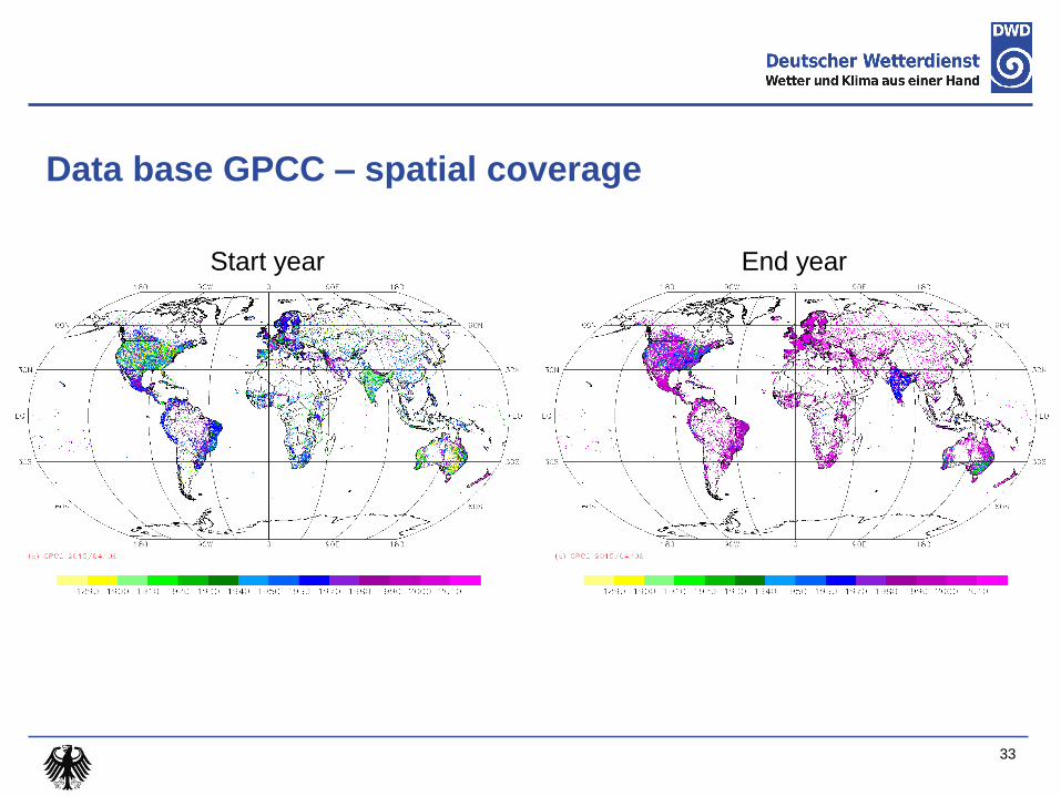
Data base GPCC – spatial coverage

33

Start year End year

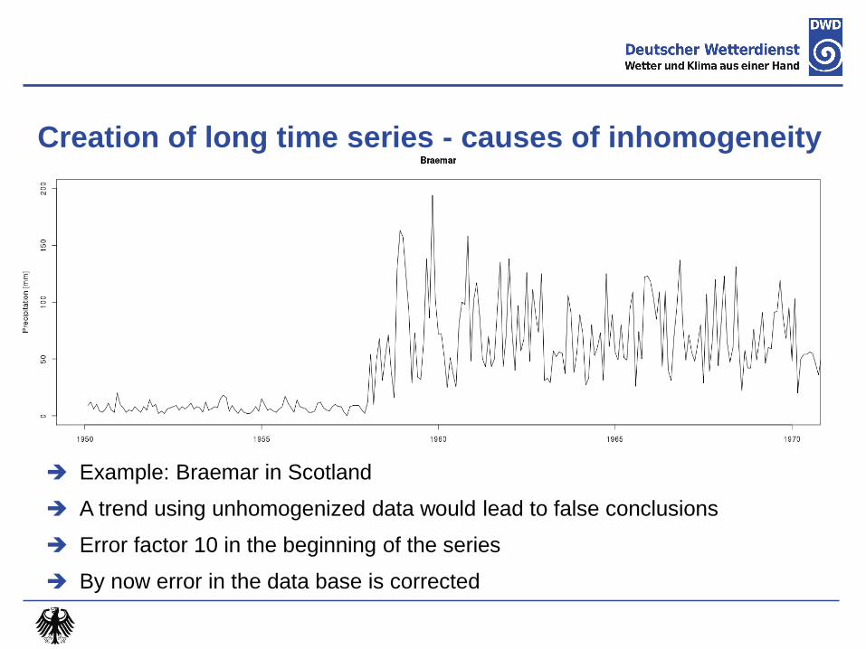
Creation of long time series - causes of inhomogeneity

Example: Braemar in Scotland

A trend using unhomogenized data would lead to false conclusions

Error factor 10 in the beginning of the series

By now error in the data base is corrected

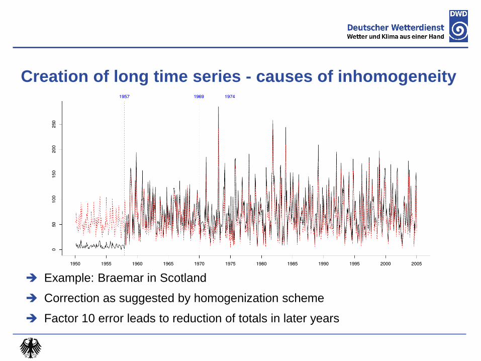
Creation of long time series - causes of inhomogeneity

Example: Braemar in Scotland

Correction as suggested by homogenization scheme

Factor 10 error leads to reduction of totals in later years

Anwendungsbeispiel: Vergleich von Bezugszeiträumen

Für jeden Bezugszeitraum

selben Stationen verwendet

10 Datenjahre dürfen pro

Bezugszeitraum fehlen

Daten nicht homogenisiert

Großräumige Muster gleich

36

1951-1980 1961-1990

1971-2000 1981-2010 Stationsbasis

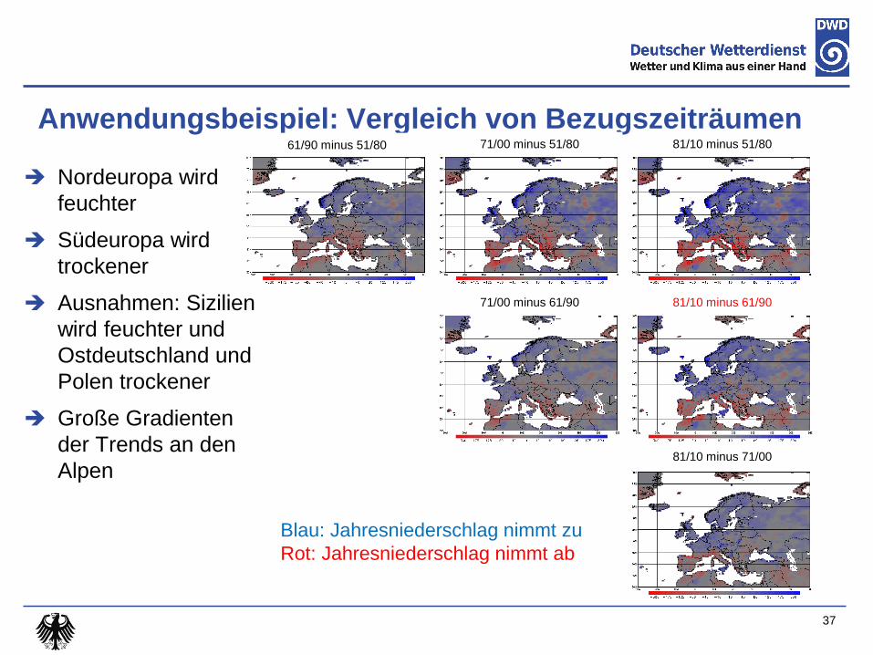
Anwendungsbeispiel: Vergleich von Bezugszeiträumen

Nordeuropa wird

feuchter

Südeuropa wird

trockener

Ausnahmen: Sizilien

wird feuchter und

Ostdeutschland und

Polen trockener

Große Gradienten

der Trends an den

Alpen

37

61/90 minus 51/80 71/00 minus 51/80 81/10 minus 51/80

71/00 minus 61/90 81/10 minus 61/90

81/10 minus 71/00

Blau: Jahresniederschlag nimmt zu

Rot: Jahresniederschlag nimmt ab

Beispiel: Full Data Monthly, 1997/07

Niederschlag

Stationsanzahl pro Raster

38

Beispiel: Interpolation Test Dataset (ITD), Juli

Niederschlag

Stationsanzahl pro Raster

39

WZN-Dürreindex

GPCC-DI: gerasterter Dürreindex mit beinahe globaler Abdeckung

Kombination von SPI-DWD und SPEI

Niederschlagsdaten vom WZN; First Guess Monthly

Monatsmitteltemperatur vom CPC

Verwendet Mittelwert von SPI-DWD und SPEI, falls beide berechnet werden

können, sonst nur den berechenbaren Index

Parameter basieren auf Full Data Monthly V.6, Referenzperiode 1961-1990

Mehrere Aggregationszeiträume: 1, 3, 6, 9, 12, 24 und 48 Monate

Verwendet nur gerasterte Felder, keine Interpolationen

Zurück bis Januar 2013 verfügbar

Abgabe im netCDF-Format

Wird am 10. bis 13. Tag des Folgemonats aktualisiert

40

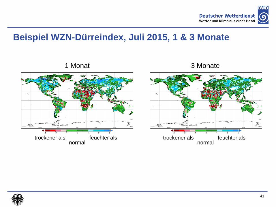
Beispiel WZN-Dürreindex, Juli 2015, 1 & 3 Monate

normal feuchter als trockener als

1 Monat 3 Monate

normal feuchter als trockener als

41

Example of errors

Wrong metadata (longitude)

42

Example of errors

Repeating data

43

Example of errors

Interchange

between

stations

44

Example of errors

Filled gaps with data from climatology

45

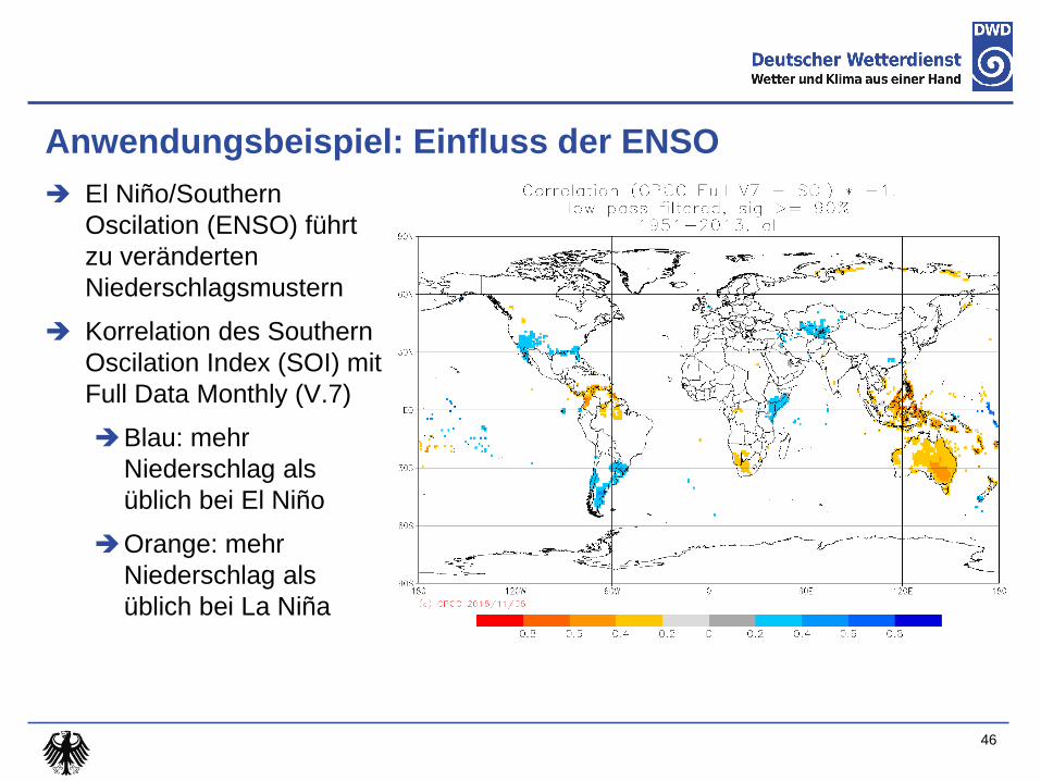
Anwendungsbeispiel: Einfluss der ENSO

El Niño/Southern

Oscilation (ENSO) führt

zu veränderten

Niederschlagsmustern

Korrelation des Southern

Oscilation Index (SOI) mit

Full Data Monthly (V.7)

Blau: mehr

Niederschlag als

üblich bei El Niño

Orange: mehr

Niederschlag als

üblich bei La Niña

46

Anwendungsbeispiel: Einfluss der ENSO (Frühjahr)

47

Anwendungsbeispiel: Einfluss der ENSO (Sommer)

48

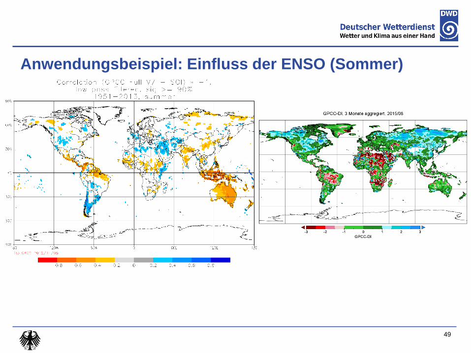
Anwendungsbeispiel: Einfluss der ENSO (Sommer)

49

Anwendungsbeispiel: Einfluss der ENSO (Herbst)

50

Anwendungsbeispiel: Einfluss der ENSO (Herbst)

51

Anwendungsbeispiel: Einfluss der ENSO (Winter)

52

Anwendungsbeispiel: Einfluss der ENSO (Winter)

53

Anwendungsbeispiel: Dürre in Kalifornien

54

GPCC-DI, Niederschlag über 12 Monate aggregiert

2011 2012 2013

2014 2015

Anwendungsbeispiel: Dürre in Sao Paulo Vorzeitiges Ende der Regenzeit 2013/2014

Später Anfang und trockenere Regenzeit

2014/2015

Wassermangel für Bevölkerung und Industrie

Einfluss von Klimawandel und ENSO werden

noch diskutiert

55

Anwendungsbeispiel: Trends in der Dürrehäufigkeit

Änderung der

Anzahl der Dürren in

62 Jahren, nicht der

Intensität

3 Monate

aggregiert, Dürre

über 5 Monate

wurde dreimal

gezählt

Blau: Dürren werden

seltener

Braun: Dürren

werden häufiger

Trends in Europa

passen zu Trends

im Niederschlag

56

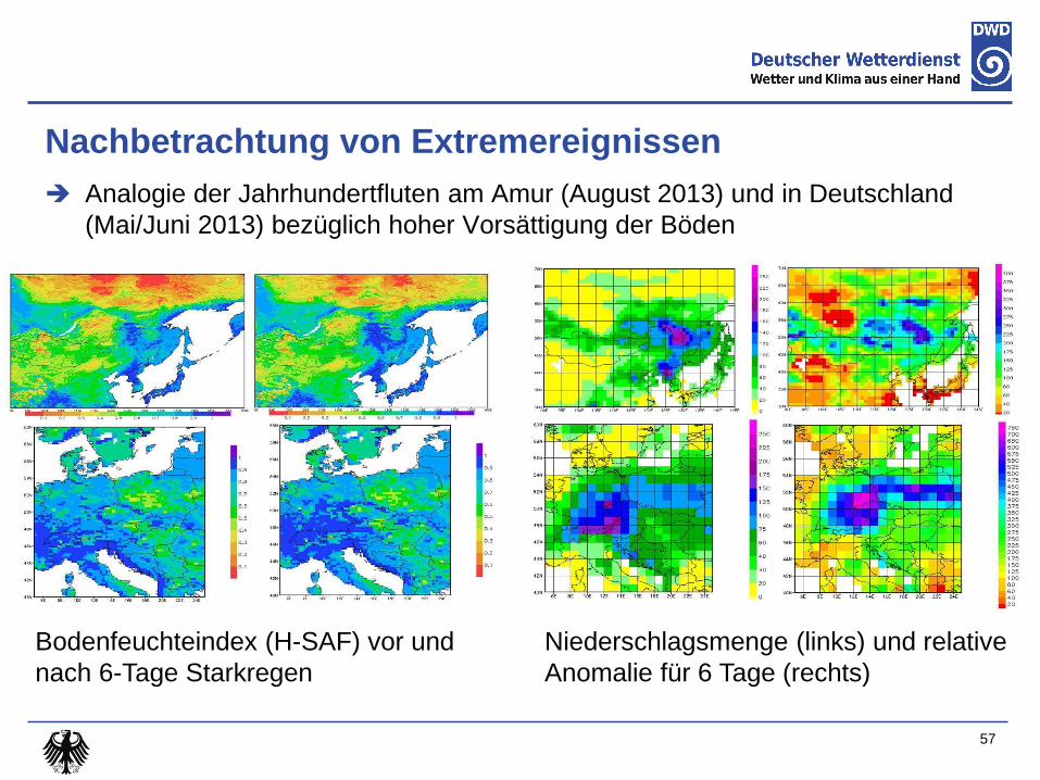
Nachbetrachtung von Extremereignissen

Analogie der Jahrhundertfluten am Amur (August 2013) und in Deutschland

(Mai/Juni 2013) bezüglich hoher Vorsättigung der Böden

57

Bodenfeuchteindex (H-SAF) vor und

nach 6-Tage Starkregen

Niederschlagsmenge (links) und relative

Anomalie für 6 Tage (rechts)