Comparison of the reliability index between American codes ...

Comparison of the reliability index between American codes and Chinese codes

by

Haofan Zhao

A thesis submitted to the Graduate Faculty of

Auburn University

in partial fulfillment of the

requirements for the Degree of

Master of Science

Auburn, Alabama

December 15, 2018

Keywords: reliability analysis, Chinese code, American code,

limit state design, reinforced concrete structures

Copyright 2018 by Haofan Zhao

Approved by

Andrzej Nowak, Chair, Professor of Civil Engineering

J. Michael Stallings, Professor of Civil Engineering

Robert Barnes, Associate Professor of Civil Engineering

ii

Abstract

The primary purpose of this research is to apply the reliability analysis techniques to the

evaluation of two different series’ structural design codes using in America and China. This

research is focused on two kinds of structures: beams and columns. For the objective, eight

calculation examples were generated. They would be separately designed by Chinese codes

(the GB50010-2010 & GB50009-2012) and American codes (ASCE 7-10 and ACI318-14). In

the eight calculation examples, two of them were beam structures and the others were column

structures.

The GB 50010-2010 is the national code for design of concrete structures in China. The

GB50009-2012 is the load code for design of building structures. They are widely used in

structural design in China. The examples designed by Chinese codes would progress the load

combination and determine the required resistance by GB50009-2012 (load code for design of

building structures). Afterward, according to the GB50010-2010, reinforcement ratios were

estimated. For the examples designed by American codes, the load combination and required

resistance would be determined by ASCE 7-10, reinforcement ratio would be calculated based

on ACI 318-14.

In this research, the Monte Carlo method was used to evaluate the reliability index for

examples. Then the reliability index for each example was applied to the sensitivity analysis,

the results of which would give a good view for comparison of the two series’ codes.

iii

Acknowledgments

First, I would give appreciation to Dr. Andrzej S. Nowak, my advising professor. Without

his advice and guidance, I could not finish my thesis so successfully. I thoroughly enjoyed

spending time with him, and I am fortunate to have him as my advisor.

I would also like to thank Dr. Michael Stallings and Dr. Robert Barnes for serving on my

thesis committee. I really appreciate that I could have opportunities to have their classes during

my graduate campus life and the knowledge I learned from them benefited my thesis a lot.

Next, I would like to thank everyone who helped me. Some of them helped me to prepare

the defense, some of them helped me to arrange my schedule, etc. They didn’t directly help me

with my study, but their help was significant to my thesis. I might not have been able to finish

my thesis in time without anyone who helped me. I am also thankful to my parents, who

supported me to study in Auburn. Without their support and help, I could never have gotten the

achievement today.

iv

Table of Contents

Abstract ......................................................................................................................... ii

Acknowledgments ....................................................................................................... iii

List of Tables ............................................................................................................... vi

List of Abbreviations ................................................................................................ viii

1. Introduction .......................................................................................................... 1

1.1. Overview .................................................................................................................... 1

1.2. Objective..................................................................................................................... 1

1.3. Introduction of Chinese codes and American codes ................................................... 2

1.4. Scope and research approach ...................................................................................... 3

1.5. Organization of the research ....................................................................................... 3

2. Loads ...................................................................................................................... 5

2.1. Load design methods and requirements in Chinese code (GB 5009-2012) ............... 5

2.1.1. Requirements and calculation functions of loads in GB 50009-2012 ............................. 6

2.1.2. Load combination in GB 50009-2012........................................................................... 11

2.1.3. Statistical parameters of loads in GB5009-2012 ........................................................... 13

2.2. Load design methods and requirements in American code (ASCE 7-10) ................ 14

2.2.1. Requirements and calculation functions of loads in ASCE 7-10 .................................. 14

2.2.2. Load Combination in ASCE 7-10 ................................................................................. 16

2.2.3. Statistical parameters of loads in ASCE 7-10 ............................................................... 17

3. Resistance of reinforced concrete beam ........................................................... 18

3.1. Beam resistance design method in GB 50010-2010 ................................................. 18

3.2. Beam resistance design method in ACI 318-14 ....................................................... 19

3.3. Statistical parameters of moment resistance ............................................................. 20

4. Resistance of reinforced concrete column ........................................................ 23

4.1. Column resistance design method in ACI 318 ......................................................... 23

4.2. Column resistance design method in GB 50010-2010 ............................................. 29

4.3. Statistical parameters of column resistance .............................................................. 38

5. Reliability analysis .............................................................................................. 40

6. Comparison of Chines codes and American codes .......................................... 43

6.1. Examples of reliability comparison .......................................................................... 43

6.2. Reliability indexes of Chinese codes ........................................................................ 47

v

6.2.1. Reliability index of beam designed by Chinese codes .................................................. 47

6.2.2. Reliability indexes of columns designed by Chinese codes .......................................... 48

6.3. Reliability indexes of American codes ..................................................................... 50

6.3.1. Reliability index of beam designed by American codes ............................................... 50

6.3.2. Reliability indexes of columns designed by American codes ....................................... 51

6.4. Comparison of sensitive analysis ............................................................................. 53

6.4.1. Sensitive analysis of beams ........................................................................................... 53

6.4.2. Sensitive analysis of columns ....................................................................................... 56

7. Conclusions ......................................................................................................... 59

References ................................................................................................................... 61

vi

List of Tables

Table 1- Regular materials self-weight ........................................................................ 6

Table 2- Norminal value of live load , combination value, frequent value and quasi-

permanent value ........................................................................................................... 6

Table 3- Basic snow pressure in Beijing...................................................................... 7

Table 4- Basic wind pressure in Beijing ...................................................................... 8

Table 5- Factor k and α1 ........................................................................................ 10

Table 6- the variety factor of the different height for wind pressure ......................... 11

Table 7- Statistical parameter of loads in GB5009-2012 ........................................... 14

Table 8- Statistical parameter of loads in ASCE 7-10 ............................................... 17

Table 9- Statistical parameters of moment resistance in GB 50010-2010 ................. 21

Table 10- Statistical parameters of moment resistancce in ACI 318-14 ................... 22

Table 11- Statistical parameter for column resistance in GB 50010-2010 ................ 38

Table 12- Statistical parameter for column resistance in ACI 318-14 ....................... 39

Table 13- The axial force and bending moment for Example 3 and Example 4 ....... 45



Table 16- Reliability index for different reinforcement ratios ................................... 54

Table 17- Reliability index for ratio of live load versus dead load plus live load ..... 55

Table 18- Reliability index due to different concrete strength of Example 3 and

Example 4 .................................................................................................................. 56

Table 19- Reliability index due to different reinforcement ratio of Example 3 and

Example 4 .................................................................................................................. 57

vii

List of Figures

Fig 1. Moment resistance details in GB 50010-2010 ................................................ 18

Fig 2. Moment resistance details in ACI 318-14 ....................................................... 20

Fig 3. Strain and stress distribution in cross-section of an eccentrically loaded column.

...................................................................................................................................... 31

Fig 4. Interaction diagram of column ........................................................................ 32

Fig 5. Beam example: simple support beam .............................................................. 43

Fig 6. The dimension of first floo for Example 3 and Example 4 ............................. 45

Fig 7. The dimension of first floor for Example 5 and Example 6 ............................ 46

Fig 8. The CDF of g of Example 1 ............................................................................ 48

Fig 9. CDF of g for Example 3 .................................................................................. 48

Fig 10. CDF of g for Example 3 neglected minimum reinforcement requirement ...... 49

Fig 11. CDF of g for Example 5 ................................................................................ 50


Fig 13. CDF of g of Example 2 .................................................................................. 51




Fig 17. Reliability index for different reinforcement ratios ....................................... 54

Fig 18. Reliability index for ratio of live load versus dead load plus live load ......... 55

Fig 19. Reliability index due to different concrete strength ...................................... 57

Fig 20. Reliability index due to different reinforcement ratios ................................. 58

viii

List of Abbreviations

AASHTO American Association of State Highway and Transportation Officials

ACI American Concrete Institute

ASCE American Society of civil engineers

GB National standards of People's Republic of China

1

1. Introduction

1.1. Overview

The reliability index is an essential parameter for the structure design. Reliability in the

structures is defined as “the probability of a device performing its purpose adequately for the

period of time intended under the operating conditions encountered” (Bazovsky, 1961).

Generally, the reliability index directly describes how stable the structures are. In addition, it

is also an important factor of economic control.

The reliability analysis is a kind of analytical technology based on statistics and

probability theory. With the statistical data, it can provide a value to represent how many

possibilities this structure will have a failure. Generally, 3.50 is the number of reliability when

the structures had enough resistance and excellent economic benefit. This research focused on

the reinforcement concrete beams and reinforced concrete columns. The actual concrete

structural element’s capacity is varying due to many factors, such as yield strength of steel

rebars, the compression strength of concrete, and dimensions of the structural elements. Actual

loads are also changed.

1.2. Objective

The main purpose of this research is to apply the reliability analysis techniques to the

evaluation of different series structural design codes (ACI 318-14, ASCE 7-10 and GB 50010-

2010, GB 50009-2012) and compare the reliability performances of the examples designed by

these two series’ codes. There would be two kinds of concrete component examples involved

in this research: reinforced concrete beam and reinforced concrete column. The beams’

2

examples would mainly show how the different loads’ design methods affect the reliability.

And the columns’ examples would mainly show how the different resistance design methods

affect the reliability.

1.3. Introduction of Chinese codes and American codes

The Chinese codes used to design and analyze were GB 5009-2012 “Load code for the

design of building structures” and GB 50010-2010 “Code for design of concrete structures.”

GB is the abbreviation for the Chinese National Standard. It is a series of design codes and

requirements for all kinds of engineer areas. GB 5009-2012 is the load's design code edited by

Ministry of Housing and Urban-Rural Development of the People's Republic of China. It is the

most official and widely used code for the load's design. GB 50010-2010 is the concrete

component structural design code, also edited by Ministry of Housing and Urban-Rural

Development of the People's Republic of China. It provides the minimum requirements of

structural concrete components. Any kinds of structural concrete components should meet the

requirements of GB 50010-2010 and required extra codes.

The American codes used to design and analyze were ASCE 7-10 “Minimum design

loads for buildings and other structures” and ACI 318-14 “Building code requirements for

structural concrete.” ASCE 7-10 is the load's design codes published by American Society of

Civil Engineering. It is only specific for building design. “It provided minimum loads

requirements for the design of buildings and other structures that are subject to building code

requirements” (American society of civil engineers, 2010). ACI 318-14 is the concrete

component design codes published by American Concrete Institute. It provides the minimum

requirements for materials, design and detailing of structural concrete building and, where

3

applicable, nonbuilding structures (American Concrete Institute, 2014). It is only specific for

building design like ASCE 7-10.

In this research, the examples for analysis were assumed as components of office buildings

and residential buildings. Each example applied different series codes for design and reliability

analysis. Due to different requirements in the codes, the performance of reliability had

significant differences.

1.4. Scope and research approach

For the purpose of this research, there were several different comparison examples. Due

to the limited research resources, the focus was on two types of structures: reinforced concrete

beams and reinforced concrete columns. There were two beams examples: one designed by GB

codes and another one designed by ACI and ASCE codes. The basic resistance design

principles are similar to each other with only a slight difference. There were six examples for

the columns. Half of them were designed by GB codes, while the others were designed by ACI

and ASCE codes. The reason for the number of column examples was that the resistance

requirements and design methods were entirely different from each other. Therefore, more

examples were required to cover all situations. Chapter four will discuss in more detail about

the resistance design method and chapter seven will provide detailed differences between the

two series’ codes. All of the examples will be applied the reliability analysis to calculate

reliability index. Then, the sensitivity analysis should be considered. Through the sensitivity

analysis results, it could be easier to get conclusions about the two series’ codes.

1.5. Organization of the research

This research is organized by seven chapters. Chapter one gives the brief introduction to

4

this report. It also includes the objective, introduction of design codes, scope and approach.

Chapter two illustrates the load design methods of GB 50010-2010 and ASCE 7-10. It also

provides load requirements, load combinations and statistical parameters in each code. Chapter

three reviews the beam resistance design methods of GB 5009-2012 and ACI 318-14, includes

resistance functions and statistical parameters for each factor. Chapter four introduces the

column design methods of GB 5009-2012 and ACI 318-14 while illustrating different

situations requirements in each code and provides the statistical parameters of factors. Chapter

five presents the procedure of reliability analysis and how it is to be applied to the examples.

Chapter six discusses the comparison between two series codes and compares the results after

reliability analyzing. Chapter seven will provide the conclusion from chapter two to chapter

six, briefly stating the advantages and disadvantages of the two series’ codes.

5

2. Loads

All the structural components are designed to have certain required resistance, which

should be larger than the design loads on the component. As a result, determining the design

loads is the first step in the procedure of finishing the component design. This chapter will

introduce the load requirements in GB 5009-2012 “Load code for the design of building

structures” and ASCE 7-10 “Minimum design loads for buildings and other structures” and

provide the statistical parameters for each load, which will be used for reliability analysis. For

the objective of this research, dead load, live load, snow load and wind load were involved in

the study.

2.1. Load design methods and requirements in Chinese code (GB 5009-2012)

In Chinese code GB 5009-2012, all loads are separated into three categories: permanent

load, variable load and accidental load. Permanent load concludes the gravity load due to the

self-weight of the structure component, retaining member, surface layer, decoration, fixed

equipment, long-term storage; soil pressure; water pressure; and any other loads which are

considered as the permanent load (Ministry of Housing and Urban-Rural Development of the

People's Republic of China, Beijing 2012). Variable load is the load that changes over time

during the design reference period or whose change could not be neglected compared to the

average. Accidental load is the load that does not absolutely appear during the design reference

period and with a large magnitude and a short duration, such as earthquake load and hurricane

load. The accidental load was not involved in this research. The permanent load in this research

was dead load, and the variable loads were live load, wind load and snow load.

6

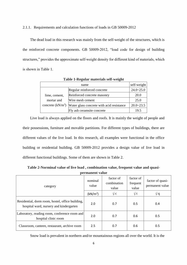
2.1.1. Requirements and calculation functions of loads in GB 50009-2012

The dead load in this research was mainly from the self-weight of the structures, which is

the reinforced concrete components. GB 50009-2012, “load code for design of building

structures,” provides the approximate self-weight density for different kind of materials, which

is shown in Table 1.

Table 1-Regular materials self-weight

name self-weight

lime, cement,

mortar and

concrete (kN/m3)

Regular reinforced concrete 24.0~25.0

Reinforced concrete masonry 20.0

Wire mesh cement 25.0

Water glass concrete with acid resistance 20.0~23.5

Fly ash ceramsite concrete 19.5

Live load is always applied on the floors and roofs. It is mainly the weight of people and

their possessions, furniture and movable partitions. For different types of buildings, there are

different values of the live load. In this research, all examples were functional in the office

building or residential building. GB 50009-2012 provides a design value of live load in

different functional buildings. Some of them are shown in Table 2.

Table 2-Norminal value of live load , combination value, frequent value and quasi-

permanent value

category

nominal

value

factor of

combination

value

factor of

frequent

value

factor of quasi-

permanent value

(kN/m2) yc yt yq

Residential, dorm room, hostel, office building,

hospital ward, nursery and kindergarten 2.0 0.7 0.5 0.4

Laboratory, reading room, conference room and

hospital clinic room 2.0 0.7 0.6 0.5

Classroom, canteen, restaurant, archive room 2.5 0.7 0.6 0.5

Snow load is prevalent in northern and/or mountainous regions all over the world. It is the

7

result of the accumulation of snow from many storms over the course of a winter season.

Between winter storms, the roof systems may lose some of the accumulated snow as the result

of wind activity and/or melting from either warm temperatures, or from building heat (Ministry

of Housing and Urban-Rural Development of the People's Republic of China, Beijing 2012).

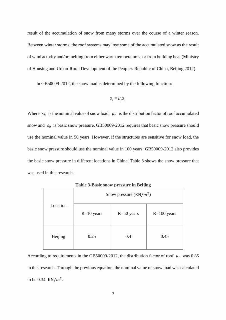
In GB50009-2012, the snow load is determined by the following function:

0ss rk =

Where 𝑠𝑘 is the nominal value of snow load, 𝜇𝑟 is the distribution factor of roof accumulated

snow and 𝑠0 is basic snow pressure. GB50009-2012 requires that basic snow pressure should

use the nominal value in 50 years. However, if the structures are sensitive for snow load, the

basic snow pressure should use the nominal value in 100 years. GB50009-2012 also provides

the basic snow pressure in different locations in China, Table 3 shows the snow pressure that

was used in this research.

Table 3-Basic snow pressure in Beijing

Location

Snow pressure (KN/𝑚2)

R=10 years R=50 years R=100 years

Beijing 0.25 0.4 0.45

According to requirements in the GB50009-2012, the distribution factor of roof 𝜇𝑟 was 0.85

in this research. Through the previous equation, the nominal value of snow load was calculated

to be 0.34 KN/𝑚2.

8

Wind is a mass of air that moves in a mostly horizontal direction from an area of high

pressure to an area with low pressure (J. Struct. Eng., 1999, 125(4): 453-463). High winds

can be very destructive because they generate pressure against the surface of a structure. The

intensity of this pressure is the wind load. The effect of the wind is dependent upon the size

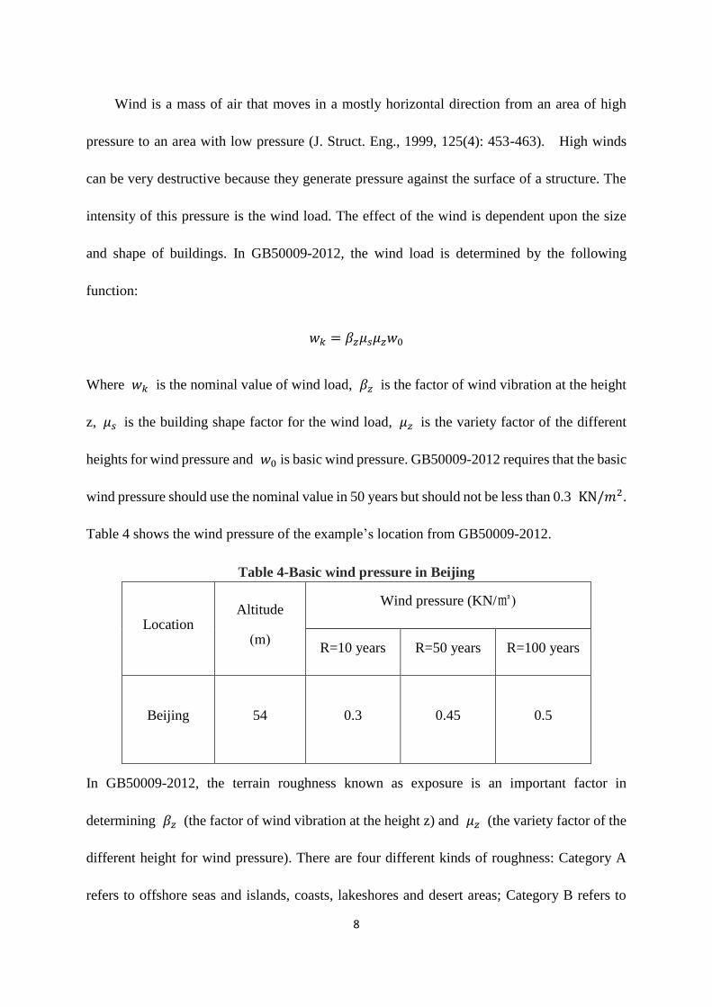
and shape of buildings. In GB50009-2012, the wind load is determined by the following

function:

𝑤𝑘 = 𝛽𝑧𝜇𝑠𝜇𝑧𝑤0

Where 𝑤𝑘 is the nominal value of wind load, 𝛽𝑧 is the factor of wind vibration at the height

z, 𝜇𝑠 is the building shape factor for the wind load, 𝜇𝑧 is the variety factor of the different

heights for wind pressure and 𝑤0 is basic wind pressure. GB50009-2012 requires that the basic

wind pressure should use the nominal value in 50 years but should not be less than 0.3 KN/𝑚2.

Table 4 shows the wind pressure of the example’s location from GB50009-2012.

Table 4-Basic wind pressure in Beijing

Location Altitude

(m)

Wind pressure (KN/㎡)

R=10 years R=50 years R=100 years

Beijing 54 0.3 0.45 0.5

In GB50009-2012, the terrain roughness known as exposure is an important factor in

determining 𝛽𝑧 (the factor of wind vibration at the height z) and 𝜇𝑧 (the variety factor of the

different height for wind pressure). There are four different kinds of roughness: Category A

refers to offshore seas and islands, coasts, lakeshores and desert areas; Category B refers to

9

fields, villages, jungles, hills, and townships where housing is sparse; Category C refers to

urban areas of densely populated clusters; Category D refers to cities with dense buildings and

high-rising buildings in urban areas. In this research, the roughness was classified as Category

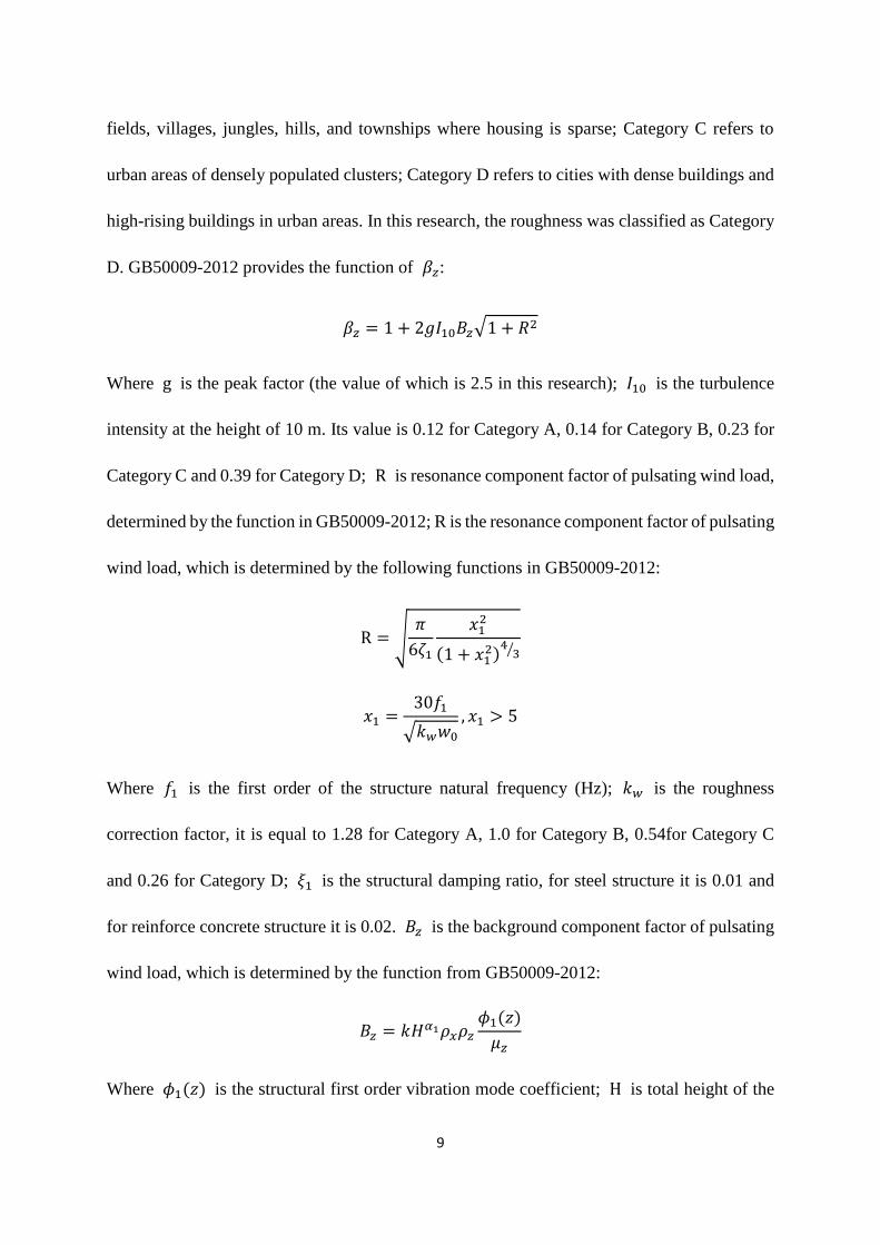
D. GB50009-2012 provides the function of 𝛽𝑧:

𝛽𝑧 = 1 + 2𝑔𝐼10𝐵𝑧√1 + 𝑅2

Where g is the peak factor (the value of which is 2.5 in this research); 𝐼10 is the turbulence

intensity at the height of 10 m. Its value is 0.12 for Category A, 0.14 for Category B, 0.23 for

Category C and 0.39 for Category D; R is resonance component factor of pulsating wind load,

determined by the function in GB50009-2012; R is the resonance component factor of pulsating

wind load, which is determined by the following functions in GB50009-2012:

R = √𝜋

6𝜁1

𝑥12

(1 + 𝑥12)

43⁄

𝑥1 =30𝑓1

√𝑘𝑤𝑤0

, 𝑥1 > 5

Where 𝑓1 is the first order of the structure natural frequency (Hz); 𝑘𝑤 is the roughness

correction factor, it is equal to 1.28 for Category A, 1.0 for Category B, 0.54for Category C

and 0.26 for Category D; 𝜉1 is the structural damping ratio, for steel structure it is 0.01 and

for reinforce concrete structure it is 0.02. 𝐵𝑧 is the background component factor of pulsating

wind load, which is determined by the function from GB50009-2012:

𝐵𝑧 = 𝑘𝐻𝛼1𝜌𝑥𝜌𝑧

𝜙1(𝑧)

𝜇𝑧

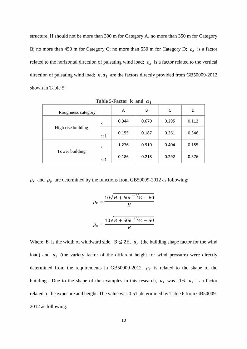
Where 𝜙1(𝑧) is the structural first order vibration mode coefficient; H is total height of the

10

structure, H should not be more than 300 m for Category A, no more than 350 m for Category

B; no more than 450 m for Category C; no more than 550 m for Category D; 𝜌𝑥 is a factor

related to the horizontal direction of pulsating wind load; 𝜌𝑧 is a factor related to the vertical

direction of pulsating wind load; 𝑘, 𝛼1 are the factors directly provided from GB50009-2012

shown in Table 5;

Table 5-Factor 𝐤 and 𝜶𝟏

Roughness category A B C D

High rise building k 0.944 0.670 0.295 0.112

a1 0.155 0.187 0.261 0.346

Tower building k 1.276 0.910 0.404 0.155

a1 0.186 0.218 0.292 0.376

𝜌𝑥 and 𝜌𝑦 are determined by the functions from GB50009-2012 as following:

𝜌𝑧 =10√𝐻 + 60𝑒

−𝐻60⁄ − 60

𝐻

𝜌𝑥 =10√𝐵 + 50𝑒

−𝐻60⁄ − 50

𝐵

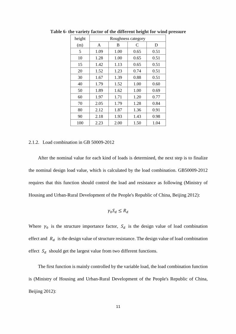
Where B is the width of windward side, B ≤ 2H. 𝜇𝑠 (the building shape factor for the wind

load) and 𝜇𝑧 (the variety factor of the different height for wind pressure) were directly

determined from the requirements in GB50009-2012. 𝜇𝑠 is related to the shape of the

buildings. Due to the shape of the examples in this research, 𝜇𝑠 was -0.6. 𝜇𝑧 is a factor

related to the exposure and height. The value was 0.51, determined by Table 6 from GB50009-

2012 as following:

11

Table 6- the variety factor of the different height for wind pressure

height Roughness category

(m) A B C D

5 1.09 1.00 0.65 0.51

10 1.28 1.00 0.65 0.51

15 1.42 1.13 0.65 0.51

20 1.52 1.23 0.74 0.51

30 1.67 1.39 0.88 0.51

40 1.79 1.52 1.00 0.60

50 1.89 1.62 1.00 0.69

60 1.97 1.71 1.20 0.77

70 2.05 1.79 1.28 0.84

80 2.12 1.87 1.36 0.91

90 2.18 1.93 1.43 0.98

100 2.23 2.00 1.50 1.04

2.1.2. Load combination in GB 50009-2012

After the nominal value for each kind of loads is determined, the next step is to finalize

the nominal design load value, which is calculated by the load combination. GB50009-2012

requires that this function should control the load and resistance as following (Ministry of

Housing and Urban-Rural Development of the People's Republic of China, Beijing 2012):

𝛾0𝑆𝑑 ≤ 𝑅𝑑

Where 𝛾0 is the structure importance factor, 𝑆𝑑 is the design value of load combination

effect and 𝑅𝑑 is the design value of structure resistance. The design value of load combination

effect 𝑆𝑑 should get the largest value from two different functions.

The first function is mainly controlled by the variable load, the load combination function

is (Ministry of Housing and Urban-Rural Development of the People's Republic of China,

Beijing 2012):

12

𝑆𝑑 = ∑ 𝛾𝐺𝑗

𝑚

𝑗=1

𝑆𝐺𝑗𝑘 + 𝛾𝑄1𝛾𝐿1

𝑆𝑄1𝑘 + ∑ 𝛾𝑄𝑖

𝑛

1=2

𝛾𝐿𝑖𝜓𝑐𝑖

𝑆𝑄𝑖𝑘

Where 𝛾𝐺𝑗 is the j-th bias factor of the permanent load, 𝛾𝑄𝑖

is the i-th bias factor of the variable

load, 𝛾𝑄1is the factor for the mainly controlled variable load, 𝛾𝐿𝑖

is the i-th bias factor of the

service life considered by the variable load, 𝛾𝐿1 is the factor for the mainly controlled variable

load, 𝑆𝐺𝑗𝑘 is the j-th the nominal value of the load effect of the permanent load, 𝑆𝑄𝑖𝑘 is the

i-th the nominal value of the load effect of the variable load, 𝜓𝑐𝑖is the i-th combination factor

of variable load 𝑄𝑖, 𝑚 is the quantity of the permanent load and 𝑛 is the quantity of the

variable load;

The second function is mainly controlled by permanent load, the load combination

function is (Ministry of Housing and Urban-Rural Development of the People's Republic of

China, Beijing 2012):

𝑆𝑑 = ∑ 𝛾𝐺𝑗

𝑚

𝑗=1

𝑆𝐺𝑗𝑘 + ∑ 𝛾𝑄𝑖

𝑛

1=2

𝛾𝐿𝑖𝜓𝑐𝑖

𝑆𝑄𝑖𝑘

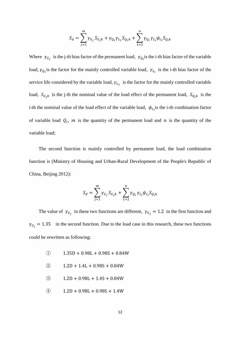
The value of 𝛾𝐺𝑗 in these two functions are different, 𝛾𝐺𝑗

= 1.2 in the first function and

𝛾𝐺𝑗= 1.35 in the second function. Due to the load case in this research, these two functions

could be rewritten as following:

① 1.35D + 0.98L + 0.98S + 0.84W

② 1.2D + 1.4L + 0.98S + 0.84W

③ 1.2D + 0.98L + 1.4S + 0.84W

④ 1.2D + 0.98L + 0.98S + 1.4W

13

Through load combination, load effect 𝑞𝑢 could be estimated. Once 𝑞𝑢 is determined,

the required resistance would be calculated through the LRFD (Loads and Resistance Factor

Design) method.

2.1.3. Statistical parameters of loads in GB5009-2012

The reliability analysis requires the statistical data for each factor in the limit state function.

Therefore, the statistical parameters of loads are necessary to analyze. Because of the different

code’s requirements, the statistical datas for each load in GB50010-2010 are not the same as

they are in ASCE 7-10.

This research contained dead load, live load, wind load and snow load as the forces applied

to the examples. Dead load is a constant load, unlike the live load, wind load and snow load,

in that dead load does not change along the service life. The statistic parameter of dead load

was presented by Zhenchang Li and Jiayan Wang，1986. Generally, live load has a significant

influence on the reliability analysis. In GB50009-2012, the statistical survey results for live

load separates into two kinds of live loads: constant live load and temporary live load. The

constant live load is considered to be an invariable live load in a certain period, such as the

load from furniture. The temporary live load is supposed to be a live load occasionally applied

in a short term, such as the human weight in a party. GB50009-2012 presents the statistical

parameters for these two kinds of live loads. The statistical parameter of snow load, which is

based on the meteorological data, was presented by Bonian Hou and Caiang Wei，1986. Wind

load is also based on meteorological data, the statistic parameter of wind load was presented

by Xiangyuan Tu，1986. The summary of statistical parameters of loads is shown in Table 7.

14

Table 7- Statistical parameter of loads in GB5009-2012

Load type Bias

factor COV Distribution type

Dead 1.06 0.07 normal

Constant live 0.193 0.4611 extreme 1

Temporary Live 0.1775 0.6873 extreme 1

Wind 0.610 0.27 extreme 1

Snow 0.358 0.712 extreme 1

2.2. Load design methods and requirements in American code (ASCE 7-10)

For the comparison, the examples designed by American codes applied the same kinds of

loads: dead load, live load, snow load and wind load. ASCE 7-10 provides the detailed

requirements and calculation functions for each load, which are quite different from those

provided from GB50009-2012.

2.2.1. Requirements and calculation functions of loads in ASCE 7-10

“Dead Loads consist of the weight of all materials of construction incorporated into the

building including, but not limited to, walls, floors, roofs, ceilings, stairways, built-in partitions,

finishes, cladding, and other similarly incorporated architectural and structural items and fixed

service equipment including the weight of cranes” (ASCE 7-10, Reston, 2010). The definition

of dead load in ASCE 7 is similar to the description in GB50009-2012. Due to the comparison,

each couple of examples kept the same dimensions and materials. Therefore, the dead load of

the examples designed by ASCE 7-10 was also the self-weight of the reinforced concrete

15

components. The approximate unit weight of reinforced concrete for design is 150 pcf , which

is equal to 24 KN/𝑚3.

In ASCE 7-10, there are several types of loads considered to be live load. It includes: fixed

ladder, grab bar system, guardrail system, handrail system, helipad, live load, roof live load,

screen enclosure and vehicle barrier system (ASCE 7-10, 2010). In this research, live load was

the typical live load, usually “produced by the use and occupancy of the building or other

structure that does not include construction or environmental loads” (ASCE 7-10, 2010). ASCE

7 -10 provides a design live load 2.4 KN/𝑚2 for an office building, which is larger than the

value in the Chinese code.

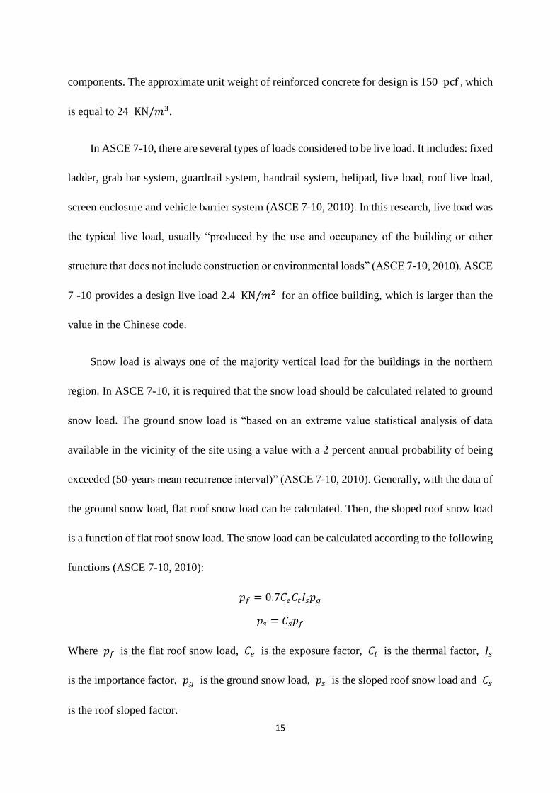
Snow load is always one of the majority vertical load for the buildings in the northern

region. In ASCE 7-10, it is required that the snow load should be calculated related to ground

snow load. The ground snow load is “based on an extreme value statistical analysis of data

available in the vicinity of the site using a value with a 2 percent annual probability of being

exceeded (50-years mean recurrence interval)” (ASCE 7-10, 2010). Generally, with the data of

the ground snow load, flat roof snow load can be calculated. Then, the sloped roof snow load

is a function of flat roof snow load. The snow load can be calculated according to the following

functions (ASCE 7-10, 2010):

𝑝𝑓 = 0.7𝐶𝑒𝐶𝑡𝐼𝑠𝑝𝑔

𝑝𝑠 = 𝐶𝑠𝑝𝑓

Where 𝑝𝑓 is the flat roof snow load, 𝐶𝑒 is the exposure factor, 𝐶𝑡 is the thermal factor, 𝐼𝑠

is the importance factor, 𝑝𝑔 is the ground snow load, 𝑝𝑠 is the sloped roof snow load and 𝐶𝑠

is the roof sloped factor.

16

In ASCE 7-10, the wind load calculations are separated into two types. One is applied to

main wind force resisting systems; another is applied to components and claddings. In this

research, beams and columns were the main research objects. They were part of the main wind

force resisting system. There are several methods to calculate wind load. The envelope

procedure was selected to be the calculation method here, which is specified to low rise

buildings. The wind pressure can be calculated according to the following function (ASCE 7-

10, 2010):

p = 𝑞ℎ[(𝐺𝐶𝑝𝑓) − (𝐺𝐶𝑝𝑖)]

Where p is the design wind pressure, 𝑞ℎ is the velocity pressure evaluated at mean roof

height, 𝐺𝐶𝑝𝑓 is the external pressure coefficient and 𝐺𝐶𝑝𝑖 is the internal pressure coefficient.

2.2.2. Load Combination in ASCE 7-10

Load combination is the most important step to determine the load effect on the structure.

Just like GB50010-2010, ASCE 7-10 also followed the LRFD method to proceed design.

However, even both codes used the load combination to figure out the total load effect, the

exact combination functions are not the same. In ASCE 7-10 chapter 2, the basic load

combinations are given:

① 1.4D

② 1.2D + 1.6L + 0.5(𝐿𝑟 𝑜𝑟 𝑆 𝑜𝑟 𝑅)

③ 1.2D + 1.6(𝐿𝑟 𝑜𝑟 𝑆 𝑜𝑟 𝑅) + (𝐿 𝑜𝑟 0.5𝑊)

④ 1.2D + 1.0W + L + 0.5(𝐿𝑟 𝑜𝑟 𝑆 𝑜𝑟 𝑅)

⑤ 1.2D + 1.0E + L + 0.2S

17

⑥ 0.9D+1.0W

⑦ 0.9D+1.0E

Load effect 𝑞𝑢 is the largest value throughout the previous load combinations. Once 𝑞𝑢 is

determined, the required resistance is gained by factored 𝑞𝑢.

2.2.3. Statistical parameters of loads in ASCE 7-10

In this research, all the examples show later to meet the requirements in ASCE 7-10 and

cooperated with ACI318-14. The design load（ factored load）was defined by the load

combination in chapter 2.2.2. Here, it contained dead load, live load, wind load and snow load.

Unlike GB 50010-2010, live load does not separate into two individual categories. The

statistical parameter of dead load was obtained from F.M. Bartlett, H.P. Hong, and W. Zhou,

Can, 2003. The statistical parameter of live load was obtained from Nowak, A.S. and Collins,

K.R, CRC Press,2013. The statistical parameter of wind load was obtained from Bruce R.

Ellingwood and Paulos Beraki Tekie, 1999. The statistical parameter of snow load was

obtained from Kyung Ho Lee and David V. Rosowsky, 2005. The summary of loads statistical

parameters is shown in Table 8.

Table 8- Statistical parameter of loads in ASCE 7-10

Load type Bias factor COV Distribution type

Dead 1.05 0.1 normal

Live 0.273 0.598 extreme 1

Wind 0.66 0.37 extreme 1

Snow 0.224 0.82 lognormal

18

3. Resistance of reinforced concrete beam

Generally, beams will resist loads from the floor or roof, primarily in flexure load. This

research will focus on the beam moment resistance. The requirements in Chinese code GB

50010-2010 and American code ACI 318-14 are similar. The only difference is the equivalent

rectangular concrete stress.

3.1. Beam resistance design method in GB 50010-2010

The example was a simple supported beam, which is considered as resisting positive

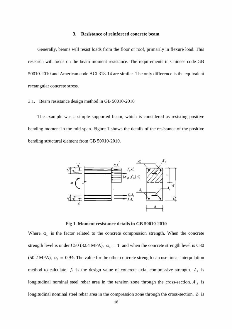
bending moment in the mid-span. Figure 1 shows the details of the resistance of the positive

bending structural element from GB 50010-2010.

Fig 1. Moment resistance details in GB 50010-2010

Where α1 is the factor related to the concrete compression strength. When the concrete

strength level is under C50 (32.4 MPA), α1 = 1 and when the concrete strength level is C80

(50.2 MPA), α1 = 0.94. The value for the other concrete strength can use linear interpolation

method to calculate. 𝑓𝑐 is the design value of concrete axial compressive strength. 𝐴𝑠 is

longitudinal nominal steel rebar area in the tension zone through the cross-section. 𝐴′𝑠 is

longitudinal nominal steel rebar area in the compression zone through the cross-section. 𝑏 is

19

the width of the rectangular cross-section. h0 is the effective height of the section. a′s is the

distance between the edge to the total force point of regular bars in the compression zone. x

is the height of the concrete compression block, 2a′ ≤ x ≤ 𝜉𝑏ℎ0. a′ is the distance between

the edge to the total force point of all reinforcements in the compression zone. 𝜉𝑏 is the

relative limit pressure zone height. Because there were no prestressed rebar or wires and no

reinforcement to resist negative moment, the resistance function could be rewritten as

following:

M ≤ 𝛼1𝑓𝑐𝑏𝑥 (ℎ0 −𝑥

2)

𝛼1𝑓𝑐𝑏𝑥 = 𝑓𝑦𝐴𝑠

This function provided by GB 50010-2010 is the beam resistance function. The reinforcement

area of the cross-section can be calculated from this function. Afterward, this resistance

function can be used for reliability analysis.

3.2. Beam resistance design method in ACI 318-14

Due to the same assumption and principle for beam design, the moment resistance

function of the beam was similar. Because there was only positive reinforcement in the beam

examples, the resistance function for a simple supported beam could be calculated by the

following function:

R = 𝐴𝑠𝑓𝑦 (𝑑 −𝑎

2)

a =𝐴𝑠𝑓𝑦

𝛽1𝑓′𝑐𝑏

The details of the positive moment resistance are shown in Figure 2.

20

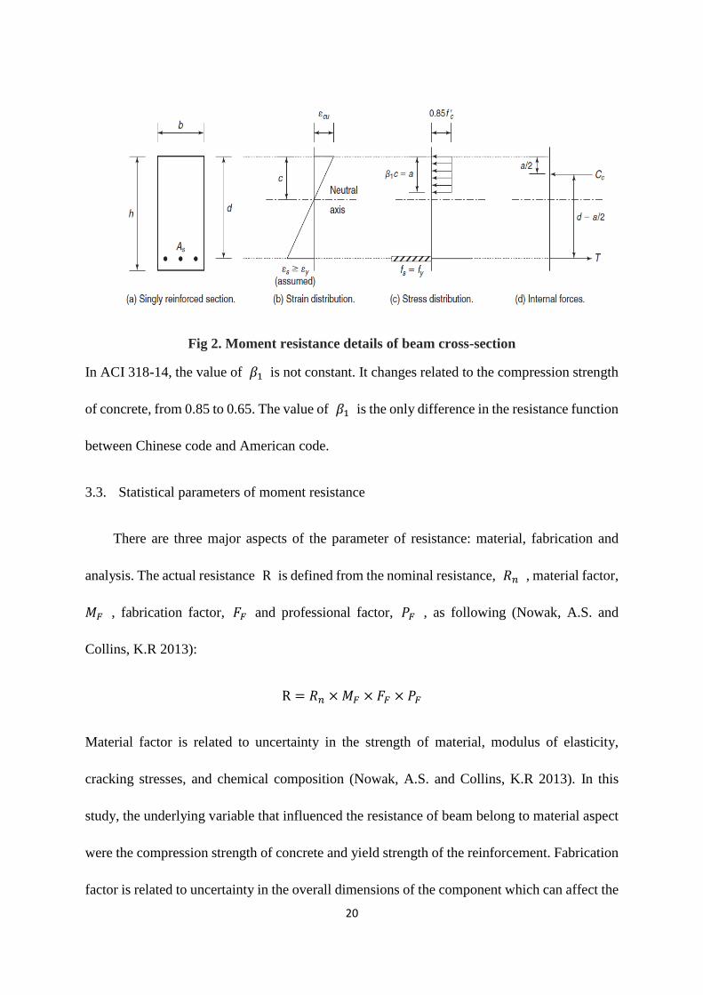
Fig 2. Moment resistance details of beam cross-section

In ACI 318-14, the value of 𝛽1 is not constant. It changes related to the compression strength

of concrete, from 0.85 to 0.65. The value of 𝛽1 is the only difference in the resistance function

between Chinese code and American code.

3.3. Statistical parameters of moment resistance

There are three major aspects of the parameter of resistance: material, fabrication and

analysis. The actual resistance R is defined from the nominal resistance, 𝑅𝑛 , material factor,

𝑀𝐹 , fabrication factor, 𝐹𝐹 and professional factor, 𝑃𝐹 , as following (Nowak, A.S. and

Collins, K.R 2013):

R = 𝑅𝑛 × 𝑀𝐹 × 𝐹𝐹 × 𝑃𝐹

Material factor is related to uncertainty in the strength of material, modulus of elasticity,

cracking stresses, and chemical composition (Nowak, A.S. and Collins, K.R 2013). In this

study, the underlying variable that influenced the resistance of beam belong to material aspect

were the compression strength of concrete and yield strength of the reinforcement. Fabrication

factor is related to uncertainty in the overall dimensions of the component which can affect the

21

cross-section area, moment of inertia and section modulus (Nowak, A.S. and Collins, K.R

2013). The primary variable that influenced the resistance of beam belong to the fabrication

factor were dimensions of the cross-section here. Professional factor is related to uncertainty

resulting from approximate methods of analysis and idealized stress/strain distribution models

(Nowak, A.S. and Collins, K.R 2013). In GB 50010-2010 and ACI 318-14, the principle of

moment resistance function is almost the same. However, the statistic parameters of the

material factors, fabrication factors and professional factors are not the same. The summary of

moment resistance statistical parameters of GB 50010-2010 is shown in Table 9 (Xinyan Shao,

Chongxi Bai, Wang Liang, Atlantis Press, 2015).

Table 9- Statistical parameters of moment resistance in GB 50010-2010

parameter nominal bias

factor COV distribution type

𝑓𝑐 20.1 MPa 1.41 0.19 normal

𝑓𝑦 400 MPa 1.12 0.093 normal

ρ 0.0045-0.01 1 0.05 normal

b 300 mm 1 0.02 normal

h 800 mm 1 0.02 normal

d 760 mm 1 0.03 normal

The summary of moment resistance statistical parameters of ACI 318-14 is shown in

Table 10 (Andrzej S. Nowak and Maria M. Szerszen, Boca Raton, 2013).

22

Table 10- Statistical parameters of moment resistance in ACI 318-14

parameter nominal bias factor COV distribution

type

𝑓′𝑐 20.6 MPa 1.25 0.135 normal

𝑓𝑦 413.67 MPa 1.2-1.125 0.057 normal

ρ 0.0045-0.01 1 0.049 normal

b 300 mm 1.01 0.04 normal

h 800 mm 1.01 0.04 normal

d 760 mm 0.99 0.04 normal

The ultimate strength of the beam would vary due to the factors showed in Table 9 and Table

10. With the moment resistance function, the actual resistance for reliability analysis can be

calculated.

23

4. Resistance of reinforced concrete column

Column is one important element of the load resistance structural system. Rather than the

simply supported beam, the column mainly resists the bending moment and axial force

simultaneously. It is also required to resist torsion and shear. The design and analysis of

columns are more complicated than the simple supported beam. The design procedure of

columns is similar as beams. At first, the load combination estimates required resistance, then

the reinforcement can be calculated by the functions from the code. In the Chinese codes, the

column separates into two categories: large eccentric compression member and small eccentric

compression member. These two kinds of column design methods have different requirements

and design procedure, which will be introduced carefully in the following paragraph. In

American codes (ACI 318), the column design separates as two methods: non-sway frame

column design and sway frame column design. Determination of sway frame and non-sway

frame depends on the rigidness of whole frame structures. Due to each code having different

categories in the column design methods, this research generated six basic calculation examples

for comparison. In addition, the design requirements of loads are the same as chapter two.

4.1. Column resistance design method in ACI 318

In GB 50010-2010, columns are considered as a structural member that resists moment

and axial force in tandem. There are two types of column: large eccentric compression member

and small eccentric compression member. Each of them has different design methods.

Before estimating the column type, it should verify the slenderness effect on the design

moment. If 𝑙𝑐 𝑖⁄ ≤ 34 − 12(𝑀1/𝑀2) , the slenderness effect could be neglected; if not, the

24

influence of the slenderness effect on the design requirement moment should be considered.

With the slenderness effect, the design requirement moment should be enlarged. It could be

replaced by M, which could be expressed by:

M = 𝐶𝑚𝜂𝑛𝑠𝑀2

𝐶𝑚 = 0.7 + 0.3𝑀1

𝑀2≥ 0.7

𝜂𝑛𝑠 = 1 +1

1300 (𝑀2

𝑁 + 𝑒𝑎) ℎ0⁄(

𝑙𝑐

ℎ)

2

𝜁𝑐

𝜁𝑐 =0.5𝑓𝑐𝐴

𝑁

Where N is the design axial force due to 𝑀2; 𝑒𝑎 is the additional eccentricity, which is the

larger value between 20 mm and 1/30 of cross-section height; A is the gross area of the cross-

section;

After the required moment resistance enlarged due to slenderness, the columns should be

verified as large eccentric compression members or small eccentric compression members. The

central principle to verify the column types is to compare the factored eccentricity with the

0.3ℎ0, where ℎ0 is the distance from the edge of the compression block in the cross-section

to the edge of longitude steel rebar in the tension zone. If the factored eccentricity is larger than

0.3ℎ0, the design column should be considered as a large eccentric compression member; if

not, it should be considered as a small eccentric compression member. According to GB 50010-

2010, the factored eccentricity has two components: eccentricity enlarge factor, η, and initial

eccentricity, 𝑒𝑖. The initial eccentricity, 𝑒𝑖, could be expressed by

𝑒𝑖 = 𝑒0 + 𝑒𝑎

25

Where 𝑒0 is the design eccentricity, which could be expressed by

𝑒0 =𝑀𝑢

𝑃𝑢

Where 𝑀𝑢 is the design moment requirement; 𝑃𝑢 is the design axial force requirement; 𝑒𝑎

is the additional eccentricity, which is the larger value between 20 mm and 1/30 of cross-section

height. The eccentricity enlarge factor, η, could be expressed by

η = 1 +1

1400𝑒𝑖 ℎ0⁄(

𝑙0

ℎ)

2

𝜁1𝜁2

Where, 𝑙0 is the effective length of the compression member; h is the total height of cross-

section; 𝜁1 is the correction factor for the eccentric compression member curvature, which

could be expressed by

𝜁1 =0.5𝑓𝑐𝐴

𝑃𝑢

Where 𝜁2 is the slenderness effect factor, which could be expressed by

𝜁2 = 1.15 − 0.01𝑙0

ℎ

So, if the design column is estimated as a large eccentric compression member, the next

step is to calculate required reinforcement by the functions in the codes. Because of the axial

force, when the column achieves the limit state, the reinforcement in the tension area does not

always achieve yield strength. That means the moment capacity is related to the axial force

capacity, which cannot be considered separately. The limit state of the column is either moment

or axial force achieving the ultimate strength. In GB 50010-2010, the ultimate compression

strain in concrete is defined as, 𝜀𝑐𝑢 , which can be calculated by 𝜀𝑐𝑢 = 0.0033 −

26

(𝑓𝑐 − 50) × 10−5 . With the ultimate compression strain in concrete and the stress-strain

relationship, the stress of reinforcement in the ultimate strength could be calculated. In addition,

the strength capacity functions of columns are the combination of reinforcement contribution

and concrete contribution. The height of the concrete compression block, x, is important to

determine the stress of the reinforcement in the limit state. Once x is known, the strain of any

heights through the cross-section could be calculated by using 𝜀𝑐𝑢 and the linear stress-strain

relationship. GB 50010-2010 illustrates that the limit state of the large eccentric compression

column is the reinforcement in the tension zone achieving yield strength and the concrete in

the compression zone achieving the ultimate compression strain 𝜀𝑐𝑢 concurrently. GB 50010-

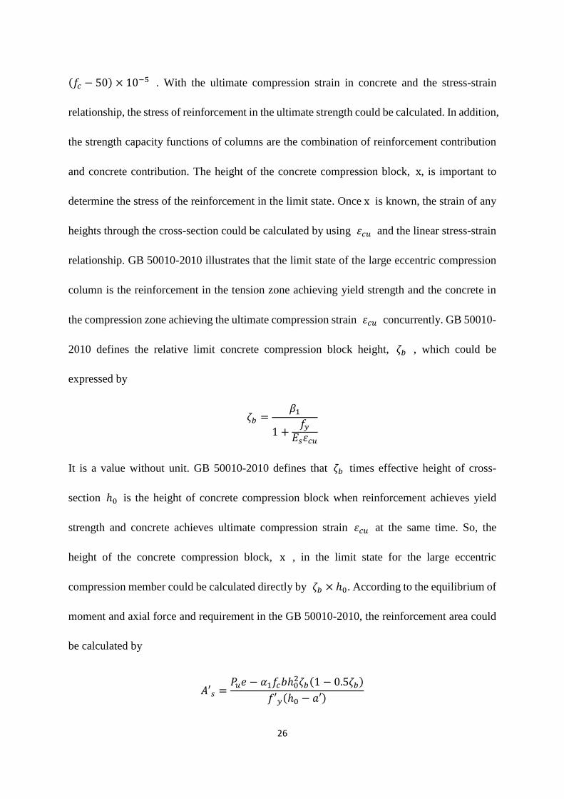
2010 defines the relative limit concrete compression block height, 𝜁𝑏 , which could be

expressed by

𝜁𝑏 =𝛽1

1 +𝑓𝑦

𝐸𝑠𝜀𝑐𝑢

It is a value without unit. GB 50010-2010 defines that 𝜁𝑏 times effective height of cross-

section ℎ0 is the height of concrete compression block when reinforcement achieves yield

strength and concrete achieves ultimate compression strain 𝜀𝑐𝑢 at the same time. So, the

height of the concrete compression block, x , in the limit state for the large eccentric

compression member could be calculated directly by 𝜁𝑏 × ℎ0. According to the equilibrium of

moment and axial force and requirement in the GB 50010-2010, the reinforcement area could

be calculated by

𝐴′𝑠 =𝑃𝑢𝑒 − 𝛼1𝑓𝑐𝑏ℎ0

2𝜁𝑏(1 − 0.5𝜁𝑏)

𝑓′𝑦(ℎ0 − 𝑎′)

27

e = η𝑒𝑖 +ℎ

2− 𝑎

𝐴𝑠 =𝛼1𝑓𝑐𝑏ℎ0𝜁𝑏 + 𝑓′𝑦𝐴′𝑠 − 𝑃𝑢

𝑓𝑦

Where a′ is the distance from the neutral axis of reinforcement in compression zone to the

edge of the concrete compression block; a is the distance from the neutral axis of

reinforcement in the tension zone to the edge of the concrete. In addition, GB 50010-2010

requires that the reinforcement ratio in the compression zone should not be less than 0.2%; the

reinforcement ratio in the tension zone should not be less than 0.2%; the total reinforcement

ratio should not be less than 0.6%. It also requires checking the compression resistance, which

could be expressed by

𝑃𝑢 = 0.9𝜑(𝑓𝑐𝐴 + 𝑓′𝑦𝐴′𝑠)

Where 𝜑 is the stability factor of the column, which is related to the length of member and

width of the cross-section.

If the design column estimates as small eccentric compression member, there are two steps

to verify the column eccentric type. The first step is the same method to verify the eccentric

column type as large eccentric compression member, to compare the factored eccentricity η𝑒𝑖

with the 0.3ℎ0, If η𝑒𝑖 is larger than 0.3ℎ0, the design column should be considered as large

eccentric compression member. If η𝑒𝑖 is less than 0.3ℎ0, it could be possible small eccentric

compression member. The second step is to assume that the member is small eccentric

compression column, and then calculate the relative height of compression concrete block, ζ .

GB 50010-2010 provided the function of ζ specific for small eccentric compression member,

28

which could be expressed by

ζ =𝑃𝑢 − 𝜁𝑏𝛼1𝑓𝑐𝑏ℎ0

𝑃𝑢𝑒 − 0.43𝛼1𝑓𝑐𝑏ℎ02

(𝛽1 − 𝜁𝑏)(ℎ0 − 𝑎′𝑠)+ 𝛼1𝑓𝑐𝑏ℎ0

+ 𝜁𝑏

e = η𝑒𝑖 +ℎ

2− 𝑎

If ζ > 𝜁𝑏 , the column could be considered as small eccentric compression member. If not, the

column should follow the rules of large eccentric compression member. So once the design

column is defined as small eccentric compression member, the next step should also be to

calculate required reinforcement. For the purpose to calculate reinforcement, the limit state is

the key to determine the functions, which is quite different between large eccentric

compression member and small eccentric compression member. The limit state of large

eccentric compression member is that the reinforcement in tension zone is yield and concrete

strain achieves limit height of compression block in the same time. But for the small eccentric

compression member, when the member achieves the axial force capacity, the reinforcement

in the tension zone could not achieve the yield strength. That requires to calculate the stress of

reinforcement in the tension zone in the limit state, which would not be equal to 𝑓𝑦 . It is back

to the same procedure as large eccentric compression member; calculate the height of the

concrete compression block, x, then calculate strain of reinforcement in the tension zone by

using stress-strain relationship and 𝜀𝑐𝑢 . But GB 50010-2010 provides the approximate

functions to calculate reinforcement area for small eccentric compression member if 𝐴𝑠 = 𝐴′𝑠

(reinforcement area in the tension zone is equal to the reinforcement area in the compression

zone), it could be expressed by

29

𝐴𝑠 = 𝐴′𝑠 =𝑃𝑢 − 𝜁(1 − 0.5𝜁)𝛼1𝑓𝑐𝑏ℎ0

2

𝑓′𝑦(ℎ0 − 𝑎′𝑠)

Where the relative height of compression concrete block, ζ should be calculated when column

eccentric types were verified. After estimating the reinforcement, GB 50010-2010 requires to

check minimum reinforcement ratio and the compression resistance, which is as same as large

eccentric compression member.

4.2. Column resistance design method in GB 50010-2010

There are two types of design method in ACI 318-14: sway frame design and non-sway

frame design. For the purpose to verify the sway or non-sway fame, stability index, Q, should

be calculated first, which could be expressed by

Q =∑ 𝑃𝑢 Δ0

𝑉𝑢𝑠𝑙𝑐

Where ∑ 𝑃𝑢 is total vertical load in the story corresponding to the lateral loading case; 𝑉𝑢𝑠 is

factored story shear in the story corresponding to the lateral loading case; Δ0 is first-order

relative lateral deflection between top and bottom of the story due to 𝑉𝑢𝑠. If Q < 0.05 , this

story level should be considered as a non-sway frame. If not, it should be consider as a sway

frame.

Generally, the column design requires the all detailed loads and deflection analysis, which

is quite different from GB 50010-2010. In addition, the stability index should be calculated due

to each load combination provided in the ASCE 7-10. If there is anyone combination making

the stability index, Q, exceed 0.05, this story should be considered as a sway frame.

A non-sway frame is the structure with small interstorey displacements. Once the design

30

column’s story level is estimated as a non-sway frame, the next step is to verify the slenderness

effect could be neglected or not. In ACI 318-14, for columns not braced against sidesway, if

k𝑙𝑢 𝑟⁄ ≤ 22 , the slenderness effect could be neglected; for columns braced against sidesway,

if k𝑙𝑢 𝑟⁄ ≤ 34 + 12(𝑀1 𝑀2⁄ ) and k𝑙𝑢 𝑟⁄ ≤ 40 , the slenderness effect could be neglected. If

the slenderness could be neglected, the column design should follow first-order analysis. If the

slenderness effect could not be neglected, the column design should consider the slenderness

effect through the column length, using the second order analysis. If 𝑀2𝑛𝑑−𝑜𝑟𝑑𝑒𝑟 ≤

1.4𝑀1𝑠𝑡−𝑜𝑟𝑑𝑒𝑟 , then use the 𝑀2𝑛𝑑−𝑜𝑟𝑑𝑒𝑟 as required design moment. If not, the structural

system should be revised.

The sway frame is the structure capable to resist lateral loads by itself. It is not necessary

to require additional bracing for stability; therefore, the sway frame would have a larger

displacement rather than the non-sway frame. The first step for sway frame design is the same

as non-sway design: the slenderness effect could be neglected or not. If slenderness effect could

not be neglected, ACI 318-14 requires considering the slenderness effects at column ends first,

which is second-order elastic analysis. The next step is to check the slenderness effect along

the column length, which is as same as non-sway frame column. After these second-order

analyses, the next step is to calculate the critical moment 𝑀2𝑛𝑑−𝑜𝑟𝑑𝑒𝑟 , made sure

𝑀2𝑛𝑑−𝑜𝑟𝑑𝑒𝑟 ≤ 1.4𝑀1𝑠𝑡−𝑜𝑟𝑑𝑒𝑟 , used the 𝑀2𝑛𝑑−𝑜𝑟𝑑𝑒𝑟 as required design moment, otherwise

revised the structural system.

After determining the required axial force and moment resistance, they should be applied

into the column strength interaction diagram for rectangular section to find out the required

reinforcement ratio. But column strength is varied due to different axial force and moment. The

31

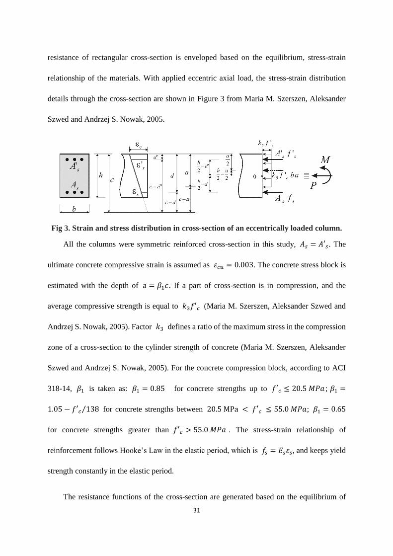
resistance of rectangular cross-section is enveloped based on the equilibrium, stress-strain

relationship of the materials. With applied eccentric axial load, the stress-strain distribution

details through the cross-section are shown in Figure 3 from Maria M. Szerszen, Aleksander

Szwed and Andrzej S. Nowak, 2005.

Fig 3. Strain and stress distribution in cross-section of an eccentrically loaded column.

All the columns were symmetric reinforced cross-section in this study, 𝐴𝑠 = 𝐴′𝑠. The

ultimate concrete compressive strain is assumed as 𝜀𝑐𝑢 = 0.003. The concrete stress block is

estimated with the depth of a = 𝛽1𝑐. If a part of cross-section is in compression, and the

average compressive strength is equal to 𝑘3𝑓′𝑐 (Maria M. Szerszen, Aleksander Szwed and

Andrzej S. Nowak, 2005). Factor 𝑘3 defines a ratio of the maximum stress in the compression

zone of a cross-section to the cylinder strength of concrete (Maria M. Szerszen, Aleksander

Szwed and Andrzej S. Nowak, 2005). For the concrete compression block, according to ACI

318-14, 𝛽1 is taken as: 𝛽1 = 0.85 for concrete strengths up to 𝑓′𝑐 ≤ 20.5 𝑀𝑃𝑎 ; 𝛽1 =

1.05 − 𝑓′𝑐 138⁄ for concrete strengths between 20.5 MPa < 𝑓′𝑐 ≤ 55.0 𝑀𝑃𝑎; 𝛽1 = 0.65

for concrete strengths greater than 𝑓′𝑐 > 55.0 𝑀𝑃𝑎 . The stress-strain relationship of

reinforcement follows Hooke’s Law in the elastic period, which is 𝑓𝑠 = 𝐸𝑠𝜀𝑠, and keeps yield

strength constantly in the elastic period.

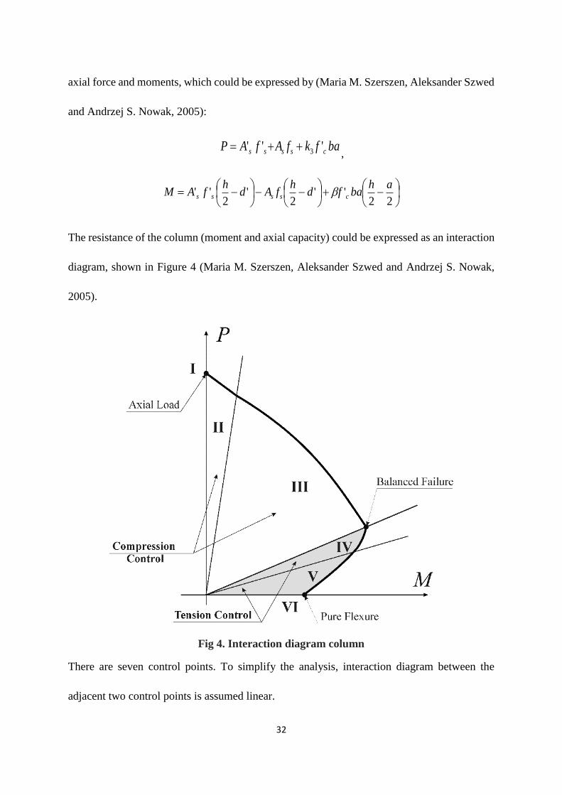
The resistance functions of the cross-section are generated based on the equilibrium of

32

axial force and moments, which could be expressed by (Maria M. Szerszen, Aleksander Szwed

and Andrzej S. Nowak, 2005):

bafkfAfAP cssss ''' 3++=,

−+

−−

−=

22''

2'

2''

ahbafd

hfAd

hfAM cssss

The resistance of the column (moment and axial capacity) could be expressed as an interaction

diagram, shown in Figure 4 (Maria M. Szerszen, Aleksander Szwed and Andrzej S. Nowak,

2005).

Fig 4. Interaction diagram column

There are seven control points. To simplify the analysis, interaction diagram between the

adjacent two control points is assumed linear.

33

① Control point 1: Pure compression

In this situation, there is no moment resistance, assume that the tension reinforcement has

no contribution to the axial force resistance, the compression reinforcement achieves the yield

strength, the resistance function could be rewritten as:

P = 0.85𝑓′𝑐(𝐴𝑔 − 𝐴′𝑠) + 𝑓′𝑦𝐴′𝑠

M = 0

② Control point 2: Bar stress near tension face equal to 0 (𝜀𝑠 = 𝑓𝑠 = 0)

In this situation, the neutral axial depth, c, is equal to the distance from the neutral axis of

tension reinforcement to the compression edge, d. Once the neutral axial depth, c, is determined,

the strain in the compression reinforcement level could be estimated by using linear stress-

strain relationship 𝜀′𝑠 = (𝑐 − 𝑑′)𝜀𝑐𝑢

𝑐. According to the extreme strain of reinforcement 𝜀𝑦 =

𝑓𝑦

𝐸𝑠 , the compression reinforcement could be estimated as yield or not, then the stress of

compression reinforcement can be calculated, 𝑓′𝑠, (𝑓′𝑠 ≤ 𝑓′𝑦). The resistance function could

be rewritten as:

𝜀′𝑠 = (𝑐 − 𝑑′)𝜀𝑐𝑢

𝑐

𝐶𝑐 = 0.85𝑓′𝑐𝑎𝑏

𝐶𝑠 = (𝑓′𝑠

− 0.85𝑓′𝑐)𝐴′𝑠

P = 𝐶𝑐 + 𝐶𝑠

M = 𝐶𝑐 (ℎ − 𝑎

2) + 𝐶𝑠 (

ℎ

2− 𝑑′)

③ Control point 3: Bar stress near tension face equal to 0.5𝑓𝑦 (𝑓𝑠 = −0.5𝑓𝑦)

34

In this situation, tension reinforcement is not yielded, but the stress is already known,

according to Hooke’s Law, the strain of the tension reinforcement is also determined by 𝜀𝑠 =

𝜀𝑦2⁄ . The neutral axial depth, c, could be calculated by using the stress-strain relationship

through the cross-section:

c =𝑑

𝜀𝑠 + 𝜀𝑐𝑢𝜀𝑐𝑢

After the neutral axial depth, c, is confirmed, the strain in the compression reinforcement level

could be calculated by the following function:


𝑐

Next is to compare 𝜀′𝑠 with 𝜀𝑦, to estimate the compression reinforcement yield or not, then

gain the stress of compression reinforcement, 𝑓′𝑠, (𝑓′𝑠 ≤ 𝑓′𝑦). The resistance function could

be rewritten as:



− 0.85𝑓′𝑐)𝐴′𝑠

𝑇𝑠 = 𝑓𝑠𝐴𝑠

P = 𝐶𝑐 + 𝐶𝑠 − 𝑇𝑠

M = 𝐶𝑐 (ℎ − 𝑎

2) + 𝐶𝑠 (

ℎ

2− 𝑑′) + 𝑇𝑠 (𝑑 −

ℎ

2)

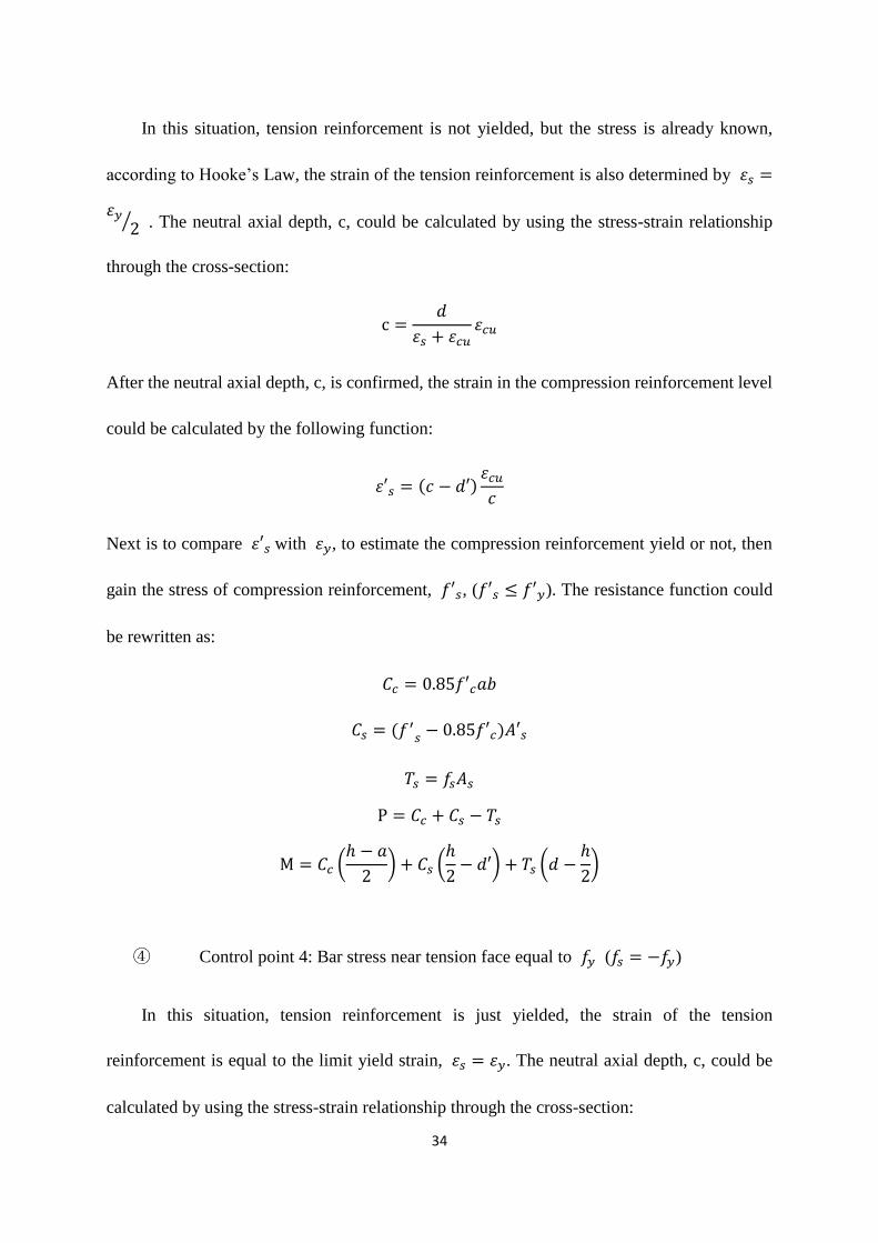
④ Control point 4: Bar stress near tension face equal to 𝑓𝑦 (𝑓𝑠 = −𝑓𝑦)

In this situation, tension reinforcement is just yielded, the strain of the tension

reinforcement is equal to the limit yield strain, 𝜀𝑠 = 𝜀𝑦. The neutral axial depth, c, could be

calculated by using the stress-strain relationship through the cross-section:

35

c =𝑑





𝑐

Next is to compare 𝜀′𝑠 with 𝜀𝑦, so that it could figure out the compression reinforcement yield.

Then the stress of compression reinforcement, 𝑓′𝑠 , (𝑓′𝑠 ≤ 𝑓′𝑦 ), could be confirmed. The

resistance function could be rewritten as:



− 0.85𝑓′𝑐)𝐴′𝑠

𝑇𝑠 = 𝑓𝑦𝐴𝑠


M = 𝐶𝑐 (ℎ − 𝑎

2) + 𝐶𝑠 (

ℎ

2− 𝑑′) + 𝑇𝑠 (𝑑 −

ℎ

2)

⑤ Control point 5: Bar strain near tension face equal to 0.005in/in (𝜀𝑠 = 0.005)

The strain value 0.005in/in is the tension-controlled limit strain from ACI 318. In this

situation, the strain of the tension reinforcement passes the limit yield strain. The neutral axial

depth, c, could be estimated by using the stress-strain relationship through the cross-section:

c =𝑑





𝑐

36

Next is to compare 𝜀′𝑠 with 𝜀𝑦, so that it could figure out the compression reinforcement yield.

Then the stress of compression reinforcement, 𝑓′𝑠 , (𝑓′𝑠 ≤ 𝑓′𝑦 ), could be confirmed. The

resistance function could be rewritten as:



− 0.85𝑓′𝑐)𝐴′𝑠

𝑇𝑠 = 𝑓𝑦𝐴𝑠


M = 𝐶𝑐 (ℎ − 𝑎

2) + 𝐶𝑠 (

ℎ

2− 𝑑′) + 𝑇𝑠 (𝑑 −

ℎ

2)

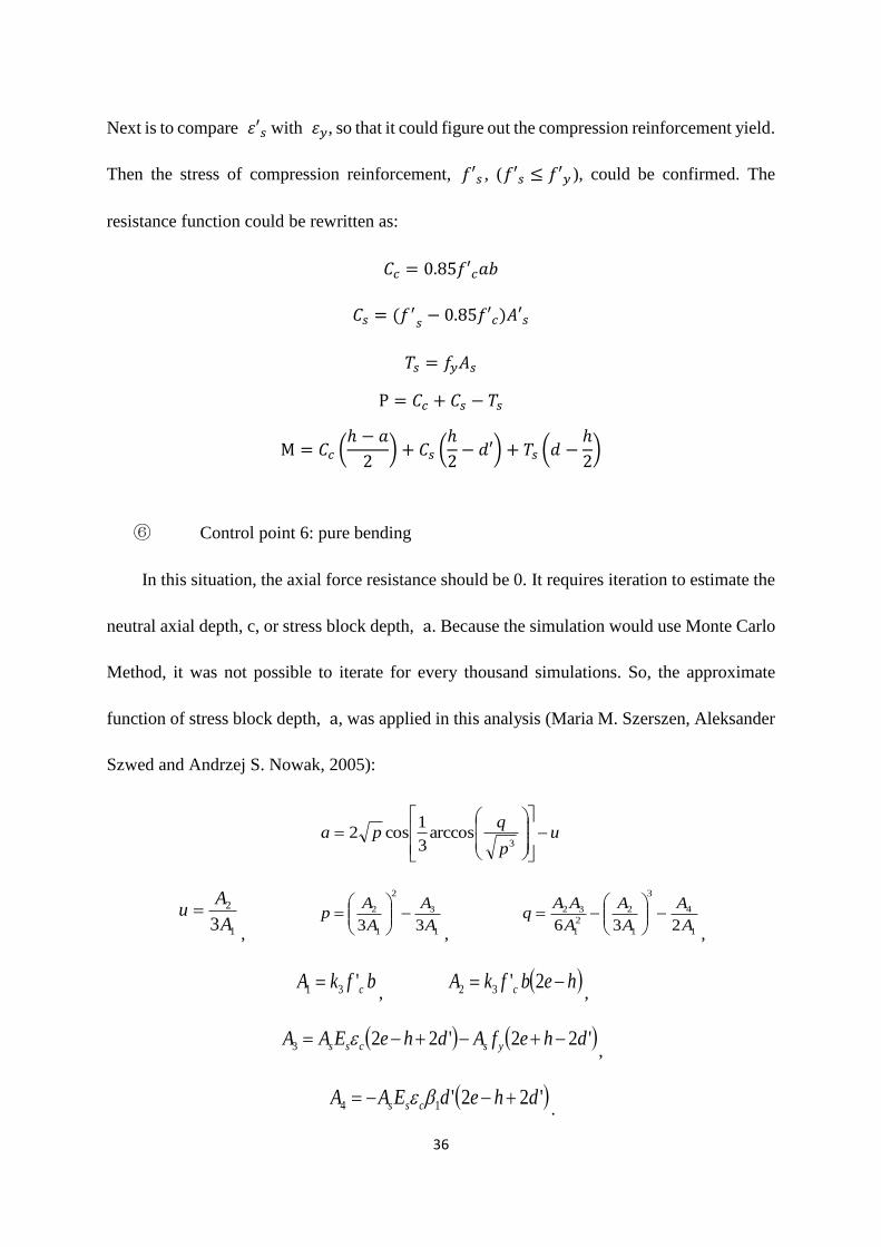
⑥ Control point 6: pure bending

In this situation, the axial force resistance should be 0. It requires iteration to estimate the

neutral axial depth, c, or stress block depth, a. Because the simulation would use Monte Carlo

Method, it was not possible to iterate for every thousand simulations. So, the approximate

function of stress block depth, a, was applied in this analysis (Maria M. Szerszen, Aleksander

Szwed and Andrzej S. Nowak, 2005):

up

qpa −

=

3arccos

3

1cos2

1

2

3A

Au =

, 1

3

2

1

2

33 A

A

A

Ap −

=

, 1

4

3

1

2

2

1

32

236 A

A

A

A

A

AAq −

−=

,

bfkA c'31 = , ( )hebfkA c −= 2'32 ,

( ) ( )'22'223 dhefAdheEAA yscss −+−+−= ,

( )'22'14 dhedEAA css +−−= .

37

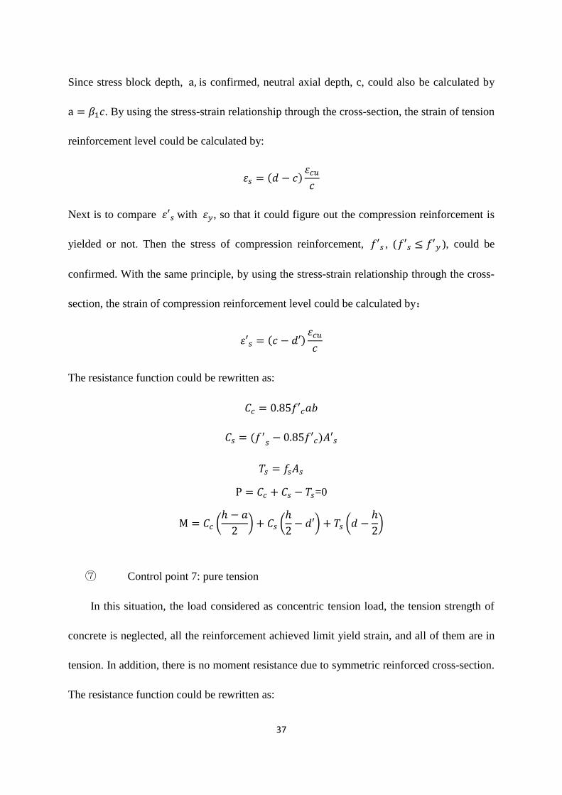
Since stress block depth, a, is confirmed, neutral axial depth, c, could also be calculated by

a = 𝛽1𝑐. By using the stress-strain relationship through the cross-section, the strain of tension

reinforcement level could be calculated by:

𝜀𝑠 = (𝑑 − 𝑐)𝜀𝑐𝑢

𝑐

Next is to compare 𝜀′𝑠 with 𝜀𝑦, so that it could figure out the compression reinforcement is

yielded or not. Then the stress of compression reinforcement, 𝑓′𝑠 , (𝑓′𝑠 ≤ 𝑓′𝑦 ), could be

confirmed. With the same principle, by using the stress-strain relationship through the cross-

section, the strain of compression reinforcement level could be calculated by：


𝑐

The resistance function could be rewritten as:



− 0.85𝑓′𝑐)𝐴′𝑠

𝑇𝑠 = 𝑓𝑠𝐴𝑠

P = 𝐶𝑐 + 𝐶𝑠 − 𝑇𝑠=0

M = 𝐶𝑐 (ℎ − 𝑎

2) + 𝐶𝑠 (

ℎ

2− 𝑑′) + 𝑇𝑠 (𝑑 −

ℎ

2)

⑦ Control point 7: pure tension

In this situation, the load considered as concentric tension load, the tension strength of

concrete is neglected, all the reinforcement achieved limit yield strain, and all of them are in

tension. In addition, there is no moment resistance due to symmetric reinforced cross-section.

The resistance function could be rewritten as:

38

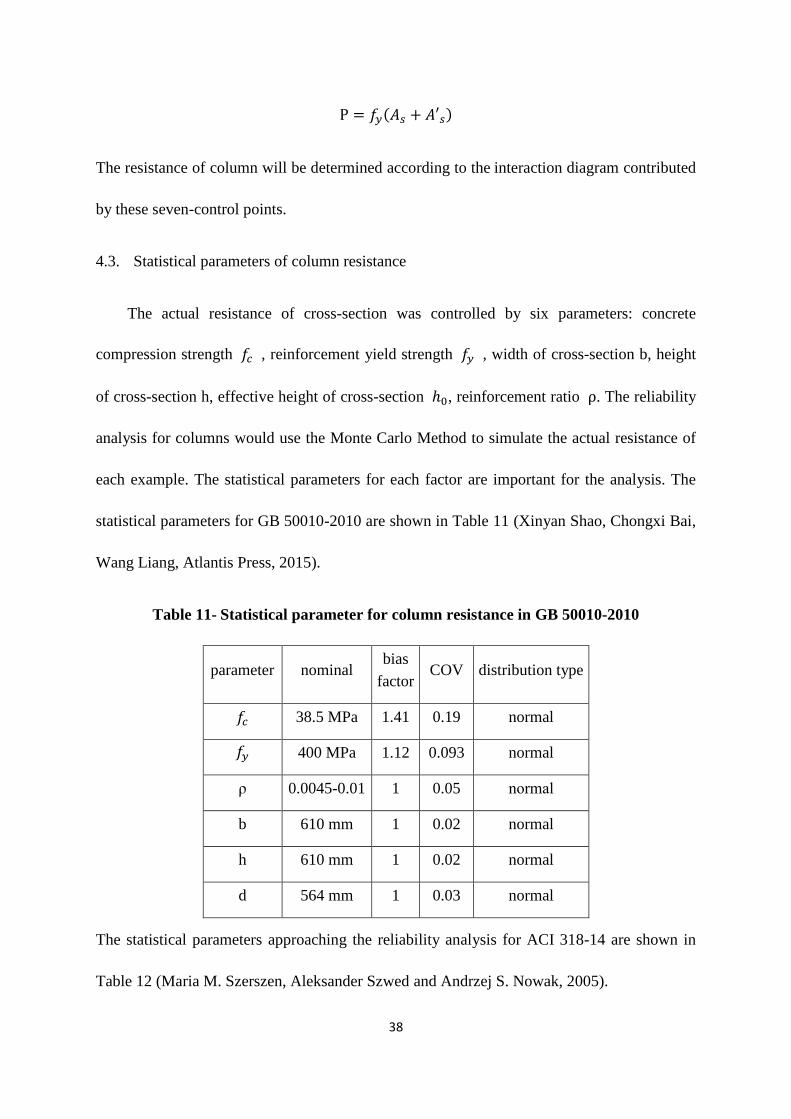
P = 𝑓𝑦(𝐴𝑠 + 𝐴′𝑠)

The resistance of column will be determined according to the interaction diagram contributed

by these seven-control points.

4.3. Statistical parameters of column resistance

The actual resistance of cross-section was controlled by six parameters: concrete

compression strength 𝑓𝑐 , reinforcement yield strength 𝑓𝑦 , width of cross-section b, height

of cross-section h, effective height of cross-section ℎ0, reinforcement ratio ρ. The reliability

analysis for columns would use the Monte Carlo Method to simulate the actual resistance of

each example. The statistical parameters for each factor are important for the analysis. The

statistical parameters for GB 50010-2010 are shown in Table 11 (Xinyan Shao, Chongxi Bai,

Wang Liang, Atlantis Press, 2015).

Table 11- Statistical parameter for column resistance in GB 50010-2010


factor COV distribution type

𝑓𝑐 38.5 MPa 1.41 0.19 normal

𝑓𝑦 400 MPa 1.12 0.093 normal

ρ 0.0045-0.01 1 0.05 normal

b 610 mm 1 0.02 normal

h 610 mm 1 0.02 normal

d 564 mm 1 0.03 normal

The statistical parameters approaching the reliability analysis for ACI 318-14 are shown in

Table 12 (Maria M. Szerszen, Aleksander Szwed and Andrzej S. Nowak, 2005).

39

Table 12- Statistical parameter for column resistance in ACI 318-14


factor COV

distribution

type

𝑓′𝑐 41.4 MPa 1.25 0.1 normal

𝑓𝑦 413.67 MPa 1.145 0.05 normal

ρ 0.0045-0.01 1 0.015 normal

b 610 mm 1.05 0.04 normal

h 610 mm 1.05 0.04 normal

d 564 mm 1.05 0.04 normal

40

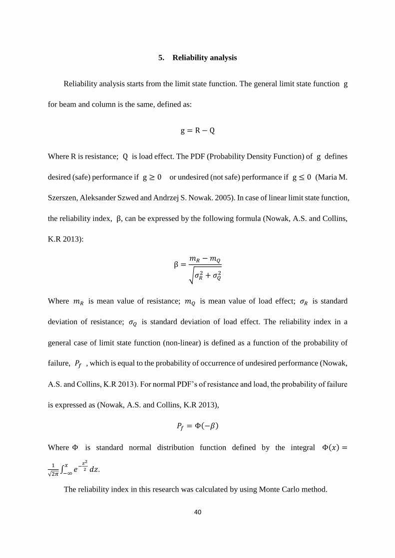
5. Reliability analysis

Reliability analysis starts from the limit state function. The general limit state function g

for beam and column is the same, defined as:

g = R − Q

Where R is resistance; Q is load effect. The PDF (Probability Density Function) of g defines

desired (safe) performance if g ≥ 0 or undesired (not safe) performance if g ≤ 0 (Maria M.

Szerszen, Aleksander Szwed and Andrzej S. Nowak. 2005). In case of linear limit state function,

the reliability index, β, can be expressed by the following formula (Nowak, A.S. and Collins,

K.R 2013):

β =𝑚𝑅 − 𝑚𝑄

√𝜎𝑅2 + 𝜎𝑄

2

Where 𝑚𝑅 is mean value of resistance; 𝑚𝑄 is mean value of load effect; 𝜎𝑅 is standard

deviation of resistance; 𝜎𝑄 is standard deviation of load effect. The reliability index in a

general case of limit state function (non-linear) is defined as a function of the probability of

failure, 𝑃𝑓 , which is equal to the probability of occurrence of undesired performance (Nowak,

A.S. and Collins, K.R 2013). For normal PDF’s of resistance and load, the probability of failure

is expressed as (Nowak, A.S. and Collins, K.R 2013),

𝑃𝑓 = Φ(−𝛽)

Where Φ is standard normal distribution function defined by the integral Φ(𝑥) =

1

√2𝜋∫ 𝑒−

𝑧2

2𝑥

−∞𝑑𝑧.

The reliability index in this research was calculated by using Monte Carlo method.

41

Monte Carlo Procedure:

① Randomly generate values and calculate R .

② Randomly generate values of Q using their probability distribution.

③ Calculate g = R - Q.

④ Save the calculated value of g.

⑤ Repeat steps 1-4 until enough quantity of g values have been generated.

⑥ Plot the results on the probability paper and read the probability of g being negative.

The function of resistance, R, was using resistance functions from two codes, where they

were introduced in chapter three and chapter four. The required nominal (design) resistance,

𝑅𝑛, is:

𝑅𝑛 =𝑄𝑛

𝜙

Where 𝑄𝑛 is the factored load effect. 𝜙 is resistance factor; in ACI 318 𝜙 is equal to 0.9 for

flexure controlled reinforced concrete, 0.65 for compression controlled reinforced concrete for

tied columns. In GB 50009-2012, 𝜙 is only related to the importance of building. For the

examples in this study, it was constantly equal to 1. The mean resistance was determined with

the statistical data stated in chapter three and chapter four. The nominal value of loads was

based on the load combination from ASCE 7 and GB 50009-2012. The mean of load effect

was calculated using the statistical data described in chapter two.

After the reliability index calculated, sensitivity analysis was applied. The sensitivity

analysis is aiming to find out which factor had greater influence on the reliability index of

structures. The analysis was performed taking into account the following parameters for beam

examples: reinforcement ratio (0.2%, 0.3%, 0.4%, 0.5%, 0.6%, 0.7%, 0.8%, 0.9%, 1.0%), load

ratio between live load and dead load plus live load ( 𝐿 𝐷 + 𝐿⁄ =

42

0.1, 0.2, 0.3, 0.4, 0.5, 0.6, 0.7, 0.8, 0.9). For the column examples, the analysis was performed

taking into account the following parameters: concrete strength ( 𝑓′𝑐 =

30 𝑀𝑃𝑎, 40 𝑀𝑃𝑎, 50 𝑀𝑃𝑎, 60𝑀𝑃𝑎), reinforcement ratio ρ (0.5%, 1%, 1.5%, 2%, 3%).

43

6. Comparison of Chines codes and American codes

6.1. Examples of reliability comparison

In this research, there were four pairs of comparison examples, totaling eight examples.

One pair was beams, the other three were columns. Because the column resistance design

method is entirely different in the two series’ codes, it had to have three pairs of examples to

cover all situations.

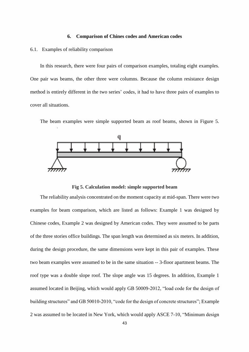
The beam examples were simple supported beam as roof beams, shown in Figure 5.

Fig 5. Calculation model: simple supported beam

The reliability analysis concentrated on the moment capacity at mid-span. There were two

examples for beam comparison, which are listed as follows: Example 1 was designed by

Chinese codes, Example 2 was designed by American codes. They were assumed to be parts

of the three stories office buildings. The span length was determined as six meters. In addition,

during the design procedure, the same dimensions were kept in this pair of examples. These

two beam examples were assumed to be in the same situation -- 3-floor apartment beams. The

roof type was a double slope roof. The slope angle was 15 degrees. In addition, Example 1

assumed located in Beijing, which would apply GB 50009-2012, “load code for the design of

building structures” and GB 50010-2010, “code for the design of concrete structures”; Example

2 was assumed to be located in New York, which would apply ASCE 7-10, “Minimum design

44

loads for buildings and other structures” and ACI 318, “Building Code Requirements for

Reinforced Concrete”. The reinforcement ratio of Example 1 and Example 2 would be

calculated according to the two series’ codes.

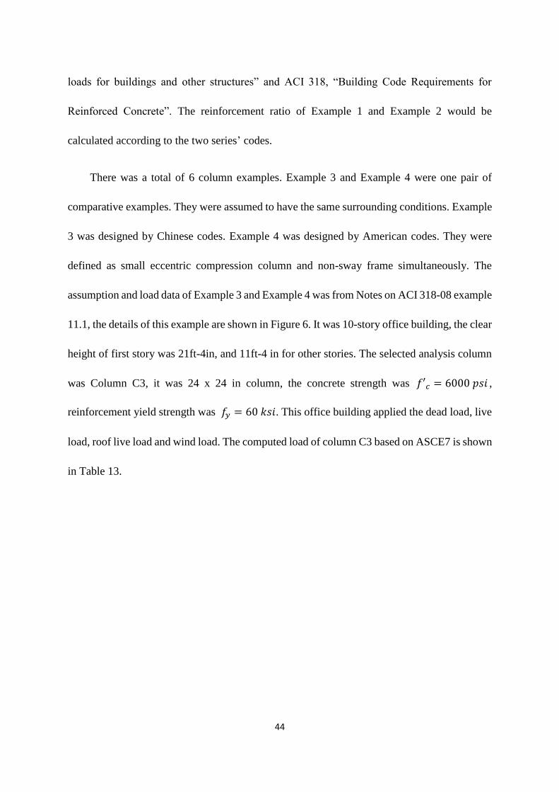
There was a total of 6 column examples. Example 3 and Example 4 were one pair of

comparative examples. They were assumed to have the same surrounding conditions. Example

3 was designed by Chinese codes. Example 4 was designed by American codes. They were

defined as small eccentric compression column and non-sway frame simultaneously. The

assumption and load data of Example 3 and Example 4 was from Notes on ACI 318-08 example

11.1, the details of this example are shown in Figure 6. It was 10-story office building, the clear

height of first story was 21ft-4in, and 11ft-4 in for other stories. The selected analysis column

was Column C3, it was 24 x 24 in column, the concrete strength was 𝑓′𝑐 = 6000 𝑝𝑠𝑖 ,

reinforcement yield strength was 𝑓𝑦 = 60 𝑘𝑠𝑖. This office building applied the dead load, live

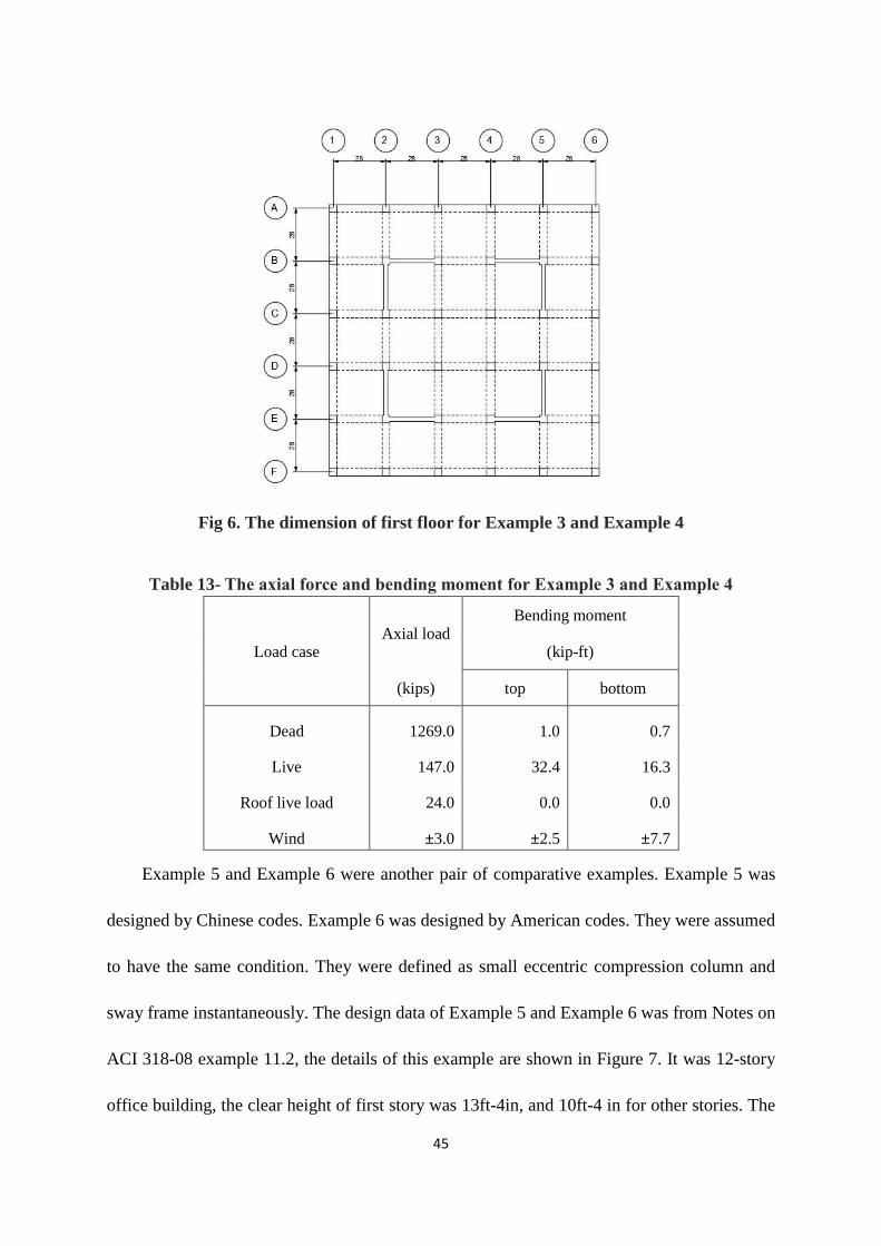
load, roof live load and wind load. The computed load of column C3 based on ASCE7 is shown

in Table 13.

45

Fig 6. The dimension of first floor for Example 3 and Example 4

Table 13- The axial force and bending moment for Example 3 and Example 4

Load case Axial load

Bending moment

(kip-ft)

(kips) top bottom

Dead 1269.0 1.0 0.7

Live 147.0 32.4 16.3

Roof live load 24.0 0.0 0.0

Wind ±3.0 ±2.5 ±7.7

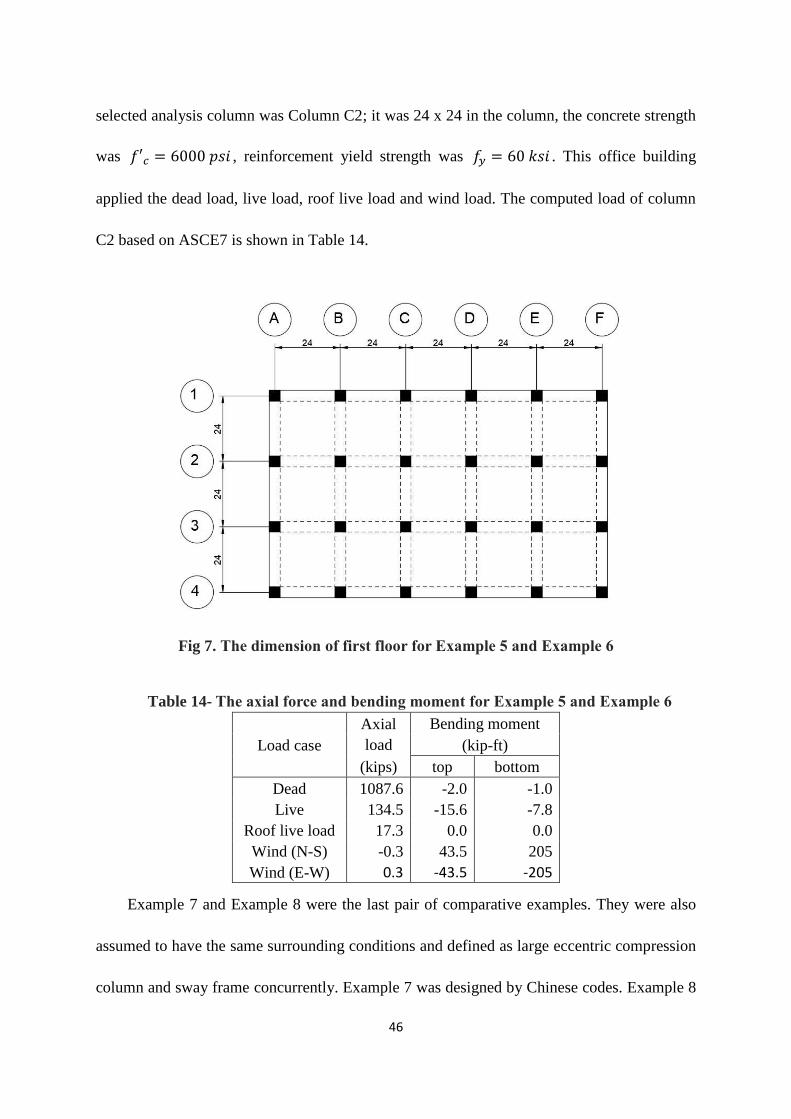
Example 5 and Example 6 were another pair of comparative examples. Example 5 was

designed by Chinese codes. Example 6 was designed by American codes. They were assumed

to have the same condition. They were defined as small eccentric compression column and

sway frame instantaneously. The design data of Example 5 and Example 6 was from Notes on

ACI 318-08 example 11.2, the details of this example are shown in Figure 7. It was 12-story

office building, the clear height of first story was 13ft-4in, and 10ft-4 in for other stories. The

46

selected analysis column was Column C2; it was 24 x 24 in the column, the concrete strength

was 𝑓′𝑐 = 6000 𝑝𝑠𝑖 , reinforcement yield strength was 𝑓𝑦 = 60 𝑘𝑠𝑖 . This office building

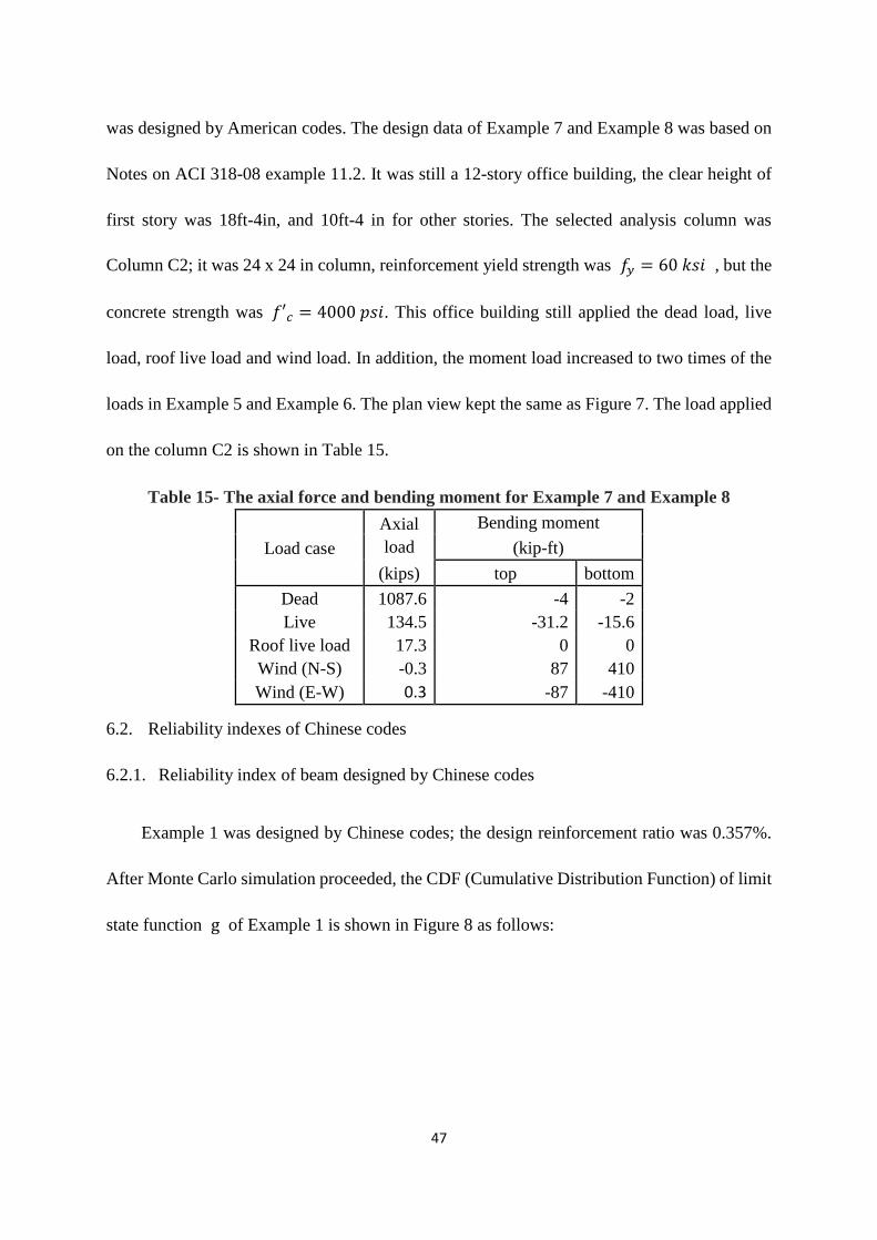
applied the dead load, live load, roof live load and wind load. The computed load of column

C2 based on ASCE7 is shown in Table 14.

Fig 7. The dimension of first floor for Example 5 and Example 6


Load case

Axial

load

Bending moment

(kip-ft)

(kips) top bottom

Dead 1087.6 -2.0 -1.0

Live 134.5 -15.6 -7.8

Roof live load 17.3 0.0 0.0

Wind (N-S) -0.3 43.5 205

Wind (E-W) 0.3 -43.5 -205

Example 7 and Example 8 were the last pair of comparative examples. They were also

assumed to have the same surrounding conditions and defined as large eccentric compression

column and sway frame concurrently. Example 7 was designed by Chinese codes. Example 8

47

was designed by American codes. The design data of Example 7 and Example 8 was based on

Notes on ACI 318-08 example 11.2. It was still a 12-story office building, the clear height of

first story was 18ft-4in, and 10ft-4 in for other stories. The selected analysis column was

Column C2; it was 24 x 24 in column, reinforcement yield strength was 𝑓𝑦 = 60 𝑘𝑠𝑖 , but the

concrete strength was 𝑓′𝑐 = 4000 𝑝𝑠𝑖. This office building still applied the dead load, live

load, roof live load and wind load. In addition, the moment load increased to two times of the

loads in Example 5 and Example 6. The plan view kept the same as Figure 7. The load applied

on the column C2 is shown in Table 15.


Load case

Axial

load

Bending moment

(kip-ft)

(kips) top bottom

Dead 1087.6 -4 -2

Live 134.5 -31.2 -15.6

Roof live load 17.3 0 0

Wind (N-S) -0.3 87 410

Wind (E-W) 0.3 -87 -410

6.2. Reliability indexes of Chinese codes

6.2.1. Reliability index of beam designed by Chinese codes

Example 1 was designed by Chinese codes; the design reinforcement ratio was 0.357%.

After Monte Carlo simulation proceeded, the CDF (Cumulative Distribution Function) of limit

state function g of Example 1 is shown in Figure 8 as follows:

48

Fig 8. The CDF of g of Example 1

The reliability index performed perfectly at a 3.5, which means this design was

economical with enough strength.

6.2.2. Reliability indexes of columns designed by Chinese codes

According to the requirements of GB 50010-2010, the proper reinforcement ratio of

Example 3 was 0.6%, the CDF of limit function is shown in Figure 9.

Fig 9. CDF of g for Example 3

The reliability index was extremely high, because the equilibrium did not determine the

y = 0.0263x - 3.5068

-4

-3

-2

-1

0

1

2

3

4

0 50 100 150 200 250 300

CDF of g

CDF of g (GB) Approximate liner function (GB)

y = 0.0017x - 9.4944

-4

-3

-2

-1

0

1

2

3

4

5

0 1000 2000 3000 4000 5000 6000 7000 8000 9000

CDF of g (GB)

CDF of g (GB) Liner

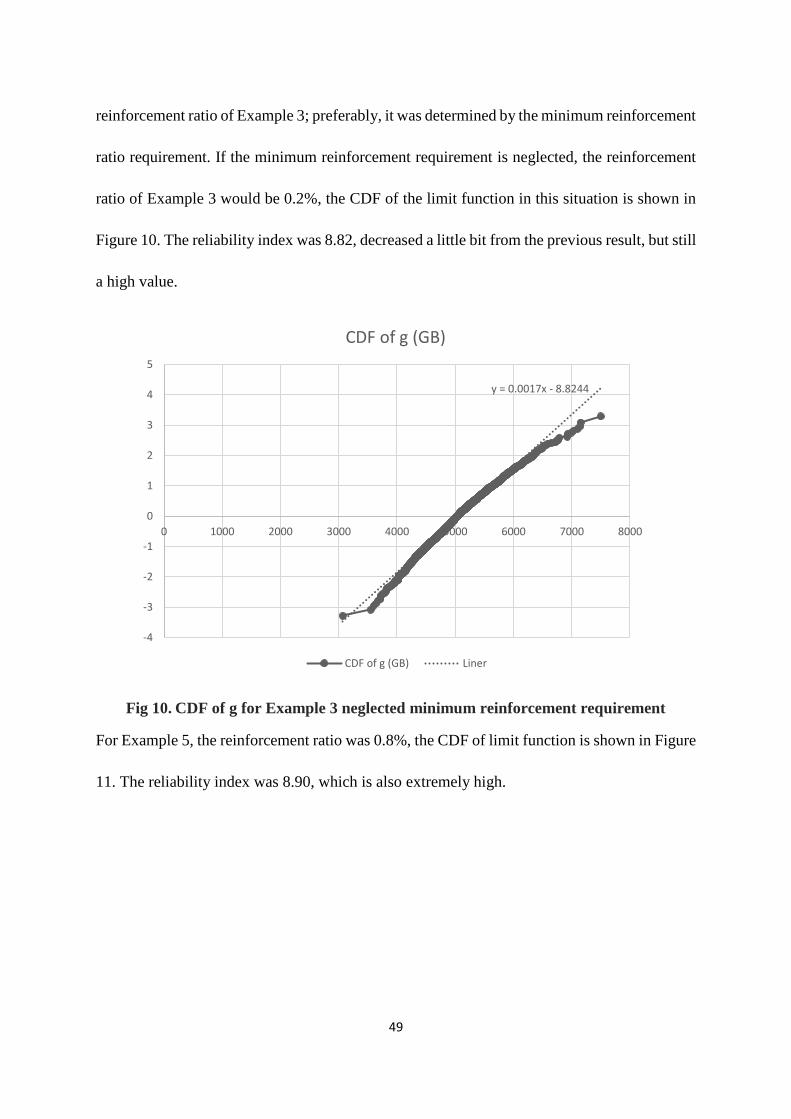
49

reinforcement ratio of Example 3; preferably, it was determined by the minimum reinforcement

ratio requirement. If the minimum reinforcement requirement is neglected, the reinforcement

ratio of Example 3 would be 0.2%, the CDF of the limit function in this situation is shown in

Figure 10. The reliability index was 8.82, decreased a little bit from the previous result, but still

a high value.

Fig 10. CDF of g for Example 3 neglected minimum reinforcement requirement

For Example 5, the reinforcement ratio was 0.8%, the CDF of limit function is shown in Figure

11. The reliability index was 8.90, which is also extremely high.

y = 0.0017x - 8.8244

-4

-3

-2

-1

0

1

2

3

4

5

0 1000 2000 3000 4000 5000 6000 7000 8000

CDF of g (GB)

CDF of g (GB) Liner

50

Fig. 11. CDF of g for Example 5

For Example 7, the reinforcement ratio was 2%, the CDF of limit function is shown in Figure

12. The reliability index was 7.24, which is still extremely high.


6.3. Reliability indexes of American codes

6.3.1. Reliability index of beam designed by American codes

Example 2 was designed according to ACI 318 and ASCE 7. The reinforcement ratio was

0.2713%. The CDF of limit state function g for Example 2 is shown in Figure 13 as follows:

y = 0.0021x - 8.9096

-4

-3

-2

-1

0

1

2

3

4

5

0 1000 2000 3000 4000 5000 6000 7000

CDF of g (GB)

CDF of g (GB) Liner

y = 0.0046x - 7.2395

-5

-4

-3

-2

-1

0

1

2

3

4

0 500 1000 1500 2000 2500 3000

CDF of g (GB)

CDF of g (GB) Liner

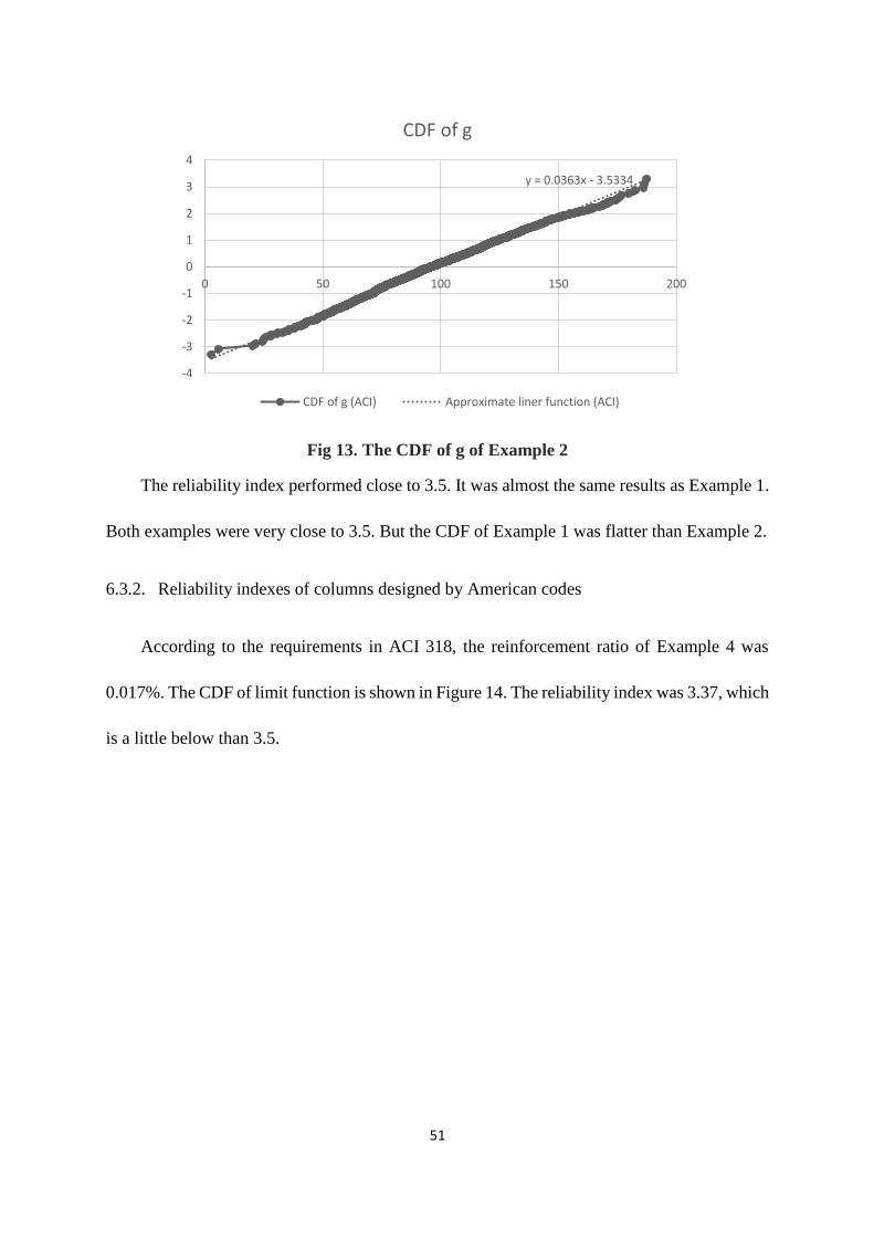
51

Fig 13. The CDF of g of Example 2

The reliability index performed close to 3.5. It was almost the same results as Example 1.

Both examples were very close to 3.5. But the CDF of Example 1 was flatter than Example 2.

6.3.2. Reliability indexes of columns designed by American codes

According to the requirements in ACI 318, the reinforcement ratio of Example 4 was

0.017%. The CDF of limit function is shown in Figure 14. The reliability index was 3.37, which

is a little below than 3.5.

y = 0.0363x - 3.5334

-4

-3

-2

-1

0

1

2

3

4

0 50 100 150 200

CDF of g

CDF of g (ACI) Approximate liner function (ACI)

52


The reinforcement ratio of Example 6 was 0.012%, the CDF of limit function is shown in

Figure 15. The reliability index was 3.79, which achieves the requirement of 3.50.


The reinforcement ratio of Example 8 was 5.7%, the CDF of limit function is shown in

Figure 16. The reliability index was 3.51, which is very close to 3.5.

y = 0.0063x - 3.7935

-6

-5

-4

-3

-2

-1

0

1

2

3

4

-400 -200 0 200 400 600 800 1000 1200

CDF of g (ACI)

CDF of g (ACI) Liner

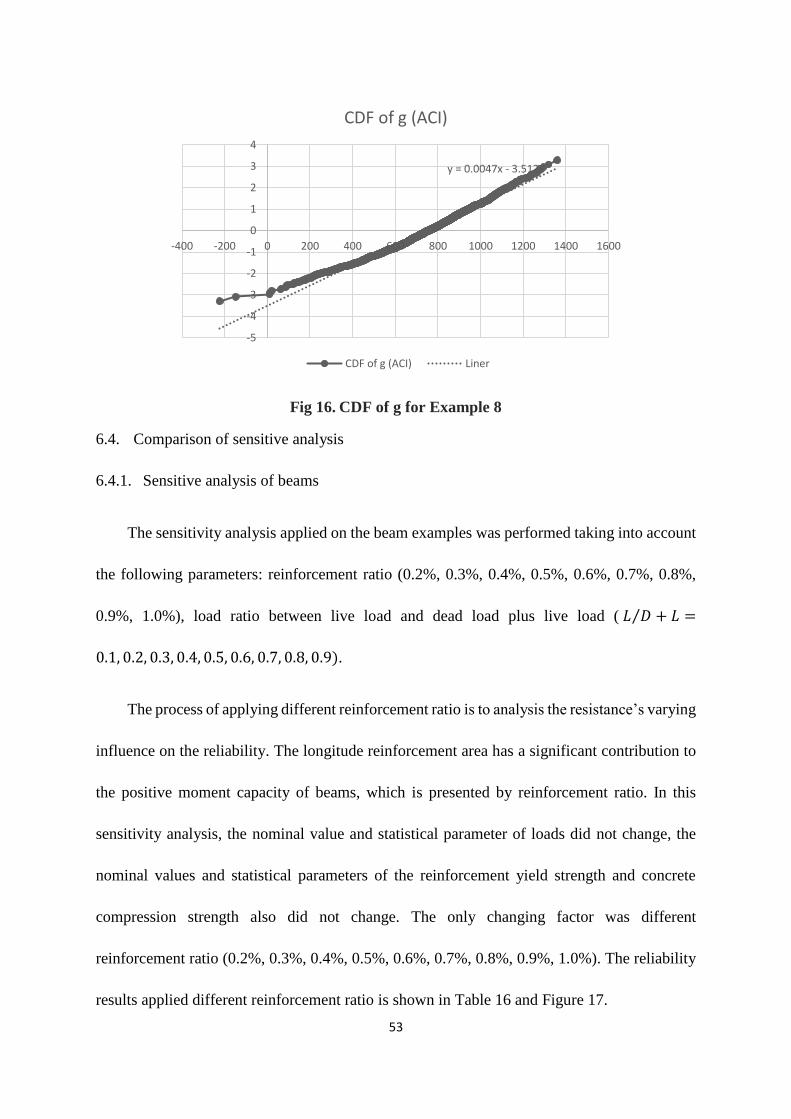
53


6.4. Comparison of sensitive analysis

6.4.1. Sensitive analysis of beams

The sensitivity analysis applied on the beam examples was performed taking into account

the following parameters: reinforcement ratio (0.2%, 0.3%, 0.4%, 0.5%, 0.6%, 0.7%, 0.8%,

0.9%, 1.0%), load ratio between live load and dead load plus live load ( 𝐿 𝐷 + 𝐿⁄ =

0.1, 0.2, 0.3, 0.4, 0.5, 0.6, 0.7, 0.8, 0.9).

The process of applying different reinforcement ratio is to analysis the resistance’s varying

influence on the reliability. The longitude reinforcement area has a significant contribution to

the positive moment capacity of beams, which is presented by reinforcement ratio. In this

sensitivity analysis, the nominal value and statistical parameter of loads did not change, the

nominal values and statistical parameters of the reinforcement yield strength and concrete

compression strength also did not change. The only changing factor was different

reinforcement ratio (0.2%, 0.3%, 0.4%, 0.5%, 0.6%, 0.7%, 0.8%, 0.9%, 1.0%). The reliability

results applied different reinforcement ratio is shown in Table 16 and Figure 17.

y = 0.0047x - 3.5128

-5

-4

-3

-2

-1

0

1

2

3

4

-400 -200 0 200 400 600 800 1000 1200 1400 1600

CDF of g (ACI)

CDF of g (ACI) Liner

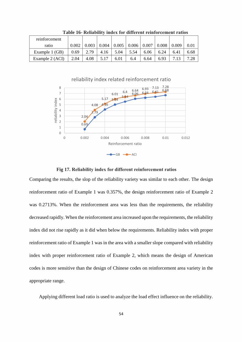
54

Table 16- Reliability index for different reinforcement ratios

reinforcement

ratio 0.002 0.003 0.004 0.005 0.006 0.007 0.008 0.009 0.01

Example 1 (GB) 0.69 2.79 4.16 5.04 5.54 6.06 6.24 6.41 6.68

Example 2 (ACI) 2.04 4.08 5.17 6.01 6.4 6.64 6.93 7.13 7.28

Fig 17. Reliability index for different reinforcement ratios

Comparing the results, the slop of the reliability variety was similar to each other. The design

reinforcement ratio of Example 1 was 0.357%, the design reinforcement ratio of Example 2

was 0.2713%. When the reinforcement area was less than the requirements, the reliability

decreased rapidly. When the reinforcement area increased upon the requirements, the reliability

index did not rise rapidly as it did when below the requirements. Reliability index with proper

reinforcement ratio of Example 1 was in the area with a smaller slope compared with reliability

index with proper reinforcement ratio of Example 2, which means the design of American

codes is more sensitive than the design of Chinese codes on reinforcement area variety in the

appropriate range.

Applying different load ratio is used to analyze the load effect influence on the reliability.

0.69

2.79

4.16

5.045.54

6.06 6.24 6.41 6.68

2.04

4.08

5.17

6.016.4 6.64 6.93 7.13 7.28

0

1

2

3

4

5

6

7

8

0 0.002 0.004 0.006 0.008 0.01 0.012

relia

bili

ty in

dex

Reinforcement ratio

reliability index related reinforcement ratio

GB ACI

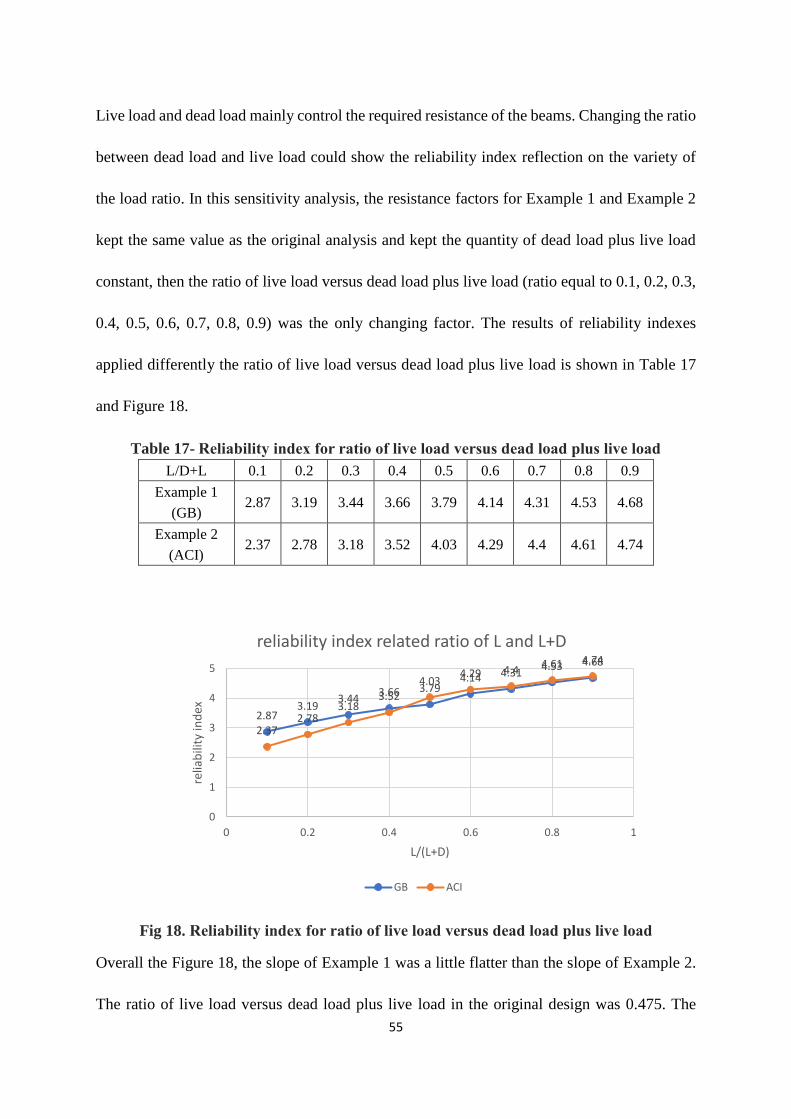
55

Live load and dead load mainly control the required resistance of the beams. Changing the ratio

between dead load and live load could show the reliability index reflection on the variety of

the load ratio. In this sensitivity analysis, the resistance factors for Example 1 and Example 2

kept the same value as the original analysis and kept the quantity of dead load plus live load

constant, then the ratio of live load versus dead load plus live load (ratio equal to 0.1, 0.2, 0.3,

0.4, 0.5, 0.6, 0.7, 0.8, 0.9) was the only changing factor. The results of reliability indexes

applied differently the ratio of live load versus dead load plus live load is shown in Table 17

and Figure 18.

Table 17- Reliability index for ratio of live load versus dead load plus live load

L/D+L 0.1 0.2 0.3 0.4 0.5 0.6 0.7 0.8 0.9

Example 1

(GB) 2.87 3.19 3.44 3.66 3.79 4.14 4.31 4.53 4.68

Example 2

(ACI) 2.37 2.78 3.18 3.52 4.03 4.29 4.4 4.61 4.74

Fig 18. Reliability index for ratio of live load versus dead load plus live load

Overall the Figure 18, the slope of Example 1 was a little flatter than the slope of Example 2.

The ratio of live load versus dead load plus live load in the original design was 0.475. The

2.873.19

3.443.66 3.79

4.14 4.314.53 4.68

2.372.78

3.183.52

4.034.29 4.4

4.61 4.74

0

1

2

3

4

5

0 0.2 0.4 0.6 0.8 1

relia

bili

ty in

dex

L/(L+D)

reliability index related ratio of L and L+D

GB ACI

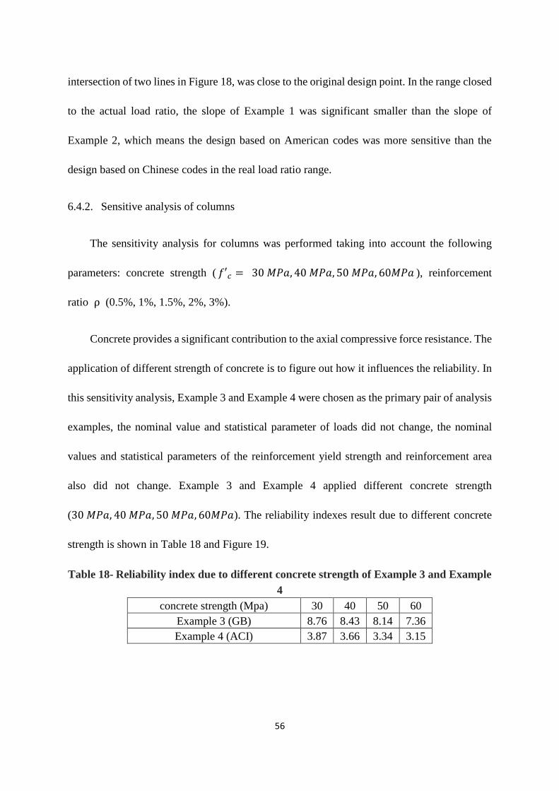
56

intersection of two lines in Figure 18, was close to the original design point. In the range closed

to the actual load ratio, the slope of Example 1 was significant smaller than the slope of

Example 2, which means the design based on American codes was more sensitive than the

design based on Chinese codes in the real load ratio range.

6.4.2. Sensitive analysis of columns

The sensitivity analysis for columns was performed taking into account the following

parameters: concrete strength ( 𝑓′𝑐 = 30 𝑀𝑃𝑎, 40 𝑀𝑃𝑎, 50 𝑀𝑃𝑎, 60𝑀𝑃𝑎 ), reinforcement

ratio ρ (0.5%, 1%, 1.5%, 2%, 3%).

Concrete provides a significant contribution to the axial compressive force resistance. The

application of different strength of concrete is to figure out how it influences the reliability. In

this sensitivity analysis, Example 3 and Example 4 were chosen as the primary pair of analysis

examples, the nominal value and statistical parameter of loads did not change, the nominal

values and statistical parameters of the reinforcement yield strength and reinforcement area

also did not change. Example 3 and Example 4 applied different concrete strength

(30 𝑀𝑃𝑎, 40 𝑀𝑃𝑎, 50 𝑀𝑃𝑎, 60𝑀𝑃𝑎). The reliability indexes result due to different concrete

strength is shown in Table 18 and Figure 19.

Table 18- Reliability index due to different concrete strength of Example 3 and Example

4

concrete strength (Mpa) 30 40 50 60

Example 3 (GB) 8.76 8.43 8.14 7.36

Example 4 (ACI) 3.87 3.66 3.34 3.15

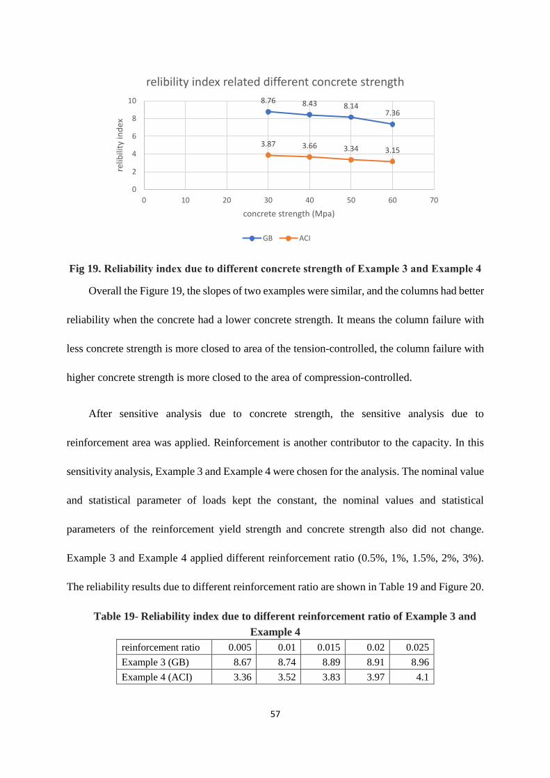
57

Fig 19. Reliability index due to different concrete strength of Example 3 and Example 4

Overall the Figure 19, the slopes of two examples were similar, and the columns had better

reliability when the concrete had a lower concrete strength. It means the column failure with

less concrete strength is more closed to area of the tension-controlled, the column failure with

higher concrete strength is more closed to the area of compression-controlled.

After sensitive analysis due to concrete strength, the sensitive analysis due to

reinforcement area was applied. Reinforcement is another contributor to the capacity. In this

sensitivity analysis, Example 3 and Example 4 were chosen for the analysis. The nominal value

and statistical parameter of loads kept the constant, the nominal values and statistical

parameters of the reinforcement yield strength and concrete strength also did not change.

Example 3 and Example 4 applied different reinforcement ratio (0.5%, 1%, 1.5%, 2%, 3%).

The reliability results due to different reinforcement ratio are shown in Table 19 and Figure 20.

Table 19- Reliability index due to different reinforcement ratio of Example 3 and

Example 4

reinforcement ratio 0.005 0.01 0.015 0.02 0.025

Example 3 (GB) 8.67 8.74 8.89 8.91 8.96

Example 4 (ACI) 3.36 3.52 3.83 3.97 4.1

8.76 8.43 8.147.36

3.87 3.66 3.34 3.15

0

2

4

6

8

10

0 10 20 30 40 50 60 70

relib

ility

ind

ex

concrete strength (Mpa)

relibility index related different concrete strength

GB ACI

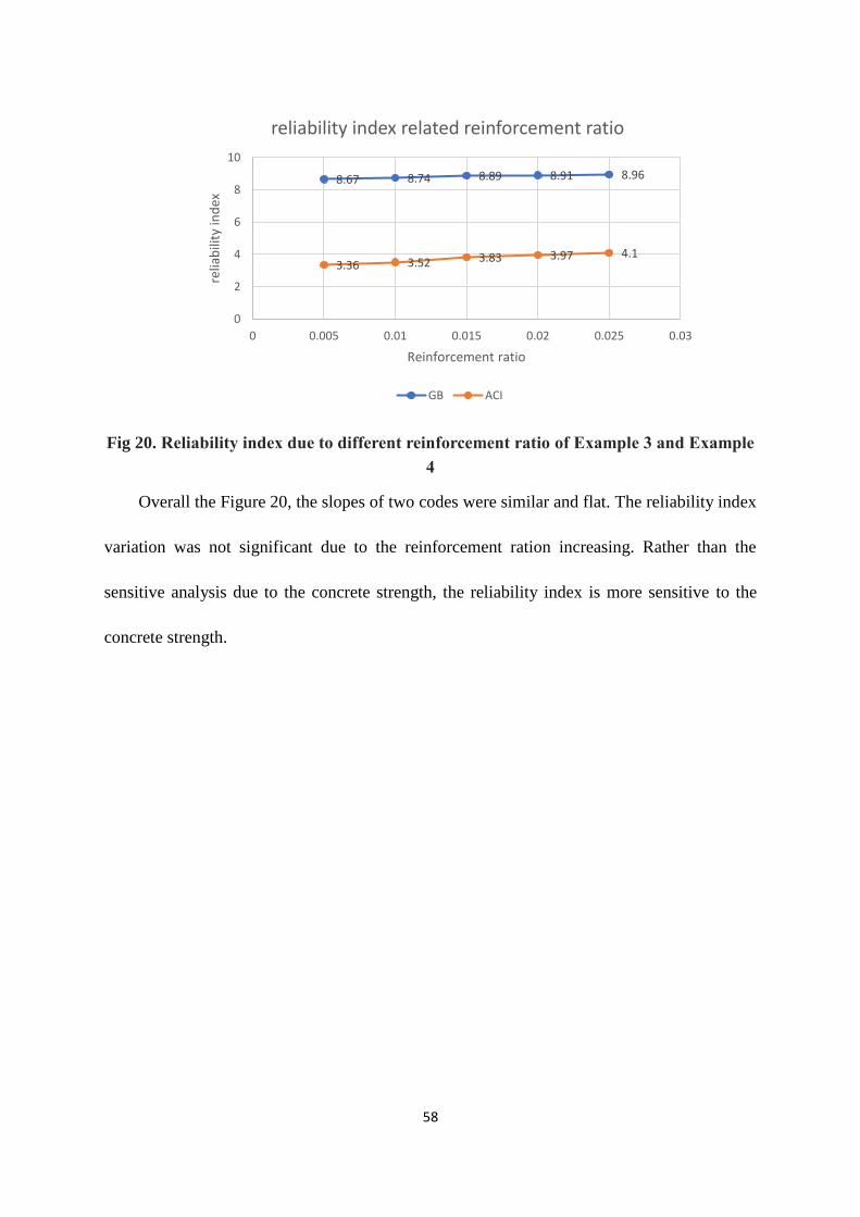
58

Fig 20. Reliability index due to different reinforcement ratio of Example 3 and Example

4

Overall the Figure 20, the slopes of two codes were similar and flat. The reliability index

variation was not significant due to the reinforcement ration increasing. Rather than the

sensitive analysis due to the concrete strength, the reliability index is more sensitive to the

concrete strength.

8.67 8.74 8.89 8.91 8.96

3.36 3.52 3.83 3.97 4.1

0

2

4

6

8

10

0 0.005 0.01 0.015 0.02 0.025 0.03

relia

bili

ty in

dex

Reinforcement ratio

reliability index related reinforcement ratio

GB ACI

59

7. Conclusions

In this dissertation, beams and columns were the main discussed structures for reliability

analysis. For the analysis of beams, the two examples created were designed by different codes.

In addition, the sensitivity analysis was applied to the examples with various reinforcement

areas and different live load ratios. For the analysis of columns, there were six examples, to

ensure coverage the two different design methods in the two different codes (non-sway column

design and sway column design; small eccentric compression design and large eccentric

compression design). Through the analysis procedure, there were some complications were

determined as noted by the following comments:

(1) Both American and Chinese codes could get very excellent performance at the

beams’ reliability with proper reinforcement ratio. But the American codes are

more sensitive to the reliability changing due to load ratio changing.

(2) Chinese code has an entirely different load combination in the design steps. It is

also based on Turkstra’s Rule, but for each variable, the factor number is not same

as ASCE 7-10. Usually the load combination according to Chinese code will get a

little larger value.

(3) The most different part about load is live load, the design live load (nominal value)

is not same. ASCE’s value is larger than GB’s value. In addition, in Chinese code

live load separates into two categories, permanent live load and temporary live

load. These two types of live load have entirely different statistical parameters.

(4) In Chinese code GB 50010-2010, the column design procedure does not consider

about the structures are sway frame or non-sway frame. Instead the Chinese code

60

directly enlarges the eccentricity to gain a larger required moment resistance.

(5) Through the analysis of column models, the reliability index of the columns

designed by Chinese code was extremely high due to ϕ factor. But the resistance

factor ϕ in two series’ codes for resistance is not same. In Chinese code, it

depends on the importance of the building, from 0.9 to 1.1. But in American code,

it is 0.9 for tension-controlled failure, 0.65 for compression-controlled failure.

This difference has a significant influence on the reliability index, especially in the

column reliability analysis.

Overview this research; the Chinese code design method is a little more conservative than

American code on the column design. For the load, even though the load combination is

different, but the results are similar. Only on the live load was there is a significant difference:

it is a more detailed category than in the American code. As for the resistance factor ϕ, it

should have more research on it for Chinese code.

61

References

ACI318. Building Code Requirements for Reinforced Concrete. Detroit: American Concrete

Institute Standard Committee 318, 2014.

ASCE7-10. Minimum design loads for buildings and other structures. Reston: American

society of civil engineers, 2010.

Bartlett, F.M., H.P. Hong, and W. Zhou. "Load factor calibration for the proposed 2005 edition

of the National Building Code of Canada: Statistics of loads and load effects." Can. J.

Civ. Eng., 2003: 30(2): 429-439.

Bazovsky, Igor. Reliability Theory and Practice. New York: Dover Publications. INC, 1961.

Ellingwood, Bruce R., and Paulos Beraki Tekie. "Wind load statistics for probability-based

structural design." J. Struct. Eng, 1999: 125(4): 453-463.

GB50009-2012. Load Code for Deign of Building Structures. Beijing: Ministry of Housing and

Urban-Rural Development of the People's Republic of China, 2012.

GB50010-2010. Code for Design Concrete Structures. Beijing: Ministry of Housing and

Urban-Rural Development of the People's Republic of China, 2010.

GB50153-2008. Unified Standard for Reliability Design of Engineering Structure. Beijing:

Ministry of Housing and Urban-Rural Development of the People's Republic of China,

2008.

Hou, Bonian, and Caiang Wei. "Statistical Analysis of Snow Loads in the Unified Standard for

Building Structure Design." Industrial Construction, 1982: 12 (2): 61-64.

Lee, Kyung Ho, and David V. Rosowsky. "Site-Specific Snow Load Models and Hazard Curves

for Probabilistic Design." Nat. Hazards Rev, 2005: 6(3): 109-120.

Li, Zhenchang, and Jiayan Wang. "Statistical Analysis of Dead Loads in the Unified Standard

for Building Structure Design." Industrial Building, 1982: 12 (3) :55-58.

Nowak, A.S., and K.R. Collins. Reliability of Structures. New York: CRC Press, 2013.

Nowak, Andrzej S., and Maria M. Szerszen. "Calibration of Design Code for Buildings (ACI

318) Part 1: Statistical Models for Resistance." Structural Journal (University of

Michigan), 2003: 377-382.

Shao, Xinyan, Chongxi Bai, and Wang Liang. "Statistical Resistance and Reliability Analysis

of Steel-Concrete Composite Beams." Proceedings of the International Conference on

Advances in Energy, Environment and Chemical Engineering. Changsha, China:

Atlantis Press, 2015. 545-549.

Szerszen, Maria M., Aleksander Szwed, and Andrzej S. Nowak. "RELIABILITY ANALYSIS

FOR ECCENTRICALLY LOADED COLUMNS." ACI Structural Journal, 2005: 676-

62

688.

Tu, Xiangyuan. "Statistical Analysis of Wind Loads in the Unified Standard for Building

Structure Design." Industrial Buildings, 1982: 12 (2): 57-60.

Comparison of the reliability index between American codes ...

Documents

Transcript of Comparison of the reliability index between American codes ...