Comparison of Routing Metrics

8/4/2019 Comparison of Routing Metrics

http://slidepdf.com/reader/full/comparison-of-routing-metrics 1/12

Comparison of Routing Metrics for Static Multi-HopWireless Networks

Richard Draves Jitendra Padhye Brian Zill

Microsoft Research

{richdr, padhye, bzill}@microsoft.com

ABSTRACT

Routing protocols for wireless ad hoc networks have tradi-tionally focused on finding paths with minimum hop count.However, such paths can include slow or lossy links, leadingto poor throughput. A routing algorithm can select betterpaths by explicitly taking the quality of the wireless linksinto account. In this paper, we conduct a detailed, empirical

evaluation of the performance of three link-quality metrics—ETX, per-hop RTT, and per-hop packet pair—and comparethem against minimum hop count. We study these metricsusing a DSR-based routing protocol running in a wirelesstestbed. We find that the ETX metric has the best per-formance when all nodes are stationary. We also find thatthe per-hop RTT and per-hop packet-pair metrics performpoorly due to self-interference. Interestingly, the hop-countmetric outperforms all of the link-quality metrics in a sce-nario where the sender is mobile.

Categories and Subject Descriptors

C.2.1 [Network Architecture and Design]: WirelessNetworks

General TermsMeasurement, Performance, Experimentation

Keywords

Wireless multi-hop networks, Routing

1. INTRODUCTIONRouting in ad hoc wireless networks has been an active

area of research for many years. Much of the original workin the area was motivated by mobile application environ-ments, such as battlefield ad hoc networks. The primary fo-cus in such environments is to provide scalable routing in thepresence of mobile nodes. Recently, interesting commercialapplications of multi-hop wireless networks have emerged.One example of such applications is “community wireless

Permission to make digital or hard copies of all or part of this work forpersonal or classroom use is granted without fee provided that copies arenot made or distributed for profit or commercial advantage and that copiesbear this notice and the full citation on the first page. To copy otherwise, torepublish, to post on servers or to redistribute to lists, requires prior specificpermission and/or a fee.SIGCOMM’04, Aug. 30–Sept. 3, 2004, Portland, Oregon, USA.Copyright 2004 ACM 1-58113-862-8/04/0008 ...$5.00.

networks” [27, 26, 16, 6]. In such networks, most of thenodes are either stationary or minimally mobile. The focusof routing algorithms in such networks is on improving thenetwork capacity or the performance of individual transfers.

Most current ad hoc routing protocols select paths thatminimize hop count [15, 24, 23, 22]. In static ad hoc wirelessnetworks, minimal hop count paths can have poor perfor-mance because they tend to include wireless links between

distant nodes. These long wireless links can be slow or lossy,leading to poor throughput [9]. A routing algorithm can se-lect better paths by explicitly taking into account the qualityof wireless links.

Researchers have proposed many metrics to measure wire-less link quality, but to our knowledge, the relative perfor-mance of these metrics for the purpose of routing in staticad hoc wireless networks has not been investigated. In thispaper, we study the performance of three link-quality met-rics, and compare them against minimum hop-count routing.The first metric is called “Expected Transmission Count”(ETX). This metric is based on measuring the loss rate of broadcast packets between pairs of neighboring nodes [9].The second metric is called “Per-hop Round Trip Time”

(RTT). This metric is based on measuring the round tripdelay seen by unicast probes between neighboring nodes [1].The third metric is called “Per-hop Packet Pair Delay” (Pk-tPair). This metric is based on measuring the delay be-tween a pair of back-to-back probes to a neighboring node.We incorporated these metrics in an ad hoc routing proto-col based on DSR. We deployed this protocol on a 23-nodewireless testbed, and experimented with various traffic sce-narios such as long-lived TCP flows, multiple simultaneousdata transfers and simulated web traffic. We also considereda scenario involving some mobility.

The main contributions of the paper are the following: (i)We describe a routing protocol that incorporates the notionof link quality metrics. (ii) We present detailed experimentalresults to show that in scenarios with stationary nodes, the

ETX metric out-performs hop-count although it uses longerpaths. This is in contrast with the results in [9], in whichthe authors saw little or no gain from ETX in a DSR-basedrouting protocol. (iii) We show that the one-hop RTT andone-hop packet-pair metrics perform poorly, because theirload-sensitivity leads to self-interference. (iv) We show thatin a scenario involving a mobile sender, minimum hop-countrouting performs considerably better than link-quality rout-ing because the metrics do not react sufficiently quickly.



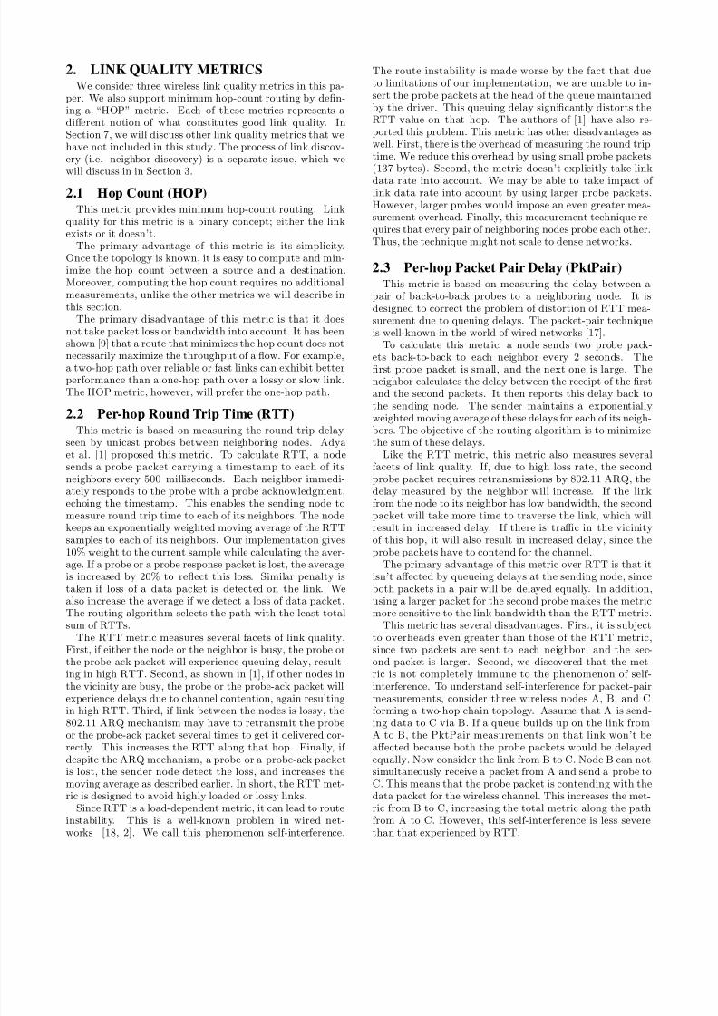
2. LINK QUALITY METRICSWe consider three wireless link quality metrics in this pa-

per. We also support minimum hop-count routing by defin-ing a “HOP” metric. Each of these metrics represents adifferent notion of what constitutes good link quality. InSection 7, we will discuss other link quality metrics that wehave not included in this study. The process of link discov-ery (i.e. neighbor discovery) is a separate issue, which wewill discuss in in Section 3.

2.1 Hop Count (HOP)This metric provides minimum hop-count routing. Link

quality for this metric is a binary concept; either the linkexists or it doesn’t.

The primary advantage of this metric is its simplicity.Once the topology is known, it is easy to compute and min-imize the hop count between a source and a destination.Moreover, computing the hop count requires no additionalmeasurements, unlike the other metrics we will describe inthis section.

The primary disadvantage of this metric is that it doesnot take packet loss or bandwidth into account. It has beenshown [9] that a route that minimizes the hop count does not

necessarily maximize the throughput of a flow. For example,a two-hop path over reliable or fast links can exhibit betterperformance than a one-hop path over a lossy or slow link.The HOP metric, however, will prefer the one-hop path.

2.2 Per-hop Round Trip Time (RTT)This metric is based on measuring the round trip delay

seen by unicast probes between neighboring nodes. Adyaet al. [1] proposed this metric. To calculate RTT, a nodesends a probe packet carrying a timestamp to each of itsneighbors every 500 milliseconds. Each neighbor immedi-ately responds to the probe with a probe acknowledgment,echoing the timestamp. This enables the sending node tomeasure round trip time to each of its neighbors. The nodekeeps an exponentially weighted moving average of the RTTsamples to each of its neighbors. Our implementation gives10% weight to the current sample while calculating the aver-age. If a probe or a probe response packet is lost, the averageis increased by 20% to reflect this loss. Similar penalty istaken if loss of a data packet is detected on the link. Wealso increase the average if we detect a loss of data packet.The routing algorithm selects the path with the least totalsum of RTTs.

The RTT metric measures several facets of link quality.First, if either the node or the neighbor is busy, the probe orthe probe-ack packet will experience queuing delay, result-ing in high RTT. Second, as shown in [1], if other nodes inthe vicinity are busy, the probe or the probe-ack packet willexperience delays due to channel contention, again resulting

in high RTT. Third, if link between the nodes is lossy, the802.11 ARQ mechanism may have to retransmit the probeor the probe-ack packet several times to get it delivered cor-rectly. This increases the RTT along that hop. Finally, if despite the ARQ mechanism, a probe or a probe-ack packetis lost, the sender node detect the loss, and increases themoving average as described earlier. In short, the RTT met-ric is designed to avoid highly loaded or lossy links.

Since RTT is a load-dependent metric, it can lead to routeinstability. This is a well-known problem in wired net-works [18, 2]. We call this phenomenon self-interference.

The route instability is made worse by the fact that dueto limitations of our implementation, we are unable to in-sert the probe packets at the head of the queue maintainedby the driver. This queuing delay significantly distorts theRTT value on that hop. The authors of [1] have also re-ported this problem. This metric has other disadvantages aswell. First, there is the overhead of measuring the round triptime. We reduce this overhead by using small probe packets(137 bytes). Second, the metric doesn’t explicitly take link

data rate into account. We may be able to take impact of link data rate into account by using larger probe packets.However, larger probes would impose an even greater mea-surement overhead. Finally, this measurement technique re-quires that every pair of neighboring nodes probe each other.Thus, the technique might not scale to dense networks.

2.3 Per-hop Packet Pair Delay (PktPair)This metric is based on measuring the delay between a

pair of back-to-back probes to a neighboring node. It isdesigned to correct the problem of distortion of RTT mea-surement due to queuing delays. The packet-pair techniqueis well-known in the world of wired networks [17].

To calculate this metric, a node sends two probe pack-

ets back-to-back to each neighbor every 2 seconds. Thefirst probe packet is small, and the next one is large. Theneighbor calculates the delay between the receipt of the firstand the second packets. It then reports this delay back tothe sending node. The sender maintains a exponentiallyweighted moving average of these delays for each of its neigh-bors. The objective of the routing algorithm is to minimizethe sum of these delays.

Like the RTT metric, this metric also measures severalfacets of link quality. If, due to high loss rate, the secondprobe packet requires retransmissions by 802.11 ARQ, thedelay measured by the neighbor will increase. If the linkfrom the node to its neighbor has low bandwidth, the secondpacket will take more time to traverse the link, which willresult in increased delay. If there is traffic in the vicinityof this hop, it will also result in increased delay, since theprobe packets have to contend for the channel.

The primary advantage of this metric over RTT is that itisn’t affected by queueing delays at the sending node, sinceboth packets in a pair will be delayed equally. In addition,using a larger packet for the second probe makes the metricmore sensitive to the link bandwidth than the RTT metric.

This metric has several disadvantages. First, it is subjectto overheads even greater than those of the RTT metric,since two packets are sent to each neighbor, and the sec-ond packet is larger. Second, we discovered that the met-ric is not completely immune to the phenomenon of self-interference. To understand self-interference for packet-pairmeasurements, consider three wireless nodes A, B, and C

forming a two-hop chain topology. Assume that A is send-ing data to C via B. If a queue builds up on the link fromA to B, the PktPair measurements on that link won’t beaffected because both the probe packets would be delayedequally. Now consider the link from B to C. Node B can notsimultaneously receive a packet from A and send a probe toC. This means that the probe packet is contending with thedata packet for the wireless channel. This increases the met-ric from B to C, increasing the total metric along the pathfrom A to C. However, this self-interference is less severethan that experienced by RTT.



Ethernet 802.11 802.16, etc.

Mesh Connectivity Layer (with LQSR)

IPv4 IPv6 IPX, etc.

Figure 1: Our architecture multiplexes multiplephysical links into a single virtual link.

2.4 Expected Transmission Count (ETX)This metric estimates the number of retransmissions neededto send unicast packets by measuring the loss rate of broad-cast packets between pairs of neighboring nodes. De Coutoet al. [9] proposed ETX. To compute ETX, each node broad-casts a probe packet every second. The probe contains thecount of probes received from each neighboring node in theprevious 10 seconds. Based on these probes, a node cancalculate the loss rate of probes on the links to and fromits neighbors. Since the 802.11 MAC does not retransmitbroadcast packets, these counts allow the sender to esti-mate the number of times the 802.11 ARQ mechanism willretransmit a unicast packet.

To illustrate this, consider two nodes A and B. Assumethat node A has received 8 probe packets from B in the pre-

vious 10 seconds, and in the last probe packet, B reportedthat it had received 9 probe packets from A in the previous10 seconds. Thus, the loss rate of packets from A to B is0.1, while the loss rate of packets from B to A is 0.2. Asuccessful unicast data transfer in 802.11 involves sendingthe data packet and receiving a link-layer acknowledgmentfrom the receiver. Thus, the probability that the data packetwill be successfully transmitted from A to B in a single at-tempt is (1 − 0.1) × (1 − 0.2) = 0.72. If either the data orthe ack is lost, the 802.11 ARQ mechanism will retransmitthe packet. If we assume that losses are independent, theexpected number of retransmissions before the packet is suc-cessfully delivered is 1/0.72 = 1.39. This is the value of theETX metric for the link from A to B. The routing protocol

finds a path that minimizes the sum of the expected numberof retransmissions.Node A calculates a new ETX value for the link from A to

B every time it receives a probe from B. In our implementa-tion of the ETX metric, the node maintains an exponentiallyweighted moving average of ETX samples. There is no ques-tion of taking 20% p enalty for lost probe packets. Penaltyis taken only upon loss of a data packet.

ETX has several advantages. Since each node broadcaststhe probe packets instead of unicasting them, the probingoverhead is substantially reduced. The metric suffers littlefrom self-interference since we are not measuring delays.

The main disadvantage of this metric is that since broad-cast probe packets are small, and are sent at the lowestpossible data rate (6Mbps in case of 802.11a), they may not

experience the same loss rate as data packets sent at higherrates. Moreover, the metric does not directly account forlink load or data rate. A heavily loaded link may have verylow loss rate, and two links with different data rates mayhave the same loss rate.

3. AD HOC ROUTING ARCHITECTUREWe implement ad hoc routing and link-quality measure-

ment in a module that we call the Mesh Connectivity Layer(MCL). Architecturally, MCL is a loadable Windows driver.

It implements a virtual network adapter, so that to the restof the system the ad hoc network appears as an additional(virtual) network link. MCL routes using a modified ver-sion of DSR [15] that we call Link-Quality Source Routing(LQSR). We have modified DSR extensively to improve itsbehavior, most significantly to support link-quality metrics.In this section, we briefly review our architecture and im-plementation to provide background for understanding theperformance results. More architectural and implementa-

tion details are available in [10].The MCL driver implements an interposition layer be-

tween layer 2 (the link layer) and layer 3 (the network layer).To higher-layer software, MCL appears to be just anotherethernet link, albeit a virtual link. To lower-layer software,MCL appears to be just another protocol running over thephysical link. See Figure 1 for a diagram.

This design has two significant advantages. First, higher-layer software runs unmodified over the ad hoc network. Inour testbed, we run both IPv4 and IPv6 over the ad hocnetwork. No modifications to either network stack were re-quired. Second, the ad hoc routing runs over heterogeneouslink layers. Our current implementation supports ethernet-like physical link layers (eg 802.11 and 802.3). The virtual

MCL network adapter can multiplex several physical net-work adapters, so the ad hoc network can extend acrossheterogeneous physical links.

In the simple configuration shown in Figure 1, the MCLdriver binds to all the physical adapters and IP binds onlyto the MCL virtual adapter. This avoids multi-homing atthe IP layer. However other configurations are also possible.In our testbed deployment, the nodes have both an 802.11adapter for the ad hoc network and an ethernet adapterfor management and diagnosis. We configure MCL to bindonly to the 802.11 adapter. The IP stack binds to bothMCL and the ethernet adapter. Hence the mesh nodes aremulti-homed at the IP layer, so they have both a mesh IPaddress and a management IP address. We prevent MCLfrom binding to the management ethernet adapter, so the ad

hoc routing does not discover the ethernet as a high-qualitysingle-hop link between all mesh nodes.

The MCL adapter has its own 48-bit virtual ethernet ad-dress, distinct from the layer-2 addresses of the underlyingphysical adapters. The mesh network functions just like anethernet, except that it has a smaller MTU. To allow roomfor the LQSR headers, it exposes a 1280-byte MTU insteadof the normal 1500-byte ethernet MTU. Our 802.11 driversdo not support the maximum 2346-byte 802.11 frame size.

The MCL driver implements a version of DSR that we callLink-Quality Source Routing (LQSR). LQSR implementsall the basic DSR functionality, including Route Discov-ery (Route Request and Route Reply messages) and RouteMaintenance (Route Error messages). LQSR uses a linkcache instead of a route cache, so fundamentally it is a link-state routing protocol like OSPF [20]. The primary changesin LQSR versus DSR relate to its implementation at layer2.5 instead of layer 3 and its support for link-quality metrics.

Due to the layer 2.5 architecture, LQSR uses 48-bit vir-tual ethernet addresses. All LQSR headers, including SourceRoute, Route Request, Route Reply, and Route Error, use48-bit virtual addresses instead of 32-bit IP addresses.

We have modified DSR in several ways to support routingaccording to link-quality metrics. These include modifica-tions to Route Discovery and Route Maintenance plus new



mechanisms for Metric Maintenance. Our design does notassume that the link-quality metric is symmetric.

First, LQSR Route Discovery supports link metrics. Whena node receives a Route Request and appends its own ad-dress to the route in the Route Request, it also appends themetric for the link over which the packet arrived. When anode sends a Route Reply, the reply carries back the com-plete list of link metrics for the route.

Once Route Discovery populates a node’s link cache, the

cached link metrics must be kept reasonably up-to-date forthe node’s routing to remain accurate. In Section 5.2 weshow that link metrics do vary considerably, even whennodes are not mobile. LQSR tackles this with two separateMetric Maintenance mechanisms.

LQSR uses a reactive mechanism to maintain the metricsfor the links which it is actively using. When a node sendsa source-routed packet, each intermediate node updates thesource route with the current metric for the next (outgoing)link. This carries up-to-date link metrics forward with thedata. To get the link metrics back to the source of the packetflow (where they are needed for the routing computation),we have the recipient of a source-routed data packet senda gratuitous Route Reply back to the source, conveying the

up-to-date link metrics from the arriving Source Route. Thisgratuitous Route Reply is delayed up to one second waitingfor a piggy-backing opportunity.

LQSR uses a proactive background mechanism to main-tain the metrics for all links. Occasionally each LQSR nodesend a Link Info message. The Link Info carries current met-rics for each link from the originating node. The Link Infois piggy-backed on a Route Request, so it floods throughoutthe neighborhood of the node. LQSR piggy-backs Link Infomessages on all Route Requests when possible.

The link metric support also affects Route Maintenance.When Route Maintenance notices that a link is not func-tional (because a requested Ack has not been received), itpenalizes the link’s metric and sends a Route Error. TheRoute Error carries the link’s updated metric back to the

source of the packet.Our LQSR implementation includes the usual DSR con-

ceptual data structures. These include a Send Buffer, forbuffering packets while performing Route Discovery; a Main-tenance Buffer, for buffering packets while performing RouteMaintenance; and a Route Request table, for suppressingduplicate Route Requests. The LQSR implementation of Route Discovery omits some optimizations that are not worth-while in our environment. In practice, Route Discovery isalmost never required in our testbed so we have not opti-mized it. In particular, LQSR nodes do not reply to RouteRequests from their link cache. Only the target of a RouteRequest sends a Route Reply. Furthermore, nodes do notsend Route Requests with a hop limit to restrict their prop-agation. Route Requests always flood throughout the adhoc network. Nodes do cache information from overheardRoute Requests.

The Windows 802.11 drivers do not support promiscuousmode and they do not indicate whether a packet was suc-cessfully transmitted. Hence our implementation of RouteMaintenance uses explicit acknowledgments instead of pas-sive acknowledgments or link-layer acknowledgments. Everysource-routed packet carries an Ack Request option. A nodeexpects an Ack from the next hop within 500ms. The Ackoptions are delayed briefly (up to 80ms) so that they may be

piggy-backed on other packets flowing in the reverse direc-tion. Also later Acks squash (replace) earlier Acks that arewaiting for transmission. As a result of these techniques, theacknowledgment mechanism does not add significant byte orpacket overhead.

The LQSR implementation of Route Maintenance alsoomits some optimizations. We do not implement “Auto-matic Route Shortening,” because of the lack of promiscu-ous mode. We also do not implement “Increased Spreading

of Route Error Messages”. This is not important becauseLQSR will not reply to a Route Request from (possibly stale)cached data. When LQSR Route Maintenance detects a bro-ken link, it does not remove from the transmit queue otherpackets waiting to be sent over the broken link, since Win-dows drivers do not provide access to the transmit queue.However, LQSR nodes do learn from Route Error messagesthat they forward.

LQSR supports a form of DSR’s “Packet Salvaging” orretransmission. Salvaging allows a node to try a differentroute when it is forwarding a source-routed packet and dis-covers that the next hop is not reachable. The acknowledg-ment mechanism does not allow every packet to be salvagedbecause it is primarily designed to detect when links fail.

When sending a packet over a link, if the link has recently(within 250ms) been confirmed to be functional, we requestan Ack as usual but we do not buffer the packet for possiblesalvaging. This design allows for salvaging the first packetsin a new connection and salvaging infrequent connection-lesscommunication, but relies on transport-layer retransmissionfor active connections. In our experience, packets traversing“cold” routes are more vulnerable to loss from stale routesand benefit from the retransmission provided by salvaging.

We have not yet implemented the DSR “Flow State” opti-mization, which uses soft-state to replace a full source routewith a small flow identifier. We intend to implement it inthe future. Our Link Cache implementation does not usethe Link-MaxLife algorithm [15] to timeout links. We foundthat Link-MaxLife produced inordinate churn in the link

cache. Instead, we use an infinite metric value to denotebroken links in the cache. We garbage-collect dead links inthe cache after a day.

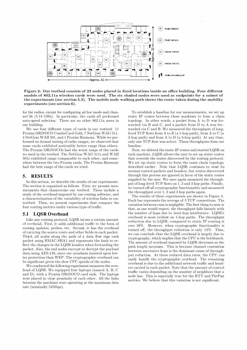
4. TESTBEDThe experimental data reported in this paper are the re-

sults of measurements we have taken on a 23-node wirelesstestbed. Our testbed is located on one floor of a fairly typicaloffice building, with the nodes placed in offices, conferencerooms and labs. Unlike wireless-friendly cubicle environ-ments, our building has rooms with floor-to-ceiling walls andsolid wood doors. With the exception of one additional lap-top used in the mobility experiments, the nodes are locatedin fixed locations and did not move during testing. The node

density was deliberately kept high enough to enable a widevariety of multi-hop path choices. See Figure 2.

The nodes are primarily laptop PCs with Intel PentiumII processors with clock rates from 233 to 300 MHz, butalso included a couple slightly faster laptops as well as twodesktop machines. All of the nodes run Microsoft WindowsXP. The TCP stack included with XP supports the SACKoption by default, and we left it enabled for all of our TCPexperiments. All of our experiments were conducted overIPv4 using statically assigned addresses. Each node has an802.11a PCCARD radio. We used the default configuration



0 1

0 4

1 3

0 0

0 0

0 0

0 0

P r o x i m O R i N O C O

P r o x i m H a r m o n y

N e t G e a r W A B 5 0 1

N e t G e a r W A G 5 1 1

0 5

0 7

1 0

1 6

2 0

2 2

2 4

2 5

5 9

6 5

6 7

1 0 0 1 2 8

2 3

5 4 5 5 5 6

6 4

6 6

6 8

A p p r o x . 6 1 m

A

p

p

r

o

x

.

3

2

m

M o b i l e n o d e w a l k i n g p a t h

Figure 2: Our testbed consists of 23 nodes placed in fixed locations inside an office building. Four differentmodels of 802.11a wireless cards were used. The six shaded nodes were used as endpoints for a subset of the experiments (see section 5.3). The mobile node walking path shows the route taken during the mobilityexperiments (see section 6).

for the radios, except for configuring ad hoc mode and chan-nel 36 (5.18 GHz). In particular, the cards all performedauto-speed selection. There are no other 802.11a users inour building.

We use four different types of cards in our testbed: 11Proxim ORiNOCO ComboCard Gold, 7 NetGear WAG 511,4 NetGear WAB 501, and 1 Proxim Harmony. While we per-formed no formal testing of radio ranges, we observed thatsome cards exhibited noticeably better range than others.The Proxim ORiNOCOs had the worst range of the cardswe used in the testbed. The NetGear WAG 511s and WAB501s exhibited range comparable to each other, and some-where between the two Proxim cards. The Proxim Harmonyhad the best range of the cards we tried.

5. RESULTSIn this section, we describe the results of our experiments.

The section is organized as follows. First, we present mea-surements that characterize our testbed. These include astudy of the overhead imposed by our routing software, anda characterization of the variability of wireless links in ourtestbed. Then, we present experiments that compare thefour routing metrics under various type of traffic.

5.1 LQSR OverheadLike any routing protocol, LQSR incurs a certain amount

of overhead. First, it adds additional traffic in the form of routing updates, probes, etc. Second, it has the overheadof carrying the source route and other fields in each packet.Third, all nodes along the path of a data flow sign eachpacket using HMAC-SHA1 and regenerate the hash to re-

flect the changes in the LQSR headers when forwarding thepacket. Also, the end nodes encrypt or decrypt the payloaddata using AES-128, since our sysadmin insisted upon bet-ter protection than WEP. The cryptographic overhead canbe significant given the slow CPU speeds of the nodes.

We conducted the following experiment measures the over-head of LQSR. We equipped four laptops (named A, B, Cand D), with a Proxim ORiNOCO card each. The laptopswere placed in close proximity of each other. All the linksbetween the machines were operating at the maximum datarate (nominally 54Mbps).

To establish a baseline for our measurements, we set upstatic IP routes between these machines to form a chaintopology. In other words, a packet from A to D was for-warded via B and C, and a packet from D to A was for-warded via C and B. We measured the throughput of long-lived TCP flows from A to B (a 1-hop path), from A to C (a2-hop path) and from A to D (a 3-hop path). At any time,only one TCP flow was active. These throughputs form ourbaseline.

Next, we deleted the static IP routes and started LQSR oneach machine. LQSR allows the user to set up static routesthat override the routes discovered by the routing protocol.We set up static routes to form the same chain topologydescribed earlier. Note that LQSR continues to send itsnormal control packets and headers, but routes discoveredthrough this process are ignored in favor of the static routessupplied by the user. We once again measured the through-

put of long-lived TCP flows on 1, 2 and 3 hop paths. Finally,we turned off all cryptographic functionality and measuredthe throughput over 1, 2 and 3 hop paths again.

The results of these experiments are shown in Figure 3.Each bar represents the average of 5 TCP connections. Thevariation between runs is negligible. The first thing to note isthat, as one would expect, the throughput falls linearly withthe number of hops due to inter-hop interference. LQSR’soverhead is most evident on 1-hop paths. The throughputreduction due to LQSR, compared to static IP routing isover 38%. However, when cryptographic functionality isturned off, the throughput reduction is only 13%. Thus,we can conclude that the LQSR overhead is largely due tocryptography, which implies that the CPU is the bottleneck.The amount of overhead imposed by LQSR decreases as the

path length increases. This is because channel contentionbetween successive hops is the dominant cause of through-put reduction. At these reduced data rates, the CPU caneasily handle the cryptographic overhead. The remainingoverhead is due to the additional network traffic and head-ers carried in each packet. Note that the amount of controltraffic varies depending on the number of neighbors that anode has. This is especially true for the RTT and PktPairmetrics. We believe that this variation is not significant.



0

2000

4000

6000

8000

10000

12000

14000

16000

1 2 3Number of Hops

A v e r a g e

T C P T h r o u g

h p u

t ( K b p s

)Static IP

MCL No Crypto

MCL With Crypto

Figure 3: MCL overhead is not significant on multi-hop paths.

5.2 Link Variability in the TestbedIn our testbed, we allow the radios to dynamically select

their own data rates. Thus, different links in our testbedhave different bandwidths. To characterize this variability inlink quality, we conducted the following experiment. Recallthe PktPair metric collects a sample of the amount of timerequired to transmit a probe packet every 2 seconds on eachlink. We modified the implementation of the PktPair metricto keep track of the minimum sample out of every successive

50 samples (i.e minimum of samples 1-50, then minimum of samples 51-100 etc.). We divide the size of the second packetby this minimum. The resulting number is an indication of the bandwidth of that link during that 100 second period.In controlled experiments, we verified that this approachapproximates the raw link bandwidth. We gathered thesesamples from all links for a period of 14 hours. Thus, foreach link there were a total of 14 × 60 × 60 ÷ 100 = 504bandwidth samples. There was no traffic on the testbedduring this time. We discard any intervals in which thecalculated bandwidth is more than 36Mbps, which is thehighest data rate that we actually see in the testbed. Thisresulted in removal of 3.83% of all bandwidth samples. Still,the resulting number is not an exact measure of the availablebandwidth, since it is difficult to correctly account for alllink-layer overhead. However, we believe that the number isa good (but rough) indication of the link bandwidth duringthe 100 second period.

Of the 23 × 22 = 506 total possible links, only 183 linkshad non-zero average bandwidth, where the average wascomputed across all samples gathered over 14 hours. Wefound that bandwidths of certain links varied significantlyover time, while other links it was relatively stable. Exam-ples of two such links appear in Figures 4 and 5. In the firstcase, we see that the bandwidth is relatively stable over theduration of the experient. In the second case, however, thebandwidth is much more variable. Since the quality of linksin our testbed varies over time, we are careful to repeat ourexperiments at different times.

In Figure 6 we compare the bandwidth on the forwardand reverse direction of a link. To do this, we consider allpossible unordered node pairs. The number of such pairs is23× 22÷ 2 = 253. Each pair corresponds to two directionallinks. Each of these two links has its own average band-width. Thus, each pair has two bandwidths associated withit. Out of the 253 possible node pairs, 90 node pairs hadnon-zero average bandwidth in both forward and reverse di-rections. In Figure 6, we plot a point for each such pair.The X-coordinate of the pair represents the link with thelarger bandwidth. The existence of several points below the

diagonal line implies that there are several pairs for whichthe forward and the reverse bandwidths differ significantly.In fact, in 47 node pairs, the forward and the reverse band-widths differ by more than 25%.

5.3 Impact on Long Lived TCP FlowsHaving characterized the overhead of our routing software,

and the quality of links in our testbed, we can now discuss

how various routing metrics perform in our testbed. Webegin by discussing the impact of routing metrics on theperformance of long-lived TCP connections. In today’s In-ternet, TCP carries most of the traffic, and most of the bytesare carried as part of long-lived TCP flows [13]. It is rea-sonable to expect that similar types of traffic will be presenton community networks, such as [6, 27]. Therefore, it isimportant to examine the impact of routing metrics on theperformance of long-lived TCP flows.

We start the performance comparison with a simple exper-iment. We carried out a TCP transfer between each uniquesender-destination pair. There are 23 nodes in our testbed,so a total of 23× 22 = 506 TCP transfers were carried out.Each TCP transfer lasted for 3 minutes, and transferred asmuch data as it could. On the best one-hop path in our

testbed a 3 minute connection will transfer over 125MB of data. Such large TCP transfers ensure repeatability of re-sults. We had previously determined empirically that TCPconnections of 1 minute duration were of sufficient length toovercome startup effects and give reproducible results. Weused 3 minute transfers in these experiments, to be conser-vative. We chose to fix the transfer duration, instead of theamount of data transferred, to keep the running time of eachexperiment predictable. Only one TCP transfer was activeat any time. The total time required for the experiment was just over 25 hours. We repeated the experiment for eachmetric.

In Figure 7 we show the median throughput of the 506TCP transfers for each metric. We choose median to repre-sent the data instead of the mean because the distribution(which includes transfers of varying path lengths) is quiteskewed. The height error bars represent the semi-inter quar-tile range (SIQR), which is defined as half the difference be-tween 25th and 75th percentile of the data. SIQR is the rec-ommended measure of dispersion when the central tendencyof the data is represented by the median [14]. Since eachconnection is run between a different pair of nodes the rela-tively large error bars indicate that we observe a wide rangeof throughputs across all the pairs. The median through-put using the HOP metric is 1100Kbps, while the medianthroughput using the ETX metric is 1357Kbps. This repre-sents an improvement of 23.1%.

In contrast, De Couto et al. [9] observed almost no im-provement for ETX in their DSR experiments. There are

several possible explanations for this. First, they used UDPinstead of TCP. A bad path will have more impact on thethroughput of a TCP connection (due to window backoffs,timeouts etc.) than on the throughput of a UDP connec-tion. Hence, TCP amplifies the negative impact of poorroute selection. Second, in their testbed the radios were setto their lowest sending rate of 1Mbps, whereas we allow theradios to set transmit rates automatically (auto-rate). Webelieve links with lower loss rates also tend to have higherdata rates, further amplifying ETX’s improvement. Third,our testbed has 6-7 hop diameter whereas their testbed has



0

5000

10000

15000

20000

25000

30000

35000

0 2 4 6 8 10 12 14

B a n d w i d t h ( K b p s )

Time (Hours)

From 65 to 100

Figure 4: The bandwidth of thelink from node 65 to node 100 isrelatively stable.

0

5000

10000

15000

20000

25000

30000

35000

0 2 4 6 8 10 12 14

B a n d w i d t h ( K b p s )

Time (Hours)

From 68 to 66

Figure 5: The bandwidth of thelink from node 68 to node 66 variesover time.

0

5

10

15

20

25

30

0 5 10 15 20 25 30

A v g .

B a n d w i d t h ( M b p s )

Avg. Bandwidth (Mbps)

Figure 6: For many node pairs,the bandwidths of the two links be-tween the nodes is unequal.

0

500

1000

1500

2000

HOP ETX RTT PktPair

T h r o u g h p u t ( K b p s )

Metric

Figure 7: All pairs: Medianthroughput of TCP transfer.

0

5

10

15

20

25

30

HOP ETX RTT PktPair

N u m b e r o f P a t h s

Metric

Figure 8: All Pairs: Median num-ber of paths per TCP transfer.

0

1

2

3

4

5

6

HOP ETX RTT PktPair

P a t h L e n g t h ( H o p s )

Metric

Figure 9: All pairs: Median pathlength of a TCP transfer.

0

1

2

3

4

5

6

7

8

0 1 2 3 4 5 6 7 8

P a t h L e n g t h u n d e r E T X

Path Length under HOP

Figure 10: All Pairs: Comparison of HOP andETX path lengths. ETX consistently uses longerpaths than HOP.

a 5-hop diameter [8]. As we discuss below, ETX’s improve-ment over HOP is more pronounced at longer path lengths.

The RTT metric gives the worst performance among thefour metrics. This is due to the phenomenon of self-interferencethat we previously noted in Section 2.2. The phenomenonmanifests itself in the number of paths taken by the connec-tion. At the beginning the connection uses a certain path.However, due to self-interference, the metric on this pathsoon rises. The connection then chooses another path. Thisis illustrated in Figure 8. The graph shows the median num-

ber of paths taken by a connection. The RTT metric usesfar more paths per connection than other metrics. The HOPmetric uses the least number of paths per connection - themedian is just 1.

The PktPair metric performs better than RTT, but worsethan both HOP and ETX. This is again due to the phe-nomenon of self-interference. While the RTT metric suffersfrom self-interference on all hops along the path, the PktPairmetric eliminates the self-interference problem on the firsthop. The impact of this can be seen in the median numberof paths (12) tried by a connection using the PktPair met-

ric. This number is lower than median using RTT (20.5),but substantially higher than HOP and ETX.

Note that the ETX metric also uses several paths per con-nection: the median is 4. This is because for a given nodepair, multiple paths that are essentially equivalent can ex-ist between them. There are several such node pairs in ourtestbed. Small fluctuations in the metric values of equiv-alent paths can make ETX choose one path over another.We plan to investigate route damping strategies to alleviatethis problem.

The self-interference, and consequent route flapping ex-perienced the RTT metric has also been observed in wirednetworks [18, 2]. In [18], the authors propose to solve theproblem by converting the RTT to utilization, and normal-izing the resulting value for use as a route metric. In [2], theauthors propose to use hysteresis to alleviate route flapping.We are currently investigating these techniques further. Ourinitial results show that hysteresis may reduce the severityof the problem, but not significantly so.

5.4 Impact of Path LengthThe HOP metric produces significantly shorter paths than

the three other metrics. This is illustrated in Figure 9. Thebar chart shows the median across all 506 TCP transfers

of the average path length of each transfer. To calculatethe average path length of a TCP transfer, we keep trackof the paths taken by all the data-carrying packets in thetransfer. We calculate the average path length by weightingthe length of each unique path by the number of packets thattook that path. The error bars represent SIQR. The HOPmetric has the shortest median path length (2), followed byETX (3.01), RTT (3.43) and PktPair (3.58).

We now look at ETX and HOP path lengths in more de-tail. In Figure 10, we plot the average path length of eachTCP transfer using HOP versus the average path length



0

2000

4000

6000

8000

10000

12000

0 1 2 3 4 5 6 7 8


Average Path Length

Figure 11: All Pairs: Throughputas a function of path length underHOP. The metric does a poor jobof selecting multi-hop paths.

0

2000

4000

6000

8000

10000

12000

0 1 2 3 4 5 6 7 8


Average Path Length

Figure 12: All Pairs: Throughputas a function of path length underETX. The metric does a better jobof selecting multi-hop paths.

0

2000

4000

6000

8000

10000

12000

0 1 2 3 4 5 6 7 8


Average Path Length

Figure 13: All Pairs: Throughputas a function of path length underRTT. The metric does a poor jobof selecting even one hop paths.

0

2000

4000

6000

8000

10000

12000

0 1 2 3 4 5 6 7 8


Average Path Length

Figure 14: All Pairs: Throughput as a functionof path length under PktPair. The metric findsgood one-hop paths, but poor multi-hop paths.

using ETX. Again, the ETX metric produces significantlylonger paths than the HOP metric. The testbed diameter is7 hops using ETX and 6 hops using HOP.

We also examined the impact of average path length onTCP throughput. In Figure 11 we plot the throughputof a TCP connection against its path length using HOPwhile in Figure 12 we plot the equivalent data for ETX.First, note that as one would expect, longer paths pro-duce lower throughputs because channel contention keepsmore than one link from being active. Second, note thatETX’s higher median throughput derives more from avoid-ing lower throughputs than from achieving higher through-puts. Third, ETX does especially well at longer path lengths.The ETX plot is flat from around 5 through 7 hops, possiblyindicating that links at opposite ends of the testbed do notinterfere. Fourth, ETX avoids poor one-hop paths whereasHOP blithely uses them.

We now look at the performance of RTT and PktPair inmore detail. In Figure 13 we plot TCP throughput versus

average path length for RTT while in Figure 14 we plot thedata for PktPair. RTT’s self-interference is clearly evidentin the low throughputs and high number of connections withaverage path lengths between 1 and 2 hops. With RTT, even1-hop paths are not stable. In contrast, with PktPair the1-hop paths look good (equivalent to ETX in Figure 12) butself-interference is evident starting at 2 hops.

5.5 Variability of TCP ThroughputTo measure the impact of routing metrics on the variabil-

ity of TCP throughput, we carry out the following experi-

ment. We select 6 nodes on the periphery of the testbed, asshown in Figure 2. Each of the 6 nodes then carried out a3-minute TCP transfer to the remaining 5 nodes. The TCPtransfers were set sufficiently apart to ensure that no morethan one TCP transfer will be active at any time. There isno other traffic in the testbed. We repeated this experiment

10 times. Thus, there were a total of 6× 5× 10 = 300 TCPtransfers. Since each transfer takes 3 minutes, the experi-ment lasts for over 15 hours.

In Figure 15 we show the median throughput of the 300TCP transfers using each metric. As before, the error barsrepresent SIQR. Once again, we see that the RTT metric isthe worst performer, and the ETX metric outperforms theother three metrics by a wide margin.

The median throughput using the ETX metric is 1133Kbps,while the median throughput using the HOP metric is 807.5.This represents a gain of 40.3%. This gain is higher than the23.15% obtained in the previous experiment because thesemachines are on the periphery of the network, and thus, thepaths between them tend to be longer. As we have noted in

Section 5.4, the ETX metric tends to perform better thanHOP on longer paths. The higher median path lengths sub-stantially degrades the performance of RTT and PktPair,compared to their performance shown in Figure 7.

The HOP metric selects the shortest path between a pairof nodes. If multiple shortest paths are available, the met-ric simply chooses the first one it finds. This introducesa certain amount of randomness in the performance of theHOP metric. If multiple TCP transfers are carried out be-tween a given pair of nodes, the HOP metric may selectdifferent paths for each transfer. The ETX metric, on theother hand, selects “good” links. This means that it tendsto choose the same path between a pair of nodes, as longas the link qualities do not change drastically. Thus, if sev-eral TCP transfers are carried out between the same pair of

nodes at different times, they should yield similar through-put using ETX, while the throughput under HOP will bemore variable. This fact is illustrated in Figure 16.

The figure uses coefficient of variation (CoV) as a measureof variability. CoV is defined as standard deviation dividedby mean. There is one point in the figure for each of the 30source-destination pairs. The X-coordinate represents CoVof the throughput of 10 TCP transfers conducted betweena given source-destination pair using ETX, and the Y co-ordinate represents the CoV using HOP. The CoV values are



0

300

600

900

1200

1500

HOP ETX RTT PktPair


Metric

Figure 15: 30 Pairs: Median throughput with dif-ferent metrics.

significantly lower with ETX. Note that a single point lieswell below the diagonal line, indicating that HOP providedmore stable throughput than ETX. This point representsTCP transfers from node 23 to node 10. We are currentlyinvestigating these transfers further. It is interesting to notethat for the reverse transfers, i.e. from node 10 to node 23,ETX provides lower CoV than than HOP.

5.6 Multiple Simultaneous TCP Transfers

In the experiments described in the previous section, onlyone TCP connection was active at any time. This is un-likely to be the case in a real network. In this section, wecompare the performance of ETX, HOP and PktPair formultiple simultaneous TCP connections. We do not con-sider RTT since its performance is poor even with a singleTCP connection.

We use the same set of 6 peripheral nodes shown in Fig-ure 2. We establish 10 TCP connections between each dis-tinct pair of nodes. Thus, there are a total of 6×5×10 = 300possible TCP connections. Each TCP connection lasts for3 minutes. The order in which the connections are estab-lished is randomized. The wait time between the start of two successive connections determines the number of simul-taneously active connections. For example, if the wait timebetween starting consecutive connections is 90 seconds, thentwo connections will be active simultaneously. We repeatthe experiment for various numbers of simultaneously ac-tive connections.

For each experiment we calculate the median throughoutof the 300 connections, and multiply it by the number of simultaneously active connections. We call this product theMultiplied Median Throughput (MMT). MMT should in-crease with the number of simultaneous connections, untilthe load becomes too high for the network to carry.

In Figure 17 we plot MMT against the number of simul-taneous active connections. The figure shows that the per-formance of the PktPair metric gets significantly worse asthe the number of simultaneous connections increase. This

is because the self-interference problem gets worse with in-creasing load. In the case of ETX, the MMT increases toa peak at 5 simultaneous connections. The MMT growthis significantly less than linear because there is not muchparallelism in our testbed (many links interfere with eachother) and the increase that we are seeing is partly becausea single TCP connection does not fully utilize the end-to-end path. We believe the MMT falls beyond 5 simultaneousconnections due to several factors, including 802.11 MACinefficiencies and instability in the ETX metric under veryhigh load. The MMT using HOP deteriorates much faster

0

0.2

0.4

0.6

0.8

1

0 0.2 0.4 0.6 0.8 1

H O P T h r o u g h p u t C o V

ETX Throughput CoV

Figure 16: 30 Pairs: The lower CoVs under ETXindicate that ETX chooses stable links.

0

200

400

600

800

1000

1200

1400

1600

1800

1 2 3 4 5 6 9 18

Number of simultaneous TCP connections

N o r m a

l i z e

d T h r o u g

h p u

t ( K b p s

)

H OP E TX P kt Pa ir

Figure 17: Throughputs with multiple simulta-neous TCP connections.

than it does with ETX. As discussed in Section 5.8, at higherloads HOP performance drops because link-failure detectionbecomes less effective.

5.7 Web-like TCP TransfersWeb traffic constitutes a significant portion of the total

Internet traffic today. It is reasonable to assume that webtraffic will also be a significant portion of traffic in wirelessmeshes such as the MIT Roofnet [26]. The web traffic ischaracterized by the heavy-tailed distribution of flow sizes:most transfers are small, but there are some very large trans-fers [21]. Thus, it is important to examine the performanceof web traffic under various routing metrics.

To conduct this experiment, we set up a web server on host128. The six peripheral nodes served as web clients. Theweb traffic was generated using Surge [5]. The Surge soft-ware has two main parts, a file generator and a request gen-erator. The file generator generate files of varying sizes thatare placed on the web server. The Surge request generatormodels a web user that fetches these files. The file generatorand the request generator offer a large number of parametersto customize file size distribution and user behaviors. Weran Surge with its default parameter settings, which have

been derived through modeling of empirical data [5].Each Surge client modeled a single user running HTTP 1.1

Each user session lasted for 40 minutes, divided in four slotsof 10 minutes each. Each user fetched over 1300 files fromthe web server. The smallest file fetched was 77 bytes long,while the largest was 700KB. We chose to have only oneclient active at any time, to allow us to study the behaviorof each client in detail. We measure the latency or eachobject: the amount of time elapsed between the request foran object, and the completion of its receipt. Note that weare ignoring any rendering delays.



0

5

10

15

20

25

30

1 10 20 23 68 100

Host

M e

d i a n

L a

t e n c y

( m s

)

HOP ETX

Figure 18: Median latency for allfiles fetched

0

2

4

6

8

10

12

14

16

1 10 20 23 68 100

Host

M e

d i a n

L a

t e n c y

( m s

)

HOP ETX

Figure 19: Median latency for filessmaller than 1KB

0

20

40

60

80

100

120

140

160

180

1 10 20 23 68 100

Host

M e

d i a n

L a

t e n c y

( m s

)

HOP ETX

Figure 20: Median latency for fileslarger than 8KB

In Figure 18, we plot the median latencies experiencedby each client. It can be seen that ETX reduces the laten-cies observed by clients that are further away from the webserver. This is consistent with our earlier finding ETX tendsto perform better than HOP on longer paths. For host 23,100 and 20, the median latency under ETX is almost 20%lower than the median latency under HOP. These hosts arerelatively further away from the webserver running on host128. On the other hand, for host 1, the median latency un-der HOP is lower by 20%. Host 1 is just one hop away from

the web server. These results are consistent with the resultsin Section 5.4: on longer paths, ETX performs better thanHOP, but on one-hop paths, the HOP metric sometimesperforms better.

To study whether the impact of ETX is limited to largetransfers we studied the median response times for small ob- jects, i.e. files that are less than 1KB in size and large ob- jects, i.e., those over 8KB in size. These medians are shownin Figures 19 and 20, respectively. The benefit of ETX isindeed more evident in case of larger transfers. However,ETX also reduces the latency of small transfers by signifi-cant proportion. This is particularly interesting as the datasent from the server to client in such small transfers fits in-side a single TCP packet. It is clear that even for such short

transfers, the paths selected by ETX are better.

5.8 DiscussionWe conclude from our results that load-sensitivity is the

primary factor determining the relative performance of thethree metrics. The RTT metric is the most sensitive toload; it suffers from self-interference even on one-hop pathsand has the worst performance. The PktPair metric is notaffected by load generated by the probing node, but it issensitive to other load on the channel. This causes self-interference on multi-hop paths and degrades performance.The ETX metric has the least sensitivity to load and it per-forms the best.

Our experience with HOP leads us to believe that its per-

formance is very sensitive to competing factors controllingthe presence of poor links in the link cache. Consider theevolution of a route during a long data transfer. Whenthe transfer starts, the link cache contains a fairly com-plete topology, including many poor links. The shortest-path Dijkstra computation picks a route that probably in-cludes poor (lossy or slow) links. Then as the data transferproceeds, Route Maintenance detects link failures and sendsRoute Error messages, causing the failed link to be removedfrom link caches. Since poor links suffer link failures morefrequently than good links, over time the route tends to im-

0

100

200

300

400

500

600

HOP ETX

Metric

M e d i a n T C P T h r o u g h p u t ( K b p s )

Figure 21: Median Throughput of 45 1-minute TCPtransfers with mobile sender using HOP and ETX.

prove. However this process can go too far: if too manylinks are removed, the route can get longer and longer untilfinally there is no route left and the node performs RouteDiscovery again. On the other hand, a background load of unrelated traffic in the network tends to repopulate the linkcache with good and bad links, because of the caching of linkexistence from overheard or forwarded packets. The compe-tition between these two factors, one removing links from thelink cache and the other adding links, controls the qualityof the HOP metric’s routes. For example, originally LQSRsent Link Info messages when using HOP. When we changedthat, to make LQSR with HOP behave more like DSR, wesaw a significant improvement in median TCP throughput.This is because the background load of Link Info messageswas repopulating the link caches too quickly, reducing theeffectiveness of the Route Error messages.

Our study has several limitations that we would like tocorrect in future work. First, our data traffic is entirelyartificial. We would prefer to measure the p erformance of real network traffic generated by real users. Second, we donot investigate packet loss and jitter with constant-bit-ratedatagram traffic. This would be relevant to the performanceof multimedia traffic. We would also like to investigate per-formance of other wireless link quality metrics such as signalstrength.

6. A MOBILE SCENARIOIn the traffic scenarios that we have considered so far,

all the nodes have been stationary. In community networkslike [6, 27, 26] most nodes are indeed likely to be station-ary. However, in most other ad hoc wireless networks, atleast some of the nodes are mobile. Here, we consider a sce-nario that involves a single mobile node, and compare theperformance of ETX and HOP metrics.

The layout of our testbed is shown in Figure 2. We set upa TCP receiver on node 100. We slowly and steadily walked



around the periphery of the network with a Dell LatitudeLaptop, equipped with a NetGear card. A process runningon this laptop repeatedly established a TCP connection tothe receiver running on node 100, and transferred as muchdata as it could in 1 minute. We did 15 such transfers ineach walk-about. We did 3 such walk-abouts each for ETXand HOP. Thus, for each metric we did 45 TCP transfers.

The median throughput of these 45 transfers, along withSIQR is shown in Figure 21. We choose median over mean

since the distribution of throughputs is highly skewed. Themedian throughput under HOP metric is 36% higher thanthe median throughput under the ETX metric. Note alsothat the SIQR for ETX is 173, which is comparable to theSIQR of 188 for HOP. Since the median throughput underETX is lower, the higher SIQR indicates greater variabilityin throughput under ETX.

As the sender moves around the network, the ETX met-ric does not react sufficiently quickly to track the changes inlink quality. As a result, the node tries to route its packetsusing stale, and sometimes incorrect information. The sal-vaging mechanisms built into LQSR do help to some extent,but not well enough to overcome the problem completely.Our results with PktPair (not included here) indicate that

that this problem is not limited to just the ETX metric.Any approach that tries to measure link quality will needsome time to come up with a stable measure of link quality.If during this time the mobile user moves sufficiently, thelink quality measurements would not be correct. Note thatwe do have penalty mechanisms built into our link qual-ity measurements. If a data packet is dropped on a link,we penalize the metric as described in Section 2. We areinvestigating the possibility that by penalizing the metricmore aggressively on data packet drops we can improve theperformance of ETX.

The HOP metric, on the other hand, faces no such prob-lems. It uses new links as quickly as the node discoversthem. The efficacy of various DSR mechanisms to improveperformance in a mobile environment has been well docu-

mented [15]. The metric also removes from link cache anylink on which a node suffers even one packet loss. This mech-anism, which hurts the performance of HOP metric underheavy load, benefits it in the mobile scenario.

We stress that this experiment is not an attempt to drawgeneral conclusions about the suitability of any metric forrouting in mobile wireless networks. Indeed, such conclu-sions can not be drawn from results of a single experiment.This experiment only serves to underscore the fact thatstatic and mobile wireless networks can present two verydifferent sets of challenges, and solutions that work well inone setting are not guaranteed to work just as well in an-other.

7. RELATED WORKThere is a large body literature comparing the perfor-mance of various ad hoc routing protocols. Most of thiswork is simulation-based and the ad hoc routing protocolsstudied all minimize hop-count. Furthermore, many of thesestudies focus on scenarios that involve significant node mo-bility. For example, Broch et al. [7] compared the perfor-mance of DSDV [23], TORA [22], DSR [15], and AODV [24]via simulations.

The problem of devising a link-quality metric for static80.211 ad hoc networks has been studied previously. Most

notably, De Couto et al. [9] propose ETX and compare itsperformance to HOP using DSDV and DSR with a small-datagram workload. Their study differs from ours in manyaspects. They conclude that ETX outperforms HOP withDSDV, but find little benefit with DSR. They only studythe throughput of single, short (30 second) data transfersusing small datagrams. Their experiments include no mo-bility. In contrast, we study TCP transfers. We examinethe impact of multiple simultaneous data transfers. We

study variable-length data transfers and in particular, lookat web-like workloads where latency is more important thanthroughput. Finally, our work includes a scenario with somemobility. Their implementation of DSR differs from ours inseveral ways, which may partly explain our different results.They do not have Metric Maintenance mechanisms. In theirtestbed (as in ours), the availability of multiple paths meansafter the initial route discovery the nodes rarely send RouteRequests. Hence during their experiments, the sender effec-tively routes using a snapshot of the ETX metrics discoveredat the start of the experiment. Their implementation takesadvantage of 802.11 link-layer acknowledgments for failuredetection. This means their link-failure detection is not vul-nerable to loss, or perceived loss due to delay. Their imple-

mentation does not support salvaging. They mitigate thisin their experiments by sending five “priming” packets be-fore starting each data transfer. Their implementation usesa “blacklist” mechanism to cope with asymmetric links. Fi-nally, their implementation has no security support and doesnot use cryptography so it has much less CPU overhead.

Woo et al. [28] examines the interaction of link quality andad hoc routing for sensor networks. Their scheme is basedon passive observation of packet reception probability. Usingthis probability, they compare several routing protocols in-cluding shortest-path routing with thresholding to eliminatelinks with poor quality and ETX-based distance-vector rout-ing. Their study uses rate-limited datagram traffic. Theyconclude that ETX-based routing is more robust.

Signal-to-noise ratio (SNR), has been used as a link qual-

ity metric in several routing schemes for mobile ad hoc net-works. For example, in [12] the authors use an SNR thresh-old value to filter links discovered by DSR Route Discovery.The main problem with these schemes is that they may endup excluding links that are necessary to maintain connec-tivity. Another approach is used in [11], where links are stillclassified as good and bad based on a threshold value, buta path is permitted to use poor-quality links to maintainconnectivity. Punnoose et. al. [25] also use signal strengthas a link quality metric. They convert the predicted sig-nal strength into a link quality factor, which is used as-sign weights to the links. Zhao and Govindan [29]. studiedpacket delivery performance in sensor networks, and discov-ered that high signal strength implies low packet loss, butlow signal strength does not imply high packet loss. We planto study the SNR metric in our testbed as part of our futurework. Our existing hardware and software setup does notprovide adequate support to study this metric.

Awerbuch et. al. [4] study impact of automatic rate se-lection on performance of ad hoc networks. They propose arouting algorithm that selects a path with minimum trans-mission time. Their metric does not take packet loss intoaccount. It is possible to combine this metric with the ETXmetric, and study performance of the combined metric. Thisis also part of our future work.



An implementation of AODV that uses the link-filteringapproach, based on measurement of loss rate of unicast probes,was demonstrated in a recent IETF meeting [3, 19]. We planto test this implementation in our testbed.

8. CONCLUSIONSWe have examined the performance of three candidate

link-quality metrics for ad hoc routing and compared them

to minimum hop-count routing. Our results are based onseveral months of experiments using a 23-node static ad hocnetwork in an office environment. The results show thatwith stationary nodes the ETX metric significantly outper-forms hop-count. The RTT and PktPair metrics p erformpoorly because they are load-sensitive and hence suffer fromself-interference. However, in a mobile scenario hop-countperforms b etter because it reacts more quickly to fast topol-ogy change.

Acknowledgments

Yih-Chun Hu implemented DSR within the MCL frameworkas part of his internship project. This was our starting point

for developing LQSR. We would like to thank Atul Adya,Victor Bahl and Alec Wolman for several helpful discussionsand suggestions. We would also like to thank the anonymousreviewers for their feedback. Finally, we would like to thankthe support staff at Microsoft Research for their help withvarious system administration issues.

9. REFERENCES

[1] A. Adya, P. Bahl, J. Padhye, A. Wolman, andL. Zhou. A multi-radio unification protocol for IEEE802.11 wireless networks. In BroadNets, 2004.

[2] D. G. Andersen, H. Balakrishnan, M. F. Kaashoek,and R. Morris. Resilient overlay networks. In SOSP ,

2001.[3] AODV@IETF. http://moment.cs.ucsb.edu/aodv-ietf/.

[4] B. Awerbuch, D. Holmer, and H. Rubens. Highthroughput route selection in mult-rate ad hocwireless networks. Technical report, Johns Hopkins CSDept, March 2003. v 2.

[5] P. Bardford and M. Crovella. Generatingrepresentative web workloads for network and serverperformance evaluation. In SIGMERICS , Nov. 1998.

[6] Bay area wireless users group.http://www.bawug.org/.

[7] J. Broch, D. Maltz, D. Johnson, Y.-C. Hu, andJ. Jetcheva. A performance comparison of multi-hopwireless ad hoc network routing protocols. InMOBICOM , Oct. 1998.

[8] D. De Couto. Personal communication, Nov. 2003.

[9] D. De Couto, D. Aguayo, J. Bicket, and R. Morris.High-throughput path metric for multi-hop wirelessrouting. In MOBICOM , Sep 2003.

[10] R. Draves, J. Padhye, and B. Zill. The architecture of the Link Quality Source Routing Protocol. TechnicalReport MSR-TR-2004-57, Microsoft Research, 2004.

[11] T. Goff, N. Abu-Aahazaleh, D. Phatak, andR. Kahvecioglu. Preemptive routing in ad hocnetworks. In MOBICOM , 2001.

[12] Y.-C. Hu and D. B. Johnson. Design anddemonstration of live audio and video over multi-hopwireless networks. In MILCOM , 2002.

[13] P. Huang and J. Heidemann. Capturing tcp burstinessfor lightweight simulation. In SCS Multiconference on

Distributed Simulation , Jan. 2001.

[14] R. Jain. The Art of Computer Systems PerformanceAnalysis. John Wiley and Sons, Inc., 1991.

[15] D. B. Johnson and D. A. Maltz. Dynamic sourcerouting in ad-hoc wireless networks. In T. Imielinskiand H. Korth, editors, Mobile Computing . KluwerAcademic Publishers, 1996.

[16] R. Karrer, A. Sabharwal, and E. Knightly. EnablingLarge-scale Wireless Broadband: The Case for TAPs.In HotNets, Nov 2003.

[17] S. Keshav. A Control-theoretic approach to flowcontrol. In SIGCOMM , Sep 1991.

[18] A. Khanna and J. Zinky. The Revised ARPANETRouting Metric. In SIGCOMM , 1989.

[19] L. Krishnamurthy. Personal communication, Dec.2003.

[20] J. Moy. OSPF Version 2. RFC2328, April 1998.

[21] K. Park, G. Kim, and M. Crovella. On therelationship between file sizes, transport protocols andself-similar network tarffic. In ICNP , 1996.

[22] V. D. Park and M. S. Corson. A highly adaptivedistributed routing algorithm for mobile wirelessnetworks. In INFOCOM , Apr 1997.

[23] C. E. Perkins and P. Bhagwat. Highly dynamicdestination-sequenced distance vector routing (dsdv)for mobile computeres. In SIGCOMM , Sep. 1994.

[24] C. E. Perkins and E. M. Royer. Ad-hoc on-demanddistance vector routing. In WMCSA, Feb 1999.

[25] R. Punnose, P. Nitkin, J. Borch, and D. Stancil.Optimizing wireless network protocols using real timepredictive propagation modeling. In RAWCON , Aug1999.

[26] MIT roofnet. http://www.pdos.lcs.mit.edu/roofnet/.[27] Seattle wireless. http://www.seattlewireless.net/.

[28] A. Woo, T. Tong, and D. Culler. Taming theunderlying challenges of reliable multihop routing insensor networks. In SenSys, Nov 2003.

[29] J. Zhao and R. Govindan. Understanding packetdelivery performance in dense wireless sensornetworks. In SenSys, Nov. 2003.

Comparison of Routing Metrics

Documents

Transcript of Comparison of Routing Metrics