Comparison of reduced- and full-space algorithms for

PDE-constrained optimization

Jason E. Hicken�

Rensselaer Polytechnic Institute, Troy, New York, 12180

Juan J. Alonsoy

Stanford University, Stanford, California 94305-3030

PDE-constrained optimization problems are often solved using reduced-space quasi-Newton algorithms. Quasi-Newton methods are e�ective for problems with relatively fewdegrees of freedom, but their performance degrades as the problem size grows. In thispaper, we compare two inexact-Newton algorithms that avoid the algorithmic scaling is-sues of quasi-Newton methods. The two inexact-Newton algorithms are distinguished byreduced-space and full-space implementations. Numerical experiments demonstrate thatthe full-space (or one-shot) inexact-Newton algorithm is typically the most e�cient ap-proach; however, the reduced-space algorithm is an attractive compromise, because itrequires less intrusion into existing solvers than the full-space approach while retainingexcellent algorithmic scaling. We also highlight the importance of using inexact-Hessian-vector products in the reduced-space.

I. Introduction

Engineers often rely on large-scale multi-physics simulations to aid in the design of complex engineeringsystems. For example, simulations based on partial-di�erential equations (PDEs) are used to complementexperiments and conduct parameter studies of candidate designs. Increasingly, the design is guided by PDE-constrained optimization; numerical optimization of the design based directly on high-�delity simulations.

The adoption of large-scale simulations in industry has driven, and has been driven by, signi�cant im-provements in computing power and algorithms. For example, research into parallelization, multi-grid, andNewton-Krylov methods has permitted ever larger problems to be considered.

While considerable e�ort has been focused on the scalability of PDE-based simulations, much less at-tention has been given to the scalability of optimization algorithms. Even among e�cient gradient-basedalgorithms, reduced-space quasi-Newton methods remain ubiquitous in the engineering community, despitethe fact that these methods often scale linearly with the number of design variables. This scaling will renderquasi-Newton methods (e.g. BFGS) impractical as we move toward higher dimensional design spaces.

Full-space methods o�er one avenue to good algorithmic scaling during an optimization.1{11 Also knownas all-at-once, one-shot, or simultaneous analysis and design (SAND), these methods solve the equationsgoverning the simulation(s), adjoint problem(s), and optimization as a single coupled system.

The aerospace community has investigated the full-space approach for at least two decades, but practi-tioners remain reluctant to adopt the method. There are several possible explanations for this reluctance.

� Few (if any) general purpose optimization codes exist that can accommodate large-scale parallel sim-ulations, so developers must extend their PDE solver(s) to handle optimization.

� Many physics-based simulations use highly nonlinear models, such as turbulence closures and combus-tion models, that pose signi�cant challenges for general-purpose optimization algorithms that cannotmake use of problem-dependent globalization strategies.

�Assistant Professor, Department of Mechanical, Aerospace, and Nuclear Engineering, Member AIAAyAssociate Professor, Department of Aeronautics and Astronautics, Senior Member AIAA

1 of 13

American Institute of Aeronautics and Astronautics

51st AIAA Aerospace Sciences Meeting including the New Horizons Forum and Aerospace Exposition07 - 10 January 2013, Grapevine (Dallas/Ft. Worth Region), Texas

AIAA 2013-1043

Copyright © 2013 by J. E. Hicken and J. J. Alonso. Published by the American Institute of Aeronautics and Astronautics, Inc., with permission.

Dow

nloa

ded

by J

ason

Hic

ken

on J

anua

ry 1

7, 2

013

| http

://ar

c.ai

aa.o

rg |

DO

I: 1

0.25

14/6

.201

3-10

43

� In some cases, e.g. unsteady simulations, the memory requirements of the full-space approach areprohibitive.

In this paper we present a reduced-space inexact-Newton-Krylov (INK) method that o�ers a potentialcompromise between full-space optimization methods and reduced-space quasi-Newton methods. By using aNewton-based solution strategy, the reduced-space INK method retains the excellent algorithmic scaling offull-space methods like LNKS.6,7 On the other hand, by remaining in the reduced space, the proposed INKmethod can better leverage existing software.

Previous work suggests that the Hessian-vector products used in reduced-space INK methods must becomputed with high precision to maintain orthogonality (or conjugacy) between the Krylov subspace vec-tors. We show that this accuracy requirement can be relaxed, by combining approximate (or inexact)Hessian-vector products with an optimal Krylov subspace method like Flexible Generalized Minimal RESid-ual (FGMRES).12 These inexact Hessian-vector products are essential to the e�cient performance of INKmethods applied in the reduced space.

We have organized the paper as follows. Section II provides a review of the general PDE-constrainedoptimization problem. Subsequently, we describe the three algorithms that will be compared. The reduced-space algorithms, quasi-Newton and INK, are described in Section III. The full-space algorithm is summarizedin Section IV. Results comparing the three optimization methods are presented in Section V, and concludingremarks can be found in Section VI.

II. PDE-constrained optimization

We begin by introducing notation. We will use x 2 Rm and u 2 Rn to denote the �nite-dimensionalcontrol and state variables, respectively. In the context of PDE-constrained optimization, the state variablesarise from the chosen discretization of the PDE; u may represent function values at nodes in a mesh orcoe�cients in a basis expansion. The control variables can be given a similar interpretation.

Let R(x;u) = 0 represent the discretized PDE, or PDEs, together with appropriate boundary conditionsand initial conditions, if the latter are necessary. Furthermore, let the functional J : Rm � Rn ! R denotethe objective, e.g. drag or weight, that we are interested in minimizing. We consider the following discretizedPDE-constrained optimization problem.

minimize J (x;u); x 2 Rm; u 2 Rn;subject to R(x;u) = 0:

(1)

Next, we introduce the Lagrangian L : Rm � Rn � Rn ! R of (1), which is a discrete functional de�nedby

L(x;u; ) � J (x;u) + TPR(x;u): (2)

Here, P 2 Rn�n is a symmetric positive-de�nite matrix that de�nes a discrete inner product appropriate tothe chosen discretization. To clarify this inner product, suppose R contains only the discretized PDE (andno boundary/initial conditions). Then P is the n � n identity matrix for Galerkin �nite element methods,since the weak form already incorporates a quadrature of the integral inner product. For summation-by-parts(SBP) �nite-di�erence schemes P will be the weight matrix associated with the derivative operator.

If we assume that both J and R are continuously di�erentiable, then a local minimum of (1) will be astationary point of the Lagrangian that satis�es the following �rst-order optimality conditions:13

L = 0 ) PR(x;u) = 0; (3a)

Lu = 0 ) Ju(x;u) + TPRu(x;u) = 0; (3b)

Lx = 0 ) Jx(x;u) + TPRx(x;u) = 0: (3c)

Subscripted variables indicate di�erentiation with respect to that variable, e.g. Ju � @J =@u.For �nite-dimensional optimization problems, the �rst-order optimality conditions (3) are also called the

Karush-Kuhn-Tucker, or KKT, conditions. The �rst condition, equation (3a), simply states that an optimalsolution must satisfy the discretized PDEa. Equation (3b) is called the adjoint equation, and the Lagrangemultipliers that solve this equation are called the adjoint or costate variables. They are traditionally denoted

aSince P is assumed to be symmetric-positive-de�nite, P can be eliminated from (3a) to recover the PDE constraint in (1).

2 of 13

American Institute of Aeronautics and Astronautics

Dow

nloa

ded

by J

ason

Hic

ken

on J

anua

ry 1

7, 2

013

| http

://ar

c.ai

aa.o

rg |

DO

I: 1

0.25

14/6

.201

3-10

43

by 2 Rn. Finally, condition (3c) indicates that the gradient of the objective function must vanish in thelinearized feasible space.

Most PDE-constrained optimization algorithms seek solutions to (1) by solving, either directly or indi-rectly, the set (3). Algorithms for solving (3) can be classi�ed into two broad families: full space and reducedspace. Below, we review these two formulations and describe the speci�c reduced-space and full-space meth-ods that we will compare.

III. Reduced-space Methods

III.A. Overview

Within the aerospace community, reduced-space methods have been the most popular approach to solvingPDE-constrained optimization problems. These methods assume that the state and adjoint variables areimplicit functions of the control variables. This assumption is reasonable, because the PDE should be well-posed with a unique solution u for a given (valid) x; similar arguments hold for the adjoint equation and .

Using the implicit function theorem, the reduced-space approach recasts the optimization problem as

minimize J (x;u(x)) ; x 2 Rm: (4)

One can show (see, for example, Ref. 14) that the �rst-order optimality conditions for (4) reduce to

g(x) � Jx (x;u(x)) + ( (x))TPRx (x;u(x)) = 0; (5)

where g(x) denotes the reduced gradient. As mentioned above, u(x) is an implicit function of x via thesolution to the primal discretized PDE (3a). The adjoint variable (x) is an implicit function of x via thesolution to the primal PDE and adjoint equation (3b).

Since reduced-space methods satisfy equations (3a) and (3b) at each iteration, only the gradient condition(5) must be handled by the optimization algorithm. One approach to solving g(x) = 0 is to apply Newton’smethod, i.e. solve

Hk�xk = �g(xk); (6)

where �xk � xk+1 � xk and Hk � gx(xk) is the Hessian of the objective function in the reduced space.It is not immediately obvious how we might e�ciently compute the reduced Hessian Hk, or, more to the

point, how we might solve (6). Quasi-Newton methods avoid computing the exact Hessian by constructingan approximate (or approximate inverse) Hessian. We describe a particular quasi-Newton method in nextsection that will serve as our benchmark for the other algorithms considered.

III.B. Reduced-space quasi-Newton Algorithm

Quasi-Newton algorithms replace the exact Hessian, or its inverse, in (6) with an approximation. TheBroyden-Fletcher-Goldberg-Shanno (BFGS) update is considered the most e�ective quasi-Newton scheme,13

so we use BFGS for our benchmark optimization algorithm. In particular, we use a limited-memory variantof BFGS15 (L-BFGS) that is suitable for large-scale optimization problems.

Quasi-Newton schemes, like Newton’s method itself, require globalization to ensure convergence for initialiterates that are far from the solution. We adopt two strategies to globalize the L-BFGS method. First, weapply a line search that satis�es the strong-Wolfe conditions; the line search is described by Fletcher16 anduses quadratic interpolation in the \zoom" phase. The second globalization is a homotopy using parametercontinuation.17 This globalization strategy is not as common as line searches and deserves some additionaldiscussion.

The homotopy method adds a parameterized term to the original objective functional with the aimof making a modi�ed problem that is easier to solve. Once this initial modi�ed problem is solved, theparameterized term is updated producing a new modi�ed problem that is solved using the solution from the�rst modi�ed problem as the initial iterate. The process then repeats. Consequently, the method leads toa sequence of modi�ed optimization problems with the solution of one becoming the initial iterate for thenext. The parameterized term becomes smaller with each iteration until the original problem and solutionare recovered.

3 of 13

American Institute of Aeronautics and Astronautics

Dow

nloa

ded

by J

ason

Hic

ken

on J

anua

ry 1

7, 2

013

| http

://ar

c.ai

aa.o

rg |

DO

I: 1

0.25

14/6

.201

3-10

43

The parameter continuation adopted here replaces the original optimization problem with the following.

minimize (1� �)J (x) +��

2(x� x0)

T(x� x0) ; x 2 Rm; (7)

where � 2 [0; 1] is the homotopy parameter and � > 0 is a �xed scaling. We have dropped the state-variabledependency for simplicity. The modi�ed objective functional is simply a scaling of the original objectiveplus a quadratic. For � = 1 the solution is clearly x0, the initial design or control. Intuitively, if � � 1 weexpect x0 to be close to the solution of the modi�ed problem and, therefore, provide a good choice as theinitial iterate for Newton’s method or a quasi-Newton method. Once this modi�ed problem is solved, � isdecreased and the next modi�ed problem is solved.

Ideally, the scaling � is chosen such that the Hessian of �2 (x � x0)T (x � x0) has entries with similar

magnitude to the Hessian of the objective, J . Since the Hessian is di�cult or expensive to estimate, in thepresent work we choose � = kg(x0)k2 to ensure that the gradients of the two terms are similar in magnitudeat the initial design.

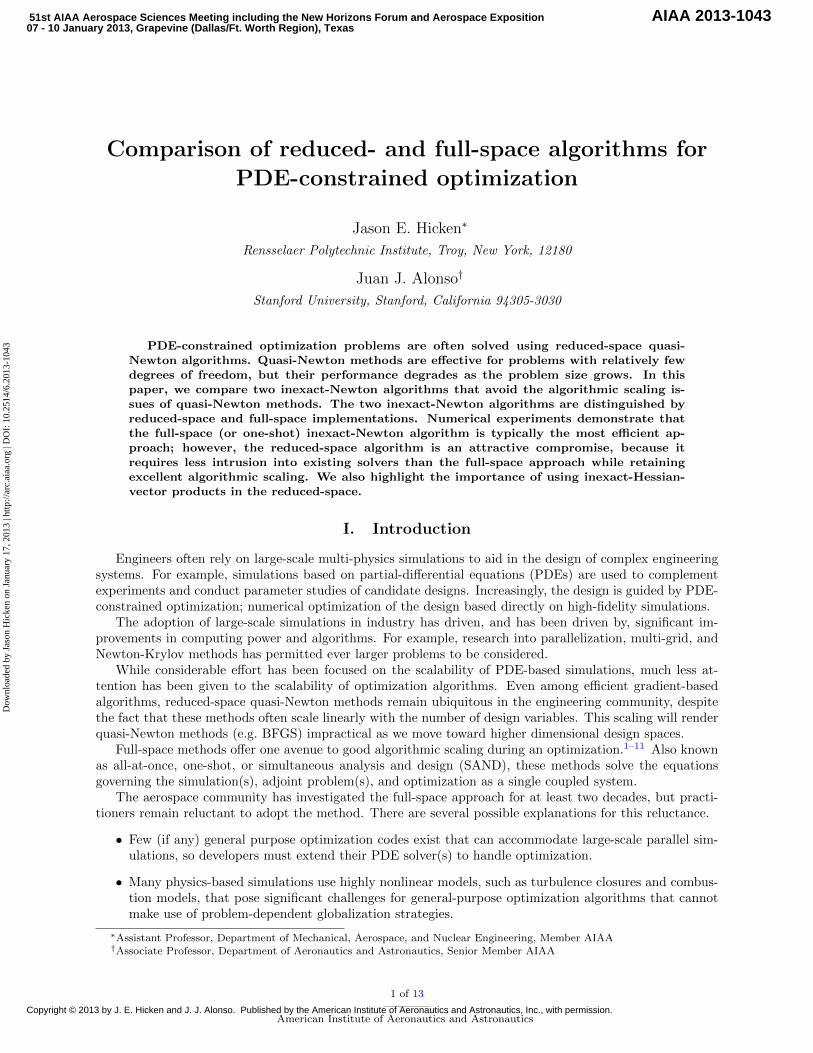
One of the advantages of the homotopy (7) over other parameter-continuation strategies is that theBFGS approximation can be reused when the parameter � changes. To see this, we recall the L-BFGSimplementation listed in Algorithm 1, which is based on a two-loop recursion.13 In the algorithm, Hk

denotes the quasi-Newton approximation to the Hessian and H0k is the initial approximate Hessian (taken

to be �I here). In the classical BFGS algorithm, sk � xk+1 � xk and zk = yk � gk+1 � gk. When usingthe parameter continuation described above, zk must be changed to be the di�erence between successivegradients of the modi�ed objective. At step k, the gradient of the modi�ed objective is (1��)gk+��(xk�x0);consequently, for a given � Algorithm 1 uses

zk � (1� �)(gk+1 � gk) + ��(xk+1 � xk)

= (1� �)yk + ��sk:

In practice we store si and yi for i = k� 1; k� 2; : : : ; k�m, as in the classical L-BFGS implementation, andrecompute zk on-the- y. This allows us to reuse gradient information from previous homotopy iterationsthat used di�erent � parameter values.

As is commonly done, the BFGS update is skipped if the curvature condition is violated; that is, ifsTk yk < 0. Notice that the curvature condition is computed using yk rather than zk, because as � ! 0 it isyk that we ultimately need to produce a positive-de�nite Hessian approximation. An alternative strategy,not pursued here, would be to keep yk until sTk zk < 0, and then discard this update. This could potentiallyaccelerate convergence in the early homotopy iterations.

Algorithm 1: Limited-memory BFGS with two-loop recursion

Data: uResult: v = H�1

k u

1 v = u2 for i = k � 1; k � 2; : : : ; k �m do3 �i 1

zTk sk

4 �i �isTi v

5 v v � �izi6 end

7 v �H0k

��1

v

8 for i = k �m; k �m+ 1; : : : ; k � 1 do9 �iz

Ti v

10 v v + (�i � )si11 end

4 of 13

American Institute of Aeronautics and Astronautics

Dow

nloa

ded

by J

ason

Hic

ken

on J

anua

ry 1

7, 2

013

| http

://ar

c.ai

aa.o

rg |

DO

I: 1

0.25

14/6

.201

3-10

43

III.C. Reduced-space inexact-Newton-Krylov Algorithm

As mentioned in the introduction, quasi-Newton methods can exhibit poor algorithmic scaling, and thismotivates methods that solve (6) more accurately. Let us reexamine this exact Newton update:

Hk�xk = �g(xk): (6)

If these update equations can be solved with su�cient accuracy, we may need signi�cantly fewer iterationsthan a quasi-Newton method. Ideally, we want a method that scales independently of the number of designvariables.

We can solve the linear system (6) with either a direct or iterative method. A direct method would requirethat we form, store, and factor the reduced Hessian at each iteration. Forming Hk explicitly requires thesolution of m linear systems of size n� n; therefore, we expect direct-solution methods to have algorithmiccomplexities similar to BFGS when applied to a quadratic objective.

Thus, we are left to consider iterative methods for (6). In particular, Krylov iterative methods areattractive, because they require products of Hk with arbitrary vectors w 2 Rm rather than the reducedHessian itself. Below, we will show that such Hessian-vector products can be computed e�ciently.

While Krylov subspace methods avoid the need to form Hk, they may require a signi�cant number ofiterations to converge. For example, assuming Hk is a symmetric-positive-de�nite matrix, the conjugategradient (CG) method requires m iterations to converge in exact arithmetic. This would again lead to analgorithmic complexity that is similar to BFGS.

Fortunately, we do not need to solve (6) exactly. In the early Newton iterations, the linear model istypically not an accurate representation of the gradient g(x). Therefore, it is unnecessary to solve for theroot of the linear model with high precision. This is the observation exploited by inexact-Newton methods,18

which are sometimes called truncated-Newton in the optimization literature.19 Rather than solve (6) exactly,an inexact-Newton reduced-space algorithm accepts approximate steps, pk 2 Rm, that satisfy the followinginequality.

kHkpk + g(xk)k � �kkg(xk)k; (8)

where �k 2 [0; 1) is the forcing parameter that controls the degree to which pk satis�es the Newton lineariza-tion. The subscript on �k indicates that the forcing parameter may change from one Newton-iteration tothe nextb. Most Krylov subspace solvers can easily accommodate the inexact-Newton condition (8).

The number of iterations needed by the Krylov solver can also be reduced through preconditioning;indeed, Krylov subspace methods must be preconditioned to be e�ective on most practical problems. Forthe present work, we maintain an L-BFGS quasi-Newton approximation to the Hessian and use this toprecondition the Krylov-subspace method.6,20

To �nd a step pk that satis�es (8), we employ the Flexible Generalized Minimal RESidual (FGMRES)method.12 The reduced Hessian is symmetric, which suggests using a Krylov iterative method with a short-term recurrence, e.g. MINRES;21 however, there are a couple important advantages to using FGMRES.

1. FGMRES permits the preconditioner to change from one Krylov iteration to the next; therefore, wecan dynamically update the L-BFGS approximation using the Hessian-vector product produced duringeach Krylov iteration. In contrast, non- exible Krylov methods can include the quasi-Newton updatesonly at the beginning of the next Newton iteration.20

2. More importantly, FGMRES explicitly orthogonalizes its basis vectors, which we have found is neces-sary when the Hessian-vector products are computed approximately; see Section III.C.1.

A disadvantage of using FGMRES is that 2 vectors of length m must be stored for each of its iterations. Forthe boundary-control problems typically encountered in aerodynamic shape optimization we have m � nand the additional storage is insigni�cant. For distributed control problems the additional storage maybecome an issue.

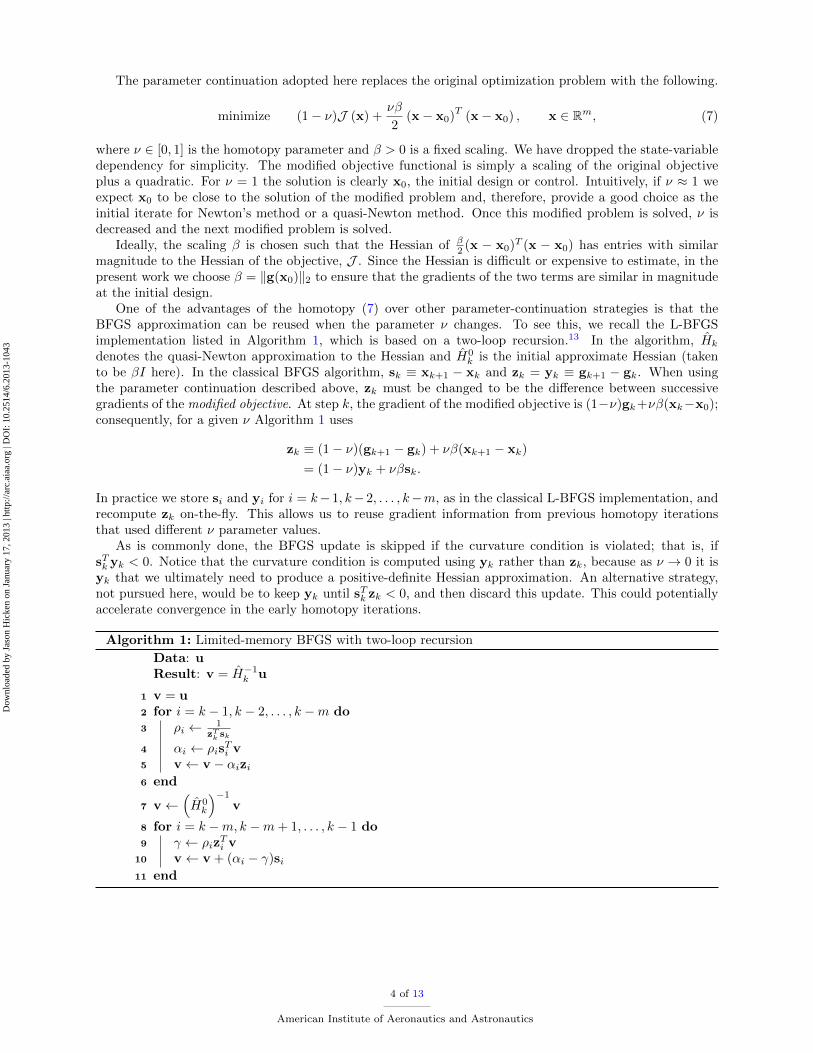
Algorithm 2 describes a generic reduced-space optimization using the homotopy-based globalizationmethod. The only signi�cant di�erence between the quasi-Newton version and the inexact-Newton-Krylov(INK) version is the computation of the step pk. At the end of each globalization loop, we use a simpleupdate for the continuation parameter; see line 18. The way that � is reduced can impact the e�ciency androbustness of the algorithm, and we do not claim that this particular update formula is appropriate for allcases.

bIn fact, �k must tend to zero su�ciently fast to recover quadratic convergence.

5 of 13

American Institute of Aeronautics and Astronautics

Dow

nloa

ded

by J

ason

Hic

ken

on J

anua

ry 1

7, 2

013

| http

://ar

c.ai

aa.o

rg |

DO

I: 1

0.25

14/6

.201

3-10

43

Algorithm 2: Generic reduced-space algorithm with homotopy-based globalization

Data: x0

Result: x satisfying g(x) = 0

1 x x0

2 for j = 0; 1; 2; : : : ; N do (globalization loop)3 for k = 0; 1; 2; : : : ; Nglobal do (Newton loop)4 solve R(x;u) = 0 for u (solve the primal problem)5 solve S(x;u; ) = 0 for (solve the adjoint problem)6 compute reduced gradient g(x;u; )7 compute modi�ed gradient: g� = (1� �)g + ��(x� x0)8 if kg�k2 � �global then (check convergence of modi�ed problem)9 exit Newton loop

10 end

11 solve Hkpk = �g� (quasi-Newton) or inexactly solve Hkpk = �g� (INK)12 x x + �pk (perform line search if using quasi-Newton)13 store si and yi (quasi-Newton update)

14 end15 if kgk2 � � then (check for convergence)16 exit globalization loop17 end18 � max (� � 0:1; 0)

19 end

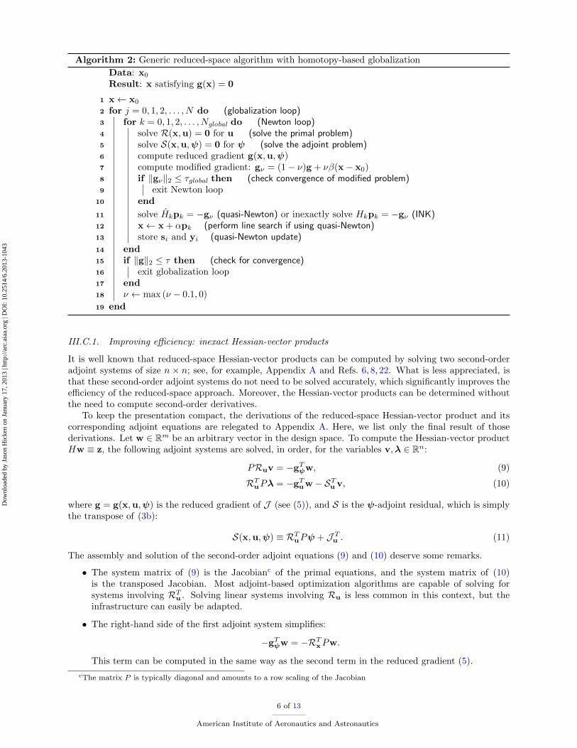
III.C.1. Improving e�ciency: inexact Hessian-vector products

It is well known that reduced-space Hessian-vector products can be computed by solving two second-orderadjoint systems of size n � n; see, for example, Appendix A and Refs. 6, 8, 22. What is less appreciated, isthat these second-order adjoint systems do not need to be solved accurately, which signi�cantly improves thee�ciency of the reduced-space approach. Moreover, the Hessian-vector products can be determined withoutthe need to compute second-order derivatives.

To keep the presentation compact, the derivations of the reduced-space Hessian-vector product and itscorresponding adjoint equations are relegated to Appendix A. Here, we list only the �nal result of thosederivations. Let w 2 Rm be an arbitrary vector in the design space. To compute the Hessian-vector productHw � z, the following adjoint systems are solved, in order, for the variables v;� 2 Rn:

PRuv = �gT w; (9)

RTuP� = �gTuw � STu v; (10)

where g = g(x;u; ) is the reduced gradient of J (see (5)), and S is the -adjoint residual, which is simplythe transpose of (3b):

S(x;u; ) � RTuP + J Tu : (11)

The assembly and solution of the second-order adjoint equations (9) and (10) deserve some remarks.

� The system matrix of (9) is the Jacobianc of the primal equations, and the system matrix of (10)is the transposed Jacobian. Most adjoint-based optimization algorithms are capable of solving forsystems involving RTu . Solving linear systems involving Ru is less common in this context, but theinfrastructure can easily be adapted.

� The right-hand side of the �rst adjoint system simpli�es:

�gT w = �RTxPw:

This term can be computed in the same way as the second term in the reduced gradient (5).

cThe matrix P is typically diagonal and amounts to a row scaling of the Jacobian

6 of 13

American Institute of Aeronautics and Astronautics

Dow

nloa

ded

by J

ason

Hic

ken

on J

anua

ry 1

7, 2

013

| http

://ar

c.ai

aa.o

rg |

DO

I: 1

0.25

14/6

.201

3-10

43

� The right-hand side vector of the adjoint system for � involves second derivatives; however, the potentialcomplications of computing second derivatives can be avoided by using a �nite-di�erence approxima-tion. Again, see Appendix A for the details.

Once v and � have been computed, the Hessian-vector product can be evaluated using the followingexpression:

Hw = gTx w + �TPRx(x;u) + vTPSx(x;u; ): (12)

As above, any second derivatives that appear can be approximated by using a �nite-di�erence approximation.The accuracy of the second-order adjoints v and � determines the accuracy of the Hessian-vector product

and, in large part, the computational expense of the entire INK algorithm. Thus, the tolerance we use tosolve the equations (9) and (10) plays an important role in the e�ciency of the algorithm and deservesfurther discussion.

If we use a short-term recurrence Krylov iterative method (e.g. CG, MINRES), then the Hessian-vectorproducts must be su�ciently accurate to maintain conjugacy/orthogonality between the Krylov subspacevectors. If conjugacy or orthogonality are lost due to inaccurate second-order adjoints, the linear systemmay fail to converge.23 This accuracy requirement imposed on the second-order adjoints leads to expensivereduced-space INK algorithms and is a frequently cited disadvantage of these methods.6,8

While the Hessian-vector product must be accurate for short-term recurrence methods, the productscan be computed inexactly if the Krylov iterative method maintains orthogonality of the solution subspaceexplicitly. This claim follows from theory of inexact-Krylov-subspace methods developed by Simoncini andSzyld.24 Indeed, their results indicate that, for methods like GMRES, the Hessian-vector products canbecome less accurate as the Krylov iterative method proceeds. As we shall see, the use of inexact-Hessianproducts is critical to the e�ciency of reduced-space INK methods.

IV. Full-space method

IV.A. Overview

In full-space methods, the nonlinear coupled system of equations (3) are solved simultaneously for thevariables (xTuT T ). For this reason, full-space methods are often referred to as one-shot, all-at-once, orsimultaneous-analysis-and-design methods.

Most full-space algorithms are based on some form of Newton’s method applied to (3). That is, ateach iteration k of the algorithm, the following linearized system is solved, or solved approximately, for theupdates � k+1 � k+1 � k, �uk+1 � uk+1 � uk, and �xk+1 � xk+1 � xk.264L ; L ;u L ;x

Lu; Lu;u Lu;x

Lx; Lx;u Lx;x

3750B@� k+1

�uk+1

�xk+1

1CA = �

264L Lu

Lx

375 : (13)

Newton’s method remains attractive here, because, under suitable conditions, it exhibits quadratic conver-gence. However, as usual, Newton’s method poses two challenges: the e�cient solution of the linear system(13) and globalization. Below, we will describe a full-space algorithm that addresses these issues.

IV.B. Full-space Inexact-Newton Algorithm

In this work we use a full-space algorithm that is based on the Lagrange-Newton-Krylov-Schur (LNKS)method of Biros and Ghattas.6,7 We brie y summarize our implementation below.

� We use the same homotopy-based globalization strategy adopted for the reduced-space algorithms, i.e.the term ��

2 (x� x0)T (x� x0) is added to the objective function, and � is gradually reduced to zero.

� A Krylov iterative method (e.g. FGMRES) is used to solve the Newton-update equation (13). Thefull-space Hessian-vector products are computed using a forward-di�erence approximation.

� We adopt the preconditioner ~P2 from Ref. 6, which was found to be the most e�cient in terms of CPUtime. This preconditioner approximates the full-space Hessian by dropping second-order terms, with

7 of 13

American Institute of Aeronautics and Astronautics

Dow

nloa

ded

by J

ason

Hic

ken

on J

anua

ry 1

7, 2

013

| http

://ar

c.ai

aa.o

rg |

DO

I: 1

0.25

14/6

.201

3-10

43

the exception of Lx;x, which is replaced with a L-BFGS quasi-Newton approximation. In addition, theJacobian Ru is replaced with a suitable preconditioner. Thus,

~P2 =

264 0 A PRx

AT 0 0

RTxP 0 H

375 ;where A and AT denote preconditioners for the linearized primal and dual PDEs, respectively. Notethat the global preconditioner has full rank; by assumption, A and AT are invertible, as is H.

V. Results

V.A. Steady quasi-one-dimensional nozzle ow

Our �rst comparison of the three optimization algorithms uses the inverse design of an inviscid nozzle. The ow is modelled using the quasi-one-dimensional Euler equations. For a spatially varying nozzle area, A(x),the governing equations are

@F@x� G = 0; 8 x 2 [0; 1]; (14)

where the ux and source are given by

F =

0B@ �uA

(�u2 + p)A

u(e+ p)A

1CA ; and G =

0B@ 0

pdAdx0

1CA ;

respectively. The unknown variables are the density, �, momentum per unit volume, �u, energy per unitvolume, e, and pressure, p. The underdetermined system is closed using the ideal gas law equation of statefor the pressure: p = ( � 1)(e� 1

2�u2).

Boundary conditions at the inlet and outlet are provided by the exact solution, which is determinedusing the Mach relations. The stagnation temperature and pressure are 300K and 100 kPa, respectively.The speci�c gas constant is taken to be 287 J/(kg K) and the critical nozzle area is A� = 0:8. The equationsand variables are nondimensionalized using the density and sound speed at the inlet.

The governing equations (14) are discretized using a third-order accurate diagonal-norm summation-by-parts scheme,25,26 with boundary conditions imposed weakly using penalty terms.27,28 Scalar third-orderaccurate arti�cial dissipation is added to prevent oscillatory solutions.29 The discretized Euler equations aresolved using a Newton-GMRES algorithm.30,31 GMRES32 is preconditioned using an LU factorization of a�rst-order accurate discretization based on nearest-neighbours. The linear adjoint problems are also solvedusing GMRES with the appropriate LU or UTLT factorized �rst-order preconditioner.

The nozzle area is parameterized using a cubic b-spline with an open uniform knot vector. The controlpoints at the ends of the nozzle are �xed such that the area satis�es A(0) = 2 and A(1) = 1:5. The designvariables are the remaining B-spline control points. The initial design x0 sets the control points to recovera nozzle with a linearly varying area between the �xed inlet and outlet. Figure 1(a) shows the initial nozzlearea and Mach number distribution. The target nozzle area is a cubic function of x that passes through theinlet and outlet areas and has a local minimum at x = 0:5 given by A(0:5) = 1; see Figure 1(b).

The objective function corresponds to an inverse problem for the pressure:

J =

Z 1

0

1

2(p� ptarg)2 dx: (15)

The objective function is discretized using a quadrature based on the SBP norm.33 The functional is fourth-order accurate, because the discretization is third-order accurate and adjoint consistent.34{36 The targetpressure ptarg is found by solving the discretized equations with the nozzle area speci�ed by the target area.

The optimal nozzle area produced by all three algorithms is indistinguishable from the target nozzle area,shown in Figure 1(b) together with the corresponding Mach number variation.

8 of 13

American Institute of Aeronautics and Astronautics

Dow

nloa

ded

by J

ason

Hic

ken

on J

anua

ry 1

7, 2

013

| http

://ar

c.ai

aa.o

rg |

DO

I: 1

0.25

14/6

.201

3-10

43

x

Mach

area

0.0 0.2 0.4 0.6 0.8 1.00.00

0.10

0.20

0.30

0.40

0.50

0.60

0.70

0.80

0.4

0.6

0.8

1.0

1.2

1.4

1.6

1.8

2.0

area

Mach

(a) initial

x

Mach

area

0.0 0.2 0.4 0.6 0.8 1.00.00

0.10

0.20

0.30

0.40

0.50

0.60

0.70

0.80

0.4

0.6

0.8

1.0

1.2

1.4

1.6

1.8

2.0

area

Mach

(b) optimized

Figure 1. Nozzle area and corresponding Mach number for the initial design (left) and optimized design (right).

cost (equivalent flow solutions)

no

rma

lize

d d

es

ign

gra

die

nt

50 100 150 200 250 300

10­3

10­2

10­1

100

LNKS

INK

QN

Figure 2. Convergence history of the normalized (design) gradient norm for the nozzle optimization problem with 60design variables.

The optimization algorithms begin with � = 0:5. The value of � is �xed until the reduced-gradient normof the modi�ed problem is less than 10% of its initial value (i.e. �global = 0:1). The continuation parameter isthen decreased by 0:1, and the process repeats until there is a three-order drop in the reduced-gradient normof the original problem (i.e. � = 103). In the case of the full-space algorithm, the primal and dual residualnorms must be reduced below 10�6 for convergence of the target problem. Both the full- and reduced-spaceINK algorithms use constant forcing parameters of �k = 0:1 in the Krylov solvers. The second-order adjointproblems for the reduced-Hessian-vector products are solved to a tolerance of 0:09 < �k.

Figure 2 compares the convergence histories of the reduced-gradient norm for the three optimizationalgorithms. The results shown are for 60 design variables, and computation cost is measured in terms ofequivalent ow solutions; more precisely, the cost is the number of preconditioner calls (both primal anddual) made by the optimization algorithm divided by the number of preconditioner calls made by a single ow solution.

The LNKS and INK algorithms exhibit rapid convergence typical of inexact-Newton schemes, and bothare signi�cantly faster than the quasi-Newton method. In particular, LNKS is more than an order ofmagnitude faster than the quasi-Newton method for this problem, and the INK algorithm is approximately4 times faster.

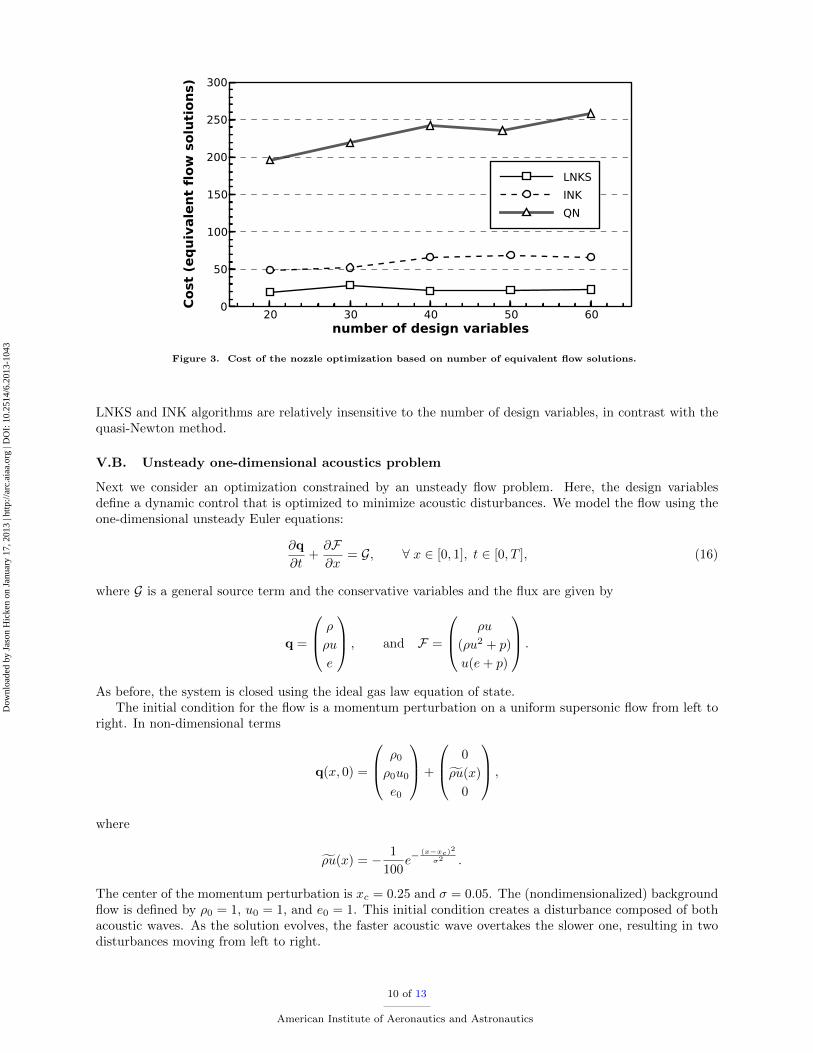
We are interested in how the algorithms scale as we increase the number of design variables. Figure 3plots the number of equivalent ow solutions required to converge the reduced-gradient norm 3 orders ofmagnitude, for design-space sizes between 20 and 60. Note that the quasi-Newton scheme failed for 50design variables, so the results reported are for 49 design variables. For the design spaces considered, the

9 of 13

American Institute of Aeronautics and Astronautics

Dow

nloa

ded

by J

ason

Hic

ken

on J

anua

ry 1

7, 2

013

| http

://ar

c.ai

aa.o

rg |

DO

I: 1

0.25

14/6

.201

3-10

43

20 30 40 50 60number of design variables

0

50

100

150

200

250

300

Cost

(eq

uiva

lent

flow

sol

utio

ns)

LNKSINKQN

Figure 3. Cost of the nozzle optimization based on number of equivalent ow solutions.

LNKS and INK algorithms are relatively insensitive to the number of design variables, in contrast with thequasi-Newton method.

V.B. Unsteady one-dimensional acoustics problem

Next we consider an optimization constrained by an unsteady ow problem. Here, the design variablesde�ne a dynamic control that is optimized to minimize acoustic disturbances. We model the ow using theone-dimensional unsteady Euler equations:

@q

@t+@F@x

= G; 8 x 2 [0; 1]; t 2 [0; T ]; (16)

where G is a general source term and the conservative variables and the ux are given by

q =

0B@ �

�u

e

1CA ; and F =

0B@ �u

(�u2 + p)

u(e+ p)

1CA :

As before, the system is closed using the ideal gas law equation of state.The initial condition for the ow is a momentum perturbation on a uniform supersonic ow from left to

right. In non-dimensional terms

q(x; 0) =

0B@ �0

�0u0

e0

1CA+

0B@ 0f�u(x)

0

1CA ;

where

f�u(x) = � 1

100e�

(x�xc)2

�2 :

The center of the momentum perturbation is xc = 0:25 and � = 0:05. The (nondimensionalized) background ow is de�ned by �0 = 1, u0 = 1, and e0 = 1. This initial condition creates a disturbance composed of bothacoustic waves. As the solution evolves, the faster acoustic wave overtakes the slower one, resulting in twodisturbances moving from left to right.

10 of 13

American Institute of Aeronautics and Astronautics

Dow

nloa

ded

by J

ason

Hic

ken

on J

anua

ry 1

7, 2

013

| http

://ar

c.ai

aa.o

rg |

DO

I: 1

0.25

14/6

.201

3-10

43

Table 1. Algorithm comparison for the unsteady problem.

nonlinear it. precond. calls equiv. ow

quasi-Newton 34 428 410 264.1

INK 3 85 780 52.9

LNKS 6 152 142 93.8

The objective function is the following space-time integral:

J =

Z T

0

Z 1

0

�(x)1

2(p� ptarg)2 dx dt;

where �(x) is a weighting kernel de�ned by

�(x) = e�(x�x�)2

�2 ;

with x� = 0:85. The target pressure is the unperturbed background pressure ptarg = p0 = 0:2.The Euler equations are discretized in space using a fourth-order accurate diagonal-norm SBP discretiza-

tion and 201 uniformly spaced nodes. The second-order accurate midpoint rule is used to advance thesolution in time. The nonlinear systems that arise at each iteration are solved using the same Newton-Krylov algorithm described in the preceding section. The time domain is divided into 200 intervals.

The control is a dynamic momentum source located at x = 0:5 and Gaussian in shape. The designvariables are the control’s magnitude at the midpoint of each time step; thus, as the time domain is re�nedthe design space is also re�ned. The source vector used in the midpoint rule for the time slab [Tk; Tk+1] isgiven by

GTk+ 12

=�

0 ske� (x�0:5)2

�2 0

�; (17)

where sk is the value of the kth design variable. Since there are 200 time steps, there are also 200 designvariables.

The results for this optimization problem are summarized in Table 1. The algorithms use the sameparameters as the previous example, except that no parameter continuation is necessary, so � = 0. Thereduced-gradient norm has been decreased by three orders of magnitude. As before, the INK and LNKSmethods are more e�cient than the quasi-Newton approach. Somewhat surprisingly, reduced-space INKrequires fewer equivalent ow solutions than LNKS on this problem.

VI. Conclusions

The algorithmic scaling of optimization algorithms must be considered if engineers are to tackle ever morecomplex designs using PDE-constrained optimization. Popular reduced-space quasi-Newton methods, whilerelatively easy to implement, scale poorly as the design-space dimension is increased. In contrast, full-spacemethods like LNKS o�er excellent scaling, but implementation challenges limit their broad acceptance.

To �nd a suitable compromise, we have developed a novel inexact-Newton-Krylov (INK) method for PDE-constrained optimization that is applied in the reduced space. A novel element of the INK method is the useof inexact-Hessian-vector products, which is critical to its e�ciency. Numerical experiments con�rm thatthe proposed INK method has good algorithmic scaling as the number of design variables grows. Moreover,the reduced-space INK algorithm is signi�cantly easier to implement than full-space one-shot methods.

A. Derivation of the reduced-space Hessian-vector product

Let w 2 Rm be a arbitrary vector in the design space and let g = g(x;u; ) be the reduced gradient ofJ ; see (5). We begin by recognizing that the inner product gTw is a functional whose total derivative is thedesired Hessian-vector product Hw � z. This functional depends on the design variables, the state variables,and the (�rst-order) adjoint variables. The state variables and adjoint variables are implicit functions of the

11 of 13

American Institute of Aeronautics and Astronautics

Dow

nloa

ded

by J

ason

Hic

ken

on J

anua

ry 1

7, 2

013

| http

://ar

c.ai

aa.o

rg |

DO

I: 1

0.25

14/6

.201

3-10

43

design variables through their respective governing equations, so the appropriate Lagrangian for computingthe total derivative of gTw is

L(x;u; ;v;�) � gTw + �TPR(x;u) + vTS(x;u; ):

We have introduced two additional adjoint variables: � for the primal residual R and v for the residual of(3b), denoted by S:

S � RTuP + J Tu : (11)

The desired Hessian-vector product is the derivative of L with respect to x:

Hw = Lx = gTx w + �TPRx(x;u) + vTSx(x;u; ): (12)

Note that the partial derivatives with respect to x treat u, , �, and v as constant. For example,

gx = @x

hJx + TPRx

i= Jxx + TPRxx:

While there are second derivatives in the expression for Hw, they always appear as products with othervectors. Thus, they can be approximated using �nite-di�erence approximations. To illustrate this, considerthe forward-di�erence approximation of gTx w, which is given by

gTx w =g(x + �w;u; )� g(x;u; )

�+ O(�);

where � > 0 is the perturbation parameter.The expression for Hw depends on v and �, so we need to solve for these adjoint variables. The linear

systems that determine v and � can be found by di�erentiating L with respect to and u, respectively.After di�erentiating and rearranging, we arrive at

PRuv = �gT w; (9)

RTuP� = �gTuw � STu v: (10)

As noted in the text, the right-hand-side of (9) reduces to �RTxPw, which can be computed in the same wayas the term TPRx that appears in the gradient. The right-hand-side of (10) contains second-derivatives,but as above, these can be approximated using �nite-di�erence approximations. For example,

STu v =S(x;u + �v; )� S(x;u; )

�+ O(�):

References

1Frank, P. D. and Shubin, G. R., \A comparison of optimization-based approaches for a model computational aerodynamicsdesign problem," Journal of Computational Physics, Vol. 98, No. 1, Jan. 1992, pp. 74{89.

2Ta’asan, S., Kuruvila, G., and Salas, M. D., \Aerodynamic design and optimization in one shot," The 30th AIAAAerospace Sciences Meeting and Exhibit , No. AIAA{1992{25, Jan. 1992.

3Iollo, A., Salas, M. D., and Ta’asan, S., \Shape optimization governed by the Euler equations using an adjoint method,"Tech. Rep. ICASE 93-78, NASA Langley Research Center, Hampton, Virginia, Nov. 1993.

4Feng, D. and Pulliam, T. H., \An all-at-once reduced Hessian SQP scheme for aerodynamic design optimization," Tech.Rep. RIACS-TR-95.19, NASA Ames Research Center, Mo�ett Field, California, Oct. 1995.

5Gatsis, J. and Zingg, D. W., \A fully-coupled Newton-Krylov algorithm for aerodynamic optimization," 16th AIAAComputational Fluid Dynamics Conference, No. AIAA{2003{3956, Orlando, Florida, United States, June 2003.

6Biros, G. and Ghattas, O., \Parallel Lagrange-Newton-Krylov-Schur methods for PDE-constrained optimization. Part I:the Krylov-Schur solver," SIAM Journal on Scienti�c Computing, Vol. 27, 2005, pp. 687{713.

7Biros, G. and Ghattas, O., \Parallel Lagrange-Newton-Krylov-Schur methods for PDE-constrained optimization. PartII: the Lagrange-Newton solver and its application to optimal control of steady viscous ows," SIAM Journal on Scienti�cComputing, Vol. 27, 2005, pp. 714{739.

8Haber, E. and Ascher, U. M., \Preconditioned all-at-once methods for large, sparse parameter estimation problems,"Inverse Problems, Vol. 17, No. 6, Nov. 2001, pp. 1847{1864.

9Hazra, S. B., \An e�cient method for aerodynamic shape optimization," 10th AIAA/ISSMO Multidisciplinary Analysisand Optimization Conference, No. AIAA{2004{4628, Albany, New York, Aug. 2004.

12 of 13

American Institute of Aeronautics and Astronautics

Dow

nloa

ded

by J

ason

Hic

ken

on J

anua

ry 1

7, 2

013

| http

://ar

c.ai

aa.o

rg |

DO

I: 1

0.25

14/6

.201

3-10

43

10Hazra, S. B., \Direct treatment of state constraints in aerodynamic shape optimization using simultaneous pseudo-time-stepping," AIAA Journal , Vol. 45, No. 8, Aug. 2007, pp. 1988{1997.

11Hazra, S. B., \Multigrid one-shot method for state constrained aerodynamic shape optimization," SIAM Journal onScienti�c Computing, Vol. 30, No. 6, 2008, pp. 3220{3248.

12Saad, Y., \A exible inner-outer preconditioned GMRES algorithm," SIAM Journal on Scienti�c and Statistical Com-puting, Vol. 14, No. 2, 1993, pp. 461{469.

13Nocedal, J. and Wright, S. J., Numerical Optimization, Springer{Verlag, Berlin, Germany, 2nd ed., 2006.14Pierce, N. A. and Giles, M. B., \An introduction to the adjoint approach to design," Flow, Turbulence and Combustion,

Vol. 65, No. 3, 2000, pp. 393{415.15Liu, D. C. and Nocedal, J., \On the limited memory BFGS method for large scale optimization," Mathematical Pro-

gramming, Vol. 45, 1989, pp. 503{528.16Fletcher, R., Practical methods of optimization, A Wiley-Interscience Publication, Wiley, 2nd ed., 2000.17Allgower, E. L. and Georg, K., Acta Numerica, chap. Continuation and Path Following, Cambridge University Press,

1993, pp. 1{64.18Dembo, R. S., Eisenstat, S. C., and Steihaug, T., \Inexact Newton methods," SIAM Journal on Numerical Analysis,

Vol. 19, No. 2, 1982, pp. 400{408.19Nash, S. G., \A survey of truncated-Newton methods," Journal of Computational and Applied Mathematics, Vol. 124,

No. 1-2, 2000, pp. 45{59.20Morales, J. L. and Nocedal, J., \Automatic Preconditioning by Limited Memory Quasi-Newton Updating," SIAM Journal

on Optimization, Vol. 10, No. 4, 2000, pp. 1079{1096.21Paige, C. C. and Saunders, M. A., \Solution of Sparse Inde�nite Systems of Linear Equations," SIAM Journal on

Numerical Analysis, Vol. 12, No. 4, 1975, pp. 617{629.22Hinze, M. and Pinnau, R., \Second-order approach to optimal semiconductor design," Journal of Optimization Theory

and Applications, Vol. 133, 2007, pp. 179{199.23Golub, G. H. and Ye, Q., \Inexact Preconditioned Conjugate Gradient Method with Inner-Outer Iteration," SIAM

Journal on Scienti�c Computing, Vol. 21, No. 4, 1999, pp. 1305{1320.24Simoncini, V. and Szyld, D. B., \Theory of Inexact Krylov Subspace Methods and Applications to Scienti�c Computing,"

SIAM Journal on Scienti�c Computing, Vol. 25, No. 2, Jan. 2003, pp. 454{477.25Kreiss, H. O. and Scherer, G., \Finite element and �nite di�erence methods for hyperbolic partial di�erential equations,"

Mathematical Aspects of Finite Elements in Partial Di�erential Equations, edited by C. de Boor, Mathematics Research Center,the University of Wisconsin, Academic Press, 1974.

26Strand, B., \Summation by parts for �nite di�erence approximations for d/dx," Journal of Computational Physics,Vol. 110, No. 1, 1994, pp. 47{67.

27Funaro, D. and Gottlieb, D., \A new method of imposing boundary conditions in pseudospectral approximations ofhyperbolic equations," Mathematics of Computation, Vol. 51, No. 184, Oct. 1988, pp. 599{613.

28Carpenter, M. H., Gottlieb, D., and Abarbanel, S., \Time-stable boundary conditions for �nite-di�erence schemes solvinghyperbolic systems: methodology and application to high-order compact schemes," Journal of Computational Physics, Vol. 111,No. 2, 1994, pp. 220{236.

29Mattsson, K., Sv�ard, M., and Nordstr�om, J., \Stable and accurate arti�cial dissipation," Journal of Scienti�c Computing,Vol. 21, No. 1, 2004, pp. 57{79.

30Keyes, D. E., \Aerodynamic applications of Newton-Krylov-Schwarz solvers," Proceedings of the 14th InternationalConference on Numerical Methods in Fluid Dynamics, Springer, New York, 1995, pp. 1{20.

31Nielsen, E. J., Walters, R. W., Anderson, W. K., and Keyes, D. E., \Application of Newton-Krylov methodology to athree-dimensional unstructured Euler code," 12th AIAA Computational Fluid Dynamics Conference, San Diego, CA, 1995.

32Saad, Y. and Schultz, M. H., \GMRES: a generalized minimal residual algorithm for solving nonsymmetric linear sys-tems," SIAM Journal on Scienti�c and Statistical Computing, Vol. 7, No. 3, July 1986, pp. 856{869.

33Hicken, J. E. and Zingg, D. W., \Summation-by-parts operators and high-order quadrature," Journal of Computationaland Applied Mathematics, Vol. 237, No. 1, Jan. 2013, pp. 111{125.

34Lu, J. C., An a posteriori error control framework for adaptive precision optimization using discontinuous Galerkin �niteelement method , Ph.D. thesis, Massachusetts Institute of Technology, Cambridge, Massachusetts, 2005.

35Hartmann, R., \Adjoint Consistency Analysis of Discontinuous Galerkin Discretizations," SIAM Journal on NumericalAnalysis, Vol. 45, No. 6, 2007, pp. 2671{2696.

36Hicken, J. E. and Zingg, D. W., \The role of dual consistency in functional accuracy: error estimation and superconver-gence," 20th AIAA Computational Fluid Dynamics Conference, No. AIAA-2011-3855, Honolulu, Hawaii, United States, June2011.

13 of 13

American Institute of Aeronautics and Astronautics

Dow

nloa

ded

by J

ason

Hic

ken

on J

anua

ry 1

7, 2

013

| http

://ar

c.ai

aa.o

rg |

DO

I: 1

0.25

14/6

.201

3-10

43