CFD modelling of a Diesel engine combustion using Ansys Fluent ...

Comparison of Reaction in Catalyst Pellet Between Three-Dimensional Computational Fluid Dynamics and
One-Dimensional Multiphysics Simulations
A Major Qualifying Project Report Submitted to the Faculty of Worcester Polytechnic Institute in partial fulfillment of the requirements for the
Degree of Bachelor of Science
Submitted by:
________________________________ Christian P. Waller
April 2010
Approved by: _____________________________ Dr. Anthony G. Dixon, Advisor

i
EXECUTIVE SUMMARY
The field of computational fluid dynamics (CFD) was developed with the advent of powerful
computing hardware in the mid-twentieth century. Computational fluid dynamics revolutionized research
into fluid dynamics because of its ability to numerically solve difficult systems of equations. As
commercially available CFD code evolved the number of industries which found use for such an
application also grew. Recently the field of chemical reaction engineering has applied CFD to the difficult
problems of characterizing heat, mass transfer, and fluid flow effects on chemical systems.
This study investigates the kinetics of the esterification of methanol and acetic acid into methyl
acetate and water so that this reaction can be simulated using CFD. Fluent, a popular CFD package, was
used to simulate the esterification reaction in a β-zeolite catalyst pellet using a three-dimensional (3D)
model. The reaction and diffusion limitations of the system are characterized by examining the effects of
various aspects of the pellet geometry, such as edges and holes. The distribution of products throughout
the pellet is shown to qualitatively agree with data obtained from H-NMR analysis with a fair degree of
accuracy.
Due to a lack of experimental data to validate the model, this study focuses instead on
approximating the complex 3D geometry by a simpler 1D system modeled in the multiphysics software
COMSOL. In particular, the relationship between catalyst surface area, catalyst volume, and overall
reaction rate is examined. The results of the 3D and 1D simulations demonstrate that a properly defined
1D system can accurately model some aspects of a 3D system – for example, the internal concentration
profile was approximated by the 1D model very well, but the overall reaction rate was significantly
different from that given by the 3D model. Several suggestions are made on how this project can be
expanded and improved upon in the future.

ii
ACKNOWLEDGEMENTS
The work presented in the report is the direct result of the contributions of several individuals
who helped guide me throughout this process. Without the influence and mentoring of these people I
would not have been able to accomplish as much as I have.
First and foremost I would like to extend my sincere gratitude to Professor A. G. Dixon for his
continual academic and moral support throughout the entirety of this process. Professor Dixon’s
experience with conducting academic research and expertise in the field of computational fluid dynamics
have both proved to be invaluable resources.
I also owe a great deal of gratitude to the members of the steam reforming group at the Chilton
site of Johnson Matthey in Billingham, UK. Specifically I would like to acknowledge Dr. Michiel
Nijemeisland and Dr. E. Hugh. Stitt. The guidance which I was lucky enough to receive during my first
foray into the world of industrial chemical engineering opened my eyes to the opportunities which await
me after graduation. Both Dr. Nijemisland and Dr. Stitt served as excellent role models and examples of
true professionals. Thank you for making this project possible.
iii
TABLE OF CONTENTS
Executive Summary ....................................................................................................................................... i
Acknowledgements ....................................................................................................................................... ii
1. Introduction ............................................................................................................................................... 1
1.1. Problem Statement ............................................................................................................................. 2
2. Background ............................................................................................................................................... 4
2.1. Cation Exchange Polymers ................................................................................................................ 4
2.2. Heterogeneous Catalysis .................................................................................................................... 5
2.2.1. Steps in a Heterogeneous Catalytic Reaction .............................................................................. 6
2.2.2. Importance of External Diffusion in Heterogeneous Reactions .................................................. 7
2.3. Esterification Reaction Mechanism and Rate Models ....................................................................... 8
2.3.1. Mechanism of Esterification of Acetic Acid and Methanol ........................................................ 8
2.3.2. Pseudo-Homogeneous ................................................................................................................. 9
2.3.3. Water Inhibition on Cation Exchange Polymers ....................................................................... 10
2.4. Historical Methods of Investigating Diffusion and Reaction in Heterogeneous Catalysis .............. 10
2.4.1. Homogeneous Models............................................................................................................... 11
2.4.2. Heterogeneous Models .............................................................................................................. 12
2.5. Computational Fluid Dynamics ....................................................................................................... 15
2.5.1. CFD Problem Analysis ............................................................................................................. 15
2.5.2. Theory of CFD .......................................................................................................................... 17
2.5.3. Spatial Discretization Methods ................................................................................................. 18
2.5.4. Numerical Solutions .................................................................................................................. 20
2.5.5. Application of CFD to Chemical Reaction Engineering ........................................................... 21
3. Kinetic Experiments ................................................................................................................................ 24
3.1. Goals ................................................................................................................................................ 24
3.2. Methodology .................................................................................................................................... 24
3.3. Results .............................................................................................................................................. 26
3.4. Discussion ........................................................................................................................................ 27
4. Methodology ........................................................................................................................................... 32
4.1 System Design .................................................................................................................................. 32

iv
4.1.1. Generating the System Geometry ............................................................................................. 32
4.1.2. Generating the System Mesh .................................................................................................... 33
4.1.3. Specifying the Geometry Boundary and Continuum Conditions .............................................. 34
4.2. Computational Fluid Dynamics Modeling ....................................................................................... 34
4.2.1. Use of User Defined Scalars ..................................................................................................... 35
4.2.2. System Definitions .................................................................................................................... 35
4.2.3 Simulation Solving ..................................................................................................................... 38
4.3. Multiphysics Modeling .................................................................................................................... 38
4.3.1. System Geometry and Mesh ..................................................................................................... 38
4.3.2. System Definitions .................................................................................................................... 39
5. Results ..................................................................................................................................................... 41
5.1. 3D CFD Model ................................................................................................................................ 41
5.1.1. CFD Model Verification ........................................................................................................... 41
5.1.2. Overall Reaction and Molar Flow Rates ................................................................................... 42
5.1.3. Characterization of Pellet Surface ............................................................................................. 43
5.1.4. Characterization of Pellet Internals ........................................................................................... 44
5.1.5. Qualitative Validation of CFD Model ...................................................................................... 47
5.2. 1D Multiphysics Model ................................................................................................................... 48
5.2.1. 1D Model Verification .............................................................................................................. 48
5.2.2. Overall Reaction Rates .............................................................................................................. 49
5.2.3. Comparison to 3D Simulation ................................................................................................... 50
6. Conclusions and Recommendations ....................................................................................................... 53
Nomenclature .............................................................................................................................................. 55
References ................................................................................................................................................... 57
APPENDIX A: Gas-Liquid Chromatography Data Conversion ................................................................. 59
APPENDIX B: Sample Gambit Journal ..................................................................................................... 64
APPENDIX C: 3D Simulation Convergence Plots ..................................................................................... 68

1
CHAPTER 1
Introduction
The chemical process industry, which employs more than one million individuals and generates
more than $400 billion per annum in the United States alone, produces the materials which make nearly
every commercially available product. Catalysts play an integral role in this industry by facilitating a wide
range of chemical processes including steam reforming, ammonia synthesis, methanol synthesis,
hydrocracking, and hydrodealkylation. Over 70% of industrial processes utilize catalysts, accounting for
over 90% by volume of chemical products (Catalytic Processes and Materials, 2011). Proper catalyst
design requires one to consider a wide range of design variables, such as particle geometry, size, and
diffusion characteristics (Sie & Kirshna, 1998). A thorough understanding of the mechanisms of transport
and reaction within catalysts allows for improvements upon the design of existing catalysts, thereby
increasing the economic incentive of processes.
The foundations of modern research into the diffusion and reaction phenomena of catalysis were
laid in the seventeenth century with the birth of experimental fluid dynamics. Early experiments provided
empirical data on fluid flow, such as the relationship between drag and the square of velocity. Towards
the end of the seventeenth century the theoretical framework of fluid dynamics began to take form,
beginning with the theoretical derivation of the velocity-squared law from the laws presented in Newton’s
Principia. Advancements in the realm of theoretical fluid dynamics continued throughout the eighteenth
and nineteenth centuries via the research of Bernoulli, Pitot, Euler, Navier, Stokes, and others.
Research in all fields of engineering and science existed in two worlds, pure theory and pure
experiment, until the advent of computers in the 1960s. The raw computational power of computers
coupled with numerical algorithms which describe fluid flow, diffusion, and reaction provided researchers
with a tool to numerically solve systems of equations which would be difficult or impossible to solve

2
otherwise. Additionally, the ability to numerically simulate fluid dynamics and reaction allowed scientists
to investigate phenomena in locations which are inaccessible in the laboratory due to limitations in
experimentation technology. For example in systems which operate at a high temperature or pressure (e.g.
steam methane reforming) or are highly corrosive the extreme conditions preclude gathering data via
physical experimentation, thereby rendering simulation as the only method of data acquisition.
As computing technology matured and more powerful processors were developed, increasingly
complex simulations could be solved. While early simulations of diffusion and reaction investigated
catalysis in one particle in one dimension (1D), modern simulations often model tens, if not hundreds, of
particles in three dimensions (Nijemeisland & Dixon, 2001). The advantages offered by 3D simulations
over 1D simulations (namely a closer approximation of reality) are counterbalanced by the drawbacks
introduced by the dramatic increase in the complexity of the system – namely an increase in the time and
computational power needed to solve the simulation. Because any given chemical process can operate
under a range of conditions, simulating every set of operating conditions requires a significant investment
of time and capital. Therefore, it is desirable to reduce a complex 3D model to a simpler 1D or 2D model
whenever it is possible to do so without sacrificing the quality of the simulation results.
1.1. Problem Statement The present study investigates diffusion and reaction within a 3D catalyst pellet. compares
diffusion and reaction in 3D computational fluid dynamics simulations to diffusion and reaction in 1D
multiphysics simulations. The reaction of interest is the forward reaction of the esterification of methanol
and acetic acid into methyl acetate and water over a β-zeolite catalyst (the reverse reaction and
dimerization reaction of methyl acetate into dimethyl acetate are not considered), which is given by:
CH3OH + CH3COOH β−zeolite�⎯⎯⎯⎯⎯� CH3COOCH3 + H2
The original intent of the work was to compare the results of 3D CFD simulations to experimental
H-NMR data of reaction over a catalyst pellet. Magnetic resonance imaging (specifically H-NMR
imaging) has been recognized as a powerful tool to noninvasively investigate diffusion and reaction inside

3
of a catalyst particle in situ (Huang, Yijiao, Reddy Marthala, Wang, Sulikowski, & Hunger, 2007).
Unfortunately the H-NMR experiments failed to produce any quantitative results due to a lack of
chemical resolution for the chosen system – the only data of significance shows a qualitative distribution
of methanol within the pellet. Therefore the focus of the project shifted to comparing the results of
diffusion and reaction in 3D computational fluid dynamics simulations to 1D multiphysics simulations in
order to determine whether a 1D approximation of a 3D geometry can provide accurate results.
The 3D system geometry was generated using GAMBIT 2.4.6, a computer aided design program.
The CFD simulations were completed in Fluent 6.3.26 in 3D using the finite volume spatial discretization
method. The multiphysics simulations were completed in COMSOL 3.5a using the Mass Transport
application in the Chemical Engineering Module in 1D using a finite element scheme.
Both the 1D and 3D simulations required information about the kinetics and diffusion of the
system. In order to supply the former, a kinetic experiment was designed and carried out to determine the
temperature dependence of the rate constant of the reaction. The diffusion parameters for species
transport were calculated using the Wilke-Chang equation.

4
CHAPTER 2
Background
2.1. Cation Exchange Polymers Solid catalysts are widely used in the chemical process industry to facilitate a number of chemical
processes (e.g. steam reforming, ammonia synthesis, alcohol synthesis). One reason heterogeneous
catalysts are widely used is that they offer several economic advantages compared to their homogeneous
counterparts. Some of these advantages include ease of product separation from catalyst material, less
potential for contamination, and reduced potential for equipment corrosion (Harmer & Sun, 2001).
Cation exchange polymers are one class of heterogeneous catalysts. Ion exchange polymers are
insoluble in and can exchange ions (existing within its pores) with a fluid passing through it. One
category of cation exchange catalysts are known as zeolites. Zeolites are crystalline aluminosilicates
whose three-dimensional structures boast the unique property of uniform pore sizes (Maesen, 2007, p. 1).
The crystal structure of zeolites (see Figure 1) consists primarily of SiO2, but at certain sites the silicon
has been replaced by aluminum. A charge imbalance is introduced at sites
where Al3+ replaces Si4+ and gives the crystal a net negative charge which
allows various cations (e.g. Na+, K+, Ca2+ etc.) to enter its pores.
Zeolites, whose pores measure on the molecular scale, are
commonly used as molecular sieves which selectively allow diffusion of
molecules which are small enough to fit inside its pores. This property of
zeolites makes them an attractive option when a high degree of
selectivity is required, as in the case for the formation of xylene from
toluene and methane (Fogler, 2006). In this reaction methane and toluene diffuse into the zeolite and react
FIGURE 1: B-ZEOLITE CRYSTAL STRUCTURE

5
to form a mixture of ortho, meta, and para xylenes. Due to the size of the pores only para-xylene is able to
diffuse out of the zeolite, while ortho- and meta-xylene react on interior active sites to isomerize into
para-xylene. Although molecules are constantly diffusing into and out of the zeolite, the crystal typically
retains its original structure with no appreciable changes in size or conformation (Dyer, 2007, p. 532).
The catalyst used in this study was β-zeolite, a large-pored zeolite which is used in processes such
as catalytic cracking, isomerization, alkylation, and disproportionation (Su & Norberg, 1997). This
catalyst is a solid acid catalyst which offers the functionality of an acid to facilitate the esterification
reaction on a solid matrix, allowing for easy separation of products from the catalyst.
2.2. Heterogeneous Catalysis Heterogeneous catalysis typically occurs at the interface between two or more phases. For the
esterification reaction considered in this study, the fluid mixture consisting primarily of methanol and
ethanol constitutes the first phase and the zeolite catalyst is the second phase. Because the catalytic
reaction occurs at the interface between phases, catalysts are typically designed to maximize surface area
without compromising necessary mechanical properties of the catalyst structure. The most common
method of maximizing the surface of a catalyst is to introduce an internal porous structure. Typical silica-
alumina cracking catalysts have pore volumes of 0.6 cm3/g and pore radii of 4 nm, resulting in surface
areas of 300 m2/g (Fogler, 2006).
In contrast to porous catalysts where the active material is part of the support structure, supported
catalysts have the active material dispersed over the surface of a less active substrate which provides the
catalyst structure. Supported catalysts are an attractive option when the active material is very expensive,
as is the case with pure metals or metal alloys. A third category of catalysts is monolithic catalysts. These
catalysts offer such high activity that they do not require a porous structure to achieve high reaction rates.
These catalysts are typically used in reactions where pressure drop and heat removal are major concerns,
such as the catalytic conversion of combustion engine exhaust gases (Fogler, 2006).

6
2.2.1. Steps in a Heterogeneous Catalytic Reaction The first step in a heterogeneous catalytic reaction involves mass transfer from the bulk fluid to
the external catalyst surface. In order to reach the catalyst surface, reactants must diffuse through a
boundary layer which surrounds the catalyst pellet. The rate of mass transfer for a reactant A at bulk
concentration CAb diffusing through a mass transfer boundary layer is given by
Rate = kc(CAb − CAs)
where kc is the mass transfer coefficient which accounts for the resistance to mass transfer resulting from
the boundary layer and CAs is the concentration of A at the external catalyst surface. Further discussion of
the mass transfer coefficient and effects of external diffusion follow in Section 2.2.2.
After reaching the external surface of the catalyst, reactant A must diffuse from the external
surface through the pore network of the pellet. While diffusing through the pore network, reactant A
encounters active catalyst sites along the pellet walls and reacts. Whether or not internal diffusion limits
the overall rate of reaction is dependent upon pellet size (Fogler, 2006). In a large pellet it takes a long
time for species to diffuse into and out of the pellet interior, thus reaction is limited to areas near the
external surface of the pellet. For a small pellet, species readily diffuse into and out of the pellet and
reaction occurs throughout the entire pore network.
When the reactant A encounters an active catalyst site, it must be adsorbed onto the catalyst
surface. This process is represented by the reaction. The rate of adsorption of species A onto active sites is
directly proportional to the concentration of A and the concentration of vacant sites. The rate at which A
desorbs from active sites without reacting is generally a first order process which is directly proportional
to the concentration of active sites occupied by A (Fogler, 2006). The rate of adsorption is nearly
independent of temperature while the rate of desorption increases exponentially with increasing
temperature (Fogler, 2006).
Once reactant A is adsorbed onto the active site the reaction can proceed in a number of different
ways, such as via the Eley-Rideal reaction. Following reaction, the products must leave the active sites
via desorption.

7
Both the transport (i.e. diffusion, adsorption, and desorption) steps and reaction steps contribute
to the overall reaction rate of the system. If the diffusion steps are much slower than the reaction steps,
the system is said to be diffusion limited. In such a system the reactant species are converted to products
faster than new reactant species can diffuse to the active sites of the catalyst. In contrast, if the reaction
occurs much slower than the diffusion of species from the bulk fluid to the external catalyst surface, the
system is said to be reaction limited. Because the diffusion of molecules occurs much quicker than the
reaction, the concentration of species in the bulk fluid and at active sites within the catalyst is constant
(Fogler, 2006).
2.2.2. Importance of External Diffusion in Heterogeneous Reactions External diffusion can play a major role in the overall reaction rate of a heterogeneous catalytic
reaction. When a species diffuses into a catalyst pellet, it must pass through a mass transfer boundary
layer which surrounds the catalyst pellet. The thickness of this boundary layer is defined as the distance
from the surface of the solid to the point where the concentration of the diffusing species equals 99% of
its bulk concentration (Fogler, 2006). This boundary decreases in thickness with increasing velocity.
Therefore, because the mass transfer boundary layer effectively accounts for all of the resistance to mass
transfer from the bulk fluid to the pellet, external diffusion can be neglected at high fluid velocities.
The simplest definition of the mass transfer coefficient is
kc =Dfluid
∂
where Dfluid is the diffusivity of the fluid and ∂ is the thickness of the mass transfer boundary layer.
However, it is difficult to experimentally determine the thickness of the boundary layer surrounding the
pellet. Fortunately there exist a number of heat transfer correlations which are analogous to mass transfer
correlations. As the one-dimensional simulation presented in this study used a spherical pellet model, the
Frössling correlation (Equation 2) for flow around a single sphere is most appropriate.
Sh = 2 + 0.6Re1/2Sc1/3
EQUATION 1
EQUATION 2

8
The Sherwood (Sh), Reynolds (Re), and Schmidt (Sc) numbers are given by
Sh =kcdpDfluid
Re =ρdvµ
Sc =µ
ρDfluid
where dp is the particle diameter, ρ is the fluid density, v is the fluid velocity, and µ is the dynamic
viscosity of the fluid. The Frössling correlation shows that in order to increase the mass transfer
coefficient one must either decrease the particle size or increase the fluid velocity.
2.3. Esterification Reaction Mechanism and Rate Models
2.3.1. Mechanism of Esterification of Acetic Acid and Methanol The reaction of esterification of acetic acid and methanol is a well-studied reaction. The
mechanism for this reaction over a solid acid catalyst proceeds by the following steps (Teo & Saha,
2004). In the first step a hydrogen atom from the acid catalyst protonates the acetic acid.
This protonation forms an unstable transition state which is stabilized when a pair of electrons leaves the
π bond between carbon and oxygen and becomes a lone pair on the oxygen. This movement of electrons
forms a primary carbocation which is then attacked by the nucleophile methanol.
EQUATION 3
EQUATION 4
EQUATION 5

9
An unstable oxygen cation is formed once again, and the molecule quickly transfers hydrogen atom from
the oxygen cation to a nearby oxygen where there is a region of greater electron density. The transfer of
off of the oxygen cation creates a good leaving group and the molecule loses a molecule of water,
creating a primary carbocation. To stabilize the molecule, the oxygen atom which is not bonded to the
methyl group simultaneously donates a pair of electrons to form a π bond with the carbon atom.
In the final step of the reaction the water molecule deprotonates the oxygen cation, resulting in the
product methyl ester. The hydronium ion can serve both as a vehicle to regenerate the acid catalyst and as
a BrØnsted acid site.
2.3.2. Pseudo-Homogeneous In reactions which occur on the surface of a catalyst the reactants must first diffuse through the
bulk solution onto the surface of the catalyst, then they must diffuse into the pores of the catalyst, and
finally they must adsorb onto the active sites of the catalyst. The pseudo-homogeneous rate model offers a
simplified rate expression by assuming that the adsorption of reactants onto the active sites of the catalyst
is instantaneous. If one were to consider both the forward and reverse reactions of the esterification of
acetic acid and methanol, one would write the pseudo-homogeneous rate model as
rmethanol = −k�⃗ �CmethanolCacetic acid − 1K
Cmethyl acetateCwater� EQUATION 6

10
where K = k��⃗
k⃖�� , k�⃗ is the forward rate constant, k⃖� is the reverse rate constant, and Ci is the concentration of
species i. Because this study only investigates the forward reaction, the pseudo-homogenous rate model is
written as
rmethanol = −kCmethanolCacetic acid = racetic acid = −rmethyl acetate = −rwater
2.3.3. Water Inhibition on Cation Exchange Polymers Diffusion, adsorption, and desorption play a significant role in the efficiency of heterogeneous
catalysts. Although the reverse reaction contributes to slowing the production of product, studies show
that when water is present as a product of reaction it inhibits the forward reaction much more than the
reverse reaction (du Toit & Nicol, 2004, p. 219).
Take for example the esterification of an acid and alcohol over the cation
exchange polymer Amberlyst®-15. Amberlyst®-15, shown in Figure 2, is a
macroreticular copolymer of sulfonated polystyrene and divinylbenzene, which
acts as a crosslinking agent for the polymer, increasing the crystallinity and
strength of the polymer (Harmer & Sun, 2001). The hydrogen on the sulfur group
of polystyrene is very acidic and readily protonates the acid to begin the mechanism outlined in Section
2.2. However, as water is produced it readily deprotonates the acid sites on the catalyst, reducing the
number of available sites for catalytic reaction and slowing the reaction rate. Although hydronium ions
can act as BrØnsted acid sites, these sites are considerably less active than the acid sites on the catalyst (du
Toit & Nicol, 2004, p. 221).
2.4. Historical Methods of Investigating Diffusion and Reaction in Heterogeneous Catalysis The process of diffusion and reaction in commercial applications generally occurs in more than
one spatial dimension. The costs associated with devising and conducting experiments into the behavior
of diffusion and reaction in commercial processes make simulation an attractive option. Furthermore
FIGURE 2: POLYSTYRENE-DIVINYLBENZENE
EQUATION 7

11
experimentation offers little insight into the events occurring within heterogeneous catalysts, limited by
current probe technology. Several different models, of varying complexity, are described in Sections 2.4.1
and 2.4.2.
2.4.1. Homogeneous Models Early research in simulations of diffusion and reaction within heterogeneous catalysts was
severely limited by the computing power available at the time, which precluded all but the simplest of
catalyst geometries and diffusion-reaction mechanisms. Fixed bed reactors were among the first types of
chemical reactors investigated due to their use in a variety of chemical processes. The earliest
computational research of fixed bed reactors used homogeneous models which do not explicitly account
for the presence of catalyst. The simplest of these models is one-dimensional and assumes that variations
in concentration and temperature occurred only along the axial length of the rector. For this model, the
conservation equations under steady state can be written as:
ρcrA + usdCAdz
= 0
usρbcpdTdz
− ρc(−∂H)rA + 4Udt
(T − Tr) = 0
where us is the superficial fluid velocity, CA is concentration of species A, z is the axial direction, ρc is the
catalyst density, rA is the rate of disappearance of reactant A, ρB is the bulk density, cp is the heat capacity,
∂H is the heat of reaction, dt is the tube diameter, T is temperature, and Tr is the reference temperature
(Froment & Bischoff, 1979).
Although convenient to use and relatively untaxing on computational hardware, the one-
dimensional homogeneous model does not account for any variations in flow profiles or the mixing
behavior of the fluid which results from the presence of a solid catalyst. This limitation led to the
development of a model which accounts for the mixing effects by introducing an effective diffusivity
which accounts for the fluid flow around the solid particle.
Two-dimensional homogeneous models improve upon one-dimensional models by introducing
variable gradients in the radial direction. This improvement is especially significant in simulations where
EQUATION 8
EQUATION 9

12
heat effects are especially important, as the fluid characteristics near the tube wall are significantly
different than those in other regions (Froment & Bischoff, 1979). The conservation equations under
steady-state conditions for a two-dimensional homogeneous model can be written as:
εDer �∂2CA∂r2
+ 1r∂CA∂r� − us
∂CA∂z
− ρsrA = 0
ker �∂2T∂r2
+1r∂T∂r�
− usρbcp∂T∂z
+ ρc(−∂H)rA = 0
where r is the radial direction, Der is an effective radial diffusivity, and keris an effective thermal
conductivity.
2.4.2. Heterogeneous Models Heterogeneous models differ from homogeneous models in that they account for differences
between the conditions in the fluid and conditions in the solid. Two sets of conservation equations, one
for the fluid region and one for the solid region, must be written to describe diffusion and reaction in
heterogeneous models. For the simplest one-dimensional heterogeneous model these equations can be
written as:
Fluid
usdCdz
+ kcav(CA − CAs) = 0
usρbcpdTdz
− hfav(Ts − T) + 4Udt
(T − Tr) = 0
Solid
ρcrA = kgav(CA − CAs)
hfav(Ts − T) = ρc(−∂H)rA
Boundary Conditions
CA = CA0 at z = 0
T = T0 at z = 0
EQUATION 10
EQUATION 11
EQUATION 12
EQUATION 13
EQUATION 14
EQUATION 15

13
where av is the catalyst surface area per reactor volume, hf is a heat transfer coefficient analogous to the
mass transfer coefficient, and CAs and Ts are the concentration of A and the temperature on the surface of
the solid (Froment & Bischoff, 1979).
When variations in the resistance to heat and mass transfer exist within the solid particle, the rate
of reaction within the particle also varies. Therefore Equations 12 through 15 must be revised to
incorporate the concentration and temperature gradients within the particle and are rewritten as:
Fluid
usdCdz
+ kcav(CA − CAs) = 0
usρbcpdTdz
− hfav(Ts − T) + 4Udt
(T − Tr) = 0
Solid
Der2
ddr�r2 dCA
dr� − ρcrA = 0
ker2
ddr�r2
dTdr�+ ρc(−∂H)rA = 0
Boundary Conditions
CA = CA0, T = T0 at z = 0
dCAdr
=dTdr
= 0 at r = 0
−De �dCAdr
� = kc(CAs − CA) at r = ro
−ke �dTdr� = hf(Ts − T) at r = ro
where De and ke are the effective diffusivity and effective thermal conductivity (Froment & Bischoff,
1979). The solid particle and fluid regions are divided into many small volumes, across the boundaries of
which Equations 16 through 19 are solved. Because these equations are highly nonlinear they are
typically solved numerically via an iterative process; however analytical solutions are possible for first-
order irreversible reactions where the solid is isothermal (Froment & Bischoff, 1979).
EQUATION 16
EQUATION 17
EQUATION 18
EQUATION 19

14
Avci et. al (2001) used a 1D heterogeneous model to simulate hydrogen production from
methane. The temperature profiles for the simulated steam reforming system closely approximated
experimental values, but the simulated hydrogen and carbon monoxide yields positively deviated from
experimental results. Furthermore the simulated methane conversion levels were lower than those
reported in experimental data. The authors concluded that the simplified kinetics employed in the
simulation caused these deviations and that a more accurate kinetic model could resolve these issues.
A two-dimensional heterogeneous model can be introduced to improve upon the one-dimensional
heterogeneous models described above. The following mathematical model describes such a two-
dimensional system:
𝜀𝐷𝑒𝑟 �∂2𝐶∂𝑟2
+ 1𝑟∂𝐶∂𝑟� − kcav(CA − CAs)− us
∂C∂z
= 0
𝑘𝑒𝑟𝑓 �
∂2𝑇∂𝑟2
+1𝑟∂𝑇∂𝑟�
− ℎ𝑓av(Ts − T)− usρbcp∂T∂z
= 0
kcav(CA − CAs) = ηρbrA
hfav(Ts − T) = ηρb(−ΔH)rA + 𝑘𝑒𝑟𝑠 �∂2𝑇∂𝑟2
+ 1𝑟∂𝑇∂𝑟�
where ε is the bed voidage, 𝑘𝑒𝑟𝑓 and 𝑘𝑒𝑟𝑠 are the effective thermal conductivities in the fluid and in the
solid, and is the effectiveness factor (Froment & Bischoff, 1979). The effectiveness factor, defined in
Equation 24, is a measure of the relative importance of diffusion and reaction limitations.
η =Actual overall rate of reaction
Rate of reaction that would result ifentire interior surface were exposedto external pellet surface conditions
=−rA−rAs
All internal pellet gradients which were explicitly expressed in Equations 18 and 19 are lumped into the
effectiveness factor.
Pedernera et. al (2003) employed a 2D heterogeneous model to analyze primary reformer
performance in the steam reforming reaction. Using this model they were able to effectively compute
radial temperature and reaction rate distributions throughout primary reformer tubes. The authors
EQUATION 20
EQUATION 21
EQUATION 22
EQUATION 23
EQUATION 24

15
concluded that the 2D heterogeneous model was a useful tool to identify problem zones within the
catalyst bed and propose improvements to system design.
2.5. Computational Fluid Dynamics Research into the mechanisms and behavior of physical phenomena such as fluid flow, heat and
mass transfer, and chemical reaction have historically been divided into two distinct categories: pure
theory and pure experiment. However the advent of powerful computing technology introduced a third
and equally important category in fluid dynamics called computational fluid dynamics.
Computational fluid dynamics is a powerful tool which allows scientists to conduct numerical
experiments in virtual laboratories. The use of CFD is widespread amongst many different industries,
including the automobile, architectural, health, and chemical process industry. Despite its applicability to
many different subject matters, one fact remains constant for all applications of CFD – it allows scientists
to explore fluid flow phenomena without the great expense of creating costly experimental rigs.
Furthermore, whereas a real-world experiment only allows one to observe parameters of interest at only a
set number of points (limited by the location and capabilities of probes), CFD simulations provide
continuous data with great resolution. Another great advantage of CFD is that the software can be run off
of a thumb drive on any computer, or even on a terminal which can be accessed remotely by several
users.
Despite the advantages of CFD there are inherent limitations to these simulations arising from
potentially imprecise input data as well as deficiencies in the chosen mathematical model; therefore, CFD
typically does not replace real-world experimentation entirely. Instead, because it provides a cheaper,
faster, and more accessible alternative to experimentation, CFD simulations reduce the amount of
experimentation which must be conducted and, therefore, the cost of projects.
2.5.1. CFD Problem Analysis Figure 3 shows the sequential steps taken when using CFD to analyze a problem. The first four
steps describe the preprocessing stage. First the problem must be clearly defined. This step calls for

16
information about the system such as the flow characteristics, composition of the fluid, and initial and
boundary conditions. Next the user must choose a mathematical model to describe the system. Nearly all
CFD applications make use of the Navier-Stokes equations, which are nonlinear partial differential
equations (PDEs) that are difficult to solve analytically. The Navier-Stokes
equations, when used together with other equations such as the conservation of
mass, model fluid motion to an acceptable degree of accuracy and have been used
for a range of flow conditions, including turbulent flow. The third step is for the
user to construct the geometry of the system being analyzed. The user may use a
number of different computer aided design programs such as AutoCAD, ProE, etc.
After defining the geometric model, the user must then mesh it using a program
such as GAMBIT. Meshing the geometric model creates small control volumes
across which conservation of mass, momentum, and energy equations are solved.
The final step in the preprocessing stage is to choose a CFD software package –
Fluent was used in this study. The CFD software package interprets the meshed
geometry and iteratively solves the mathematical models using the initial and
boundary conditions specified.
The fifth step is the actual simulation of the system. The user must define
several parameters within the CFD software such as the species present in the
system, transport properties of said species, which equations the software must
solve for, etc. The number of parameters which must be specified depends on the
complexity of the system. After supplying all of the necessary information, the user
initializes the simulation and sets how much iteration the software should complete.
Furthermore the user specifies the convergence criteria for the simulation which, if met, will stop the
simulation. After the simulation is complete, the user conducts post-processing where information about
the system is available to the user for further analysis, often in graphical form.
FIGURE 3: CFD ANALYSIS FLOWSHEET
1. Problem Statement
2. Mathematical Model
3. Meshed Geometry
4. CFD Software
5. Simulation
6. Postprocessing
7. Verification
8. Validation

17
The seventh step of the analysis process is to verify that the model was solved correctly.
Verification of the model is accomplished by refining the mesh, running the simulation again, and
comparing the results of the original mesh to the results of the refined mesh. The final step of CFD
analysis is to validate the results of the simulation. This step is typically accomplished by comparing the
results of the simulation to experimental data or to empirically-established correlations.
2.5.2. Theory of CFD Three basic laws of conservation govern the fundamental equations which describe fluid
dynamics: conservation of mass, conservation of momentum, and conservation of energy. The equation
resulting from applying the conservation of mass to fluid flow is called the continuity equation
(Tannehill, Anderson, & Pletcher, 1997). The conservation of momentum is simply Newton’s Second
Law, and when applied to fluid flow it results in a vector equation called the momentum equation. The
conservation of energy equation is a restatement of the first law of thermodynamics, which states that the
energy in the thermodynamic system of interest and its surroundings is conserved for any process.
According to Tannehill, Anderson, and Pletcher additional equations are necessary for the
solution to a fluid dynamics simulation. One such equation is an equation of state which relates
thermodynamic properties such as pressure (P), density (ρ), and temperature (T). Furthermore, when mass
diffusion and chemical reaction occur within the system additional equations called the species continuity
equations must also be included.
2.5.1.1. The Navier-Stokes Equations When applied to an infinitesimal, fixed control volume, the continuity equation takes the
following form:
dρdt
+ · (ρ𝐕) = Sm EQUATION 25

18
where V is the fluid velocity and Sm is a user-defined source term which accounts for any additions to the
system via phase changes or other user-defined functions. In this study, as with most cases, the source
term is taken to be zero. The first term in Equation 1.1 represents the rate of change in the density of the
fluid, whereas the second term represents the rate of mass flux passing out of the control surface which
bounds the control volume. In the Cartesian coordinate system Equation24 takes the following form:
dρdt
+ ∂(ρu)∂x
+ ∂(ρv)∂y
+ ∂(ρw)∂z
= Sm
where u, v, and w are the x, y, and z components of velocity, respectively. If the user-defined source term
is taken to be zero and the flow is assumed to be incompressible (i.e. ρ is constant), Equation 24 can be
further simplified:
∂u∂x
+ ∂v∂y
+ ∂w∂z
= 0
Thus for an incompressible fluid the continuity equation states that the sum of the fluid flow exiting the
control volume must equal the sum of the fluid flow entering the control volume.
The conservation of momentum equation in the direction j takes the following form
∂�ρVj�∂t
+ · �ρVj𝐕� = − ∂p∂xj
+ ∂τij∂xi
+ ρ gj + Fj
where ρ is the density of the fluid, V and Vj are the velocity and j-component of the velocity, p is the
static pressure, τij is the surface stress acting on the fluid in direction j on a plane perpendicular to
direction i, and ρgj is the body gravitational force. The term Fi allows for the inclusion of additional body
forces not already accounted for and is usually zero.
2.5.3. Spatial Discretization Methods The partial differential equations which define the conservation of mass, momentum, energy, and
species are solved in the integral form. These partial differential equations are continuous throughout the
entire system domain (i.e. solutions exist at an infinite number of points), and simulation of even a simple
EQUATION 26
EQUATION 27
EQUATION 28

19
system would require a great amount of computational power. In order to reduce the required
computational power all commercially available CFD codes utilize one of three spatial discretization
methods: the finite difference (FD), finite element (FE), or finite volume (FV) method. All three of these
methods employ equations which are analogous to the PDEs and whose domains are limited to a finite
number of points.
The finite difference method is the oldest and most rigid of the three spatial discretization
methods. This method requires the use of a structured grid, consisting of rectangular cells which can
undergo only limited deformation, and is therefore difficult to apply to complex geometries. Figure 4
presents a sample grid which uses the FD method.
The FD method uses algebraic difference quotients (i.e. finite differences), typically determined
by a Taylor series expansion, to provide a good approximation of the PDEs. Three common finite
difference approximations are the first order forward, first order backward, and second order central
differences. The first order forward and backward differences utilize information in one cell and the cell
in front of it or the cell behind it, respectively, while the second order central difference uses both the
cells in front of and behind of a known cell. These equations are given by:
∂Y
∂X
X
Y
i-1,j+1
i-1,j
i-1,j-1
i,j+1
i,j
i,j-1
i+1,j+1
i+1,j
i+1,j-1
FIGURE 4: STRUCTURED, DISCRETE GRID RESULTING FROM APPLICATION OF THE FINITE DIFFERENCE METHOD

20
𝐅𝐢𝐫𝐬𝐭 𝐎𝐫𝐝𝐞𝐫 𝐅𝐨𝐫𝐰𝐚𝐫𝐝 𝐃𝐢𝐟𝐟𝐞𝐫𝐞𝐧𝐜𝐞: �∂u∂x�i,j
= ui+1,j−ui,j∂x
+ O(∂x)
𝐅𝐢𝐫𝐬𝐭 𝐎𝐫𝐝𝐞𝐫 𝐁𝐚𝐜𝐤𝐰𝐚𝐫𝐝 𝐃𝐢𝐟𝐟𝐞𝐫𝐞𝐧𝐜𝐞: �∂u∂x�i,j
= ui,j−ui−1,j
∂x+ O(∂x)
𝐒𝐞𝐜𝐨𝐧𝐝 𝐎𝐫𝐝𝐞𝐫 𝐂𝐞𝐧𝐭𝐫𝐚𝐥 𝐃𝐢𝐟𝐟𝐞𝐫𝐞𝐧𝐜𝐞: �∂u∂x�i,j
=ui+1,j − ui−1,j
2∂x+ O(∂x)2
Unlike the finite difference method, both the finite element and finite volume methods can be
used to discretize unstructured grids. An unstructured grid consists of either two-dimensional triangular
cell or three-dimensional tetrahedral cells distributed over the surface of a domain. Unlike the FD method,
where the user strongly influences the grid structure, the FE and FV methods randomly generate cells
throughout the domain. Although this randomness may seem less appealing than the exactness offered by
a structured grid, it is the randomness of the discretization that allow the FE and FV methods to easily
adapt to complex geometries. Both the FE and FV methods have their own strengths – the FE method is
generally more accurate than the FV method, whereas the FV method solves a continuity balance for each
control volume. Therefore the FV method is typically used in mass transport applications where
maintaining the conservation of mass is highly important, whereas the FE method finds use in other
applications such as the modeling of mechanical properties (e.g. stress) where maintaining the local
continuity is less important.
2.5.4. Numerical Solutions Solution to the conservation of momentum and other scalars such as mass and species are
obtained in integral form in three steps. First the continuous domain is discretized into a finite number of
control volumes defined by the system mesh. Then the system equations are integrated over the control
volumes to generate algebraic equations for system variable such as velocity and species mass fraction.
The final step is to solve the discretized equations.
Because the governing equations of the system are interdependent, the sequential iterative process
outlined by Figure 5 is necessary to arrive at a converged solution (Nijemeisland & Dixon, 2001). First
EQUATION 29
EQUATION 30
EQUATION 31

21
the properties of the fluid are updated. For the case of the initial iteration the supplied initial conditions
are used. The momentum equation is then solved using the current values for pressure and face mass flux.
The velocities which result from solving the momentum equation may not satisfy the local continuity
equation; therefore a ‘Poisson-type’ equation for pressure correction is derived using the continuity
equation and a linearized continuity equation. Then the remaining equations, such as the conservation of
energy and conservation of species, are solved and the fluid properties are updated. If the solution has not
converged this process is repeated, otherwise the simulation stops.
2.5.5. Application of CFD to Chemical Reaction Engineering One of the earliest applications of CFD to industrial problems used a two-dimensional model to
study fixed-bed reactors (Dalman, Merkin, & McGreavy, 1986). Although the use of an axisymmetric
radial plane severely limited the geometry of the system, this study provided realistic flow predictions
thereby demonstrating that CFD is a useful tool to solve industrial problems.
FIGURE 5: ITERATIVE SOLUTION PROCESS
Yes STOP
No Update fluid properties
START
Converged? Solve momentum equation
Solve continuity equation Update pressure, face mass
flow rate
Solve energy, species, and other scalar equations

22
As the computing power of commercially available hardware increased, simulations of
increasingly complex systems became possible. Derkx and Dixon (1996) conducted one of the first 3D
simulations of fixed-bed reactors using a model consisting of three spheres. This study showed how CFD
could be used to obtain useful transport parameters such as the Nuw numbers. Nijemeisland and Dixon
(2001) built upon this research to develop a 44-sphere model to analyze heat transfer in a fixed bed. The
authors demonstrated that, when designed properly, CFD simulations can provide results which both
qualitatively and quantitatively fit experimental data. This study also demonstrated that when the
limitations of the model are considered, a great deal of data can be obtained from CFD simulations.
Zieser et. al (2001) studied chemical reaction over a single particle in an inhomogeneous flow
field. The results of the simulation showed that CFD can produce detailed pictures of concentration
profiles around the particle in high resolution. The authors concluded that the inhomogeneity of the flow
and concentration fields around the particle are significant and that more detailed models of external mass
transfer may be necessary to accurately model diffusion and reaction in a catalyst pellet.
Significant research has been conducted on approximating diffusion and reaction parameters for
3D systems via simpler 1D and 2D models. Dixon and Cresswell (1987) showed that an infinitely long
cylinder (1D) can be used to approximate effectiveness factors and pellet selectivities for a finite hollow
cylinder (2D) model so long as an appropriate cylinder diameter is used for the 1D model. Burghardt and
Kubaczka (1995) developed a model to approximate the effectiveness factor for any shape of a catalyst
pellet by using a characteristic dimension of the catalyst pellet which describes the most probable
pathway of diffusion of a reactant into the pellet. Additionally, Nagaraj and Mills (2008) simulated a wide
variety of catalyst shapes in both 3D and 2D to demonstrate the many possibilities of current modeling
software and techniques.
Recently CFD code has been applied to simple models which approximate transport in complex
3D geometries. Taskin et al. (2007) used a 120° wedge of a reactor tube to approximate reaction heat
effects in a steam reformer tube. Mariani et al (2003) analyzed the effectiveness of the generalized
cylinder (GC) model in approximating reaction in 3D pellet geometries at low reaction rates. The GC

23
model utilizes a shape parameter which can be determined by solving a Poisson equation. The study
investigated several simple pellet geometries, including a one-hole, seven-hole, and multilobe pellet. The
authors concluded the GC model accurately approximates overall reaction rates so long as the shape
parameter is properly developed. The group built upon this research and also demonstrated the
applicability of the GC model at high reaction rates (Mariani N. J., Keegan, Martinez, & Guillermo,
2008).

24
CHAPTER 3
Kinetic Experiments
In order to simulate the esterification reaction using Fluent and COMSOL, certain information
regarding the kinetics of the reaction must be known. These parameters can be determined by observing
how the concentration of reactants and products vary with time and then proposing a rate law to describe
the mechanism of reaction.
3.1. Goals The goals of the kinetic experiments described in this section are to propose a rate law for the
esterification of methanol and acetic acid and to determine the activation energy and pre-exponential
factor which describe this reaction.
3.2. Methodology A dry mixture of 86 wt-% B-Zeolite powder, 10-wt% Cab-O-Sil and 4-wt% avecil was prepared.
This mixture was placed into a plastic container with grinding media in it to ensure that it was thoroughly
mixed. The mixture was then slurried to produce a wet, homogeneous solution. The slurried material was
then dried in an oven for sixteen hours at a temperature of 100°C. The dried product was sieved to a size
of less than 355 microns and then fired at 450°C for six hours (100°C/hr ramp) in order to maintain
continuity with the method of producing a B-Zeolite catalyst pellet.
Figure 6 shows the experimental setup. Four grams of the fired product were added to a 250 ml
round bottom flask with three necks (A). The central neck housed a reflux condenser (B) to trap any
effluent gases and one side neck was fitted with a thermometer (C) to monitor the reaction temperature.

25
The third neck was fitted with a glass stopper (D) which could be removed to take samples from the
reacting mixture.
The flask unit was suspended over a hot plate/stirrer (E) unit using clamps. The hot plate was set
to a temperature of 20°C higher than the desired reaction temperature. The model used also had a
temperature control unit (F) which maintained a steady heating media temperature (in this case silica oil).
Experimentation showed that setting the temperature control unit to 5°C over the desired reaction
temperature accounted for the heat losses within the system, allowing for the desired reaction
temperature.
After the oil bath reached the appropriate temperature 180 ml of methanol and four grams of
catalyst were added to the flask, which was then submerged in the heat bath. A small magnetic bar was
added to the contents of the flask and the stirrer unit was set to spin at 850 rpm. When the liquid inside
the flask reached the desired reaction temperature, 20 ml of acetic acid and 10 ml of 1,2,4-
trichlorobenzene, which was used as an internal standard to conduct GLC analysis, were added. Samples
were withdrawn every 30 minutes, filtered through a 0.2 micron syringe filter, and then diluted with
acetone using a ratio of 9 parts acetone to 1 part filtered solution. This diluted solution was then sent for
GLC analysis. Samples were withdrawn every 30 minutes for at least 180 minutes.
FIGURE 6: EXPERIMENTAL SETUP

26
3.3. Results
The results of gas-liquid chromatography analysis of the samples withdrawn from the reacting fluid are presented in Table 1.
TABLE 1: GAS-LIQUID CHROMATOGRAPHY ANALYSIS RESULTS
40°C 4g CATALYST 50°C 4g CATALYST 60°C 4g CATALYST 60°C 8g CATALYST
Time (𝐬)
xAcetic Acid (𝐦𝐨𝐥 %)
xMethyl Acetate (%)
Time (𝐬)
xAcetic Acid (𝐦𝐨𝐥 %)
xMethyl Acetate (%)
Time (𝐬)
xAcetic Acid (𝐦𝐨𝐥 %)
xMethyl
Acetate (%)
Time (𝐬)
xAcetic Acid (𝐦𝐨𝐥 %)
xMethyl Acetate (%)
0 9.09 0 0 9.5 0 0 9.5 0 0 9.5 0
1800 8.88 0.81 1800 10.55 0.87 1800 7.88 2.5 1800 7.9 4.58
3600 8.76 0.36 3600 9.81 1.8 3600 8.1 1.24 3600 6.52 6.91
5400 8.52 1.35 5400 9.18 2.27 5400 7.19 3.87 5400 5.24 9.01
7200 8.3 1.19 7200 8.85 2.57 7200 6.7 4.99 7200 4.21 9.95
9000 8.02 1.5 9000 8.54 3.37 9000 6.05 5.61 9000 3.41 10.57
10800 7.88 1.86 10800 8.71 2.72 10800 5.49 6.84 10800 2.92 12.4
12600 7.64 2.09 12600 7.74 4.15 12600 5.15 6.35
14400 7.56 1.92 14400 7.4 4.69

27
3.4. Discussion Because methanol was present in excess the reaction can be approximated as a pseudo-first order reaction given by Equation 32.
racetic acid = −k′Cacetic acid
where k′ is a pseudo-first order rate constant defined as
k′ = kCmethanol,0
By calculating the initial moles of each species present at t = 0, the total number of moles given by the GLC data at t = 0 can be verified.
Ni,0 = xi,0Ntot = Vi,0MWiρi
Table 2 presents these calculations for each species present in the reaction vessel.
TABLE 2: KINETIC EXPERIMENT INITIAL CONDITIONS
Species Density
( 𝐠𝐜𝐦𝟑)
Molecular Weight
( 𝐠𝐦𝐨𝐥
)
Molar Volume
(𝐜𝐦𝟑
𝐦𝐨𝐥)
Initial Volume (𝐜𝐦𝟑)
Initial Moles
Initial Mole
Percent
Methanol 0.791 32.04 40.51 180 4.444 91.18
Acetic Acid 1.049 60.05 57.25 20 0.3494 7.169
Methyl Acetate 0.932 74.08 79.48 0 0 0.0000
Water 1 18.00 18.00 0 0 0.0000
1,2,4-trichlorobenzene 1.46 181.5 124.3 10 0.08046 1.651
dV (𝐜𝐦
𝟑
𝐦𝐨𝐥)
Total Initial Volume (𝐜𝐦𝟑)
Total Initial Moles
-0.2716 210 4.874
EQUATION 32
EQUATION 33
EQUATION 34

28
As an example, consider the concentration of acetic acid at time t = 0 for the experiment at 40°C with
four grams of catalyst. The total number of moles present in the system according to the experimental
data is
Ntot =0.34940.0909
= 3.843 moles
However it is known that the total number of moles in the system at this time is 4.874 moles. Therefore
the GLC data needed to be corrected by using Equation 35.
xi,corrected = xi,experimentalxacetic acid,theoretical + xmethyl acetate,theoretical
xacetic acid,experimental + xmethyl acetate,experimental
This method scales the experimental results such that the initial theoretical concentration is never
exceeded while maintaining the experimental trend. The next step in converting the experimental mole
fraction data into concentration data is to calculate the volume of the species at every sampling time.
Because the volume of the system decreases by 0.2716 cm3 per mole of acetic acid which has reacted, it
is necessary to know the overall conversion at each data point.
X = �xi − xi,0
xi,0�
The volume of the system at each data point can then be calculated by
V = V0 − X ∗ N0 ∗ dV
As the total number of moles in the system remains constant, the concentration of species i can be
calculated by Equation 38.
Ci =xiN0
V
The concentration data for each reactant and product are tabulated in Appendix A. The pseudo-first order
rate constant can be obtained by plotting ln(Ci) against time for each run as done in Figure 7.
EQUATION 35
EQUATION 36
EQUATION 37
EQUATION 38

29
FIGURE 7: PSEUDO-FIRST ORDER RATE CONSTANT PLOT
The slopes of the linear trendlines in Figure 7 give the pseudo-first order rate constants, which
have units of s-1, for each experiment. However in both the failed MRI experiments and the computer
simulations methanol was not present in excess. Therefore these pseudo-first order rate constants must be
converted into second order rate constants by Equation 33. Table 3 presents he pseudo-first order rate
constants and second order rate constants for each of the four experiments.
y = -1.3447E-05x + 9.8767E-01
y = -2.0653E-05x + 1.1529E+00
y = -4.6339E-05x + 1.0424E+00
y = -1.1183E-04x + 1.0823E+00
-0.2000
0.0000
0.2000
0.4000
0.6000
0.8000
1.0000
1.2000
1.4000
0 5000 10000 15000 20000
ln(C
) (km
ol/m
3 )
Time (s)
Concentration vs. Time
40C, 4 g Catalyst
50C, 4 g Catalyst
60C, 4 g Catalyst
60C, 8 g Catalyst

30
TABLE 3: PSEUDO-FIRST ORDER AND SECOND ORDER RATE CONSTANTS
The temperature dependence of the second order rate constants is directly related to the activation
energy, Ea, and pre-exponential factor, A of the reaction. Plotting the natural log of the rate constant
against the inverse of temperature shows a linear relationship between these quantities. The second
experiment at 60°C with a double charge of catalyst is not included in Figure 8 because it introduces
reaction rate dependencies other than temperature.
FIGURE 8: ARRHENIUS PLOT
y = -6425.6x + 3.2357 -17.4
-17.2
-17
-16.8
-16.6
-16.4
-16.2
-16
-15.80.00295 0.003 0.00305 0.0031 0.00315 0.0032 0.00325
ln(k
) (m
6 s-1
kg-1
kmol
-1)
1/T (K-1)
Temperature Dependence of Rate Constant
Species Pseudo-First Order Rate Constant
(𝟏𝐬)
Second Order Rate Constant ( 𝐦𝟑
𝐤𝐦𝐨𝐥 𝐬)
40°C, 4 g Catalyst 1.345 E-5 6.351 E-7
50°C, 4 g Catalyst 2.065 E-5 9.755 E-7
60°C, 4 g Catalyst 4.634 E-5 2.186 E-7
60°C, 8 g Catalyst 1.118 E-4 5.281 E-6

31
The slope of the trendline in the Arrhenius plot is equal to −EaR
and the intercept is equal to ln (A), giving
values of
Ea = 53.425 kJ
mol
A = 25.424 m6
kmol s kgcatalyst
These two terms can be used to describe the rate constants for the given reaction at any temperature by
means of the Arrhenius equation which is defined as
k(T) = Aexp �−EaRT
�
Table 4 compares the experimentally observed and theoretically predicted second order rate constants for
the esterification reaction, both in terms of pellet volume and catalyst weight.
TABLE 4: EXPERIMENTAL AND PREDICTED SECOND ORDER RATE CONSTANTS FOR ESTERIFICATION OF ACETIC ACID AND METHANOL
Table 4 demonstrates that the values for the activation energy and pre-exponential factor used to
calculate theoretical rate constants offer a good approximation of the experimental rate constants. The
smallest error between experimental and theoretical values occurs at 40°C, therefore this is the
temperature at which the simulations will be conducted.
Kinetic Parameter
Experimental Value
Predicted Value
Percent Difference
Experimental Value
Predicted Value
Percent Difference
( 𝐦𝟑
𝐤𝐦𝐨𝐥 𝐬) (%) ( 𝐦𝟔
𝐤𝐦𝐨𝐥 𝐬 𝐤𝐠𝐜𝐚𝐭𝐚𝐥𝐲𝐬𝐭) (%)
k(40°C, 4 g
catalyst) 6.351*10-7 5.938*10-7 6.50 3.335*10-8 3.118*10-8 6.51
k(50°C, 4 g
catalyst) 9.755*10-7 1.120*10-6 14.81 5.121*10-8 5.883*10-8 14.88
k(60°C, 4 g
catalyst) 2.186*10-6 2.035*10-6 6.91 1.148*10-7 1.069*10-7 6.88
EQUATION 39

32
CHAPTER 4
Methodology
The computer aided design software Gambit 2.4.6 was used to generate and mesh the reactor and
pellet geometries. The computational fluid dynamics software package Fluent 6.3.26 was used to conduct
three-dimensional modeling of diffusion and reaction in the catalyst system. The multiphysics software
package COMSOL 3.5a was used to conduct one-dimensional modeling of diffusion and reaction in the
catalyst system.
4.1 System Design The system under investigation consists of a cylindrical reactor which contains one catalyst pellet.
Reactants enter through the bottom of the reactor and flow over the catalyst pellet, where the reaction
takes place, and the fluid exits through the top of the reactor.
4.1.1. Generating the System Geometry The geometry of the pellet was chosen based on a commercially available catalyst pellet. The
pellet, shown in Figure 9a, is cylindrical with four circular holes cut out of its interior and four semi-
circular flutes cut out of its edges. Figure 9b shows the entire system, with the pellet inside of the
cylindrical reactor.
The pellet has a diameter of 35 mm where no flutes exist and a diameter of 26.6 mm from flute to
flute. The holes of the pellet are 8.5 mm in diameter and the pellet has a length of 10mm. The reactor is
cylindrical with a diameter of 40 mm and a length of 270 mm. The catalyst pellet is positioned 70 mm
above the reactor inlet.

33
Because Gambit will not allow two volumes to occupy the same region, it was necessary to
subtract the pellet volume from the reactor volume while retaining the pellet volume. This volume
subtraction resulted in two faces, one belonging to the reactor (the fluid face) and one belonging to the
pellet (the solid face). In order to properly mesh the geometry, these faces needed to be connected. After
making all of the necessary connections, each face in the system was labeled.
4.1.2. Generating the System Mesh The system mesh is shown in Figure 10. Because the faces of the pellet are regions of particular
interest, they were meshed using a triangular scheme and an interval size of 0.0005 m, resulting in
between 4500 and 12000 cells per face depending on the size of the face. The solid and fluid volumes
were then meshed to include 254,266 and 171,209 cells, respectively. These meshing settings result in a
much finer mesh on the catalyst pellet than in the other regions of the system. However, because all of the
activity of interest occurs within the catalyst pellet, the less-refined mesh in the fluid region is acceptable.
FIGURE 5: A. CATALYST PELLET B. SIMULATION SYSTEM
A B

34
FIGURE 10: CATALYST SYSTEM MESH AND BOUNDARY CONDITIONS
4.1.3. Specifying the Geometry Boundary and Continuum Conditions The final step in designing the system was to specify the boundary and continuum conditions for
the different regions which exist within the system (these specifications are present in Figure 10).The
bottom and top of the reactor were designated as the velocity inlet and pressure outlet, respectively, of the
system. The reactor wall was specified as a wall, and the pellet faces were grouped together in a separate
well designation. The reactor volume was specified as a fluid continuum, whereas the pellet volume was
specified as a solid continuum.
4.2. Computational Fluid Dynamics Modeling Fluent 6.3.26 was the computational fluid dynamics software used to simulate the catalyst-reactor
system generated in Gambit. Several user-defined functions were used in order to accurately model the

35
reaction kinetics. Any specifications not discussed below can be assumed to have a default value in
Fluent.
4.2.1. Use of User Defined Scalars In Fluent, one can model a region as solid or porous (a porous region is treated as a fluid region).
Because this system contains a catalyst pellet into which reacting species diffuse, the logical choice would
be to model the pellet as porous. However, such a definition causes the undesirable error of non-zero
velocity at the surface of the pellet (Dixon, Taskin, Nijemeisland, & Stitt, 2010). To avoid this error, the
pellet can be modeled as a solid region in order to ensure that the no-slip boundary condition is met.
Choosing to model the pellet as solid rather than porous introduces additional complexities to the
simulation. These complexities arise from the fact that Fluent does not allow for species to exist within a
solid material. Therefore user defined scalars (UDS) must be implemented to calculate the appropriate
mass fraction of species entering the material using information available from the adjacent fluid regions.
Furthermore, UDS must be implemented to simulate reaction within the pellet, calculate the flux of
species out of the pellet, and then couple that information to the adjacent fluid regions so that the mass
fraction of species in the fluid surrounding the pellet is correct.
4.2.2. System Definitions Fluent’s pressure based solver was used in three-dimensional mode under steady-state conditions.
The velocity formulation was taken to be absolute, the solution was set to be implicit, and the porous
formulation was set to superficial velocity. The default choice of Green-Gauss cell based gradient option
was used. Only the flow, which was laminar, and UDS equations were solved for.
The fluid region of the system contains four liquid species which were defined under the
materials tab as a mixture. Ideal behavior of this liquid mixture was assumed, and the heat capacity,
thermal conductivity, energy, and viscosity of the mixture were taken to be constant as very low
conversions of species were expected. Similarly, the heat capacity, thermal conductivity, and density of
the solid were also taken to be constant. Table 5 presents the physical property data of the fluid and solid,

36
as well as the reactor conditions. The solid properties were taken to be those of porous alumina due its
similarity to silica structures and the absence of experimental data for the β-zeolite.
TABLE 5: MATERIAL AND REACTOR DEFINITIONS (FLUENT)
FLUID PROPERTIES Thermal Conductivity, k
( 𝐖𝐦 𝐊
) Heat Capacity, CP
( 𝐉𝐤𝐠 𝐊
) Viscosity, µ
( 𝐤𝐠𝐦 𝐬
)
0.198 2292 8 E-4
SOLID PROPERTIES
Thermal Conductivity, k ( 𝐖𝐦 𝐊
) Heat Capacity, CP
( 𝐉𝐤𝐠 𝐊
) Density, ρ
(𝐤𝐠𝐦𝟑)
1 1000 1947
REACTOR CONDITIONS
Inlet Temperature (𝐊)
Inlet Velocity (𝐦𝐬)
Operating Pressure (𝐚𝐭𝐦)
313.15 2.056 E-2 1
The fluid mixture consisted of four species: methanol, acetic acid, methyl acetate, and water. The
mass diffusivities of these species were specified as dilute-approx and the UDS diffusivities of these
species were given by user defined functions. In a system of n species, only n-1 species must be
completely specified in Fluent in order to reach a solution – the final species is calculated by closing mass
balances. Table 6 presents the three specified species in the system and their corresponding user defined
scalar number, mass diffusivities, mass fraction, and UDS value at the inlet.

37
TABLE 6: SPECIES MASS DIFFUSIVITIES AND INLET BOUNDARY CONDITIONS
Because of the use of UDS which describe the mass fraction of methanol, methyl acetate, and
water, UDS 0 through 2 must be defined to have a specified value at the velocity inlet equal to the desired
inlet mass fraction. Any discrepancy between the mass fraction and UDS within the system can cause
errors in the simulation. The UDS code was interpreted with a stack size of 10000 and the user defined
function hook labeled adjust was set to Yi_adjust (the section of the C code which couples the species
mass fractions within the pellet to the species mass fractions in the bulk fluid).
The reactor walls were specified as stationary walls which satisfy the no-slip shear condition. The
system is treated as adiabatic, so the heat flux across the walls was specified to be constant with a value of
zero. Furthermore, because no species diffuse through the walls, the species were defined to have zero
diffusive flux across the walls. Furthermore, as with the case for defining the inlet mass fractions, the
UDS boundary conditions at the walls was defined to have a constant specified flux of zero.
The pellet wall and was specified as a stationary wall which satisfies the no-slip shear condition.
The heat flux across the pellet wall and its shadow was specified as a coupled flux, and the heat
generation was set to a constant value of zero. Because Fluent does not allow species to exist within solid
regions, the species were defined to have zero diffusive flux across the wall of the pellet. Each UDS was
defined to have a specified value given by the user-defined function uds_coupled_i (where i corresponds
to the appropriate UDS number).
Species User Defined Scalar Number
Mass Diffusivity (𝒎
𝟐
𝒔)
Inlet Mass Fraction Inlet UDS
Methanol 0 3.5531 E-9 0.347827 0.347827
Methyl Acetate 1 7.1960 E-9 0 0
Water 2 1.9745 E-9 0 0
Acetic Acid N/A 1.5886 E-9 N/A N/A

38
4.2.3 Simulation Solving The system was initialized to the settings shown in Table 7.
TABLE 7: INITIALIZATION CONDITIONS (FLUENT)
4.3. Multiphysics Modeling The chemical engineering/mass transfer/diffusion/steady state package in one dimension was the
package loaded into COMSOL 3.5a to simulate the catalyst pellet in one-dimension.
4.3.1. System Geometry and Mesh Modeling the catalyst pellet as a sphere in one dimension requires only a line whose length is
equal to the equivalent radius of the three-dimensional pellet. In this study three different equivalent radii
were investigated – one which gave the same spherical ratio of volume to surface are as that of the pellet
(r = 0.00525 m), one which gave the same volume as the pellet (r = 0.011406 m), and one which gave the
same surface area of the pellet (r = 0.016796 m). The geometry of the one-dimensional model is
significantly simpler than the geometry of the three-dimensional model as it consists only of a line,
representing the radius of the sphere, discretized into 480 finite elements. A section of the mesh is shown
in Figure 11 so that individual elements are apparent.
FIGURE 11: COMSOL SYSTEM GEOMETRY AND MESH
SPECIES VELOCITY REACTOR CONDITIONS
Species Mass Fraction
UDS Value
VX
(𝒎𝒔
) VY (𝒎𝒔
) VZ (𝒎𝒔
) Gauge Pressure
(𝐏𝐚) Temperature
(𝐊)
Methanol 0.347827 0.347827 0 0 0.02 0 313.15
Acetic Acid 0 0
Water 0 0

39
4.3.2. System Definitions Under the subdomain settings tab, COMSOL informs the user that the equation which it will be
solving to simulate reaction and diffusion is given by
∇ · (−De∇C) = R
In one dimension this equation reduces to
−d
dx�D
dCdx� = R
Because only the forward reaction is considered in this study, the reaction rate was a nonlinear function of
the concentration of reactants. Because the concentration of methanol and acetic acid are equal in the bulk
fluid, the relationship between diffusion and reaction can be written as
1r2�Der2
dCdr� = kCmethanol2
where r is radial position, c is concentration, k is the rate constant, and De is the effective diffusivity.
Equation 42 can be expanded to yield
De �2r
dCdr
+d2Cdr2�
= kCmethanol2
Next the boundary conditions were specified. In order to properly define the boundary condition
at the surface of the pellet, as mass transfer coefficient was used to account for diffusion from the bulk
fluid into the pellet. Two mass transfer coefficients were evaluated for each model, the first obtained from
the three-dimensional simulations and the second calculated using a theoretical correlation. The
theoretical correlation for the mass transfer coefficient for flow around a single sphere makes use of the
Sherwood number, which can be calculated using Equation 2.
Sh = 2 + 0.6Re1/2Sc1/3 = 2 + 0.6 �ρDv
µ�1/2
�µ
ρM�1/3
= 2 + 0.6 �923 ∗ 0.04 ∗ 0.02056
0.0008�1/2
�0.0008
939.6 ∗ 2.6369 ∗ 10−9�1/3
= 129.5
EQUATION 40
EQUATION 41
EQUATION 42
EQUATION 43

40
where ρ is the density in , D is the diameter of the reactor in m, µ is the viscosity of the fluid in ,
and M is the mass diffusivity of the fluid in . Knowing the Sherwood number and defining the
characteristic length of the spherical pellet to be the ratio of the volume to surface area of the actual pellet
allows the calculation of the mass transfer coefficient.
kc =Sh M
L=
127.1 ∗ 2.6369 ∗ 10−9
0.00175= 1.953 ∗ 10−4
ms
The boundary condition on one side of the pellet was defined in terms of flux, utilizing the mass transfer
coefficient and bulk concentration, in order to determine if external diffusion could be neglected. The
boundary condition at the other side of the pellet was defined such that there was no flux through the
center of the pellet.

41
CHAPTER 5
Results
5.1. 3D CFD Model This section describes the results of the computational fluid dynamics modeling of diffusion and
reaction within the three-dimensional catalyst model described in Chapter 4.
5.1.1. CFD Model Verification The system mesh was refined to determine whether or not the original mesh density provided
accurate results. The numbers of mesh elements for the original and refined meshes, as well as the
corresponding overall reaction rates and molar flow rates of methanol, are presented in Table 8. Each
system was simulated for 250 iterations, after which no improvement in convergence or change in results
occurred.
TABLE 8: COMPARISON OF ORIGINAL AND REFINED MESH SIMULATION RESULTS
Despite nearly doubling the number of elements in both the solid and fluid regions, the overall
reaction rate and molar flow rate of methanol predicted by the original and refined system are very similar
– the difference in overall reaction rate and molar flow rate of methanol predicted by both systems
amounts to only 0.572% and 0.656% of the results given by the original system, respectively. The results
presented in the rest of this chapter utilize the original system mesh because it is less computationally
System Number of Solid Mesh Elements
Number of Fluid Mesh Elements
Overall Reaction Rate
(𝐤𝐦𝐨𝐥𝐬
)
Methanol Molar Flow
Rate (𝐤𝐦𝐨𝐥
𝐬)
Original 254,266 171,209 1.66828E-8 -1.47504E-8
Refined 486,139 327,170 1.67782E-8 -1.48472E-8

42
taxing than the refined system and provides similar results. Plots showing residual values for both the
original and refined meshes are provided in Appendix C.
5.1.2. Overall Reaction and Molar Flow Rates At equilibrium the rate of reaction inside the pellet should equal the molar flow rate of species out
of the pellet. Both of these rates were calculated using define on demand functions and are shown in
Table 9.
TABLE 9: OVERALL RATE OF REACTION AND MOLAR FLOW RATE FOR 3D MODEL
The conservation of mass is satisfied if the molar flow rate of reactants into the pellet equals the
molar flow rate of products out of the pellet, as is the case for this system. Furthermore, the rate of
consumption of reactants equals the rate of generation of products, as would be expected. However, under
equilibrium conditions the rate of reaction should equal the molar flow rate out of the pellet for each
species. For this simulation, the molar flow rate out of the pellet for any given species equals 88.5% of the
rate of reaction within the pellet. This difference between the molar flow rate and rate of reaction
indicates that the results of this simulation are relatively accurate, yet the possible 11.5% error in results
demonstrates room for improvement in the model.
Both diffusion and reaction limitations affect the overall rate of reaction. The internal
effectiveness factor for this system is equal to 0.4271, indicating that the system limitations are neither
overwhelmingly due to diffusion nor reaction. Instead, the limitations of diffusion and reaction both play
important roles in controlling the overall rate of reaction in the system.
Species Rate of Reaction
(𝐤𝐦𝐨𝐥𝐬
) Molar Flow Rate
(𝐤𝐦𝐨𝐥𝐬
)
Methanol -1.66828 E-8 -1.47504 E-8
Methyl Acetate 1.66828 E-8 1.47504 E-8
Water 1.66828 E-8 1.47503 E-8

43
5.1.3. Characterization of Pellet Surface The surface mass fractions of methanol and methyl acetate are shown in Figure 12. Calculating
the average mass fraction of methanol on the surface by integrating over the pellet surface resulted in a
concentration of methanol on the pellet surface equal to 10.09 kmolm3 . When compared to the concentration
of methanol in the bulk fluid, which equaled 10.21 kmolm3 , it is clear to see that there is no sharp
concentration gradient at the pellet surface, and therefore the rate of reaction at the pellet surface is
relatively slow. The flux of methanol into the pellet, calculated by a define on demand function, equaled
4.12577- 6 kmolm2s
. The low molar flux of methanol into the pellet and the small difference in methanol
surface and bulk fluid concentrations indicate a resistance to external mass transfer, represented by the
mass transfer coefficient which was calculated as
kc = Wmethanol�Cmethanol,bulk−Cmethanol,surface�
= 3.438E-5 ms
Furthermore, the catalyst edges appear to be poor regions for the reactants to diffuse into the pellet. The
user-defined source code which governs the diffusion and reaction of species into the pellet utilizes
FIGURE 12: METHANOL (LEFT) AND METHYL ACETATE (RIGHT) SURFACE MASS FRACTION CONTOUR PLOTS

44
vectors normal to the faces of the pellet. Because the edges of the pellet are not faces themselves, but
rather join two faces, it is likely that no species diffuse through them. Any products which result from
reaction along the edges join the bulk fluid and are quickly replaced by reactants.
5.1.4. Characterization of Pellet Internals The variation of methanol and methyl acetate mass fraction throughout two planes which
intersect the catalyst pellet is shown in Figure 13. Regions of high methanol mass fraction correspond to
regions of low methyl acetate mass fraction, as expected. At the surface of the pellet the concentration of
reactants, and therefore the reaction rate, is the highest, resulting in the sharp change in both reactant and
product species mass fractions from their respective bulk fluid values seen in Plane 1. The highest mass
fraction of product species occurs in the center of the pellet. This concentration of product species at the
center of the pellet is likely the result of internal diffusion limitations – reactants are unable to diffuse
deep into the center of the pellet to replace the methanol and acetic acid which have been consumed.
The results shown in Plane 2 support this theory by showing that regions which have a high
surface area to volume ratio show higher reactant mass fractions than regions with low surface area to
volume ratios. For example, compare the region enclosed in dotted white rectangle to that enclosed in a
solid white rectangle. The latter has more surface area for reactants to diffuse through due to the two
holes which exist on either side of it, and correspondingly shows a higher amount of reactants than the
former.

45
FIGURE 13: METHANOL MASS FRACTION CONTOUR PLOTS THROUGH PELLET
The dependence of product mass fraction on the axial position within the catalyst pellet is shown
in Figure 14. Contour plots of methyl acetate mass fraction were produced for cross-sections of the pellet
from just inside of the pellet (z = 0.0701 m) to halfway through the pellet (z = 0.075 m). In a system
where there are no internal diffusion limitations the concentration of species within the pellet is uniform
as reaction takes place at an equal rate throughout the pellet. Thus the presence of an internal
concentration gradient, such as that seen in Figure 13, indicates the existence of internal diffusion
limitations.

46
FIGURE 146: EFFECT OF INTERNAL DIFFUSION LIMITATIONS IN CATALYST PELLET
The internal limitations of the system were also tested by increasing the operating temperature
(and therefore the reaction rate) while maintaining the original species diffusivities. Figure 15 shows the
mass fraction of methanol through Plane 1 (see Figure 13) for two different operating temperatures.

47
FIGURE 75: OPERATING TEMPERATURE DEPENDENCE OF METHANOL MASS FRACTION INSIDE PELLET
Figure 15 shows that when the bulk fluid temperature is increased from 313.15 K to 600 K all of
the reaction occurs within the outermost layers of the catalyst pellet and no concentration gradient exists
inside the pellet apart from surface regions. This comparison clearly shows that the system is limited by
internal diffusion of reacting species.
5.1.5. Qualitative Validation of CFD Model Although there is a lack of quantitative experimental data to compare the results of the simulation
against, there is a modicum of qualitative data which was obtained from H-NMR analysis. Figure 16
compares the simulated mass fraction of methanol to the volume fraction of methanol obtained from H-
NMR analysis of a catalyst pellet over which the esterification reaction was carried out. Although the
similarity in qualitative results does not validate the results of the CFD simulation, it does lend some
credibility to the CFD model.
Tb = 313.15 K Tb = 600 K

48
FIGURE 86: QUALITATIVE COMPARISON OF METHANOL MASS FRACTION BETWEEN 3D CFD RESULTS AND H-NMR ANALYSIS
5.2. 1D Multiphysics Model Three different 1D models, each using a different equivalent spherical radius to approximate the
3D pellet geometry, were analyzed. The radii of the three models corresponded to a sphere with the same
ratio of surface area to volume as the actual pellet (r = 0.00525 m), the same volume as the pellet (r =
0.011406 m), and the same surface area as the pellet (r = 0.016796 m).
5.2.1. 1D Model Verification The mesh of each 1D model was refined to verify that an increase in mesh density did not affect
the simulation results. Table 10 shows how increasing the number of mesh elements from 480 to 960
affected the molar flux of methanol at the pellet surface for each model.
TABLE 10: 1D MODEL VERIFICATION
METHANOL MOLAR FLUX (𝐦𝐨𝐥𝐦𝟐𝐬
)
Number of Mesh Elements
Vs/Ss = Vp/Sp (R = 0.00525 m)
Vs = Vp (R = 0.011406 m)
Ss = Sp (R = 0.016796)
480 0.003404 0.003674 0.003726
960 0.003404 0.003674 0.003727

49
The models which used radii of 0.00525 m and 0.011406 m showed no improvement with an increased
mesh density. Increasing the number of mesh elements from 480 to 960 resulted in a slight change for the
third model; however as this difference only amounts to 2.684E-4 of the result generated using 480 mesh
elements, the original mesh was deemed suitable for simulation.
5.2.2. Overall Reaction Rates It was suspected that external diffusion was negligible in the 1D simulations. In order to verify
this assumption, the overall reaction rate for each of the three 1D models were evaluated under three
different surface boundary conditions: setting the pellet surface concentration to the bulk fluid
concentration with no mass transfer coefficient, using the mass transfer coefficient predicted by the
Frössling correlation, and using the mass transfer coefficient calculated from the 3D simulation. Table 11
presents these results.
TABLE 11: 1D MODEL OVERALL REACTION RATES
The greatest difference in results occurs between simulations which set the pellet surface
concentration equal to the bulk fluid (i.e. no mass transfer coefficient) and those which use the mass
transfer coefficient calculated from the 3D simulation. This difference amounts to less than 1.38%
disagreement between overall reaction rates. Thus the assumption that external diffusion was negligible
OVERALL REACTION RATE (𝐤𝐦𝐨𝐥𝐬
)
kc Used 1D-1 (R = 0.00525 m)
1D-2 (R = 0.011406 m)
1D-3 (R = 0.016796)
None 1.1492E-9 5.4735E-9 1.1231E-8
kc from Sherwood 1.1461E-9 5.4588E-9 1.1202E-8
kc from 3D Simulation 1.1340E-9 5.3983E-9 1.1082E-8

50
was deemed appropriate and all 1D simulations were conducted without the use of a mass transfer
coefficient.
5.2.3. Comparison to 3D Simulation Table 12 compares the overall reaction rates predicted by the 3D model and 1D models.
TABLE 12: COMPARISON OF OVERALL REACTION RATES GIVEN BY 3D AND 1D SIMULATIONS
All three 1D models yielded overall reaction rates lower than those given by the 3D simulation.
The worst agreement was observed in the 1D model whose ratio of volume to surface area equaled that of
the pellet, while the best agreement was observed in the 1D model whose surface area equaled that of the
pellet. This result highlights the importance of surface area in catalyst design. Simulation 1D-3 had the
highest surface area of any of the 1D simulations, thereby maximizing the area through which species
could diffuse into the pellet and therefore react. Although one may expect simulation 1D-1 to show the
best agreement with the 3D simulation, the small surface area of the sphere limits the overall reaction
rate. Additionally, the fact that the only region through which species can react exists along the surface of
the sphere (in contrast to the many possible regions in the 3D model introduced by the presence of holes
and flutes) contributes to the lower observed overall reaction rates.
The variation of methanol with respect to relative radius for the 1D models is shown in Figure 17.
The variation of methanol as a function of relative axial position, where z is axial position and L/2 is half
Simulation Overall Reaction Rate
(𝐤𝐦𝐨𝐥𝐬
) % Difference from Overall
Reaction Rate of 3D Simulation
3D 1.66828 E-8 0
1D-1 (R = 0.00525 m)
1.1492E-9 93.11%
1D-2 (R = 0.011406 m)
5.4735E-9 67.19%
1D-3 (R = 0.016796)
1.1231E-8 32.68%

51
FIGURE 97: RADIAL PROFILE OF METHANOL MASS FRACTION FOR 1D SIMULATIONS
FIGURE 108: AXIAL PROFILE OF METHANOL MASS FRACTION AT FOUR SELECTED POINTS FOR 3D SIMULATION
00.025
0.050.075
0.10.125
0.150.175
0.20.225
0.250.275
0.30.325
0.35
0 0.2 0.4 0.6 0.8 1
Mas
s Fra
ctio
n
r/R
Methanol Mass Fraction from 1D Simulations
R = 0.00525
R = 0.011406
R = 0.016796
00.025
0.050.075
0.10.125
0.150.175
0.20.225
0.250.275
0.30.325
0.35
0 0.1 0.2 0.3 0.4 0.5 0.6 0.7 0.8 0.9 1
Mas
s Fra
ctio
n
z/(L/2)
Methanol Mass Fraction Given by UDS from 3D Simulation
Line 1
Line 2
Line 3
Line 4

52
of the length of the pellet, is presented in Figure 18. Additionally, Figure 18 presents data at four different
locations within the 3D pellet, each of which exhibited different behavior due to the unique geometry of
the catalyst. At each indicated point a line extends 0.005 m into the catalyst pellet, allowing for
observation of methanol mass fraction. The radial profiles of methanol mass fraction resulting from all
three 1D simulations provide a very good qualitative fit to the axial profile of methanol mass fraction
given by the 3D simulation. In contrast to the results for overall reaction rate, the spherical pellet whose
ratio of volume to surface area equals that of the pellet fits the data of the 3D simulation best. Although
the molar flow rate of reactant into this sphere is lower than that of the other 1D models, the ratio of
diffusion to reaction matches that of the 3D model much better.
The effect of the unique geometry of the 3D model is evident when considering the four selected
regions for which methanol mass fraction is plotted in Figure 18. The region intersected by Line 1 has a
much greater surface area to volume ratio than that of Line 4; therefore reactants can easily diffuse into
that region to replace reactants consumed in the reaction, as evidenced by the higher mass fraction of
methanol at this point. Similarly, Line 2 is closer to its nearest surfaces than Line 3, and an increased
mass fraction of methanol was observed in this region. Line 4 intersects the center of the pellet, which
shows the lowest methanol mass fraction due to the internal diffusion limitations which make it difficult
for methanol to penetrate this region.
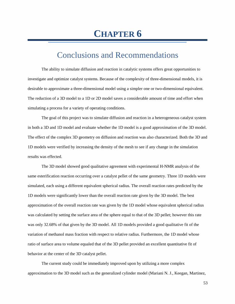
53
CHAPTER 6
Conclusions and Recommendations The ability to simulate diffusion and reaction in catalytic systems offers great opportunities to
investigate and optimize catalyst systems. Because of the complexity of three-dimensional models, it is
desirable to approximate a three-dimensional model using a simpler one or two-dimensional equivalent.
The reduction of a 3D model to a 1D or 2D model saves a considerable amount of time and effort when
simulating a process for a variety of operating conditions.
The goal of this project was to simulate diffusion and reaction in a heterogeneous catalyst system
in both a 3D and 1D model and evaluate whether the 1D model is a good approximation of the 3D model.
The effect of the complex 3D geometry on diffusion and reaction was also characterized. Both the 3D and
1D models were verified by increasing the density of the mesh to see if any change in the simulation
results was effected.
The 3D model showed good qualitative agreement with experimental H-NMR analysis of the
same esterification reaction occurring over a catalyst pellet of the same geometry. Three 1D models were
simulated, each using a different equivalent spherical radius. The overall reaction rates predicted by the
1D models were significantly lower than the overall reaction rate given by the 3D model. The best
approximation of the overall reaction rate was given by the 1D model whose equivalent spherical radius
was calculated by setting the surface area of the sphere equal to that of the 3D pellet; however this rate
was only 32.68% of that given by the 3D model. All 1D models provided a good qualitative fit of the
variation of methanol mass fraction with respect to relative radius. Furthermore, the 1D model whose
ratio of surface area to volume equaled that of the 3D pellet provided an excellent quantitative fit of
behavior at the center of the 3D catalyst pellet.
The current study could be immediately improved upon by utilizing a more complex
approximation to the 3D model such as the generalized cylinder model (Mariani N. J., Keegan, Martinez,

54
& Barreto, 2003). Furthermore, the kinetic model employed in the simulation could be immediately
improved upon by incorporating the mechanisms of adsorption into the rate law expression. Because the
kinetic parameters presented in Chapter 3 do not account for these mechanisms values from literature for
adsorption parameters would have to be used unless new kinetic experiments were devised.

55
NOMENCLATURE
av = catalyst surface area per reactor volume �1m�
A = pre-exponential factor Varies
kC = mass transfer coefficient �ms �
Ci = concentration of species i �kmolm3 �
Cis = concentration of species i on solid surface �kmolm3 �
cP = heat capacity �J
kg K�
De = effective diffusivity �m2
s�
Dfluid = fluid diffusivity �m2
s�
dp = characteristic pellet diameter [m]
d = diameter [m]
Ea = activation energy �kJ
mol�
H = enthalpy [J]
hf = heat transfer coefficient �W
m2K�
k = reaction rate constant Varies
K = reaction equilibrium constant [−]
ker = effective thermal conductivity �W
m K�
N = number of moles [moles]
p = static pressure [Pa]
r = radial coordinate [m]
T = temperature [K]
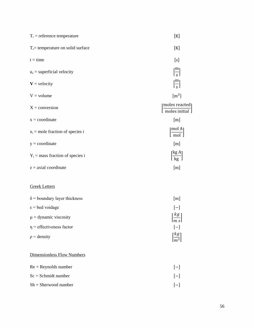
56
Tr = reference temperature [K]
Ts= temperature on solid surface [K]
t = time [s]
us = superficial velocity �ms �
V = velocity �ms �
V = volume [m3]
X = conversion �moles reactedmoles initial �
x = coordinate [m]
xi = mole fraction of species i �mol Amol �
y = coordinate [m]
Yi = mass fraction of species i �kg Akg �
z = axial coordinate [m]
Greek Letters
δ = boundary layer thickness [𝑚]
ε = bed voidage [−]
µ = dynamic viscosity �𝑘𝑔𝑚 𝑠�
η = effectiveness factor [−]
ρ = density �𝑘𝑔𝑚3�
Dimensionless Flow Numbers
Re = Reynolds number [−]
Sc = Schmidt number [−]
Sh = Sherwood number [−]

57
REFERENCES
Anderson, J. D. (1995). Computational Fluid Dynamics: The Basics with Applications. New York: McGraw-Hill, Inc.
Avci, A. K., Trimm, D. L., & Onsan, Z. I. (2001). Heterogeneous reactor modeling for simulation of catalytic oxidation and steam reforming of methane. Chemical Engineering Science , 641-649.
Dalman, M. T., Merkin, J. H., & McGreavy, C. (1986). Fluid flow and heat transfer past two spheres in a cylindrical tube. Computers and Fluids , 267-281.
Dixon, A. G., & Cresswell, D. L. (1987). Model Reduction for Two-Dimensional Catalyst Pellets with Complex Kinetics. Industrial and Engineering Chemistry Research , 2306-2312.
Dixon, A. G., Taskin, M. E., Nijemeisland, M., & Stitt, E. H. (2010). CFD Method to Couple Three-Dimensional Transport and Reaction inside Catalyst Particles to the Fixed Bed Flow Field. Industrial and Engineering Chemistry Research , 9012-9025.
DOW Ion Exchange Resins - Color Release. (2010, February 10). Retrieved 03 25, 2011, from DOW Answer Center: http://dow-answer.custhelp.com/app/answers/detail/a_id/4928/~/dow-ion-exchange-resins---color-release
du Toit, E., & Nicol, W. (2004). The rate inhibitine effect of water as a product on reactions catalysed by cation exchange resins: formation of mesityl oxide from aceton as case study. Applied Catalysis , 219-225.
Dyer, A. (2007). The Zeolite Scene - An Overview. In J. Cejka, H. van Bekkum, A. Corma, & F. Schuth, Introduction to Zeolite Science and Practice (pp. 525-554). Boston: Elsevier.
Fogler, H. S. (2006). Elements of Chemical Reaction Engineering. Boston: Prentice Hall.
Froment, G. F., & Bischoff, K. B. (1979). Chemical Reactor Analysis and Design. New York: John Wiley & Sons.
Harmer, M. A., & Sun, Q. (2001). Solid acid catalysts using ion-exchange resins. Applied Catalysis , 45-62.
Huang, J., Yijiao, J., Reddy Marthala, V. R., Wang, W., Sulikowski, B., & Hunger, M. (2007). In situ H MAS NMR investigations of the H/D exchange of alkylaromatic hydrocarbons on zeolites H-Y, La, Na-Y, and H-ZSM-5. Microporous and Mesoporous Materials , 86-90.

58
Industrial Catalysis. (n.d.). Retrieved March 20, 2011, from Johnson Matthey Catalysts: http://resources.schoolscience.co.uk/JohnsonMatthey/page14.htm
Maesen, T. (2007). The Zeolite Scene - An Overview. In J. Cejka, H. van Bekkum, A. Corma, & F. Schuth, Introduction to Zeolite Science and Practice (pp. 1-12). Boston: Elsevier.
Mariani, N. J., Keegan, S. D., Martinez, O. M., & Barreto, G. F. (2003). A One-Dimensional Equivalent Model to Evaluate Overall Reaction Rates in Catalytic Pellets. Institution of Chemical Engineers , 1033-1042.
Mariani, N. J., Keegan, S. D., Martinez, O. M., & Guillermo, F. B. (2008). On the evaluation of effective reaction rates on commercial catalyst by means of a one-dimensional modal. Catalysis Today , 770-774.
Nagaraj, A., & Mills, P. L. (2008). Analysis of Heat, Mass Transport, and Momentum Transport Effects in Complex Catalyst Shapes for Gas-Phase Heterogeneous Reactions Using Comsol Multiphysics. COMSOL Conference 2008 Proceedings. Boston.
Nijemeisland, M., & Dixon, A. G. (2001). Comparison of CFD simulations to experiment for convective heat transfer in a gas-solid fixed bed. Chemical Engineering Journal , 231-246.
Pedernera, M. N., Pina, J., Borio, D. O., & Bucala, V. (2003). Use of a heterogeneous two-dimensional model to improve the primary steam reformer performance. Chemical Engineering Journal , 29-40.
Popken, T., Gotze, L., & Gmehling, J. (2000). Reaction Kinetics and Chemical Equilibrium of Homogeneously and Heterogeneously Catalyzed Acetic Acid Esterification with Methanol and Methyl Acetate Hydrolysis. Industrial and Engineering Chemistry Research , 2601-2611.
Sie, S. T., & Kirshna, R. (1998). Process Development and Scale Up: II. Catalyst Design Strategy. Reviews in Chemical Engineering , 159-202.
Smith, J. M., Van Ness, H. C., & Abbott, M. M. (2005). Introduction to Chemical Engineering Thermodynamics. Boston: McGraw Hill.
Su, B.-L., & Norberg, V. (1997). Characterization of the Bronsted acid properties of H(Na)-Beta zeolite by infared spectroscopy and thermal analysis. Zeolites , 65-74.
Tannehill, J. C., Anderson, D. A., & Pletcher, R. H. (1997). Computational Fluid Mechanics and Heat Transfer. Washington, DC: Taylor & Francis.
Teo, H., & Saha, B. (2004). Heterogeneous catalysed esterification of acetic acid with isoamyl alcohol: kinetic studies. Journal of Catalysis , 174-182.
Zeiser, T., Lammers, P., Klemm, E., Li, Y. W., Bernsdorf, J., & Brenner, G. (2001). CFD-calculation of flow, dispersion, and reaction in a catalyst filled tube by the lattice Boltzmann method. Chemical Engineering Science , 1697-1704.

59
APPENDIX A
Gas-Liquid Chromatography Data Conversion Tables A1 through A4 present each calculation in determining the pseudo-first order rate constant for each of the four experimental conditions
described in Chapter 3. Table A5 presents each quantity used in determining the pseudo-homogeneous rate constant, activation energy, and pre-
exponential factor. The variable xi presents mole fraction data, the subscripts “AA” and “MA” refer to acetic acid and methyl acetate, respectively.
The superscripts “exp.”, “theory”, and “crctd.” refer to experimental, theoretical values, and corrected values, respectively.
Time (𝐬) 𝐱𝐀𝐀 𝐱𝐌𝐀 𝐱𝐀𝐀+𝐌𝐀
𝐞𝐱𝐩. 𝐱𝐀𝐀+𝐌𝐀𝐭𝐡𝐞𝐨𝐫𝐲 𝐱𝐀𝐀𝐜𝐫𝐜𝐭𝐝. 𝐱𝐌𝐀𝐜𝐫𝐜𝐭𝐝. Conversion
(%)
Nreacted (moles)
∂V (𝐦𝟑)
V (𝐦𝟑)
CAA
(𝐤𝐦𝐨𝐥𝐦𝟑 )
CMA
(𝐤𝐦𝐨𝐥𝐦𝟑 )
ln(CAA) (𝐤𝐦𝐨𝐥𝐦𝟑 )
ln(CMA) (𝐤𝐦𝐨𝐥𝐦𝟑 )
0 0.0000 0.0909 0.0909 0.07169 0.0000 0.1153 0.0000 0.0000 0.000E+00 2.100E-04 0.0000 2.6748 --- 0.9839
1800 0.0081 0.0888 0.0969 0.07169 0.01027 0.1126 0.02310 0.1126 -3.058E-08 2.100E-04 0.2384 2.6134 -1.4339 0.9606
3600 0.0036 0.0876 0.0912 0.07169 0.00456 0.1111 0.03630 0.1769 -4.806E-08 2.100E-04 0.1060 2.5783 -2.2447 0.9471
5400 0.0135 0.0852 0.0987 0.07169 0.01712 0.1080 0.06271 0.3056 -8.301E-08 2.099E-04 0.3974 2.5081 -0.9228 0.9195
7200 0.0119 0.083 0.0949 0.07169 0.01509 0.1052 0.08691 0.4235 -1.150E-07 2.099E-04 0.3504 2.4437 -1.0488 0.8935
9000 0.015 0.0802 0.0952 0.07169 0.01902 0.1017 0.1177 0.5737 -1.558E-07 2.098E-04 0.4417 2.3617 -0.8171 0.8594
10800 0.0186 0.0788 0.0974 0.07169 0.02358 0.09992 0.1331 0.6487 -1.762E-07 2.098E-04 0.5478 2.3207 -0.6019 0.8419
12600 0.0209 0.0764 0.0973 0.07169 0.02650 0.09687 0.1595 0.7774 -2.112E-07 2.098E-04 0.6156 2.2504 -0.4851 0.8111
14400 0.0192 0.0756 0.0948 0.07169 0.02435 0.09586 0.1683 0.8203 -2.228E-07 2.098E-04 0.5656 2.2270 -0.5699 0.8006
Table A1: 40°C, 4 g Catalyst GLC Data Conversion

60
Time (𝐬) 𝐱𝐀𝐀 𝐱𝐌𝐀 𝐱𝐀𝐀+𝐌𝐀
𝐞𝐱𝐩. 𝐱𝐀𝐀+𝐌𝐀𝐭𝐡𝐞𝐨𝐫𝐲 𝐱𝐀𝐀𝐜𝐫𝐜𝐭𝐝. 𝐱𝐌𝐀𝐜𝐫𝐜𝐭𝐝. Conversion
(%)
Nreacted (moles)
∂V (𝐦𝟑)
V (𝐦𝟑)
CAA
(𝐤𝐦𝐨𝐥𝐦𝟑 )
CMA
(𝐤𝐦𝐨𝐥𝐦𝟑 )
ln(CAA) (𝐤𝐦𝐨𝐥𝐦𝟑 )
ln(CMA) (𝐤𝐦𝐨𝐥𝐦𝟑 )
0 0 0.095 0.095 0.07169 0.00000 0.1259 0.0000 0.0000 0.0000 2.100E-04 0.0000 2.922 1.072
1800 0.0087 0.1055 0.1142 0.07169 0.01153 0.1398 0.1105 0.5386 -1.463E-07 2.099E-04 0.2677 3.247 -1.318 1.178
3600 0.018 0.0981 0.1161 0.07169 0.02385 0.1300 0.03263 0.1590 -4.320E-08 2.100E-04 0.5537 3.017 -0.5912 1.104
5400 0.0227 0.0918 0.1145 0.07169 0.03008 0.1217 0.03368 0.1642 -4.459E-08 2.100E-04 0.6982 2.824 -0.3592 1.038
7200 0.0257 0.0885 0.1142 0.07169 0.03406 0.1173 0.06842 0.3334 -9.057E-08 2.099E-04 0.7907 2.723 -0.2348 1.002
9000 0.0337 0.0854 0.1191 0.07169 0.04466 0.1132 0.1011 0.4925 -1.338E-07 2.099E-04 1.037 2.628 0.03637 0.9662
10800 0.0272 0.0871 0.1143 0.07169 0.03605 0.1154 0.08316 0.4053 -1.101E-07 2.099E-04 0.8369 2.680 -0.1780 0.9858
12600 0.0415 0.0774 0.1189 0.07169 0.05500 0.1026 0.1853 0.9029 -2.452E-07 2.098E-04 1.278 2.383 0.2451 0.8684
14400 0.0469 0.074 0.1209 0.07169 0.06215 0.09806 0.2211 1.077 -2.926E-07 2.097E-04 1.444 2.279 0.3676 0.8237
Table A2: 50°C, 4 g Catalyst GLC Data Conversion

61
Time (𝐬) 𝐱𝐀𝐀 𝐱𝐌𝐀 𝐱𝐀𝐀+𝐌𝐀
𝐞𝐱𝐩. 𝐱𝐀𝐀+𝐌𝐀𝐭𝐡𝐞𝐨𝐫𝐲 𝐱𝐀𝐀𝐜𝐫𝐜𝐭𝐝. 𝐱𝐌𝐀𝐜𝐫𝐜𝐭𝐝. Conversion
(%)
Nreacted (moles)
∂V (𝐦𝟑)
V (𝐦𝟑)
CAA
(𝐤𝐦𝐨𝐥𝐦𝟑 )
CMA
(𝐤𝐦𝐨𝐥𝐦𝟑 )
ln(CAA) (𝐤𝐦𝐨𝐥𝐦𝟑 )
ln(CMA) (𝐤𝐦𝐨𝐥𝐦𝟑 )
0 0.0000 0.095 0.095 0.07169 0.00000 0.1259 0.0000 0.0000 0.0000 2.100E-04 0.0000 2.922 ---- 1.072
1800 0.025 0.0788 0.1038 0.07169 0.03313 0.1044 0.1705 0.8310 -2.257E-07 2.098E-04 0.7697 2.426 -0.2618 0.8862
3600 0.0124 0.081 0.0934 0.07169 0.01643 0.1073 0.1474 0.7182 -1.951E-07 2.098E-04 0.3817 2.493 -0.9631 0.9136
5400 0.0387 0.0719 0.1106 0.07169 0.05128 0.09528 0.2432 1.185 -3.219E-07 2.097E-04 1.192 2.215 0.1756 0.7950
7200 0.0499 0.067 0.1169 0.07169 0.06613 0.08879 0.2947 1.436 -3.902E-07 2.096E-04 1.537 2.064 0.4301 0.7248
9000 0.0561 0.0605 0.1166 0.07169 0.07434 0.08017 0.3632 1.770 -4.807E-07 2.095E-04 1.729 1.865 0.5477 0.6232
10800 0.0684 0.0549 0.1233 0.07169 0.09064 0.07275 0.4221 2.057 -5.588E-07 2.094E-04 2.109 1.693 0.7463 0.5264
12600 0.0635 0.0515 0.115 0.07169 0.08415 0.06825 0.4579 2.231 -6.061E-07 2.094E-04 1.958 1.588 0.6722 0.4627
Table A3: 60°C, 4 g Catalyst GLC Data Conversion

62
Time (𝐬) 𝐱𝐀𝐀 𝐱𝐌𝐀 𝐱𝐀𝐀+𝐌𝐀
𝐞𝐱𝐩. 𝐱𝐀𝐀+𝐌𝐀𝐭𝐡𝐞𝐨𝐫𝐲 𝐱𝐀𝐀𝐜𝐫𝐜𝐭𝐝. 𝐱𝐌𝐀𝐜𝐫𝐜𝐭𝐝. Conversion
(%)
Nreacted (moles)
∂V (𝐦𝟑)
V (𝐦𝟑)
CAA
(𝐤𝐦𝐨𝐥𝐦𝟑 )
CMA
(𝐤𝐦𝐨𝐥𝐦𝟑 )
ln(CAA) (𝐤𝐦𝐨𝐥𝐦𝟑 )
ln(CMA) (𝐤𝐦𝐨𝐥𝐦𝟑 )
0 0.0000 0.095 0.095 0.07169 0.0000 0.1259 0.0000 0.0000 0.0000 2.100E-04 0.00000 2.922 --- 1.072
1800 0.0458 0.079 0.1248 0.07169 0.06069 0.1047 0.1684 0.8208 -2.229E-07 2.098E-04 1.410 2.432 0.3436 0.8887
3600 0.0691 0.0652 0.1343 0.07169 0.09157 0.08640 0.3137 1.529 -4.152E-07 2.096E-04 2.129 2.009 0.7558 0.6977
5400 0.0901 0.0524 0.1425 0.07169 0.1194 0.06944 0.4484 2.185 -5.936E-07 2.094E-04 2.779 1.616 1.022 0.4800
7200 0.0995 0.0421 0.1416 0.07169 0.1319 0.05579 0.5568 2.714 -7.371E-07 2.093E-04 3.071 1.299 1.122 0.2618
9000 0.1057 0.0341 0.1398 0.07169 0.1401 0.04519 0.6411 3.124 -8.486E-07 2.092E-04 3.264 1.053 1.183 0.05158
10800 0.124 0.0292 0.1532 0.07169 0.1643 0.03870 0.6926 3.375 -9.169E-07 2.091E-04 3.830 0.9019 1.343 -0.1032
Table A4: 60°C, 8 g Catalyst GLC Data Conversion

63
TABLE A5: QUANTITIES USED TO CALCULATE KINETIC PARAMETERS
T (s)
mcatalyst (g)
k' (𝐬−𝟏)
k' ( 𝐦𝟑
𝐬 𝐤𝐠𝐜𝐚𝐭𝐚𝐥𝐲𝐬𝐭)
k ( 𝐦𝟔
𝐬 𝐤𝐦𝐨𝐥𝐤𝐠𝐜𝐚𝐭𝐚𝐥𝐲𝐬𝐭)
A ( 𝐦𝟔
𝐬 𝐤𝐦𝐨𝐥𝐤𝐠𝐜𝐚𝐭𝐚𝐥𝐲𝐬𝐭)
313.15 4 1.345*10-5 7.060*10-7 3.335*10-8 -17.22
323.15 4 2.065*10-5 1.084*10-6 5.121*10-8 -16.79
333.15 4 4.634*10-5 2.433*10-6 1.148*10-7 -15.98
333.15 8 1.118*10-4 2.935*10-6 2.494*10-7 -15.20

64
APPENDIX B
Sample Gambit Journal / Journal File for GAMBIT 2.4.6, Database 2.4.4, ntx86 SP2007051421
/ Identifier "default_id3100"
/ File opened for write Thu Jan 13 19:40:29 2011.
identifier name "Catalyst System" new nosaveprevious
volume create height 0.01 radius1 0.0175 radius2 0.0175 radius3 0.0175 offset \
0 0 0.005 zaxis frustum
volume create height 0.01 radius1 0.00425 radius2 0.00425 radius3 0.00425 \
offset 0 0 0.005 zaxis frustum
volume move "volume.2" offset -0.0085 0 0
volume cmove "volume.2" multiple 1 offset 0.017 0 0
volume cmove "volume.3" multiple 1 offset -0.0085 0.0085 0
volume cmove "volume.3" multiple 1 offset -0.0085 -0.0085 0
volume cmove "volume.3" multiple 1 offset -0.0085 0 0
volume cmove "volume.6" multiple 1 offset 0.012374 0.012374 0
volume cmove "volume.6" multiple 1 offset -0.012374 0.012374 0
volume cmove "volume.6" multiple 1 offset 0.012374 -0.012374 0
volume move "volume.6" offset -0.012374 -0.012374 0
volume subtract "volume.1" volumes "volume.8" "volume.4" "volume.7" \
"volume.3" "volume.9" "volume.5" "volume.2" "volume.6"

65
volume create height 0.27 radius1 0.02 radius2 0.02 radius3 0.02 offset 0 0 \
0.135 zaxis frustum
volume move "volume.1" offset 0 0 0.07
volume subtract "volume.2" volumes "volume.1" keeptool
face modify "face.7" label "PELLET HOLE (X)"
face modify "face.10" label "PELLET HOLE (Y)"
face modify "face.5" label "PELLET HOLE (-X)"
face modify "face.13" label "PELLET HOLE (-Y)"
face modify "face.29" label "PELLET FACE (-Z)"
face modify "face.34" label "PELLET FACE (Z)"
face modify "face.2" label "PELLET WALL (Y)"
face modify "face.31" label "PELLET WALL (X)"
face modify "face.30" label "PELLET WALL (-X)"
face modify "face.33" label "PELLET WALL (-Y)"
face modify "face.19" label "PELLET WALL (I)"
face modify "face.25" label "PELLET WALL (IV)"
face modify "face.16" label "PELLET WALL (III)"
face modify "face.22" label "PELLET WALL (II)"
face modify "face.45" label "REACTOR HOLE (X)"
face modify "face.47" label "REACTOR FACE (-Z)"
face modify "face.49" label "REACTOR HOLE (Y)"
face modify "face.41" label "REACTOR HOLE (-X)"
face modify "face.42" label "REACTOR HOLE (-Y)"
face modify "face.39" label "REACTOR FACE (Z)"
face modify "face.51" label "REACTOR WALL (Y)"
face modify "face.44" label "REACTOR WALL (X)"

66
face modify "face.40" label "REACTOR WALL (-Y)"
face modify "face.48" label "REACTOR WALL (-X)"
face modify "face.46" label "REACTOR WALL (I)"
face modify "face.43" label "REACTOR WALL (IV)"
face modify "face.38" label "REACTOR WALL (III)"
face modify "face.50" label "REACTOR WALL (II)"
face modify "face.35" label "VELOCITY INLET"
face modify "face.36" label "TUBE WALL"
face modify "face.37" label "PRESSURE OUTLET"
face connect "PELLET HOLE (-X)" "REACTOR HOLE (-X)" real
face connect "PELLET WALL (Y)" "REACTOR WALL (Y)" real
face connect "PELLET HOLE (X)" "REACTOR HOLE (X)" real
face connect "PELLET HOLE (Y)" "REACTOR HOLE (Y)" real
face connect "PELLET HOLE (-Y)" "REACTOR HOLE (-Y)" real
face connect "PELLET WALL (I)" "REACTOR WALL (I)" real
face connect "PELLET WALL (II)" "REACTOR WALL (II)" real
face connect "PELLET WALL (III)" "REACTOR WALL (III)" real
face connect "PELLET WALL (IV)" "REACTOR WALL (IV)" real
face connect "PELLET WALL (-X)" "REACTOR WALL (-X)" real
face connect "PELLET WALL (X)" "REACTOR WALL (X)" real
face connect "PELLET FACE (-Z)" "REACTOR FACE (-Z)" real
face connect "PELLET FACE (Z)" "REACTOR FACE (Z)" real
face connect "PELLET WALL (-Y)" "REACTOR WALL (-Y)" real
physics create "WALL" btype "WALL" face "TUBE WALL"
physics create "PELLET" btype "WALL" face "TUBE WALL" "PELLET WALL (Y)" \
"PELLET HOLE (-X)" "PELLET HOLE (X)" "PELLET HOLE (Y)" "PELLET HOLE (-Y)" \

67
"PELLET WALL (III)" "PELLET WALL (I)" "PELLET WALL (II)" "PELLET WALL (IV)" \
"PELLET FACE (-Z)" "PELLET WALL (-X)" "PELLET WALL (X)" "PELLET WALL (-Y)" \
"PELLET FACE (Z)"
physics create btype "VELOCITY_INLET" face "VELOCITY INLET"
physics create "PRESSURE O+UTLET" btype "PRESSURE_OUTLET" face \
"PRESSURE OUTLET"
physics modify "velocity_inlet.2" btype label "VELOCITY INLET" face \
"VELOCITY INLET"
face mesh "PELLET WALL (Y)" "PELLET HOLE (-X)" "PELLET HOLE (X)" \
"PELLET HOLE (Y)" "PELLET HOLE (-Y)" "PELLET WALL (III)" "PELLET WALL (I)" \
"PELLET WALL (II)" "PELLET WALL (IV)" "PELLET FACE (-Z)" "PELLET WALL (-X)" \
"PELLET WALL (X)" "PELLET WALL (-Y)" "PELLET FACE (Z)" triangle size \
0.0005
volume mesh "volume.2" tetrahedral size 0.01
volume mesh "volume.1" tetrahedral size 0.001
physics create "FLUID" ctype "FLUID" volume "volume.2"
physics create "SOLID" ctype "SOLID" volume "volume.1"
save
export fluent5 "Catalyst System.msh"

68
APPENDIX C
3D Simulation Convergence Plots
FIGURE 1911: UNREFINED MESH CONVERGENCE PLOT

69
FIGURE 120: REFINED MESH CONVERGENCE PLOT