NASA TECHNICAL NOTE NASA TN D-3645 --- (5, m

w- = a *o - 0

==E T n

z LOAN COPY: RETURN g c AFWL (v1'LlL-2) p G $ e

-_ar uh - 2

4 - E z

- 0 - 6

KIRTLAND A.FB, I\! M "'m n -

COMPARISON OF ONE- AND TWO-DIMENSIONAL HEAT-TRANSFER CALCULATIONS I N CENTRAL FIN-TUBE RADIATORS

by Norbert 0. Stockmun, Edwurd C. Bittner, und Earl L. Spragne

Lewis Research Center CZeveZund, Ohio

N A T I O N A L A E R O N A U T I C S A N D SPACE A D M I N I S T R A T I O N W A S H I N G T O N , D. C. S E P T E M B E R 1966 x i

https://ntrs.nasa.gov/search.jsp?R=19660028012 2018-08-12T23:11:59+00:00Z

TECH LIBRARY KAFB, NM

NASA TN D-3645

COMPARISON OF ONE- AND TWO-DIMENSIONAL HEAT-TRANSFER

CALCULATIONS IN CENTRAL FIN-TUBE RADIATORS

By Norber t 0. Stockman, Edward C. Bi t tner , and E a r l L. Sprague

Lewis R e s e a r c h Center Cleveland, Ohio

NATIONAL AERONAUTICS AND SPACE ADMINISTRATION

For sale by the Clearinghouse for Federal Scientific and Technical Information Springfield, Virginia 22151 - Price $2.00

COMPARISON OF ONE- AND TWO-DIMENSIONAL HEAT-TRANSFER

CALCULATIONS IN CENTRAL FIN-TUBE RADIATORS

by Norbert 0. Stockman, Edward C. Bittner, and Earl L. Sprague

Lewis Research Center

SUMMARY

An analysis is given of the two-dimensional heat transfer, including gray body radiant interchange, in the cross section of a central fin-tube radiator panel. analysis are used to evaluate several one-dimensional methods of varying complexity for calculating the heat rejection rate of a central fin-tube radiator panel. Most methods gave good agreement with the two-dimensional results. In view of the excellent agree- ment of one of the simpler methods which neglects tube wall temperature drop and ac- counts for radiant interchange between fin and tube simply by using the projected area of the tube, it seems unwarranted to use the more complex methods which gave no better agreement. Details of the numerical method of solution of the two-dimensional equations are given in an appendix.

Results of this

INTRODUCTION

Electric power generation systems for space applications must reject large amounts of waste heat. At the present state of the art, the most likely method of rejecting this heat is by means of a radiator that utilizes some sort of fin and tube configuration. Var- ious fin and tube combinations have been proposed, but only the central fin-tube geometry (fig. 1) will be considered in this report. Since the radiator represents a large portion of the powerplant weight, it must be accurately designed. Radiator design calculations are usually based on the assumption of one-dimensional heat transfer in the cross section of the fin and tube panel. Several different methods have been used to compute the heat rejection from central fin-tube panels (e. g., refs. 1 to 8). These methods contain vary- ing degrees of complexity, and it is not obvious which methods are more accurate.

fin-tube heat transfer were carried out at NASA Lewis Research Center.. These calcula- In order to evaluate the one-dimensional methods, two-dimensional calculations of

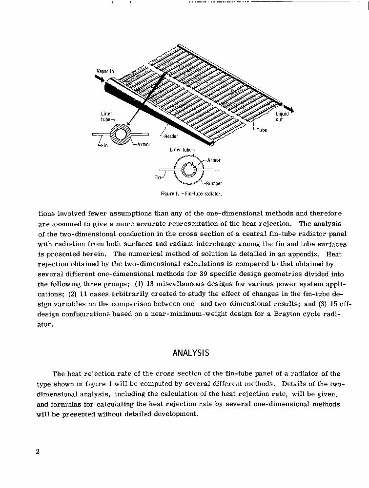
. ... Liner tube,

Fi

Figure 1. - Fin-tube radiator.

tions involved fewer assumptions than any of the one-dimensional methods and therefore are assumed to give a more accurate representation of the heat rejection. The analysis of the two-dimensional conduction in the cross section of a central fin-tube radiator panel with radiation from both surfaces and radiant interchange among the fin and tube surfaces is presented herein. The numerical method of solution is detailed in an appendix. Heat rejection obtained by the two-dimensional calculations is compared to that obtained by several different one-dimensional methods for 39 specific design geometries divided into the following three groups: (1) 13 miscellaneous designs for various power system appli- cations; (2) 11 cases arbitrarily created to study the effect of changes in the fin-tube de- sign variables on the comparison between one- and two-dimensional results; and (3) 15 off- design configurations based on a near-minimum-weight design for a Brayton cycle radi- ator.

ANALYSIS

The heat rejection rate of the cross section of the fin-tube panel of a radiator of the type shown in figure 1 will be computed by several different methods. Details of the two- dimensional analysis, including the calculation of the heat rejection rate, will be given, and formulas for calculating the heat rejection rate by several one-dimensional methods will be presented without detailed development.

2

Assumptions

All the methods (one- and two-dimensional) are based on steady-state heat conduction in the cross section of the fin and tube, radiation from both fin and tube surfaces, and the following specific assumptions (other more restrictive assumptions are required for cal- culating heat rejection rate by the various one-dimensional methods, and these will be given later with the formulas for heat rejection rate for each method):

tubes. (1) The radiator is infinitely long and made up of an infinite number of identical finned

(2) The inside tube wall is isothermal both longitudinally and circumferentially. (3) The tubes and fins are made of the same material, and the material properties

are assumed invariant with temperature. (4) If there is a liner (as in fig. l), it is of the same material as the tube and is in

perfect thermal contact with the tube. (5) Incident radiation from external sources such as Sun and planets and adjacent ve-

hicle components is accounted for by a completely encompassing surface of constant tem- perature called the equivalent sink temperature Ts (ref. 9). This temperature is as- sumed to be the same on both sides of the radiator.

perature. (6) Radiating surfaces are gray at a prescribed value of emittance invariant with tem-

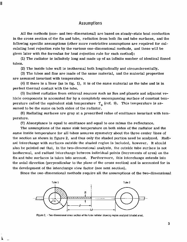
(7) Absorptance is equal to emittance and equal to one minus the reflectance. The assumptions of the same sink temperature on both sides of the radiator and the

same inside temperature for all tubes assures symmetry about the three center lines of the section as shown in figure 2, and thus only the shaded portion need be analyzed. Radi- ant interchange with surfaces outside the shaded region is included, however. It should also be pointed out that, in the two-dimensional analysis, the outside tube surface is not isothermal, and radiant interchange between individual points (increments of area) on the fin and tube surfaces is taken into account. Furthermore, this interchange extends into the axial direction (perpendicular to the plane of the cross section) and is accounted for in the development of the interchange view factor (see next section).

Since the one-dimensional methods require all the assumptions of the two-dimensional

Tube 1 Tube 2

I 2 t I fs L

Figure 2. -Two-dimensional cross section of fin-tube radiator showing region analyzed (shaded area).

3

plus additional ones, the two-dimensional results are the limit to which the one- dimensional results tend with increasing refinement. Thus the two-dimensional heat re- jection is used as the standard to evaluate the relative merits of the one-dimensional methods. In the next section, the differential equation and boundary conditions governing the two-dimensional heat transfer in the fin cross section under the assumptions listed previously will be presented.

Equation's and Boundary Conditions

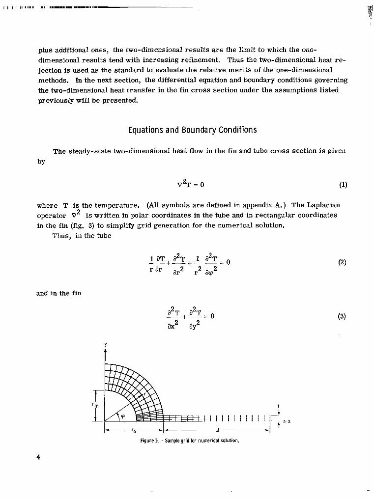
The steady-state two-dimensional heat flow in the fin and tube cross section is given

(1) 2 V T = O

where T is the temperature. (All symbols are defined in appendix A,) The Laplacian operator V2 is written in polar coordinates in the tube and in rectangular coordinates in the fin (fig. 3) to simplify grid generation for the numerical solution.

Thus, in the tube

and in the fin

2 2 a T + a T = 0 ;hr2 ay2

Y

t

Figure 3. - Sample grid for numerical solution.

4

These are the two partial differential equations which must be solved. The solutions must also satisfy the following boundary conditions. Along the inside tube wall at r = rin, the temperature is prescribed:

There is no heat flow across the lines cp = 0 and cp = (n/2) in the tube because of sym- metry, so

Also, because of symmetry, there is no heat flow across the lines y = 0 and x = Q + ro in the fin, so that

= o x=Q +r 0

On the surface of the tube at r = ro there is radiation to space where the sink tem- perature is Ts and interchange with surfaces of the fin and the adjacent tube. The boundary condition for net heat rejection from the tube surface can be written as

4 = e a T 4 - ( Y H = E ( O T - H)

0 r =r

where E is the emittance, (Y is the absorptance of the surface, and H is the incident radiation including that from the sink and from other parts of the raditor surface. Simi- larly on the surface of the fin at y = t, the net heat rejection is

aT 4

aY -k-=E(OT - H)

Since that part of the incident radiation H contributed by the radiator surface is unknown and must be determined as part of the solution of the problem, H must be written in a form in which the radiator surface radiation appears explicitly. The equation for H, derived in appendix B, is

5

where BdA is the radiosity (the total energy per unit time and unit area) leaving an ele- ment dA on the fin-tube surface and for a particular element dA* is given by

Substituting equation (8) into equation (9) and replacing p by 1 - E yield

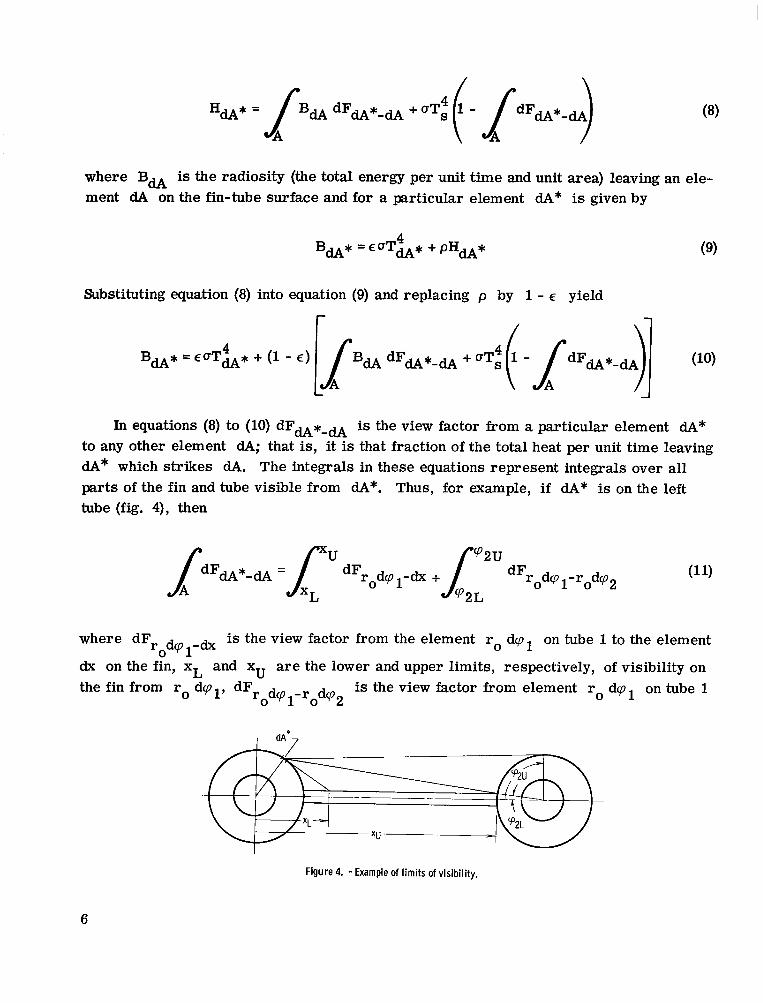
In equations (8) to (10) dFdA*-dA is the view factor from a particular element dA* to any other element dA; that is, it is that fraction of the total heat per unit time leaving dA* which strikes dA. The integrals in these equations represent integrals over all parts of the fin and tube visible from dA*. Thus, for example, i f dA* is on the left tube (fig. 4), then

is the view factor from the element ro dql on tube 1 to the element where dF

dx on the fin, xL and xu are the lower and upper limits, respectively, of visibility on the fin from ro dP1, dFrodql-rodq, is the view factor from element ro dql on tube 1

row 1-dx

Figure 4. -Example of limits of visibility.

6

to element ro dq2 on tube 2, and q2L and qZu are the lower and upper limits, re- spectively, of visibility on tube 2 from ro dql. several fin-tube radiator configurations are given in ref. 10.)

(View factors and limits of visibility for

It should be noted that the areas here (and heat rejection rates later) are per unit ' axial length. This is to avoid infinite quantities since the axial length is assumed infinite.

The view factors, however, are actually between elements of area of infinite length. (This presents no problem since view factors are fractional quantities and may be defined for

is that portion of the radiation infinite areas.) For example, the view factor dF

leaving the area ro dql by infinite length on tube 1 and striking the area dx by infinite length on the fin. It can be seen that the radiation leaving the surface at a certain axial location on the tube but striking a different axial location on the fin is accounted for in the view factor.

a , and t and the temperatures Tin and Ts determine the temperature distribution throughout the fin and tube. Equations (2) and (3) are differential equations in T; equa- tion (10) is an integral equation in B; and T and B a re related through equations (7) and (8). The equations were solved numerically on an IBM 7094 using a finite difference block overrelaxation method. Details of the numerical method of solution a re given in appendix C.

r,dq 1-dx

Equations (2) to (8) and equation (10) in addition to the prescribed geometry rin, ro,

Heat Rejection

The temperature distribution resulting from the solution of the equations of the pre- ceding section is used to obtain a net heat rejection rate. The net heat rejection rate is also calculated by several one-dimensional methods for comparison with the two- dimensional results.

tained, the net heat rejected Q2D by the radiator per unit axial length for one quadrant can be obtained by integrating the left-hand side of equation (7a) over the tube outer sur- face and the left-hand side of equation (7b) over the fin outer surface; that is,

Two-dimensional. - Once the two-dimensional temperature distribution has been ob-

One-dimensional. - Several one-dimensional methods of calculating the net heat re- jection rate will be considered. The formula and a brief description of each method,

7

which will hereinafter be referred to by i ts number, follows. All methods are based on the assumptions of constant tube outer surface temperature and of one-dimensional heat conduction in a radiating fin. The conduction in the fin is accounted for by a fin efficiency or an overall efficiency. The fin efficiency depends, in general, on two dimensionless parameters: the conductance parameter h = caTbl /kt, and the sink temperature ratio Ts/Tb. The temperature Tb is the fin base temperature and is equal to To or T. in depending on.whether or not the tube wall temperature drop is taken into account. When radiant interchange with the tube is taken into account, an overall efficiency is used that depends on h and Ts/Tb and also on a third parameter, the fin-tube profile ratio Q/ro.

The items that differ from method to method are whether or not a radial one- dimensional temperature drop across the tube is considered (i. e. , whether Tb equals T or Tin); how radiant interchange between the radiator surfaces is accounted for, i f at all; what area is used for the tube radiating surface; and how nonblackbody effects ( E )

are handled. In all methods except (6), the nonblackbody effect is handled simply by in- troducing E into the formula for &. The methods, which follow, are summarized in table I.

3 2

0

Method 1:

Q~ = €0 (T!~ - T:) (llinl + - ro 2 " )

where qin is the fin efficiency based on a fin base temperature equal to Tin. Fin effi- ciency for this and the next three methods includes the effect of the sink temperature Ts but not the effect of interchange with the adjacent tubes.

is neglected, and the actual area of the tube is used. The fin efficiency qin is a function primarily of hin and secondarily of Ts/Tin and can be obtained from reference 9.

No temperature drop in the tube is considered (i. e. , Tb = Tin), radiant interchange

Method 2:

This is the same actual area.

as method 1 except that the tube projected area is used instead of the

8

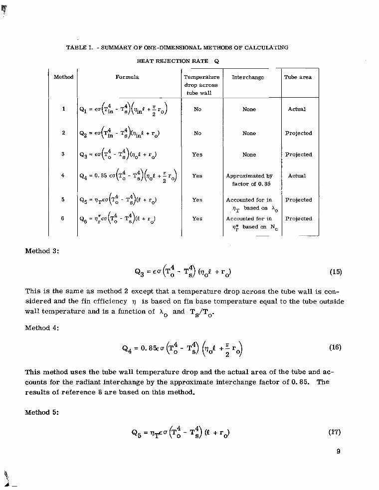
TABLE I. - SUMMARY OF ONE-DIMENSIONAL METHODS OF CALCULATING

Method

1

2

3

4

5

6

HEAT REJECTION RATE Q

Formula remperature drop across tube wall

No

No

Yes

Yes

Yes

Yes

Interchange

None

None

None

Approximated by factor of 0.85

Accounted for in qT based on Xo

q: based on Nc Accounted for in

hbe area

Actual

Projected

Projected

Actual

Projected

Projected

Method 3:

This is the same as method 2 except that a temperature drop across the tube wall is con- sidered and the fin efficiency 7 is based on fin base temperature equal to the tube outside wall temperature and is a function of Xo and Ts/To.

Method 4:

This method uses the tube wall temperature drop and the actual area of the tube and ac- counts for the radiant interchange by the approximate interchange factor of 0.85. The results of reference 8 are based on this method.

Method 5:

This method uses the temperature drop in the tube and the projected area of the tube. Both the radiant interchange and the fin temperature distribution are accounted for by an overall effectiveness vT which is a function of A,, Ts/To, and Q/ro (see, e. g., refs. 4 and 6).

Method 6 :

This method is similar to method 5 except that r]: is for a blackbody and is based on Nc instead of X where Nc = ho/c, and the nonblackbody effect is accounted for by an apar-

0' - ent emissivity E . The apparent emissivity accounts for the multiple reflections among the fin and tube surfaces by considering the fin and tubes to be an isothermal cavity of specified local surface emittance E . The apparent emissivity is a function of E (held constant in this report), Q/ro, and Ts/To, while r]: is a function of Nc, Q/ro, and Ts/To. This method is developed in reference 5.

Overall Radiator Efficiency

The heat rejection rates calculated by both the one-dimensional and two-dimensional analyses are normalized by dividing by an "ideal" heat rejection rate Qid to form a so- called radiator or heat rejection efficiency; thus,

Q r] =-

Qid (19)

rr llle advantage of comparing all the analyses on the basis of r] is that the resulting values always lie between 0 and 1 (except method 1 in one case) regardless of the size or temper- ature level of the radiator section. The normalizing factor was arbitrarily chosen as

that is, the ideal heat rejection rate is based on the inside wall temperature and the pro- jected area of the tube.

An additional advantage for the use of Qid is that the efficiency for the one- dimensional analyses can be expressed in terms of nondimensional parameters, and

10

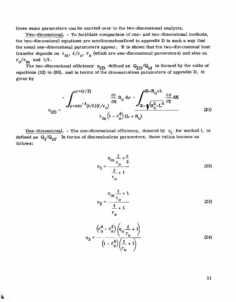
these same parameters can be carried over to the two-dimensional analysis.

the two-dimensional equations are nondimensionalized in appendix D in such a way that the usual one-dimensional parameters appear. It is shown that the two-dimensional heat transfer depends on Xin, Q/ro, O s (which are one-dimensional parameters) and also on

- Two-dimensional. -___ - To facilitate comparison of one- and two-dimensional methods,

ro/rin and t/Q.

equations (12) to (20), and in terms of the dimensionless parameters of appendix D, is given by

The two-dimensional efficiency q2D defined as Q2D/Qid is formed by the ratio of

One-dimensional. - The one-dimensional efficiency, denoted by qi for method i, is defined as Qi/Qid. In terms of dimensionless parameters, these ratios become as follows:

P a 2

+- “in - rO “1 =

Q - + 1

Q vin- + 1 rO “2 =

Q - + 1 0

r

11

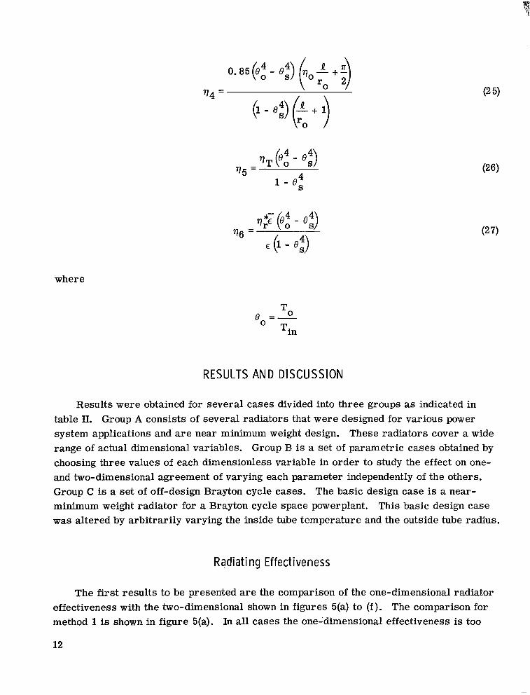
714 =

+j 2

where

RESULTS AND DlSCU SSlON

Results were obtained for several cases divided into three groups as indicated in table II. Group A consists of several radiators that were designed for various power system applications and a r e near minimum weight design. These radiators cover a wide range of actual dimensional variables. Group B is a set of parametric cases obtained by choosing three values of each dimensionless variable in order to study the effect on one- and two-dimensional agreement of varying each parameter independently of the others. Group C is a set of off-design Brayton cycle cases. The basic design case is a near- minimum weight radiator for a Brayton cycle space powerplant. This basic design case was altered by arbitrarily varying the inside tube temperature and the outside tube radius.

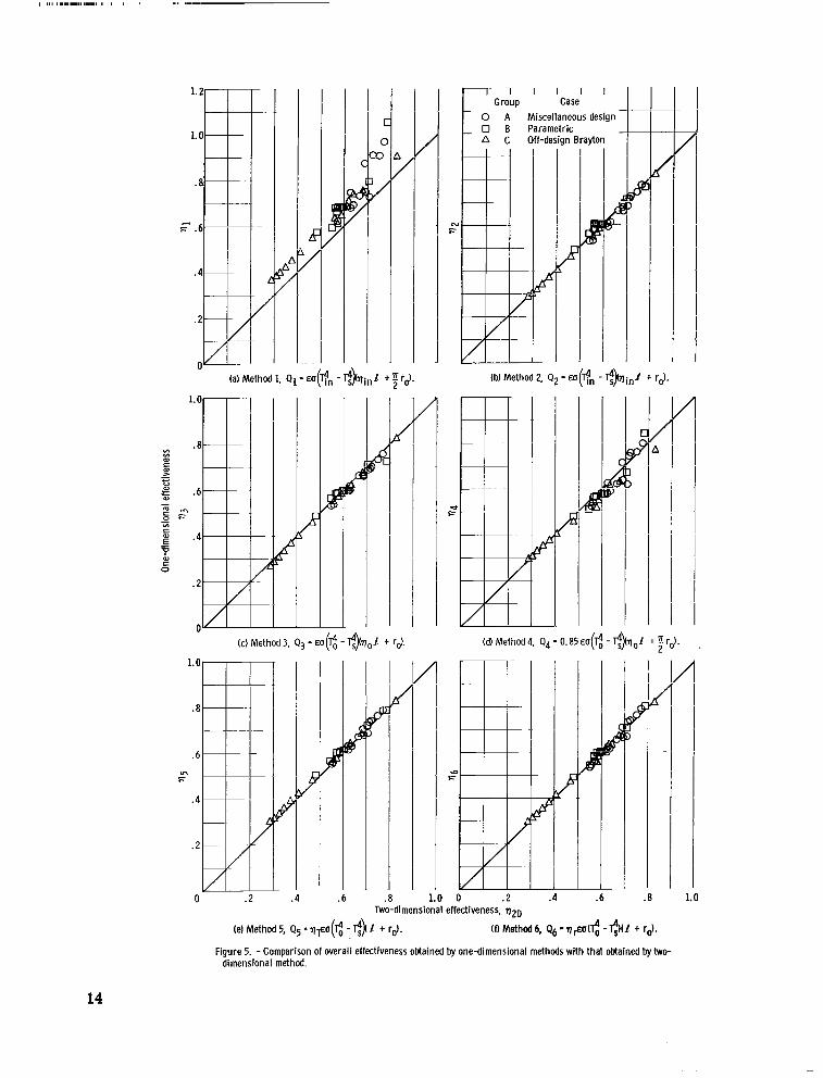
Radiating Effectiveness

The first results to be presented are the comparison of the one-dimensional radiator effectiveness with the two-dimensional shown in figures 5(a) to (f) . The comparison for method 1 is shown in figure 5(a). In all cases the one-'dimensional effectiveness is too

12

link Imper- iture ratio,

@S

El rial

Emit- tance,

E

Temper ature, inside tube wall,

Tin* aR

8.6 -4 .5 8.6 -3.4 8.6 -4 .4

11.2 -3 .5 11.1 -3.6

19.6 -3.3 2.6 -3.6

25.4 .7 26.0 . 4 26.7 . 5

9 . 8 - . 5 26.4 - . l 20.8

-4.5 -7.7 -3 .4 -7.7 -4.4 -7.8 -3.7 -5.7 -3.8 -5.7

-4.7 . 1 -3.7-12.8 -2 .2 3 .5 -3 .0 3.5 -3 .3 3.5

-.7-7.0 -3 .4 3.9

- . 9 - 2 . 5 1 .1

2.0 -3.8 1 . 3 -3 .2 2 . 3 -3.7 - . 3 -2.2 - . 4 -2.3

1 . 5 . 9 3.3 -5.6 2 .0 2 . 4 2 . 3 2 .6 2 .7 2 .8

. 6 -1.4 2 .4 2 . 7 1 . 4 1 . 5

3.5 1 . 6 2 . 0 .6 5 . 0 3.0 - . l 1 .7 3 . 2 0

2.2 - . 4 4 .5 2.6 6 . 4 4 . 5 2 . 3 . 4 3.9 1 . 8 3.5 1 .6

~

Parametric cases (B)

Off-design Brayton cases (C)

1.001 ,864 ,705

1.50 1.54

1.39 ,503 ,499 ,740 ,924

,623 ,804 ,569

1.00 ,884 ,705

1.50 1.54

1.38 ,502 .487 .719 ,894

.622 ,781 ,561

1 2 3 A l 4 % 5 A l

6 S S 7 A l

9 % 10

11 12 13

A1 A1

8 B e

Cb

Al Cb Be

1 5 . 7 1 . 8 12.7 1 . 1 19 .5 2 . 5 33.8 -2 .5 9 . 5 3.0

13.7 . 1 17.4 3.4 20.0 5 . 6 13.9 . 3 1 6 . 3 2 . 0 1 5 . 6 1 . 8

0 . 9 -2.6 . 6 - 4 . 7 .7 - . 3

-8.4 7 . 0 2.6 -7 .2

- .4 -3 .8 1 .9 -1.7 3.7 . 1 - . 4 -3 .8 1 . 0 - 2 . 1

. 9 - 2 . 7 I

0.452 12.8 6 . 9

16.5 10 .4 1 14.8

.746 9 . 2 ,529 11.4 ,410 13.8 ,334 1 6 . 2 ,286 18.5

.258 20. 3

.235 22.1

.216 24.0 ,200 26.0 ,188 27.9

-0 .7 - . 8

-1 .4 - . 4

-1.1

-.7 - . 6 - . 8

-1 .2 -1.4

-1 .5 -1 .5 -1.3 - . 9 - . 4

.1 .2 - . 8

2 . 5 -.I

-1.9

- . 8 .1 .0 .1.5 .2 .3 .3 .3

.4.0

.4.7 -5.5 -6.2 -6.8

-4.6 -9 .2 -2.1 -6 .4 -3.2

-7 .3 -5.6 -3.9 -2.4 - 1 . 2

- . 5 .1 .7

1 . 1 1 . 4

0.999 0.994 ,998 ,989 .997 I ,992

,223 ,223 ,625 .623

1 .34 1 .34 2.47 2.45 3.97 3.90

6 . 0 12 .0 4 . 0 8 . 0 4 . 8

6 . 0

) 7.21

I

5. 38 7.10 9.16 1.57 3.97

5.25 6 .88 8.79

10.99 13.15

TABLE II. - INPUT DATA AND PERCENT DIFFERENCE RESULTS

Dimensionless parameters Physical dimenaioM I Percent difference

I I Design cases (A)

748 707 838

1149 1149

1149 607

1656 1700 1664

1125 2210 1670

I. 0084 .0129 ,0025 ,0078 ,0106

,0158 . 0034 .0572 ,0501 ,0402

,0184 ,0264 ,0258

4.17 5.20 1.58 2.13 3.07

1. 06 2. 56 1 . 6 3 1.74 1.46

2.37

1.10 ,763

111 110 108

112

10 110

54 51.5 34

90 38 49.5

75.5

1.39 1 .33 3.07 1.63 2.04

1.89 3.41 2.60 2.67 2.69

3.74 2 .03 2. 35

'i 1 . 4 3 .0 2 .0

I

6 . 00 6. 50 S. 40 6 . 0 0 6 . 0 0

3.00 2.00 2.00 2.08 2.17

7.40 2.00 2 .50

6 .0 6 . 0 6 . 0 1 .0 5 . 0

6 . 0 I

0

0.992 ,498

1.97 ,953 ,997

,996 ,987 .984 ,994 ,995 ,991

1 2 3 4 5

6 7 8 9

10 11

I 1 . 0 . 5

2.0 1 .0

I

- 0 . 5 2. 7

. 3 1 . 3 0

1 . 3 -. 8 -. 2

. 5 1 . 2

1 . 7 2 . 2 2 .6 3 .0 3.4 -

1 . 4 . 1

1 . 4 1 .1 1 . 5

-. 6 . 8

1 . 7 2 . 5 3.1

3.5 3 .8 4 . 1 4 . 4 4 . 7

~

1 . 2 . 6

1 . 8 . 9

1 . 5

60 2.4 1 . 2 3.6 1 . 8 3.0

. o 1 2 3 4 5

6 7 8 9

10

11 12 13 14 15

536 756 9 76

1196 1400

1550 1700 1850 2000 2130

'Ao is not an independent parameter in the two-dimensional method but is in some of the one-dimensional methods.

bPhysical dimensions not applicable.

13

I 1

I

I

I I I I I Case

0 A Miscellaneous design 0 B Parametric A C Off-design Brayton /

cu F

(b) Method 2, Q2 - eo(fn - l$qinl + ro).

/

(dlMethod4. Q 4 - 0 . 8 5 ~ 0 ( ~ - T $ 7 7 0 L +ire).

/ 1.0

.8

.6 In F

.4

. 2

0 . 2 . 4

/

1

k +I

I -

.a

B

.o F

0 . 2 1.0 Two-dimensional effectiveness, qZD

(e) Method 5, Q5 - q p ( < ; T$j + ro). (0 Method 6, Q6 .r),.W(( - + rd. Figure 5. -Comparison of overall effectiveness obtained by one-dimensional methods with that oMained bytwo-

dimensional method.

14

large, all the points falling above the line of equality. This is because method 1 neglects the temperature drop in the tube and uses the actual tube area without allowing for any interchange with the result that the calculated tube heat rejection rate is too high. Thus the worst points on figure 5(a) are for cases having a relatively small value of Q/ro (as can be seen in table II), which makes the tube heat rejection contribution more important.

Figure 5(b) shows the comparison for method 2. Here the agreement is quite good even though the temperature drop in the tube is neglected.

The comparison for method 3 is shown in figure 5(c). Here the agreement is also quite good but no better than for method 2. Method 3 is the same as method 2 except that the temperature drop in the tube is taken into account. Thus, for the range of cases studied, the tube wall temperature drop seems relatively unimportant.

is considerable scatter. This is probably due to the attempt to account for the radiant interchange by using the constant factor of 0.85.

Figure 5(e) shows the comparison for method 5. Here the agreement is quite good and there is very little scatter. It is no better, however, than methods 2 or 3 which are simpler. There is also quite good agreement and very little scatter in figure 5(f), which shows the comparison for method 6. Method 6 is not significantly better than methods 2 or 3 but it is the most complicated of all the one-dimensional methods.

To summarize, one-dimensional methods 2, 3, 5, and 6 show good agreement with two-dimensional; whereas method 1 shows very poor agreement and method 4 shows fair agreement.

The comparison for method 4 is shown in figure 5(d). The agreement is fair but there

Pe rce n t Di f fe re nce

The agreement between one- and two-dimensional calculation can also be evaluated by the percent difference Ei defined as

The percent difference for each method and for each case analyzed is given in table II. Here the agreement can be seen in relation to the input parameters of the various groups of cases. It should be noted that a positive percent difference means that the one- dimensional method is predicting too high a heat rejection rate, and a negative percent difference means too low a rate.

The percent difference data is summarized in table III in the form of average abso-

15

, , , .. . - ......-.--..- - I I 1

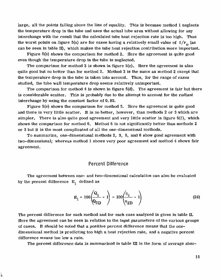
A 13 26.5 4.5 4.712.8 B 11 33.8 5.6 8.4 7.0 C 15 27.9 1.5 6.8 9.2

TABU3 m. - S U M M Y OF DIFFERENCE DATA

3.3 5.6 6.4 4.5 4.7 3.4

Group I Number I Method

Average absolute percent difference

Overall 39

Maximum abs lute percent difference

2.7 1.7 1.4 1.9

lute values of percent difference and the maximum absolute value of percent difference. As in figure 5, it can be seen here that methods 2, 3, 5, and 6 are in good agreement with the two- dimensional method. The best meth- ods, on the average, are 2 and 6, with values of average absolute percent dif- ference of 1.8 and 1.9, respectively. Both methods have a value of 5.6 for the maximum absolute percent differ- ence, which is an indication of the per- formance of a method at its worst. Thus it appears that for the average radiator configurations likely to be

encountered, method 2 will give as close agreement with the two-dimensional as method 6. Method 2 has the advantage of being simpler than method 6.

The heat rejection formula for method 2 (eq. (14)) contains only prescribed quantities except for qin which is a function of hin and Ts/Tin. Curves for qin are readily available in the literature (e. g., ref. 9). Furthermore, Ts/Tin can often be assumed to be zero and only one curve (qin against hin) need be used. On the other hand, the for- mula for method 6 (eq. (18)), contains three quantities not directly prescribed To, q:, and T . The outside tube wall temperature To is calculated by assuming one-dimensional radial heat conduction in a radiating tube. The overall blackbody effectiveness q; is a function of Nc, Q/ro, and Ts/To; Ts/To is often assumed to be zero and is obtained by interpolation from plots of q: against P / ro and Nc (ref. 5). The apparent emissivity T is a function of E , Q/ro, and Ts/T * here Ts/To is assumed to be zero and T is obtained by interpolation from plots of E against Q/ro and E (ref. 5).

Because of its simplicity and accuracy, method 2 is recommended for central fin- tube radiator calculations except for cases with very large ro/ri (say, greater than 4.0). For these latter cases, method 3, which is only slightly more complicated (the temper- ature drop in the tube must be calculated), can be used.

0:

Effect of Input Parameters on Percent Difference

The cases of group B in table 11 were analyzed in order to determine the effect of the independent dimensionless parameters on percent difference. Case B1 is the standard case and its parameters have typical values as obtained in current near-minimum-weight

16

16 1 2 3 .01 .02 .03 0 .4 .a ro'r in til OS

0 1 2 0 a 4 n Llro

Independent dimensionless parameters

Figure 6. -Effect of change in independent dimensionless parameters on percent difference.

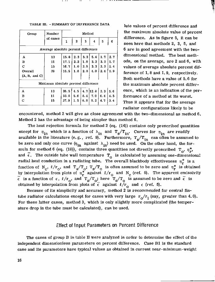
design studies at Lewis. The other cases were obtained by holding all parameters but one constant and taking high and low extreme values spanning the range of current interest. For example, case B1 has a kin of 1.0, case B2 of 0. 5, and case B3 of 2.0 with the other parameters being identical for all three cases. This results in three data points for each parameter. The results are shown in figure 6 for one-dimensional methods 2, 3, 5, and 6. It should be pointed out that the level of the curves (i. e., their location rel- ative to zero percent difference) is the result of the particular set of parameters chosen for the standard case.

In looking at all the parts of figure 6, it can be seen that, in general, variation in Q/ro has the greatest effect (particularly at small Q/ro), variation in t/Q has the next greatest effect, and variation in 8 , has practically no effect. tion is that all four methods exhibit essentially the same trends except for the Q/ro curve for method 6.

Another general observa-

CONCLU SlON S

Results of the two-dimensional analysis of the heat transfer in the cross section of a central fin-tube radiator have been used to evaluate several one-dimensional methods of calculating the heat rejection rate of such radiators. Most of the one-dimensional methods give good agreement with the two-dimensional; however, they a re of varying degrees of complexity. In view of the good agreement of the method (number 2) that neglects tube

17

wall temperature drop and accounts for radiant interchange simply by using the projected area of the tube, it seems unwarranted to use more complicated methods.

Lewis Research Center, National Aeronautics and Space Administration,

Cleveland, Ohio, June 30, 1966, 120-27-04-36 -22.

18

APPENDIX A

SYMBOLS

A

B

a dA*

Ei

F1-2

H

8

k

L

Q

NC

Q

&id q

R

r

S

T

area of radiator surface per unit axial length

radiosity, sum of emitted plus re- flected energy leaving surface per unit time and area

particular element of area

percent difference of method i

view factor, fraction of radiant energy leaving surface 1 that strikes surface 2

total energy incident on a surface per unit time and unit area

thermal conductivity, summation

Qt/Q2 = t/Q

fin half length, see fig. 2

blackbody conductance par am eter , aT:Q '/kt

index (appendix C)

calculated heat rejection rate

ideal heat rejection rate, eq. (20)

energy radiated per unit time and per unit area

rt/Q

radial coordinate in tube

arbitrary surface representing surroundings

temperature

TS

t

X

X

Y

Y

a

E

E -

77

77 in

70

VT

77;

8

x P

U

50

w

equivalent sink temperature

fin half thickness, see fig. 2

xt/Q

horizontal coordinate in fin

Y V Q 2

vertical coordinate in fin

absorptance

emittance

apparent emissivity

overall efficiency

fin efficiency based on Tin

fin efficiency based on To

overall effectiveness, ref. 5

overall effectiveness, refs. 4 and 6

dimensionless temperature, T / T ~ ~

conductance parameter, E uTbQ /kt

reflectance

Stefan- Boltz mann constant

3 2

angular coordinate in tube, see fig. 3

over r elaxation par am eter , appen- dix C

Subscripts :

b fin base

2D based on two-dimensional analysis

i based on one-dimensional method i, i = l , 2 . . . 6

19

I II I I 1.111. I., I. -1.111. I I I 1 . . . . . -

i, j, k

in inside tube wall

L lower limit of visibility

indices, appendix C U upper limit of visibility

1 tube 1 2 tube 2

0 outside tube wall Superscript :

S referring to area of arbitrary sur- m iteration number, appendix C face S

20

APPENDIX B

DERIVATION OF EQUATION FOR lNCl DENT RADIATION

The total radiation Ha* incident on an element dA* of the fin or tube is made up of radiation from other parts of the fin or tube and radiation from the surroundings. In equation form,

where qA-dA* is the heat per unit time leaving all of the fin and tube surface A and striking a unit area of dA*, and qs-dA* is the heat per unit time leaving the surround- ings o r sink which may be represented by an arbitrary surface S (fig. 7) and striking a unit area of dA*. The q's are given by

and

QS-dA* dA*

CIS-&* =

where QA-dA * is the heat per unit time leaving all of A and striking all of dA*, and

Qs is that leaving all of S and striking all of dA*. The Q's a r e given by

and

where BdA is the radiosity, that is, the total energy emitted plus reflected leaving dA per unit time, dFdA - dA* is the view factor from dA to dA*, Ts is the equivalent sink temperature of the surroundings, S is the area of surface S, and dFS-dA* is the view

21

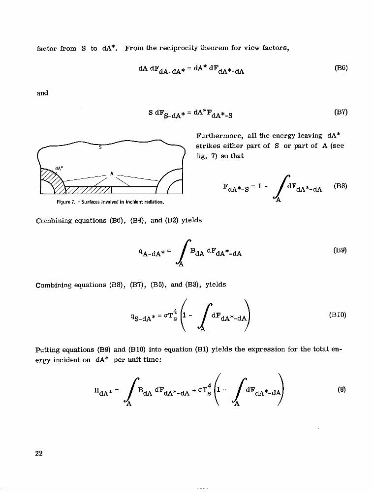
factor from S to dA*. From the reciprocity theorem for view factors,

dA dFdA,dA* = dA* dFdA*,dA

and

Furthermore, all the energy leaving dA* strikes either part of S or part of A (see fig. 7) so that

Figure 7. - Surfaces involved i n incident radiation. c/A

Combining equations (B6), (B4), and (B2) yields

Combining equations (B8), (B7), (B5), and (B3), yields

Putting equations (B9) and (B10) into equation (Bl) yields the expression for the total en- ergy incident on dA* per unit time:

22

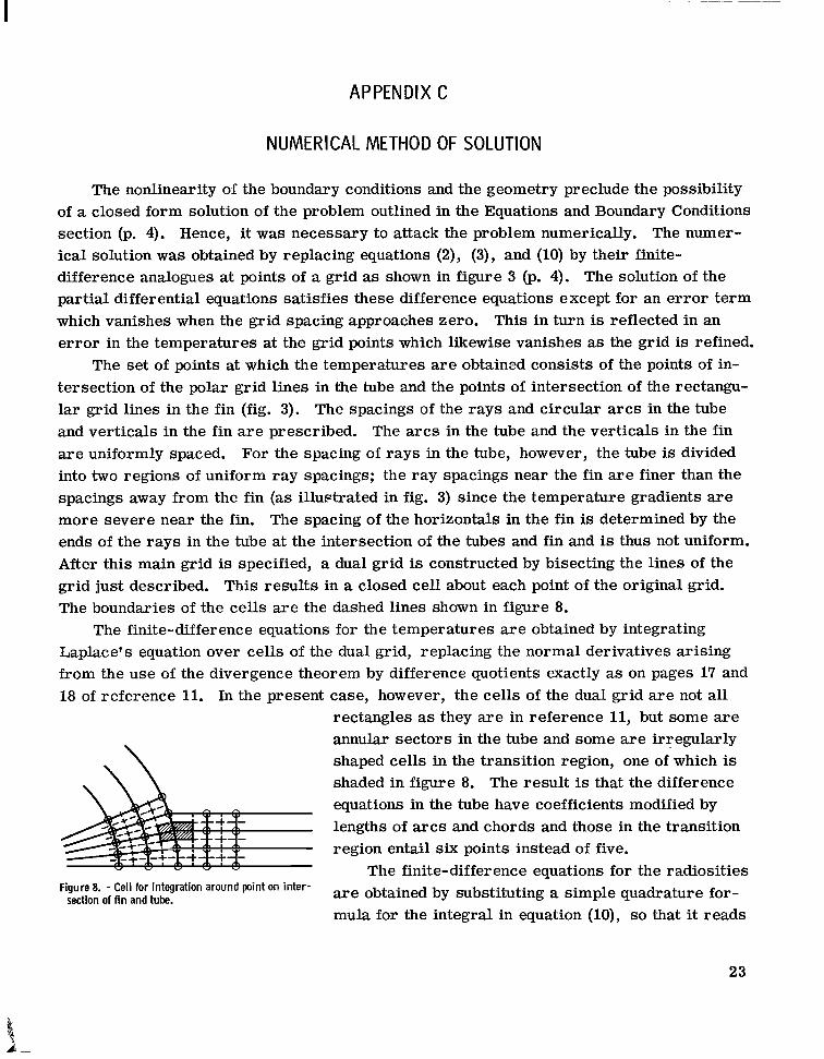
APPENDIX C

NUMERICAL METHOD OF SOLUTION

The nonlinearity of the boundary conditions and the geometry preclude the possibility

The numer- of a closed form solution of the problem outlined in the Equations and Boundary Conditions section (p. 4). Hence, it was necessary to attack the problem numerically. ical solution was obtained by replacing equations (2), (3), and (10) by their finite- difference analogues at points of a grid as shown in figure 3 (p. 4). The solution of the partial differential equations satisfies these difference equations except for an e r ror term which vanishes when the grid spacing approaches zero. This in turn is reflected in an error in the temperatures at the grid points which likewise vanishes as the grid is refined.

tersection of the polar grid lines in the tube and the points of intersection of the rectangu- lar grid lines in the fin (fig. 3). The spacings of the rays and circular arcs in the tube and verticals in the fin a re prescribed. The a rcs in the tube and the verticals in the fin a re uniformly spaced. For the spacing of rays in the tube, however, the tube is divided into two regions of uniform ray spacings; the ray spacings near the fin are finer than the spacings away from the fin (as illustrated in fig. 3) since the temperature gradients are more severe near the fin. The spacing of the horizontals in the fin is determined by the ends of the rays in the tube at the intersection of the tubes and fin and is thus not uniform. After this main grid is specified, a dual grid is constructed by bisecting the lines of the grid just described. The boundaries of the cells are the dashed lines shown in figure 8.

The finite-difference equations for the temperatures a re obtained by integrating Laplace's equation over cells of the dual grid, replacing the normal derivatives arising from the use of the divergence theorem by difference quotients exactly as on pages 17 and 18 of reference 11. In the present case, however, the cells of the dual grid a re not all

The set of points at which the temperatures are obtained consists of the points of in-

This results in a closed cell about each point of the original grid.

rectangles as they are in reference 11, but some are annular sectors in the tube and some are irregularly shaped cells in the transition region, one of which is shaded in figure 8. The result is that the difference equations in the tube have coefficients modified by lengths of a rcs and chords and those in the transition region entail six points instead of five.

The finite-difference equations for the radiosities are obtained by substituting a simple quadrature for- mula for the integral in equation (lo), so that it reads

Figure 8. - Cell for integration around point on inter- section of fin and tube.

23

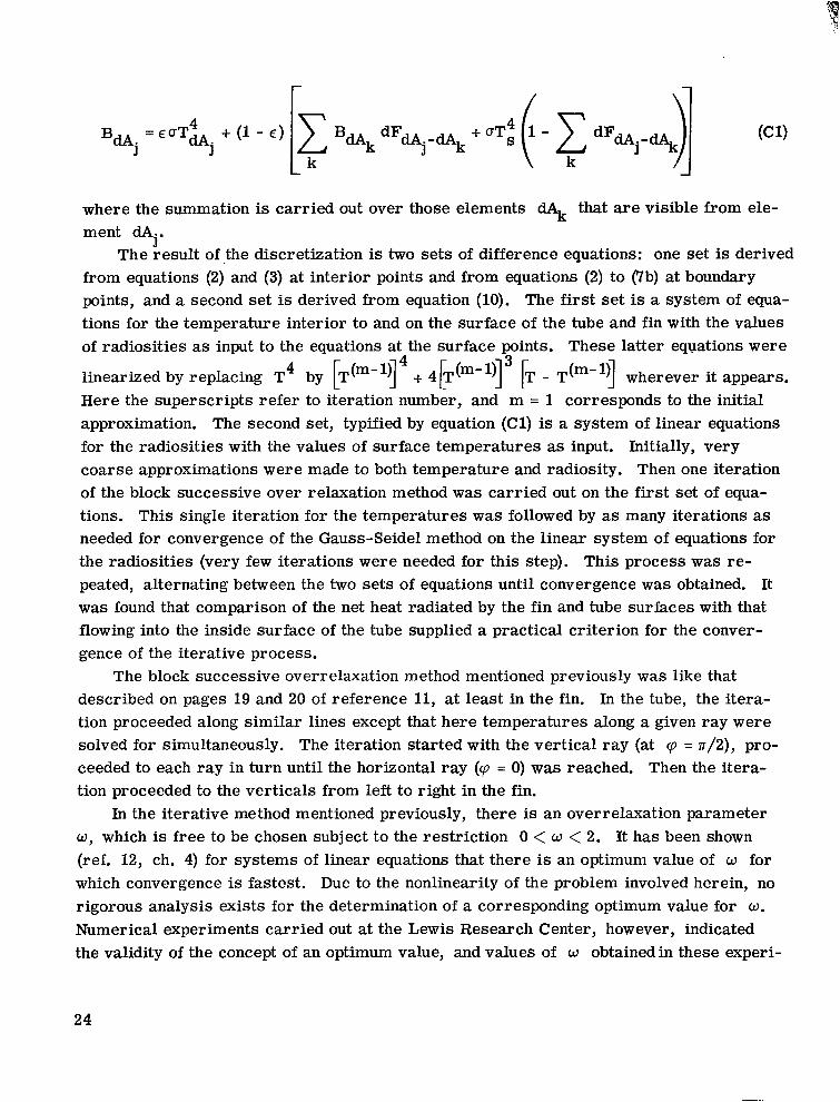
where the summation is carried out over those elements dAk that are visible from ele- ment dA

The result of the discretization is two sets of difference equations: one set is derived from equations (2) and (3) at interior points and from equations (2) to (7b) at boundary points, and a second set is derived from equation (10). The first set is a system of equa- tions for the temperature interior to and on the surface of the tube and fin with the values

j*

of radiosities as input to the equations at the surface points. These latter equations were

linearized by replacing T4 by [T(m-l)I + 4b(m-1)l - T(m-l)I wherever it appears. 4 3

Here the superscripts refer to iteration number, and m = 1 corresponds to the initial approximation. The second set, typified by equation (Cl) is a system of linear equations for the radiosities with the values of surface temperatures as input. Initially, very coarse approximations were made to both temperature and radiosity. Then one iteration of the block successive over relaxation method was carried out on the first set of equa- tions. This single iteration for the temperatures was followed by as many iterations as needed for convergence of the Gauss-Seidel method on the linear system of equations for the radiosities (very few iterations were needed for this step). This process was re- peated, alternating between the two sets of equations until convergence was obtained. It was found that comparison of the net heat radiated by the fin and tube surfaces with that flowing into the inside surface of the tube supplied a practical criterion for the conver- gence of the iterative process.

The block successive overrelaxation method mentioned previously was like that described on pages 19 and 20 of reference 11, at least in the fin. In the tube, the itera- tion proceeded along similar lines except that here temperatures along a given ray were solved for simultaneously. The iteration started with the vertical ray (at q = 7~/2), pro- ceeded to each ray in turn until the horizontal ray (q = 0) was reached. Then the itera- tion proceeded to the verticals from left to right in the fin.

In the iterative method mentioned previously, there is an overrelaxation parameter w, which is free to be chosen subject to the restriction 0 < w < 2. It has been shown (ref. 12, ch. 4) for systems of linear equations that there is an optimum value of w for which convergence is fastest. Due to the nonlinearity of the problem involved herein, no rigorous analysis exists for the determination of a corresponding optimum value for w. Numerical experiments carried out at the Lewis Research Center, however, indicated the validity of the concept of an optimum value, and values of w obtainedin these experi-

24

ments were used for the production runs. A typical result is w = 1.93 for 690 points leading to convergence of the relative error in the heat balance to less than 1.0 percent in 180 iterations.

25

L

I .... ,.I-

APPENDIX D

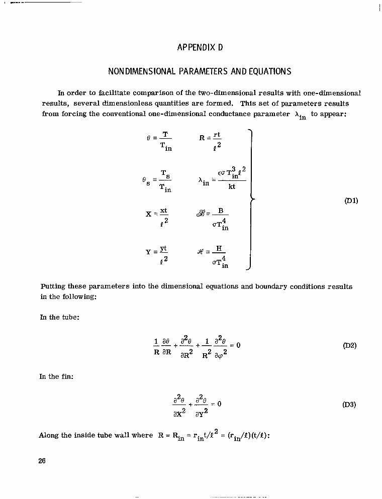
NONDIMENSIONAL PARAMETERS AND EQUATIONS

In order to facilitate comparison of the two-dimensional results with one-dimensional results, several dimensionless quantities are formed. This set of parameters results from forcing the conventional one-dimensional conductance parameter hin to appear:

3 2 EU TinQ

kt - e =- TS Xin =

S T:, 111

f

Putting these parameters into the dimensional equations and boundary conditions results in the following:

In the tube:

1 ae a2e +--=o 1 a2e -- +-

In the fin:

& a20 +- = 0 ax2 ay2

2 Along the inside tube wall where R = Rin = rint/Q = (rin/Q)(t/Q):

26

8(Rin, cp) = 1.0

Along cp = 0 and cp = s /2 in the tube:

Along Y = 0 and X = (Q + ro)t/Q2 = (1 + ro/J?)t/Q:

(E) =(E) = o a y y=o ax X=(l+ro/Q)t/Q

On the surface of the tube where R = R, = r0t/t2 = (ro/f)(t/Q):

2 2. On the surface of the fin where Y = t /Q .

where

034)

03 5)

Thus, it can be seen that the dimensionless temperature 8 depends on the parameters Xin, rin/f, ro/Q, t/Q, Os, and E . In this report, E will always be fixed at 0.9 and can

27

be eliminated from the list of variables. Of the remaining parameters, hin, ro/Q (often written Q/ro), and 8, are the commonly used one-dimensional parameters and rin/Q and t/Q are two-dimensional parameters. Instead of rin/Q, it is more informative to use ro/rin, which is the ratio of ro/Q to rin/Q. To summarize, in this report the parameters determining the two-dimensional heat transfer in a fin-tube radiator are hin,

ro/Q (or Q/ro), os, ro/rin, and t/Q.

28

I

REFER EN C E S

1. Schreiber, L. H.; Mitchell, R. P.; Gillespie, G. D.; andolcott, R. M.: Tech- niques for Optimization of a Finned-Tube Radiator. Paper No. 61-SA-44, ASME, June 196 1.

2. Callinan, Joseph P. ; and Berggren, Willard P. : Some Radiator Design Criteria for Space Vehicles. J. Heat Transfer, vol. 81, no. 3, Aug. 1959, pp. 237-244.

3. Mackay, D. B. ; and Bacha, C. P. : Space Radiator Analysis and Design. Part I. Rep. No. SID 61-66 (AFASD TR 61-30, pt. l), North American Aviation, Inc., Apr. 1, 1961, pp. 11-22.

4. Haller, Henry C. ; Wesling, Gordon C. ; and Lieblein, Seymour: Heat-Rejection and Weight Characteristics of Fin-Tube Space Radiators with Tapered Fins. NASA TN D-2168, 1964.

5. Krebs, Richard P. ; Haller, Henry C. ; and Auer, Bruce M. : Analysis and Design Procedures for a Flat, Direct-Condensing, Central Finned-Tube Radiator. NASA TN D-2474, 1964.

6. Saule, Arthur V. ; Krebs, Richard P. ; and Auer, Bruce M. : Design Analysis and General Characteristics of Flat-Plate Central- Fin-Tube Sensible-Heat Space Radi- ators. NASA TN D-2839, 1965.

7. Sparrow, E. M. ; and Eckert, E. R. G. : Radiant Interaction Between Fin and Base Surfaces. J. Heat Transfer, vol. 84, no. 1, Feb. 1962, pp. 12-18.

8. Krebs, Richard P. ; Winch, David M. ; and Lieblein, Seymour: Analysis of a Mega- watt Level Direct Condenser-Radiator. Power Systems for Space Flight. Vol. 11 of Progress in Astronautics and Aeronautics, Morris Zipkin and Russell N. Edwards, eds. , Academic Press, Inc., 1963, pp. 475-504.

9. Lieblein, Seymour: Analysis of Temperature Distribution and Radiant Heat Transfer Along a Rectangular Fin of Constant Thickness. NASA TN D-196, 1959.

10. Sotos, Carol J. ; and Stockman, Norbert 0. : Radiant-Interchange View Factors and Limits of Visibility for Differential Cylindrical Surfaces with Parallel Generating Lines. NASA TN D-2556, 1964.

11. Stockman, Norbert 0. ; and Bittner, Edward C. : Two-Dimensional Heat Transfer in Radiating Stainless-Steel-Clad Copper Fins. NASA T N D-3102, 1965.

12. Varga, R. S. : Matrix Iterative Analysis. Prentice-Hall, Inc., 1962.

NASA-Langley, 1966 E-3346 29

“The aeronautical and space activities of the United States shall be conducted so as to contribute . . . to the expansion of human knowl- edge of phenomena in the atmosphere and space. The Administration shall provide for the widest practicable and appropriate dissemination of information concerning its activities and the results thereof .”

-NATIONAL AERONAUTICS AND SPACE ACT OF 1958

NASA SCIENTIFIC AND TECHNICAL PUBLICATIONS

TECHNICAL REPORTS: important, complete, and a lasting contribution to existing knowledge.

TECHNICAL NOTES: of importance as a contribution to existing knowledge.

TECHNICAL MEMORANDUMS: Information receiving limited distri- bution because of preliminary data, security classification, or other reasons.

CONTRACTOR REPORTS: Technical information generated in con- nection with a NASA contract or grant and released under NASA auspices,

TECHNICAL TRANSLATIONS: , Information published in a foreign language considered to merit NASA distribution in English.

TECHNICAL REPRINTS: Information derived from NASA activities and initially published in the form of journal articles.

SPECIAL PUBLICATIONS: Information derived from or of value to NASA activities but not necessarily reporting the results .of individual NASA-programmed scientific efforts. Publications include conference proceedings, monographs, data compilations, handbooks, sourcebooks, and special bibliographies.

Scientific and technical information considered

Information less broad in scope but nevertheless

Details on the availability of these publications may be obtained from:

SCIENTIFIC AND TECHNICAL INFORMATION DIVISION

NATIONAL AERONAUTICS AND SPACE ADMINISTRATION

Washington, D.C. PO546