Comparison of NOAA’s Operational AVHRR Derived Cloud...

Comparison of NOAA's Operational AVHRR DerivedCloud Amount to other Satellite Derived Cloud

Climatologies.

Sarah M. Thomas University of Wisconsin, Cooperative Institute for Meteorological Satellite

Studies (CIMSS)

Andrew K. HeidingerNOAA/NESDIS Office of Research and Applications

Michael J. PavolonisUniversity of Wisconsin, Cooperative Institute for Meteorological Satellite

Studies (CIMSS)

Submitted to: Journal of Climate

Date Submitted: 11/05/2003

Date Revised: 05/04/2004

Date Accepted:

Abstract

A comparison is made between a new operational NOAA AVHRR global cloud

amount product to those from established satellite-derived cloud climatologies. The new

operational NOAA AVHRR cloud amount is derived using the cloud detection scheme in the

extended Clouds from AVHRR (CLAVR-x) system. The cloud mask within CLAVR-x is a

replacement for the CLAVR-1 cloud mask. Previous analysis of the CLAVR-1 cloud

climatologies reveals that its utility for climate studies is reduced by poor high latitude

performance and inability to include data from the morning orbiting satellites. This study

demonstrates, through comparison with established satellite-derived cloud climatologies, the

ability of CLAVR-x to overcome the two main shortcomings of the CLAVR-1 derived cloud

climatologies. While systematic differences remain in the cloud amounts from CLAVR-x and

other climatologies, no evidence is seen that these differences represent a failure of the CLAVR-

x cloud detection scheme. Comparisons for July 1995 and January 1996 indicate that for most

latitude zones, CLAVR-x produces less cloud than ISCCP and UW/HIRS. Comparisons to

MODIS for April 1-8, 2003 also reveal that CLAVR-x tends to produce less cloud. Comparison

of the seasonal cycle (July-January) of cloud difference with ISCCP, however, indicates close

agreement. It is argued that these differences may be due to the methodology used to construct a

cloud amount from the individual pixel level cloud detection results. Overall, the global cloud

amounts from CLAVR-x appear to be an improvement over those from CLAVR-1 and compare

well to those from established satellite cloud climatologies. The CLAVR-x cloud detection

results have been operational since late 2003, and are available in real-time from NOAA.

1

1. Introduction

Cloud radiative effects play a central role in the Earth's climate system (Liou 1986;

Ramanathan et al. 1989; Rossow and Lacis 1990; Stephens and Greenwald 1991) . Cloud cover

is a key factor in determining the magnitude of the exchange of incoming solar energy and

outgoing terrestrial energy (Pavolonis and Key, 2003); an exchange that is central to

understanding the natural fluctuations in the Earth's climate system. Hence, an accurate

determination of the global extent of cloud cover is imperative for studies of the Earth's climate.

As satellite imagers continue to become more advanced, there are an increasing number of

opportunities to study the Earth's atmospheric, biological, and geophysical processes, as well as

land and ocean surface properties in great detail. However, many of these studies, such as

retrievals of aerosol optical properties and surface temperature, or studies of snow and sea ice

extent, rely on clear sky radiances in the data reduction process. Even small amounts of cloud

contamination in a scene can dramatically change the radiative properties derived using satellite

measurements.

Although cloud amount is a fundamental quantity, satellite derived estimates of it

vary significantly. Trends in cloud amount from a variety of studies have even shown regional

trends of differing sign. For example, the decrease in tropical cloud amount evident in the

ISCCP (International Satellite Cloud Climatology Project) products during the 1990s (Wielicki

et al., 2002) is not present in the UW-HIRS (University of Wisconsin High resolution Infrared

Radiation Sounder) cloud climatology (Wylie and Menzel, 1999). For these reasons, a great deal

of effort has been focused on developing algorithms that use satellite radiometric data in a

2

temporally consistent manner to detect clouds accurately on a global scale.

One instrument that provides data useful for these types of studies is the National

Oceanic and Atmospheric Administration (NOAA) Advanced Very High Resolution Radiometer

(AVHRR). The purpose of this study is to examine the performance of the extended Clouds

from AVHRR (CLAVR-x) cloud detection algorithm over a range of seasonal conditions and

satellite equator crossing times. This will be accomplished through comparisons with cloud

amounts from ISCCP, Clouds from AVHRR phase 1 (CLAVR-1), Moderate resolution Imaging

Spectroradiometer (MODIS), AVHRR Polar Pathfinder (APP), and UW-HIRS. Characteristics

of the global cloud distribution from CLAVR-x relative to other cloud products will be

presented. Of primary importance is the question of whether or not CLAVR-x provides results

that are consistent with other estimates of the global cloud distribution, while offering

improvements over previous cloud detection algorithms that use AVHRR data.

A detailed description of each of the cloud detection algorithms used for

comparison is given in section 2. In section 3, global cloud amounts from CLAVR-x are

compared to the results from the other aforementioned cloud climatologies. Several examples

are given that highlight the key similarities and differences between CLAVR-x and each of the

other products, for a variety of satellite equator crossing times and seasonal conditions. Potential

strengths and/or shortcomings of CLAVR-x are discussed in this section. Section 4 summarizes

the results from this study.

3

2. Overview of Cloud Amount Algorithms

Satellite imagers have the ability to assess global cloud properties on much finer

spatial and temporal scales than any other type of instrument currently available. Hence, many

efforts have been made over the past 25 years to develop accurate methods by which data from

satellite imagers may be used not only to detect clouds, but also to document the global extent of

cloud occurrence and properties.

a. ISCCP Cloud Amount Algorithm

One of the first large scale, organized attempts to use satellite data to create a global

cloud climatology was ISCCP, which was established in 1982. An overview of the ISCCP

program is given by Schiffer and Rossow (1983). Radiance data from geostationary satellites

such as GOES (Geostationary Operational Environmental Satellite), METEOSAT (geostationary

Meteorological Satellite), and GMS (Geostationary Meteorological Satellite) are averaged over 3

hr intervals to provide complete coverage of the tropics and mid-latitudes at a high temporal

resolution. Global coverage is attained by using AVHRR data from a suite of NOAA polar-

orbiting satellites to provide measurements poleward of 60 N/S. ISCCP pixels are mapped to a

250 km equal area grid, and as described by Schiffer and Rossow (1983), variations over this

area are small compared to time variations. The ISCCP data record spans from 1983-2002, and

is the longest and most complete satellite derived cloud climatology currently available.

A complete description of the ISCCP cloud amount algorithm is given by Rossow

and Garder (1993). ISCCP clear/cloudy classification is based largely on the analysis of spatial

and temporal variability in reflectance and/or brightness temperature (BT) over a geographically

4

small region. These uniformity tests are based on the assertion that clear pixels tend to exhibit

less variability in both space and time than do cloudy pixels (McClain et al. 1985). For a pixel to

be classified as cloudy, it must have a BT much colder than the warmest pixel in a small spatial

domain. In addition, the pixel must exhibit significant variability in BT over a period of 3

consecutive days. A pixel is classified as cloudy only if it meets both the spatial and temporal

variability requirements. In addition, clear sky statistics are compiled once every 5 days using

both IR and VIS data. These statistics are used to enhance the cloud mask by providing

additional threshold values by which pixels may be classified as clear or cloudy (e.g. A pixel is

cloudy if it is colder than the 5-day statistical mean clear-sky BT, or has a higher VIS reflectance

than the statistical mean clear-sky reflectance.) After all pixels have been classified, total cloud

fraction is calculated for each 250 km grid cell by taking the ratio of the number of cloudy pixels

to the total number of pixels. This calculation carries the assumption that there are no partially

cloud filled pixels, and every cloudy pixel is 100% cloud covered.

b. CLAVR-1 Cloud Amount Algorithm

The ISCCP cloud amount algorithm uses IR and VIS data from AVHRR in order to

attain measurements over polar regions and achieve global coverage. However, AVHRR has

cloud detection capabilities beyond the two channel methods used by ISCCP. Utilization of all

the spectral information provided by AVHRR was one motivating factor for the development of

an AVHRR-only cloud mask by NOAA, and resulted in the creation of the CLAVR-1 cloud

mask (Stowe et al., 1999). AVHRR data from satellites prior to NOAA-15 provide radiances

over 5 wavelength bands with central wavelengths of 0.63, 0.86, 3.75, 10.8, and 12 µm.

5

AVHRR data from after the launch of NOAA-15 provide observations over an additional band

with a central wavelength of 1.6 µm, however cannot simultaneously provide observations from

the 3.75 µm channel. AVHRR has a spatial resolution of 1 km, but these data are available over

limited areas. The Global Area Coverage (GAC) AVHRR data are used for this study, and have

a spatial resolution of 4 km at nadir. The traditional 5 channel AVHRR data record encompasses

over 23 years of data (1981-2004). The AVHRR data record is scheduled to continue until 2018,

through the European organization for the exploitation of meteorological satellites

(EUMETSAT) polar-orbiting operational meteorological satellites (MetOp) program. This gives

AVHRR the potential to be very valuable for use in climate studies, including studies of global

cloud distribution and physical properties.

The CLAVR-1 cloud detection algorithm is a pixel level cloud mask that uses all of

the spectral information that AVHRR provides. It was developed for use in multiple NESDIS

(National Environmental Satellite Data and Information Service) products, and its heritage lies in

the NESDIS operational sea surface temperature algorithm (McClain, 1989). A detailed

description of the CLAVR-1 cloud mask is provided by Stowe et al. (1999). CLAVR-1

implements three primary types of tests in order to determine whether a pixel is clear or cloudy:

contrast signature tests, spectral signature tests, and spatial signature tests. The contrast

signature tests require that for each pixel, the reflectance or BT for a single AVHRR band be

compared against a fixed threshold value that separates clear and cloudy conditions. The

threshold used for each test is adjusted based on the surface type (e.g. vegetated land, ocean,

desert... etc.) of the scene. The spectral signature tests involve the combination of multiple

6

AVHRR bands. These tests compare either the ratio or difference of two bands against a

clear/cloudy threshold value. Finally, a spatial uniformity test is implemented. Similar to

ISCCP, this test operates on the assumption that over small spatial areas (in the case of CLAVR-

1, a 2x2 pixel array), cloud free scenes are relatively uniform in their reflectance and BT. Based

on the results of the aforementioned tests, a pixel is classified into one of three categories: clear,

mixed, or cloudy. Cloud fraction, f(c), is calculated based on the assumption that cloudy scenes

are 100% cloudy, mixed scenes are 50% cloudy, and clear scenes are 0% cloudy, using the

following expression:

(1) f(c) = Ncloudy + 0.5*Nmixed

Ntotal

Where Ncloudy is the number of cloudy pixels, Nmixed is the number of mixed pixels, and Ntotal is the

total number of pixels in the scene.

c. CLAVR-x Cloud Amount Algorithm

Further development of CLAVR-1 has led to the extended CLAVR algorithm

(CLAVR-x). CLAVR-x became an operational product in late 2003, and the CLAVR-x cloud

detection results are currently available in the space alloted in the NOAA AVHRR 1b format.

CLAVR-x is based on the same physical principles as CLAVR-1. However, numerous updates

have been made in order to improve upon some of the documented shortcomings of CLAVR-1.

An algorithm theoretical basis document (ATBD) is available on-line for CLAVR-x, which fully

describes the cloud amount algorithm (Heidinger, 2004). In addition, parts of the CLAVR-x

cloud mask are described by Heidinger et al. 2002, and Heidinger et al. 2004. One of the major

7

improvements of CLAVR-x over CLAVR-1 is the breakdown of the mixed category into two

new categories: mixed-cloudy and mixed-clear. Mixed cloudy pixels are those pixels that are

determined to be cloudy by one or more of the contrast or spectral signature tests, but are

spatially non-uniform as determined by uniformity tests. Likewise, mixed-clear pixels are those

pixels that are determined to be clear but are spatially non-uniform . The mixed category is

divided into two sub-categories to improve the accuracy of the total cloud fraction calculation by

allowing more realistic percent cloud cover values be assigned to mixed pixels. CLAVR-x cloud

fraction is calculated based on the assumption that cloudy scenes are 100% cloudy, mixed-

cloudy scenes are 88% cloudy, mixed-clear scenes are 13% cloudy, and clear scenes are 0%

cloudy. These percentages are derived by analyzing the mean radiances from grid-cells that

report both clear and cloudy pixels. A radiometric balance approach similar to the one described

in Molnar and Coakley (1985) is used to estimate the cloud fraction of the partly clear and the

partly cloudy pixels. This approach calculates the radiance for a partly clear/cloudy pixel

assuming that it is a linear function of the fully cloudy and fully clear radiances. Cloud fraction

is then derived using the following expression:

(2) f(c) = Imixed-cloudy-Iclear Icloudy-Iclear

Where Imixed-cloudy is the mixed-cloudy radiance, Icloudy is the fully cloudy radiance, and Iclear is the

clear sky radiance. This radiometric balance approach is applied to the mean 11 µm radiances

derived from the clear, partly clear, partly cloudy, and cloudy pixels. Only pixels with valid

clear and cloudy radiances are used. Figure 1 shows the distribution of these cloud fractions for

the partly clear and partly cloudy pixels from one day of data from June 1995. In this figure, the

8

partly cloudy results are shown separately for ice and water clouds and the mean cloud amounts

for each distribution are given in the figure legend. Occasionally, the radiance for a partly

cloudy pixel will exceed the radiance for a fully cloudy pixel, which leads to the cloud fraction

weight being greater than 1. Similarly, sometimes the radiance of a partly clear pixel will be

lower than that of a fully clear pixel, which results in the cloud fraction weight being less than 0.

These occurrences, however, are rare and do not affect the final cloud fractions assigned. The

semi-transparent nature of partly cloudy ice pixels is the likely cause of the decrease in the partly

cloudy ice fraction relative to the partly cloudy water cloud fraction. Because the radiometric

balance approximation assumes clouds are opaque and this assumption is most valid for water

clouds, the partly cloudy fraction computed for water clouds will be used for all clouds. For the

rest of the study, the cloud fraction weights of the mixed-clear and mixed-cloudy pixels are 13%

and 88%, respectively. Using these fixed values, CLAVR-x cloud fraction, f(c), is calculated

using the following expression:

(3) f(c) = Ncloudy + 0.88*Nmixed-cloudy + 0.13*Nmixed-clear

Ntotal

where Ncloudy is the number of cloudy pixels, Nmixed-cloudy is the number of mixed-cloudy pixels,

Nmixed-clear is the number of mixed-clear pixels,and Ntotal is the total number of pixels in the scene.

Another key development in CLAVR-x is the more accurate detection of clouds in

polar regions and regions of snow or sea-ice cover. This involves not only the modification of

cloud mask thresholds in regions with snow or ice, but also the improvement of the snow and ice

detection algorithm itself. The threshold modifications are based largely on the previous

methods of the AVHRR Polar Pathfinder (APP) cloud mask (Key and Barry, 1989), which will

9

be described later. This cloud mask contains developments specifically designed for use

poleward of 45o N or S. The CLAVR-x cloud mask procedures in the high latitudes are based on

the APP methods when possible. However, APP also employs temporal tests in its cloud mask

determination that are absent in CLAVR-x. The difference between CLAVR-x and APP will in

some part be an indication of the relative impact of the APP temporal tests. Similar to APP,

CLAVR-x includes a tighter range of values for the 3.75-12 µm test (TMFT), and a lower

threshold value for the 11 – 12 µm test (FMFT) than did CLAVR-1. These threshold

modifications lead to an overall lower cloud fraction in polar regions than produced by CLAVR-

1. This lower cloud fraction is in better agreement with other cloud climatologies.

In addition to modified thresholds for polar regions, CLAVR-x includes a revised

algorithm for the detection of snow and ice. This algorithm employs the use of the Normalized

Difference Snow Index (NDSI), developed for use with MODIS Snowmap (Hall and

Salomonson, 2001), for scenes where AVHRR channel 3a (1.64 µm) is available. In all other

cases, a grouped threshold approach similar to that described by Baum et al. (1999) is used. This

approach makes use of the characteristic low reflectance of snow at 3.75 µm, and the low BTD

(3.75 – 11 µm) as compared to clouds. Since clouds and snow typically share similar spectral

properties such as high reflectance at 0.65 µm and a low 11 µm BT, improved methods of

distinguishing between clouds and snow leads to a more accurate calculation of cloud fraction in

polar regions.

As noted by Stowe et al. (1999), the CLAVR-1 cloud detection algorithm should be

applied only to data from satellites with afternoon equator crossing times. This is due to the fact

10

that CLAVR-1 is not seasoned at detecting clouds in regions where the solar zenith angle is high.

Therefore, since satellites that cross the equator in the morning (such as NOAA-12) tend to view

much of the globe around dawn (when the solar zenith angle is high), CLAVR-1 can not be

reliably applied to data from these satellites. Where CLAVR-1 uses single value thresholds for

the reflectance tests, CLAVR-x adopts reflectance tests that have a dependence on the solar and

satellite viewing geometry. These modifications to CLAVR-x appear to have extended the

applicability of the CLAVR-x cloud detection to all orbits. As will be discussed later, the

CLAVR-x total cloud amounts behave similarly in the morning and the afternoon orbits,

allowing for a more true estimate of the diurnal average.

d. MODIS Cloud Amount Algorithm

Advancement in satellite imager technology has made more rigorous cloud

detection algorithms involving multi-spectral techniques possible. The Moderate Resolution

Imaging Spectroradiometer (MODIS) was launched aboard the NASA Earth Observing System

(EOS) Terra platform in 1998 and Aqua platform in 2002. A complete description of the

MODIS instrument is given by Salomonson et al. (1989). This focus of this study is on cloud

amounts derived from MODIS-Terra data rather than MODIS-Aqua data, because the orbit of the

Terra platform is closer to that of NOAA-16. The Terra platform has a polar-orbiting, sun-

synchronous orbit. MODIS has a total of 36 spectral bands between 0.415 and 14.235 µm.

Spatial resolutions for this instrument are 250 m (1 VIS, 1 NIR band), 500 m (2 VIS, 3 NIR

bands), and 1000 m (29 total VIS, NIR and IR bands). The high spatial resolution and large

number of spectral bands available with this instrument make it an excellent tool for studying the

11

intricacies of the Earth's land, ocean, atmosphere, and biological and geophysical processes.

However, the MODIS data record covers only 2000-present, so it has limited use for climate

applications.

A complete description of the MODIS cloud mask is given by Ackerman et al.

(1998). Most cloud detection with the MODIS cloud mask occurs using pixel level spectral

tests. Similar to the CLAVR cloud masks, the MODIS cloud mask classification of a pixel as

clear or cloudy depends on the results from a series of fixed threshold tests. The main difference

between MODIS and CLAVR-x is the availability of specific channels on MODIS that greatly

improve cloud detection in certain regions. For example, channels in the 1.38 and 7.7 µm water

vapor absorption bands greatly improve the detection of thin cirrus (during the day) and clouds

in the polar regions. In addition, CLAVR-x uses spatial uniformity and background fields of

climatological sea surface temperature and vegetation condition to a much greater extent than

MODIS. Similar to CLAVR-x the MODIS cloud mask classifies each pixel into four categories:

confident clear, probably clear, probably cloudy, and confident cloudy. However, unlike

CLAVR-x, the occurrence of two intermediate classes is relatively rare (<10%). In addition,

when a cloud amount is computed from the MODIS cloud mask, the four level mask is converted

to a binary mask, with the clear and probably clear pixels having an assumed zero cloud amount,

and the probably cloudy and confident cloudy having an assumed 100% cloud amount.

e. UW/HIRS Cloud Amount Algorithm

In addition to those studies that use satellite imager data, some studies make use of

the cloud detection capabilities of high spectral resolution, low spatial resolution satellite

12

sounding instruments. UW-HIRS is one such sounder-derived cloud climatology, and spans

from mid-1989 to the present. The High Resolution Infrared Sounder (HIRS) has flown aboard

the NOAA polar-orbiting satellite platforms since its inception in 1978. It senses infrared

radiation in 18 spectral bands between 3.9 and 15 µm, with a spatial resolution of 18.9 km at

nadir. Fields of view are determined to be clear or cloudy by an examination of the 11.2 µm BT.

If the 11.2 µm BT (corrected for moisture absorption) is within 2K of the surface temperature

(taken from hourly surface observation data where available, or if surface data is unavailable, the

surface temperature is assumed to be the warmest temperature across a small geographic area),

then the scene is classified as clear. In addition, the UW-HIRS cloud climatology implements a

CO2 slicing technique aimed at the detection of high clouds (Wylie and Menzel, 1989). This

approach exploits the differences in weighting function for three different CO2 absorption bands

(14.2 µm, 14.0 µm, and 13.3 µm), and is especially skillful at detecting high, thin clouds often

missed by other tests. Similar to other cloud masks discussed, the UW-HIRS cloud mask does

not estimate fractional cloud cover in a single field of view, and thus cloud amount is calculated

by dividing the number of cloudy pixels by the total number of pixels.

f. APP Cloud Amount Algorithm

The AVHRR Polar Pathfinder (APP) cloud mask (Key and Barry, 1989; Key 2002)

uses tests similar to those in CLAVR-x to detect cloud using AVHRR data. However, unlike

CLAVR-x, the tests implemented by APP have been specifically tuned for application to high

latitudes and are available poleward of 45oN and 45oS only. The APP data is AVHRR GAC data

mapped to a 5 km resolution polar stereographic grid and is produced twice daily. A

13

combination of spectral and temporal uniformity tests are used to make a final clear or cloudy

determination. No sub-pixel cloud fraction is estimated. Therefore, cloud amount is derived by

dividing the number of cloudy pixels by the total number of pixels in a scene.

Numerous studies have been conducted to validate APP products in the polar

regions (Wang and Key, 2004; Pavolonis and Key, 2003; Wang and Key, 2003; Key et al. 2001;

Maslanik et al. 2001). These studies have compared results from APP against ISCCP cloud

properties as well as surface observations from the First ISCCP Regional Experiment – Arctic

Cloud Experiment (FIRE-ACE) and Surface Heat Budget of the Arctic Ocean (SHEBA), and

observations from meteorological stations throughout the Arctic and Antarctic. These studies

have shown APP products to be consistent, in many cases, with ground based observations,

although some discrepancies still exist in cases with high, optically thin clouds (Maslanik, et al.,

2001). Wang and Key (2004) show that in the Arctic, APP cloud fraction is more consistent

with ground based observations than is ISCCP, especially during the summer months. Studies

showing a direct comparison between APP and ISCCP cloud fraction over the Antarctic have yet

to be published. However, Pavolonis and Key (2003) indicate that APP derived cloud forcing in

the Antarctic shows better agreement with ground based observations than ISCCP derived cloud

forcing, which can be directly linked to ISCCP under-detection of clouds over snow during the

summer months. Based on the results from these previous studies, this study will assume the

APP cloud amount to be the closest representation to the actual cloud amount in the high

latitudes.

14

3. Data and Methods

This study provides cloud amount comparisons for the months of July 1995,

January 1996, and part of April 2003. A summary of the different types of comparisons made, as

well as the cloud masks used and spatial resolution of each comparison is provided in Table 1. A

range of months is included to provide comparisons from several different seasonal conditions.

The CLAVR-x cloud mask is applied to AVHRR level 1b radiance data from NOAA-12,

NOAA-14, and NOAA-16. The approximate daytime equator crossing time for each of these

satellites is listed in Table 2. Since each of these satellites is in a sun-synchronous orbit, the

nighttime equator crossing time for each satellite is 12 hours after the daytime equator crossing

time. This variety of satellites is used to illustrate the utility of the CLAVR-x cloud mask as

applied to data from both morning and afternoon satellites. CLAVR-x products have 1 degree

spatial resolution when used in comparison with CLAVR-1 and MODIS, and 2.5 degree spatial

resolution when used in comparison with ISCCP. ISCCP D2 monthly mean cloud product data

are used for both July 1995 and January 1996. Prior to 2000, CLAVR-1 cloud mask results were

processed as a part of the NOAA PATMOS (AVHRR Pathfinder Atmosphere) project. Because

PATMOS processing stopped in 2000, this study uses CLAVR-1 data from July 1995 and

January 1996 only. Total cloud amount data from APP are used for July 1995 and January 1996.

Zonal mean cloud amount is calculated from the level 2 monthly mean cloud amount, poleward

of 45o N or S. Monthly mean cloud amount from UW-HIRS level 2 data are also used for July

1995 and January 1996.

TERRA MODIS cloud mask data from April 1 to April 8 2003 are also used for this

15

study. Data from the CIMSS MODIS real-time processing system is used, and cloud amounts

are recomputed from the pixel level cloud mask. This allows the MODIS results to be mapped to

the same projection as the CLAVR-x results. Because the MODIS cloud mask is most validated

for daytime applications, our comparison to MODIS is restricted to daytime data. While data

from NOAA-17 more closely matches the observation time of TERRA, the reflectance

calibration of the AVHRR on NOAA-17 has not yet been validated. Therefore, NOAA-16 data,

calibrated using the methods given by Heidinger et al. (2002), are used. This comparison

implicitly assumes the algorithmic differences will not be masked by the diurnal effects in the

four hour time difference between the two satellites.

Individual grid cell comparisons are made for CLAVR-x vs. CLAVR-1, ,ISCCP,

and MODIS. These comparisons follow the statistical methods set forth in Hou et al. (1993).

Statistical scores are assigned for each comparison, based on how similar or dissimilar the data

sets are. A detailed description of each score and the method by which it is derived is provided

by Hou et al. (1993); a brief description of each of the statistical scores is as follows. The S20

score represents the percentage of grid cells where the two cloud amounts (CLAVR-x and either

CLAVR-1, ISCCP, or MODIS) differ by 20% or less. For example, a S20 score of 0.9 indicates

that for 90% of the grid cells in a given scene, the two instruments report an absolute cloud

fraction difference of 20% or less. Note that this does not necessarily indicate that 90% of the

grid cells in a given scene differ by 20% or less of the mean value of cloud fraction for the scene.

This score varies from 0-1, and provides an indication of how well the two datasets agree.

Higher scores indicate better agreement. The S-60 score is a natural counterpart to the S20 score.

16

It represents the percentage of grid cells where the two cloud amounts differ by more than 60%.

This score also varies from 0-1, and indicates whether or not the two datasets disagree. Higher

scores indicate lesser agreement. This score can be used as an indicator of how often the

geographic location of clouds are different between two cloud masks, because differences in

cloud amount greater than or equal to 60 will most likely occur when one product indicates a

fully clear grid cell and another product indicates fully cloudy. The Heidike score, Sh , ranges

from 0 to 1, and measures how closely the two cloud datasets are statistically related to each

other. Higher Heidike scores indicate an increased likelihood that the two datasets are not

statistically independent of each other. The root mean square error, Srms, is a commonly used

indicator of the difference between two datasets. High values of Srms indicate a greater difference

between the two datasets. The bias score, Sbias, ranges from -1 to 1, and is used to compare

overall difference in cloud amount. A large positive (negative) bias score indicates that the

comparison data set (ISCCP, CLAVR-1 or MODIS) has a much higher (lower) overall cloud

amount than CLAVR-x. Finally, the absolute difference score, Sabs, shows the mean magnitude

of the absolute difference between the two datasets. Lower scores indicate that the two datasets

are in better agreement.

An individual grid cell comparison is not performed for APP or UW-HIRS due to

differences in the gridding of each of these products, and the complexities involved in re-

gridding each them to be similar to CLAVR-x. Instead, a 2.5 degree zonal mean comparison is

performed, so that a general regional comparison could be made without the complexity of

attempting an individual grid cell comparison.

17

4. Results

In this section, results from a series of cloud mask comparisons are presented.

These comparisons provide an analysis of global cloud amount and distribution of CLAVR-x

and the five additional cloud masks previously described. Zonal mean comparisons are

performed for each of the cloud masks. In addition, individual grid cell comparisons are

performed for CLAVR-x vs. CLAVR-1, ISCCP and MODIS. The CLAVR-1 vs. CLAVR-x

comparison includes analysis of both the ascending and descending orbits of the satellite. For all

other comparisons, the CLAVR-x cloud amount is averaged over a diurnal cycle using the

ascending and descending passes of the both the morning and afternoon satellites (NOAA-12 and

NOAA-14). The comparisons are shown separately for July 1995 and January 1996. Because

MODIS data was not available for these times, a separate section comparing MODIS to

CLAVR-x for April 2003 is presented at the end.

a. July 1995

The cloud masks used for comparison for July 1995 are ISCCP, CLAVR-1,

CLAVR-x, APP, and UW-HIRS. As described previously, CLAVR-1 cloud mask may only be

applied to data from afternoon orbiting satellites (e.g. NOAA-14). The resulting cloud amounts

are compared to CLAVR-x results from the same orbits. ISCCP cloud amount is produced every

three hours and is therefore capable of producing a truer diurnal average. The diurnal average of

the APP cloud amount is produced by averaging two daily fields produced at 0200 and 1400

LST. To estimate a diurnal average using CLAVR-x, the algorithm is applied to AVHRR data

from the ascending and descending passes of both the morning and afternoon satellites. Figure 2

18

shows the July 1995 diurnally averaged zonal mean cloud amount from CLAVR-x derived using

this methodology, as well as the zonal mean cloud amount from each of the individual satellite

passes. This figure illustrates that cloud amounts from each of the satellite orbits follow a

consistent trend, regardless of the time from which they were derived. In addition, the diurnal

average falls within approximately10% of each of the individual orbits. These diurnally

averaged results from CLAVR-x will be compared to each of the previously mentioned products.

Figure 3 shows the difference between CLAVR-x and CLAVR-1 cloud amount for

the ascending (daytime) and descending (nighttime) passes of NOAA-14, at 1 degree resolution.

In these figures, lighter areas indicate regions where CLAVR-x cloud amount exceeds CLAVR-

1, and darker areas indicate the opposite. The greatest differences between the two datasets

occur in the polar regions. This is to be expected, given that the CLAVR-x algorithm has been

modified significantly from CLAVR-1, to more accurately detect clouds in these areas.

CLAVR-x consistently observes less cloud in both the Antarctic and Arctic, including

Greenland. In the non-polar regions, cloud amounts from the ascending pass show more

variability than the descending pass. Figure 3 (top) shows that for the ascending pass, CLAVR-x

exceeds CLAVR-1 by 20% or more in many areas, especially mid to high latitude oceanic

regions. These differences may result from the fact that some of the cloud mask tests employed

by CLAVR-x refer to a Reynolds SST climatology to help determine thermal threshold values,

while CLAVR-1 relies on a set of single-value thermal thresholds . Cloud amounts from the

descending pass show closer agreement between CLAVR-x and CLAVR-1, with differences

between the two averaging less than 20%, excluding the polar regions. On average, excluding

19

the polar regions, the two datasets tend to agree to within about 20%, with CLAVR-x observing

slightly more cloud than CLAVR-1.

Table 3 shows the CLAVR-x vs. CLAVR-1 statistical scores. These scores

quantify the agreement between CLAVR-x and CLAVR-1 cloud amount derived from the

average over the ascending and descending passes of NOAA-14. The S20 scores indicate that the

CLAVR-1 and CLAVR-x cloud amounts agree to within 20% approximately 69% of the time

globally, and about 87% of the time between 60oS and 60oN. Differences greater than 20% (but

less than 60%) may be caused in part by the fact that some pixels that are classified as mixed

clear or mixed cloudy by CLAVR-x (and thus assigned a cloud amount of 0.13 or 0.88) will be

classified as partly cloudy by CLAVR-1 (and assigned a cloud amount of 0.5). The S-60 score

indicates that between 60oS and 60oN , the two datasets do not differ by more than 60% in any

location, which suggests that they are in excellent agreement on the geographic location of

clouds. This further supports that in this region, the differences in cloud amount implied by the

S20 score are not due to the failure of either cloud mask to detect cloud consistent with the other,

but rather due to the two cloud masks assigning different cloud amounts to pixels in which at

least some cloud is detected . The bias scores indicate that CLAVR-1 observes only slightly less

cloud than CLAVR-x between 60oS and 60oN but in excess of 30% more cloud in the polar

regions. The region between 60oS and 60oN is characterized by a moderately high Heidike score,

and low root mean square and absolute errors, all of which suggest very good agreement between

the two datasets. The agreement indicated by these scores decreases globally, however, the

global values still indicate moderate agreement between the two datasets. As should be expected

20

considering the changes made to the CLAVR-x algorithm in the polar regions, all scores suggest

poor agreement between the two datasets poleward of 60oS or 60oN.

Table 4 shows the July 1995 global cloud amount from each of the cloud mask

products. Because CLAVR-x observes more cloud outside of the polar regions and less cloud

within the polar regions than CLAVR-1, its global cloud amount is only slightly larger. Both

ISCCP and UW-HIRS observe significantly more cloud globally than either of the CLAVR

products. One possible cause for this may be a function of how cloud amount is computed for

ISCCP and UW-HIRS vs. CLAVR. There are no partly cloudy pixels in either ISCCP or UW-

HIRS, and every cloudy pixel is considered to be 100% cloud covered. This philosophical

difference with CLAVR may account for systematic cloud amount differences in regions of

broken cloudiness. To quantify this effect, the CLAVR-x cloud classifications from 7 ascending

orbits of NOAA-14 were analyzed. Table 5 shows the mean and standard deviation of the

percentage of the cloud mask for all categories (mixed-clear, mixed-cloudy, and cloudy

categories) calculated over these seven orbits. When all clouds are considered, nearly half of the

pixels in these orbits fall into one of the mixed categories. When only water clouds are

considered, this increases to about 55%. When calculated using the same methodology used by

CLAVR-x, the values listed in Table 5 lead to an overall cloud fraction of 56.39% (all clouds).

If we exclude the mixed categories and assign a cloud fraction of 1 to all mixed-cloudy and

cloudy pixels, and a cloud fraction of 0 to all mixed-clear and clear pixels, the cloud fraction

increases to 57.63%. However, if all mixed-clear, mixed-cloudy, and cloudy pixels are assigned

a cloud fraction of 1, then this number increases to 77.64%. These values are enhanced when

21

only water clouds are included, with the percentages being 62.57%, 63.57%, and 87.05%,

respectively. Although it is unclear exactly how the mixed pixels would be classified by ISCCP,

it is likely that most of the CLAVR-x mixed-cloudy pixels and some of the mixed-clear pixels

will be classified as cloudy by ISCCP. It follows that the difference in the way cloud amount is

assigned by CLAVR-x vs. ISCCP is capable of producing the differences in global cloud amount

observed between these two products.

There are several factors that may contribute to the UW-HIRS cloud mask

observing the highest cloud amount. One is that the CO2 slicing technique it implements has

skill at detecting optically thin cirrus clouds. These clouds may be missed with the threshold tests

and temporal sampling methods used by CLAVR and ISCCP. However, the zonal distributions

(shown in Figures 5 and 8) indicate that the largest differences between UW-HIRS and the other

products occur over a wide region including the subtropics and tropics. The fact that these large

differences occur over regions including those not dominated by cirrus may indicate that factors

other than the UW-HIRS CO2 slicing cirrus detection capability may be the cause of this

difference. For example, the UW-HIRS instrument has a much larger field of view at nadir than

does AVHRR (nearly 19 km, compared to 4 km for AVHRR). For fields of view classified as

cloudy, this results in a much larger geographic area being assigned a cloud amount of 100%,

and will lead to an overestimation of cloud amount, especially in areas of broken cloudiness.

Finally, the 2K 11 µm BT threshold used in the UW-HIRS cloud detection algorithm is

significantly lower than the threshold implemented by any of the other cloud masks described,

which leads to a higher likelihood that fields of view will be determined as cloudy.

22

Figure 4 shows the comparison between ISCCP and CLAVR-x both globally and

zonally. The top two plots show the actual cloud amounts for CLAVR-x (left) and ISCCP

(right). The bottom left plot shows the difference between ISCCP and CLAVR-x cloud amount

derived from NOAA-14 and NOAA-12. Lighter areas in this plot indicate regions where the

CLAVR-x cloud amount exceeds the ISCCP cloud amount. Darker areas indicate the opposite.

As was the case with CLAVR-1, the largest differences occur in the polar regions. Unlike

CLAVR-1, however, the differences at the north and south poles are of opposite sign. CLAVR-x

shows very few clouds over the Antarctic, and ISCCP cloud amount exceeds CLAVR-x

significantly in this region. Over most of the Arctic, the CLAVR-x cloud amount exceeds

ISCCP by more than 20%. CLAVR-x and ISCCP use different tests and thresholds, and thus

these differing results are expected. It may be noted that the ISCCP-D2 dataset has a tendency to

underestimate cloud fraction during polar summer (Wang and Key, 2004; Pavolonis and Key,

2003). During polar winter, the spatial and temporal uniformity tests employed by ISCCP could

aid in the detection of cloud, when many of the threshold tests used by CLAVR-x are not

implemented due to the high solar zenith angle. In addition to the polar regions, ISCCP cloud

amount also exceeds CLAVR-x over the Tibetan Plateau, the Andes Mountains of South

America, and the North American Rockies. This is possibly due to the fact that CLAVR-x

employs the use of a detailed terrain map which could aid in discriminating between snow and

cloud in mountainous regions. Additionally, there is a significant swath that stretches from

Madagascar northward over the Indian Ocean, where ISCCP cloud amount exceeds CLAVR-x

by more than 20%. This is a feature of the ISCCP data set, and is due to the gaps in

23

geostationary satellite data coverage over the Indian Ocean. On average, the global trend in

cloud amount is similar between ISCCP and CLAVR-x, as is shown by the zonal mean plot in

the bottom right of the figure. The magnitude of cloud amount differs slightly between the two,

with ISCCP observing more cloud globally (excluding the Arctic) than CLAVR-x.

Table 6 shows the July 1995 CLAVR-x vs. ISCCP statistical scores for both the

NOAA-12 and NOAA-14 orbits. For both orbits, all scores indicate good agreement between

CLAVR-x and ISCCP, with 20% or better agreement occurring for over 72% of the pixels

globally. For either orbit, the two datasets disagree by 60% or more less than 1% of the time

globally, all of which occurs in the polar regions. As was the case with CLAVR-1, the scores

show better agreement when polar regions are excluded. In addition, both the NOAA-12 and the

NOAA-14 scores indicate that globally, CLAVR-x agreement with ISCCP is similar to or better

than its agreement with CLAVR-1, despite the fact that the total global cloud amount would

indicate the opposite. This suggests that globally, the trend in CLAVR-x cloud amount more

closely follows ISCCP than CLAVR-1.

Figure 5 shows the zonal mean comparison of cloud amount from CLAVR-x

(averaged over NOAA-14 and NOAA-12) with ISCCP, CLAVR-1, UW-HIRS, and APP.

Excluding the polar regions, CLAVR-x shows a similar trend in zonal mean cloud amount with

all of the products. CLAVR-x cloud amount tends to be lower than both ISCCP and UW-HIRS

for reasons discussed previously. The zonal mean cloud amount from CLAVR-x exhibits

substantial differences with ISCCP, UW-HIRS, and CLAVR-1 poleward of about 70oN.

However, CLAVR-x cloud amount in this region very closely mirrors that given by APP.

24

Poleward of 60oS, CLAVR-x exhibits a trend similar to APP and ISCCP, but shows a lower

cloud amount than either of these products. However, it should be noted that in this region,

CLAVR-x shows significantly better agreement with other products than does CLAVR-1.

CLAVR-x differs from ISCCP by about 20% at most, while CLAVR-1 differs from ISCCP by as

much as 60%. The maximum differences from APP are similar for both CLAVR-1 and

CLAVR-x, but CLAVR-x follows the trend of APP much more closely than does CLAVR-1.

b. January 1996

The cloud masks used for comparison for January 1996 are ISCCP, CLAVR-1,

CLAVR-x, APP, and UW-HIRS. Similar to the previous case, cloud amounts from CLAVR-x

and CLAVR-1 are compared for similar orbits of NOAA-14. The diurnally averaged cloud

amounts from ISCCP and APP are compared to diurnally averaged CLAVR-x cloud amounts,

derived by averaging over both the ascending and descending passes of NOAA-12 and NOAA-

14. The biggest difference between the July and January results are in the performance of each

algorithm in detecting cloud in the snow-covered regions of the Northern Hemisphere.

Figure 6 shows the difference between CLAVR-x and CLAVR-1 cloud amount for

the ascending (daytime) and descending (nighttime) passes of NOAA-14, as well as the diurnal

average. For both orbits, CLAVR-1 cloud amount exceeds CLAVR-x in the polar regions. Such

is also the case in the continental Northern Hemisphere, north of approximately 50oN, where

snow cover is prevalent in the winter. This pattern is particularly apparent in the descending

orbit. The snow and ice detection algorithm implemented by CLAVR-x is much more rigorous

than CLAVR-1, which supports the conclusion that in this case, CLAVR-1 is most likely falsely

25

detecting cloud in regions of snow or ice cover. Elsewhere, trends in cloud amount are similar

for CLAVR-1 and CLAVR-x, especially over oceanic regions. Globally, CLAVR-x observes

slightly less cloud than CLAVR-1.

Table 7 shows the CLAVR-x vs. CLAVR-1 statistical scores. The S20 scores

indicate that agreement between these two datasets is slightly lower than the July 1995 case

across all of the regions examined. According to these scores, CLAVR-x and CLAVR-1 agree

to within 20% for approximately 63% of the pixels globally, and for over 82% of the pixels

between 60oS and 60oN. In the polar regions, these two datasets agree to within 20% for only

slightly more than 25% of the pixels. The S-60 scores indicate that CLAVR-x and CLAVR-1

differ by more than 60% for about 3% of the pixels globally, less than 1% of which occur outside

of the polar regions. This suggests that between 60oS and 60oN, CLAVR-x and CLAVR-1 are

generally in good agreement as to the geographic location of clouds. Poleward of 60oS and 60oN,

the S-60 score indicates that CLAVR-x and CLAVR-1 disagree on the geographic location of

clouds 9% of the time, which is significantly better than the July 1995 case. The bias scores

indicate that in the polar regions, CLAVR-1 observes significantly more cloud than CLAVR-x,

and between 60oS and 60oN, CLAVR-x observes only marginally less. As was the case with the

July 1995 case, the region between 60oS and 60oN has a moderately high Heidike score, and low

root mean square and absolute errors, all of which suggest very good agreement between the two

datasets. The agreement indicated by these scores decreases globally, due to the substantial

disagreement between the to datasets at high latitudes.

Table 4 shows the January 1996 global cloud amount for each of the cloud mask

26

products. CLAVR-x has the lowest global cloud amount of the four products; only slightly

lower than CLAVR-1. UW-HIRS observes the highest global cloud amount, followed by

ISCCP. These results are consistent with those from July 1995, and the reasoning described

previously applies here as well.

Figure 7 shows the comparison between January 1996 cloud amounts from ISCCP

and CLAVR-x. The top two plots show the global distribution of cloud amount from CLAVR-x

(left) and ISCCP (right). The plot in the bottom left of this figure shows the difference between

ISCCP and CLAVR-x cloud amount for January 1996. This plot indicates that the two datasets

agree to within 20% over most of the oceanic regions, excluding over the Indian Ocean (for

reasons described in section 3a.) The two datasets differ significantly over the poles, with

CLAVR-x observing more cloud across the Antarctic, and ISCCP observing more cloud in the

arctic. ISCCP observes significantly more cloud over the Northern Hemisphere land covered

surfaces that are typically snow covered in January, such as Canada and Siberia. This is likely

due to the fact that snow is difficult to distinguish from clouds using the temporal and spatial

tests implemented by ISCCP. However, despite these differences, the overall trend of cloud

amount, as shown by the zonal averages in the bottom right plot, is similar between CLAVR-x

and ISCCP. On average, excluding the antarctic, ISCCP observes slightly more cloud than

CLAVR-x globally.

Table 8 shows the ISCCP vs. CLAVR-x comparative statistics from January, 1996,

for both NOAA-12 and NOAA-14. These scores indicate good agreement between CLAVR-x

and ISCCP, with 20% or better agreement occurring for over 73% of the pixels globally. The

27

S-60 score indicates that the two datasets differ by more than 60% less than 1% of the time

globally, none of which occurs outside of the polar regions. The bias score indicates that ISCCP

observes slightly more cloud globally than CLAVR-x. Spatial and temporal trends in cloud

amount can be difficult to detect over snow covered surfaces. This may lead to an

overestimation of cloud by ISCCP for regions poleward of 60oN, and some land covered surfaces

as far south as 40oN. When polar regions are excluded, all scores indicate that there is excellent

agreement between the two datasets, with cloud amounts agreeing to within 20% close to 82% of

the time. Overall, the agreement between CLAVR-x and ISCCP for this month is only slightly

less than for the summertime case (July 1995).

Figure 8 shows the January 1996 zonal mean cloud amounts from CLAVR-x,

CLAVR-1, ISCCP, UW-HIRS, and APP. The largest differences between the different products

occur in the polar regions, especially in the Northern Hemisphere. Poleward of 45oN and S,

CLAVR-x exhibits a trend similar to APP, while the other products all differ significantly not

only from APP but also from one another. The CLAVR-x threshold tests have been modified in

the polar regions based on the APP algorithm, and thus some agreement is expected. However,

this agreement also lends credibility to CLAVR-x given that there are still significant differences

between the two algorithms, and since APP has been established as the most reliable cloud mask

for use in the polar regions. Between approximately 60oS and 40oN, CLAVR-x is in excellent

agreement with both CLAVR-1 and ISCCP. However, CLAVR-x shows much less cloud over

regions of snow and ice cover than either CLAVR-1 or ISCCP. UW-HIRS shows a similar

trend, but with a significantly higher cloud amount in the tropics than any other product. As was

28

found for the July 1995 case, the UW-HIRS and CLAVR-x cloud amounts are very similar

poleward of about 40oS, but diverge elsewhere.

c. Seasonal cycle comparison between ISCCP and CLAVR-x

Analysis of July 1995 and January 1996 cloud amount from ISCCP and CLAVR-x

leads to an assessment of how each of these two datasets captures the seasonal variability of

cloud cover. Figure 9 shows the seasonal cycle (July – January cloud amount) as observed by

CLAVR-x (top left) and ISCCP (top right). These two images show remarkable similarity

between the two datasets. This is confirmed by the bottom left panel, which shows the

difference between the CLAVR-x and ISCCP seasonal cycle. The differences shown in this

image are 15% or less globally, with 10% or better agreement for many pixels. The regions

where there is the greatest difference between CLAVR-x and ISCCP are primarily those that

were mentioned in previous discussions: the Arctic, Antarctic, and the mid to high latitude

continental Northern Hemisphere. Cloud detection in these regions is made difficult in winter by

persistent snow cover. Oceanic regions show the best agreement, with ISCCP and CLAVR-x

agreeing to within 5% or better in many areas. This excellent agreement is confirmed by the

zonal averages shown in the lower right image. The zonal mean seasonal cycle is nearly

identical for the two approaches between about 60oS and 60oN. This supports the previous

assertion that the total cloud amount differences between ISCCP and CLAVR-x occur primarily

due to fundamental differences in the way that cloud amount is calculated for each, rather than

the inability of either cloud mask to detect a certain cloud type.

29

d. Comparisons with MODIS

As previously described, the data used for this comparison is daytime data from

TERRA MODIS between April 1 and April 8 2003. The MODIS cloud mask data are mapped to

the same projection as the CLAVR-x data. Both zonal and global comparisons are included for

this time period. Cloud amount is calculated by dividing the number of cloudy pixels (both

confidently cloudy and probably cloudy) in a grid cell by the total number of pixels in the grid

cell.

Table 9 shows the MODIS vs. CLAVR-x statistical scores. These scores indicate

that the agreement between MODIS and CLAVR-x is slightly poorer than for ISCCP and

CLAVR-x. However, this may be due to the difference in the amount of time included in the

comparison (7 days vs. 1 month.) Weekly averages will tend to show more structure and

variability in global cloud amount and distribution than monthly averages. Despite this fact, the

scores in Table 9 indicate moderate agreement between MODIS and CLAVR-x, with 20% or

better agreement for nearly 65% of the pixels. When polar regions are excluded, this figure

increases to almost 78% of the pixels. Disagreement greater than 60% occurs only slightly more

than 1% of the time, and in the polar regions only. Globally, MODIS observes slightly more

cloud than CLAVR-x.

Figure 10 shows the comparison of the CLAVR-x and MODIS total cloud amounts

for April 1-8, 2003. The upper panels are the mean day-time cloud amounts for MODIS (right)

and CLAVR-x (left). The image in the lower left shows the difference between MODIS and

CLAVR-x while the zonal averages are given in the lower right. Because the period of

30

comparison is 7 days rather than one month as in the other comparisons, the global fields of

cloud amount in Figure 10 show more structure than the monthly averages shown in previous

comparisons. The CLAVR-x and MODIS fields show many similarities. However, the

difference plot in Figure 10 (lower left) reveals regions where the differences exceed 20%. For

example, during this period, MODIS produced more cloud over Antarctica, the Arctic, and high

latitude land surfaces in the Northern Hemisphere that are likely snow covered. These

differences between MODIS and CLAVR-x at high latitudes are also evident in the zonal

averages (lower right). In addition, zonally averaged MODIS cloud amount exceeds that of

CLAVR-x for almost all zones. Analysis of the spatial differences in the MODIS – CLAVR-x

difference outside of the areas discussed above indicates that differences are distributed fairly

uniformly, and are not concentrated in any single area. This uniform distribution of the MODIS

– CLAVR-x differences indicates that cloud amount differences are not due differences in the

detection of any one cloud type such as tropical cirrus. While MODIS has spectral channels

missing from AVHRR that improve cirrus detection, the uniform distribution of the differences

coupled with the non-uniform distribution of cirrus indicates that sensitivity to cirrus does not

appear to be dominant factor in the MODIS – CLAVR-x differences. Overall, for this period,

the global MODIS cloud amount is 8% higher than that from CLAVR-x. Much of this

difference is due to the differences at high latitudes. Because the zonal averages of CLAVR-x are

in rough agreement with APP for the July and January months studies, it is unclear if this

difference at high latitudes is a weakness of CLAVR-x revealed by the improved spectral

information from MODIS.

31

5. Conclusions

The results of this study support that the CLAVR-x cloud mask performs

consistently with other cloud mask products such as ISCCP, MODIS, and UW-HIRS. The fact

that CLAVR-x includes multiple cloud mask classifications (clear, partly clear, partly cloudy and

cloudy) as opposed to a simple binary (clear or cloudy) classification in its calculation of total

cloud amount accounts for much of the difference between CLAVR-x and these other products.

However, the zonal mean trends in cloud amount exhibited by CLAVR-x are consistent with

these other products. By selecting cases that cover a variety of seasons, this study has shown

that CLAVR-x daytime cloud amount is reliable in both summer and winter cases. In addition,

this study has shown that CLAVR-x has improved upon CLAVR-1 in two important respects.

First, cloud amounts from CLAVR-x may be used reliably from satellites with either morning or

afternoon equator crossing times. Second, CLAVR-x has added a more rigorous algorithm for

the detection of snow and ice. This has improved upon the CLAVR-1 cloud detection in the

polar regions, as documented by the high degree of agreement between CLAVR-x and APP

cloud amount. These improvements have been made while maintaining good agreement

between CLAVR-x and CLAVR-1 in areas where CLAVR-1 has historically performed well,

namely in the mid-latitudes for afternoon orbiting satellites. In light of these improvements, and

the potential of the AVHRR data record being extended for an additional 14 years, CLAVR-x

may prove to be a very useful tool for future studies of global clouds and their climatology.

Preliminary investigation of nighttime cloud amount by examination of the diurnal average cloud

amount is encouraging, however, further study is needed to verify CLAVR-x nighttime cloud

32

amount reliability. In addition, future work should include regional studies that analyze

CLAVR-x cloud properties at different levels for a variety of cloud systems. This type of future

study will help to identify the specific conditions under which the largest differences between

CLAVR-x and other products exist. Future studies should also include comparisons of other

satellite retrieved properties such as surface temperature, clear-sky albedo, and cloud top

properties.

Acknowledgments

Funding for this research was provided by the NOAA Polar Program

(NA07EC0676). The authors would also like to thank Richard Frey for providing assistance

with MODIS cloud mask processing, and Donald Wylie for providing data from UW-HIRS.

The views, opinions, and findings contained in this report are those of the authors and should not

be construed as an official National Oceanic and Atmospheric Administration or U.S.

Government position, policy, or decision.

33

References

Ackerman, S. A., K. Strabala, W.P. Menzel, R. Frey, C. Moeller, and L. Gumley, 1998:

Discriminating clear sky from clouds with MODIS. J. Geophys. Res., 103, 32141-32157.

Baum, B. A., and Q. Trepte, 1999: A grouped threshold approach for scene identification in

AVHRR imagery. J. Atmos. Oceanic Technol., 16, 793-800.

Hall, D. K., and V. V. Salomonson, cited 2001: Algorithm theoretical basis document (ATBD)

for the MODIS Snow and Sea Ice Mapping Algorithms. [Available online at

http://modis.gsfc.nasa.gov/data/atbd/atbd_mod10.pdf.]

Heidinger, A. K., cited 2004: CLAVR-x Cloud Mask Algorithm Theoretical Basis Document

(ATBD). [Available online at http://cimss.ssec.wisc.edu/clavr/clavrx_docs.html.]

Heidinger, A. K., V. R. Anne, and C. Dean, 2002: Using MODIS to estimate cloud

contamination of the AVHRR data record. J. Atmos. Oceanic Technol., 19, 586-601.

Heidinger, A. K., R. Frey and M. J. Pavolonis, 2004: Relative Merits of the 1.6 and 3.75 micron

channels of the AVHRR/3 for cloud detection. Accepted by CJRS.

34

Hou, Y. T., K. A. Campana, K. E. Mitchell, S. K. Yang, and L. L. Stowe, 1993: Comparison of

an experimental NOAA AVHRR cloud dataset with other observed and forecast cloud datasets.

J. Atmos. Oceanic Technol., 10, 833-849.

Key, J., 2002: The Cloud and Surface Parameter Retrieval (CASPR) system for polar AVHRR

user's guide. University of Wisconsin-Madison, 61 pp.

Key, J. and R.G. Barry, 1989. Cloud cover analysis with Arctic AVHRR, part 1: cloud detection.

J. Geophys. Res., 94 (D15), 18521-18535.

Key, J., X. Wang, J. Stroeve, and C. Fowler, 2001: Estimating the cloudy sky albedo of sea ice

and snow from space. J. Geophys. Res., 106, 12489-12497.

Liou, K. N., 1986: Influence of cirrus clouds on weather and climate: A global perspective. Mon.

Wea. Rev., 114, 1167-1199.

Maslanik, J. A., J. Key, C.W. Fowler, T. Nguyen, and X. Wang, 2001: Spatial and temporal

variability of satellite-derived cloud and surface characteristics during FIRE-ACE. J. Geophys.

Res., 106, 15233-15249.

35

McClain, E. P., W. G. Pichel and C. C. Walton, 1985: Comparative performance of AVHRR-

based multicnhannel sea surface temperatures. J. Geophys. Res., 90, 11587- 11601.

McClain, E. P., 1989: Global sea surface temperatures and cloud clearing for aerosol optical

depth estimates. Int. J. Remote Sens., 10, 763-769.

Molnar, G., and J.A. Coakley, Jr., 1985: The retrieval of cloud cover from satellite imagery data:

A statistical approach. J. Geophys. Res., 90, 12960-12970.

Pavolonis, M. J. and J. R. Key, 2003: Antarctic cloud radiative forcing at the surface estimated

from the AVHRR Polar Pathfinder and ISCCP D1 datasets, 1985-93. J. Appl. Meteor., 42, 827-

840.

Ramanathan, V., R. D. Cess, E. F. Harrison, P. Minnis, B. R. Barkstorm, and D. Hartman, 1989:

Cloud radiative forcing and climate: Results from the earth radiation budget experiment. Science,

243, 57-63.

Rossow, W. B., and A. A. Lacis, 1990: Global, seasonal cloud variations from satellite radiance

measurements. Part II: Cloud properties and radiative effects. J. Climate, 3, 1204-1253.

36

Rossow, W. B., and L. C. Garder, 1993: Cloud detection using satellite measurements of infrared

and visible radiances for ISCCP. J. Climate, 6, 2341-2369.

Salomonson, V. V., W. L. Barnes, P. W. Maymon, H. E. Montgomery, and H. Ostrow, 1989:

MODIS: Advanced facility instrument for studies of the earth as a system. IEEE Trans. Geosci.

Remote Sens., 27, 145-153.

Schiffer, R. A., and W. B. Rossow, 1983: The International Satellite Cloud Climatology Program

(ISCCP): The first project of the World Climate Research Program. Bull. Amer. Meteor. Soc., 64,

779-784.

Stephens, G. L., and T. J. Greenwald, 1991: The earth's radiation budget and its relation to

atmospheric hydrology: 2. Observations of cloud effects. J. Geophys. Res., 96, 15 325-15 340.

Stowe, L. L., P. A. Davis, and E. P. McClain, 1999: Scientific basis and initial evaluation of the

CLAVR-1 global clear/cloud classification algorithm for the advanced very high resolution

radiometer. J. Atmos. Oceanic Technol., 16, 656-681.

Wang, X. and J. R. Key, 2003: Recent trends in Arctic surface, cloud, and radiation properties

from space. Science., 299, 1725-1728.

37

Wang, X. and J. R. Key, 2004: Arctic Surface, cloud, and radiation properties based on the

AVHRR Polar Pathfinder data set. Part I: Spatial and temporal characteristics. Submitted to

Journal of Climate.

Wielicki, B. A, T. M. Wong, R. P. Allan, A. Slingo, J. T. Kiehl, B.J. Soden, C.T. Gordon, A.J.

Miller, S. K. Yang, D.A. Randall, F. Robertson, J. Susskind, and H. Jacobowitz, 2002: Evidence

for large decadal variability in the tropical mean radiative energy budget. Science, 295 (5556),

841-844.

Wylie , D. P., and W. P. Menzel, 1989: Two years of cloud cover statistics using VAS. J.

Climate, 2, 380-392.

Wylie, D. P., and W. P. Menzel, 1999: Eight years of high cloud statistics using HIRS. J.

Climate, 12, 170-184.

38

List of Figures

Figure 1. Distribution of cloud fraction weights determined by a 11 micron radiative balance for

the partly clear and the partly cloudy (seperated by phase). The mean weights are given in

parentheses in the figure legend.

Figure 2. CLAVR-x July 1995 zonal mean cloud amount for the ascending and descending

orbits of NOAA-12 and NOAA 14. Latitudes are positive in the Northern Hemisphere and

negative in the Southern Hemisphere.

Figure 3. July 1995 difference between CLAVR-x and CLAVR-1, for the ascending and

descending orbits of NOAA-14.

Figure 4. Comparison of CLAVR-x and ISCCP cloud amounts for July 1995. Upper left image

shows the CLAVR-x cloud amount. Upper right shows the ISCCP cloud amount. Lower left is

the difference (CLAVR-x – ISCCP). Lower right shows a comparison of the zonal averages of

CLAVR-x and ISCCP. Global mean cloud amounts are given in parentheses in the lower right

plot. Latitudes are positive in the Northern Hemisphere, and negative in the Southern

Hemisphere.

39

Figure 5. July 1995 zonal mean cloud amount from CLAVR-x (average of NOAA-14 and

NOAA-12), CLAVR-1, ISCCP, APP, and UW-HIRS. Latitudes are positive in the Northern

Hemisphere, and negative in the Southern Hemisphere.

Figure 6. January 1996 difference between CLAVR-x and CLAVR-1 for the ascending and

descending orbits of NOAA-14.

Figure 7. Same as Figure 4 except for January 1996. Latitudes are positive in the Northern


Figure 8. January 1996 zonal mean cloud amount from CLAVR-x (average of NOAA-14 and



Figure 9. Same as Figure 4 except fields shown for the cloud amount differences between July

1995 and January 1996. Latitudes are positive in the Northern Hemisphere, and negative in the

Southern Hemisphere.

40

Figure 10. Comparison of NOAA-16/CLAVR-x and TERRA/MODIS daytime cloud amounts

for April 1-8, 2003.. Upper left image shows the CLAVR-x cloud amount. Upper right shows

the MODIS cloud amount. Lower left is the difference (MODIS – CLAVR-x). Lower right

shows a comparison of the zonal averages of CLAVR-x and MODIS. Global mean cloud

amounts are given in parentheses in the lower right plot. Latitudes are positive in the Northern


41

Figure 1. Distribution of cloud fraction weights determined by a 11 micron radiative balance for

the partly clear and the partly cloudy (separated by phase). The mean weights are given in

parentheses in the figure legend.

0.0 0.2 0.4 0.6 0.8 1.0 1.2Radiative Balance Cloud Fraction Weight

0

1

2

3

4

5R

elat

ive

Occ

uren

ce

partly cloudy water (0.88)partly cloudy ice (0.65)partly clear (0.13)

42

Figure 2. CLAVR-x July 1995 zonal mean cloud amount for the ascending and descending

orbits of NOAA-12 and NOAA 14. Latitudes are positive in the Northern Hemisphere, and

negative in the Southern Hemisphere.

43

Figure 3. July 1995 difference between CLAVR-x and CLAVR-1, for the ascending anddescending orbits of NOAA-14.

44

Figure 4. Comparison of CLAVR-x and ISCCP cloud amounts for July 1995. Upper left image

shows the CLAVR-x cloud amount. Upper right shows the ISCCP cloud amount. Lower left is

the difference (CLAVR-x – ISCCP). Lower right shows a comparison of the zonal averages of

CLAVR-x and ISCCP. Global mean cloud amounts are given in parentheses in the lower right

plot. Latitudes are positive in the Northern Hemisphere, and negative in the Southern

Hemisphere.

45

Figure 5. July 1995 zonal mean cloud amount from CLAVR-x (average of NOAA-14 and



46

Figure 6. January 1996 difference between CLAVR-x and CLAVR-1 for the ascending anddescending orbits of NOAA-14.

47

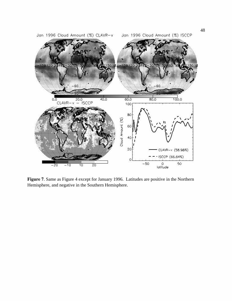
Figure 7. Same as Figure 4 except for January 1996. Latitudes are positive in the NorthernHemisphere, and negative in the Southern Hemisphere.

48

Figure 8. January 1996 zonal mean cloud amount from CLAVR-x (average of NOAA-14 and



49

Figure 9. Same as Figure 4 except fields shown for the cloud amount differences between July

1995 and January 1996. Latitudes are positive in the Northern Hemisphere, and negative in the

Southern Hemisphere.

50

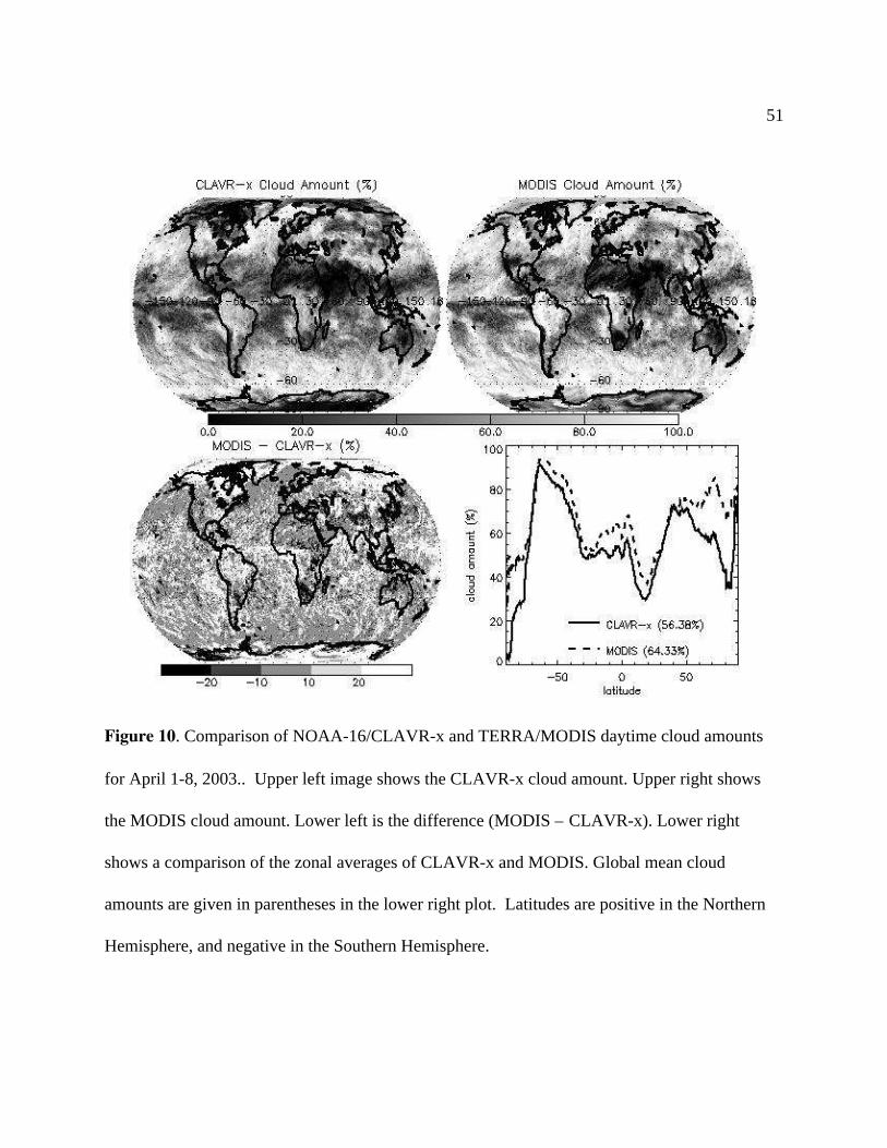
Figure 10. Comparison of NOAA-16/CLAVR-x and TERRA/MODIS daytime cloud amounts

for April 1-8, 2003.. Upper left image shows the CLAVR-x cloud amount. Upper right shows

the MODIS cloud amount. Lower left is the difference (MODIS – CLAVR-x). Lower right

shows a comparison of the zonal averages of CLAVR-x and MODIS. Global mean cloud

amounts are given in parentheses in the lower right plot. Latitudes are positive in the Northern


51

List of Tables

Table 1. Summary of the cloud masks used for each type of comparison, and the time periods

encompassed.

Table 2. Approximate daytime equator crossing times.

Table 3. July 1995 CLAVR-1 vs. CLAVR-x comparative statistics, for the average over the

ascending and descending orbits of NOAA-14.

Table 4. Total global cloud amount for July 1995 and Jan. 1996.

Table 5. Percentage of cloud mask for each cloud classification. Mean and standard deviation

are calculated over 7 random ascending orbits of NOAA-14, in July 1995.

Table 6. July 1995 ISCCP vs. CLAVR-x comparative statistics. CLAVR-x cloud mask data are

averaged over the ascending and descending orbits of either NOAA-12 or NOAA-14.

Table 7. January 1996 CLAVR-1 vs. CLAVR-x comparative statistics, for the average over the


52

Table 8. January 1996 ISCCP vs. CLAVR-x comparative statistics. CLAVR-x cloud mask data

are averaged over the ascending and descending orbits of either NOAA-12 or NOAA-14.

Table 9. Average of April 1-8, 2003 Terra MODIS vs. CLAVR-x comparative statistics, for the

average over the ascending and descending orbits of NOAA-14.

53

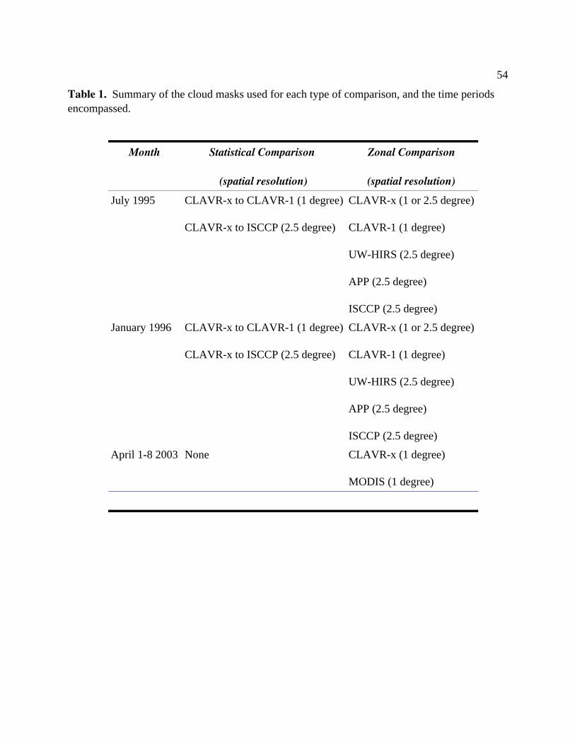
Table 1. Summary of the cloud masks used for each type of comparison, and the time periodsencompassed.

Month Statistical Comparison

(spatial resolution)

Zonal Comparison

(spatial resolution)

July 1995 CLAVR-x to CLAVR-1 (1 degree)

CLAVR-x to ISCCP (2.5 degree)

CLAVR-x (1 or 2.5 degree)

CLAVR-1 (1 degree)

UW-HIRS (2.5 degree)

APP (2.5 degree)

ISCCP (2.5 degree)

January 1996 CLAVR-x to CLAVR-1 (1 degree)

CLAVR-x to ISCCP (2.5 degree)

CLAVR-x (1 or 2.5 degree)

CLAVR-1 (1 degree)

UW-HIRS (2.5 degree)

APP (2.5 degree)

ISCCP (2.5 degree)

April 1-8 2003 None CLAVR-x (1 degree)

MODIS (1 degree)

54

Table 2. Approximate daytime equator crossing times

Daytime Equator Crossing

Time

NOAA-12 07:30 am

NOAA-14 04:30 pm

NOAA-16 01:30 pm

EOS-Terra 10:30 am

55

Table 3. July 1995 CLAVR-1 vs. CLAVR-x comparative statistics, for the average over the


NOAA-14 Global NOAA-14 60N-60SNOAA-14 poleward of

60N and 60S

S20 0.694 0.871 0.341

S-60 0.083 0.000 0.248

Sh 0.569 0.795 0.225

Srms 0.274 0.104 0.509

Sbias 0.080 -0.030 0.333

Sabs 0.170 0.079 0.384

56

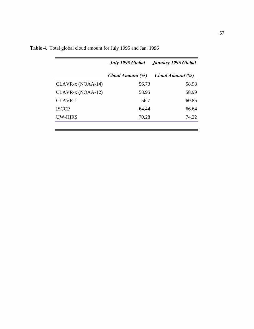
Table 4. Total global cloud amount for July 1995 and Jan. 1996

July 1995 Global

Cloud Amount (%)

January 1996 Global

Cloud Amount (%)

CLAVR-x (NOAA-14) 56.73 58.98

CLAVR-x (NOAA-12) 58.95 58.99

CLAVR-1 56.7 60.86

ISCCP 64.44 66.64

UW-HIRS 70.28 74.22

57

Table 5. Percentage of cloud mask for each cloud classification. Mean and standard deviation

are calculated over 7 random ascending orbits of NOAA-14, in July 1995.

Clear Mixed-

Clear

Mixed-

Cloudy

Cloudy

Mean (all clouds) 22.35 20.01 29.52 28.11

Standard Deviation

(all clouds) 2.64 1.47 2.53 1.64

Mean (water

clouds only) 13.07 23.48 31.14 32.43

Standard Deviation

(water clouds only) 1.29 2.09 2.43 2.12

58

Table 6. July 1995 ISCCP vs. CLAVR-x comparative statistics. CLAVR-x cloud mask data are

averaged over the ascending and descending orbits of either NOAA-12 or NOAA-14.

NOAA-14 GlobalNOAA-14 60N-

60S

NOAA-12

Global

NOAA-12 60N-

60S

S20 0.721 0.821 0.744 0.865

S-60 0.000 0.000 0.001 0.000

Sh 0.551 0.722 0.574 0.778

Srms 0.150 0.118 0.152 0.111

Sbias 0.068 0.080 0.048 0.060

Sabs 0.114 0.091 0.110 0.834

59

Table 7. January 1996 CLAVR-1 vs. CLAVR-x comparative statistics, for the average over the


NOAA-14 Global NOAA-14 60N-60SNOAA-14 poleward of

60N and 60S

S20 0.633 0.823 0.255

S-60 0.034 0.006 0.090

Sh 0.477 0.713 0.170

Srms 0.240 0.142 0.628

Sbias 0.095 -0.005 0.492

Sabs 0.170 0.099 0.506

60

Table 8. January 1996 ISCCP vs. CLAVR-x comparative statistics. CLAVR-x cloud mask data

are averaged over the ascending and descending orbits of either NOAA-12 or NOAA-14.

NOAA-14 GlobalNOAA-14 60N-

60S

NOAA-12

Global

NOAA-12 60N-

60S

S20 0.738 0.819 0.738 0.827

S-60 0.009 0.000 0.008 0.000

Sh 0.583 0.720 0.589 0.728

Srms 0.162 0.122 0.165 0.120

Sbias 0.047 0.083 0.058 0.081

Sabs 0.116 0.094 0.119 0.093

61

Table 9. Average of April 1-8, 2003 Terra MODIS vs. CLAVR-x comparative statistics, for the

average over the ascending and descending orbits of NOAA-14.

NOAA-14 Global NOAA-14 60N-60S

S20 0.647 0.777

S-60 0.013 0.000

Sh 0.519 0.645

Srms 0.204 0.129

Sbias 0.088 0.067

Sabs 0.143 0.094

62

Comparison of NOAA’s Operational AVHRR Derived Cloud...

Documents

Transcript of Comparison of NOAA’s Operational AVHRR Derived Cloud...