Comparison of Hydrates Formation Modeling Software

Performance

By

Ismail Ismail

Submitted for the degree of Master of Science in

Petroleum Engineering

Technical University of Crete

Crete, Greece

Heriot-Watt University

Edinburgh, Scotland

March, 2020

The copyright in this thesis is owned by the author. Any quotation from the thesis or use of any of

the information contained in it must acknowledge this thesis as the source of the quotation or in-

formation.

2

Abstract

Predicting hydrate stability/formation conditions is crucial for the oil and gas industry mainly

to avoid pipelines blockage during oil and gas transportation and supplying. Additionally, ex-

ploitation methods of the natural gas and CO2 storage in hydrates have started gaining attention

recently. Thus, understanding under what conditions hydrates are stable or can be stabilized is

very important. Based on that, accurate knowledge of hydrate modeling in the presence of salts,

inhibitors and non-ideal components is a main key in all related sectors.

In the first part of this work, various approaches/models available in the literature and in the

industry to describe hydrates thermodynamic behavior are presented and studied in detail so

that the differences in stability, solid solution theory of Van der Waals and Platteeuw and the

specific thermodynamic models representing all phases that co-exist (ice, water, solid CO2)

adopted in each approach are well understood.

Subsequently, the accuracy of the approaches describing the phase equilibria of gas hydrates

in the presence of CO2 components, high/low concentration of aqueous salt(s) and/or high/low

concentration of inhibitor(s) is evaluated. The approaches studied and tested are implemented

in four well known commercial software packages extensively used in the industry, that hold

the following industrial/developing name and the corresponding (approach): HydraFlash/Hy-

draFact (HF, HF72), MultiFlash/KBC (MF(CPA)/MF(RKSA), CSMGem (CSMGem),

CSMHyd (CSMHyd).

The accuracy comparison is run against a large database of experimentally measured hydrate

dissociation conditions which has been collected from papers that appeared in the literature

between 2015-2019. The collected experimental data has been reproduced using all six ap-

proaches and the obtained results have been utilized to evaluate the accuracy of each method

as a function of the temperature and pressure of the system.

The results obtained are analyzed in detail and the reasons explaining the accuracy/deviations

of each approach are presented. It has been found that the accuracy of the six studied ap-

proaches are ordered as follows (from most to less accurate): HF > HF72 > MF CPA > MF

RKSA> CSMGem > CSMHyd.

This copy is a Preliminary Version

3

Dedication

Dedicated to my Father Ali (1965-2003).

4

Acknowledgments

This thesis is submitted in partial fulfilment of the requirements for the MSc. degree at Technical

University of Crete. This work has been conducted with collaboration of Heriot Watt University,

HydraFact Company and National Technical University of Athens, under the supervision of Pro-

fessor Bahman Tohidi and Professor Vassilis Gaganis. The project has no fund or grants by any of

the institution or supervisor mentioned. However, a six-month free license for HydraFLASH Soft-

ware was provided by HydraFact Company, MultiFlash license from technical university of Crete

and both CSM software by Dr. Dimitris Marinakis.

I would like to thank my advisor, Professor Bahman Tohidi for providing me the opportunity to

work with such a scientifically interesting and challenging project. I would like also to thank Dr.

Ramin Mousavi for his help and guidance throughout this project but special and countless thanks

go to Professor Vassilis Gaganis for all his continuous help and support, his inspiring discussions,

and his huge enthusiasm during the time we worked together. Also, in this regard, I would like to

thank Professor Nikos Pasadakis for providing all necessary help during the course and his kind-

ness that allow me to continue my Master and be able to deliver this project. Additionally, I greatly

appreciate the help and leads of Dr.Dimitris Marinakis. As well as my friends from the Master

making my stay in Crete/Athens very pleasant and provided me with any help needed. At the end

but not at the least, I am grateful to my family members. Words cannot express anything on behalf

of them.

Ismail Ismail

5

A thesis submitted to the committee members

Date_________________

Signed: ______________________________

Approved: ______________________________

Date_________________

Signed: ______________________________

Approved: ______________________________

Date_________________

Signed: ______________________________

Approved: ______________________________

_____________________________

Dr. ……………………………………

6

Contents

Abstract ........................................................................................................................................................ 2

Dedication .................................................................................................................................................... 3

Acknowledgments ....................................................................................................................................... 4

Lists of Tables .............................................................................................................................................. 9

List of Figures ............................................................................................................................................ 10

Chapter 1 ................................................................................................................................................... 11

1 Introduction ............................................................................................................................................ 11

1.1 Gas Hydrate Technological Applications ..................................................................................... 12

1.2 Energy Storage in Gas Hydrates ................................................................................................... 12

1.3 Energy Recovery and Production of Natural Hydrates .............................................................. 12

1.4 Gas and Oil Production and Transportation (Flow Assurance) ................................................. 13

1.5 Gas Hydrate Structure and Composition ..................................................................................... 15

1.5.1 Clathrate Hydrates .................................................................................................................. 15

1.6 Main Points Describing the Importance of This Work for Oil and Gas Industry .................... 17

Chapter 2 ................................................................................................................................................... 18

2 Gibbs Energy Minimization and Stability Analysis ............................................................................ 18

2.1 Essence of The Problem .................................................................................................................. 18

2.2 Three-Step Application Procedure ................................................................................................ 19

Step 1: Translation of the Real Problem into an Abstract, Mathematical Problem ................... 19

Step 2: A Solution Is Found to the Mathematical Problem .......................................................... 20

Step 3: Translating Back the Mathematical Solution to A Real Physical Meaning .................... 20

2.3 Phase Equilibrium Criteria ............................................................................................................ 21

2.4 Phase Equilibria .............................................................................................................................. 21

2.4.1 Vapor-Liquid Equilibria ............................................................................................................. 21

2.4.1.1 Phase Boundary Determination Problem ........................................................................... 22

2.4.1.2 Relative Phase Quantity Determination .............................................................................. 22

2.4.1.3 Phase Quality Determination ............................................................................................... 22

2.4.1.4 Criteria for Chemical Equilibria in Terms of Fugacity..................................................... 23

2.4.1.5 Fugacity Coefficient .............................................................................................................. 24

2.4.1.6 Equilibrium and Equilibrium Ratios (Ki) .......................................................................... 25

2.4.1.7 Mass Balance ......................................................................................................................... 25

2.4.1.8 Analysis of the Objective Functions and the Need for Rachford-Rice Equation ............ 28

2.4.1.9 Obtaining Ki’s Equilibrium Ratios ...................................................................................... 30

2.4.1.10 Summary .............................................................................................................................. 30

2.4.1.11 Algorithm ............................................................................................................................. 32

7

2.5 Multiphase Equilibria ..................................................................................................................... 33

2.5.1 Thermodynamic Equilibrium Constraint and Equilibrium Ratios ........................................ 33

2.5.2 Gupta’s Approach ........................................................................................................................ 34

2.5.3 Mass Balance (Rachford-Rice Extension and Gupta’s Parameter Implementation) ............ 35

2.5.4 Solving For Thermodynamic Equilibrium ................................................................................ 36

2.5.4.1 Minimizing Gibbs Energy (At A Given Phase Fractions/Compositions) ......................... 37

2.5.4.2 Updating K-Values and Composition at A Given Gibbs Energy ...................................... 38

2.5.5 Ki’s Values for Hydrate Problem ............................................................................................... 38

2.5.6 Definition of the Reference Phase ............................................................................................... 39

2.5.7 Algorithm ...................................................................................................................................... 40

Chapter 3 ................................................................................................................................................... 41

3 Cubic Plus Association Eos ................................................................................................................... 41

3.1 Introduction ..................................................................................................................................... 41

3.2 Association Energy and Volume Parameters ............................................................................... 43

3.3 Association Term in CPA Eos ........................................................................................................ 44

3.3.1 Fraction of Non-Bonded Associating Molecules, XA ............................................................ 45

3.3.2 Association Schemes ................................................................................................................ 46

Chapter 4 ................................................................................................................................................... 50

4 Hydrates Thermodynamic Modelling .................................................................................................. 50

4.1 Introduction and Review of First Hydrate Prediction Methods ................................................. 50

4.2 Original Van Der Waals-Platteeuw Hydrate Model .................................................................... 51

4.2.1 Langmuir Adsorption Coefficient 𝑪𝑻𝒎, 𝒋 .............................................................................. 55

4.3 Parrish and Prausnitz Hydrate Modelling ................................................................................... 56

4.3.1 Model Theory ........................................................................................................................... 56

4.3.2 Algorithm for Hydrate Dissociation Pressure ....................................................................... 63

4.3.3 Improvement in Hydrate Modeling After Proposed Method of (Prausnitz W. 1972) ....... 63

4.4 Hydrate Model of Ballard 2002 ..................................................................................................... 64

4.4.1 Model Theory ............................................................................................................................... 64

4.4.1.1 Activity coefficient for water in hydrate ............................................................................. 65

4.4.1.2 Fugacity development ........................................................................................................... 66

4.4.1.3 Langmuir Constant ............................................................................................................... 67

4.5 MultiFlash and HydraFLASH® Hydrate Modelling .................................................................... 68

4.5.1 Model Theory ........................................................................................................................... 68

Chapter 5 ................................................................................................................................................... 71

5 Thermodynamic Models ........................................................................................................................ 71

5.1 Vapor Phase ..................................................................................................................................... 72

8

5.2 Liquid Hydrocarbon Phase ............................................................................................................ 78

5.3 Ice Phase .......................................................................................................................................... 82

5.3.2 Poynting Correction Method .................................................................................................. 83

5.3.3 Solid Freezeout-Model ............................................................................................................. 84

5.4 Aqueous Phase ................................................................................................................................. 85

5.4.1 Fugacity Models for Dissolved Gas ............................................................................................ 85

5.4.1.1 Classical Thermodynamic Treatment ................................................................................. 85

5.4.1.2 Eos Model .............................................................................................................................. 85

5.4.2 Fugacity Models for Water ......................................................................................................... 86

5.4.2.1 Classical Thermodynamic Treatment ................................................................................. 86

5.4.2.2 Eos Model .............................................................................................................................. 86

Chapter 6 ................................................................................................................................................... 88

6.1 Approaches Application ..................................................................................................................... 88

6.2 Background of the Study .................................................................................................................... 88

6.2.1 The Need of an Accurate Model for Co2 Hydrate ..................................................................... 89

6.3 Theory and Approaches ..................................................................................................................... 89

6.3.1 Approach Nº1: Parrish and Prausnitz (1972) “CSMHyd” ...................................................... 89

6.3.2 Approach Nº2: Ballard and Sloan (2002) “CSMGem” ............................................................ 90

6.3.3 Approach Nº3: KBC/MultiFlash RKSA “MF RKSA” ............................................................. 91

6.3.4 Approach N#4: KBC/MultiFlash CPA “MF CPA” .................................................................. 92

6.3.5 Approach Nº5&6: HydraFLASH/HydraFact CPA, Both Approaches “HF” & “HF72” ..... 93

6.4 Experimental Work ............................................................................................................................ 93

6.4.1 Methodology ................................................................................................................................. 93

6.4.2 Error Indices ................................................................................................................................ 94

6.5 Results and Discussion ........................................................................................................................ 94

6.5.1 Effect of Temperature (HF, HF72, MF(CPA) And MF (RKSA)) ........................................... 95

6.5.1.1 A1 Series (Low Temperature [273-283 K]) ......................................................................... 95

6.5.1.2 A2 Series (High Temperature [283-295 K]) ........................................................................ 97

6.5.2 Effect of Temperature (HF, HF72, MF(CPA), MF (RKSA) ,Csmgem And Csmhyd) ........ 100

6.5.2.1 B1 Series (Low Temperature [273-283 K]) ....................................................................... 100

6.5.2.1 B2 Series (High Temperature [283-293.95 K]) ................................................................. 102

6.7 Conclusion ..................................................................................................................................... 103

References ............................................................................................................................................ 105

9

Lists of Tables

Table 1 Constants reported by (Prausnitz W. 1972) for reference hydrate dissociation pressure calculation………..59

Table 2 Kihara Parameters reported by (Prausnitz W. 1972) used in CSMHyd ......................................................... 60

Table 3 Parameters for calculating Langmuir constant for structure sI & sII (Prausnitz W. 1972) ............................ 62

Table 4 Formation properties of empty hydrate .......................................................................................................... 66

Table 5 Kihara Parameters reported by (Sloan ED 2008) used in CSMGem ............................................................. 68

Table 6 Kihara Parameters reported by (Tohidi-Kalorazi 1995) used in HydraFLAS ................................................ 69

Table 7 Kihara Parameters reported by (H.Haghighi 2009) for ice co-existence phase used in HydraFLASH .......... 69

Table 8 Fugacity coefficient for three cubic EoS ........................................................................................................ 77

10

List of Figures

Figure 1 Schematic of the pressure and temperature conditions of fluids (gas/water/oil) in a subsea pipeline and the

gas hydrate formation/stability region ......................................................................................................................... 13

Figure 2 Cavities which combine to form different hydrate structures A)512 B)435663 C)51268 D) 51262 E)51264 ...... 16

Figure 3 Combination of cages to form each hydrate structure ................................................................................... 16

Figure 4 Problem Statement. ...................................................................................................................................... 18

Figure 5 Three-step application of thermodynamics to phase-equilibrium problems. ................................................ 19

Figure 6 Two phase system ........................................................................................................................................ 27

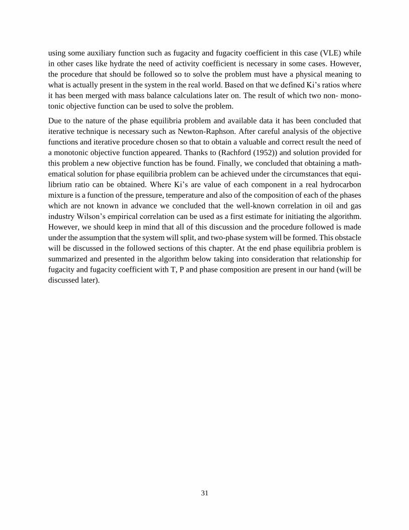
Figure 7 Typical Algorithm for Two phase flash system (produced in this work). .................................................... 32

Figure 7 Illustrative phase diagram for gas hydrates. Lines correspond to three-phase equilibrium, separating the two-

phase regions. The label corresponds to liquid water (Lw), ice (I), hydrate (H), vapor (V) and liquid hydrocarbons

(LHC).The intersection of the three-phase lines corresponds to the quadruple point (Q1) and (Q2), where I-Lw-H-V

and Lw-H-V-LHC coexist respectively (Sloan ED 2008) ........................................................................................... 39

Figure 8 Algorithm for multiphase flash problems including Gupta’s stability analysis (produced in this work). .... 40

Figure 9 Model of hard spheres with a single associating site A illustrating a simple case of molecular association due

to short-distance, highly orientational, site-site attraction (Chapman W.G. (1990)). ................................................. 43

Figure 10 Models of hard sphere (monomer) and chain (m-mer.) molecules with two associating sites A and B; the

chain molecule represents non- spherical molecule (Chapman W.G. (1990)). ............................................................ 44

Figure 11 Types of bonding in real associating fluids (Huang S.H. (1990)) .............................................................. 47

Figure 12 association sites for alkanol and water ....................................................................................................... 48

Figure 13 Illustration of Equation (4. 5) stating vdW-P concerning difference of metastable and actual hydrate phase

(picture belong to this work)........................................................................................................................................ 53

Figure 15 Original vdW-P not accounting for no distortion of lattice structure (produced) ....................................... 65

Figure 16 (A.L Ballard 2002) Modified model accounting for distortion of lattice structure (produced) .................. 66

Figure 18 P-v diagram of a pure component............................................................................................................... 79

Figure 19 V Poynting correction factor for water (pressure and temperature effect) (M. D. Koretsky n.d.) .............. 80

Figure 20 Cumulative Average Absolute Relative Error (%) vs. temperature (K) [273.0-283 K] ............................. 95

Figure 21 Cumulative Absolute Relative Error (%) vs temperature (K) [273.0-283 K] ............................................. 95

Figure 22 Cumulative Average Absolute Error (MPa) vs. temperature (K) [273.0-283 K] ....................................... 96

Figure 23 Cumulative Absolute Error (MPa) vs temperature (K) [273-283 K] .......................................................... 96

Figure 24 Cumulative Average Absolute Relative Error (%) vs. temperature (K) [283-293.95 K] ........................... 97

Figure 25 Cumulative Absolute Relative Error (%) vs temperature (K) [283.0-293.95 K] ........................................ 98

Figure 26 Cumulative Average Absolute Error (MPa) vs. temperature (K) [283.0-293.95 K] .................................. 98

Figure 27 Cumulative Absolute Error (MPa) vs temperature (K) [283-293.95 K] ..................................................... 99

Figure 28 Cumulative Absolute Relative Error (%) vs temperature (K) [273.0-283 K] ........................................... 100

Figure 29 Cumulative Absolute Error (MPa) vs temperature (K) [273-283 K] ........................................................ 101

Figure 30 Cumulative Absolute Relative Error (%) vs temperature (K) [283.0-293.95 K] ...................................... 102

Figure 29 Cumulative Absolute Error (MPa) vs temperature (K) [283-293.95 K] ................................................... 102

11

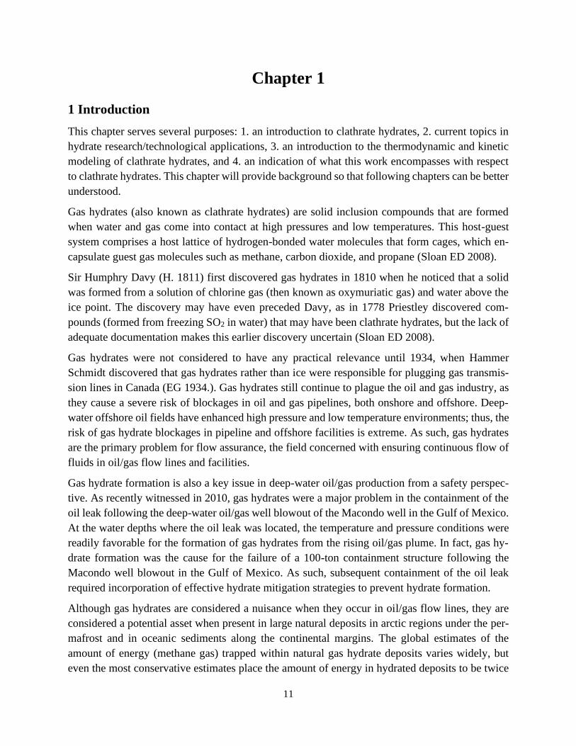
Chapter 1

1 Introduction

This chapter serves several purposes: 1. an introduction to clathrate hydrates, 2. current topics in

hydrate research/technological applications, 3. an introduction to the thermodynamic and kinetic

modeling of clathrate hydrates, and 4. an indication of what this work encompasses with respect

to clathrate hydrates. This chapter will provide background so that following chapters can be better

understood.

Gas hydrates (also known as clathrate hydrates) are solid inclusion compounds that are formed

when water and gas come into contact at high pressures and low temperatures. This host-guest

system comprises a host lattice of hydrogen-bonded water molecules that form cages, which en-

capsulate guest gas molecules such as methane, carbon dioxide, and propane (Sloan ED 2008).

Sir Humphry Davy (H. 1811) first discovered gas hydrates in 1810 when he noticed that a solid

was formed from a solution of chlorine gas (then known as oxymuriatic gas) and water above the

ice point. The discovery may have even preceded Davy, as in 1778 Priestley discovered com-

pounds (formed from freezing SO2 in water) that may have been clathrate hydrates, but the lack of

adequate documentation makes this earlier discovery uncertain (Sloan ED 2008).

Gas hydrates were not considered to have any practical relevance until 1934, when Hammer

Schmidt discovered that gas hydrates rather than ice were responsible for plugging gas transmis-

sion lines in Canada (EG 1934.). Gas hydrates still continue to plague the oil and gas industry, as

they cause a severe risk of blockages in oil and gas pipelines, both onshore and offshore. Deep-

water offshore oil fields have enhanced high pressure and low temperature environments; thus, the

risk of gas hydrate blockages in pipeline and offshore facilities is extreme. As such, gas hydrates

are the primary problem for flow assurance, the field concerned with ensuring continuous flow of

fluids in oil/gas flow lines and facilities.

Gas hydrate formation is also a key issue in deep-water oil/gas production from a safety perspec-

tive. As recently witnessed in 2010, gas hydrates were a major problem in the containment of the

oil leak following the deep-water oil/gas well blowout of the Macondo well in the Gulf of Mexico.

At the water depths where the oil leak was located, the temperature and pressure conditions were

readily favorable for the formation of gas hydrates from the rising oil/gas plume. In fact, gas hy-

drate formation was the cause for the failure of a 100-ton containment structure following the

Macondo well blowout in the Gulf of Mexico. As such, subsequent containment of the oil leak

required incorporation of effective hydrate mitigation strategies to prevent hydrate formation.

Although gas hydrates are considered a nuisance when they occur in oil/gas flow lines, they are

considered a potential asset when present in large natural deposits in arctic regions under the per-

mafrost and in oceanic sediments along the continental margins. The global estimates of the

amount of energy (methane gas) trapped within natural gas hydrate deposits varies widely, but

even the most conservative estimates place the amount of energy in hydrated deposits to be twice

12

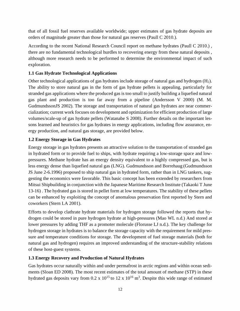
that of all fossil fuel reserves available worldwide; upper estimates of gas hydrate deposits are

orders of magnitude greater than those for natural gas reserves (Paull C 2010.).

According to the recent National Research Council report on methane hydrates (Paull C 2010.) ,

there are no fundamental technological hurdles to recovering energy from these natural deposits ,

although more research needs to be performed to determine the environmental impact of such

exploration.

1.1 Gas Hydrate Technological Applications

Other technological applications of gas hydrates include storage of natural gas and hydrogen (H2).

The ability to store natural gas in the form of gas hydrate pellets is appealing, particularly for

stranded gas applications where the produced gas is too small to justify building a liquefied natural

gas plant and production is too far away from a pipeline (Andersson V 2000) (M. M.

GudmundssonJS 2002). The storage and transportation of natural gas hydrates are near commer-

cialization; current work focuses on development and optimization for efficient production of large

volumes/scale-up of gas hydrate pellets (Watanabe S 2008). Further details on the important les-

sons learned and heuristics for gas hydrates in energy applications, including flow assurance, en-

ergy production, and natural gas storage, are provided below.

1.2 Energy Storage in Gas Hydrates

Energy storage in gas hydrates presents an attractive solution to the transportation of stranded gas

in hydrated form or to provide fuel to ships, with hydrate requiring a low-storage space and low-

pressures. Methane hydrate has an energy density equivalent to a highly compressed gas, but is

less energy dense than liquefied natural gas (LNG). Gudmundsson and Borrehaug (Gudmundsson

JS June 2-6.1996) proposed to ship natural gas in hydrated form, rather than in LNG tankers, sug-

gesting the economics were favorable. This basic concept has been extended by researchers from

Mitsui Shipbuilding in conjunction with the Japanese Maritime Research Institute (Takaoki T June

13-16) . The hydrated gas is stored in pellet form at low temperatures. The stability of these pellets

can be enhanced by exploiting the concept of anomalous preservation first reported by Stern and

coworkers (Stern LA 2001).

Efforts to develop clathrate hydrate materials for hydrogen storage followed the reports that hy-

drogen could be stored in pure hydrogen hydrate at high-pressures (Mao WL n.d.) And stored at

lower pressures by adding THF as a promoter molecule (Florusse LJ n.d.). The key challenge for

hydrogen storage in hydrates is to balance the storage capacity with the requirement for mild pres-

sure and temperature conditions for storage. The development of fuel storage materials (both for

natural gas and hydrogen) requires an improved understanding of the structure-stability relations

of these host-guest systems.

1.3 Energy Recovery and Production of Natural Hydrates

Gas hydrates occur naturally within and under permafrost in arctic regions and within ocean sedi-

ments (Sloan ED 2008). The most recent estimates of the total amount of methane (STP) in these

hydrated gas deposits vary from 0.2 x 1015 to 12 x 1016 m3. Despite this wide range of estimated

13

gas, all estimates are significant when compared to evaluations of the conventional gas reserve of

0.15 x 1015 m3 methane (STP) (M. 2000). In the United States the mean hydrate value indicates

300 times more hydrated gas than the gas in the total remaining recoverable conventional reserves.

Hydrate reservoirs are considered a substantial future energy resource due to the large amount of

hydrated gas in these deposits, coupled with hydrates concentrating methane (at STP) by as much

as a factor of 164 and requiring less than 15% of the recovered energy for dissociation. However,

energy recovery is an engineering challenge.

Three general heuristics (Trehu AM 2006) for naturally occurring ocean hydrates are:

1. Water depths of 300-800 m (depending on the local bottom water temperature) are sufficient

to stabilize the upper hydrate boundary.

2. Biogenic hydrates predominate, with only a few sites comprising thermogenic hydrates (con-

taining CH4 and higher hydrocarbons), such as in the Gulf of Mexico, Cascadia and in the

Caspian Sea. These thermo genic deposits tend to comprise large accumulations near the sea

floor.

3. Hydrates are typically found where organic carbon accumulates rapidly, mainly in continental

shelves and enclosed seas. These are biogenic hydrates (containing CH4, formed from bacterial

methanogenesis). More details of the mechanism of generation of Bio & thermogenic gas in

(Sloan ED 2008)

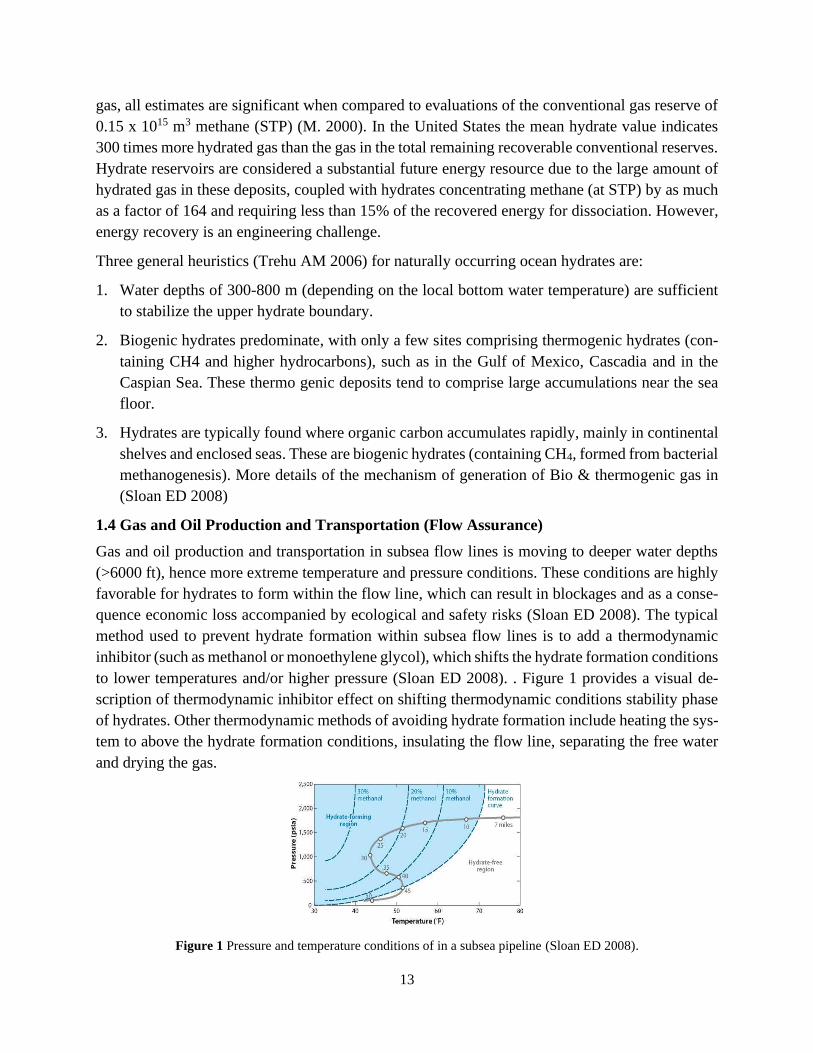
1.4 Gas and Oil Production and Transportation (Flow Assurance)

Gas and oil production and transportation in subsea flow lines is moving to deeper water depths

(>6000 ft), hence more extreme temperature and pressure conditions. These conditions are highly

favorable for hydrates to form within the flow line, which can result in blockages and as a conse-

quence economic loss accompanied by ecological and safety risks (Sloan ED 2008). The typical

method used to prevent hydrate formation within subsea flow lines is to add a thermodynamic

inhibitor (such as methanol or monoethylene glycol), which shifts the hydrate formation conditions

to lower temperatures and/or higher pressure (Sloan ED 2008). . Figure 1 provides a visual de-

scription of thermodynamic inhibitor effect on shifting thermodynamic conditions stability phase

of hydrates. Other thermodynamic methods of avoiding hydrate formation include heating the sys-

tem to above the hydrate formation conditions, insulating the flow line, separating the free water

and drying the gas.

Figure 1 Pressure and temperature conditions of in a subsea pipeline (Sloan ED 2008).

14

However, in many deep-water production scenarios, thermodynamic inhibition can become une-

conomical and even prohibitive due to the high concentrations of inhibitor required. Therefore,

flow assurance is progressively moving away from avoidance (thermodynamic control) of hydrate

formation toward risk management (kinetic control) which may allow hydrates to form, while pre-

venting a hydrate blockage (Sloan ED 2008).

Hydrate plugs are not typically formed during normal flow line operation by design. However,

plugs can occur due to the following abnormal flow line operations:

1. When the water phase is uninhibited as a result of inhibitor injection failure, dehydrator failure,

or the production of excess water,

2. During startup following an emergency shut-in performed due to system failure or adverse

weather conditions, such as a hurricane, or

3. When water-wet gas expands rapidly through a valve, orifice or other restriction, resulting in

significant Joule- Thomson cooling at under-inhibited conditions.

New technologies currently (Sloan ED 2008) being developed to control hydrate formation within

deep-water flowlines during normal and abnormal operations include:

1. The addition of low dosage hydrate inhibitors (LDHIs) that are effective at concentrations be-

low about 1 wt. %.12 there are two broad classes of LDHIs: kinetic hydrate inhibitors (KHIs)

and antiagglomerants (AAs). KHIs (e.g. poly-N-vinyl-caprolactam) operate by delaying nu-

cleation and/or crystal growth. AAs (e.g., quaternary ammonium salts) prevent hydrate crystals

from agglomerating to form a blockage, by maintaining the hydrates in the form of a suspended

slurry which allows fluid flow to occur unimpeded.

2. ‘‘Cold flow’’, denotes the process, whereby hydrates could be pumped as a slurry through the

flow line without the need for chemical inhibitors. Sintef-BP researchers have reported that the

addition of water to a flow of dry hydrate results in the formation of further dry hydrate. It is

suggested that capillary attractive forces between dry hydrates are low; hence, these particles

should not agglomerate to form a plug. This economic technique of risk-management appears

promising.

3. Hydrate plug remediation methods include depressurizing the line, injecting a thermodynamic

inhibitor, or electrical heating. Plug dissociation occurs radially and dissociation times can be

predicted using a Fourier’s Law model (e.g., CSMPlug). However, single-sided plug depres-

surization can be life-threatening due to the potential for a pressure- driven projectile and,

therefore, safety should be a major consideration. Unlike one-sided dissociation, careful two-

sided dissociation normally eliminates the concern of having a projectile in the pipeline.

The thermodynamics of hydrate formation is well-established, with a number of reliable and ade-

quately accurate prediction programs available (e.g., HydraFlash, MultiFlash, CSMHyd,

CSMGem) using different models. However, the time-dependent processes of hydrate formation

and decomposition are still poorly understood. A major challenge is predicting the time required

15

for hydrate crystals to nucleate, grow, agglomerate and eventually form a hydrate plug in a transi-

ent, multiphase flow line.

Hydrate nucleation studies are particularly challenging due to the stochastic, microscopic nature

of the nucleation process, which involves 10s to 1,000s of molecules. Nucleation and hydrate in-

duction (formation) times are affected by a number of variables, including: apparatus geometry,

surface area, water contaminants and history and the degree of agitation or turbulence. This makes

it very difficult to transfer the results from one laboratory or flow loop facility to another. The

question of transferability and scale-up to field conditions is even more daunting. Therefore, being

able to predict when hydrates will nucleate and grow is a major challenge which is critical to

assessing the risk of hydrate formation.

For hydrate formation in liquid hydrocarbon systems, fundamental understanding of the chemistry

of the system (water- in-oil and oil-in-water emulsion chemistry and interfacial interactions) cou-

pled with multiphase flow is needed. The phenomenon of hydrate particle agglomeration is key to

determining the risk of hydrate plug formation.

1.5 Gas Hydrate Structure and Composition

1.5.1 Clathrate Hydrates

Clathrate hydrates are non-stoichiometric crystalline compounds that consist of a hydrogen bonded

network of water molecules and enclathrated molecules. Davy (H. 1811) first observed clathrate

hydrates in the chlorine + water system. It wasn’t until 1934, however, that clathrate hydrates were

extensively studied. Hammerschmidt (EG 1934.) Found that natural gas transport lines could be

blocked by the formation of clathrate hydrates. This raised a lot of attention in the oil and gas

industry, prompting more research to be performed on clathrate hydrates of natural gas. With the

majority of research being done on clathrate hydrates of natural gas, clathrate hydrates are typically

referred to as natural gas hydrates.

Natural gas hydrates are formed when natural gas is brought into contact with water, generally at

low temperatures and high pressures. The guest molecules most common in natural gas systems

are hydrocarbons ranging from methane to i-pentane. These gases make up greater than 98 mole

percent of a typical natural gas in United States pipelines. Therefore, the majority of the experi-

mental work performed in the last 70 years has been for hydrates of hydrocarbons ranging from

methane to i-pentane (Sloan ED 2008).

There are three basic hydrate structures known to form from natural gases: structure I (sI), structure

II (sII) and structure H (sH). The type of hydrate that forms depends on the size of the gas mole-

cules included in the hydrate. In general, small molecules such as methane or ethane form sI hy-

drates as single guests, larger molecules such as propane and i-butane form sII hydrates, and even

larger molecules such as i- pentane form sH hydrates in the presence of a small “help” molecule

such as methane. When sI, sII and sH hydrate formers are in a mixture, it is not easy to generalize

which hydrate structure will be present. However, the type of hydrate that forms will depend on

the composition, temperature and pressure of the system (Sloan ED 2008).

16

The basic "building block" of each of these structures is the pentagonal dodecahedron, which is a

12-sided pentagonal faced polyhedral (5). There are twenty water molecules in this cage with the

oxygen atoms at each vertex and the hydrogen atoms either chemically or hydrogen bonded be-

tween each oxygen atom. The bonds between the hydrogen and oxygen molecules essentially hold

the cage together and the guest molecules serve to keep it from collapsing. Depending on what

gases are present and ultimately which hydrate structure is formed; these basic cages stack to form

more complex cages. For sI hydrates they form tetra decahedron cages that have 12 pentagonal

and 2 hexagonal faces (5 6). For sII hydrates, hexadecachoron cages are formed; 12 pentagonal

and 4 hexagonal faces (5 6). For sH hydrates, two new cages are formed which are, using the

previous nomenclature for a cage, 435663 and 51268. Figure 2 provides a visual description of each

hydrate cage.

Figure 2 Cavities which combine to form different hydrate structures A)512 B)435663 C)51268 D) 51262 E)51264

A unit cell of a particular hydrate structure is specified by how the respective cages combine to

form a periodic crystalline lattice. Figure 3 shows how the various cages are arranged to form a

unit cell of each of the three most common structures.

For example, one-unit cell of sI hydrate contains 2 512 cages and 6 51262 cages. Notice that the

relative amount of small (512) cages varies within each hydrate structure. For instance, sI hydrates

are comprised of one-quarter 512 cages, sII hydrates are comprised of two-thirds and sH hydrates

are comprised of one-half. Differences between the hydrate structures such as this play a major

role in stability considerations.

Figure 3 Combination of cages to form each hydrate structure

17

1.6 Main Points Describing the Importance of This Work for Oil and Gas Industry

Natural gas looks set to become the world’s most important energy source within a decade. The

market size for oil and gas pipeline construction experienced tremendous growth prior to the eco-

nomic downturn in 2008. After faltering in 2009, demand for pipeline expansion and updating

increased the following year as energy production grew. Natural gas hydrates are responsible for

pipeline plugging and corrosion. Thus, handling the issue of the formation is a matter of vital

importance for the industry. Based on that and in order to provide the optimal strategy in dealing

with hydrate formation, it is of vital importance for the industry to have an understanding of the

conditions that cause hydrate formation. In the other hand, in all the gas hydrate technological

applications, it is clear that the paradigm is focusing on thermodynamics (time-independent prop-

erties) modeling and hydrate formation and dissociation properties. Improved understanding and

control of the thermodynamics of these processes are key factors to advancing the technologies

required in:

• Maintaining flow in pipelines by assessing the statics of hydrate formation, e.g. determining

when a hydrate plug will occur.

• Accurately predicting the type of gas hydrates forms: Hydrate I, II or H as well as the complex

phase transitions among the fluid and hydrate phases (e.g.: transition of hydrate structure II

to I).

• Reducing operational costs (OPEX) for the industry by accurately predicting hydrate for-

mation conditions as well as hydrate inhibition effect on hydrate formation condition such as:

Methanol, ethanol, MEG, DEG and TEG.

• Gas recovery from hydrate deposits by assessing the techniques needed to dissociate and re-

lease the gas from the deposit at specific thermodynamic conditions.

• Assessing submarine hydrate dissolution rates and the impact of this dissociation to the envi-

ronment.

In addition, the need of a reliable flow assurance engineering approach/tool will enable reservoir

engineers as well as process engineers to optimize detailed field planning activities such as:

• Quantifying the risks and problems arising from hydrate formation.

• Life field study on inhibitor requirement and formulation of hydrate presenting strategies.

18

Chapter 2

2 Gibbs Energy Minimization and Stability Analysis

A clear understanding of the thermodynamic properties of gas hydrate systems is critical in all gas

hydrate applications, from determining the temperature and pressure conditions at which a pipeline

will be within the hydrate stability zone, to assessing the conditions necessary to dissociate a gas

hydrate plug in a pipeline or a natural gas hydrate reservoir for energy production, to simply es-

tablishing the conditions at which a gas hydrate system can be synthesized in the laboratory. Gas

hydrate stability depends on temperature, pressure, gas composition and condensed phase compo-

sition (including liquid hydrocarbon phase, salt content and chemical inhibitor concentration).

Therefore, a method to calculate dissociation pressure and temperature and in particular hydrate

properties at any pressure and temperature is desired. This chapter discusses the approach taken to

perform these types of calculation using minimization of Gibbs energy of the system.

2.1 Essence of The Problem

We want to relate quantitatively the variables that describe the state of equilibrium of two or more

homogeneous phases (intensive properties are everywhere the same) that are free to interchange

energy and matter. We are concerned primarily with the intensive properties temperature, density,

pressure and composition (mole fractions). We want to describe the state of two or more phases

that are free to interact and that have reached a state of equilibrium. Then, given some of the

equilibrium properties of the two phases, our task is to predict those that remain.

Figure 4 Problem Statement.

Our problem might be characterized by other combinations of known and unknown variables. The

number of intensive properties that must be specified to fix unambiguously the state of equilibrium

is given by the Gibbs phase rule. In the absence of chemical reactions, the phase rule is:

Number of independent intensive properties = Number of components - Number of phases + 2

The questions that may raise here:

▪ How shall we go about solving the problem illustrated in Fig. 4?

19

▪ What theoretical framework is available to give us a basis for finding a solution?

When this question is raised, we turn to thermodynamics.

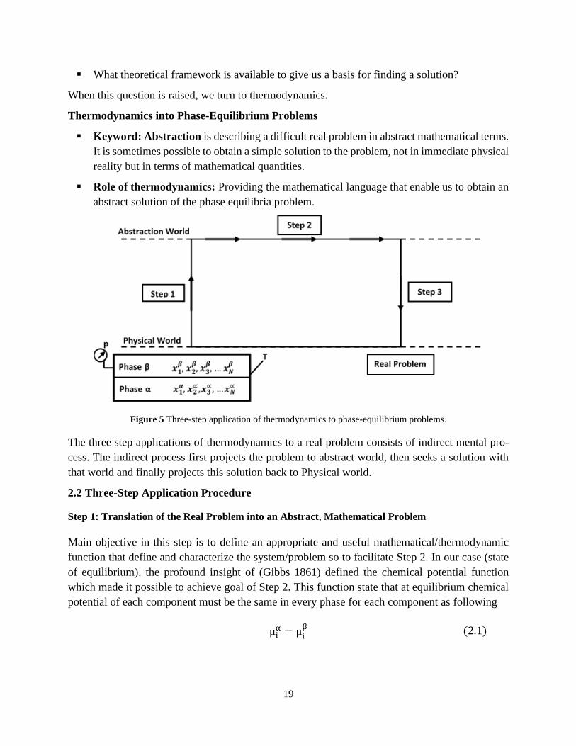
Thermodynamics into Phase-Equilibrium Problems

▪ Keyword: Abstraction is describing a difficult real problem in abstract mathematical terms.

It is sometimes possible to obtain a simple solution to the problem, not in immediate physical

reality but in terms of mathematical quantities.

▪ Role of thermodynamics: Providing the mathematical language that enable us to obtain an

abstract solution of the phase equilibria problem.

Figure 5 Three-step application of thermodynamics to phase-equilibrium problems.

The three step applications of thermodynamics to a real problem consists of indirect mental pro-

cess. The indirect process first projects the problem to abstract world, then seeks a solution with

that world and finally projects this solution back to Physical world.

2.2 Three-Step Application Procedure

Step 1: Translation of the Real Problem into an Abstract, Mathematical Problem

Main objective in this step is to define an appropriate and useful mathematical/thermodynamic

function that define and characterize the system/problem so to facilitate Step 2. In our case (state

of equilibrium), the profound insight of (Gibbs 1861) defined the chemical potential function

which made it possible to achieve goal of Step 2. This function state that at equilibrium chemical

potential of each component must be the same in every phase for each component as following

μiα = μi

β (2.1)

20

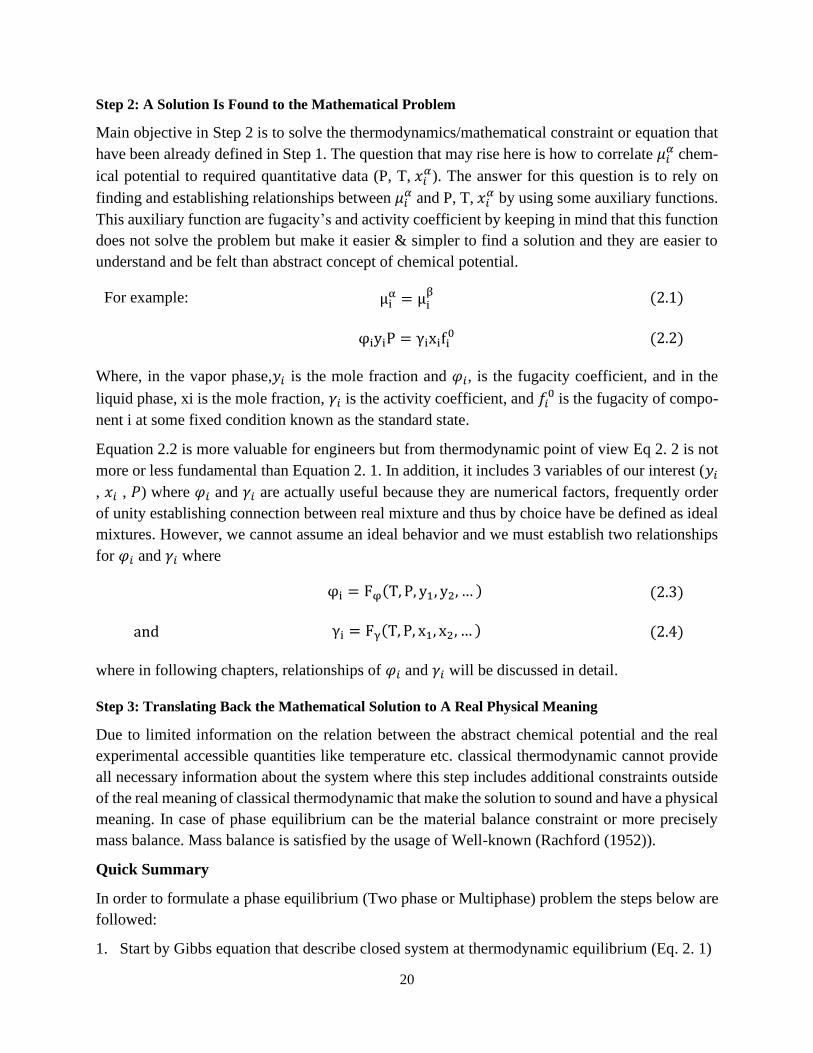
Step 2: A Solution Is Found to the Mathematical Problem

Main objective in Step 2 is to solve the thermodynamics/mathematical constraint or equation that

have been already defined in Step 1. The question that may rise here is how to correlate 𝜇𝑖𝛼 chem-

ical potential to required quantitative data (P, T, 𝑥𝑖𝛼). The answer for this question is to rely on

finding and establishing relationships between 𝜇𝑖𝛼 and P, T, 𝑥𝑖

𝛼 by using some auxiliary functions.

This auxiliary function are fugacity’s and activity coefficient by keeping in mind that this function

does not solve the problem but make it easier & simpler to find a solution and they are easier to

understand and be felt than abstract concept of chemical potential.

Where, in the vapor phase,𝑦𝑖 is the mole fraction and 𝜑𝑖, is the fugacity coefficient, and in the

liquid phase, xi is the mole fraction, 𝛾𝑖 is the activity coefficient, and 𝑓𝑖0 is the fugacity of compo-

nent i at some fixed condition known as the standard state.

Equation 2.2 is more valuable for engineers but from thermodynamic point of view Eq 2. 2 is not

more or less fundamental than Equation 2. 1. In addition, it includes 3 variables of our interest (𝑦𝑖

, 𝑥𝑖 , 𝑃) where 𝜑𝑖 and 𝛾𝑖 are actually useful because they are numerical factors, frequently order

of unity establishing connection between real mixture and thus by choice have be defined as ideal

mixtures. However, we cannot assume an ideal behavior and we must establish two relationships

for 𝜑𝑖 and 𝛾𝑖 where

where in following chapters, relationships of 𝜑𝑖 and 𝛾𝑖 will be discussed in detail.

Step 3: Translating Back the Mathematical Solution to A Real Physical Meaning

Due to limited information on the relation between the abstract chemical potential and the real

experimental accessible quantities like temperature etc. classical thermodynamic cannot provide

all necessary information about the system where this step includes additional constraints outside

of the real meaning of classical thermodynamic that make the solution to sound and have a physical

meaning. In case of phase equilibrium can be the material balance constraint or more precisely

mass balance. Mass balance is satisfied by the usage of Well-known (Rachford (1952)).

Quick Summary

In order to formulate a phase equilibrium (Two phase or Multiphase) problem the steps below are

followed:

1. Start by Gibbs equation that describe closed system at thermodynamic equilibrium (Eq. 2. 1)

For example: μiα = μi

β (2.1)

φiyiP = γixifi0 (2.2)

φi = Fφ(T, P, y1, y2, … ) (2.3)

and γi = Fγ(T, P, x1, x2, … ) (2.4)

21

2. Translate Gibbs equation of the real problem into an abstract mathematical problem using ther-

modynamics relationships and taking into consideration given information and required ones.

3. Correlate chemical potential 𝜇𝑖 to P, T using appropriate auxiliary equations for your case.

4. Add necessary constraints that make your problem physically valuable so to complete formu-

lation of your problem.

Result: Thermodynamic equilibrium is formulated mathematically. Problem solved

2.3 Phase Equilibrium Criteria

Based on what we have discussed in section before and in order to calculate thermodynamic equi-

librium for a closed system, two fundamental conditions must be met:

1. Equality of chemical potential of each component in each phase present.

2. Material balance is satisfied.

Where the first condition results from the Gibbs energy being at a minimum (Gibbs 1861). These

conditions are commonly used in developing procedures for solving for thermodynamic equilib-

rium. The most common implementation of these conditions is for the two-phase system, vapor

and liquid hydrocarbon, known as the VLE Flash. Where the requirement that the Gibbs energy of

the system must be at a minimum, at a given temperature and pressure, is a statement of the second

law of thermodynamics.

2.4 Phase Equilibria

In the following part we are going to look at phase equilibria problem from petroleum engineering

(reservoir engineering) point of view. After that we are going to extend the basis of VLE two phase

equilibria to Multiphase flash present implemented in hydrate modelling.

2.4.1 Vapor-Liquid Equilibria

As far as VLE is concerned, we can list a number of systems that are at the heart of petroleum fluid

production that involve this phenomenon such as Separators, Reservoir, Pipelines, Wellbore, LNG

Processing, NGL Processing, Storage, Oil and LNG Tankers.

Vapor/liquid equilibrium pertains to all aspects of petroleum production with which we are con-

cerned. It is no wonder, then, that we devote a new module to the subject itself.

In a typical problem of liquid and vapor coexistence, we are usually required to know one or more

of the following:

▪ The phase boundaries,

▪ The extent of each phase,

▪ The quality of each phase.

The main emphasis is on the quantitative prediction of the above. These three represent the three

basic types of VLE problems. A more detailed description of each of them is given below.

22

2.4.1.1 Phase Boundary Determination Problem

These types of problems are either a bubble-point or a dew-point calculation. They are mathemat-

ically stated as follows:

• Bubble-point T calculation: Given liquid composition (xi) and pressure (P), determine the

equilibrium temperature (T),

• Bubble-point P calculation: Given liquid composition (xi) and temperature (T), determine the

equilibrium pressure (P),

• Dew-point T calculation: Given vapor composition (yi) and pressure (P), determine the equi-

librium temperature (T),

• Dew-point P calculation: Given vapor composition (yi) and temperature (T), determine the

equilibrium pressure (P).

2.4.1.2 Relative Phase Quantity Determination

In this type of problem, overall composition (zi), pressure (P) and temperature (T) are given and

the extent of the phases (molar fractions of gas and liquid) are required.

2.4.1.3 Phase Quality Determination

In this type of problem, overall composition (zi), pressure (P), and temperature (T) are given and

the composition of the liquid and vapor phases is required.

Problems of types 5.1.2 and 5.1.3 are collectively referred to as flash calculation problems. All

three are problems that we encounter in production & reservoir operations as petroleum engineers.

Our focus now is on solving these sorts of problems. We want to use a predictive approach to do

so but One of the most difficult aspects of making VLE calculations is knowing whether a mixture

will actually split into two (or more) phases at the specified pressure and temperature. Tradition-

ally, this problem has been solved either by conducting a two-phase flash or by making a satura-

tion-pressure calculation. Both methods are expensive and not entirely reliable. In 1982, (M.

Michelsen (1982a)), (M. Michelsen (1982b)) showed how the Gibbs tangent-plane criterion could

be used to establish the thermodynamic stability of a phase (whether a given composition has a

lower energy remaining as a single phase (stable) or whether the mixture Gibbs energy will de-

crease by splitting the mixture into two or more phases (unstable)). (Baker (1982)) Shows graph-

ically how the Gibbs tangent-plane criterion is used to establish phase stability of simple binary

systems and (M. Michelsen (1982a))gives an algorithm to establish phase stability numerically.

This issue is going to be discussed later on. The algorithms presented in this section assume that a

mathematical solution to the two-phase problem exists: either a solution yielding equilibrium

phase compositions or a “trivial” solution. Even when the results appear physically consistent, a

rigorous check of the solution with the phase-stability test (discussed latter) may be required. Al-

ternatively, defining the phase stability before a two- phase flash calculation is made improves the

reliability of the flash results but adds computations.

23

However, mathematically/thermodynamically, the two-phase flash calculation can be solved by

either

1. Satisfying the equal-fugacity (alternatively equality of chemical potential of each component

in each phase present and explained in section below) and material-balance constraints with

a successive-substitution or Newton-Raphson algorithm.

2. Minimizing the mixture Gibbs free energy function.

2.4.1.4 Criteria for Chemical Equilibria in Terms of Fugacity

The concept of fugacity works so well because the criterion for chemical equilibria is just as simple

as that using chemical potential (Gibbs equation mentioned in Step 1 above). To derive this rela-

tionship for fugacity, we begin by introducing Gibbs equation mentioned in step 1 and equating

the chemical potentials of phases a and β:

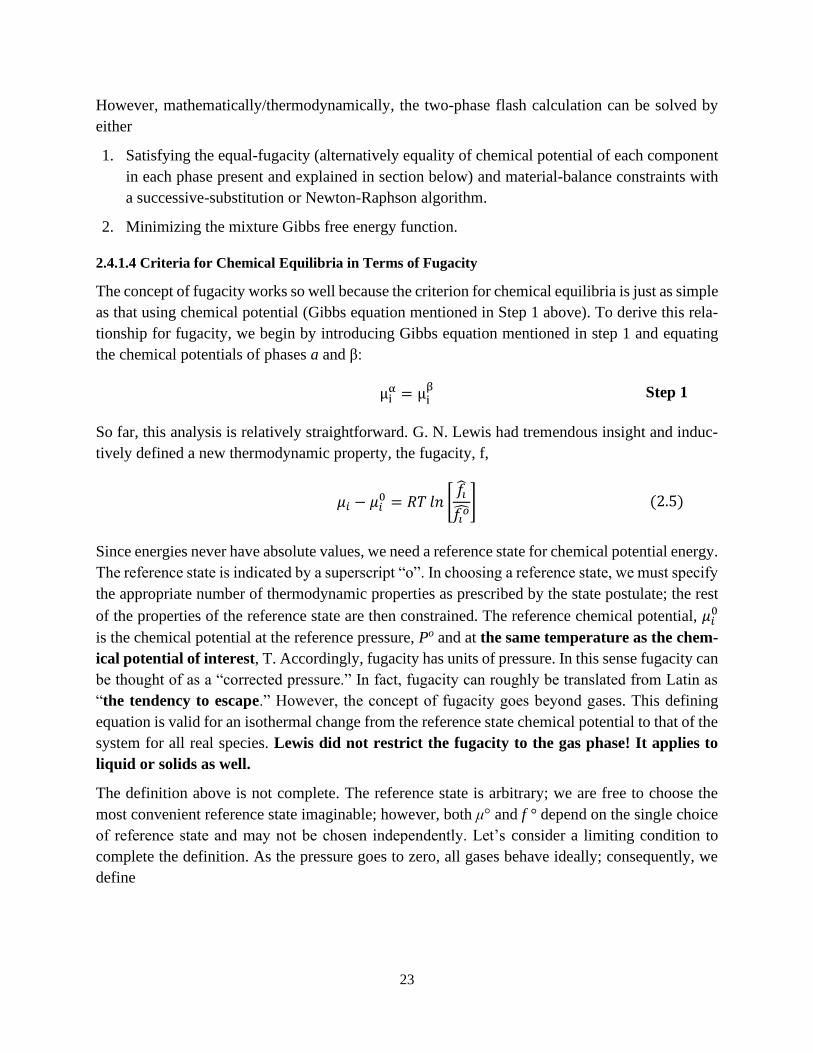
So far, this analysis is relatively straightforward. G. N. Lewis had tremendous insight and induc-

tively defined a new thermodynamic property, the fugacity, f,

Since energies never have absolute values, we need a reference state for chemical potential energy.

The reference state is indicated by a superscript “o”. In choosing a reference state, we must specify

the appropriate number of thermodynamic properties as prescribed by the state postulate; the rest

of the properties of the reference state are then constrained. The reference chemical potential, 𝜇𝑖0

is the chemical potential at the reference pressure, Po and at the same temperature as the chem-

ical potential of interest, T. Accordingly, fugacity has units of pressure. In this sense fugacity can

be thought of as a “corrected pressure.” In fact, fugacity can roughly be translated from Latin as

“the tendency to escape.” However, the concept of fugacity goes beyond gases. This defining

equation is valid for an isothermal change from the reference state chemical potential to that of the

system for all real species. Lewis did not restrict the fugacity to the gas phase! It applies to

liquid or solids as well.

The definition above is not complete. The reference state is arbitrary; we are free to choose the

most convenient reference state imaginable; however, both μ° and f ° depend on the single choice

of reference state and may not be chosen independently. Let’s consider a limiting condition to

complete the definition. As the pressure goes to zero, all gases behave ideally; consequently, we

define

μiα = μi

β Step 1

𝜇𝑖 − 𝜇𝑖0 = 𝑅𝑇 𝑙𝑛 [

𝑓�̂�

𝑓𝑖�̂�] (2.5)

24

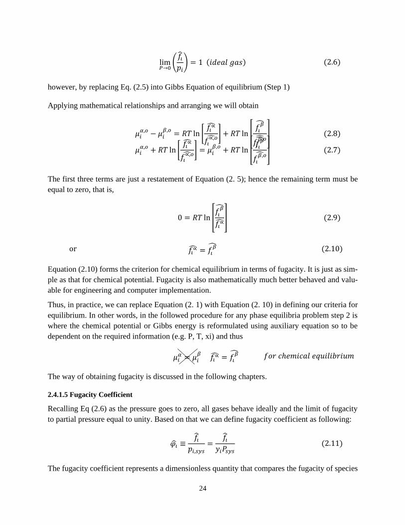
however, by replacing Eq. (2.5) into Gibbs Equation of equilibrium (Step 1)

Applying mathematical relationships and arranging we will obtain

The first three terms are just a restatement of Equation (2. 5); hence the remaining term must be

equal to zero, that is,

Equation (2.10) forms the criterion for chemical equilibrium in terms of fugacity. It is just as sim-

ple as that for chemical potential. Fugacity is also mathematically much better behaved and valu-

able for engineering and computer implementation.

Thus, in practice, we can replace Equation (2. 1) with Equation (2. 10) in defining our criteria for

equilibrium. In other words, in the followed procedure for any phase equilibria problem step 2 is

where the chemical potential or Gibbs energy is reformulated using auxiliary equation so to be

dependent on the required information (e.g. P, T, xi) and thus

The way of obtaining fugacity is discussed in the following chapters.

2.4.1.5 Fugacity Coefficient

Recalling Eq (2.6) as the pressure goes to zero, all gases behave ideally and the limit of fugacity

to partial pressure equal to unity. Based on that we can define fugacity coefficient as following:

The fugacity coefficient represents a dimensionless quantity that compares the fugacity of species

lim𝑃→0

(𝑓�̂�𝑝𝑖

) = 1 (𝑖𝑑𝑒𝑎𝑙 𝑔𝑎𝑠) (2.6)

𝜇𝑖𝛼,𝑜 + 𝑅𝑇 ln [

𝑓𝑖∝̂

𝑓𝑖∝,�̂�

] = 𝜇𝑖𝛽,𝑜

+ 𝑅𝑇 ln [𝑓𝑖

�̂�

𝑓𝑖𝛽,�̂�

] (2.7)

𝜇𝑖𝛼,𝑜 − 𝜇𝑖

𝛽,𝑜= 𝑅𝑇 ln [

𝑓𝑖∝̂

𝑓𝑖∝,�̂�

] + 𝑅𝑇 ln [𝑓𝑖

�̂�

𝑓𝑖𝛽,�̂�

] (2.8)

0 = 𝑅𝑇 ln [𝑓𝑖

�̂�

𝑓𝑖∝̂] (2.9)

or 𝑓𝑖∝̂ = 𝑓𝑖�̂�

(2.10)

𝜇𝑖𝛼 = 𝜇𝑖

𝛽 𝑓𝑖∝̂ = 𝑓𝑖

�̂� 𝑓𝑜𝑟 𝑐ℎ𝑒𝑚𝑖𝑐𝑎𝑙 𝑒𝑞𝑢𝑖𝑙𝑖𝑏𝑟𝑖𝑢𝑚

𝜑�̂� ≡𝑓�̂�

𝑝𝑖,𝑠𝑦𝑠=

𝑓�̂�𝑦𝑖𝑃𝑠𝑦𝑠

(2.11)

25

i to the partial pressure species i would have in the system as an ideal gas. A fugacity coefficient

of one represents the case where attractive and repulsive forces balance and is usually indicative

of an ideal gas. If 𝜑𝑖< 1, the corrected pressure, or “tendency to escape,” is less than that for an

ideal gas. In this case, attractive forces dominate the system behavior. Conversely, when 𝜑𝑖 > 1,

repulsive forces are stronger. Warning: We define the fugacity coefficient relative to the system

partial pressure, not the partial pressure of the reference state. A common mistake is to use the

wrong pressure here.

2.4.1.6 Equilibrium and Equilibrium Ratios (Ki)

Consider a liquid-vapor in equilibrium. As we have discussed previously, a condition for equilib-

rium is that the chemical potential of each component in both phases are equal, thus:

This is, for a system to be in equilibrium, the fugacity of each component in each of the phases

must be equal as well. The fugacity of a component in a mixture can be expressed in terms of the

fugacity coefficient. Therefore, the fugacity of a component in either phase can be written as:

Now considering for liquid -vapor in equilibrium 𝛽 represent the vapor phase (V) and 𝛼 the liquid

phase one (L) and introducing Eq. (2. 12) and Eq. (2. 13) into fugacity equality condition of equi-

librium

This equilibrium condition can be written in terms of the equilibrium ratio 𝑲𝒊 to have:

2.4.1.7 Mass Balance

For a system with C components and π possible phases, the following mass balance must be satis-

fied for each component:

μiα = μi

β

𝑓𝑖∝̂ = 𝑓𝑖�̂�

𝑓𝑖𝛽

= 𝑦𝑖∅𝑖𝛽𝑃 (2.12)

and 𝑓𝑖𝛼 = 𝑥𝑖∅𝑖

𝛼𝑃 (2.13)

𝑦𝑖∅𝑖𝑉𝑃 = 𝑥𝑖∅𝑖

𝐿𝑃 (2.14)

𝐾𝑖 =𝑦𝑖

𝑥𝑖=

∅𝑖𝐿

∅𝑖𝑉 (2.15)

26

where ak is the normalized molar amount of phase k (i.e. phase fraction) and xik is the mole fraction

of component i in phase k. We can define a reference phase, r, with the requirement that it must be

present at equilibrium (e.g. Liquid hydrocarbon in VLE). In this case, Equation 2.1 can be written

as

the following constraints are imposed on Eq. (2. 17)

Equation (2. 17), with constraints (2. 18a) which state that all mass fractions of phases present sum

up to unity and (2. 18b) a constraint that mole fractions in 𝑘 phase must satisfy by add up to unity

also, these two constraints are necessary for a closed system in order for the mass balance to be

respected. After defining the concept of material balance and necessary constraint, let’s implement

that for VLE problem which is typical in petroleum engineering.

As we have defined before 𝛽 represent the vapor phase (V) and 𝛼 the liquid phase one (L). Addi-

tionally,𝑥𝑖, 𝑦𝑖 , 𝑧𝑖 mole fraction in liquid vapor phase and original feed respectively. Defining

Liquid hydrocarbon as a reference phase since we know that liquid phase is present at equilibrium

and implementing Equation 2. 17 give us:

implying constraint 2.18 𝛼 + 𝛽 = 1 and replacing 𝛼 by 1- 𝛽 give:

∑ 𝛼𝑘 𝑥𝑖𝑘 = 𝑧𝑖

𝜋

𝑘=1

(2.16)

𝑖 = 1,… , 𝐶

𝑎𝑟𝑥𝑖𝑟 + ∑ ∝𝑘 𝑥𝑖𝑘

𝜋

𝑘=1𝑘≠𝑟

= 𝑧𝑖 (2. 17)

𝑖 = 1,… , 𝐶

𝛼𝑟 = 1 − ∑ ∝𝑘

𝜋

𝑘=1𝑘≠𝑟

(2.18a)

& ∑𝑥𝑖𝑘 = 1

𝑐

𝑖=1

(2.18b)

𝑘 = 1,… , 𝜋

𝑥𝑖𝛼 + 𝑦𝑖𝛽 = 𝑧𝑖 𝑖 = 1,… , 𝐶 (2.19)

27

Figure 6 Two phase system

now by introducing equilibrium ratio Eq. (2. 15) into Eq. (2. 20)

now solving for 𝑦𝑖

Applying constraint (2.18)

This equation is important for us; we call it an objective function because we can use it as the

starting point for solving the vapor-liquid equilibrium problems we have posed. However, as you

may be thinking right now, this is not the only choice that we have for an objective function. In

fact, we may obtain another objective function if we repeat the previous steps, while solving in-

stead for 𝑥𝑖 and having

Both (2. 23) and (2. 24) are plausible objective functions. Either of them allows us to solve the

𝑥𝑖(1 − 𝛽 ) + 𝑦𝑖𝛽 = 𝑧𝑖 (2.20)

𝑦𝑖𝛽 +𝑦𝑖

𝐾𝑖(1 − 𝛽) = 𝑧𝑖 (2.21)

𝑦𝑖 =𝑧𝑖 𝐾𝑖

1 + 𝛽(𝐾𝑖 − 1) (2.22)

∑𝑧𝑖𝐾𝑖

1 + 𝛽(𝐾𝑖 − 1)

𝐶

𝑖=1

= 1 (2.23)

∑𝑧𝑖

1 + 𝛽(𝐾𝑖 − 1)

𝐶

𝑖=1

= 1 (2.24)

28

flash problem that we are dealing with. The variables that make up both equations are:

C =Number of components

𝑧𝑖= Overall composition (Feed composition)

𝐾𝑖= Equilibrium ratios of each of the components of the mixture

𝛽 =Vapor fraction in the system.

What is it that we are looking for? Go back and look at the types of VLE problems that we would

like to solve, as we presented them in the previous section. If we are interested in solving the flash

problem, we want to know how much liquid and gas we will have inside the flash equilibrium cell.

This is, given a liquid-vapor mixture of composition 𝑧𝑖and C number of components, what percent

of the total number of moles is liquid, and what percent is vapor? How do we split it? In this case,

we would like to come up with a value for 𝛼 and 𝛽 respectively.

Both Eq.s (2. 23) and (2. 24) give us the answer for these questions taking into consideration that

we do have “Known 𝐾𝑖”, but keep in mind that 𝐾𝑖 are functions of the pressure, temperature, and

composition of the system.

For the time being, let us assume that we do have valuable Ki’s. Two questions remain unanswered:

1. First, is it “better” to solve the problem using Eq. (2. 23) or (2. 24)?

2. Second, how do we solve for𝛽? For a complex mixture of many components, “𝛽” cannot be

calculated explicitly.

We will address both of these questions in the next sections.

2.4.1.8 Analysis of the Objective Functions and the Need for Rachford-Rice Equation

In a previous module we derived two different objective functions (Eq. 2. 23 & 2.2 4) for the

purpose of solving the flash equilibrium problem. These equations arise from simple mole balances

and the concept of equilibrium ratios. In addition, we have assumed that 𝐾𝑖′𝑠 are obtained where

the only unknown will be 𝛽 or molar fraction of one phase while the molar fraction for the other

phase is calculated from complimentary equation that state all molar fraction sum up to unity.

Once we are able to solve for molar fraction of the phase, by implementing Eq. 2. 22 or similar

equation for𝑥𝑖. In other words, phase compositions of the present phases at equilibrium can be

solved. However, one question that raised up in section before that how we can solve for molar

fraction where we can notice that both equations are nonlinear in molar phase fraction. This mean

that we cannot solve the molar phase fraction explicitly as function of other variable where iterative

techniques are required such as Newton-Raphson approach. A distinctive characteristic of any

Newton-Raphson procedure is that the success of the procedure depends greatly upon the choice

of the initial guess for the variable considered. In fact, it is very commonly said that for Newton-

Raphson to converge, the initial guess must be as close as possible to the real solution. This ‘ill-

29

nesses become worse when dealing with non-monotonic functions. In a monotonic function, de-

rivatives at every point are always of the same sign where the function either increases or decreases

monotonically. For Newton-Raphson, this means that there are neither valleys nor peaks that could

lead the procedure to false solutions. If we apply Newton-Raphson to a monotonic and everywhere-

continuous function, the success of the procedure is not strongly dependent on the initial guess. In

fact, if we apply Newton-Raphson to a monotonic function that is continuous at every single point

of the domain as well, it does not matter at all where you start: you will always find the solution.

It might take time to achieve convergence, but you will be able to converge to a unique solution.

Based on these facts and that neither Eq. 2. 23 nor 2. 24 are not monotonic which make the con-

vergence to be harder to be achieved and having a correct solution. (Rachford (1952)) Solved this

problem by defining a new monotonic objective function so to simplify the iteration procedure

using both Eq. 2. 23 & 2.24 but in a different form respectively as following where ∝𝑔molar phase

fraction of vapor is phase

where the combination yield

Eq.(2.28) is the Rachford-Rice Equation. In order to demonstrate the monotonic behavior of this

equation, the first derivative of Rachford-Rice show that the outcome of this summation will be

always positive due to the square’s presence both in numerator and denominator and that overall

composition 𝑧𝑖 is always positive

We have already answered to the questions that have raised up in the last section where one ques-

tion remains unanswered:

In the previous development, we made one crucial assumption. We assumed that, somehow, we

knew all the equilibrium ratios. The fact is, however, that we usually don’t. If we do not know all

𝐹𝑦(∝𝑔) = ∑𝑧𝑖𝐾𝑖

1 +∝𝑔 (𝐾𝑖 − 1)

𝐶

𝑖=1

− 1 = 0 (2.25)

𝐹𝑥(∝𝑔) = ∑𝑧𝑖

1 +∝𝑔 (𝐾𝑖 − 1)

𝑛

𝑖=1

− 1 = 0 (2.26)

𝐹𝑠 = 𝐹𝑦(∝𝑔) − 𝐹𝑥(∝𝑔) (2.27)

𝐹(∝𝑔) = ∑𝑧𝑖(𝐾𝑖 − 1)

1 +∝𝑔 (𝐾𝑖 − 1)

𝑛

𝑖=1

= 0 (2.28)

𝐹′(∝𝑔) = ∑𝑧𝑖(𝐾𝑖 − 1)2

{1 +∝𝑔 (𝐾𝑖 − 1)}2

𝑛

𝑖=1

= 0 (2.29)

30

equilibrium ratios, then all of the previous discussions are meaningless. So far, the only conclusion

we can draw is that if that we should find a way to know𝐾𝑖’s so that the VLE problem is solva-

ble.by doing that we conclude the discussion about VL equilibria (Two phase equilibria).

2.4.1.9 Obtaining Ki’s Equilibrium Ratios

The Ki value of each component in a real hydrocarbon mixture is a function of the pressure, tem-

perature and also of the composition of each of the phases. Since the compositions of the phases

are not known beforehand, equilibrium constants are not known, either. If they were known, the

VLE calculation would be performed in a straightforward manner.

Nevertheless, the good news is that sometimes Ki’s are fairly independent of the phase’s composi-

tion. This is true at pressure and temperature conditions away from the critical point of the mixture.

Therefore, numerous correlations have been developed throughout the years to estimate the values

of Ki for each hydrocarbon component as a function of the pressure and temperature of the system.

The values produced from this correlation are called Ideal Ki’s and can be used for first estimation

in the iteration procedure after that and based on the results obtained, they can be updated using

different iterative procedure such as Successive substitution (SS) or accelerated successive substi-

tution (aSS) in some cases especially near to the critical point and sometimes Newton-Raphson.

A very popular empirical correlation that is very often used in the petroleum and natural gas in-

dustry is Wilson’s empirical correlation for initializing the algorithm or as initial guess is as fol-

lowing (M. Michelsen (1982a))

𝑇𝑐𝑖 is critical temperature, in ºR or K, 𝑃𝑐𝑖, critical pressure, in psi, kPa or bar, 𝜔𝑖 is the acentric

factor, P is the system pressure, in psi, kPa or bar, T is the system temperature, in ºR or K. (P and

Pc, T and Tc must be in the same units.) This correlation can be considered accurate at low and

moderate pressure, up to about 3.5 MPa (500 psia) where the K-values are assumed to be inde-

pendent of composition “ideal 𝐾𝑖′𝑠”.

2.4.1.10 Summary

In previous sections we have discussed that all system at equilibrium regardless of how many

phases they will be present can be solved and formulated using the Three step application proce-

dure. In fact, any engineering problem can be solved in the same way. We start by describing the

system that we want to solve by finding an equation that describe the system of interest and may

help to formulate the problem mathematically. In our case (phase equilibria problem) classical

thermodynamic provide the mathematical language to formulate and solve the problem. For this

purpose, we described the problem as function of chemical potential and free energy where we

reduced this condition so to be valuable for engineering purposes. This step has been achieved

𝐾𝑖 =𝑃𝑐𝑖

𝑃𝑒𝑥𝑝 [5.373(𝜔𝑖) (1 −

𝑇𝑐𝑖

𝑇)] (2.30)

31

using some auxiliary function such as fugacity and fugacity coefficient in this case (VLE) while

in other cases like hydrate the need of activity coefficient is necessary in some cases. However,

the procedure that should be followed so to solve the problem must have a physical meaning to

what is actually present in the system in the real world. Based on that we defined Ki’s ratios where

it has been merged with mass balance calculations later on. The result of which two non- mono-

tonic objective function can be used to solve the problem.

Due to the nature of the phase equilibria problem and available data it has been concluded that

iterative technique is necessary such as Newton-Raphson. After careful analysis of the objective

functions and iterative procedure chosen so that to obtain a valuable and correct result the need of

a monotonic objective function appeared. Thanks to (Rachford (1952)) and solution provided for

this problem a new objective function has be found. Finally, we concluded that obtaining a math-

ematical solution for phase equilibria problem can be achieved under the circumstances that equi-

librium ratio can be obtained. Where Ki’s are value of each component in a real hydrocarbon

mixture is a function of the pressure, temperature and also of the composition of each of the phases

which are not known in advance we concluded that the well-known correlation in oil and gas

industry Wilson’s empirical correlation can be used as a first estimate for initiating the algorithm.

However, we should keep in mind that all of this discussion and the procedure followed is made

under the assumption that the system will split, and two-phase system will be formed. This obstacle

will be discussed in the followed sections of this chapter. At the end phase equilibria problem is

summarized and presented in the algorithm below taking into consideration that relationship for

fugacity and fugacity coefficient with T, P and phase composition are present in our hand (will be

discussed later).

32

2.4.1.11 Algorithm

Figure 7 Typical Algorithm for Two phase flash system (produced in this work).

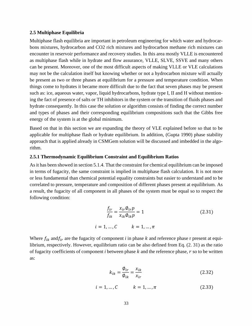
33

2.5 Multiphase Equilibria

Multiphase flash equilibria are important in petroleum engineering for which water and hydrocar-

bons mixtures, hydrocarbon and CO2 rich mixtures and hydrocarbon methane rich mixtures can

encounter in reservoir performance and recovery studies. In this area mostly VLLE is encountered

as multiphase flash while in hydrate and flow assurance, VLLE, SLVE, SSVE and many others

can be present. Moreover, one of the most difficult aspects of making VLLE or VLE calculations

may not be the calculation itself but knowing whether or not a hydrocarbon mixture will actually

be present as two or three phases at equilibrium for a pressure and temperature condition. When

things come to hydrates it became more difficult due to the fact that seven phases may be present

such as: ice, aqueous water, vapor, liquid hydrocarbons, hydrate type I, II and H without mention-

ing the fact of presence of salts or TH inhibitors in the system or the transition of fluids phases and

hydrate consequently. In this case the solution or algorithm consists of finding the correct number

and types of phases and their corresponding equilibrium compositions such that the Gibbs free

energy of the system is at the global minimum.

Based on that in this section we are expanding the theory of VLE explained before so that to be

applicable for multiphase flash or hydrate equilibrium. In addition, (Gupta 1990) phase stability

approach that is applied already in CSMGem solution will be discussed and imbedded in the algo-

rithm.

2.5.1 Thermodynamic Equilibrium Constraint and Equilibrium Ratios

As it has been showed in section 5.1.4. That the constraint for chemical equilibrium can be imposed

in terms of fugacity, the same constraint is implied in multiphase flash calculation. It is not more

or less fundamental than chemical potential equality constraints but easier to understand and to be

correlated to pressure, temperature and composition of different phases present at equilibrium. As

a result, the fugacity of all component in all phases of the system must be equal so to respect the

following condition:

Where 𝑓𝑖𝑘 and𝑓𝑖𝑟 are the fugacity of component i in phase 𝑘 and reference phase r present at equi-

librium, respectively. However, equilibrium ratio can be also defined from Eq. (2. 31) as the ratio

of fugacity coefficients of component i between phase 𝑘 and the reference phase, 𝑟 so to be written

as:

𝑓𝑖𝑟𝑓𝑖𝑘

=𝑥𝑖𝑟∅𝑖𝑟𝑝

𝑥𝑖𝑘∅𝑖𝑘𝑝= 1 (2.31)

𝑖 = 1,… , 𝐶 𝑘 = 1,… , 𝜋

𝑘𝑖𝑘 =∅𝑖𝑟

∅𝑖𝑘=

𝑥𝑖𝑘

𝑥𝑖𝑟 (2.32)

𝑖 = 1,… , 𝐶 𝑘 = 1,… , 𝜋 (2.33)

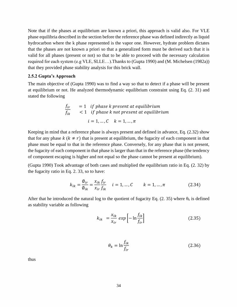
34

Note that if the phases at equilibrium are known a priori, this approach is valid also. For VLE

phase equilibria described in the section before the reference phase was defined indirectly as liquid

hydrocarbon where the k phase represented is the vapor one. However, hydrate problem dictates

that the phases are not known a priori so that a generalized form must be derived such that it is

valid for all phases (present or not) so that to be able to proceed with the necessary calculation

required for each system (e.g VLE, SLLE…).Thanks to (Gupta 1990) and (M. Michelsen (1982a))

that they provided phase stability analysis for this brick wall.

2.5.2 Gupta’s Approach

The main objective of (Gupta 1990) was to find a way so that to detect if a phase will be present

at equilibrium or not. He analyzed thermodynamic equilibrium constraint using Eq. (2. 31) and

stated the following

Keeping in mind that a reference phase is always present and defined in advance, Eq. (2.32) show

that for any phase 𝑘 (𝑘 ≠ 𝑟) that is present at equilibrium, the fugacity of each component in that

phase must be equal to that in the reference phase. Conversely, for any phase that is not present,

the fugacity of each component in that phase is larger than that in the reference phase (the tendency

of component escaping is higher and not equal so the phase cannot be present at equilibrium).

(Gupta 1990) Took advantage of both cases and multiplied the equilibrium ratio in Eq. (2. 32) by

the fugacity ratio in Eq. 2. 33, so to have:

After that he introduced the natural log to the quotient of fugacity Eq. (2. 35) where θk is defined

as stability variable as following

thus

𝑓𝑖𝑟𝑓𝑖𝑘

= 1 𝑖𝑓 𝑝ℎ𝑎𝑠𝑒 𝑘 𝑝𝑟𝑒𝑠𝑒𝑛𝑡 𝑎𝑡 𝑒𝑞𝑢𝑖𝑙𝑖𝑏𝑟𝑖𝑢𝑚 < 1 𝑖𝑓 𝑝ℎ𝑎𝑠𝑒 𝑘 𝑛𝑜𝑡 𝑝𝑟𝑒𝑠𝑒𝑛𝑡 𝑎𝑡 𝑒𝑞𝑢𝑖𝑙𝑖𝑏𝑟𝑖𝑢𝑚

𝑖 = 1,… , 𝐶 𝑘 = 1,… , 𝜋

𝑘𝑖𝑘 =∅𝑖𝑟

∅𝑖𝑘=

𝑥𝑖𝑘

𝑥𝑖𝑟

𝑓𝑖𝑟𝑓𝑖𝑘

𝑖 = 1, … , 𝐶 𝑘 = 1,… , 𝜋 (2.34)

𝑘𝑖𝑘 =𝑥𝑖𝑘

𝑥𝑖𝑟 𝑒𝑥𝑝 [− ln

𝑓𝑖𝑘𝑓𝑖𝑟

] (2.35)

𝜃𝑘 = ln𝑓𝑖𝑘𝑓𝑖𝑟

(2.36)

35

rewriting Eq. 2. 37 in terms of the mole fraction ratio as

Eq. 2.38 can be applied for all phases regardless of the phase’s presence in the system at equilib-

rium. (Gupta 1990) Showed that defining the mole fraction ratio in this manner is equivalent to

minimizing the Gibbs energy of the system conditional to

2.5.3 Mass Balance (Rachford-Rice Extension and Gupta’s Parameter Implementation)

In section 5.1.7 we have shown how to derive mole fraction and two objective function from sim-

ple mole balances and equilibrium ratios. In this way these equations can be expanded in the same

basis matter so to be valid for multiphase systems. However, in this section we are showing the

extended equations for multiphase flash calculation including Gupta’s parameters for stability

analysis purpose. Note that in VLE section we have defined indirectly that the reference phase is

liquid hydrocarbon one while in multiphase flash the following expression for the composition of

component i in the reference phase including Gupta stability parameter is as following:

Using equation 2.38 and recognizing that 𝑘𝑖r = 1 and 𝜃𝑘=0, Equation 2.40 can be rewritten for

component i in any phase k as

By implementing constraint 2. 18b that state the summarization of all components in phase k must

be equal to unity, we get the objective function, Ik, for each phase

𝑘𝑖𝑘 =𝑥𝑖𝑘

𝑥𝑖𝑟 𝑒𝑥𝑝[−𝜃𝑘] (2.37)

𝑥𝑖𝑘

𝑥𝑖𝑟= 𝑘𝑖𝑘𝑒𝜃𝑘 𝑖 = 1,… , 𝐶 𝑘 = 1,… , 𝜋 (2.38)

𝑆𝑘 = ∝𝑘 𝜃𝑘 = 0 𝑘 = 1,… , 𝜋 (2.39)

that is, if

• ∝𝑘 > 0 then phase k is present and 𝜃𝑘 = 0

• ∝𝑘 = 0 then phase k is not present and 𝜃𝑘 ≠ 0

𝑥𝑖𝑟 =𝑧𝑖

1 + ∑ ∝𝑘 (𝑘𝑖𝑘𝑒𝜃𝑘 − 1)𝜋𝑘=1𝑘≠𝑟

𝑖 = 1, . . . , 𝐶 (2.40)

𝑥𝑖𝑘 =𝑧𝑖𝐾𝑖𝑘𝑒

𝜃𝑘

1 + ∑ ∝𝑗 (𝐾𝑖𝑗𝑒𝜃𝑗 − 1)𝜋

𝑗=1𝑗≠𝑟

𝑖 = 1,… , 𝐶 𝑘 = 1,… , 𝜋

(2.41)

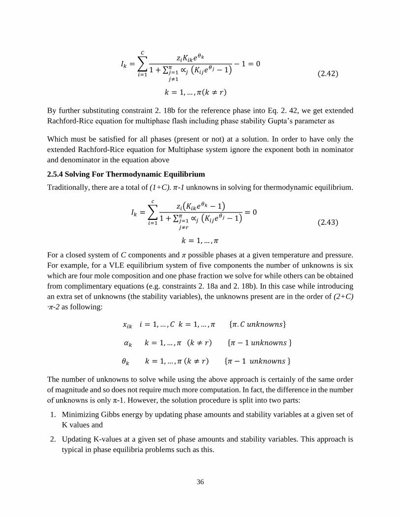
36

By further substituting constraint 2. 18b for the reference phase into Eq. 2. 42, we get extended

Rachford-Rice equation for multiphase flash including phase stability Gupta’s parameter as

Which must be satisfied for all phases (present or not) at a solution. In order to have only the

extended Rachford-Rice equation for Multiphase system ignore the exponent both in nominator

and denominator in the equation above

2.5.4 Solving For Thermodynamic Equilibrium

Traditionally, there are a total of (1+C). 𝜋-1 unknowns in solving for thermodynamic equilibrium.

For a closed system of C components and π possible phases at a given temperature and pressure.

For example, for a VLE equilibrium system of five components the number of unknowns is six

which are four mole composition and one phase fraction we solve for while others can be obtained

from complimentary equations (e.g. constraints 2. 18a and 2. 18b). In this case while introducing

an extra set of unknowns (the stability variables), the unknowns present are in the order of (2+C)

·π-2 as following:

The number of unknowns to solve while using the above approach is certainly of the same order

of magnitude and so does not require much more computation. In fact, the difference in the number

of unknowns is only π-1. However, the solution procedure is split into two parts:

1. Minimizing Gibbs energy by updating phase amounts and stability variables at a given set of

K values and

2. Updating K-values at a given set of phase amounts and stability variables. This approach is

typical in phase equilibria problems such as this.

𝐼𝑘 = ∑

𝑧𝑖𝐾𝑖𝑘𝑒𝜃𝑘

1 + ∑ ∝𝑗 (𝐾𝑖𝑗𝑒𝜃𝑗 − 1)𝜋

𝑗=1𝑗≠1

𝐶

𝑖=1

− 1 = 0

𝑘 = 1,… , 𝜋(𝑘 ≠ 𝑟)

(2.42)

𝐼𝑘 = ∑𝑧𝑖(𝐾𝑖𝑘𝑒

𝜃𝑘 − 1)

1 + ∑ ∝𝑗 (𝐾𝑖𝑗𝑒𝜃𝑗 − 1)𝜋

𝑗=1𝑗≠𝑟

𝑐

𝑖=1

= 0

𝑘 = 1,… , 𝜋

(2.43)

𝑥𝑖𝑘 𝑖 = 1,… , 𝐶 𝑘 = 1,… , 𝜋 {𝜋. 𝐶 𝑢𝑛𝑘𝑛𝑜𝑤𝑛𝑠}

𝛼𝑘 𝑘 = 1,… , 𝜋 (𝑘 ≠ 𝑟) {𝜋 − 1 𝑢𝑛𝑘𝑛𝑜𝑤𝑛𝑠 }

𝜃𝑘 𝑘 = 1, … , 𝜋 (𝑘 ≠ 𝑟) {𝜋 − 1 𝑢𝑛𝑘𝑛𝑜𝑤𝑛𝑠 }

37

2.5.4.1 Minimizing Gibbs Energy (At A Given Phase Fractions/Compositions)

Different iterative procedure can be used so to minimize the Gibbs energy of the system at a given

set of K-values. The one that is mostly implied for such problems is Newton-Raphson. Using ex-

tended Rachford-Rice equation for multiphase with Gupta’s constraint, convergency can be

achieved as long as fugacity coefficients are not strong functions of composition. This is certainly

the case for the fluid phases such as vapor and liquid hydrocarbon in VLE near to or at the critical

point but is not necessarily true for the aqueous and hydrate phases in our case here.

In order to implement or to use the Newton procedure, the derivatives of Equation 2. 43 are needed

with respect to each unknown variable 𝛼𝑗 and 𝜃𝑗 . In addition, the simple derivatives of Equation

2. 39.

The derivatives of Eq. 2. 43 with respect to each variable are as following:

However, we have just mentioned in this work Multiphase flash equilibria problem but taking into

consideration solving for temperature or pressure as it is the case in VLE other problem mentioned

in the specific section in which a given phase forms having molar fraction phase in the magnitude

of Ꜫ, the following derivative of Equation 2. 43 is given:

However, the derivative of the K-values with respect to T or P is still needed. It is assumed, for

this derivative, that the K-values are constant in composition and change only with temperature

and pressure. Due to the complexity of the equations of state used, numerical approximation can

be used (e.g. forward). Going back to main task Multiphase flash and stability the Newton method

gives a correction to the phase amounts and stability variables based on the gradient of the Gibbs

energy at the given set of K-values. Due to the highly non-ideal behavior of the hydrate phases,

some restriction may be needed so to avoid an ad rapt change set in the variables that we are

iterating for.

𝜕𝐼𝑘𝜕𝛼𝑗

= −∑𝑧𝑖(𝐾𝑖𝑘𝑒

𝜃𝑘 − 1)(𝐾𝑖𝑗𝑒𝜃𝑗 − 1)

(1 + ∑ ∝𝑚 (𝐾𝑖𝑚𝑒𝜃𝑚 − 1)𝜋𝑚=1𝑚≠𝑟

)2

𝑐

𝑖=1

𝑘 = 1,… , 𝜋 (𝑘 ≠ 𝑟)

𝑗 = 1,… , 𝜋 (𝑗 ≠ 𝑟)

(2.44)

and 𝜕𝐼𝑘𝜕𝜃𝑗

= −∑𝑧𝑖(𝐾𝑖𝑘𝑒

𝜃𝑘 − 1) ∝𝑗 𝐾𝑖𝑗𝑒𝜃𝑗

(1 + ∑ ∝𝑚 (𝐾𝑖𝑚𝑒𝜃𝑚 − 1)𝜋𝑚=1𝑚≠𝑟

)2

𝑐

𝑖=1

𝑘 = 1,… , 𝜋 (𝑘 ≠ 𝑟)

𝑗 = 1, … , 𝜋 (𝑗 ≠ 𝑟)

(2.45)

𝜕𝐼𝑘𝜕𝑃

=𝜕𝐼𝑘𝜕𝑇

= ∑𝑥𝑖𝑟

𝑐

𝑖=1

[

𝜕𝐾𝑖𝑘

𝜕𝑃 𝑜𝑟 𝜕𝑇 𝑒𝜃𝑚 −

(𝐾𝑖𝑘𝑒𝜃𝑘 − 1)∑ ∝𝑗

𝜋𝑗=1𝑗≠𝑟

𝜕𝐾𝑖𝑗

𝜕𝑃 𝑜𝑟 𝜕𝑇 𝑒𝜃𝑗

(1 + ∑ ∝𝑗𝜋𝑗=1𝑗≠𝑟

(𝐾𝑖𝑗𝑒𝜃𝑗 − 1))

]

(2.46)

38

2.5.4.2 Updating K-Values and Composition at A Given Gibbs Energy

After that Gibbs energy is minimized at a given set of K-values, the K’s need to be updated together

with composition. Equation 2. 41 is used to update the composition of each phase. With the new

composition, the fugacity coefficients are calculated to get the new set of K-values. Successive

substitution or accelerated successive substitution iteration of the composition can be used to

achieve convergence. However, due to the highly non-ideal behavior of the hydrate phases, equa-

tion mentioned before can be replaced with fractional occupancy of guest molecule in hydrate

cavities (will be explained after) to update the composition.

2.5.5 Ki’s Values for Hydrate Problem

In order to initialize Gibbs energy minimization algorithm explained in the last sections, Ki series

values for (𝜋-1) number of phases need to be defined. In the same case of VLE where ideal K

values (composition independent) set can defined for vapor/liquid hydrocarbon using Wilson em-

pirical correlation as first estimate, in hydrate also we are seeking expressions and empirical cor-

relations for distribution of components between each phase with respect to the reference phase

that is always present at equilibrium. This expressions or approaches should be at least sufficient

as a starting value in the algorithm. Before doing so, let’s have a look on hydrate phase diagram

so to have clear understanding of what phases can be present first.

Based on P-T hydrate diagram, the phases that can be present at equilibrium are ice, liquid water,

liquid hydrocarbon, vapor and hydrate. Note that hydrates can form different structures (I, II and

H) as well where several researchers have developed expressions for distribution of guest mole-

cules between the vapor and hydrate phase, some of them produced K-values independent on hy-

drate structure while some others (S.L.Mann 1989) developed K-values structure dependent. How-

ever, the most common set of K-values implemented these days and the different software used in

this work (e.g. CSMGem, HydraFLASH) are structure dependents ones. Additionally, to that in

case of salts and thermodynamic inhibitors presence in the system additional set of Ki’s are re-

quired (e.g. Salts in the aqueous phases).

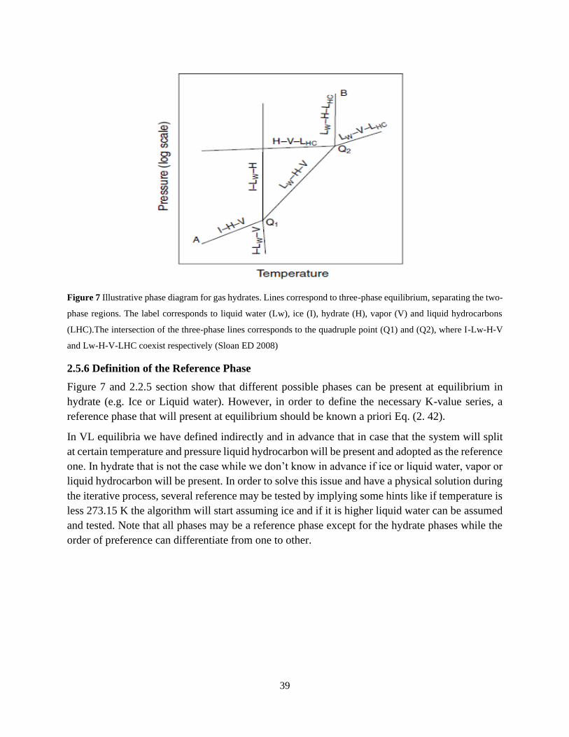
39

Figure 7 Illustrative phase diagram for gas hydrates. Lines correspond to three-phase equilibrium, separating the two-

phase regions. The label corresponds to liquid water (Lw), ice (I), hydrate (H), vapor (V) and liquid hydrocarbons

(LHC).The intersection of the three-phase lines corresponds to the quadruple point (Q1) and (Q2), where I-Lw-H-V

and Lw-H-V-LHC coexist respectively (Sloan ED 2008)

2.5.6 Definition of the Reference Phase

Figure 7 and 2.2.5 section show that different possible phases can be present at equilibrium in

hydrate (e.g. Ice or Liquid water). However, in order to define the necessary K-value series, a

reference phase that will present at equilibrium should be known a priori Eq. (2. 42).

In VL equilibria we have defined indirectly and in advance that in case that the system will split

at certain temperature and pressure liquid hydrocarbon will be present and adopted as the reference

one. In hydrate that is not the case while we don’t know in advance if ice or liquid water, vapor or

liquid hydrocarbon will be present. In order to solve this issue and have a physical solution during

the iterative process, several reference may be tested by implying some hints like if temperature is

less 273.15 K the algorithm will start assuming ice and if it is higher liquid water can be assumed

and tested. Note that all phases may be a reference phase except for the hydrate phases while the

order of preference can differentiate from one to other.

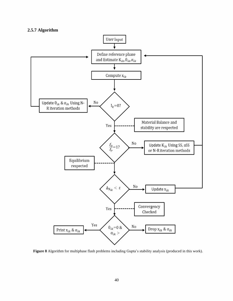
40

2.5.7 Algorithm

Figure 8 Algorithm for multiphase flash problems including Gupta’s stability analysis (produced in this work).

41

Chapter 3

3 Cubic Plus Association Eos

In Chapter 2 we have explained the concept of a flash equilibria problem for Two (VLE) and

Multiphase flash systems. In addition, we have described the chemical equilibrium using fugacity

and fugacity coefficient as auxiliary functions instead of abstract chemical equilibrium while we

didn’t mention how these parameters can be calculated or correlated with the intensive properties

of our interest. However, values of this function can be obtained in several way (e.g. Charts, Cor-

relations etc.). One of these ways is using an EoS. Refereeing to that, for petroleum and reservoir

engineers most important EoSs are the cubic ones (e.g. SRK, PR) which perform very well for

simple gases and hydrocarbon mixtures. These equations fail to produce satisfactory results for

more complex fluids such as polar solvents, electrolytes, heavy petroleum residual fluids like as-

phaltenes, polymers, and surface-active agents wherein either more sophisticated molecular inter-

actions or more complicated molecular structure and characteristics contribute to the microscopic

and macroscopic fluid properties encountered in hydrate such as water , inhibitors, alcohols. How-

ever, the key to model macroscopic properties of a fluid is the ability to describe microscopic

properties so to account for intermolecular and intermolecular interactions of the real complex

fluids. Based on that, hydrates calculations show the need for an equation of state that cover all

obstacles mentioned before so to ensure a achieving a correct solution of the problem. Thanks to

(Georgios M. Kontogeorgis 2006) who provided such equation known as CPA EoS which stands

for Cubic Plus Association equation of state. This equation is a combination of SRK or PR equa-

tions of state and association term of the SAFT/Wertheim theory. Therefore, the equation of CPA

EoS has two parts, the non-association term and association term. The development of CPA started

in 1995 as a research project funded by Shell (Amsterdam) and the model was first published in

1996. Since then, it has been successfully applied to a variety of complex phase equilibria includ-

ing mixtures containing alcohols, glycols, water and hydrocarbon.

In this chapter we will describe the CPA EoS that started gaining more attention in the last decade

in flow assurance field. Nowadays it represents the most accurate model in thermodynamic mod-

elling of hydrates. CPA EoS is used in four approaches tested in this work implemented in two

well-known software for predicting hydrate dissociation pressure and temperature in the today’s

market such as Hydra Flash (Hydra Fact company/Heriot-Watt University) and Multiphase Flash

(KBC/Schlumberger). In order to have a full understood of the equation and how it functions SAFT

model also will be discussed briefly.

3.1 Introduction

(Chapman W.G. (1990)) Proposed an equation of state by applying the Wertheim thermodynamic

perturbation theory referred as SAFT, an acronym for Statistical Association Fluid Theory. In the

original SAFT approach, molecules are considered as single (spherical particles) or multiple

chained hard-sphere segments (non-spherical molecules) with or without association sites depend-

ing on whether the molecule can form hydrogen bonding or not. Therefore, SAFT EoS is expressed

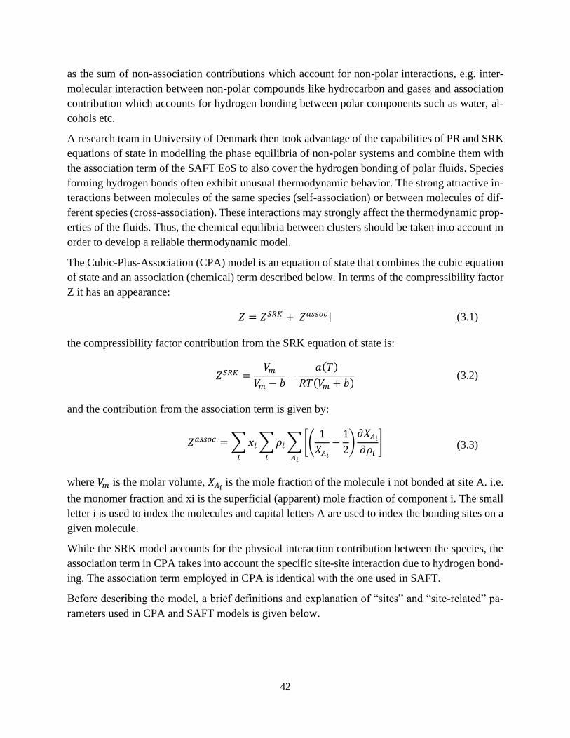
42

as the sum of non-association contributions which account for non-polar interactions, e.g. inter-

molecular interaction between non-polar compounds like hydrocarbon and gases and association

contribution which accounts for hydrogen bonding between polar components such as water, al-

cohols etc.

A research team in University of Denmark then took advantage of the capabilities of PR and SRK

equations of state in modelling the phase equilibria of non-polar systems and combine them with

the association term of the SAFT EoS to also cover the hydrogen bonding of polar fluids. Species

forming hydrogen bonds often exhibit unusual thermodynamic behavior. The strong attractive in-

teractions between molecules of the same species (self-association) or between molecules of dif-

ferent species (cross-association). These interactions may strongly affect the thermodynamic prop-

erties of the fluids. Thus, the chemical equilibria between clusters should be taken into account in

order to develop a reliable thermodynamic model.

The Cubic-Plus-Association (CPA) model is an equation of state that combines the cubic equation

of state and an association (chemical) term described below. In terms of the compressibility factor

Z it has an appearance:

the compressibility factor contribution from the SRK equation of state is:

and the contribution from the association term is given by:

where 𝑉𝑚 is the molar volume, 𝑋𝐴𝑖 is the mole fraction of the molecule i not bonded at site A. i.e.

the monomer fraction and xi is the superficial (apparent) mole fraction of component i. The small

letter i is used to index the molecules and capital letters A are used to index the bonding sites on a

given molecule.

While the SRK model accounts for the physical interaction contribution between the species, the

association term in CPA takes into account the specific site-site interaction due to hydrogen bond-

ing. The association term employed in CPA is identical with the one used in SAFT.

Before describing the model, a brief definitions and explanation of “sites” and “site-related” pa-

rameters used in CPA and SAFT models is given below.

𝑍 = 𝑍𝑆𝑅𝐾 + 𝑍𝑎𝑠𝑠𝑜𝑐| (3.1)

𝑍𝑆𝑅𝐾 =𝑉𝑚

𝑉𝑚 − 𝑏−

𝑎(𝑇)

𝑅𝑇(𝑉𝑚 + 𝑏) (3.2)

𝑍𝑎𝑠𝑠𝑜𝑐 = ∑𝑥𝑖

𝑖

∑𝜌𝑖

𝑖

∑[(1

𝑋𝐴𝑖

−1

2)

𝜕𝑋𝐴𝑖

𝜕𝜌𝑖]

𝐴𝑖

(3.3)

43

3.2 Association Energy and Volume Parameters

The key features of the hydrogen-bonds are their strength, short range and high degree of locali-

zation. In Fig. 13 it is shown a simple example of prototype spheres, or spherical segments, with

one associating site, A. Such spheres can only form an AA-bonded dimer when both distance and

orientation are favorable.

Figure 9 Model of hard spheres with a single associating site A illustrating a simple case of molecular association

due to short-distance, highly orientational, site-site attraction (Chapman W.G. (1990)).

The associating bond strength is quantified by a square-well potential, which, in turn, is character-

ized by two parameters. The parameter εΑA characterizes the association energy (well depth) and

the parameter KAA characterizes the association volume (corresponds to the well width rAA). In gen-

eral, the number of association sites on a single molecule is not constrained and they are labelled

with capital letters A, B, C, etc. Each association site is assumed to have a different interaction

with the various sites on another molecule. Examples of two associating sites molecules are given

in the Fig. 10.

Thus, for each pure component three molecular parameters, σ, ε/k and m are needed, which are the

temperature independent segment diameter in angstroms, the Lennard-Jones interaction energy in

Kelvins, and the number of segments per chain molecule, respectively. In addition, two association

parameters, association energy, εΑA/k in Kelvins and volume KAIBJ (dimensionless), for each site-

site interaction. The usual method for deriving the σ, ε and m values is to fit vapor pressure and

density data for pure components. The association parameters ε AiBj/k and K AiBj can be fitted to bulk

phase equilibrium data.

44

Figure 10 Models of hard sphere (monomer) and chain (m-mer.) molecules with two associating sites A and B; the

chain molecule represents non- spherical molecule (Chapman W.G. (1990)).

3.3 Association Term in CPA Eos

For pure components, the association term is defined in terms of the residual Helmholz energy ar

per mole, defined as

Where a and aig are the total Helmholz energy per mole and the ideal gas Helmholz energy per

mole at the same temperature and density. The residual Helmholz energy is a sum of three terms

representing contributions from different intermolecular forces: segment-segment interaction, co-

valent chain-forming bonds and site-site specific interactions among the segments, for example,

hydrogen-bonding interactions:

The extension of the CPA EoS to mixtures requires mixing rules only for the parameters of the

SRK-part, while the extension of the association term to mixtures is straightforward. The mixing

and combining rules for a and b are the classical van der Waals one.

The mixture Helmholz energy for the association term is linear with respect to mole fractions,

𝑛𝑖:

Here, A is used to index bonding sites on a given molecule and 𝑋𝐴𝑖 denotes the fraction of A- sites

on molecule i that do not form bonds with other active sites and Σ represents a sum over all asso-

ciating sites. Examples for molecules with two attractive sites and one attractive site are given as

follows (Chapman W.G. (1990))

𝑎𝑟(𝑇, 𝑉, 𝑛) = 𝑎(𝑇, 𝑉, 𝑛) − 𝑎𝑖𝑔(𝑇, 𝑉, 𝑛) (3.4)

𝑎𝑟 = 𝑎𝑠𝑒𝑔 + 𝑎𝑐ℎ𝑎𝑖𝑛 + 𝑎𝑎𝑠𝑠𝑜𝑐 (3.5)

𝐴𝑎𝑠𝑠𝑜𝑐

𝑅𝑇= ∑𝑛𝑖

𝑖

∑(𝑙𝑛 𝑋𝐴𝑖−

1

2𝑋𝐴𝑖

+1

2)

𝐴𝑖

(3.6)

45

3.3.1 Fraction of Non-Bonded Associating Molecules, XA

Since the mixture contains not only monomer species but also associated clusters, we need to

define the mole fraction for the total components and their monomers. The mole fraction of all the

molecules of component i is Xi. The mole fraction of (chain) molecules i that are NOT bonded at

site A is 𝑋𝐴𝑖 and hence 1-𝑋𝐴𝑖

is the mole fraction of molecules i that are bonded at site A. This

definition applies to both pure self-associated compounds and to mixture components and is give

in terms of mole numbers.

The site fractions in Eq. (4. 6),𝑋𝐴𝑖 is related to the association strength between site A on molecule

i and site B on molecule j, ∆𝐴i𝐵j and the fractions 𝑋𝐵𝑖 of all other kind of association sites B by:

where ρ is the molar density of the fluid and 𝑛𝑗 mole fraction of substance j.

However, the key quantity in CPA and SAFT EoS is the association strength Δ. In SAFT it is

approximated by the following equation

Since CPA is a molecular based (not a segment based) EoS, (Kontogeorgis G.M. 1996) proposed

to calculate the reduced fluid density by

where b = 2πΝAV d3/ 3 and substituted the product σ3κAB in Eq. (4. 10) by equivalent bβ.

So, in CPA, ΔAiBi, the association (binding) strength between site A on molecule i and site B on

molecular j is given by:

𝐴𝑎𝑠𝑠𝑜𝑐

𝑅𝑇= 𝑙𝑛 𝑋𝐴 −

𝑋𝐴

2+ 𝑙𝑛 𝑋𝐵 −

𝑋𝐵

2+ 1 (2 𝑠𝑖𝑡𝑒𝑠) (3.7)

𝐴𝑎𝑠𝑠𝑜𝑐

𝑅𝑇= 𝑙𝑛 𝑋𝐴 −

𝑋𝐴

2+

1

2 (1 𝑠𝑖𝑡𝑒𝑠) (3.8)

𝑋𝐴𝑖=

1

1 + 𝜌 ∑ 𝑛𝑗 ∑ 𝑋𝐵𝑗∆𝐴𝑖𝐵𝑗

𝐵𝑗𝑗

(3.9)

∆𝐴𝐵= 𝑔(𝑑)𝑠𝑒𝑔 [𝑒𝑥𝑝 (휀𝐴𝐵

𝑘𝑇) − 1] (𝜎3𝜅𝐴𝐵) (3.10)

𝑔(𝑑)𝑠𝑒𝑔 ≈ 𝑔(𝑑)ℎ𝑠 =2 − 𝜂

2(1 − 𝜂)3 (3.11)

𝜂 =𝑏

4𝑉 (3.12)

46

where 휀 𝐴𝑖𝐵𝑗 and 𝛽 𝐴𝑖𝐵𝑗 are the association energy and volume of interaction between site A of

molecule i and site B of molecule j, respectively and 𝑔(𝜌)ref is the radial distribution function for

the reference fluid.

The hard-sphere radial distribution is further simplified by (Kontogeorgis G.M. 1996) to:

also (Yakoumis I.V. (1997)) proposed a much simpler general expression for the association term

instead of Eq. (4. 3):

In term of Volume, we have the results of sCPA and CPA, respectively:

The resulting EoS is referred to as simplified CPA (sCPA). Phase equilibria calculations performed

in this work are based on the original CPA model.

3.3.2 Association Schemes

As seen from Eq. (4. 15), the contribution of the association compressibility factor in CPA depends

on the choice of association scheme, i.e. number and type of association sites for the associating

compound.

(Huang S.H. (1990)) Have classified eight different association schemes, which can be applied to

∆𝐴𝑖𝐵𝑗= 𝑔(𝜌)𝑟𝑒𝑓 [𝑒𝑥𝑝 (휀𝐴𝑖𝐵𝑗

𝑅𝑇) − 1] 𝑏𝑖𝑗𝛽

𝐴𝑖𝐵𝑗 (3.13)

𝑔(𝜌) =1

1 − 1.9𝜂 & 𝜂 =

1

4𝑏𝜌 (3.14)

𝑍𝑎𝑠𝑠𝑜𝑐 = −1

2(1 + 𝜌

𝜕 ln𝑔

𝜕𝜌)∑𝑛𝑖

𝑖

∑(1 − 𝑋𝐴𝑖)

𝐴𝑖

(3.15)

where 𝜕 𝑙𝑛 𝑔

𝜕𝜌 =

𝜕 𝑙𝑛 (1

1 − 1.9𝜂)

𝜕𝜌=

1.9(𝑏 4⁄ )

1 − 1.9𝜂

(3.16)

𝜌 𝜕 ln 𝑔

𝜕𝜌 =

1.9𝜂

1 − 1.9𝜂 (3.17)

𝜌 𝜕 ln 𝑔

𝜕𝜌 =

0.475𝐵

𝑉 − 0.475𝐵 (3.18)

𝜌𝜕 ln 𝑔

𝜕𝜌= 2𝐵

(10𝑉 − 𝐵)

(8𝑉 − 𝐵)(4𝑉 − 𝐵) (3.19)

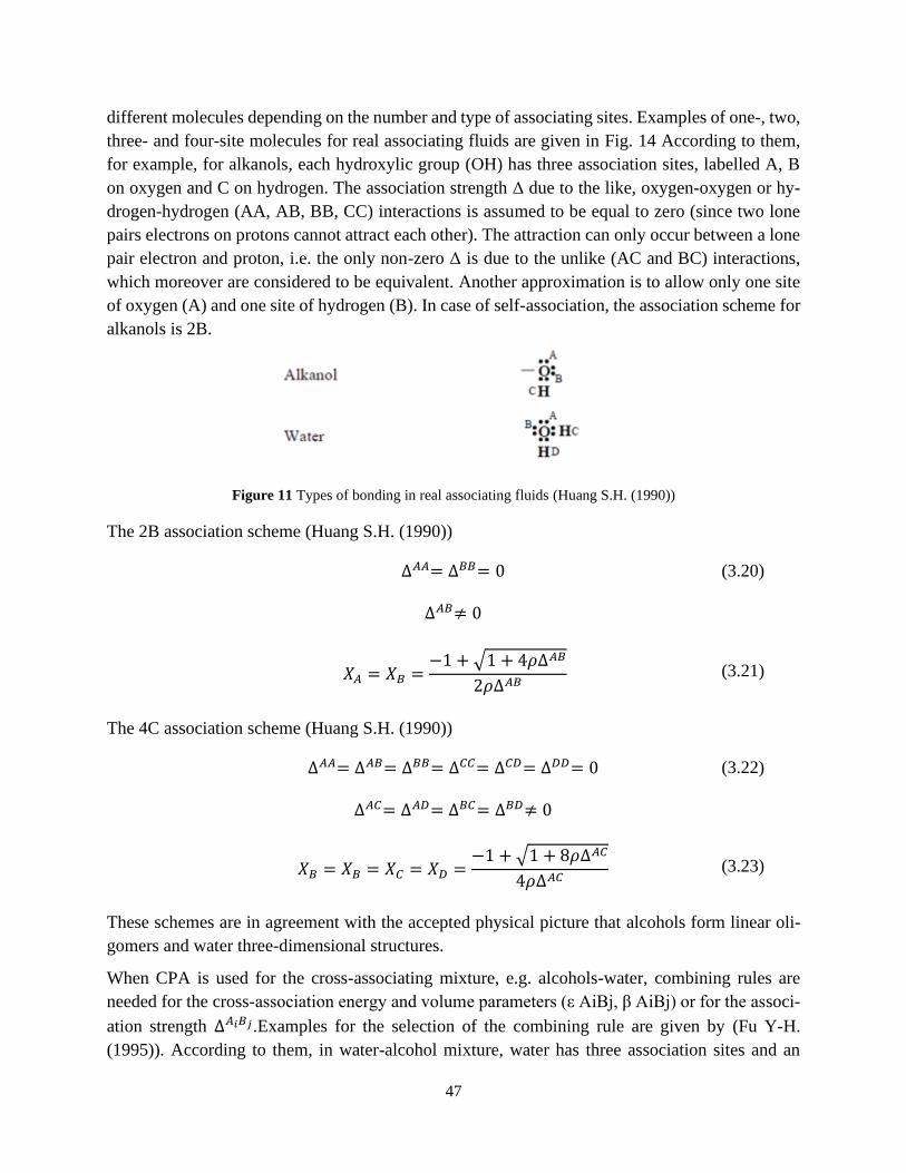
47

different molecules depending on the number and type of associating sites. Examples of one-, two,

three- and four-site molecules for real associating fluids are given in Fig. 14 According to them,

for example, for alkanols, each hydroxylic group (OH) has three association sites, labelled A, B

on oxygen and C on hydrogen. The association strength Δ due to the like, oxygen-oxygen or hy-

drogen-hydrogen (AA, AB, BB, CC) interactions is assumed to be equal to zero (since two lone

pairs electrons on protons cannot attract each other). The attraction can only occur between a lone

pair electron and proton, i.e. the only non-zero Δ is due to the unlike (AC and BC) interactions,

which moreover are considered to be equivalent. Another approximation is to allow only one site

of oxygen (A) and one site of hydrogen (B). In case of self-association, the association scheme for

alkanols is 2B.

Figure 11 Types of bonding in real associating fluids (Huang S.H. (1990))

The 2B association scheme (Huang S.H. (1990))

The 4C association scheme (Huang S.H. (1990))

These schemes are in agreement with the accepted physical picture that alcohols form linear oli-

gomers and water three-dimensional structures.

When CPA is used for the cross-associating mixture, e.g. alcohols-water, combining rules are

needed for the cross-association energy and volume parameters (ε AiBj, β AiBj) or for the associ-

ation strength ∆𝐴𝑖𝐵𝑗.Examples for the selection of the combining rule are given by (Fu Y-H.

(1995)). According to them, in water-alcohol mixture, water has three association sites and an

∆𝐴𝐴= ∆𝐵𝐵= 0 (3.20)

∆𝐴𝐵≠ 0

𝑋𝐴 = 𝑋𝐵 =

−1 + √1 + 4𝜌∆𝐴𝐵

2𝜌∆𝐴𝐵 (3.21)

∆𝐴𝐴= ∆𝐴𝐵= ∆𝐵𝐵= ∆𝐶𝐶= ∆𝐶𝐷= ∆𝐷𝐷= 0 (3.22)

∆𝐴𝐶= ∆𝐴𝐷= ∆𝐵𝐶= ∆𝐵𝐷≠ 0

𝑋𝐵 = 𝑋𝐵 = 𝑋𝐶 = 𝑋𝐷 =−1 + √1 + 8𝜌∆𝐴𝐶

4𝜌∆𝐴𝐶 (3.23)

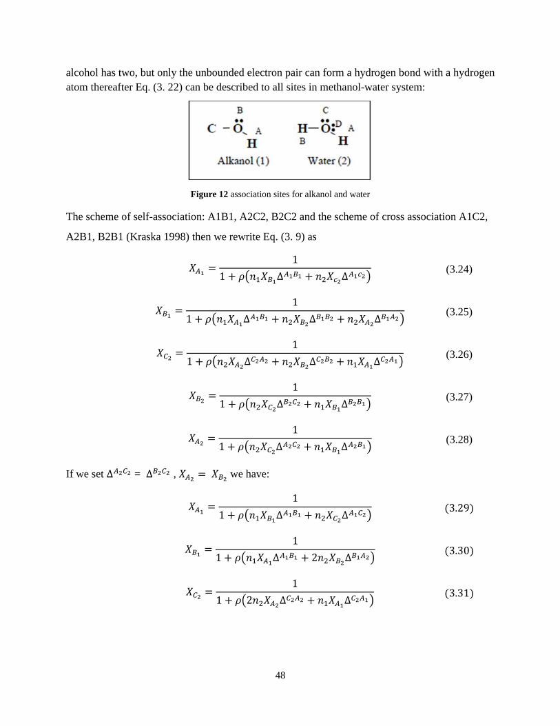
48

alcohol has two, but only the unbounded electron pair can form a hydrogen bond with a hydrogen

atom thereafter Eq. (3. 22) can be described to all sites in methanol-water system:

Figure 12 association sites for alkanol and water

The scheme of self-association: A1B1, A2C2, B2C2 and the scheme of cross association A1C2,

A2B1, B2B1 (Kraska 1998) then we rewrite Eq. (3. 9) as

If we set ∆𝐴2𝐶2 = ∆𝐵2𝐶2 , 𝑋𝐴2= 𝑋𝐵2

we have:

𝑋𝐴1=

1

1 + 𝜌(𝑛1𝑋𝐵1∆𝐴1𝐵1 + 𝑛2𝑋𝑐2

∆𝐴1𝑐2) (3.24)

𝑋𝐵1=

1

1 + 𝜌(𝑛1𝑋𝐴1∆𝐴1𝐵1 + 𝑛2𝑋𝐵2

∆𝐵1𝐵2 + 𝑛2𝑋𝐴2∆𝐵1𝐴2)

(3.25)

𝑋𝐶2=

1

1 + 𝜌(𝑛2𝑋𝐴2∆𝐶2𝐴2 + 𝑛2𝑋𝐵2

∆𝐶2𝐵2 + 𝑛1𝑋𝐴1∆𝐶2𝐴1)

(3.26)

𝑋𝐵2=

1

1 + 𝜌(𝑛2𝑋𝐶2∆𝐵2𝐶2 + 𝑛1𝑋𝐵1

∆𝐵2𝐵1) (3.27)

𝑋𝐴2=

1

1 + 𝜌(𝑛2𝑋𝐶2∆𝐴2𝐶2 + 𝑛1𝑋𝐵1

∆𝐴2𝐵1) (3.28)

𝑋𝐴1=

1

1 + 𝜌(𝑛1𝑋𝐵1∆𝐴1𝐵1 + 𝑛2𝑋𝐶2

∆𝐴1𝐶2) (3.29)

𝑋𝐵1=

1

1 + 𝜌(𝑛1𝑋𝐴1∆𝐴1𝐵1 + 2𝑛2𝑋𝐵2

∆𝐵1𝐴2) (3.30)

𝑋𝐶2=

1

1 + 𝜌(2𝑛2𝑋𝐴2∆𝐶2𝐴2 + 𝑛1𝑋𝐴1

∆𝐶2𝐴1) (3.31)

49

There are four non-linear equations with four variables and we can solve them simultaneously

using Newton-Raphson method with objective function (for all sites):

In order to simplify the problem further, all the cross-association energy and volume parameters

are taken to be equal and are estimated as follows:

According to (Derawi S.O. 2002) following mixing rules for the energy parameters shows good

Correlation with the experimental data on methanol-water system:

𝑋𝐴2= 𝑋𝐵2

=1

1 + 𝜌(𝑛2𝑋𝐶2∆𝐵2𝐶2 + 𝑛1𝑋𝐵1

∆𝐵2𝐵1) (3.32)

𝐹 ( ∑ 𝑋𝐴𝑖

𝑎𝑙𝑙 𝑠𝑖𝑡𝑒𝑠

𝑋𝐴𝑖

) = 𝑋𝐴1(1 + 𝜌 ∑𝑛𝑗

𝑗

∑𝑋𝐵𝑗

𝐵𝑖

) − 1 ≈ 0 (3.33)

휀𝐴1𝐵2 = 휀𝐵1𝐵2 = 휀𝐶1𝐴2 = √휀𝐴1𝑐1 휀𝐴2𝐵2 (3.34)

𝛽𝐴1𝐵2 = 𝛽𝐵1𝐵2 = 𝛽𝐶1𝐴2 =(𝛽𝐴1𝐶1 + 𝛽𝐴2𝐵2)

2 (3.35)

CR-1: 휀𝐴𝑖𝐵𝑗 =휀𝐴1𝐵1 + 휀𝐴2𝐵2

2 ; 𝛽𝐴𝑖𝐵𝑗 = √𝛽𝐴1𝐵1 + 𝛽𝐴2𝐵2 (3.36)

CR-2: 휀𝐴𝑖𝐵𝑗 = √휀𝐴1𝐵1 + 휀𝐴2𝐵2 ; 𝛽𝐴𝑖𝐵𝑗 = √𝛽𝐴1𝐵1 + 𝛽𝐴2𝐵2 (3.37)

Elliot Rule: ∆𝐴𝑖𝐵𝑗= √∆𝐴1𝐵1 + ∆𝐴2𝐵2 (3.38)

50

Chapter 4

4 Hydrates Thermodynamic Modelling

Predicting hydrate stability/formation conditions is crucial for oil and gas industry mainly to avoid

pipelines blockage during oil and gas transportation and supplying. Additionally, exploitation

methods of the natural gas in hydrate started gaining attention in the last years for which under-

standing under what conditions hydrates are stable or can be stabilized is also important. Based on

that, in this Chapter we will begin with a quick review of relatively simple hand calculations, while

the main objective is to discuss original and modified van der Waals-Platteeuw (vdW-P) theory

and finishing with implementation of this theory in different computer-based calculations using

different rigorous thermodynamic models present in different software used in this study.

4.1 Introduction and Review of First Hydrate Prediction Methods

Hydrate hand prediction methods for hydrate stability were largely developed between 1940s and

1950s and based mainly on experimental work. These relatively simple and eloquent methods,

before the days of computers, were powerful in allowing one to predict hydrate stability for the

first time, often quite accurately (Wilcox WI 1941). However, sH hydrate structure had not yet

been discovered at this time, these early hand calculation models can be applied only to the sI and

sII hydrates. Most popular and widely used hand calculations methods are the gas gravity and the

k-value methods. The “Gas Gravity Method” is the simplest method for predicting hydrate for-

mation at three-phase hydrate-liquid water-vapor equilibrium. This method was presented by Katz

in 1945 and it is based solely on one data information the density of a natural gas. Plotted on a P-

T diagram. As the work of Katz mainly considered hydrates formed from natural gasses, the gas

gravity method should be used only for systems of natural gasses with low contents of non-com-

bustible compounds (such as e.g. carbon dioxide, nitrogen etc.) (Sloan ED 2008). Another method

was developed a few years earlier, called the “distribution coefficient method” or in short, the “K-

value method”. The K-value method assumes ideal solution of gas phase constituents in the solid

hydrate phase. Under this assumption, a distribution coefficient of each hydrate former is defined

as

Where 𝑦𝑖 is the vapor phase mole fraction of component i and 𝑌𝑖 is the water-free hydrate mole

fraction of component 𝑖.Water-free means that the mole fraction is calculated only on basis of the

hydrate phase guest contents. Again, charts were produced, presenting K-values as function of

temperature and pressure for individual hydrate formers.

𝐾𝑣−𝑠,𝑖 =𝑦𝑖

𝑌𝑖 (4.1)

51

Using of these charts and the following constraint

Hydrate formation conditions could be estimated by an iterative solution approach.

K-value method provides accurate temperature/pressure dissociation conditions for light gases

found in typical natural gases. On the other hand, this method shown deviation from experimental

data for

• Mixtures with high ethane, propane and butane contents.

• Two gases of main interest in this work, carbon dioxide and nitrogen (Sloan ED 2008).

4.2 Original Van Der Waals-Platteeuw Hydrate Model

The van der Waals-Platteeuw hydrate theory was proposed by J. H. van der Waals and J. C. Plat-

teeuw in 1958 (J.H.van der Waals 1959). vdW-P treats the solid phase only and is combined with

an equation of state and an activity coefficient model for the description of co-existing fluid phases.

Nowadays the typical equation of state used in this model is CPA EoS explained in chapter 3 since

it covers all type of fluids. The basic theory behind the model presented by van der Waals and

Platteeuw is often claimed to come from statistical mechanics. (Sloan ED 2008) Have shown a

detailed derivation of the model equations by the use of statistical mechanics. However, the model

can similarly be derived by use of chemical reaction theory and classical thermodynamic relations.

The main assumption in the Van der Waals-Platteeuw theory is the chemical potential of water in

the hydrate phase. As it has been shown in Chapter 2 that at equilibrium, the chemical potential

must be equal in all phases present at. As an example of hydrate case and in the locus of hydrate

(H) – Ice (I) – vapor (V) equilibrium, the following expression must be satisfied:

The idea of vdW-P followed the same Three-Step procedure mentioned in Chapter 2 where they

spliced the problem into three Steps. In Step 1 they assumed that water will form empty cage with

the same structure conditions (e.g. same volume) as actual hydrates but without the presence of

guest molecule inside. Step 2 evaluate the chemical potential of water in this theoretical empty

hydrate and after that imply the physics in step 3 so that the problem will be physically valuable.

Step 3 implies the adsorption of gas guest molecules into the empty hydrate cage. By doing that

they solved the hydrate problem indirectly but implementing the main engineering paths so to have

a solution of the real difficult problem. This meta-stable hydrate crystalline water β-phase that

constituted the same structure of water as in the actual hydrate, cannot be present or formed ex-

perimentally. This is present due to the fact that hydrate is formed and stabilized given that pressure

inside of crystalline hydrate cages is equal to pressure outside so no burst or collapse of hydrate

cages may happen. This stabilization is present by the interaction between the guest molecule (gas)

∑𝑦𝑖

𝐾𝑣−𝑠,𝑖

𝑛

𝑖=1

(4.2)

𝜇𝑤𝑎𝑡𝑒𝑟 𝐻𝑦𝑑𝑟𝑎𝑡𝑒

= 𝜇𝑤𝑎𝑡𝑒𝑟 𝐼𝑐𝑒 = 𝜇𝑤𝑎𝑡𝑒𝑟

𝑉𝑎𝑝𝑜𝑟 (4.3)

52

and its surrounding water molecules forming the cage. In the following sections of this chapter we

will describe vdW-P theory for the second locus of P-T diagram hydrate forming (Hydrate (H) –

Liquid water (Lw) – vapor (V)).

The difference in chemical potential of actual hydrate phase and meta-stable β-phase can be de-

scribed as following:

For Step 3 in which the adsorption of guest molecules in empty cavities has been taken into con-

sideration an adsorption theory is required. This step can be described by an approach similar to

Langmuir adsorption theory using Lennard-Jones-Devonshire theory for the description of the

Langmuir adsorption coefficients. (Prausnitz W. 1972).

In order to do so, several assumptions have to be taken into consideration (Prausnitz W. 1972)

such as:

1) All cavities are assumed spherical.

2) Each cavity can contain one guest at most.

3) Guest-Guest interactions are negligible.

4) The guest molecule does not distort the structural properties of the water lattice.

5) The internal partition function of the guest is considered to be identical to that of the gas in its

ideal state.

6) Only London forces are considered in the guest-host interaction.

The main reason for these assumptions goes back to monolayer adsorption theory of Langmuir

that will be used while additional assumptions will be discussed later in the appropriate sections.

As it is mentioned before that the difference in chemical potential of water between the theoretical

empty hydrate water lattice (empty cavities) and the actual hydrate is the presence of guest mole-

cules in the water cavities, according to monolayer Langmuir adsorption theory this difference can

illustrated in Fig.13 and described as following:

where

• 𝑣𝑚 is the number of cavities type m per water molecule in the hydrate structure.

• 𝜃(𝑇, 𝑃, �̅�)𝑚.𝑗 is the fractional occupancy of component j in cavity type m

• 𝑅 is the universal, or ideal gas constant.

∆𝜇𝑤𝛽−𝐻

= 𝜇𝑤𝛽

− 𝜇𝑤𝐻 (4.4)

∆𝜇(𝑇, 𝑃, 𝜃)𝑤𝛽−𝐻

= −𝑅. 𝑇.∑[𝑣𝑚 . ln (1 − ∑𝜃(𝑇, 𝑃, �̅�)𝑚.𝑗

𝑗

)]

𝑚

(4.5)

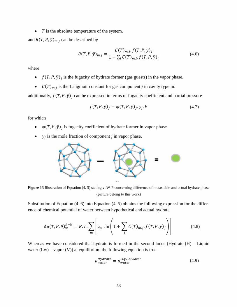
53

• 𝑇 is the absolute temperature of the system.

and 𝜃(𝑇, 𝑃, �̅�)𝑚.𝑗 can be described by

where

• 𝑓(𝑇, 𝑃, �̅�)𝑗 is the fugacity of hydrate former (gas guests) in the vapor phase.

• 𝐶(𝑇)𝑚,𝑗 is the Langmuir constant for gas component j in cavity type m.

additionally, 𝑓(𝑇, 𝑃, �̅�)𝑗 can be expressed in terms of fugacity coefficient and partial pressure

for which

• 𝜑(𝑇, 𝑃, �̅�)𝑗 is fugacity coefficient of hydrate former in vapor phase.

• 𝑦𝑗 is the mole fraction of component j in vapor phase.

Figure 13 Illustration of Equation (4. 5) stating vdW-P concerning difference of metastable and actual hydrate phase

(picture belong to this work)

Substitution of Equation (4. 6) into Equation (4. 5) obtains the following expression for the differ-

ence of chemical potential of water between hypothetical and actual hydrate

Whereas we have considered that hydrate is formed in the second locus (Hydrate (H) – Liquid

water (Lw) – vapor (V)) at equilibrium the following equation is true

𝜃(𝑇, 𝑃, �̅�)𝑚.𝑗 =𝐶(𝑇)𝑚,𝑗. 𝑓(𝑇, 𝑃, �̅�)𝑗

1 + ∑ 𝐶(𝑇)𝑚,𝑙.𝑙 𝑓(𝑇, 𝑃, �̅�)𝑙 (4.6)

𝑓(𝑇, 𝑃, �̅�)𝑗 = 𝜑(𝑇, 𝑃, �̅�)𝑗. 𝑦𝑗 . 𝑃 (4.7)

∆𝜇(𝑇, 𝑃, 𝜃)𝑤𝛽−𝐻

= 𝑅. 𝑇.∑[𝑣𝑚 . ln (1 + ∑ 𝐶(𝑇)𝑚,𝑗. 𝑓(𝑇, 𝑃, �̅�)𝑗

𝑗

)]

𝑚

(4.8)

𝜇𝑤𝑎𝑡𝑒𝑟 𝐻𝑦𝑑𝑟𝑎𝑡𝑒

= 𝜇𝑤𝑎𝑡𝑒𝑟 𝐿𝑖𝑞𝑢𝑖𝑑 𝑤𝑎𝑡𝑒𝑟

(4.9)

54

in which chemical potential of water is as following

where

• 𝜇(𝑇, 𝑃)𝑤𝑝

is the chemical potential of pure liquid water

• γ is the activity coefficient of water in the non- ideal liquid phase at the presence of hydrogen

bonding or electrolyte components in the liquid phase (e.g. MEG, Salts).

However, several studies have shown that solubility of hydrocarbons gasses is very low in which

the activity coefficient can be assumed unity (close to ideal). However, in case of carbon dioxide

and nitrogen the solubility is countable where the activity coefficient is calculated properly. On

the other hand, activity coefficient is important in hydrate case in the presence of salts and alcohols.

Activity coefficient can be modeled either with symmetric activity coefficient model 𝛾 or in terms

of fugacity coefficients 𝜑 as following

where 𝑥𝑤𝐿𝑤 is the liquid phase composition in water.

Defining the difference of chemical potential between the theoretical clathrate and a pure water

liquid phase thusly

Substituting Eq. (4. 4), (4. 9), (4. 10), (4. 11) and (4. 12) hence ∆𝜇(𝑇, 𝑃)𝑤𝛽−𝐿𝑤 can be formulated

as

or

𝜇𝑤𝑎𝑡𝑒𝑟 𝐿𝑖𝑞𝑢𝑖𝑑 𝑤𝑎𝑡𝑒𝑟 = 𝜇(𝑇, 𝑃)𝑤

𝑝 + 𝑅. 𝑇. 𝑙𝑛[𝛾(𝑇, 𝑃, �̅�)𝑤𝐿𝑤] (4.10)

𝛾(𝑇, 𝑃, �̅�)𝑤𝐿𝑤 = 𝑥𝑤

𝐿𝑤 . 𝛾(𝑇, 𝑃, �̅�)𝑤𝐿𝑤 = 𝑥𝑤

𝐿𝑤 .𝜑(𝑇, 𝑃, �̅�)𝑤

𝐿𝑤

𝜑(𝑇, 𝑃)𝑤𝑝 (4.11)

∆𝜇(𝑇, 𝑃)𝑤𝛽−𝐿𝑤 = 𝜇(𝑇, 𝑃)𝑤

𝛽− 𝜇(𝑇, 𝑃)𝑤

𝑃 𝐿𝑤 (4.12)

∆𝜇(𝑇, 𝑃)𝑤𝛽−𝐿𝑤 = 𝑅. 𝑇.∑[𝑣𝑚 . ln (1 + ∑𝐶(𝑇)𝑚,𝑗. 𝑓(𝑇, 𝑃, �̅�)𝑗

𝑗

)]

𝑚

+ 𝑅. 𝑇. ln [𝑥𝑤𝐿𝑤 .

𝜑(𝑇, 𝑃, �̅�)𝑤𝐿𝑤

𝜑(𝑇, 𝑃)𝑤𝑝 ]

(4.13)

∆𝜇(𝑇, 𝑃)𝑤

𝛽−𝐿𝑤 = 𝑅. 𝑇.∑[𝑣𝑚 . 𝑙𝑛 (1 + ∑𝐶(𝑇)𝑚,𝑗 . 𝑓(𝑇, 𝑃, �̅�)𝑗

𝑗

)]

𝑚

+ 𝑅. 𝑇. 𝑙𝑛[𝑥𝑤𝐿𝑤 . 𝛾(𝑇, 𝑃, �̅�)𝑤

𝐿𝑤]

(4.14)

55

Keep in mind that all fugacity and fugacity coefficients in Eq. (4. 14) can be calculated using CPA

EoS explained in Chapter 3. Alternatively, some approaches tested in this work use activity coef-

ficient model where Eq. (4. 14) is used.

4.2.1 Langmuir Adsorption Coefficient 𝑪(𝑻)𝒎,𝒋

(J.H.van der Waals 1959) Suggested that the Langmuir adsorption coefficients may be approxi-

mated using Lennard-Jones-Devonshire cell theory for example Lennard-Jones 12-6 cell potential.

They suggested the usage of the following expression

for which

• 𝑘𝐵 is Boltzmann constant.

• 𝑤(𝑟)𝑚.𝑗 is the spherical core cell potential of component j in cavity type m.

• 𝑟 is the linear distance from the center of the cell.

Several researchers investigated different cell potentials for use in hydrate dissociation pressure

calculations. The most suitable for this kind of calculation is Kihara cell potential (McKoy 1963).

They work where based on evaluating the interactions between the guest molecule and all its sur-

rounding first layer of water molecules forming cages and summed up the contributions in one

expression for the spherical core cell potential. In the years after, (Prausnitz W. 1972) were the

first who presented an algorithm for vdW-P for hydrate model for computer calculation and

slightly modified the expression provided by (McKoy 1963) to became:

where

• 𝑧𝑚 is the coordination number for the guest in cavity type 𝑚.

• 휀𝑗 is the characteristic energy of guest molecule 𝑗.

• 𝑎𝑗 is the core radius of molecule 𝑗.

• 𝜎𝑗+2𝑎𝑗 is the collision diameter of molecule 𝑗.

• 𝑅𝑚 is the radius of cavity type m.

And 𝛿(𝑁)𝑚,𝑗 is reported as

𝐶(𝑇)𝑚,𝑗 =4 ∙ 𝜋

(𝑘𝐵. 𝑇).∫ 𝑒𝑥𝑝 [

−𝑤(𝑟)𝑚.𝑗

(𝑘𝐵. 𝑇)]

∞

0

. 𝑟2. 𝑑𝑟 (4.15)

𝑤(𝑟)𝑚.𝑗 = 2. 𝑧𝑚. 휀𝑗 .

[

𝜎𝑗12

𝑅𝑚11. 𝑟

. (𝛿(𝑁 = 10)𝑚,𝑗 +𝑎𝑗

𝑅𝑚. 𝛿(𝑁 = 11)𝑚,𝑗)

−𝜎𝑗

6

𝑅𝑚5 . 𝑟

. (𝛿(𝑁 = 4)𝑚,𝑗 +𝑎𝑗

𝑅𝑚. 𝛿(𝑁 = 5)𝑚,𝑗)

]

(4.15)

56

Different methods have been investigated to solve the integral of Langmuir constant in Eq. (4. 15)

such as Simpson 3/8 rule and the Gauss-Legendre Quadrature method.

4.3 Parrish and Prausnitz Hydrate Modelling

Parrish and Prausnitz (Prausnitz W. 1972) hydrate modeling carried out in CSMHyd Software

(Colorado School of Mineral)

4.3.1 Model Theory

(Prausnitz W. 1972) Have implemented vdW-P theory of hydrate to be in a state suitable for com-

puter calculation. P-P presented hydrate-gas equilibria calculation for multicomponent gas systems

based on the usage of Kihara (spherical-core). The ideas of these researches are as following.

With theoretical chemical potential derived by (J.H.van der Waals 1959) showed in the last section,

(Prausnitz W. 1972) proposed a method for calculating the chemical potential difference by the

use of experimental reference hydrate. This method took advantage on the fact that chemical po-

tential is a state function and by integrating the value of experimental reference hydrate, chemical

potential of hydrate at desired pressure and temperature can be calculated. They defined a reference

hydrate at reference temperature, To, and reference pressure, Po, where the integration to the de-

sired state is done following two steps. First step aims to transform the measured chemical poten-

tial difference from reference temperature To, to the actual temperature T and from reference Po at

reference temperature To, to the reference pressure PR at the actual temperature, T.In the second

step, the chemical potential difference is transformed from the reference pressure PR to the actual

pressure P. two steps are as following:

Step 1:

where

• ∆𝜇(𝑇, 𝑃𝑅)𝑤𝛽−𝐿𝑤 is the chemical potential difference between theoretical empty hydrate and liq-

uid water at temperature 𝑇 and at the dissociation pressure of the reference pressure𝑃𝑅.

• ∆𝜇(𝑇0, 𝑃0)𝑤𝛽−𝐿𝑤 is the chemical potential difference between theoretical empty hydrate and

liquid water at temperature 𝑇0 and at the dissociation pressure of the reference pressure P0.

𝛿(𝑁)𝑚,𝑗 =1

𝑁. [(1 − 𝑟. 𝑅𝑚

−1 − 𝑎𝑗 . 𝑅𝑚−1)

−𝑁− (1 + 𝑟. 𝑅𝑚

−1 − 𝑎𝑗 . 𝑅𝑚−1)

−𝑁] (4.17)

∆𝜇(𝑇, 𝑃𝑅)𝑤𝛽−𝐿𝑤

𝑅. 𝑇

=∆𝜇(𝑇0, 𝑃0)𝑤

𝛽−𝐿𝑤

𝑅. 𝑇0− ∫

∆𝐻(𝑇0, 𝑃0)𝑤𝛽 𝐼𝑐𝑒⁄

+ ∆𝐻(𝑇)𝑤𝐼𝑐𝑒 𝐿𝑤⁄

𝑅. 𝑇2

𝑇

𝑇0

𝑑𝑇

+ ∫∆𝑉𝑤

𝛽 𝐼𝑐𝑒⁄+ ∆𝑉(𝑇)𝑤

𝐼𝑐𝑒 𝐿𝑤⁄

𝑅. 𝑇

𝑇

𝑇0

.𝑑𝑃𝑅

𝑑𝑇𝑑𝑇

(4.18)

57

• ∆𝐻(𝑇0, 𝑃0)𝑤𝛽 𝐼𝑐𝑒⁄

is the molar enthalpy difference between empty hydrate and ice.

• ∆𝐻(𝑇)𝑤𝐼𝑐𝑒 𝐿𝑤⁄

is the molar enthalpy difference between ice and liquid water.

• ∆𝑉𝑤𝛽 𝐼𝑐𝑒⁄

is the difference in molar volume of the empty hydrate and ice measured for the ref-

erence hydrate.

• ∆𝑉(𝑇)𝑤𝐼𝑐𝑒 𝐿𝑤⁄

is the difference in molar volume of ice and liquid water.

• 𝑑𝑃𝑅

𝑑𝑇 is the slope of the measured dissociation pressure-temperature curve reported by

(Prausnitz W. 1972) for the reference hydrate.

Parrish and Prausnitz didn’t reported how they obtained this function. In addition, no place this

derivative is present. However, in this work we have derived this function for better understanding

and explanations of results.

For pure species ∆𝜇𝑤 = ∆𝐺𝑤 (4. 20) and ∆Gw = 𝑉∆𝑃 − 𝑆∆𝑇 (4. 21) where

Splicing each parameter into phase intervals (Ice – Liquid water)

Rearranging and integrating Eq. (4. 24)

∆𝜇𝑤𝛽−𝐿𝑤

𝑅𝑇=

𝜇𝑤𝛽

− 𝜇𝑤𝐿𝑤

𝑅𝑇=

𝜇𝑤𝛽

𝑅𝑇−

𝜇𝑤𝐿

𝑅𝑇 =

𝜇𝑤0

𝛽

𝑅𝑇0−

𝜇𝑤0𝐿

𝑅𝑇0+

𝜇𝑤𝛽

𝑅𝑇−

𝜇𝑤𝐿

𝑅𝑇

=∆𝜇𝑤0

𝑅𝑇0+

∆𝜇𝑤𝛽−𝐿𝑤

𝑅𝑇

(4.19)

S = ∆H

𝑇 (4.22)

∆𝜇𝑤

𝛽−𝐿𝑤

𝑅𝑇=

∆𝜇𝑤0

𝛽−𝐿𝑤

𝑅𝑇0+

𝑉𝛽−𝐿𝑤𝑑𝑃

𝑅𝑇−

(∆𝐻)𝛽−𝐿𝑤𝑑𝑇

𝑅𝑇2 (4.23)

∆𝜇𝑤𝛽−𝐿𝑤

𝑅𝑇 =

∆𝜇𝑤0

𝛽−𝐿𝑤

𝑅𝑇0+ [

𝑉𝛽−𝐼𝑐𝑒

𝑅𝑇𝑑𝑃 +

𝑉𝐼𝑐𝑒 𝐿𝑤⁄

𝑅𝑇𝑑𝑃]

− [∆𝐻𝛽−𝐼𝑐𝑒

𝑅𝑇2𝑑𝑇 +

∆𝐻𝐼𝑐𝑒 𝐿𝑤⁄

𝑅𝑇2𝑑𝑇]

(4.24)

∆𝜇𝑤𝛽−𝐿𝑤

𝑅𝑇=

∆𝜇𝑤0

𝛽−𝐿𝑤

𝑅𝑇0

+ [∫𝑉𝛽−𝐼𝑐𝑒 + 𝑉𝐼𝑐𝑒 𝐿𝑤⁄

𝑅𝑇𝑑𝑃 − ∫

∆𝐻𝛽−𝐼𝑐𝑒 + ∆𝐻𝐼𝑐𝑒 𝐿𝑤⁄

𝑅𝑇2𝑑𝑇

𝑇

𝑇0

𝑃

𝑃0

]

(4.25)

58

Replacing 𝑑𝑃 by slope of pressure-temperature reference diagram provided by Parrish and

Prausnitz 𝑑𝑃𝑅

𝑑𝑇 in Eq. (4. 25) so to have the general form present in Eq. (4. 18)

It should be noted that ∆𝐻(𝑇)𝑤𝐼𝑐𝑒 𝐿𝑤⁄

is function of two terms, the first one is the change of enthalpy

due to the phase change from ice to liquid at the reference temperature and the second term is the

heat capacity of liquid water contribution of the heating from the reference temperature to the

actual temperature. These two terms are covered in the following equation:

Parrish and Prausnitz presented the reference pressure 𝑃0 as the vapor pressure of ice at tempera-

ture 𝑇0 and since this pressure is too small with respect to hydrate dissociation pressure it is as-

sumed 0.

Step 2:

where

• ∆𝜇(𝑇, 𝑃)𝑤𝛽−𝐿𝑤 Is the actual chemical potential difference between theoretical empty hy-

drate and liquid water at temperature 𝑇 and at the dissociation pressure of the actual pres-

sure 𝑃.

• ∆𝜇(𝑇, 𝑃𝑅)𝑤𝛽−𝐿𝑤 Is the chemical potential difference between theoretical empty hydrate and

liquid water at temperature 𝑇 and at the dissociation pressure of the reference pressure 𝑃𝑅

calculated in Step 1.

Parrish and Prausnitz (Prausnitz W. 1972) provided a three parameters expression for the temper-

ature dependence of the reference hydrate dissociation pressure:

And as it is obvious that dissociation pressure is gas composition dependence that may form struc-

ture sI and sII, (Prausnitz W. 1972) used as a reference hydrate for sI for temperature below 0°C

xenon and methane hydrate for temperature above this temperature. For sII bromochlorodifluoro-

methane hydrate has been considered as reference hydrate for temperature below 0°C and natural

gas mixture hydrate data above it. The values are shown in the following Table 1.

∆𝐻(𝑇)𝑤𝐼𝑐𝑒 𝐿𝑤⁄

= ∆𝐻(𝑇0, 𝑃0)𝑤𝐼𝑐𝑒 𝐿𝑤⁄

+ ∆𝐶𝑝(𝑇). (𝑇 − 𝑇0) (4.26)

∆𝜇(𝑇, 𝑃)𝑤

𝛽−𝐿𝑤 = ∆𝜇(𝑇, 𝑃𝑅)𝑤𝛽−𝐿𝑤

+ (∆𝑉𝑤𝛽 𝐼𝑐𝑒⁄

+ ∆𝑉(𝑇)𝑤𝐼𝑐𝑒 𝐿𝑤⁄

) . (𝑃 − 𝑃𝑅) (4.27)

ln[𝑃𝑅 𝑎𝑡𝑚⁄ ] = 𝐴𝑅 +𝐵𝑅

𝑇+ 𝐶𝑅 . ln 𝑇 (4.28)

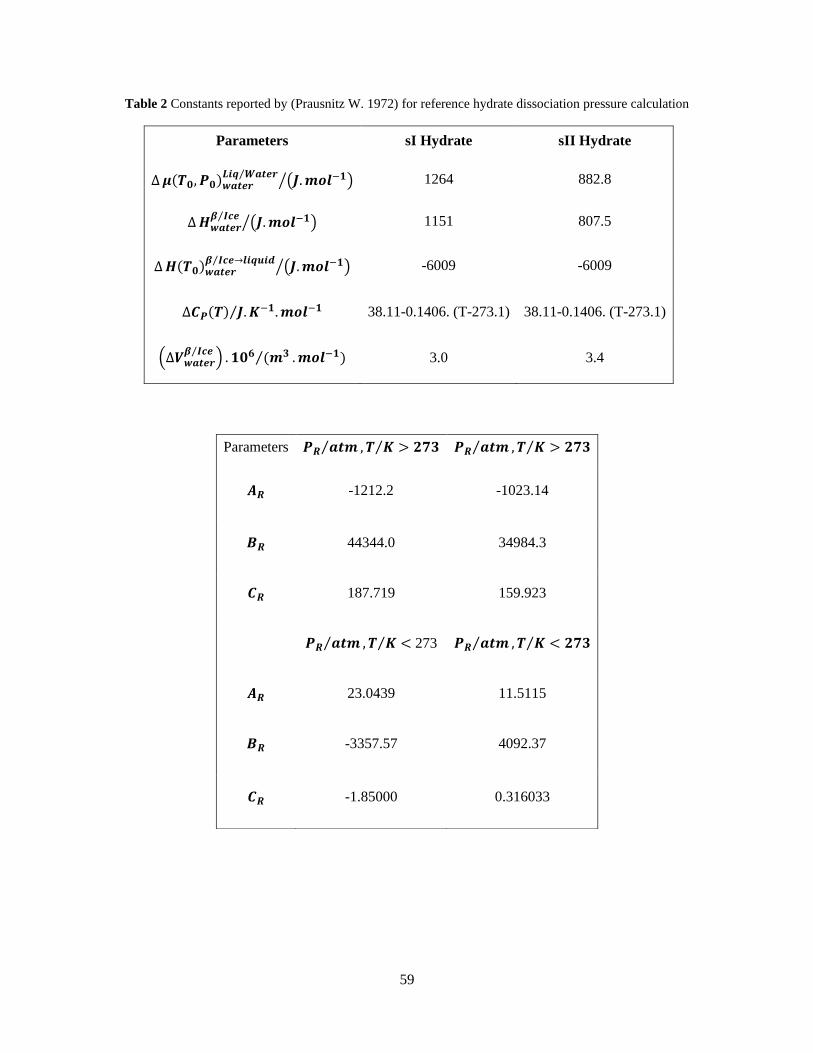
59

Table 2 Constants reported by (Prausnitz W. 1972) for reference hydrate dissociation pressure calculation

Parameters 𝑷𝑹 𝒂𝒕𝒎⁄ , 𝑻 𝑲⁄ > 𝟐𝟕𝟑 𝑷𝑹 𝒂𝒕𝒎⁄ , 𝑻 𝑲⁄ > 𝟐𝟕𝟑

𝑨𝑹 -1212.2 -1023.14

𝑩𝑹 44344.0 34984.3

𝑪𝑹 187.719 159.923

𝑷𝑹 𝒂𝒕𝒎⁄ , 𝑻 𝑲⁄ < 273 𝑷𝑹 𝒂𝒕𝒎⁄ , 𝑻 𝑲⁄ < 𝟐𝟕𝟑

𝑨𝑹 23.0439 11.5115

𝑩𝑹 -3357.57 4092.37

𝑪𝑹 -1.85000 0.316033

Parameters sI Hydrate sII Hydrate

∆𝝁(𝑻𝟎, 𝑷𝟎)𝒘𝒂𝒕𝒆𝒓𝑳𝒊𝒒 𝑾𝒂𝒕𝒆𝒓⁄

(𝑱.𝒎𝒐𝒍−𝟏)⁄ 1264 882.8

∆𝑯𝒘𝒂𝒕𝒆𝒓𝜷 𝑰𝒄𝒆⁄

(𝑱.𝒎𝒐𝒍−𝟏)⁄ 1151 807.5

∆𝑯(𝑻𝟎)𝒘𝒂𝒕𝒆𝒓𝜷 𝑰𝒄𝒆→𝒍𝒊𝒒𝒖𝒊𝒅⁄

(𝑱.𝒎𝒐𝒍−𝟏)⁄ -6009 -6009

∆𝑪𝑷(𝑻) 𝑱.𝑲−𝟏.𝒎𝒐𝒍−𝟏⁄ 38.11-0.1406. (T-273.1) 38.11-0.1406. (T-273.1)

(∆𝑽𝒘𝒂𝒕𝒆𝒓𝜷 𝑰𝒄𝒆⁄

) . 𝟏𝟎𝟔 (𝒎𝟑⁄ .𝒎𝒐𝒍−𝟏) 3.0 3.4

60

In addition, P-P proposed an expression for calculation of the Langmuir adsorption coefficients

and noted that this expression is favorable in the temperature range (260-300) K. they recom-

mended the usage of this expression for simplicity in the temperature range while for temperature

outside of it, Kihara cell potential (Eq. 4. 16) should be used with parameters of Table 2. However,

they stated that the proposed equation for Langmuir adsorption coefficients deviation is 0.2% or

less for each gas in the temperature range. The proposed expression given as

where

• 𝐴𝑚𝑗 And 𝐵𝑚𝑗 are fitting parameters related to guest type 𝑗 in cavity type m present in Table 3.

In case of occupancy of a guest in both structure sI for example methane where sI hydrate structure

include two cavity type four fitting parameter is required for this guest.

Table 3 Kihara Parameters reported by (Prausnitz W. 1972) used in CSMHyd

𝐶𝑚𝑗(𝑇) = (𝐴𝑚𝑗

𝑇) 𝑒𝑥𝑝 (

𝐵𝑚𝑗

𝑇) (4.29)

Gas 𝟐𝒂𝒋, Å 𝝈,Å 𝝐/𝒌 °K

Methane 0.600 3.2398 153.17

Ethane 0.800 3.3180 174.97

Ethylene 0.940 3.2910 172.87

Propane 1.360 3.3030 200.94

Propylene 1.300 3.2304 202.42

Cyclopropane 1.000 3.4559 210.58

Isobutene 1.600 3.1244 220.52

Nitrogen 0.700 3.6142 127.95

Oxygen 0.720 2.7673 166.37

Carbone dioxide 0.720 2.9681 169.09

Hydrogen sulfide 0.720 3.1558 205.84

Argon 0.368 2.9434 170.50

Krypton 0.460 2.9739 198.34

Xenon 0.560 3.1906 201.34

Sulfur hexafluoride 1.620 3.1379 220.73

61

During describing hydrate modeling three step procedure that Van-der-Waals -Platteeuw have

used to describe and solve the problem, many assumptions has been made regarding the solution

of Step 3 (adsorption phenomenon). However, one major assumption is that guest molecule does

not distort the structural properties of the water lattice. This assumption means that the Gibbs

energy change is only due to adsorption of guest molecule with no volume change of the cages

when gas is adsorbed in. Parrish and Prausnitz took advantage of this assumption and equalized

the theoretical chemical potential difference of each state to its equivalent experimental one so to

be able to solve the problem directly for dissociation pressure or temperature.

Note that all equations derived above can be implied only for second locus of P-T hydrate equilib-

rium (above ice-point). For equilibrium calculation below ice point (first locus) Eq. (4. 14) will be

and Eq. (4. 18)

and new parameter is required for Eq. (4. 19) while Eq. (4. 20) will be

Now in CSMHyd Software Parish and Prausnitz has been implemented with a modification of

Two-step calculation which has been replaced by (Holder 1988) equation. This equation elimi-

nated the need for the reference pressure and thus simplified the calculations given us:

∆𝜇(𝑇, 𝑃)𝑤𝛽−𝐼𝑐𝑒𝑤 = 𝑅. 𝑇.∑[𝑣𝑚 . 𝑙𝑛 (1 + ∑𝐶(𝑇)𝑚,𝑗 . 𝑓(𝑇, 𝑃, �̅�)𝑗

𝑗

)]

𝑚

(4.29)

∆𝜇(𝑇, 𝑃𝑅)𝑤𝛽−𝐼𝑐𝑒𝑤

𝑅. 𝑇

=∆𝜇(𝑇0, 𝑃0)𝑤

𝛽−𝐼𝑐𝑒𝑤

𝑅. 𝑇0− ∫

∆𝐻(𝑇0, 𝑃0)𝑤𝛽 𝐼𝑐𝑒⁄

𝑅. 𝑇2

𝑇

𝑇0

𝑑𝑇

+ ∫∆𝑉𝑤

𝛽 𝐼𝑐𝑒⁄

𝑅. 𝑇

𝑇

𝑇0

.𝑑𝑃𝑅

𝑑𝑇𝑑𝑇

(4.30)

∆𝜇(𝑇, 𝑃)𝑤𝛽−𝐼𝑐𝑒𝑤 = ∆𝜇(𝑇, 𝑃𝑅)𝑤

𝛽−𝐼𝑐𝑒𝑤 + (∆𝑉𝑤𝛽 𝐼𝑐𝑒⁄

) . (𝑃 − 𝑃𝑅) (4.31)

∆𝜇(𝑇, 𝑃)𝑤𝐿𝑤

𝑅. 𝑇=

∆𝜇(𝑇0, 𝑃0)𝑤𝐿𝑤

𝑅. 𝑇0− ∫

∆𝐻(𝑇0, 𝑃0)𝑤𝛽 𝐼𝑐𝑒⁄

+ ∆𝐻(𝑇)𝑤𝐼𝑐𝑒 𝐿𝑤⁄

𝑅. 𝑇2

𝑇

𝑇0

𝑑𝑇

+ ∫∆𝑉𝑤

𝛽 𝐼𝑐𝑒⁄+ ∆𝑉(𝑇)𝑤

𝐼𝑐𝑒 𝐿𝑤⁄

𝑅. 𝑇

𝑃

0

. 𝑑𝑃

(4.32)

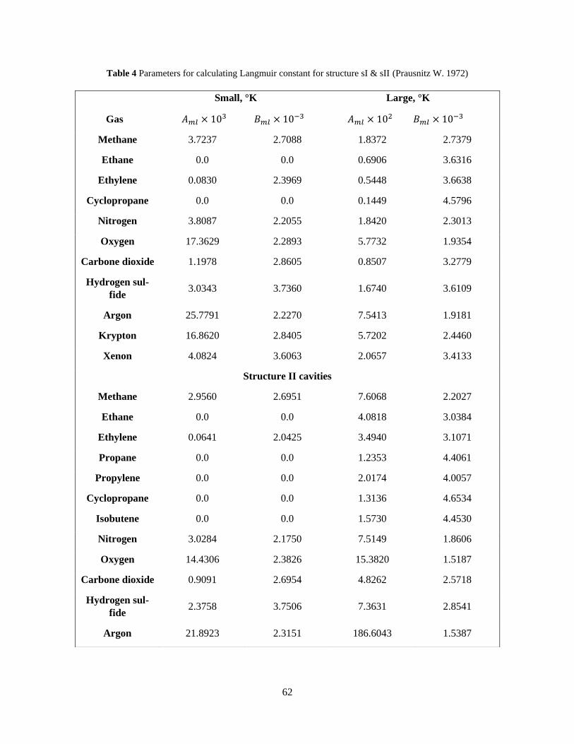
62

Table 4 Parameters for calculating Langmuir constant for structure sI & sII (Prausnitz W. 1972)

Small, °K Large, °K

Gas 𝐴𝑚𝑙 × 103 𝐵𝑚𝑙 × 10−3 𝐴𝑚𝑙 × 102 𝐵𝑚𝑙 × 10−3

Methane 3.7237 2.7088 1.8372 2.7379

Ethane 0.0 0.0 0.6906 3.6316

Ethylene 0.0830 2.3969 0.5448 3.6638

Cyclopropane 0.0 0.0 0.1449 4.5796

Nitrogen 3.8087 2.2055 1.8420 2.3013

Oxygen 17.3629 2.2893 5.7732 1.9354

Carbone dioxide 1.1978 2.8605 0.8507 3.2779

Hydrogen sul-

fide 3.0343 3.7360 1.6740 3.6109

Argon 25.7791 2.2270 7.5413 1.9181

Krypton 16.8620 2.8405 5.7202 2.4460

Xenon 4.0824 3.6063 2.0657 3.4133

Structure II cavities

Methane 2.9560 2.6951 7.6068 2.2027

Ethane 0.0 0.0 4.0818 3.0384

Ethylene 0.0641 2.0425 3.4940 3.1071

Propane 0.0 0.0 1.2353 4.4061

Propylene 0.0 0.0 2.0174 4.0057

Cyclopropane 0.0 0.0 1.3136 4.6534

Isobutene 0.0 0.0 1.5730 4.4530

Nitrogen 3.0284 2.1750 7.5149 1.8606

Oxygen 14.4306 2.3826 15.3820 1.5187

Carbone dioxide 0.9091 2.6954 4.8262 2.5718

Hydrogen sul-

fide 2.3758 3.7506 7.3631 2.8541

Argon 21.8923 2.3151 186.6043 1.5387

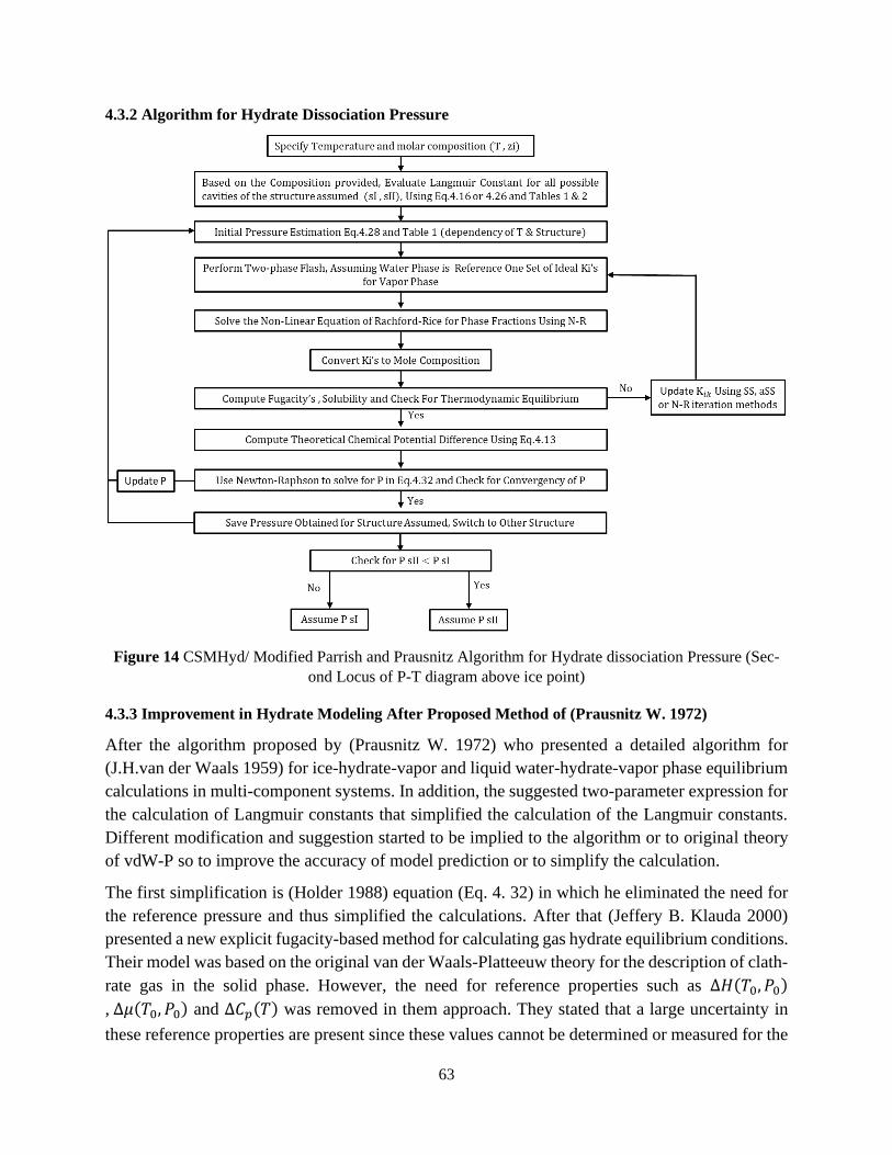
63

4.3.2 Algorithm for Hydrate Dissociation Pressure

Figure 14 CSMHyd/ Modified Parrish and Prausnitz Algorithm for Hydrate dissociation Pressure (Sec-

ond Locus of P-T diagram above ice point)

4.3.3 Improvement in Hydrate Modeling After Proposed Method of (Prausnitz W. 1972)

After the algorithm proposed by (Prausnitz W. 1972) who presented a detailed algorithm for

(J.H.van der Waals 1959) for ice-hydrate-vapor and liquid water-hydrate-vapor phase equilibrium

calculations in multi-component systems. In addition, the suggested two-parameter expression for

the calculation of Langmuir constants that simplified the calculation of the Langmuir constants.

Different modification and suggestion started to be implied to the algorithm or to original theory

of vdW-P so to improve the accuracy of model prediction or to simplify the calculation.

The first simplification is (Holder 1988) equation (Eq. 4. 32) in which he eliminated the need for

the reference pressure and thus simplified the calculations. After that (Jeffery B. Klauda 2000)

presented a new explicit fugacity-based method for calculating gas hydrate equilibrium conditions.

Their model was based on the original van der Waals-Platteeuw theory for the description of clath-

rate gas in the solid phase. However, the need for reference properties such as ∆𝐻(𝑇0, 𝑃0)

, ∆𝜇(𝑇0, 𝑃0) and ∆𝐶𝑝(𝑇) was removed in them approach. They stated that a large uncertainty in

these reference properties are present since these values cannot be determined or measured for the

64

empty hydrate lattice. Despite that, the model was built in a way that instead of calculating refer-

ence chemical potential differences between a theoretical hydrate lattice and actual hydrate lattices,

an actual fugacity of water in the hydrate lattice can be calculated directly. This fugacity was de-

fined as the product of the water fugacity in the empty hydrate lattice, and the exponential to the

(theoretical) chemical potential difference between the actual hydrate and the (pure) liquid water

phase as following:

Where −∆𝜇𝑤𝛽−𝐻

is defined in Eq.4.5 or 4.8 while 𝑓𝑤𝛽

was defined using Poynting factor by prop-

erties such as saturated water vapor pressure and its molar volume. Both of these properties were

assumed temperature- and pressure dependent. In addition, (Jeffery B. Klauda 2000) attributed for

the second and third water shells surrounding the guest in each cavity in the calculation of Lang-

muir constants. They claimed that model had not been “tuned” by fitting Langmuir parameters to

actual hydrate dissociation pressure data but actually they were calculated from the Kihara cell

potential with parameters found in the literature, where these had been estimated from gas phase

viscosity data or second virial coefficients. In other words, no tune to the model is made since the

measurement are accurate. In this study they have reported accurate prediction with a percent ab-

solute average deviation in the predicted equilibrium pressures of 3.27% with two or three guest-

hydrate specific parameters compared to more than 11% with three adjustable parameters in the

vdW-P type models and 8.55% using a thermodynamic model that uses five guest-hydrate param-

eters for methane, ethane, propane, cyclopropane, iso-butane, carbon dioxide, nitrogen and hydro-

gen sulfide. Unlike (Jeffery B. Klauda 2000), (A.L Ballard 2002) suggested an improvement of

the classical van der Waals- Platteeuw/Parrish-Prausnitz approach, but expanded the theory by

accounting for the non-ideality of hydrate and including and accounting for lattice distortion in the

form of an activity correction. In addition, (A.L Ballard 2002) proposed a new development of

fugacity much simpler to use. Why we are discussing that? The hydrate model and the parameters

presented by (A.L Ballard 2002) represent the approach adopted in CSMGem software.

4.4 Hydrate Model of Ballard 2002

(A.L Ballard 2002) Hydrate modeling carried out in CSMGem Software (Colorado School of Min-

eral)

4.4.1 Model Theory

(A.L Ballard 2002) Main modification was based on the fact that hydrates are non-ideal from a

thermodynamic point of view. They stated that the current vdW-P hydrate model based on the

statistical thermodynamics and classical thermodynamics is a good and acceptable model for mod-

erate temperature and pressure conditions. However, as today’s need of energy became greater in

which drilling and production is taking place from deep and ultra-deep water, the need for much

more accurate model is necessary. Based on that, (A.L Ballard 2002) made an improvement to the

𝑓𝑤𝐻 = 𝑓𝑤

𝛽. 𝑒𝑥𝑝 [

−∆𝜇𝑤𝛽−𝐻

𝑅. 𝑇] (4.33)

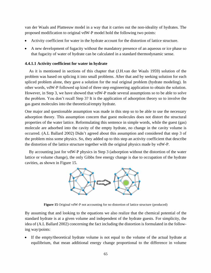
65

van der Waals and Platteeuw model in a way that it carries out the non-ideality of hydrates. The

proposed modification to original vdW-P model hold the following two points:

• Activity coefficient for water in the hydrate account for the distortion of lattice structure.

• A new development of fugacity without the mandatory presence of an aqueous or ice phase so

that fugacity of water of hydrate can be calculated in a standard thermodynamic sense.

4.4.1.1 Activity coefficient for water in hydrate

As it is mentioned in sections of this chapter that (J.H.van der Waals 1959) solution of the

problem was based on splicing it into small problems. After that and by seeking solution for each

spliced problem alone, they gave a solution for the real original problem (hydrate modeling). In

other words, vdW-P followed up kind of three step engineering application to obtain the solution.

However, in Step 3, we have showed that vdW-P made several assumptions so to be able to solve

the problem. You don’t recall Step 3? It is the application of adsorption theory so to involve the

gas guest molecules into the theoretical/empty hydrate.

One major and questionable assumption was made in this step so to be able to use the necessary

adsorption theory. This assumption concern that guest molecules does not distort the structural

properties of the water lattice. Reformulating this sentence in simple words, while the guest (gas)

molecule are adsorbed into the cavity of the empty hydrate, no change in the cavity volume is

occurred. (A.L Ballard 2002) Didn’t agreed about this assumption and considered that step 3 of

the problem miss some physics. So, they added up to this step an activity coefficient that describe

the distortion of the lattice structure together with the original physics made by vdW-P.

By accounting just for vdW-P physics in Step 3 (adsorption without the distortion of the water

lattice or volume change), the only Gibbs free energy change is due to occupation of the hydrate

cavities, as shown in Figure 15.

Figure 15 Original vdW-P not accounting for no distortion of lattice structure (produced)

By assuming that and looking to the equations we also realize that the chemical potential of the

standard hydrate is at a given volume and independent of the hydrate guests. For simplicity, the

idea of (A.L Ballard 2002) concerning the fact including the distortion is formulated in the follow-

ing way/points:

• If the empty/theoretical hydrate volume is not equal to the volume of the actual hydrate at

equilibrium, that mean additional energy change proportional to the difference in volume

66

should be added. How It can be added without reformulating the problem?

• Ans: add an activity coefficient account for the change of volume so to correct Gibbs free

energy obtained by vdW-P theory.

(A.L Ballard 2002) Model is illustrated in the figure below

Figure 16 (A.L Ballard 2002) Modified model accounting for distortion of lattice structure (produced)

Rewriting Eq. (4. 5) for chemical potential difference between hydrate and empty hydrate and

including the distortion term of Ballard and Sloan we obtain:

Where 𝑙𝑛 𝛾𝑤𝐻 is activity coefficient accounting for the perturbation of Gibbs energy due to volume

change expressed as following:

Where (A.L Ballard 2002) arbitrarily defined the perturbed potential or Gibbs energy and enthalpy

of formation to be linear in ∆𝑉𝐻 such as ∆𝑔𝑤0𝛽 = a∆𝑣𝑣𝐻0 and ∆𝑣ℎ𝑤0𝛽 = 𝑏∆𝑣𝑣𝐻0

using parame-

ters:

Table 5 Formation properties of empty hydrate

Hydrate 𝒈𝒘𝟎𝜷 (J/mole) 𝒉𝒘𝟎𝜷 (J/mole) a (J/ cm3 ) b (J/cm3)

sI -235537.85 -291758.77 25.74 -481.32

sII -235627.53 -292044.10 260.00 -68.64

sH -235491.02 -291979.26 0 0

4.4.1.2 Fugacity development

(A.L Ballard 2002) Insisted that there is a major barrier in the fugacity equation of water in hydrate.

In order to compute fugacity of water in hydrate using Eq. (4. 33), firstly fugacity of water in

empty hydrate need to calculate using:

∆𝜇(𝑇, 𝑃, 𝜃)𝑤𝐻−𝛽

= 𝑅. 𝑇.∑[𝑣𝑚 . ln (1 − ∑𝜃(𝑇, 𝑃, �̅�)𝑚.𝑗

𝑗

)]

𝑚

+ 𝑙𝑛 𝛾𝑤𝐻 (4.34)

∆𝑣𝑔𝑤𝛽

𝑅. 𝑇=

∆𝑣𝑔𝑤0𝛽

𝑅. 𝑇0− ∫

∆𝑣ℎ𝑤𝛽

𝑅. 𝑇2

𝑇

𝑇0

𝑑𝑇 + ∫∆𝑣𝑣𝐻

𝑅. 𝑇

𝑃

𝑃0

. 𝑑𝑃 (4.35)

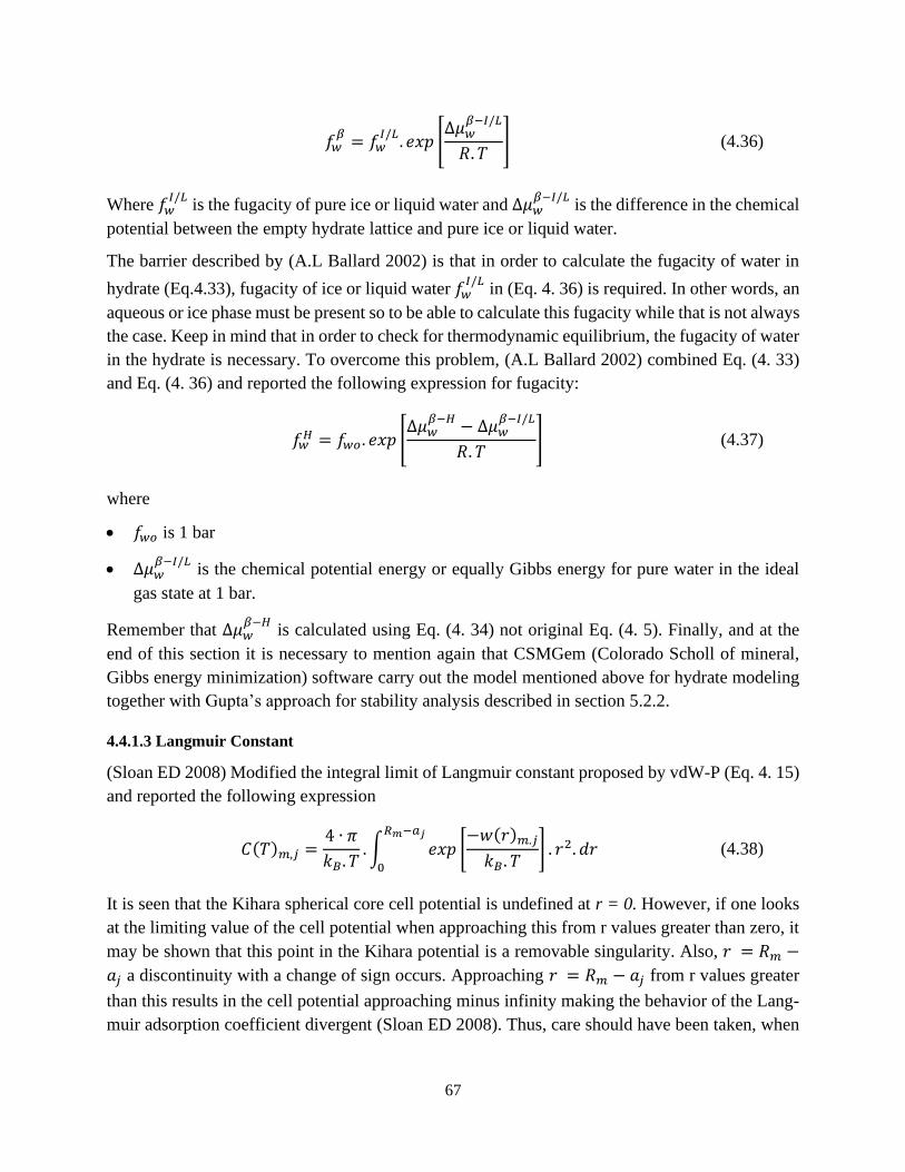
67

Where 𝑓𝑤𝐼/𝐿

is the fugacity of pure ice or liquid water and ∆𝜇𝑤𝛽−𝐼/𝐿

is the difference in the chemical

potential between the empty hydrate lattice and pure ice or liquid water.

The barrier described by (A.L Ballard 2002) is that in order to calculate the fugacity of water in

hydrate (Eq.4.33), fugacity of ice or liquid water 𝑓𝑤𝐼/𝐿

in (Eq. 4. 36) is required. In other words, an

aqueous or ice phase must be present so to be able to calculate this fugacity while that is not always

the case. Keep in mind that in order to check for thermodynamic equilibrium, the fugacity of water

in the hydrate is necessary. To overcome this problem, (A.L Ballard 2002) combined Eq. (4. 33)

and Eq. (4. 36) and reported the following expression for fugacity:

where

• 𝑓𝑤𝑜 is 1 bar

• ∆𝜇𝑤𝛽−𝐼/𝐿

is the chemical potential energy or equally Gibbs energy for pure water in the ideal

gas state at 1 bar.

Remember that ∆𝜇𝑤𝛽−𝐻

is calculated using Eq. (4. 34) not original Eq. (4. 5). Finally, and at the

end of this section it is necessary to mention again that CSMGem (Colorado Scholl of mineral,

Gibbs energy minimization) software carry out the model mentioned above for hydrate modeling

together with Gupta’s approach for stability analysis described in section 5.2.2.

4.4.1.3 Langmuir Constant

(Sloan ED 2008) Modified the integral limit of Langmuir constant proposed by vdW-P (Eq. 4. 15)

and reported the following expression

It is seen that the Kihara spherical core cell potential is undefined at r = 0. However, if one looks

at the limiting value of the cell potential when approaching this from r values greater than zero, it

may be shown that this point in the Kihara potential is a removable singularity. Also, 𝑟 = 𝑅𝑚 −

𝑎𝑗 a discontinuity with a change of sign occurs. Approaching 𝑟 = 𝑅𝑚 − 𝑎𝑗 from r values greater

than this results in the cell potential approaching minus infinity making the behavior of the Lang-

muir adsorption coefficient divergent (Sloan ED 2008). Thus, care should have been taken, when

𝑓𝑤𝛽

= 𝑓𝑤𝐼/𝐿

. 𝑒𝑥𝑝 [∆𝜇𝑤

𝛽−𝐼/𝐿

𝑅. 𝑇] (4.36)

𝑓𝑤𝐻 = 𝑓𝑤𝑜 . 𝑒𝑥𝑝 [

∆𝜇𝑤𝛽−𝐻

− ∆𝜇𝑤𝛽−𝐼/𝐿

𝑅. 𝑇] (4.37)

𝐶(𝑇)𝑚,𝑗 =4 ∙ 𝜋

𝑘𝐵. 𝑇.∫ 𝑒𝑥𝑝 [

−𝑤(𝑟)𝑚.𝑗

𝑘𝐵. 𝑇]

𝑅𝑚−𝑎𝑗

0

. 𝑟2. 𝑑𝑟 (4.38)

68

integrating the Kihara cell potential in CSMGem. Additionally, different optimized Kihara param-

eter have been used than the one reported by (Prausnitz W. 1972) and used in CSMHyd.

Table 6 Kihara Parameters reported by (Sloan ED 2008) used in CSMGem

Component 𝒂𝒋 (A) σ (A) ε/k (K)

Methane 0.3834 3.14393 155.593

Ethane 0.5651 3.24693 188.181

Propylene 0.6500 3.33039 186.082

Propane 0.6502 3.41670 192.855

n-Butane 0.9379 3.51726 197.254

i-Butane 0.8706 3.41691 198.333

i-Pentane 0.9868 3.54550 199.560

Nitrogen 0.3526 3.13512 127.426

Hydrogen Sulfide 0.3600 3.10000 212.047

Carbon Dioxide 0.6805 2.97638 175.405

4.5 MultiFlash and HydraFLASH® Hydrate Modelling

Hydrate modeling carried out in HydraFLASH® and MultiFlash Software

4.5.1 Model Theory

In both software, modeling of hydrates is based on the original vdW-P theory. However, this model

is employed to calculate the fugacity coefficient of water in hydrate phase so to be used for ther-

modynamic equilibrium purposes. Both fugacity of water in hydrate and in empty hydrates are

calculated and expressed in the same form as Eq. 4. 33 and 4. 36 respectively. In addition, Lang-

muir constant in HydraFLASH is calculated by adopting Eq. (4.38) with the following Kihara

parameters (Tohidi-Kalorazi 1995) and used again in optimization of Kihara parameters for alco-

hols from the same institute in 2009 are as following:

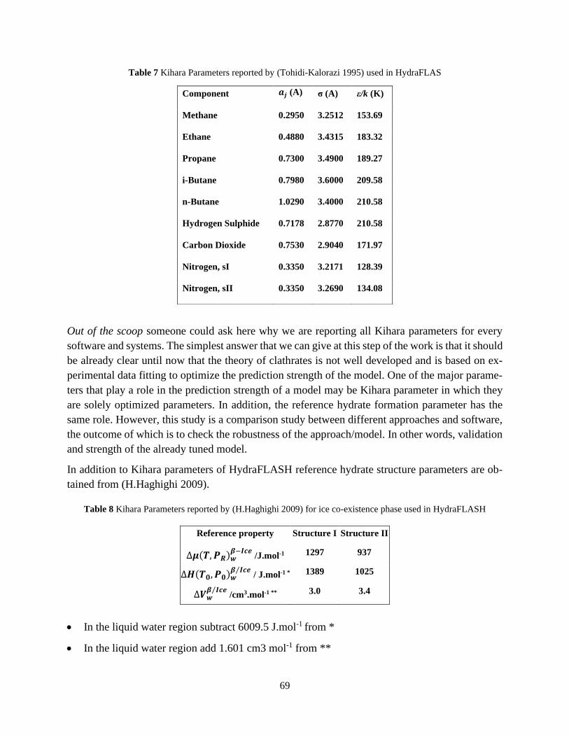
69

Table 7 Kihara Parameters reported by (Tohidi-Kalorazi 1995) used in HydraFLAS

Out of the scoop someone could ask here why we are reporting all Kihara parameters for every

software and systems. The simplest answer that we can give at this step of the work is that it should

be already clear until now that the theory of clathrates is not well developed and is based on ex-

perimental data fitting to optimize the prediction strength of the model. One of the major parame-

ters that play a role in the prediction strength of a model may be Kihara parameter in which they

are solely optimized parameters. In addition, the reference hydrate formation parameter has the

same role. However, this study is a comparison study between different approaches and software,

the outcome of which is to check the robustness of the approach/model. In other words, validation

and strength of the already tuned model.

In addition to Kihara parameters of HydraFLASH reference hydrate structure parameters are ob-

tained from (H.Haghighi 2009).

Table 8 Kihara Parameters reported by (H.Haghighi 2009) for ice co-existence phase used in HydraFLASH

• In the liquid water region subtract 6009.5 J.mol-1 from *

• In the liquid water region add 1.601 cm3 mol-1 from **

Component 𝒂𝒋 (A) σ (A) ε/k (K)

Methane 0.2950 3.2512 153.69

Ethane 0.4880 3.4315 183.32

Propane 0.7300 3.4900 189.27

i-Butane 0.7980 3.6000 209.58

n-Butane 1.0290 3.4000 210.58

Hydrogen Sulphide 0.7178 2.8770 210.58

Carbon Dioxide 0.7530 2.9040 171.97

Nitrogen, sI 0.3350 3.2171 128.39

Nitrogen, sII 0.3350 3.2690 134.08

Reference property Structure I Structure II

∆𝝁(𝑻, 𝑷𝑹)𝒘𝜷−𝑰𝒄𝒆

/J.mol-1 1297 937

∆𝑯(𝑻𝟎, 𝑷𝟎)𝒘𝜷 𝑰𝒄𝒆⁄

/ J.mol-1 * 1389 1025

∆𝑽𝒘𝜷 𝑰𝒄𝒆⁄

/cm3.mol-1 **

3.0 3.4

70

And ∆𝐶𝑝(𝑇) 𝑖𝑛 (𝐸𝑞 4.26) is reported differently than (Prausnitz W. 1972) as following:

A very important Note: all hydrate models have more or less the same basis and they all rely on

the theory of van der Waals- Platteeuw a good example of that is HydraFLASH and MultiFlash.

However, what differentiates the strength of prediction from one to other is the tuning procedure

and experimental data used. For example, and at this part of this work, we will give you a hint:

one of the software/approaches could accurately predict in a specific locus of incipient hydrate

dissociation (e.g. Lw-H-V) while in another locus it will poorly predict. Another approach could

work in the opposite way while no change in basis theory is present. This fact can be explained on

the fact that while tuning an approach frequent experimental data originally located in the same

locus (good prediction) are used than any other. Why we are mentioning that? Here is a quick

answer, data is money in our case the data are the experimental points used to tune and money is

the business software present in the market. How that is related to the topic above? Kihara param-

eters and reference hydrate structure parameters are the Keys of increasing the balance amount of

company’s providing the software and since we are living in a capitalism world, no one will give

you the key to gain money and sacrifice his own business or even to be in the danger zone of that.

Based on that, unfortunately we haven’t managed yet to obtain the Keys of KBC/MultiFlash Com-

pany. In other words, Kihara parameters and all other tuned parameters are still unaccusable. How-

ever, we will keep digging trying to find the keys.

∆𝐶𝑝(𝑇) = −37.32 + 0.179(𝑇 − 273.15) (4.39)

71

Chapter 5

5 Thermodynamic Models

Studying thermodynamics of hydrates rigorously was initially attempted in 1959 by van der Waals

and Platteeuw. This innovative study attempt initiated the process that led to the development of

several tools/approaches enabling the analysis of complex systems (e.g. CO2) later on. Nowadays,

the approaches enable both understanding of hydrates and the efficient development in flow assur-

ance in the oil and gas industries. In their model, VdW-P took advantage of Langmuir adsorption

theory to describe guest molecules adsorption in a theoretical empty hydrate. While some of the

approaches present today adopted the original theory of vdW-P, others, questioned an assumption

present in the theory basis. This assumption describes guest molecules adsorption in the empty

theoretical hydrate (defined by VdW-P). In this, it is stated that guest molecules make no distortion

of the theoretical empty hydrate lattice structure. (A.L Ballard 2002) eliminated this questionable

assumption by adding an activity coefficient to the original theory of VdW-P. The activity coeffi-

cient covers only the distortion factor in the empty hydrate structure. On the other hand, different

approaches took advantage of the ability of CPA (Cubic Plus Association) EoS in modeling hy-

drogen bonding. Others use simple cubic EoS (e.g. SRK) to model polar components (e.g. water).

Additionally, in each of these approaches, several thermodynamic tools have been used for differ-

ent descriptions of different possible hydrates co-existing phases (e.g. ice).

In Chapter 2, the formulation of a phase equilibria problem using Two and Multiphase systems is

shown. The first outcome of which is that material balance (M.B) and thermodynamics are com-

bined to describe the real problem. Typically, the thermodynamic constraint is satisfied or re-

spected when all fugacity of each component at all phases are equal.

In Chapter 4, the fugacity calculation of water in hydrates is discussed in detail. In other words,

the fugacity model of water in hydrate is already present. But what about other phases (vapor,

ice…)? In the procedure explained in Chapter 2, it is assumed that the tools and relationships of

different models used to check for thermodynamic equilibrium exist. If so, what are these tools

and how they are correlated to the intensive properties of interest?

In this chapter, the discussion will be mainly based on different thermodynamic models and aux-

iliary functions used to simplify Gibbs equations for equilibrium (e.g. fugacity, activity coeffi-

cient). Keeping in mind that this study is a comparison between different software/approaches, so

it is evident to know each approach or software adopted models for each phase treatment and

calculation. With that, a better understanding of the algorithm behavior in each software will be

decelerated. Consequently, a much accurate analysis of results can be made. Based on that, the end

of this chapter will be providing a summary of this information.

In a typical petroleum system and under the assumption that the system will split and form more

than one phase at equilibrium, vapor gas hydrocarbons, and liquid hydrocarbons will be present.

72

However, in some rare cases of high carbon dioxide concentration and due to the non-ideal behav-

ior of this component, carbon dioxide can be present in both liquid and vapor phases. Additionally,

the hydrate system at equilibrium may be formed with several co-existent phases such as Ice, Liq-

uid water, vapor hydrocarbons, and liquid hydrocarbons. Also, other phases and components can

be present in hydrate such as salts, alcohols, glycols. In a typical industrial case, both alcohols and

salts can be present simultaneously. The last case can be present in a system of a pipeline connect-

ing directly offshore gas production to the onshore. Offshore gas platforms are limited space plat-

forms so while producing gas and especially in cases of huge reserves (e.g. Offshore Zohr Egypt),

due to the limited spaces of platforms no storage of produced gas will take place. The gas will be

directly sent onshore through a pipeline. However, since gas stream trajectory start from the res-

ervoir following well-pipes to transport pipelines and keeping in mind that the gas is produced

from reservoir formation in which saline water is present (average order of 350,000 ppm) while

no treatment of water that will take place at the platform, a significant (Water-aquifers presence)

to negligible amount of saline water is present within the gas phase in pipeline. Based on this fact,

the only remained solution to avoid the risk of hydrate blockage, in this case, is thermodynamic

inhibitors injection. As a conclusion, the typical (real-life) industrial case will include salts, alco-

hols, vapor hydrocarbons and probably liquid hydrocarbon too in a state of high concentration of

light components and finally aqueous phase. Thus it is essential to know how to model each phase

that may be present in the system.

What has been stated conclude the major objective of this chapter. However, at this point, this

chapter will present the major tools for the main phases of forming hydrates where salts and in-

hibitors’ models will not be explained. Salts (Electrolytes) modeling and inhibitors will be ex-

plained separately in a different chapter within the results of this study for each mentioned phase.

Fugacity was defined by the thermodynamics G. N. Lewis, this property is better understood by

engineers and physically felt than abstraction chemical potential. We have used fugacity to get

around the mathematical anomalies faced in solving the phase equilibria problem. Fugacity is de-

fined inductively while other thermodynamic parameters are defined deductively. For example,

enthalpy is developed by combining internal energy and flow work of the system while fugacity

definition started with an ideal/real gas which later is extended to the liquid and solid phase. Fu-

gacity is the parameter that replaced pressure due non-ideality of molecules of the phase. It is

known that intermolecular forces of gases cause deviations of the gas from ideality, in which the

behavior is called real gas behavior. To describe ideal gas, fugacity and pressure both can be used

correspondingly while in real gas systems, only fugacity is used.

5.1 Vapor Phase

Reliable thermodynamic data is required in advance to obtain fugacity for pure real gas through

thermodynamic tables, equation of state or generalized correlations. For the need of one fugacity

value, fugacity tables are the best method to be used where thermodynamic tables are based on

reliable experimental work. However, that is not the case in this problem (Hydrate, Petroleum). In

reality and both areas, we don’t expect to encounter a pure real gas. Additionally, in different

73

algorithm sections, iteration techniques are required to achieve the correct answer or the global

minimum of Gibbs energy thus the table’s values cannot be relied on.

For any engineer, algorithm scientist or software engineer a relationship that correlates fugacity to

all dependent parameters would be ideal. This relationship is provided by the use of already present

cubic EoSs. However, to use EoS in obtaining fugacity-coefficient for a component i in a mixture,

the need to describe PvT Property’s behavior for that mixture is necessary. Unlike pure compo-

nents which are described experimentally, the need for mixture rules such as van-der-Waals rules

is the only solution to overcome this problem.

The theoretical justification of mixture rules is so limited. A mixture rule works perfectly in de-

scribing a certain mixture or fluid while for another one is not necessarily true. Despite that now,

this work does not involve studying the effect of mixture rules on the prediction of our models/ap-

proaches.

Starting by Eq. (2. 5) 𝜇𝑖 − 𝜇𝑖0 = 𝑅𝑇 ln [

𝑓�̂�

𝑓𝑖�̂�]

where

• 𝜇𝑖 is the chemical potential for pressure, temperature, and composition of interest.

• 𝜇𝑖0 is the chemical potential for chosen reference at the same temperature and composition of

the mixture at low pressure (this one is criteria for the definition of fugacity and is discussed

down why such a reference state is chosen).

To correlate fugacity within an EoS, the partial derivative relation of Gibbs energy is substituted

in Eq. (2. 5)

For detailed substitution search for “Relations among Partial Molar Quantities”. By looking at

Εquation 5.1, a volume explicit equation of state is required. This is not the case with typical EoS

where they are pressure explicit equations. To overcome this issue, Eq. (5. 1) is to be rewritten so

that to use typical pressure explicit EoS. To do so first recalling the definition of partial molar

property

using the well-known cyclic rule at constant T

𝜇𝑖 − 𝜇𝑖0 = ∫ 𝑉�̅�𝑑𝑃

𝑃

𝑃𝑙𝑜𝑤

= 𝑅𝑇 ln [𝑓𝑖

𝑣

𝑦𝑖𝑃𝑙𝑜𝑤] (5.1)

𝑉�̅� = (𝜕𝑉

𝜕𝑛𝑖)

𝑇,𝑃,𝑛𝑗≠𝑖

(5.2)

(𝜕𝑉

𝜕𝑛𝑖)

𝑇,𝑃

(𝜕𝑃

𝜕𝑉)

𝑇,𝑛𝑖

(𝜕𝑛𝑖

𝜕𝑃)

𝑇,𝑉= −1 (5.3)

74

Since we have chosen the reference phase to be identical in temperature and composition, cyclic

rule in Eq. (5. 3) can be written as:

substituting (5. 4) into (5. 1)

Finally, using Eq. (5. 5) fugacity is formulated within a cubic pressure explicit EoS.

Note: In this work, it is purposely avoided discussing the fundamentals of thermodynamic to keep

the track mainly and solely from an engineering point of view.

Obtaining Eq. (5. 5) and by choosing a reliable cubic equation of state, describing the fugacity

explicitly is now much easier. Several cubic equations of state (EoS) are used in both areas hydrate

and petroleum for vapor phase treatment. However, the two well-known equations of state for

which several publications came out and dozens of the authors agreed on are Peng Robinson (PR-

EOS-1976) and Soave-Redlich-Kwong (SRK-EoS-1972) which give the best prediction in petro-

leum field (e.g. VLEP). One of these two equations can be chosen for the calculations needed.

Additionally, this study involves the effect of cubic EoS type on hydrate prediction in which until

now no one has studied/reported this effect. At this phase, to this point, just a general idea of EoS

has been given. However, this study includes the effect of EoS choice on hydrate prediction accu-

racy, a short description of cubic EoS will be given later. At this stage of the calculations and for

simplicity reasons, van-der-Waals equation of state with simple mixture rules are chosen to de-

scribe obtaining explicit fugacity relationship, using EoS as following:

where

• 𝑎𝑚𝑖𝑥 Is the attraction term covers the intermolecular forces between molecules and is depend-

ent on the gas molecules present.

• 𝑏𝑚𝑖𝑥 Is the co-volume excluded term and is related to the size of molecules.

As it is mentioned above that each of the parameters is related to a specific molecule. When it

comes to mixtures simple mixture rules are assumed since no molecular theory can describe men-

tioned parameters for mixtures. Using qualitative molecular description combined with mathemat-

ical simple averaging van-der-Waals proposed the following description of 2 mixtures (a and b):

(𝜕𝑉

𝜕𝑛𝑖)

𝑇,𝑃

𝑑𝑃 = −(𝜕𝑃

𝜕𝑛𝑖)

𝑇,𝑉

𝑑𝑉 (5.4)

𝑅𝑇 ln [𝑓𝑖

𝑣

𝑦𝑖𝑃𝑙𝑜𝑤] = −∫ (

𝜕𝑃

𝜕𝑛𝑖)

𝑇,𝑃,𝑛𝑗≠𝑖

𝑑𝑉 𝑉

(𝑛𝑇𝑅𝑇𝑃𝑙𝑜𝑤

)

(5.5)

𝑃 =𝑅𝑇

𝑣 − 𝑏𝑚𝑖𝑥−

𝑎𝑚𝑖𝑥

𝑣2 (5.6)

75

in which

where

• 𝑎𝑖𝑖 represents the attraction between like i molecules

• 𝑎𝑖𝑗 represents the interaction between one i molecule and one j molecule, the unlikely interac-

tion.

However, when more data are present the empirical fitting parameter 𝑘𝑖𝑗 is obtained for better

prediction.

In some cases, this binary interaction parameter is used as a tuning parameter for better prediction

of EoS and a better prediction of reservoir fluid PvT properties.

For the size 𝑏𝑚𝑖𝑥 parameter, it is most convenient to average molecular volumes as follows:

Now after discussing all of this let’s go back to Eq. (5. 5) and derive an equation for fugacity using

Eq. (5. 6).

For more simplicity, let’s assume a binary mixture compound of components a and b. Starting by

rewriting Eq. (5. 5) for the binary mixture described

rewriting Eq. (5. 6) for the same mixture

in addition to Eq. (5. 7), (5. 10)

𝑎𝑚𝑖𝑥 = ∑∑𝑦𝑖𝑦𝑗𝑎𝑖𝑗 (5.7)

𝑎𝑖𝑗 = √𝑎𝑖𝑖𝑎𝑗𝑗 (5.8)

𝑎𝑖𝑗 = √𝑎𝑖𝑖𝑎𝑗𝑗 (1 − 𝑘𝑖𝑗) (5.9)

𝑏𝑚𝑖𝑥 = ∑𝑦𝑖𝑏𝑖 (5.10)

𝑅𝑇 ln [𝑓𝑎

𝑣

𝑦𝑎𝑃𝑙𝑜𝑤] = −∫ (

𝜕𝑃

𝜕𝑛𝑎)𝑉,𝑇,𝑛𝑏

𝑉

(𝑛𝑇𝑅𝑇𝑃𝑙𝑜𝑤

)

𝑑𝑉 (5.11)

𝑃 =𝑅𝑇(𝑛𝑎 + 𝑛𝑏)

𝑉 − (𝑛𝑎𝑏𝑎 + 𝑛𝑏𝑏𝑏)−

𝑛𝑎2𝑎𝑎 + 2𝑛𝑎𝑛𝑏√𝑎𝑎𝑎𝑏 + 𝑛𝑏

2𝑎𝑏

𝑣2 (5.12)

76

and applying the mass balance

deriving (5. 12)

substituting (5. 12) into (5. 11)

Simplification can be made to Eq. (5.17) on the following basis 𝑅𝑇

𝑃𝑙𝑜𝑤 >> 𝑏𝑚𝑖𝑥 , adding 𝑙𝑛(𝑃𝑙𝑜𝑤)

to both sides and considering that 𝑃𝑙𝑜𝑤 tends to 0, Eq (5.17) becomes:

Subtracting ln(P) from both sides’ leaves:

An explicit equation of fugacity using cubic EoS correlating all intensive properties of interest is

already formulated. The following table summarizes the fugacity coefficient for three cubic equa-

tio

𝑎𝑚𝑖𝑥 = 𝑦𝑎2𝑎𝑎 + 2𝑦𝑎𝑦𝑏√𝑎𝑎𝑎𝑏 + 𝑦𝑏

2𝑎𝑏 (5.13)

𝑏𝑚𝑖𝑥 = 𝑦𝑎𝑏𝑎 + 𝑦𝑏𝑏𝑏 (5.14)

𝑛𝑇 = 𝑛𝑎 + 𝑛𝑏 (5.15)

(𝜕𝑃

𝜕𝑛𝑎)

𝑇,𝑉,𝑛𝑏

=𝑅𝑇

𝑉 − (𝑛𝑎𝑏𝑎 + 𝑛𝑏𝑏𝑏)+

𝑏𝑎𝑅𝑇(𝑛𝑎 + 𝑛𝑏)

[𝑉 − (𝑛𝑎𝑏𝑎 + 𝑛𝑏𝑏𝑏)]2

−2(𝑛𝑎𝑎𝑎 + 𝑛𝑏√𝑎𝑎𝑎𝑏)

𝑉2

(5.16)

ln [𝑓𝑎

𝑣

𝑦𝑎𝑃𝑙𝑜𝑤] = − ln [

𝑉 − 𝑛𝑇𝑏𝑚𝑖𝑥

(𝑛𝑇𝑅𝑇𝑃𝑙𝑜𝑤

) − 𝑛𝑇𝑏𝑚𝑖𝑥

] +𝑏𝑎(𝑛𝑎 + 𝑛𝑏)

[𝑉 − 𝑛𝑇𝑏𝑚𝑖𝑥]−

𝑏𝑎(𝑛𝑎 + 𝑛𝑏)

[(𝑛𝑇𝑅𝑇𝑃𝑙𝑜𝑤

) − 𝑛𝑇𝑏𝑚𝑖𝑥]

−2(𝑛𝑎𝑎𝑎 + 𝑛𝑏√𝑎𝑎𝑎𝑏)

𝑅𝑇𝑉+

2(𝑛𝑎𝑎𝑎 + 𝑛𝑏√𝑎𝑎𝑎𝑏)

𝑅𝑇 (𝑛𝑇𝑅𝑇𝑃𝑙𝑜𝑤

)

(5.17)

ln [𝑓𝑎

𝑣

𝑦𝑎] = − ln [

(𝑉 − 𝑛𝑇𝑏𝑚𝑖𝑥)

𝑛𝑇𝑅𝑇] +

𝑏𝑎(𝑛𝑎 + 𝑛𝑏)

[𝑉 − 𝑛𝑇𝑏𝑚𝑖𝑥]

−2(𝑛𝑎𝑎𝑎 + 𝑛𝑏√𝑎𝑎𝑎𝑏)

𝑅𝑇𝑉

(5.18)

ln [𝑓𝑎

𝑣

𝑦𝑎𝑃] = ln[�̂�𝑎

𝑣] = − ln𝑃(𝑣 − 𝑏𝑚𝑖𝑥)

𝑅𝑇+

𝑏𝑎

[𝑣 − 𝑏𝑚𝑖𝑥]−

2(𝑦𝑎𝑎𝑎 + 𝑦𝑏√𝑎𝑎𝑎𝑏)

𝑅𝑇𝑣 (5.19)

77

Table 9 Fugacity coefficient for three cubic EoS

Van der Waals

Equation of state

Pure component i 𝒍𝒏𝝋𝒊 =𝒃𝒊

𝒗𝒊 − 𝒃𝒊

− 𝒍𝒏((𝒗𝒊 − 𝒃𝒊)𝑷

𝑹𝑻) −

𝟐𝒂𝒊

𝑹𝑻𝒗𝒊

(5.20)

Component i in a

binary mixture. 𝒍𝒏𝝋�̂� =

𝒃𝟏

𝒗 − 𝒃− 𝒍𝒏(

(𝒗 − 𝒃)𝑷

𝑹𝑻) −

𝟐(𝒚𝟏𝒂𝟏 + 𝒚𝟐𝒂𝟏𝟐)

𝑹𝑻𝒗 (5.21)

Species i in a mixture 𝒍𝒏𝝋�̂� =𝒃𝒊

𝒗 − 𝒃− 𝒍𝒏(

(𝒗 − 𝒃)𝑷

𝑹𝑻) −

𝟐∑ 𝒚𝟏𝒂𝒊𝒌𝒎𝒌=𝟏

𝑹𝑻𝒗 (5.22)

Redlich-Kwong

Equation of State

Pure component 𝐥𝐧𝝋𝒊 = 𝒛𝒊 − 𝟏 − 𝐥𝐧((𝒗𝒊 − 𝒃𝒊)𝑷

𝑹𝑻) −

𝒂𝒊

𝒃𝒊𝑹𝑻𝟏.𝟓𝐥𝐧 (𝟏 +

𝒃𝒊

𝒗𝒊

) (5.23)

Component i in a

binary mixture

𝑙𝑛 𝜑1̂ =𝑏1

𝑏(𝑧 − 1) − ln (

(𝑣 − 𝑏)𝑃

𝑅𝑇)

+1

𝑏𝑅𝑇1.5[𝑎𝑏1

𝑏− 2(𝑦1𝑎1 + 𝑦2𝑎12)] ln (1 +

𝑏

𝑣)

(5.24)

Species i in a mixture 𝒍𝒏𝝋�̂� =𝒃𝟏

𝒃(𝒛 − 𝟏) − 𝒍𝒏(

(𝒗 − 𝒃)𝑷

𝑹𝑻) +

𝟏

𝒃𝑹𝑻𝟏.𝟓[𝒂𝒃𝟏

𝒃− 𝟐∑ 𝒚𝟏𝒂𝒊𝒌

𝒎

𝒌=𝟏

] 𝒍𝒏 (𝟏 +𝒃

𝒗) (5.25)

Peng Robinson

Equation of State -

Pure component i 𝐥𝐧𝝋𝒊 = 𝒛𝒊 − 𝟏 − 𝐥𝐧((𝒗𝒊 − 𝒃𝒊)𝑷

𝑹𝑻) −

(𝒂𝜶)𝒊

𝟐√𝟐𝒃𝒊𝑹𝑻𝐥𝐧 [

𝒗𝒊 + (𝟏 + √𝟐)𝒃𝒊

𝒗𝒊 + (𝟏 − √𝟐)𝒃𝒊

] (5.26)

Component 1 in a

binary mixture

𝒍𝒏𝝋�̂� =𝒃𝟏

𝒃(𝒛 − 𝟏) − 𝒍𝒏 (

(𝒗 − 𝒃)𝑷

𝑹𝑻)

+𝒂𝜶

𝟐√𝟐𝒃𝑹𝑻[𝒃𝟏

𝒃

−𝟐

𝒂𝜶(𝒚𝟏(𝒂𝜶)𝟏 + 𝒚𝟐(𝒂𝜶)𝟏𝟐)] 𝐥𝐧 [

𝒗 + (𝟏 + √𝟐)𝒃

𝒗 + (𝟏 − √𝟐)𝒃]

(5.27)

Species i in a mixture

𝒍𝒏 𝝋�̂� =𝒃𝒊

𝒃(𝒛 − 𝟏) − 𝒍𝒏 (

(𝒗 − 𝒃)𝑷

𝑹𝑻)

+𝒂𝜶

𝟐√𝟐𝒃𝑹𝑻[𝒃𝟏

𝒃−

𝟐

𝒂𝜶∑ 𝒚𝒌(𝒂𝜶)𝒊𝒌

𝒎

𝒌=𝟏

] 𝐥𝐧 [𝒗 + (𝟏 + √𝟐)𝒃

𝒗 + (𝟏 − √𝟐)𝒃]

(5.28)

78

5.2 Liquid Hydrocarbon Phase

It should be clear that thermodynamic equilibrium is achieved when all components’ fugacity val-

ues in different phases present are equal. In other words, the component tendency of escaping is

the same in all phases. However, in the last section (5. 1), a detailed description is presented on

the way of obtaining the fugacity or fugacity coefficient for components present in the vapor phase

using EoS. Based on that a part of the problem is already solved regarding the vapor phase.

Now considering the liquid phase, a summarized equation for fugacity coefficient can be used to

describe it in this state

where

• 𝜑𝑖 is the fugacity coefficient of interest i.

• 𝛾𝑖 is the activity coefficient of component i.

• 𝑝𝑖𝑠𝑎𝑡 is the saturated vapor pressure of component i.

• 𝑝 is the total pressure.

• 𝛱𝑖 is Poynting correction.

in which ln 𝛾𝑖 is derived from the Excess Gibbs energy as follows:

However, the excess Gibbs energy at this stage of this work is not considered since EoS models

are used to calculate fugacity and not EoS with an activity coefficient. In other parts of this work

where salts/inhibitors are present, this term is necessarily tested in some approaches. In the hydro-

carbon liquid phase, this term is eliminated. The remained parts of the equation can be explained

using the knowledge already known for a petroleum engineer. To explain a P-v diagram is illus-

trated.(Figure 18).

Considering the equality of fugacity at equilibrium condition and applying that to the isotherm line

at saturation pressure

This equation is true for the blue points in the P-v diagram of a pure component at constant tem-

perature and pressure. But regarding the Fugacity of liquid, it is obtained at a pressure 𝑝𝑖 (red

point) through extrapolating fugacity value of the saturated liquid point (this part regarding liquid

phase fugacity is yet to be proved).

ln 𝜑𝑖 = ln 𝛾𝑖 + ln 𝑝𝑖𝑠𝑎𝑡 + ln𝜑𝑖

𝑠𝑎𝑡 − ln𝑝 + 𝛱𝑖 (5.29)

ln 𝛾𝑖 =𝜕𝐺𝐸

𝜕𝑛𝑖 (5.30)

𝑓𝑙𝑠𝑎𝑡 = 𝑓𝑣

𝑠𝑎𝑡 (5.31)

79

Figure 18 P-v diagram of a pure component

Rewriting fundamental Gibbs energy Equation (4. 21) for isothermal compression process

Integrating Eq. (5. 32) between pressure 𝑝𝑖 and 𝑝𝑖𝑠𝑎𝑡

Defining Gibbs energy for different state

&

Where ⌈(𝑇) is constant for the reference chosen (it is free to use any reference phase under some

conditions mentioned before). Despite that, Subtracting Eq. (5. 34) from (5. 35) and substituting

into (5.33) results in

𝑑𝐺 = 𝑉𝑑𝑃 (𝑐𝑜𝑛𝑠𝑡 𝑇) (5.32)

𝐺𝑖 − 𝐺𝑖𝑠𝑎𝑡 = ∫ 𝑉𝑖 𝑑𝑃

𝑃

𝑃𝑠𝑎𝑡

(5.33)

𝐺𝑖(𝑝𝑖) = ⌈(𝑇) + 𝑅𝑇 ln 𝑓𝑖 (5.34)

𝐺𝑖𝑠𝑎𝑡(𝑝𝑖

𝑠𝑎𝑡) = ⌈(𝑇) +𝑅𝑇 ln 𝑓𝑖𝑠𝑎𝑡

(5.35)

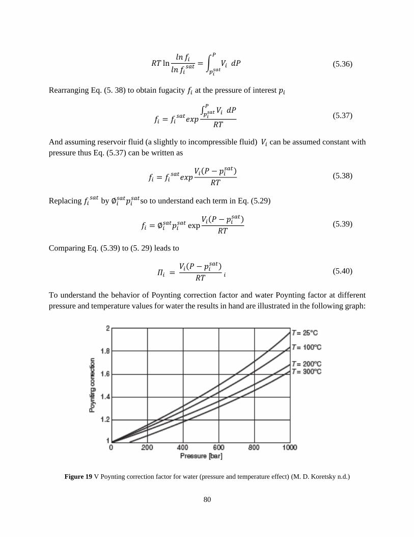
80

Rearranging Eq. (5. 38) to obtain fugacity 𝑓𝑖 at the pressure of interest 𝑝𝑖

And assuming reservoir fluid (a slightly to incompressible fluid) 𝑉𝑖 can be assumed constant with

pressure thus Eq. (5.37) can be written as

Replacing 𝑓𝑖𝑠𝑎𝑡

by ∅𝑖𝑠𝑎𝑡𝑝𝑖

𝑠𝑎𝑡so to understand each term in Eq. (5.29)

Comparing Eq. (5.39) to (5. 29) leads to

To understand the behavior of Poynting correction factor and water Poynting factor at different

pressure and temperature values for water the results in hand are illustrated in the following graph:

Figure 19 V Poynting correction factor for water (pressure and temperature effect) (M. D. Koretsky n.d.)

𝑅𝑇 ln𝑙𝑛 𝑓𝑖

𝑙𝑛 𝑓𝑖𝑠𝑎𝑡 = ∫ 𝑉𝑖 𝑑𝑃

𝑃

𝑝𝑖𝑠𝑎𝑡

(5.36)

𝑓𝑖 = 𝑓𝑖𝑠𝑎𝑡𝑒𝑥𝑝

∫ 𝑉𝑖 𝑑𝑃𝑃

𝑝𝑖𝑠𝑎𝑡

𝑅𝑇 (5.37)

𝑓𝑖 = 𝑓𝑖𝑠𝑎𝑡𝑒𝑥𝑝

𝑉𝑖(𝑃 − 𝑝𝑖𝑠𝑎𝑡)

𝑅𝑇 (5.38)

𝑓𝑖 = ∅𝑖𝑠𝑎𝑡𝑝𝑖

𝑠𝑎𝑡 exp𝑉𝑖(𝑃 − 𝑝𝑖

𝑠𝑎𝑡)

𝑅𝑇 (5.39)

𝛱𝑖 = 𝑉𝑖(𝑃 − 𝑝𝑖

𝑠𝑎𝑡)

𝑅𝑇 𝑖 (5.40)

81

As shown in figure 5.2 that Poynting correction factor at high pressure and low temperature may

double the value of fugacity. However, at low pressure, Eq. (5. 39) can be simplified

And at low pressure, the gas will behave as an ideal gas and the fugacity of components is equal

to saturation pressure.

Very Important Note: fugacity calculations are shown using cubic EoS both for gas and liquids

just to review and have the way of thinking of a petroleum engineer that deals only with cubic-

EoS and mostly VLE problems. However, in hydrates this not what we use! How is that? Dealing

with EoS models for hydrates is slightly more complicated. What is additional? The answer to this

question starts by reminding our self what phases are present in hydrates. Vapor gas, liquid hydro-

carbons, ice, and aqueous phase. More details required? Firstly, remember that a typical case of

natural gas reservoir fluid includes impurities. Before working with hydrates and reading this work

you may didn’t know why the presence of impurities (e.g. CO2) increase the deviation of PvTData

predicted by an EoS from experimental data produced in the laboratory. But after doing so and

reading carefully Chapter 3 (CPA equation of state) you understood the polarity of molecules and

the need of an EoS that cover hydrogen bonding, cross association and self-association is neces-

sary. However ,as all petroleum engineers know that simple EoS are only used in petroleum engi-

neering fields Now you may be asking yourself how simple cubic EoS can cover and predict res-

ervoir fluid with impurities? How we rely and we have been relying on it? The simplest answer is

we don’t rely on EoS simply, we tune it so to predict as close as possible the reservoir fluid of

interest. Why we are mentioning that? To make the idea physically understood for a way of think-

ing of any petroleum engineer reading this work. After understanding the impurities effect in pe-

troleum engineering, please add to now water, alcohols or salts that in most cases they are present.

Keep that in mind and try to think using which equation of state we should start an algorithm for

hydrate with all mentioned case? Remember that you do have one full algorithm for hydrates that

should be able to model any type of fluid. The logical answer is start always with CPA. Introduce

to your algorithm all necessary data that is needed to calculate the association term for all cases

that you encounter in hydrates (e.g. CO2, inhibitors etc.). By doing so the algorithm will start al-

ways with full CPA EoS , this is used across gas, liquid and aqueous phase. However, the associ-

ation term is really active only for polar components and therefore the energy term reduces or

eliminates directly for non-polar (e.g. methane, butane) due to no value is present or entered for

CPA association term calculation so to include just the original (Cubic term), for non-polar com-

ponents. In other words, the CPA for non-polar component is reduced back to simple cubic EoS

(PR, SRK etc.). Thus, fugacity is calculated in the same way described in the chapter sections

above. Conclusion : if CPA EoS is chosen for modeling and calculating fugacity in hydrates , the

association term is always there, thus if you have methanol or MEG for instance, or CO2, it be-

comes relevant in gas and liquid phase as well.

Based on what is mentioned in the note above, fugacity calculation using CPA equation of state is

𝑓𝑖 = ∅𝑖𝑠𝑎𝑡𝑝𝑖

𝑠𝑎𝑡 (5.41)

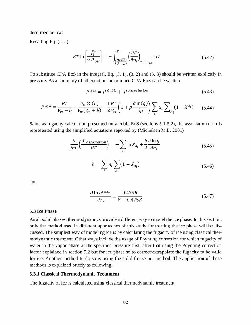
82

described below:

Recalling Eq. (5. 5)

To substitute CPA EoS in the integral, Eq. (3. 1), (3. 2) and (3. 3) should be written explicitly in

pressure. As a summary of all equations mentioned CPA EoS can be written

Same as fugacity calculation presented for a cubic EoS (sections 5.1-5.2), the association term is

represented using the simplified equations reported by (Michelsen M.L. 2001)

and

5.3 Ice Phase

As all solid phases, thermodynamics provide a different way to model the ice phase. In this section,

only the method used in different approaches of this study for treating the ice phase will be dis-

cussed. The simplest way of modeling ice is by calculating the fugacity of ice using classical ther-

modynamic treatment. Other ways include the usage of Poynting correction for which fugacity of

water in the vapor phase at the specified pressure first, after that using the Poynting correction

factor explained in section 5.2 but for ice phase so to correct/extrapolate the fugacity to be valid

for ice. Another method to do so is using the solid freeze-out method. The application of these

methods is explained briefly as following.

5.3.1 Classical Thermodynamic Treatment

The fugacity of ice is calculated using classical thermodynamic treatment

𝑅𝑇 ln [𝑓𝑖

𝑣

𝑦𝑖𝑃𝑙𝑜𝑤] = −∫ (

𝜕𝑃

𝜕𝑛𝑖)

𝑇,𝑃,𝑛𝑗≠𝑖

𝑑𝑉 𝑉

(𝑛𝑇𝑅𝑇𝑃𝑙𝑜𝑤

)

(5.42)

𝑃 𝑠𝑦𝑠 = 𝑃 𝐶𝑢𝑏𝑖𝑐 + 𝑃 𝐴𝑠𝑠𝑜𝑐𝑖𝑎𝑡𝑖𝑜𝑛 (5.43)

𝑃 𝑠𝑦𝑠 =𝑅𝑇

𝑉𝑚 − 𝑏−

𝑎0 ∝ (𝑇)

𝑉𝑚(𝑉𝑚 + 𝑏)−

1

2

𝑅𝑇

𝑉𝑚(1 + 𝜌

𝜕 ln(𝑔)

𝜕𝜌)∑𝑥𝑖

𝑖

∑ (1 − 𝑋𝐴𝑖)𝐴𝑖

(5.44)

𝜕

𝜕𝑛𝑖(𝐴𝑟

𝑎𝑠𝑠𝑜𝑐𝑖𝑎𝑡𝑖𝑜𝑛

𝑅𝑇) = −∑ln𝑋𝐴𝑖

𝐴𝑖

+ℎ

2

𝜕 ln𝑔

𝜕𝑛𝑖 (5.45)

ℎ = ∑𝑛𝑖

𝑖

∑(1 − 𝑋𝐴𝑖)

𝐴𝑖

(5.46)

𝜕 ln 𝑔𝑠𝑖𝑚𝑝.

𝜕𝑛𝑖=

0.475𝐵

𝑉 − 0.475𝐵 (5.47)

83

where

• 𝑓𝑖,𝑜 refers to the property if component i in the ideal gas state.

• 𝑔𝑖,𝑠 is Gibbs energy of component i in a solid phase.

• 𝑔𝑖,𝑜 is Gibbs energy of component i in the ideal gas state

• 𝑔𝑖,𝑠 is given by

However, since there is only one component in the pure solid phase (ice), all other components are

assumed to have an infinite fugacity in the pure phases.

5.3.2 Poynting Correction Method

The fugacity of ice is calculated using the Poynting correction on the same basis that was shown

in section 5.2 via the following equation provided by (HydraFLASH n.d.)

where

• 𝑓𝑤𝐼 is the fugacity of water in the ice phase

• ∅𝑤𝑆𝑎𝑡 is the fugacity coefficient of water in the vapor phase at the specified pressure

• 𝑣𝐼 is the ice molar volume

• 𝑃 is the vapor pressure of ice

in which

𝑓𝑖,𝑠 = 𝑓𝑖,𝑜𝑒𝑥𝑝 [𝑔𝑖,𝑠 − 𝑔𝑖,𝑜

𝑅𝑇] (5.48)

𝑔𝑖,𝑠

𝑅𝑇=

𝑔𝑖0,𝑠

𝑅𝑇0− ∫

ℎ𝑖,𝑠

𝑅𝑇2

𝑇

𝑇0

𝑑𝑇 + ∫𝑉𝑖,𝑠

𝑅𝑇

𝑃

𝑃0

𝑑𝑃 (5.49)

𝑓𝑤𝐼 = ∅𝑤

𝑆𝑎𝑡𝑃𝐼𝑆𝑎𝑡𝑒𝑥𝑝 (

𝑣𝐼(𝑃 − 𝑃𝐼𝑆𝑎𝑡)

𝑅𝑇)𝑃 (5.50)

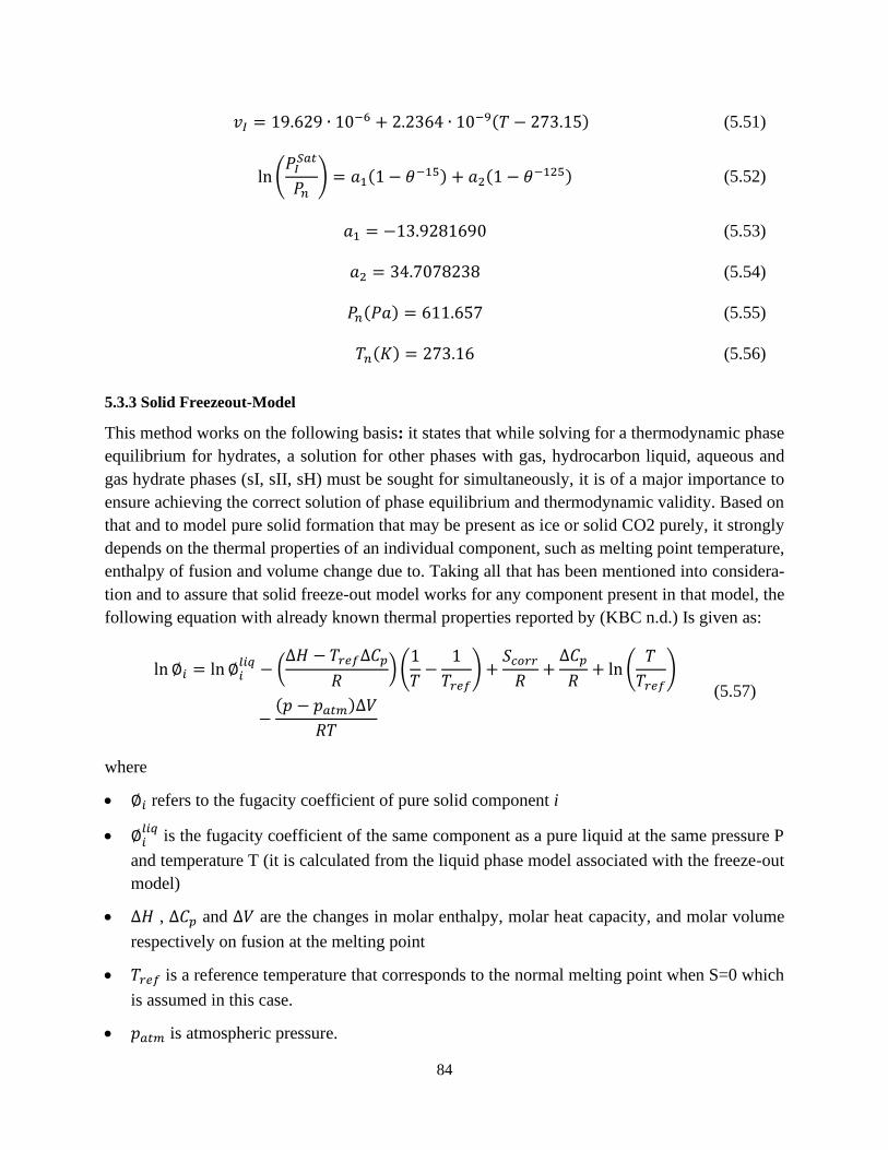
84

5.3.3 Solid Freezeout-Model

This method works on the following basis: it states that while solving for a thermodynamic phase

equilibrium for hydrates, a solution for other phases with gas, hydrocarbon liquid, aqueous and

gas hydrate phases (sI, sII, sH) must be sought for simultaneously, it is of a major importance to

ensure achieving the correct solution of phase equilibrium and thermodynamic validity. Based on

that and to model pure solid formation that may be present as ice or solid CO2 purely, it strongly

depends on the thermal properties of an individual component, such as melting point temperature,

enthalpy of fusion and volume change due to. Taking all that has been mentioned into considera-

tion and to assure that solid freeze-out model works for any component present in that model, the

following equation with already known thermal properties reported by (KBC n.d.) Is given as:

where

• ∅𝑖 refers to the fugacity coefficient of pure solid component i

• ∅𝑖𝑙𝑖𝑞

is the fugacity coefficient of the same component as a pure liquid at the same pressure P

and temperature T (it is calculated from the liquid phase model associated with the freeze-out

model)

• ∆𝐻 , ∆𝐶𝑝 and ∆𝑉 are the changes in molar enthalpy, molar heat capacity, and molar volume

respectively on fusion at the melting point

• 𝑇𝑟𝑒𝑓 is a reference temperature that corresponds to the normal melting point when S=0 which

is assumed in this case.

• 𝑝𝑎𝑡𝑚 is atmospheric pressure.

𝑣𝐼 = 19.629 ∙ 10−6 + 2.2364 ∙ 10−9(𝑇 − 273.15) (5.51)

ln (𝑃𝐼

𝑆𝑎𝑡

𝑃𝑛) = 𝑎1(1 − 𝜃−15) + 𝑎2(1 − 𝜃−125) (5.52)

𝑎1 = −13.9281690 (5.53)

𝑎2 = 34.7078238 (5.54)

𝑃𝑛(𝑃𝑎) = 611.657 (5.55)

𝑇𝑛(𝐾) = 273.16 (5.56)

ln ∅𝑖 = ln∅𝑖𝑙𝑖𝑞 − (

∆𝐻 − 𝑇𝑟𝑒𝑓∆𝐶𝑝

𝑅)(

1

𝑇−

1

𝑇𝑟𝑒𝑓) +

𝑆𝑐𝑜𝑟𝑟

𝑅+

∆𝐶𝑝

𝑅+ ln (

𝑇

𝑇𝑟𝑒𝑓)

−(𝑝 − 𝑝𝑎𝑡𝑚)∆𝑉

𝑅𝑇

(5.57)

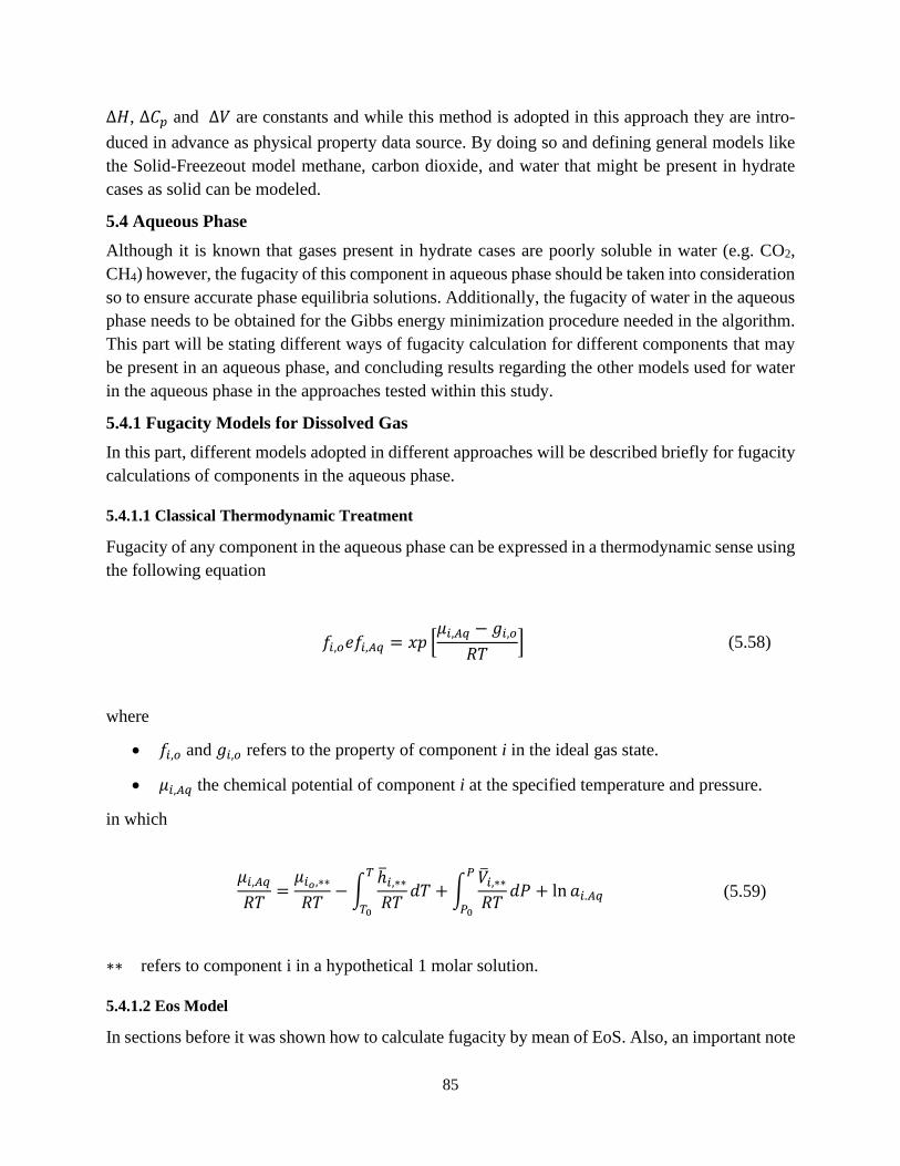
85

∆𝐻, ∆𝐶𝑝 and ∆𝑉 are constants and while this method is adopted in this approach they are intro-

duced in advance as physical property data source. By doing so and defining general models like

the Solid-Freezeout model methane, carbon dioxide, and water that might be present in hydrate

cases as solid can be modeled.

5.4 Aqueous Phase

Although it is known that gases present in hydrate cases are poorly soluble in water (e.g. CO2,

CH4) however, the fugacity of this component in aqueous phase should be taken into consideration

so to ensure accurate phase equilibria solutions. Additionally, the fugacity of water in the aqueous

phase needs to be obtained for the Gibbs energy minimization procedure needed in the algorithm.

This part will be stating different ways of fugacity calculation for different components that may

be present in an aqueous phase, and concluding results regarding the other models used for water

in the aqueous phase in the approaches tested within this study.

5.4.1 Fugacity Models for Dissolved Gas

In this part, different models adopted in different approaches will be described briefly for fugacity

calculations of components in the aqueous phase.

5.4.1.1 Classical Thermodynamic Treatment

Fugacity of any component in the aqueous phase can be expressed in a thermodynamic sense using

the following equation

where

• 𝑓𝑖,𝑜 and 𝑔𝑖,𝑜 refers to the property of component i in the ideal gas state.

• 𝜇𝑖,𝐴𝑞 the chemical potential of component i at the specified temperature and pressure.

in which

∗∗ refers to component i in a hypothetical 1 molar solution.

5.4.1.2 Eos Model

In sections before it was shown how to calculate fugacity by mean of EoS. Also, an important note

𝑓𝑖,𝑜𝑒𝑓𝑖,𝐴𝑞 = 𝑥𝑝 [𝜇𝑖,𝐴𝑞 − 𝑔𝑖,𝑜

𝑅𝑇] (5.58)

𝜇𝑖,𝐴𝑞

𝑅𝑇=

𝜇𝑖𝑜,∗∗

𝑅𝑇− ∫

ℎ̅𝑖,∗∗

𝑅𝑇

𝑇

𝑇0

𝑑𝑇 + ∫�̅�𝑖,∗∗

𝑅𝑇

𝑃

𝑃0

𝑑𝑃 + ln 𝑎𝑖.𝐴𝑞 (5.59)

86

has been written in the text state that in all approaches where EoS model has been used, the algo-

rithm or the calculation always start using a CPA EoS, in which when polar components are en-

countered in any phase, the association term of CPA will be active while it is not in other cases.

Similarly, in an aqueous phase, for dissolved polar components gas (e.g. CO2) , fugacity is calcu-

lated within a complete CPA EoS (association term present ) while for non-polar gas components

(e.g.) the association term is eliminated directly.

5.4.2 Fugacity Models for Water

Following the same procedure, this section describes briefly different models adopted in different

approaches for fugacity calculation of water component in the aqueous phase.

5.4.2.1 Classical Thermodynamic Treatment

Fugacity of water in the aqueous phase can be expressed in a thermodynamic sense similarly to

Eq. (5. 48) as following

where

• 𝑓𝑤𝑜 and 𝑔𝑤0 refers to the property of water in the ideal gas state (1 bar).

• 𝜇𝑤,𝐴𝑞 Is the chemical potential of water at the specified temperature and pressure.

in which

∗∗ refers to the pure liquid water phase.

Keep in mind what was mentioned at the beginning and in different sections of this chapter. The

main objective of this chapter is to make the reader familiar with different models used in different

approaches for all cases except systems where salts and inhibitors are not present. The extension

of this model for the remaining cases will be discussed in other parts of this work. At this stage,

for cases where salts (electrolytes) are present in the system and for cases where the classical

thermodynamic model is used, an additional term is needed, the activity coefficient term.

5.4.2.2 Eos Model

This section is just to clarify for the reader the already described point that by the usage of EoS

𝑓𝑤𝐴𝑞 = 𝑓𝑤𝑜 . 𝑒𝑥𝑝 [

𝜇𝑤,𝐴𝑞 − 𝑔𝑤0

𝑅. 𝑇] (5.60)

𝜇𝑤,𝐴𝑞

𝑅𝑇=

𝑔𝑤𝑜,∗

𝑅𝑇0− ∫

ℎ𝑤,∗

𝑅𝑇2

𝑇

𝑇0

𝑑𝑇 + ∫𝑉𝑤,∗

𝑅𝑇

𝑃

𝑃0

𝑑𝑃 (5.61)

87

models for fugacity calculations, all approaches tested use CPA EoS. Since water is considered a

weekly-polar component in which microscopical hydrogen bonding (self-association) needs to be

described, the association term is always active for water case. Based on that and as water is present

in all the phases (e.g. vapor) fugacity is calculated within CPA EoS. For a full description of the

fugacity model using CPA EoS, refer to section 5.1.

88

Chapter 6

6.1 Approaches Application

The main objective of this study is to provide the oil and gas industry with answers about the

accuracy regarding each method/approach used for hydrate calculations. In addition, choosing an

accurate prediction tool that may serve as an optimization tool is also of vital importance. The

selected approach should be able to predict as accurately as possible hydrate formation at specific

temperature/pressure, at a given overall composition. By providing such a tool, the oil and gas

industry will be able to decrease the daily operation expenditure (OPEX) by decreasing the inhib-

itor cost. An accurate trustful hydrate predicting approach may serve as an optimization tool for

inhibitor volume/cost. This is accomplished by minimizing the required shifting of hydrate for-

mation conditions (P-T) toward higher ones, at which more energy is required in the system to

form hydrate. To achieve that, the used approach/tool must be able to predict accurately the inhi-

bition effect. By attaining this goal, we help in optimizing and identifying the best method needed

to be applied in pipelines to avoid blockage. Such a tool provides necessary information about

different inhibitors scenario (type and concentration) and other methods (e.g. Cold flow) that can

be applied to avoid pipeline blockages. By doing so, the oil and gas industry will be able to com-

pare accurately different methods based on while low financial cost, efficiency, and validity will

be accomplished together for different cases.

Based on that, in this work, we considered the six well-known approaches that have been recom-

mended and reported as of today’s most accurate and state-of-the-art ones for hydrates modeling.

These approaches are implemented in four commercial software packages considered as today’s

best solutions offered in the market for modeling hydrates. However, this study can be considered

as a state-of-art for the hydrate prediction accuracy of the already market’s present programs. A

comparison is provided based on hydrate formation pressure/temperature. All of these methods/ap-

proaches are tested against a large number of experimental hydrate pressure and temperature dis-

sociation data collected from the literature, published between the years of 2015 and 2020. In this

chapter, only data related to systems containing CO2 are discussed and results obtained are ana-

lyzed both quantitatively and qualitatively.

6.2 Background of the Study

The background of this study is mainly related to oil and gas transportation in pipelines. Thus,

accurate predictions of natural gas hydrates formation and inhibition effect is of main interest. To

examine the accuracy and prediction strength of each approach, experimental data are reproduced

within each approach. Within specific methodology, the deviations of each method are examined.

Consequently, analysis and recommendations based on the results obtained are reported. To inves-

tigate the accuracy of different models, present, several factors have been taken into consideration.

The most important factor is the presence of CO2 components in the system and inaccuracy intro-

duced due to its non-ideal behavior.

89

Thus, the CO2 component is a good start to test the strength and accuracy of each approach used.

6.2.1 The Need of an Accurate Model for Co2 Hydrate

Several organizations and environmental committees (e.g. European Projects Association (EPA))

are focusing on reducing CO2 emission from large power plants and major industrial processes by

capturing the CO2 for geological sequestration. Several reports have investigated the potential for

geological sequestration of CO2 and association costs related to the outcome of which is that CO2

storage in Deep Ocean is the likely long-term destination of the large atmospheric releases of CO2

in Europe. Under the conditions prevailing at Deep Ocean (low temperature, high pressure) and

the contact of CO2 with seawater, CO2 hydrates are formed. The necessity and the low cost of CO2

storage in Deep Ocean encouraged different institutes and industries to run dozens of projects on

the application of this method for reducing CO2 concentration in the atmosphere. However, crucial

factors that are considered in the application of this method are the formation and stability of CO2

hydrates in the Deep Ocean. An accurate prediction of these factors requires a capable and accurate

hydrate approach/model. As a result, the outcome of CO2 hydrate modeling in this work can be

adopted as a clustering tool for the accuracy of different approaches studied in. Besides, the rec-

ommended approach can be used directly for studying the above-mentioned factors.

6.3 Theory and Approaches

The approaches used in this study are today’s best methods predicting hydrates dissociation con-

ditions of a given overall composition. These methods may be classified based on similarities or

differences in which several thermodynamic models are used. All of these approaches use the van

der Waals-Platteeuw model together with a Kihara spherical core potential. Most of them imple-

ment VdW-P in an explicit fugacity-based method for calculating gas hydrate equilibrium condi-

tions. Only one out of six approaches studied uses water chemical potential difference between

empty and actual hydrate for computing equilibrium conditions. However, they differ in the ther-

modynamic and EoS models describing the hydrate co-existent phases (e.g. ice, water, etc.). All

that has been mentioned is explained in detail in both chapters 4 & 5. Chapter 4 covers the original

VdW-P model, it is a modification and different way of implying this model for hydrate equilibria

problem. Chapter 5 covers different thermodynamic and EoS models used for the description of

hydrate co-existing phases. In this section, we will review each approach Models used to describe

equilibrium in all phases of a hydrating system.

6.3.1 Approach Nº1: Parrish and Prausnitz (1972) “CSMHyd”

(Prausnitz W 1972) Were the first who presented an algorithm for VdW-P theory to become suit-

able for computer implementation. The first program that adopted and implemented this model is

the CSMHyd program (Sloan ED 2008). Sloan has shown that the P-P model can similarly be

derived by the use of statistical mechanics. However, P-P derived their model by use of a chemical

reaction theory and classical thermodynamic relations basis (Section 4.3). Despite that, CSMHyd

adopted the P-P method in which the main feature used in this study is hydrate temperature or

pressure predictions.

90

The basis of the model present in CSMHyd assumes that within the presence of the four factors,

i.e. water, light hydrocarbon gases, low temperature and high pressure, hydrate is always formed.

In other words, no stability analysis targeting different combinations for phase fractions/composi-

tions that minimize locally or globally Gibbs energy and satisfy material balance is needed. Ac-

cordingly, the predicted hydrate's structure (sI and sII) are based on an already introduced instruc-

tion to the algorithm. For example, CO2 pure hydrate always and only forms an sI structure. On

the other hand, the model/program identifies the formation of hydrate within the ice/water co-

existing phase based on a reference temperature of 273.15 K which denotes the triple point of

water. Accordingly, if T<273.15 the model assumes ice presence whereas water is assumed if it is

equal or higher. Similarly, the model identifies the vapor or condensed gas region (different locus

of P-T diagram) based on quadruple experimental data points collected from the literature for dif-

ferent gases. Regarding CO2 the upper quadruple point conditions for hydrate of pure CO2 gas are

283.5 K and 4.537110 MPa. The model adopts these values and will check for the T of the system.

If T<283.5 it assumes that pure CO2 hydrates form in the region of hydrate-water-vapor region. If

not, hydrates will form in the water-condensed gas region at higher pressure.

On the other hand, the chemical potential difference between empty and actual hydrate is used for

the calculation of equilibrium conditions. It aims at the basis that chemical potential is a state

function and by equalizing theoretical to experimental difference and iterating for the pressure,

dissociation/formation pressure of hydrates is calculated. A typical Newton-Raphson technique is

used for this purpose. For full detail of the algorithm and steps followed review section 4.3. Finally,

the Soave-Redlich-Kwong equation is used to model hydrocarbon phases in the model. However,

the fugacity of water and gas dissolved in the aqueous phase are treated using fundamental ther-

modynamic relationships explained in section 5.4 of this work.

6.3.2 Approach Nº2: Ballard and Sloan (2002) “CSMGem”

After the adoption of the Parrish and Prausnitz method in CSMHyd software developed by E.

Sloan, the main improvements on the hydrate phase equilibria problem occurred. It made it provide

a faster and safer prediction of the hydrate equilibrium conditions. The new method allows direct

calculation of water fugacity in hydrate instead of equalizing the chemical potential difference.

Moreover, it provides a faster convergence to the solution by eliminating the second iteration re-

quired by the P-P method. While that improvement happened, Ballard was running spectroscopic

experiments for his Ph.D. under the supervision of Prof. Sloan. During the evaluation of the spec-

troscopic data obtained, they realized significant deviations between VdW predicted values and

the experimental data obtained. Based on that, they proposed modifications to the original hydrate

theory of VdW-P. The main modification aims at adding an activity coefficient to the original

theory to account for the distortion of the lattice structure by guest molecules. The second modifi-

cation provided an easier way for the calculation of water fugacity in hydrates that made it easy to

describe in a thermodynamic sense. On the other hand, several two-phase stability and phase split

tests/approaches were extended to include multiphase systems, such as Gupta’s and Michelsen's

approaches. After all these improvements that may provide more accurate and reliable results,

91

Sloan’s added these auxiliary tools for approach N#1 adopted in CSMHyd. He came up with a

new approach (N#2) and implemented it in another software “CSMGem”, an acronym for Colo-

rado School of Mines (Gibbs energy minimization).

This approach (Approach N#2) utilizes the same models already used in Approach N#1 (CSMHyd)

for describing different hydrate co-existence phase. It also uses Soave-Redlich-Kwong (SRK) EoS

for modeling different hydrocarbon phase but also treats gas dissolved and water in the aqueous

phase using classical thermodynamic relationships (Section 5.4). The two modifications of Ballard

to the original VdW-P hydrates model are explained in Chapter 4. Also, Gupta’s stability analysis

for phase existence/absence implemented in this approach is explained in Chapter 2. It is good to

mention here that to initialize or to start the algorithm described in Chapter 2 by mean of Ki’s,

Sloan has reported/used two sets of Ki’s. Both sets can be used as an initial guess. The first set is

generated using composition independent correlation “ideal set Ki’s” while the second one is based

on incipient solid phases. CSMGem gives the choice to identify one of these sets to start calcula-

tions. Although Ki’s don’t play an important role in the solution and are just used as an initial

guess for the algorithm, in this work we choose the ideal set of Ki’s to start our calculation. The

reason for that is to ensure that both methods/approaches (N’1 & 2) do have the same basis in the

computation procedure. Since no data is available about the initial guess used in CSMHyd (N#1)

approach and by taking into consideration the year of implementing Parrish and Prausnitz method

into CSMHyd program (1998) were few experimental data on solid phases was available, we have

assumed that Sloan’s has been using the same ideal Ki’s in his previous approach (N”1).

It is also important to mention that based on the fact that Gupta’s stability method is present in this

approach, no more quadruples data point entry is needed in the algorithm. The outcome of Gupta’s

stability method visualizes the presence or the absence of each phase assumed (Chapter 2). In other

words, the presence of a vapor or condensed gas phase is based on the outcome of Gupta’s stability

parameter. However, the same idea is applicable for the aqueous phase, where it is not anymore

defined by a temperature condition but also depends on Gupta’s test outcome parameter.

6.3.3 Approach Nº3: KBC/MultiFlash RKSA “MF RKSA”

MultiFlash/KBC RKSA's first two words refer to industrial names of the software (MultiFlash)

and the company name providing this approach (KBC). RKSA is an acronym in which the first

three letters refer to SRK/RKS EoS used in the model and letter A to the advancement made. All

together form Redlich-Kwong-Soave-Advanced. However, the major improvement in this

model/approach is the presence of an improved NRTL (Non-Random-Two-Liquids) equation.

This allows the complex behavior of the liquid phase to be represented, whilst maintaining the

good performance of cubic EoS for hydrocarbon phases.

In this work, we will be referring to the approach (N#3) by the abbreviation “MF RKSA”. In this

model, the calculation of hydrates phase equilibria is based on the improved Parrish and Prausnitz

method. Through an “improved” explicit fugacity-based method for calculating gas hydrate equi-

librium conditions is denoted. It becomes clear now, that the solved equation is the equality of

component’s fugacity in all phases present at equilibrium. As it is the case in CSMGem and the

92

presence of Gupta’s application that ensures the stability of phases at equilibrium, the Michelsen

multiphase stability test is used in this MF RKSA. Both methods are used for checking the stability

of possibly existing phases. However, the procedure followed in each one varies. In MF RKSA,

Michelsen’s stability main objective aims at finding phase compositions at which the Tangent Plan

Distance (TPD) is negative. However, material balance is respected in the test by definition (by

assuming an infinitesimal quantity of the trial phase). Based on that, the phase presence is identi-

fied by the Michelsen test where no preliminary conditions are used.

On the other hand, gas and liquid hydrocarbons phases are modeled with the SRK EoS model.

However, the fugacity of liquid hydrocarbon is described by the generalized equation explained in

section 5.2. The first term in the equation is the activity coefficient. As it is explained in section

5.3 it accounts for Excess Gibbs energy. While explaining Eq.5. 29 in Chapter 5, the case has been

considered is that only the EoS equation is used for the description of the liquid phase. Due to that,

the activity coefficient has been neglected. However, in this approach, both the EoS and activity

coefficient is used to represent the liquid phase. In other words, the activity coefficient is activated

for any liquid phase present in the system. In general, the activity coefficient is used to model

liquid phases containing any combination of polar and non-polar components exhibiting a very

strong non-ideality. However, it can be obtained using various equations such as Wilson,

UNIQUAC or NRTL. In this approach (MF RKSA), the NRTL equation is adopted for this pur-

pose. NRTL discussion is not present in this work since it is out of the scope, for more details refer

to any thermodynamic textbook. Additionally, other factors in Eq.5. 29 account for the correction

of fugacity through Poynting correction. All terms present Eq.5. 29 exception of the activity term

can be combined to form Eq. 5. 30. This equation is just a combination of the fugacity coefficient

of components obtained from SRK EoS and the saturation pressure of the component. Adding to

that, the Poynting correction term is present.

Apart from the gas and liquid phases, the aqueous phase is also calculated using Eq.5. 2 in the

same way, described before. In general, the activity coefficient will be always activated for the

aqueous phase.

However, no big effect is observed in the results when pure water is present. This term becomes

important when CO2 is dissolved in water.

The only remaining phase that needs to be modeled is the solid phase. Utilizing solid phase, solid

CO2 and ice are referred. To represent the solid phase, MF-RKSA uses the Solid Freeze-Out model

described in 5.3.3.

6.3.4 Approach N#4: KBC/MultiFlash CPA “MF CPA”

Due to the difficulties present in modeling the aqueous phase, particularly if inhibitors and/or salts

are present, MultiFlash software provides an alternative model/tool for modeling hydrates. How-

ever, KBC/MultiFlash Company recommends the use of this model/approach for systems includ-

ing inhibitors. This approach is based on the CPA EoS to represent all phases present in a hydrated

93

system. Based on that, the CPA EoS represents each phase having both non-association and asso-

ciation terms. Dealing with vapor hydrocarbons, the non-association term is always present and

represented by the SRK cubic term. On the other hand, the association term is only activated when

polar components such as CO2 exists in the gas phase. CPA also covers the liquid hydrocarbon

phase in the same way. For an aqueous phase and for both cases of water with/without dissolved

gas (e.g. CO2 or methane), both terms of the CPA are always present. The reason is that water is a

polar compound, thus hydrogen bonding needs to be represented within the second term. For a

solid phase, this approach adopts the Solid Freezeout model presented in section 5.3.3. The basis

of which different energy terms should be included. Finally, MultiFlash software adopts Michel-

sen’s test for phase stability in different hydrate approaches supported.

6.3.5 Approach Nº5&6: HydraFLASH/HydraFact CPA, Both Approaches “HF” & “HF72”

Hydra Flash/Hydra Fact is the names of the software and the developing company providing it

respectively. In this software, a CPA-EoS based model is used to perform hydrate calculations.

However, due to the difficulties in representing hydrate-co existence phases, HydraFLASH soft-

ware gives the user the choice to select the cubic part of the CPA EoS. Based on that two non-

association-cubic EoS are used to describe each system of this work. The first chosen EoS is

Soave-Redlich-Kwong while the second one is SRK72. Since both approaches are CPA based ones

with differences in the association term, they are labeled as HF & HF72. In both approaches, the

CPA EoS covers all phases present in a hydrated system. However, the association term is acti-

vated only when polar components are encountered in some phases. On the other hand, in both

approaches, HF & HF72, the solid phase fugacity is corrected using the Poynting method described

in 5.3.2. Finally, the already described Michelsen’s multiphase test is used to ensure the stability

of all phases in equilibrium.

6.4 Experimental Work

6.4.1 Methodology

All experimental data are available in the literature that was published after 2015 and were re-

trieved and organized according to their content (i.e. CO2 mixtures, salts, inhibitors, etc.). In this

Chapter, only data related to systems containing CO2 are discussed. Subsequently, all data were

introduced to the software available, namely Hydra Flash (Hydra Fact), MultiFlash (KBC),

CSMGem (Colorado School of Mines) and CSMHyd (also Colorado School of Mines). All exper-

imental data related to CO2 mixtures were reproduced using different approaches/models present

in every software:

· HydraFlash with SRK non-associating term (HF).

· HydraFlash with SRK72 non-associating term (HF72).

· Multiphase Flash with CPA model (CPA).

· Multiphase Flash with RKSA model (RKSA).

· CSMGem.

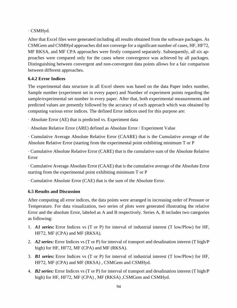
94

· CSMHyd.

After that Excel files were generated including all results obtained from the software packages. As

CSMGem and CSMHyd approaches did not converge for a significant number of cases, HF, HF72,

MF RKSA, and MF CPA approaches were firstly compared separately. Subsequently, all six ap-

proaches were compared only for the cases where convergence was achieved by all packages.

Distinguishing between convergent and non-convergent data points allows for a fair comparison

between different approaches.

6.4.2 Error Indices

The experimental data structure in all Excel sheets was based on the data Paper index number,

Sample number (experiment set in every paper) and Number of experiment points regarding the

sample/experimental set number in every paper. After that, both experimental measurements and

predicted values are presently followed by the accuracy of each approach which was obtained by

computing various error indices. The defined Error indices used for this purpose are:

· Absolute Error (AE) that is predicted vs. Experiment data

· Absolute Relative Error (ARE) defined as Absolute Error / Experiment Value

· Cumulative Average Absolute Relative Error (CAARE) that is the Cumulative average of the

Absolute Relative Error (starting from the experimental point exhibiting minimum T or P

· Cumulative Absolute Relative Error (CARE) that is the cumulative sum of the Absolute Relative

Error

· Cumulative Average Absolute Error (CAAE) that is the cumulative average of the Absolute Error

starting from the experimental point exhibiting minimum T or P

· Cumulative Absolute Error (CAE) that is the sum of the Absolute Error.

6.5 Results and Discussion

After computing all error indices, the data points were arranged in increasing order of Pressure or

Temperature. For data visualization, two series of plots were generated illustrating the relative

Error and the absolute Error, labeled as A and B respectively. Series A, B includes two categories

as following:

1. A1 series: Error Indices vs (T or P) for interval of industrial interest (T low/Plow) for HF,

HF72, MF (CPA) and MF (RKSA).

2. A2 series: Error Indices vs (T or P) for interval of transport and desalination interest (T high/P

high) for HF, HF72, MF (CPA) and MF (RKSA).

3. B1 series: Error Indices vs (T or P) for interval of industrial interest (T low/Plow) for HF,

HF72, MF (CPA) and MF (RKSA) , CSMGem and CSMHyd.

4. B2 series: Error Indices vs (T or P) for interval of transport and desalination interest (T high/P

high) for HF, HF72, MF (CPA) , MF (RKSA) ,CSMGem and CSMHyd.

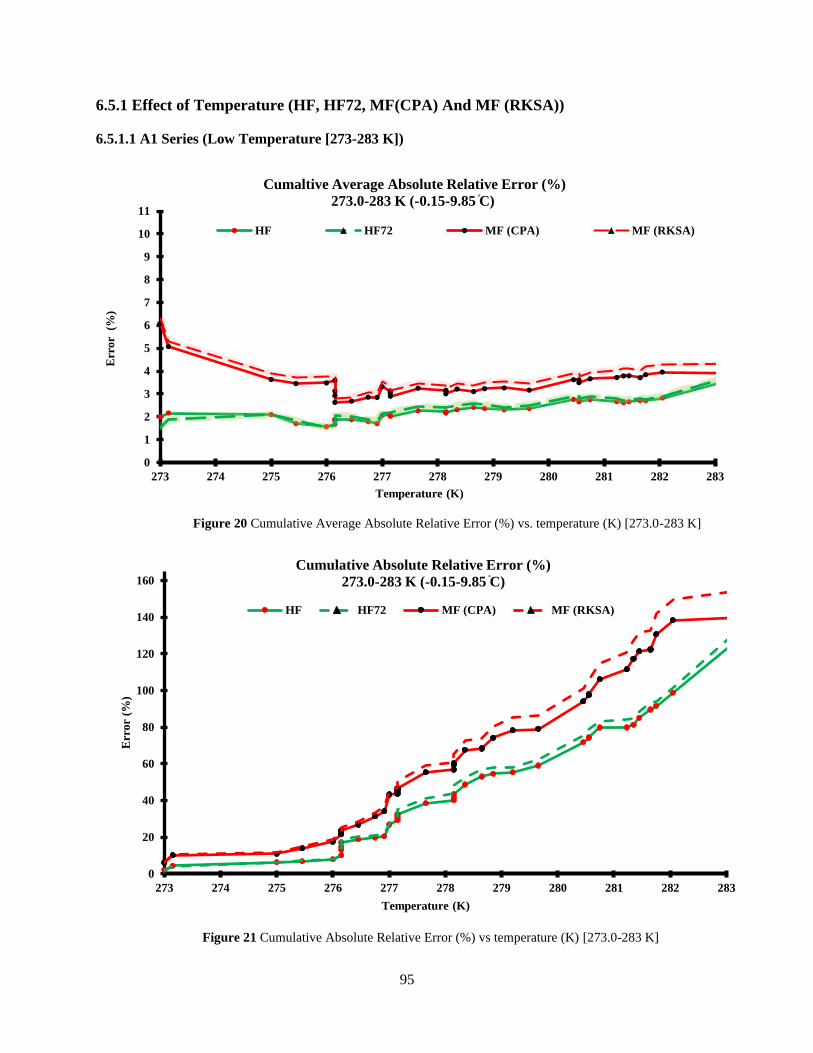
95

6.5.1 Effect of Temperature (HF, HF72, MF(CPA) And MF (RKSA))

6.5.1.1 A1 Series (Low Temperature [273-283 K])

Figure 20 Cumulative Average Absolute Relative Error (%) vs. temperature (K) [273.0-283 K]

Figure 21 Cumulative Absolute Relative Error (%) vs temperature (K) [273.0-283 K]

0

1

2

3

4

5

6

7

8

9

10

11

273 274 275 276 277 278 279 280 281 282 283

Err

or

(%

)

Temperature (K)

Cumaltive Average Absolute Relative Error (%)

273.0-283 K (-0.15-9.85 ֯C)

HF HF72 MF (CPA) MF (RKSA)

0

20

40

60

80

100

120

140

160

273 274 275 276 277 278 279 280 281 282 283

Err

or

(%)

Temperature (K)

Cumulative Absolute Relative Error (%)

273.0-283 K (-0.15-9.85 ֯C)

HF HF72 MF (CPA) MF (RKSA)

96

Figure 22 Cumulative Average Absolute Error (MPa) vs. temperature (K) [273.0-283 K]

Figure 23 Cumulative Absolute Error (MPa) vs temperature (K) [273-283 K]

Figures 20, 21, 22 and 23 show different error indices for low temperature range (273-283 K).

Examining the results obtained for low-temperature range (273-283 K) present in series of figures

,a clear difference in the accuracy/deviation between MultiFlash and HydraFlash approaches

adopted is noticed. Also, it is quite clear that approaches adopted by each software show more or

less the same deviation at low temperatures. While reproducing the data related to this part (low

0.00

0.05

0.10

0.15

0.20

0.25

273 274 275 276 277 278 279 280 281 282 283

Err

or

(Mp

a)

Temperature (K)

Cumulative Average Absolute error (MPa)

273.0-283 K (-0.15-9.85 ֯C)

HF HF72 MF (CPA) MF (RKSA)

0.00

1.00

2.00

3.00

4.00

5.00

6.00

273 275 277 279 281 283

Err

or

(Mp

a)

Temperature (K)

Cumulative Absolute error (MPa)

273.0-283 K (-0.15-9.85 ֯C)

HF HF72 MF (CPA) MF (RKSA)

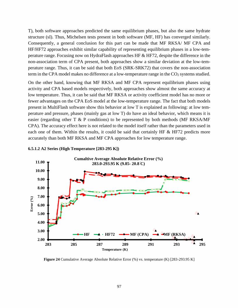
97

T), both software approaches predicted the same equilibrium phases, but also the same hydrate

structure (sI). Thus, Michelsen tests present in both software (MF, HF) has converged similarly.

Consequently, a general conclusion for this part can be made that MF RKSA/ MF CPA and

HF/HF72 approaches exhibit similar capability of representing equilibrium phases in a low-tem-

perature range. Focusing now on HydraFlash approaches HF & HF72, despite the difference in the

non-association term of CPA present, both approaches show a similar deviation at the low-tem-

perature range. Thus, it can be said that both EoS (SRK-SRK72) that covers the non-association

term in the CPA model makes no difference at a low-temperature range in the CO2 systems studied.

On the other hand, knowing that MF RKSA and MF CPA represent equilibrium phases using

activity and CPA based models respectively, both approaches show almost the same accuracy at

low temperature. Thus, it can be said that MF RKSA or activity coefficient model has no more or

fewer advantages on the CPA EoS model at the low-temperature range. The fact that both models

present in MultiFlash software show this behavior at low T is explained as following: at low tem-

perature and pressure, phases (mainly gas at low T) do have an ideal behavior, which means it is

easier (regarding other T & P conditions) to be represented by both methods (MF RKSA/MF

CPA). The accuracy effect here is not related to the model itself rather than the parameters used in

each one of them. Within the results, it could be said that certainly HF & HF72 predicts more

accurately than both MF RKSA and MF CPA approaches for low temperature range.

6.5.1.2 A2 Series (High Temperature [283-295 K])

Figure 24 Cumulative Average Absolute Relative Error (%) vs. temperature (K) [283-293.95 K]

2.00

3.00

4.00

5.00

6.00

7.00

8.00

9.00

10.00

11.00

283 285 287 289 291 293 295

Err

or

(%)

Temperature (K)

Cumaltive Average Absolute Relative Error (%)

283.0-293.95 K (9.85- 20.8 ֯C)

HF HF72 MF (CPA) MF (RKSA)

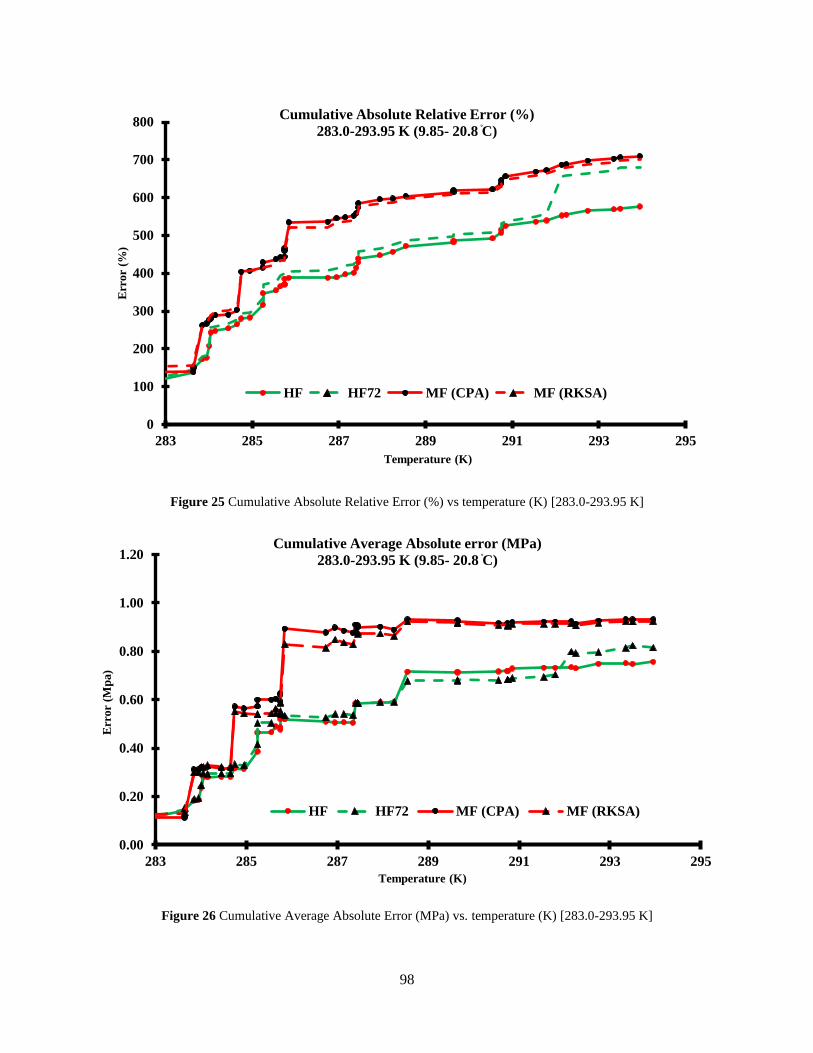
98

Figure 25 Cumulative Absolute Relative Error (%) vs temperature (K) [283.0-293.95 K]

Figure 26 Cumulative Average Absolute Error (MPa) vs. temperature (K) [283.0-293.95 K]

0

100

200

300

400

500

600

700

800

283 285 287 289 291 293 295

Err

or

(%)

Temperature (K)

Cumulative Absolute Relative Error (%)

283.0-293.95 K (9.85- 20.8 ֯C)

HF HF72 MF (CPA) MF (RKSA)

0.00

0.20

0.40

0.60

0.80

1.00

1.20

283 285 287 289 291 293 295

Err

or

(Mp

a)

Temperature (K)

Cumulative Average Absolute error (MPa)

283.0-293.95 K (9.85- 20.8 ֯C)

HF HF72 MF (CPA) MF (RKSA)

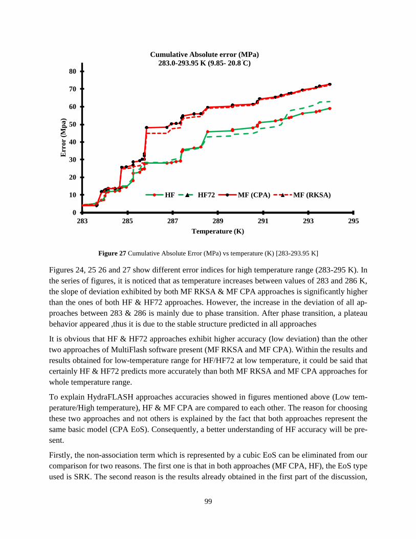
99

Figure 27 Cumulative Absolute Error (MPa) vs temperature (K) [283-293.95 K]

Figures 24, 25 26 and 27 show different error indices for high temperature range (283-295 K). In

the series of figures, it is noticed that as temperature increases between values of 283 and 286 K,

the slope of deviation exhibited by both MF RKSA & MF CPA approaches is significantly higher

than the ones of both HF & HF72 approaches. However, the increase in the deviation of all ap-

proaches between 283 & 286 is mainly due to phase transition. After phase transition, a plateau

behavior appeared ,thus it is due to the stable structure predicted in all approaches

It is obvious that HF & HF72 approaches exhibit higher accuracy (low deviation) than the other

two approaches of MultiFlash software present (MF RKSA and MF CPA). Within the results and

results obtained for low-temperature range for HF/HF72 at low temperature, it could be said that

certainly HF & HF72 predicts more accurately than both MF RKSA and MF CPA approaches for

whole temperature range.

To explain HydraFLASH approaches accuracies showed in figures mentioned above (Low tem-

perature/High temperature), HF & MF CPA are compared to each other. The reason for choosing

these two approaches and not others is explained by the fact that both approaches represent the

same basic model (CPA EoS). Consequently, a better understanding of HF accuracy will be pre-

sent.

Firstly, the non-association term which is represented by a cubic EoS can be eliminated from our

comparison for two reasons. The first one is that in both approaches (MF CPA, HF), the EoS type

used is SRK. The second reason is the results already obtained in the first part of the discussion,

0

10

20

30

40

50

60

70

80

283 285 287 289 291 293 295

Err

or

(Mp

a)

Temperature (K)

Cumulative Absolute error (MPa)

283.0-293.95 K (9.85- 20.8 ֯C)

HF HF72 MF (CPA) MF (RKSA)

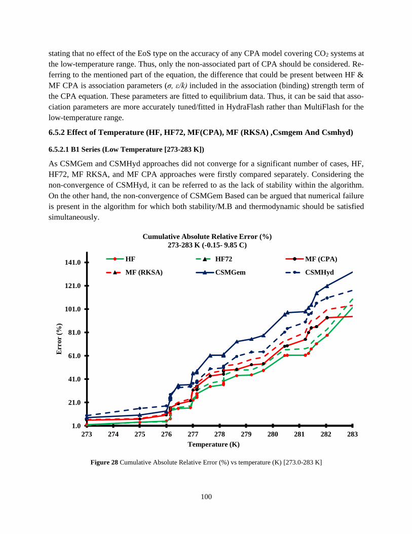
100

stating that no effect of the EoS type on the accuracy of any CPA model covering CO2 systems at

the low-temperature range. Thus, only the non-associated part of CPA should be considered. Re-

ferring to the mentioned part of the equation, the difference that could be present between HF &

MF CPA is association parameters (σ, ε/k) included in the association (binding) strength term of

the CPA equation. These parameters are fitted to equilibrium data. Thus, it can be said that asso-

ciation parameters are more accurately tuned/fitted in HydraFlash rather than MultiFlash for the

low-temperature range.

6.5.2 Effect of Temperature (HF, HF72, MF(CPA), MF (RKSA) ,Csmgem And Csmhyd)

6.5.2.1 B1 Series (Low Temperature [273-283 K])

As CSMGem and CSMHyd approaches did not converge for a significant number of cases, HF,

HF72, MF RKSA, and MF CPA approaches were firstly compared separately. Considering the

non-convergence of CSMHyd, it can be referred to as the lack of stability within the algorithm.

On the other hand, the non-convergence of CSMGem Based can be argued that numerical failure

is present in the algorithm for which both stability/M.B and thermodynamic should be satisfied

simultaneously.

Figure 28 Cumulative Absolute Relative Error (%) vs temperature (K) [273.0-283 K]

1.0

21.0

41.0

61.0

81.0

101.0

121.0

141.0

273 274 275 276 277 278 279 280 281 282 283

Err

or

(%)

Temperature (K)

Cumulative Absolute Relative Error (%)

273-283 K (-0.15- 9.85 C)

HF HF72 MF (CPA)

MF (RKSA) CSMGem CSMHyd

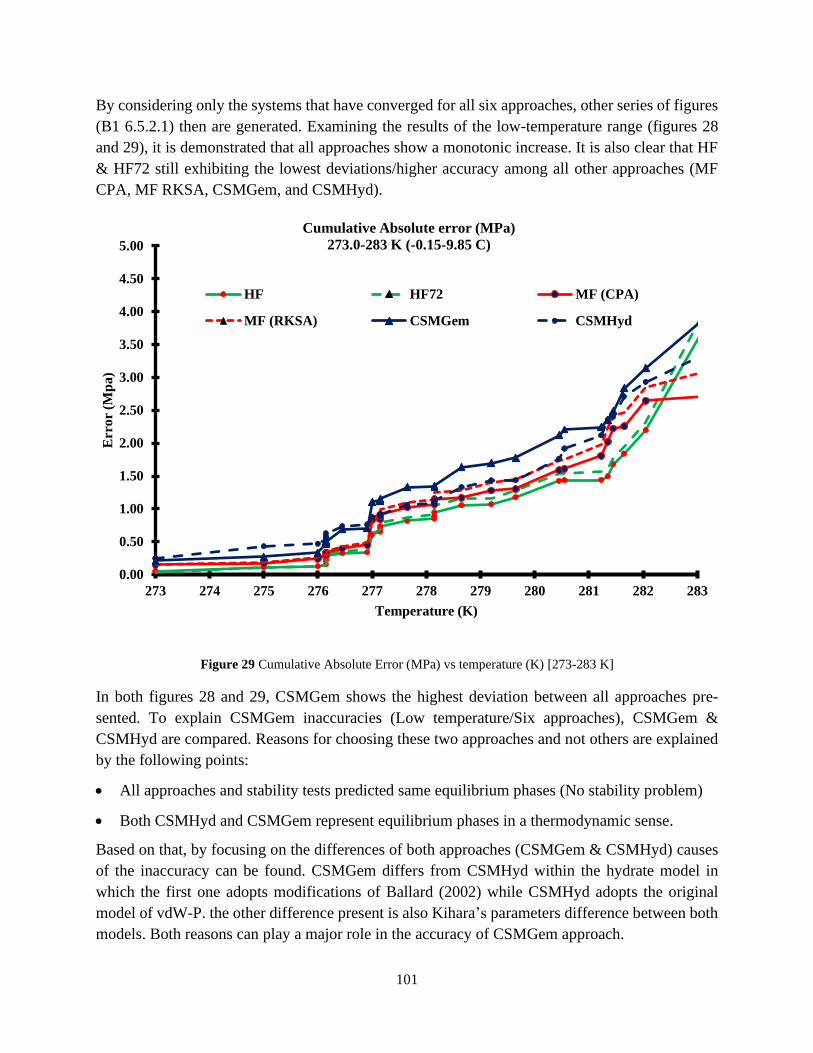
101

By considering only the systems that have converged for all six approaches, other series of figures

(B1 6.5.2.1) then are generated. Examining the results of the low-temperature range (figures 28

and 29), it is demonstrated that all approaches show a monotonic increase. It is also clear that HF

& HF72 still exhibiting the lowest deviations/higher accuracy among all other approaches (MF

CPA, MF RKSA, CSMGem, and CSMHyd).

Figure 29 Cumulative Absolute Error (MPa) vs temperature (K) [273-283 K]

In both figures 28 and 29, CSMGem shows the highest deviation between all approaches pre-

sented. To explain CSMGem inaccuracies (Low temperature/Six approaches), CSMGem &

CSMHyd are compared. Reasons for choosing these two approaches and not others are explained

by the following points:

• All approaches and stability tests predicted same equilibrium phases (No stability problem)

• Both CSMHyd and CSMGem represent equilibrium phases in a thermodynamic sense.

Based on that, by focusing on the differences of both approaches (CSMGem & CSMHyd) causes

of the inaccuracy can be found. CSMGem differs from CSMHyd within the hydrate model in

which the first one adopts modifications of Ballard (2002) while CSMHyd adopts the original

model of vdW-P. the other difference present is also Kihara’s parameters difference between both

models. Both reasons can play a major role in the accuracy of CSMGem approach.

0.00

0.50

1.00

1.50

2.00

2.50

3.00

3.50

4.00

4.50

5.00

273 274 275 276 277 278 279 280 281 282 283

Err

or

(Mp

a)

Temperature (K)

Cumulative Absolute error (MPa)

273.0-283 K (-0.15-9.85 C)

HF HF72 MF (CPA)

MF (RKSA) CSMGem CSMHyd

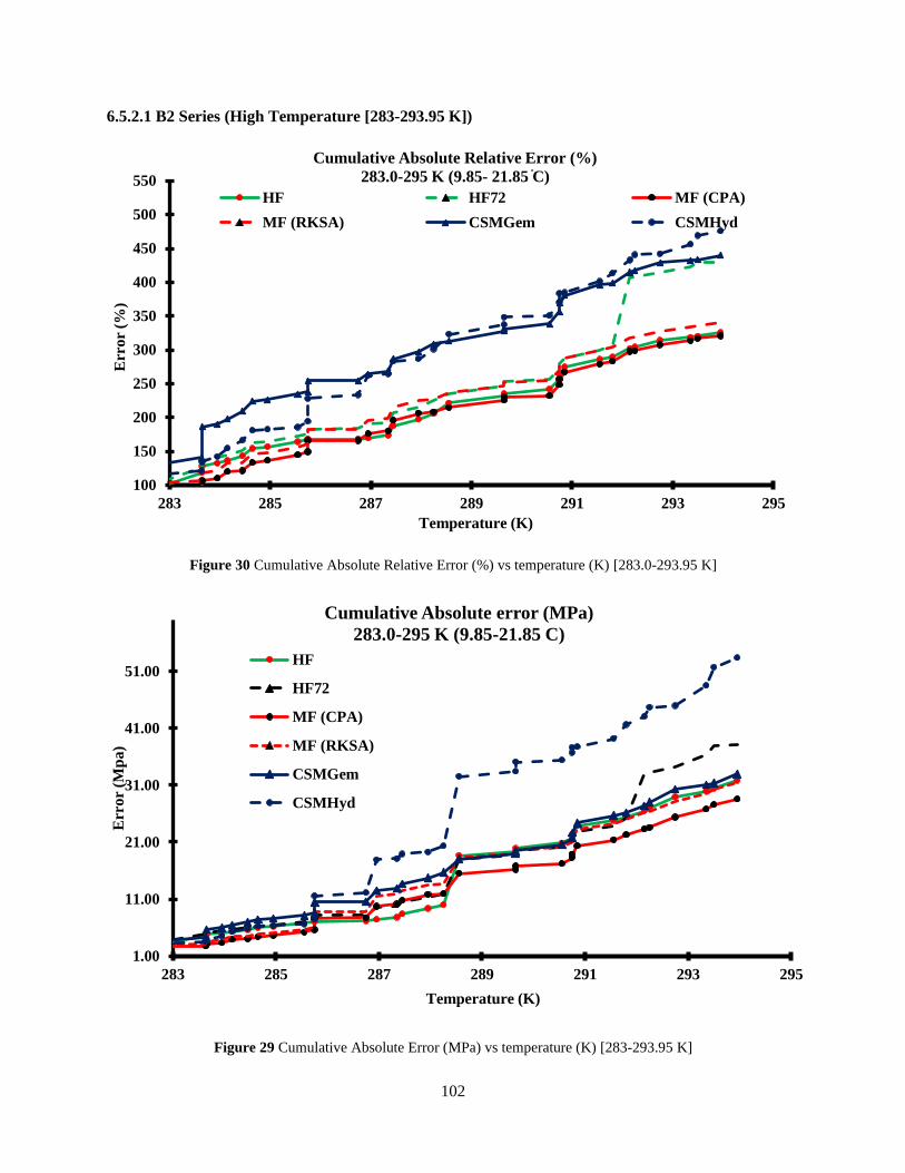
102

6.5.2.1 B2 Series (High Temperature [283-293.95 K])

Figure 30 Cumulative Absolute Relative Error (%) vs temperature (K) [283.0-293.95 K]

Figure 29 Cumulative Absolute Error (MPa) vs temperature (K) [283-293.95 K]

100

150

200

250

300

350

400

450

500

550

283 285 287 289 291 293 295

Err

or

(%)

Temperature (K)

Cumulative Absolute Relative Error (%)

283.0-295 K (9.85- 21.85 ֯C)

HF HF72 MF (CPA)

MF (RKSA) CSMGem CSMHyd

1.00

11.00

21.00

31.00

41.00

51.00

283 285 287 289 291 293 295

Err

or

(Mp

a)

Temperature (K)

Cumulative Absolute error (MPa)

283.0-295 K (9.85-21.85 C)

HF

HF72

MF (CPA)

MF (RKSA)

CSMGem

CSMHyd

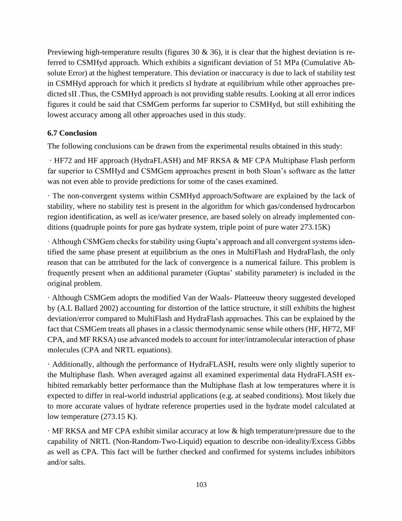
103

Previewing high-temperature results (figures 30 & 36), it is clear that the highest deviation is re-

ferred to CSMHyd approach. Which exhibits a significant deviation of 51 MPa (Cumulative Ab-

solute Error) at the highest temperature. This deviation or inaccuracy is due to lack of stability test

in CSMHyd approach for which it predicts sI hydrate at equilibrium while other approaches pre-

dicted sII .Thus, the CSMHyd approach is not providing stable results. Looking at all error indices

figures it could be said that CSMGem performs far superior to CSMHyd, but still exhibiting the

lowest accuracy among all other approaches used in this study.

6.7 Conclusion

The following conclusions can be drawn from the experimental results obtained in this study:

· HF72 and HF approach (HydraFLASH) and MF RKSA & MF CPA Multiphase Flash perform

far superior to CSMHyd and CSMGem approaches present in both Sloan’s software as the latter

was not even able to provide predictions for some of the cases examined.

· The non-convergent systems within CSMHyd approach/Software are explained by the lack of

stability, where no stability test is present in the algorithm for which gas/condensed hydrocarbon

region identification, as well as ice/water presence, are based solely on already implemented con-

ditions (quadruple points for pure gas hydrate system, triple point of pure water 273.15K)

· Although CSMGem checks for stability using Gupta’s approach and all convergent systems iden-

tified the same phase present at equilibrium as the ones in MultiFlash and HydraFlash, the only

reason that can be attributed for the lack of convergence is a numerical failure. This problem is

frequently present when an additional parameter (Guptas’ stability parameter) is included in the

original problem.

· Although CSMGem adopts the modified Van der Waals- Platteeuw theory suggested developed

by (A.L Ballard 2002) accounting for distortion of the lattice structure, it still exhibits the highest

deviation/error compared to MultiFlash and HydraFlash approaches. This can be explained by the

fact that CSMGem treats all phases in a classic thermodynamic sense while others (HF, HF72, MF

CPA, and MF RKSA) use advanced models to account for inter/intramolecular interaction of phase

molecules (CPA and NRTL equations).

· Additionally, although the performance of HydraFLASH, results were only slightly superior to

the Multiphase flash. When averaged against all examined experimental data HydraFLASH ex-

hibited remarkably better performance than the Multiphase flash at low temperatures where it is

expected to differ in real-world industrial applications (e.g. at seabed conditions). Most likely due

to more accurate values of hydrate reference properties used in the hydrate model calculated at

low temperature (273.15 K).

· MF RKSA and MF CPA exhibit similar accuracy at low & high temperature/pressure due to the

capability of NRTL (Non-Random-Two-Liquid) equation to describe non-ideality/Excess Gibbs

as well as CPA. This fact will be further checked and confirmed for systems includes inhibitors

and/or salts.

104

· HF & HF72 exhibit similar behavior/accuracy as association part in the CPA equation of state

which explains a no effect of Cubic EoS type for the system of CO2 at low and high temperature.

· Finally, based on the outcome of this study, we recommend the usage of HF or HF72 approaches

for hydrate predictions and phase equilibria modeling.

105

References

A.LBallard, E.DSloan Jr. "The next generation of hydrate prediction: I. Hydrate standard states

and incorporation of spectroscopy." Fluid Phase Equilibria, 2002: 371-383.

Andersson V, GudmundssonJ. "Flow properties of hydrate-in-water slurries ." ( N. Y.Acad. Sci)

2000.

Baker, L.E., Pierce, A.C., and Luks, K.D. "Gibbs energy analysis of phase equilibria. ." Soc. Petr.

Eng., (1982): 731-742.

Chapman W.G., Gubbins K.E., Jackson G., Radosz M., ,. "New reference equation of state for

associating liquids." Ind. Eng. Chem., (1990): 1709-1721.

Derawi S.O. Modelling of phase equilibria containing associating fluids. Phd, Denmark: DTU,

2002.

EG, Hammerschmidt. "Formation of gas hydrates in natural gas transmission lines." (Ind. Eng.

Chem.) 26 (1934.).

Florusse LJ, Peters CJ, Schoonman J, Hester KC, Koh CA, Dec SF, Marsh KN, Sloan ED. " Stable

low-pressure hydro¬gen clusters stored in a binary clathrate hydrate. Science. 2004;306:469. ."

n.d.

Fu Y-H., Sandler S.I. "A simplified SAFT equation of state for associating compounds and

mixtures." Ind. Eng. Chem 34 ((1995)): 1897-1909.

Georgios M. Kontogeorgis, Michael L. Michelsen, Georgios K. Folas, Samer Derawi ,Nicolas von

Solms ,Erling H. Stenby. "Ten Years with the CPA (Cubic-Plus-Association) Equation of State.

Part 1. Pure Compounds and Self-Associating Systems." Ind. Eng. Chem. Res, 2006: 4855-4868.

Gibbs, J.W. "On the equilibrium of heterogeneous substances." Vol. I, Dover Publications,

(Reprinted in The Scientific Papers of J. Willard Gibb 1961), 1861.

Gudmundsson JS, Borrehaug A. "Frozen hydrate for transport of natural gas." Toulouse, France:

In Proc. Second Inter-national Conference on Gas Hydrates, June 2-6.1996.

GudmundssonJS, Andersson V, Levik O,MorkM. (. N. Y.Acad. Sci.) 912:403-10 (2000).

GudmundssonJS, Mork M, Graff OF. " Hydrate non-pipeline technology." (Proc. Intl. Conf. Gas

Hydrates 4th) 997-1102. (2002).

Gupta. Steady state simulation of chemical processes. . Phd Thesis, Calgary: University of

Calgary, 1990.

H., Davy. "The Bakerian Lecture. on some of the combinations of oxymuriatic gas and oxygene ,

and on the chemical relations of these principales to inflammable bodies." (Pblios.Trans.R.Soc)

101 (1811): 1:35.

Holder, G. D., Zetts, S. P. and Pradhan, N.,. "Phase Behavior in Systems Containing Clathrate

106

Hydrates." Reviews in Chemical Enginnering,, 1988.

Huang S.H., Radosz M. "Equation of state for small, large, polydisperse, and associating

molecules." , Ind. Eng. Chem 29 ((1990)): 2284-2294.

HydraFLASH, User Guide 3.5. "Manual." n.d.

J.H.van der Waals, J.C. Platteeuw. "Clatharate solution." Advances in Chemical Physics, 1959.

Jeffery B. Klauda, Stanley I. Sandler. "A Fugacity Model for Gas Hydrate Phase Equilibria." Ind.

Eng. Chem., 2000: 3377-3386.

KBC, MultiFlash. "Manual." n.d.

Kontogeorgis G.M., Voutsas E.C., Yakoumis I.V., Tassios D.P.,. "An equation of state for

associating fluids." Ind. Eng. Chem 35 (1996): 4310-4318.

Koretsky, Milo D. Engineering and Chemical Thermodyanmic. n.d.

Kraska. "Analytic and fast numerical solutions and approximations for Cross-Association Models

within SAFT." Ind. Eng. Chem. Res 37 (1998): 4889-4892.

M., Radler. "World crude and natural gas reserves rebound in 2000." (Oil and Gas J.) 51 , 98:121

( 2000).

Mao WL, Mao HK, Goncharov AF, Struzhkin VV, Guo QZ, Hu JZ, Shu JF, Hemley RJ,

Somayazulu M, Zhao YS. " Hydrogen clusters in clathrate hydrate. Science. 2002;297:2247." n.d.

McKoy, V., Sinanoglu, O. "Theory of dissociations pressures of some gas hydrates." , Journal of

Chemical Physics,, 1963.

Michelsen M.L., Hendriks E.M. "Physical properties from association models." Fluid Phase

Equilibr (Fluid Phase Equilibr), 2001: 165–174.

Michelsen, M.L. "The isothermal flash problem. Part Π. Phase-split calculation. ." Fluid Phase

Equil. 9 ((1982b)): 21-40.

Michelsen, M.L. "The isothermal flash problem. Part I. Stability." Fluid Phase Equil. 9 ((1982a)):

1-19.

Nath A., Bender E.,. "On the thermodynamics of associated solutions. II. Vapor-liquid equilibria

of binary systems with one associating component." Fluid Phase Equilibria (Fluid Phase

Equilibria) 7 ((1981)): 289-307.

Paull C, Dallimore SR, Enciso G, Green S, Koh CA, et al. Comm. Assess. Dept. Energy’s Methane

Hydrate Res. Dev. Prog.: Eval. Methane Hydrate Future Energy Resour . Realizing the energy

potential of methane hydrate for the United States. Natl. Acad. Washington: Natl. Acad, 2010.

Prausnitz W, William R. Parrish and John M. "Dissociation Pressures of Gas Hydrates." Ind. Eng.

Chem, 1972.

Rachford, H.H., and Rice, J.D. "Procedure for use of electronic digital computers in calculating

107

flash vaporization hydrocarbon equilibrium." Petroleum Technology, (1952): 10-19.

S.L.Mann, L.M. Mclure, F.H.Poettkajj , E.D.Sloan Jr.,. Proceedings of the 68th GPA Ann. Conv.,

, 1989: 60-74.

Sloan ED, Koh CA. Clathrate Hydrates of Natural Gases. 3rd . Boca Raton: CRC Press, 2008.

Stern LA, Circone S, Kirby SH, Durham WB. "Anoma-lous preservation of pure methane hydrate

at 1 atm." (JPhys Chem.) 2001.

Takaoki T, Hirai K, Kamei M, Kanda H. " Study of natural gas hydrate (NGH) carriers. ."

Trondheim , Norway: Fifth International Conference on Natural Gas Hydrates, June 13-16.

Trehu AM, Ruppel C, Holland M, Dickens GR, Torres ME, Collett TS, Goldberg DS, Riedel M,

Schultheiss P. " Gas hydrates in marine sediments - lessons from scien-tific ocean drilling."

(Oceanography) 19:124 (2006).

Watanabe S, Takahashi S, Mizubayashi H, Murata S, Murakami H. (Proc. Intl. Conf. Gas

Hydrates, 6th) 2008.

Wheast, R.C. Handbook of Chemistry and Physics . Clevand, Ohio: Chemical Rubber Co., 1968.

Wilcox WI, Carson DB, Katz DL. "Natural gas Hydrates." Ind. Eng .Chem, 1941: 662-672.

Yakoumis I.V., Kontogeorgis G.M., Voutsas E.C., Tassios D.P.,equilibria for alcohol/hydrocarbon

systems using the CPA equation of stat. " Vapor-liquid." Fluid phase equilibria , (1997): 31-47.