Some estimators for dynamic panel data sample selection and switching models1

Sergi Jiménez-Martín, Universitat Pompeu Fabra and FEDEA

José María Labeaga, UNED and FEDEA María Engracia Rochina-Barrachina, Universidad de Valencia and ERI-CES

Abstract We present estimators for panel data sample selection and switching models where the regression equations are dynamic and it is allowed for the existence of endogenous regressors and correlated individual unobserved heterogeneity. We consider two types of switching models under the names of observed dynamics switching and latent dynamics switching. The dynamic sample selection model implicitly assumes an underlining latent dynamics switching regime process. The type of methods presented are different Generalized Method of Moments (GMM) estimators for dynamic panel data sample selection and switching models that may combine estimation of the models both in first time differences and in level equations (with the corresponding sample selection correction terms under one or the other case). Therefore, we consider the possibility of applying System-GMM estimators for dynamic panel data to the case of sample selection and switching models. Depending both on estimation in levels or time differences and on the types of switching models considered (observed or latent) the sample selection correction terms present different degrees of complexity. Some of this complexity can be simplified if we are willing to impose stationarity assumptions, exchangeability conditions, and/or lack of individual heterogeneity in the selection equations determining the switching regimes. In the general setting neither stationarity, exchangeability, or lack of individual heterogeneity in the selection equations are imposed. To see the performance of the proposed estimators we perform a Monte Carlo study of the finite sample properties of different Generalized Method of Moments (GMM) estimators for dynamic panel data sample selection and switching models. Finally, we present an empirical example using Spanish data on wage settlements and strike outcomes. In an economic context in which workers may strike to obtain a wage concession, the strike decision is endogenous to the wage process and the wage equation is then affected by endogenous selection. We test this as well as alternative economic hypotheses in a dynamic context.

Keywords: PANEL DATA, DYNAMICS, SAMPLE SELECTION. TREATMENT EFFECTS, SWITCHING MODELS, GENERALIZED METHOD OF MOMENTS JEL Class.: J52, C23, C24

1We are grateful to SEC2005-08783-C04-01/04 for financial support. Corresponding author: Sergi Jiménez-Martín, Department of Economics, UPF, Barcelona, Spain. e-mail: sergi.jimenez@upf.edu

1

1 Introduction

The increasing availability of longitudinal data have provided the possibility of doing both theoretical and empirical papers in several economic fields. As it is well know, panel data offers researchers several advantages both with respect to cross-section and time series. The main advantage is that panel data methods account for unobserved heterogeneity. As a counterpart, while in linear models is normally easy to estimate the parameters the same is not true in the case of non-linear models. Moreover, the problems of self-selection, non-response and attrition are usually worse in panels than in cross-sections (see Baltagi, 2005). These problems establish the necessity, in applied terms, of estimating the models on unbalanced panels. Many times, we should first answer the question about the reason why the panel becomes unbalanced and it is common that this feature appears because of endogenous attrition or endogenous selection. There are, however, a number of studies dealing at the same time with unobserved heterogeneity and selectivity. Most of them do it under strict exogeneity assumptions. For instance, Verbeek and Nijman (1992) proposed tests of selection bias (variable addition and Hausman type tests) in this context, either with or without allowing for correlation between the unobserved effects and explanatory variables. These author do not suggest, however, the way of estimating the parameters of the model when the hypothesis of absence of endogenous selection is rejected. Wooldridge (1995) also proposed variable addition tests for selection bias and he gives procedures for estimating the model after correcting for selectivity. Kyriazidou (1997) proposes correcting for selection bias by using a semiparametric approach based on a conditional exchangeability assumption. Rochina-Barrachina (1999) also proposes estimators for panal data sample selection models where the correction terms are more complex than in Wooldridge (1995) because the model is estimated in time differences. On the other hand, Kyriazidou (2001) extends the methods to dynamic models with selection. Hu (2002) constitutes a recent example for the case of dynamic censored panel data models. These kinds of methods have been applied to a number of empirical economic studies. Dustmann and Rochina-Barrachina (2007) estimate females' wage equations. Charlier, Melenberg and van Soest (2001) apply it to estimate housing expenditure by households. Jones and Labeaga (2004) select out the sample of non-smokers using the variable addition tests of Wooldridge (1995) and then they estimate tobit type models on the sample of smokers and potential smokers using GMM and Minimum Distance methods. González-Chapela (2004) uses GMM when estimating the effects of recreation goods on female labour supply. Winder (2004) uses instrumental variables to account for endogeneity of some regressors when estimating earnings equations for females. Finally, Jiménez-Martín (2006) estimates and test the possibility of different wage equations for strikers and non-strikers in a dynamic context, and Semykina and Wooldridge (2005, 2008) both propose new two-stage methods for estimating panel data models in the presence of endogeneity and selection and apply them to estimate earnings equations for females using data from the PSID. In this study we extend the existing approaches in several directions. We present estimators

2

for panel data sample selection and switching models where the regression equations are dynamic and it is allowed for the existence of endogenous regressors and correlated individual unobserved heterogeneity. We consider two types of switching models under the names of observed dynamics switching and latent dynamics switching. The dynamic sample selection model implicitly assumes an underlining latent dynamics switching regime process. The type of methods presented are different Generalized Method of Moments (GMM) estimators for dynamic panel data sample selection and switching models that may combine estimation of the models both in first time differences and in level equations (with the corresponding sample selection correction terms under one or the other case). Therefore, we consider the possibility of applying System-GMM estimators for dynamic panel data to the case of sample selection and switching models.2 Depending both on estimation in levels or time differences and on the types of switching models considered (observed or latent) the sample selection correction terms present different degrees of complexity. Some of this complexity can be simplified if we are willing to impose stationarity assumptions, exchangeability conditions, and/or lack of individual heterogeneity in the selection equations determining the switching regimes. In the general setting neither stationarity, exchangeability, or lack of individual heterogeneity in the selection equations are imposed. In a situation where the correction term can show small time variation (see Kyriazidou, 1997) increasing the specification with equations in levels of the variables could be very important for the results of the selection tests. In section 2 of the paper we present the general model and the estimation methods. We can impose restrictions on it to move from a switching to a typical sample selection model with just one regime. We think it is interesting to use the general model. To see the performance of the proposed estimators we perform in section 3 a Monte Carlo study of the finite sample properties of different Generalized Method of Moments (GMM) estimators for dynamic panel data sample selection and switching models. This exercise is carried out for a small to medium size sample and two very unbalanced regimes: a high probability regime and a low probability regime. The latter assumption is not strictly necessary but it is often the case in reality (as occurs in our empirical illustration). In section 4 we present the results of the Monte Carlo experiment. They are in general satisfactory, in terms of small biases, for the pure autoregressive model or the model with additional exogenous regressor(s). These small biases are maintained when the additional regressor is correlated with the term capturing individual heterogeneity, although the biases increase in some cases when allowing also for correlation with the mixed error provided the instrument are poor.3 Finally, in section 5 we illustrate the methods by appying them to the estimation of wages equations in a situation where we observe firms making strikes to obtain some concession

2 See Arellano and Bond (1991) estimator, applied to the first-differenced equations; and the Arellano and Bover (1995) and Blundell and Bond (1998) system estimator, applied to the first-differenced equations combined with levels equations. 3An illustration of this results appears when tx is generated as an autoregressive process with a negative (instead of positive) coefficient of correlation because of the variance between the regressor and the instruments increases.

3

(see Jiménez-Martn, 2004, for further details). We use for this exercise the Survey of Collective Bargaining in Large Firms (CBLFS) published by the Spanish Ministry of Finance from 1978 to 1997, in which we have a complicated structure of unbalanced panels for strike and non-strike firms. In this context, the strike decision is endogenous to the wages processes as the Wooldridge's (1995) tests for selection detect. However, we feel it is important to conduct such kind of tests since alternative strands of the literature on wage settlement emphasize either strikes are accidents or mistakes occurring during negotiations or they occur to maintain reputation of the unions, with higher probability of no relationship to the wage process. The results of our empirical exercise point towards the hypothesis inspired on the seminal work by Hicks (1932) about the endogeneity of the selection equation for strikes in the wage settlement. We also detect significant wage dynamics in the non-strike equation, which are missing when estimating the model without allowing for endogenous selection. Thus, these results point towards the potential importance of accounting for endogeneity and selection when estimating wage processes. Section 6 concludes. 2 The model Consider we have interest in an outcome variable , which is related to an endogenous binary indicator d or treatment and other variables included in the vector . Consider that the model for is by nature dynamic. In this context, we have interest in discriminating among two competing models in a panel data context: a single equation dynamic model and a two equation dynamic model.

wx

w

In particular, consider that the single equation model is given by:

(1) 1= = 1,..., ; 1,...,it it it i itw w x d i N tδ β ϕ α ε− + + + + = T

where is a dummy variable, is a vector of regressors (that also includes a constant term) and

d xiα is an individual heterogeneity component independent of itε , the error term.

, δ β and ϕ are the parameters. Either or can be correlated with both the individual heterogeneity component and the error term. Finally, note that when

d x= 0δ we get the static

model. Alternatively, we consider the following two equation dynamic model:

(2) 0 0 0 0 0

0 1 0=it it it i it i itw w x for t s t dδ β α ε− + + + . . = 0;

. . = 1;

(3) 1 1 1 1 1

1 1 1=it it it i it i itw w x for t s t dδ β α ε− + + + where denotes all the observations for which j

it =d j ( )0,1=j and 1j

itw − is a function of the previous outcome. We consider two cases:

4

A. 1,0=;= 11 jww j

itj

it ∀−−

B. 1 0

1 1 1 1 1= (1 ) ; =jit it it it itw d w d w j− − − − −+ − ∀ 1,0

We refer to case A as latent dynamics switching and case B as observed dynamics switching. In case A, the dynamics in wages in one particular regime come from past wages of the same regime. In case B, 1

jitw − can be either equal to 0

1itw − or 11itw − because 1

jitw − is just

the previous observed wage (which can correspond to regime 0 or 1). Therefore, under case B, 1

jitw − is just the previous observed regime wage (whatever this is). Note that in standard

sample selection models only case A is feasible because only one of the regimes is observed. The difference between selection and switching is that under switching the outcome of interest is always observed either in one regime or the other. In applied switching models, we believe that case B can be more realistic since the occurrence of the event in the past is affecting the contemporaneous process for the outcome variable. The reduced form switching regime is driven by the model for d, which is given by

= ; 1 0it it i it it itd z u d dγ η∗ ∗⎡ ⎤+ + = ≥⎣ ⎦ (4)

where (that also includes a constant term) is a vector of strictly exogenous regressors once we allow for to be correlated with

zz iη , iη is a term capturing unobserved individual

heterogeneity and is an error term. The vector of regressors may include all the variables in the vector that are exogenous and also another variables. Assumptions about the components of (2), (3) and (4) will be given in the next subsections.

itu zx

Furthermore, in general, i uitη + and j j

i itα ε+ can be correlated. When this correlation is zero, there is regime switching. Alternatively, when is different from zero, there is also endogenous selection.

( = 0,1)j

2.1 Estimation of the selection equation Assumptions for the selection equation: •A1: The conditional expectation of ηi given zi is linear.

Following Mundlak (1978), it is assumed that the conditional expectation of the individual effects in the selection equation is linear in the time means of all exogenous variables:4 η θ= + ,2i i iz c , where is a random component independent of . ,2ic iz •A2: The errors in the selection equation, ν = +,2 ,2it it iu c , are independent of and iz

4 Alternatively, we can use Chamberlain’s (1980) approach.

5

normal ( )σ 20, t . Under A1 and A2 the reduced form selection rule of (4) is ,2=it it i itd z zγ θ ν∗ + + ,

{ } { }γ θ ν ν= + + ≥ = + ≥,2 ,21 0 1it it i it it itd z z H 0 , which can be estimated by a probit per each t.5 This estimation strategy allows for time-heteroskedasticity (variance of ν ,2it equal

to σ 2t ), for the parameters γ and θ to be time dependent (that is,

{ }γ θ ν= + + ≥,21it it t i t itd z z 0 ) and, in principle, for serial correlation in the ν ,2it , which

have a natural correlation coming from the component ,2ic he reduced form selection rule . T

γ θ ν=*itd ot only compatible with A1 (to allow the z to be correlated

with the individual effect in the selection equation) but also with a dynamic model for the selection rule such as: , where

+ + ,2it t i t itz z is n

u

δ γ η−= + + +* *1it d it it t i itd d z γ= +*

0 0i id z u 0i (initial condition) and η θ= + ,2i i iz c (as in A1). In this case ν ,2it will be a function of

, but still independent of . 0 ,..., ,i itu u c ,2i

0 1 01 1

1 1 1

it it it i it

it it it i it

w w x

w w x

iz

2.2 Estimation of the regression equations 2.2.1 The switching model under case B (observed dynamics switching) In a panel data context with predetermined or endogenous regressors we should rely on instrumental variables methods (two or three stage least squares and preferably GMM procedures). Under the assumption that the switching model is of the observed dynamics switching type (case B) we have:

0 0 0

1

δ β α ε

δ β α ε−

−

= ⋅ + + +

= ⋅ + + +0,1j = (5a, 5b)

* ; 1it it i it it itd z u d dγ η * 0⎡ ⎤= + + = >⎣ ⎦ , (6) where can be either equal to 1itw −

01itw − or 1

1itw − because is the previous observed wage (which can correspond to regime 0 or 1). Because under Case B 1itw − is just the previous observed regime wage (whatever this is), this lagged regressor has not a problem of endogenous selection. In the model in levels, the endogenous selection problem comes from the fact that (5a) should be estimated and should be conditioned to individuals with

and (5b) to individuals with 0=itd 1=itd . Therefore, estimating these two regime equations in levels requires a univariate sample selection correction term, what is compatible with the fact that we need for estimation in levels a minimum of two consecutive periods of data per individual (in fact, with instrumental variables –IVs– we

5 In fact, we will estimate with a univariate probit per each t when in the second step of the estimation procedure (estimation of the regression equation) we need to condition only to a unique . itd

6

will need at least 3). Assumptions for the regression equation to be added to A1 and A2: •A3 (required for the model in levels): The conditional expectation of α j

i given iz is linear. Following Mundlak (1978), assume that the conditional expectation of the individual effects in the main equation is linear in the time means of all exogenous variables:6 α ψ= + ,1j ji i j iz c , where ,1

jic is a random component independent of . iz

•A4: ν ε= +,1 ,1

j j jit i itc is mean independent of conditional on iz ν ,2it and its conditional

expectation is linear in ν ,2it .

( ) ( )ν ν ν ν= =,1 ,2 ,1 ,2 ,2,j jit i it it it t itE z E νj . As we do not observe ν ,2it but the binary selection

indicator , we work with itd ( )ν ν⎡ ⎤= = =⎣ ⎦,1 ,2,j jit i it t it i itE z d j E z d j, . Therefore, we do

not need joint normality for ( )ν ν,1 ,2,jit it but only marginal normality for ν ,2it and the conditional mean independence assumption. Under assumptions A1–A4, the model in levels (5a,5b) is:

0 00 1 0 0 ,2

1 11 1 1 1 ,2

, 0

, 1it it it i t it i it it

it it it i t it i it it

w w x z E z d

w w x z E z d e

δ β ψ ν

δ β ψ ν−

−

⎡ ⎤= ⋅ + + + = +⎣⎡ ⎤= ⋅ + + + = +⎣ ⎦

0

1

e⎦ (7a,7b)

To illustrate our estimation procedure, which is going to combine for estimation both the model in levels and in first time differences in a type of System-GMM estimator, let us first take as example estimation in levels of (7b):

1 11 1 1 1 ,2 , 1it it it i t it i it itw w x z E z dδ β ψ ν− ⎡ ⎤= ⋅ + + + = +⎣ ⎦

1e , where ,2 , 1it i itE z dν⎡ =⎣ ⎤⎦ will be the typical Heckman’s lambda estimated after the estimation of the selection equation with a probit per each t. We revise next the possibilities of IVs for the itx regressors, which may be endogenous, and also for the lagged variable 1itw − : Need of IVs for itx : any potential correlation of itx with α1

i coming from the correlation of

itx with is controlled for by parameterizing iz α1i as α ψ= +1

1i iz c1,1i . However, there

remain two sources of potential endogeneity for itx . First, the correlation of itx with α1i

6 Alternatively, we can use Chamberlain’s (1980) approach.

7

coming from the correlation of itx with . Second, the correlation of 1,1ic itx with the

idyosincratic error ε1it even after controlling for individual effects and sample selection. Both to correct for the first and the second, the possible IVs for itx are and itz −∆ 1itx and further increments of lags (the increments are valid instruments by assuming the extra assumption coming from system-GMM, ( )∆ =1

,1 0it iE x c , (see page 136 of Blundell and Bond, 1998). Need of IVs for : is correlated with . We need something correlated with 1itw − 1itw −

1,1ic 1itw −

but not with : 1,1ic

1. If and , then 1

1it itw w− = 1− 2−1

2it itw w− = −∆ 11itw is a valid instrument because

would eliminate . − −∆ = −1 1 11 1it it itw w w −2

− 2−

1,1ic

2. If and , then 0

1 1it itw w− = 02it itw w− = − −∆ = −0 0 0

1 1it it itw w w −2 would eliminate , and 0,1ic −∆ 0

1itw would be a valid instrument only when it is reasonable to assume that if is not correlated to is also not correlated to , or when

−∆ 01itw

0,1ic

1,1ic =0

,1 ,1ic c1i+

. Other possibility to consider is to instrument with the closest past increment in time of the type ,

which is not correlated to but should be correlated to − − −∆ = −1 1 1

( 1)it s it s it sw w w1,1ic

01itw − .

3. If and , then 1

1it itw w− = 1− 2−0

2it itw w− = − −−1 01it itw w 2 is a valid instrument only if =0 1

,1 ,1i ic c (may be this allows testing ). Under the general case where , we need to instrument with the closest in time increment of the type , for which

, or with the closest past increment in time of the type

=0,1 ,1ic c1i

−

−

≠0 1,1 ,1i ic c

−11itw − −1 1

1it it sw w

− = 1it s it sw w − − −∆ = −1 1 1

( 1)it s it s it sw w w +

1− 2−

. 4. If and , then 0

1it itw w− = 12it itw w− = − −−0 1

1it itw w 2 is a valid instrument only if =0 1,1 ,1i ic c

(may be this allows testing ). Under the general case where , we could instrument with the closest in time increment of the type

=0,1 ,1ic c1i ≠0 1

,1 ,1i ic c

−01itw − −−0 0

1it it sw w (this would eliminate ), for which , or with the closest past increment in time of the type

, but only if it is reasonable to assume that if or is not correlated to is also not correlated to . Other possibility to

consider is to instrument with the closest past increment in time of the type , which is not correlated to but should be correlated to .

0,1ic − = 0

it s it sw w −

+ −

+

+

− − −∆ = −0 0 0( 1)it s it s it sw w w − −0 0

1it it sw w

− −−0 0( 1)it s it sw w 0

,1ic1,1ic

− − −∆ = −1 1 1( 1)it s it s it sw w w 1

,1ic0

1itw −

Recapitulating: Under Case B, and working with levels, we require univariate Heckman’s lambdas and we need at least 3 periods per individual. Second, let us take as example estimation of (5b) in first time differences:

8

11 1 1it it it itw w x 1δ β ε−∆ = ⋅∆ + ∆ + ∆ (8)

We will need a sample of individuals with 1

it itw w= and 11it itw w 1− −= , that is ,

and, therefore, the sample selection correction term will come from a bivariate probit (see Rochina-Barrachina, 1999, and Dustmann and Rochina-Barrachina, 2007):

1 1it itd d −= =

( ) ( )1

11 1 1 , 1 1 , 1 1, 1 , 1, , , ,

it

it it t t it it t t t t it it t t it

w

w x H H H Hδ β λ ρ λ ρ− − − − − − −

∆ =

⋅∆ + ∆ + + + e∆ (9)

where , 1t tρ − is the correlation coefficient between the errors in the selection equation in the

two time periods. Furthermore, ( ) ( ), 1 1 , 1 1, 1 , 1, , , ,t t it it t t t t it it t tH H H Hλ ρ λ− − − − −+ ρ − is the

conditional mean 1,jit i it itE z d dε −⎡∆ =⎣ 1⎤= ⎦

−⎤⎦

derived from the three-dimensional normal distribution assumption that substitutes assumption A4 for the model in levels:7

•A4’: The errors are trivariate normally distributed and

independent of . ( )1 ,2 1,2, ,j j

it it it itε ε ν ν−⎡ −⎣

iz To construct estimates of the ( )λ ⋅ terms the coefficients in the Hs will be jointly determined with ρ −, 1t t , using a bivariate probit for each pair of time periods and: ( ) ( ) ( ) ( )*

1 , 1 , 1 2 1 , 1, , , ,it it t t it it t it it t tH H H M H Hλ ρ φ− − − − −= Φ Φ ρ ,

( ) ( ) ( ) ( )*1 , 1 1 1, 2 1 ,, , , ,it it t t it it t it it t tH H H M H Hλ ρ φ− − − − −= Φ Φ 1ρ − ,

where ( ) ( )1 2* 2

, 1 1 , 1 , 11it t it t t it t tM H Hρ ρ− − − −= − − , ( ) ( )1 2* 21, , 1 1 , 11it t it t t it t tM H Hρ ρ− − − −= − − , ( )φ ⋅

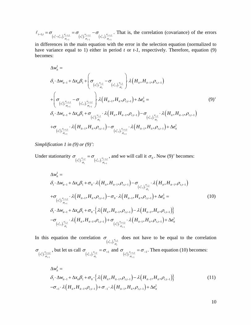
is the standard normal density function, and ( )Φ ⋅ , ( )2Φ ⋅ are the standard univariate and bivariate normal cumulative distribution functions, respectively. Equation (9) represents our more flexible correction for selectivity terms in the model in first differences and under case B. But we can present two more simplified cases for (9) if we are willing to impose some extra-assumptions. Notice that in equation (9)

( ) ( ) ( ),2 ,2 ,21 1 1 11 1

, 1, ,t t

t t t tt t

t t, t

t

ν νε ε ε ε

νσ σ σ

σ σ σ− −

−−

= = − and that

7 In fact, by assuming a linear projection of the errors in the main equation ( )ε ε −− 1

j jit it on the errors in the

selection equations in t and t-1, we do not need a trivariate normal distribution for the errors in both equations but only a bivariate normal distribution for the errors in the selection equation

.

( )ε ε ν ν−⎡ −⎣ 1 ,2 1,2, ,j j

it it it it −⎤⎦

( )ν ν,1 ,2,jit it

9

( ) ( ) ( )1,2 1,2 1,21 1 1 11 1

1 1

1,, ,t t

t t t tt t

t t ν νε ε ε ε

σ σ 1, t

t

νσ

σ σ σ− −

− −− −

−−

= = −−

−

. That is, the correlation (covariance) of the errors

in differences in the main equation with the error in the selection equation (normalized to have variance equal to 1) either in period t or t-1, respectively. Therefore, equation (9) becomes:

( ) ( )( )

( ) ( )( )

( )( )

( )

,2 ,21 11

1,2 1,21 11

1 1

,2 ,21 11

1

1 1 1 1 , 1, ,

11 , 1

, ,

1 1 1 1 , 1, ,

, ,

, ,

, ,

t tt t

t t

t tt t

t t

t tt t

t

it

it it it it t t

it it t t it

it it it it t t

w

w x H H

H H e

w x H H

ν νε ε

σ σ

ν νε ε

σ σ

ν νε ε

σ σ

δ β σ σ λ ρ

σ σ λ ρ

δ β σ λ ρ σ

−

− −−

− −

−

− −

− −

− − −

∆ =

⎛ ⎞⎜ ⎟⋅∆ + ∆ + − ⋅⎜ ⎟⎝ ⎠

⎛ ⎞⎜ ⎟+ − ⋅ + ∆ =⎜ ⎟⎝ ⎠⋅∆ + ∆ + ⋅ −

−

( )

( )( )

( )( )

1,2 1,21 11

1 1

1 , 1

11 , 1 1 , 1

, ,

, ,

, , , ,t

t tt t

t t

it it t t

it it t t it it t t it

H H

H H H H eν νε ε

σ σ

λ ρ

σ λ ρ σ λ ρ− −

−− −

− −

− − − −

⋅

+ ⋅ − ⋅ + ∆

(9)’

Simplification 1 in (9) or (9)’: Under stationarity

( ) ( ),2 1,21 11

1, ,t

t tt t

νε ε

σ σtν

σ σ−

−−

= , and we will call it 0σ . Now (9)’ becomes:

( )( )

( )

( )( ) ( )

( ) ( ){ }

( )

,211

1,21

1

11

1

1 1 1 0 1 , 1 1 ,,

11 , 1 0 1 , 1

,

1 1 1 0 1 , 1 1 , 1

,

, , , ,

, , , ,

, , , ,

tt

t

tt

t

t

it

it it it it t t it it t t

it it t t it it t t it

it it it it t t it it t t

w

w x H H H H

H H H H e

w x H H H H

νε

σ

νε

σ

ε

δ β σ λ ρ σ λ

σ λ ρ σ λ ρ

δ β σ λ ρ λ ρ

σ

−

−

−

−

− − −

− − − −

− − − −

∆ =

⋅∆ + ∆ + ⋅ − ⋅

+ ⋅ − ⋅ + ∆ =

⋅∆ + ∆ + ⋅ −

−

1ρ− −

−

( )( )

( ),2 1,21

1

11 , 1 1 , 1

,, , , ,

t tt

t t

it it t t it it t t itH H H H eν νε

σ σ

λ ρ σ λ ρ−

−

− − − −⋅ + ⋅ + ∆

(10)

In this equation the correlation

( ) ,211 , t

tt

νε

σ

σ−

does not have to be equal to the correlation

( ) 1,21

1, t

tt

νε

σ

σ−

−

, but let us call ( ) ,21

11

, tt

t

νε

σ

σ σ−

+= and ( ) 1,21

1

1, t

tt

νε

σ

σ σ−

−

−= . Then equation (10) becomes:

( ) ({ }( ) ( )

1

1 1 1 0 1 , 1 1 , 1

11 1 , 1 1 1 , 1

, , , ,

, , , ,

it

it it it it t t it it t t

it it t t it it t t it

w

w x H H H H

H H H H e

δ β σ λ ρ λ

σ λ ρ σ λ ρ

− − − −

+ − − − − −

∆ =

⋅∆ + ∆ + ⋅ −

− ⋅ + ⋅ + ∆

)ρ − (11)

10

And, therefore, independently of the temporal pair in the panel (t, t-1), the coefficients 0σ ,

1σ+ and 1σ− , are not with a time subscript, what is important for estimation because it means that with the length of the panel we do not increase the number of parameters associated to the selection correction terms to be estimated. In this case we will plug the estimated lambdas coming from the bivariate probit (biprobit in STATA) and only 3 parameters should be estimated associated to the selection correction terms. To correct for sample selection will require to increase the number of regressors in a dimension of 3. Further, if we assume an exchangeability condition like the one in Kyriazidou (1997), that is, the joint distribution functions that follow are identical

1 1 1 11 ,2 1,2 1 1,2 ,2( , , , ) ( , , , )t t t t t t t tF Fε ε ν ν ε ε ν ν− − − −= , this implies 1 1σ σ+ −= (let us call them simply

σ ) and in this case equation (11) becomes:

( ) ( ){ }( ) ( )

( ) ( ){ }( )

1

1 1 1 0 1 , 1 1 , 1

11 , 1 1 , 1

1 1 1 0 1 , 1 1 , 1

1 , 1 1 ,

, , , ,

, , , ,

, , , ,

, , , ,

it

it it it it t t it it t t

it it t t it it t t it

it it it it t t it it t t

it it t t it it t t

w

w x H H H H

H H H H e

w x H H H H

H H H H

δ β σ λ ρ λ ρ

σ λ ρ σ λ ρ

δ β σ λ ρ λ ρ

σ λ ρ λ ρ

− − − − −

− − − −

− − − − −

− − − −

∆ =

⋅∆ + ∆ + ⋅ −

− ⋅ + ⋅ + ∆ =

⋅∆ + ∆ + ⋅ −

− ⋅ − ( ){ }( ) ( ) ( ){ }

( ) ( ){ }

11

11 1 1 0 1 , 1 1 , 1

11 1 1 1 , 1 1 , 1

, , , ,

, , , , ,

it

it it it it t t it it t t it

it it it it t t it it t t it

e

w x H H H H e

w x H H H H e

δ β σ σ λ ρ λ ρ

δ β σ λ ρ λ ρ

− − − −

− − − − −

+ ∆ =

⋅∆ + ∆ + − ⋅ − + ∆ =

⋅∆ + ∆ + ⋅ − + ∆

−

(12)

where ( )0σ σ σ= − . In this case we estimate the biprobit with STATA, we estimate the corresponding lambda terms coming from the biprobit as explained before, we construct the estimated new regressor ( ) ( ){ }1 , 1 1 , 1, , , ,it it t t it it t tH H H Hλ ρ λ ρ− − − −− , and we estimate the

parameter σ that under stationarity and the joint conditional exchangeability assumption in Kyriazidou is time invariant. That means that in this case correcting for sample selection increases the dimension of regressors in only one dimension and that by increasing the length of the panel we do not increase the number of parameters to be estimated for the sample selection correction, the dimension of this parameter is one independently of the dimension of the panel length. With this we solve a sample selection correction terms parameters dimensionality problem when the T dimension in the panel was growing in the estimators in Rochina-Barrachina (1999) and Dustmann and Rochina-Barrachina (2007). Simplification 2 in (9) or (9)’: When ρ − =, 1 0t t , we have that *

, 1 1it t itM H− −= , *1,it t itM H− = ,

( ) ( ) ( ) ( ) ( ) ( ) ( ) ( )1 , 1 1 1, ,it it t t it it it it it it itH H H H H H H Hλ ρ φ φ λ− − − −= Φ Φ ⋅Φ = Φ = H and

( ) ( ) ( ) ( ) ( ) ( ) ( ) ( )1 , 1 1 1 1 1, ,it it t t it it it it it it itH H H H H H H H Hλ ρ φ φ λ− − − − − −= Φ Φ ⋅Φ = Φ = 1− .

11

Therefore, (9)’ becomes:

( )( )

( )( )

,2 1,21 11

1

1

11 1 1 1

, ,t tt t

t t

it

it it it it it

w

w x H Hν νε ε

σ σ

δ β σ λ σ λ−

−−

− −

∆ =

⋅∆ + ∆ + ⋅ − ⋅ + ∆e (13)

and the model simply has to include as new regressors correcting for sample selection the standard Heckman lambda terms coming from univariate probits in t and t-1. This is like this because when ρ − =, 1 0t t ,

1, 1 , 1 ,j j jit i it it it i it it i itE z d d E z d E z dε ε ε−⎡ ⎤ ⎡ ⎤ ⎡∆ = = = = −⎣ ⎦ ⎣ ⎦ ⎣ 1 1 1− − ⎤= ⎦ . But, which is the

restriction that (13) imposes? For ρ − =, 1 0t t it is required that the errors in the selection equation in periods t and t-1, that is ν = +,2 ,2it it iu c and ν − −= +1,2 1 ,2it it iu c , are not

correlated. The problem with panel data is that even if the ( )−1,it itu u are not correlated, the (ν ,2it ,ν −1,2it ) will be naturally correlated because of the component coming from the individual effect in the selection equation. Therefore, for simplification 2 to work, we will need also to assume that either the selection equation has not individual effects or that even if they exist in that equation the ratio of the variance from them over the global variance of the global error in that equation (

,2ic

ν = +,2 ,2it it iu c ) is small enough. Both under the more general case in (9) or the simplified cases in (12) or in (13), there will be the following need of instruments in relation to the variables itx∆ and in the model in time differences:

1itw −∆

Need of IVs for itx∆ : If we want to allow for the variables itx to be correlated with the idyosincratic error ε1it even after controlling for individual effects and sample selection in the model in time differences, we can instrument itx∆ with 2 3, ,...,it it i1x x x− − . Need of IVs for : is correlated with 1itw −∆ 1itw −

11itε − . We need something correlated with

but not with 1itw −1

1itε − .Given that we require for estimation in increments that (because we condition to a sample with

11 1it itw w− −=

1 1it itd d −= = ), if 12 2it itw w− −= , is a good

instrument for . However, if

12itw −

1itw −∆ 02it itw w 2− −= , then a good instrument for

will we the closets in time 1 01 1it it itw w w− −∆ = − 2−

1it s it sw w− −= . It could also be probably

possible to use as instrument (if it has a good correlation with 02itw −

11itw − ), but we think that

it will be probably better to choose the closets in time 1it s it sw w− −= .

Recapitulating: Under Case B, and working with time differences, we generally require bivariate sample selection correction terms (univariate Heckman’s lambda terms for our simplification 2) and we need at least 3 periods per individual.

12

2.2.2 The switching model under case A (latent dynamics switching) Under the assumption that the switching model is of the latent dynamics switching type (case A) we have:8

0 0 0

0 1 0

1 1 11 1 1

it it it i it

it it it i it

w w x

w w x

0

1

δ β α ε

δ β α ε−

−

= ⋅ + + +

= ⋅ + + + 0,1j = (14a, 14b)

* *; 1it it i it it itd z u d dγ η 0⎡ ⎤= + + = >⎣ ⎦ , (15) Because under case A dynamics come only through the same regime, even in the estimation in levels of (14a, 14b) we have to condition to 1it itd d − j= = . To illustrate our estimation procedure, which is going to combine for estimation both the model in levels and in first time differences in a type of System-GMM estimator, let us first take as example estimation in levels of (14b):

( )( )

( )( )

,2 1,21 1

1

1 1 1 11 1 1 1 ,1 1

1 11 1 1 1 1 , 1 1 , 1

, ,

, 1

, , , ,t t

t tt t

it it it i it i it it it

it it i it it t t it it t t it

w w x z E z d d e

w x z H H H H eν νε ε

σ σ

δ β ψ ν

δ β ψ σ λ ρ σ λ ρ−

−

− −

− − −

⎡ ⎤= ⋅ + + + = = + =⎣ ⎦⋅ + + + ⋅ + ⋅ +− −

, (16)

where 1

,1 1,it i it itE z d dν −⎡ = =⎣ 1⎤⎦

⎤⎦

has been derived from the three-dimensional normal distribution assumption that substitutes assumption A4 for the model in levels in case B and A4’ for the model in time differences in case B: •A4’’: The errors are trivariate normally distributed and independent of

.

1,1 ,2 1,2, ,it it itν ν ν −⎡⎣

iz Under stationarity

( ) ,21 0, t

tt

νε

σ

σ σ= and ( ) 1,21

1

1, t

tt

νε

σ

σ σ−

−

−= , and (16) becomes:

( ) ( )1 1 1

1 1 1 1 0 1 , 1 1 1 , 1, , , ,it it it i it it t t it it t t itw w x z H H H Hδ β ψ σ λ ρ σ λ ρ− − − − −= ⋅ + + + ⋅ + ⋅ + e− (17) To construct estimates of the ( )λ ⋅ terms the coefficients in the Hs will be jointly determined with ρ −, 1t t , using a bivariate probit for each pair of time periods. When ρ − =, 1 0t t , (16) becomes:

8 The estimation method we are going to develop for the latent class switching is also valid for the typical sample selection model, where either we observe or we do not observe the outcome variable, that is, we only observe the outcome variable under one regime.

13

( )( )

,21

1 1 11 1 1 1 ,1

1 11 1 1 1

,

, 1

tt

t

it it it i it i it it

it it i it it

w w x z E z d e

w x z H eνε

σ

δ β ψ ν

δ β ψ σ λ−

−

⎡ ⎤= ⋅ + + + = + =⎣ ⎦⋅ + + + ⋅ +

1

(18)

and we come back again to univariate probits per each t. We revise next the possibilities of IVs for the itx regressors, which may be endogenous, and also for the lagged variable 1itw − : Need of IVs for itx : any potential correlation of itx with α1

i coming from the correlation of

itx with is controlled for by parameterizing iz α1i as α ψ= +1

1i iz c1,1i . However, there

remain two sources of potential endogeneity for itx . First, the correlation of itx with α1i

coming from the correlation of itx with . Second, the correlation of 1,1ic itx with the

idyosincratic error ε1it even after controlling for individual effects and sample selection. Both to correct for the first and the second, the possible IVs for itx are and itz −∆ 1itx and further increments of lags (the increments are valid instruments by assuming the extra assumption coming from system-GMM, ( )∆ =1

,1 0it iE x c , (see page 136 of Blundell and Bond, 1998). Need of IVs for : is correlated with . We need something correlated with 1

1itw −1

1itw −1,1ic

11itw −

but not with . If then 1,1ic

12it itw w− = 2− −∆ 1

1itw is a valid instrument. Otherwise we can use the closest past increment in time of the type − − −∆ = −1 1 1

( 1)it s it s it sw w w +

1

. Recapitulating: Under Case A, and working with levels, we require in general bivariate probits and we need at least 3 periods per individual. Second, let us take as example estimation of (14b) in first time differences:

1 11 1 1it it it itw w xδ β ε−∆ = ⋅∆ + ∆ + ∆ (19)

We will need a sample of individuals with 1 2 1it it itd d d− −= = = , and, therefore, the sample selection correction term will come from a trivariate probit:

1 1 11 1 1 1 2,it it it it i it it it itw w x E z d d dδ β ε− −⎡ ⎤∆ = ⋅∆ + ∆ + ∆ = = = + ∆⎣ ⎦

11 e− (20) See Tallis (1961) to work it out 1

1 2,it i it it itE z d d dε − − 1⎡ ⎤∆ = = =⎣ ⎦ under a 4-variant normal distribution assumption:9

9 Which could also allow for some simplifications of the sample selection correction terms under the

14

•A4’’’: The errors are 4-variate normally distributed and

independent of . ( )1 ,2 1,2 2,2, , ,j j

it it it it itε ε ν ν ν− − −⎡ −⎣

⎤⎦

iz There will be the following need of instruments in relation to the variables itx∆ and 1

1itw −∆ in the model in time differences: Need of IVs for itx∆ : If we want to allow for the variables itx to be correlated with the idyosincratic error ε1it even after controlling for individual effects and sample selection in the model in time differences, we can instrument itx∆ with 2 3, ,...,it it i1x x x− − . Need of IVs for : is correlated with 1

1itw −∆ 11itw −

11itε − . We need something correlated with

but not with 11itw −

11itε − . Given that under case A in increments we require

, is a good instrument for 1 2 1it it itd d d− −= = = 12itw −

11itw −∆ .

Recapitulating: Under Case A, and working with time differences, we generally require sample selection correction terms that require estimation of a trivariate probit and we need at least 3 periods per individual. 2.3 Which type of switching: latent (case A) or observed (case B) dynamics?

In many cases the economic theory provides a response to this question. However, in some cases is useful to know which type of switching model the data supports. In this section we propose a very simple procedure to test between these two competing switching models. The procedure can be stated as follows: Select the sample of tree consecutive observations for each unit, and then form two samples: the sample (A) in which the sequence of the selector from the first period to the last of the three periods is [0,0,0] (or [1,1,1] ); and the sample (B) in which the sequence of the selector is (or [0 ). Sample A allows us two obtain the estimates corresponding to the latent dynamics switching model

0,0,0][1or 1,1,1]or

Aδ ; and sample B allows us to obtain the observed dynamics one Bδ . Under the null that the true switching model is of the observed dynamics switching type both are consistent but the estimator obtained using sample B is relatively efficient, since uses more information (it is less restrictive in the selection of the sample). Alternatively, under the alternative (that the true model is of the latent dynamics type), only the estimates obtained using sample A are consistent. Thus, we

assumptions of stationarity and joint conditional exchangeability, and/or under . ρ =, 0t s

15

evaluate the difference between the two sets of estimates by means of a Hausman test:10

1

1= [ ] [ ( ) ( )] [ ]A B A B A Bh avar avar 2δ δ δ δ δ δ−′− − − ∼ χ

utt

0 & > 1t1 & > 1t

)

1

(21)

3 Montecarlo experiment

In accordance with the previous section we consider the following data generating process:

= 2.75it it it i itd x z η∗ − − + + +

0 0 0 0constant 0= ( ) / (1 ) = 1it it i itw x ifβ α ε δ+ + + −

1 1 1 1constant 1= ( ) / (1 ) = 1it it i itw x ifβ α ε δ− + + −

0 0 0 0 0constant 0 1= =it it it i it itw w x if dβ δ α ε−+ + + +

1 1 1 1 1constant 1 1= =it it it i it itw w x if dβ δ α ε−+ − + +

0 1= (1it it itw w d w d+ −

0,1=;)(1= jwkwkw jitit

jit −+

where denotes the observed outcome, is a dummy which determines the precise switching model we are considering (either model 1 if or model 2 if ), and all the parameters that do not vary across the experiments are set to fixed values. Apart from this we set and , and parameterize the autoregressive coefficient as

w k1=k 0=k

0constant = 2β 1

constant = 1β

0= = 1δ δ −δ . An interesting subcase of the analysis is the static switching regression model which can be obtained by imposing the restrictions: = 0, = 0,1j jδ . In addition to two versions of the switching model we also consider the possibility of a single equation model or model 3.

(22) constant

constant 1

= ( ) / (1 ) = 1= >

it it i it

it it it i it

w x iw w x i

β α ε δβ δ α ε−

− + + −+ − + + 1

f tf t

Regarding the errors, we consider the following structure for them:

: (0, ), = 2i N η ηη σ σ : (0, )it uu N σ : (0, ), = 2i N α αα σ σ : (0, ); = 2it N ε εε σ σ : (0, ); = 2 = 0,1j

i j jN jα αα σ σ

0 0 00 0= ; : (0, );it it it itv u v Nε ρ σ σ− = 2

10 Alternatively, a Sargan-difference test of overidentifying restrictions can be also constructed.

16

1 1 11 1= ; : (0, );it it it itv u v Nε ρ σ σ+ = 2

Note that and thus ( , ) = ( )jit it itcov u var uε ρ

2( , ) =

1j

it itcorr u ρερ+

, . We initially set = 0,1j

0.5=ρ . And, finally, we consider the following processes for the regressors: : (0, ); = 2it z zz N σ σ 0 0 1 1= (0.5 [ 2 ] ) / (1 ) = 1it it i it i it itx v v s u if tκ α α ρ ϖ γ+ + − − + + − 0 0 1 1

1= .5 [ 2 ] > 1it it it i it i it itx x v v s u if tγ κ α α ρ ϖ−+ + + − − + + : (0, ); = 2it x xNϖ σ σ

where κ is a parameter that controls whether or not x is exogenous in the model and is a dummy that determines whether or not x is correlated with the error in the selection equation. In addition, we initially set

s

0.5=γ . In summary we consider a three equations model in which we allow for variation in the dynamics of the outcome variable and the various correlation parameters of the model. As a distinct feature of our simulations we explicitly consider the case in which one of the regimes ( ) is a low probability event. In particular, given the parameters of the selection equation, the probability that is set around 0.15.

=1d=1d

3.1 Description of the experiments

For each experiment 1000 (or, alternatively 500) units are considered. For each unit, 20 times series observations are drawn. However, the initial 13 observation are discarded to diminish the influence of the initial conditions. Thus, we end up having a small T panel data sample as it is usual in the empirical literature. After the realization of the selector, the regime panels are formed. At least three consecutive observations of the same regime are needed in order to form an observation of the selected panel (of either regime) in the case of model 1 (A). Alternatively in the case of model 2 (B), provided that , only two consecutive observations of the same regime are needed. Due to the fact that the probability of being equal one is small, the regime 1 panel is discarded for the estimation stage. However, this does not have severe consequences for the testing procedures since the testing of the switching against the single model can be performed using the estimates of the pooled and the high probability regime sample. For each combination of the parameters we made 100 replications.

1>t

d

In cases where is not exogenous, we select the instruments as follows. For the case of the Arellano-Bond (AB-est) estimator we first use lags from

x2−t to 4−t , although we also

compare the performance of the estimates when extending the instrument set with further lags.11 In the System-GMM (SYS-est) estimator we additionally use first differences of the 11In fact, GMM could theoretically imply that we should use as many instruments as possible, although it could affect to the performance of the estimation method, power of the tests and degrees of freedom

17

regressors. Should be decided about the exogeneity of we carry out, in a previous step, a Hausman and Griliches's (1986) type of test (see the empirical illustration of the paper for an example).

x

4 Preliminary Monte Carlo results

For each experiment, we present the mean bias and the standard deviation of the estimates of two parameters δ and β in the pooled sample (single equation estimates) and in the regime 0 or high probability sample. We also present results for two tests: the test of selection and the test of equality of coeficients, for the two GMM estimators considered (AB-est and SYS-est). We estimate the selection equation under four hypothesis for the case in which we impose no correlation between the regressor and the error term and we only present two for the case where correlation is allowed for.12 We consider four cases for the generation of the additional regressor X : (0) , (1) , (2)

, and (3) . However, note that when 0 1 2= = = 0s s s 1 2= =s s 0

2 = 0s 1 = 0s 0=κ , cases (iii) and (iv) are redundant, since they are identical to case (ii). We first consider the case of a pure autoregressive model for three different values of the autorregresive parameter 0( = 0.1,0.25,0.50)δ . We consider up to three specifications for the single equation model (basic specification as in (22), basic specification + a control for

, basic specification + a control for d instrumented with lags). Note that when d 0 = 0.5δ the single and the regime equations are identical except for the constant. 0 The results are, as a rule, satisfactory. However, we want to highlight the following, sometimes surprising, findings.

• When the null of a single equation model (model 3) is true, all the estimators and models show little or no bias at all.

• The bias of the single equation estimate depends on the choice of the DGP for the switching model (either model 2 of 3). For example when 0 = 0.10δ the bias is more important for model 2 than for model 1 (the pure autoregressive switching model or latent switching). Alternatively, when 0 = 25δ , the bias for model 1 is more important than it is for model 2.

= 0.5δ • When we find the most striking results. While the mean bias (with respect to

remaining. 12 In our practical application of the methods proposed in section 2 we experiment a little with the estimation of the selection equation. Therefore, we estimate the selection equation by four different parametric ways, although we always assume normality of the errors of this equation. The four procedures are: i) a probit model for each time period without accounting for correlated heterogeneity; ii) a random effects probit model; iii) a year by year probit in a reduced form allowing correlation between regressors and unobserved effects; iv) a year by year probit with the correction suggested by Wooldridge (2004).

18

0δ of the e of stimate δ ) is very small for the case of model 2 (the observed switching del) it is very import t for the case of model 1 (the latent switching model). This is true

even when we control for the variation in the constant (by adding d ) and instrumenting it.

mo an

The results also are, as a rule, very satisfactory when an addition l exogenous regressor is aincluded in both the outcome and selection equations. That is the case when 0=κ and

0 = 0.25δ (see Table 2). The estimates of δ and β show small or negligible bia r the el and significant biases for th altern ive model (outcome models 1 or 2).

Likewise, Table 3 shows that both the variable addition and the equality of coefficients tests go in the correct direction with some exceptions (specially when x follows a white noise process).

ses fotrue mod e at

The results are also satisfactory, specially regarding the bias of β , when is endogenous e n

xto the wage equations (cases 0 and 1 for the DGP of x ) or th wage a d the selection equation (case 2). However, they are still satisfactory when x is only correlated with the time invariant error component (case 3), specially in the case of the AB estimator. This is clearly due to a problem of poor instruments. For example when we extend the specification of x with additional exogenous regressors and use it as instrument in the outcome equations the bias decreases notoriously in all cases. As a matter of example we present in Table 4 and 5 the bias and testing results respectively, for the case of 0.25=κ and = 0.25δ and the reduced form year-by-year probit and Wooldridge's proposal. Note, firstl gardless of the bias in the estimate of y, that re β the equality of test is still able to provide a correct response; and, secondly, in a non-negligible number of cases the AB-est method performs better that the, in principle, more efficient system estimator. It seems that extending the model with equation in levels helps in improving the efficiency of the estimates, although it is not so clear what the result is with respect to consistency.

19

Table 1: Bias results with respect to 0δ for the pure autoregressive model: model

(1) for with x 0=κ , Correction method: year-by-year Probit.

Model Single equation estimates Regime 0 estimates eq (22) (22) +

dummy for d(22) +

inst.

d

ffor w

SYS-

est AB-est

SYS-est

AB-est

SYS-est

AB-est

SYS-est

AB-est

= 0.1δ (1) bias

.029536

.042682

.036339

.049291

.037144 .054574 .000868 .005811

s.e. .032167

.035332

.025250

.028173

.029449

.032939 .023752 .032448

(2) bias -.134225

-.130011

-.137760

-.131378

-.134703

-.124958

-.003749

.004788

s.e. .020852

.028106

.022151

.028734

.022094

..029385

.025981 .027442

(3) bias -.000094

.000322

-.002781

-.000620

-.00440

.001107 -.002490

.002898

s.e. .018784

.027438

.017957

.022267

.017839

.022500 .022639 .035809

= 0.25δ (1) bias

.140778

.149689

.133406

.140660

.134343 .145466 .000791 .008775

s.e. .027534

.031084

.026357

.032256

.025387

..032511

.026012 .037962

(2) bias -.089381

-.085653

-.094162

-.08738

-.093084

-.083003

-.022573

.007424

s.e. .020583

.029324

.020517

.026947

.020749

..027339

.031352 .033955

(3) bias .000164

.001181

.000450

.002191

-.000577

.004533 -.002960

.004858

s.e. .019993

.031933

.016842

.023984

.017042

..024552

.024747 .044271

= 0.5δ (1) bias .30294

.330340

.312666

.337514

.304715 .355254 .000634 .022282

s.e. .023295 .031967

.023295

.031967

.027437

..035036

.030695 .052295

(2) bias -.02528 -.020344

-.018041

-.012973

-.017727

-.007549

-.130647

.010503

s.e. .02128 .039445

.020440

.036464

.020817

..037052

.036735 .066057

(3) bias -.00411 -.000763

-.004186

-.000902

-.006524

.006297 -.005637

.018570

s.e. .02191 .037606 .021938 .037584 .022880 ..038801 .035546 .062272

20

Table 2: Bias Results for the model with exogeneous regressors: = 0.25δ , 0=κ

True model Single equation estimates Regime 0 estimates

for SYS-est

AB-est SYS-est

AB-est

w X stat δ β δ β 0δ 0β 0δ 0β correction method: Y-b-Y probit

(1) 0 bias .1759 .1234 .1823 .1309 -.0011

-.0014

.0010 -.0020

s.e. .0193 .0405 .0236 .0431 .0224 .0281 .0313 .0318 1 bias .1338 .2222 .1423 .2182 .0006 .0011 .0068 .0015 s.e. .0256 .0447 .0313 .0526 .0233 .0235 .0332 .0283

(2) 0 bias -.065 .2990 -.063 .3001 -.013 -.005 .0029 -.000 s.e. .0170 .0263 .0221 .0276 .0198 .0224 .0242 .0255 1 bias -.107 .3521 -.104 .3398 -.015 .0031 .0046 .0034 s.e. .0227 .0290 .0316 .0360 .0233 .0251 .0268 .0309

(3) 0 bias .0005 .0013 .0026 .0020 .0012 .0035 .0061 .0049 s.e. .0143 .0167 .0192 .0192 .0263 .0225 .0341 .0280 1 bias -.002 .0041 .0001 .0050 -.003 .0057 .0028 .0089 s.e. .0159 .0180 .0240 .0198 .0230 .0263 .0409 .0288

correction method: Reduced Form Random effect probit (1) 0 bias .1831 .1330 .1863 .1409 .0015 -.002 .0047 -.000

s.e. .0200 .0386 .0242 .0424 .0210 .0231 .0298 .0277 1 bias .1261 .2398 .1330 .2369 .0009 -.000 .0012 -.000 s.e. .0311 .0486 .0351 .0582 .0271 .0271 .0348 .0323

(2) 0 bias -.071 .3115 -.070 .3128 -.012 -.004 .0051 .0007 s.e. .0205 .0252 .0274 .0287 .0216 .0258 .0266 .0301 1 bias -.118 .3652 -.112 .3479 -.018 .0027 .0053 .0019 s.e. .0223 .0323 .0341 .0341 .0226 .0291 .0302 .0329

(3) 0 bias -.000 .0042 .0019 .0050 -.001 .0059 .0056 .0100 s.e. .0144 .0180 .0217 .0200 .0218 .0263 .0349 .0313 1 bias .0002 .0032 .0023 .0038 -.001 .0086 .0072 .0105 s.e. .0176 .0186 .0195 .0205 .0225 .0265 .0341 .0292

correction method: Reduced Form Y-b-Y probit (1) 0 bias .1787 .1354 .1807 .1440 .0019 -.065 .0050 -.065

s.e. .0241 .0371 .0283 .0407 .0241 .0237 .0301 .0290 1 bias .1279 .2344 .1365 .2269 .0125 -.059 .0190 -.062 s.e. .0237 .0468 .0314 .0486 .0245 .0274 .0399 .0302

(2) 0 bias -.075 .3098 -.071 .3101 -.016 -.073 .0028 -.066 s.e. .0191 .0285 .0286 .0287 .0229 .0257 .0265 .0288 1 bias -.117 .3686 -.116 .3508 -.007 -.053 .0140 -.060 s.e. .0202 .0326 .0304 .0362 .0229 .0253 .0284 .0299

(3) 0 bias .0005 .0043 .0023 .0046 -.001 .0054 .0033 .0061 s.e. .0154 .0168 .0186 .0194 .0209 .0226 .0311 .0255

21

1 bias .0003 .0029 .0043 .0041 -.003 .0053 .0056 .0046 s.e. .0154 .0173 .0191 .0191 .0266 .0232 .0371 .0290

correction method: Wooldrigde's correction (1) 0 bias .1778 .1317 .1819 .1404 -.002 -.052 .0040 -.050

s.e. .0237 .0386 .0287 .0426 .0230 .0296 .0345 .0345 1 bias .1266 .2387 .1344 .2313 -.000 .0094 .0066 .0108 s.e. .0225 .0455 .0290 .0519 .0229 .0285 .0337 .0321

(2) 0 bias -.075 .3142 -.070 .3140 -.016 -.057 .0039 -.051 s.e. .0195 .0307 .0282 .0341 .0203 .0253 .0263 .0273 1 bias -.117 .3645 -.112 .3472 -.017 .0041 .0074 .0020 s.e. .0199 .0294 .0327 .0326 .0243 .0272 .0266 .0316

(3) 0 bias .0011 .0025 .0047 .0038 -.002 .0048 .0064 .0072 s.e. .0135 .0158 .0199 .0188 .0221 .0233 .0320 .0298 1 bias -.000 -.000 .0015 -.000 -.002 -.000 .0058 .0013 s.e. .0150 .0161 .0204 .0177 .0244 .0242 .0363 .0283

Table 3: Mean significance of the variable addition and equality of coefficients test, = 0.25δ , 0=κ

True model Correction method year-by-year-

Probit Correction method RE Probit

for

Var. addition test

Eq. of coeff. test

Var. addition test

Eq. of coeff. test

w X SYS-est AB-est

SYS-est AB-est

SYS-est AB-est

SYS-est AB-est

(1) 0 0.0002 0.0005 0.0000 0.0006 0.0014 0.0022 0.0000 0.0006 1 0.0004 0.0020 0.0000 0.0025 0.0004 0.0008 0.0000 0.0014

(2) 0 0.0001 0.0005 0.0000 0.0000 0.0002 0.0004 0.0000 0.0000 1 0.0000 0.0001 0.0000 0.0000 0.0003 0.0011 0.0000 0.0000

(3) 0 0.2711 0.2786 0.7992 0.7082 0.2601 0.2609 0.8065 0.7301 1 0.2481 0.2502 0.8080 0.7077 0.2517 0.2488 0.8179 0.7122 Model Correction method RF y-b-y

Probit Correction method:

Wooldrigde's corr. for Var.

addition test Eq. of

coeff. test Var.

addition test Eq. of

coeff. test w X SYS-est AB-

est SYS-est AB-

est SYS-est AB-

est SYS-est AB-

est (1) 0 0.0135 0.0213 0.0000 0.0001 0.1854 0.1804 0.0000 0.0040

1 0.0178 0.0235 0.0000 0.0001 0.0031 0.0025 0.0000 0.0014 (2) 0 0.0036 0.0064 0.0000 0.0000 0.2047 0.2130 0.0000 0.0000

1 0.0222 0.0146 0.0000 0.0000 0.0017 0.0029 0.0000 0.0000 (3) 0 0.2223 0.2358 0.8103 0.7651 0.2712 0.2631 0.8395 0.7127

1 0.2566 0.2522 0.8092 0.7324 0.2395 0.2368 0.8220 0.7067

22

Table 4: Bias Results: = 0.25δ , 0.25=κ

True model Single equation estimates Regime 0 estimates for SYS-est AB-est SYS-est AB-est

w X stat δ β δ β 0δ 0β 0δ 0β correction method: Reduced form Y-b-Y probit

(1) 0 bias .1670 .0214 .1707 -.005 -.001 -.283 .0068 -.284 s.e. .0223 .6352 .0263 .7851 .0203 .1588 .0233 .1658 1 bias .1380 .0851 .1542 .0468 .0121 -.068 .0380 -.126 s.e. .0264 .1081 .0324 .1342 .0237 .0744 .0302 .0784 2 bias .1305 .0732 .1440 .0422 .0206 -.092 .0502 -.166 s.e. .0278 .1117 .0364 .1384 .0250 .0699 .0331 .0812 3 bias .1117 .2584 .1327 .2067 -.005 -.060 .0195 -.038 s.e. .0307 .1254 .0392 .1873 .0270 .0789 .0324 .0836

(2) 0 bias -.071 .2599 -.063 .2484 .0257 -.276 .0036 -.269 s.e. .0200 .3057 .0284 .3449 .0179 .1995 .0179 .1730 1 bias -.136 .5346 -.123 .5178 .0092 .0366 .0078 -.041 s.e. .0253 .0815 .0364 .0945 .0238 .0700 .0209 .0612 2 bias -.132 .5087 -.117 .4903 .0158 -.009 .0135 -.072 s.e. .0246 .0867 .0342 .1128 .0297 .0900 .0232 .0729 3 bias -.193 .6262 -.152 .5494 -.013 .0462 .0080 -.002 s.e. .0330 .0896 .0457 .1231 .0290 .0909 .0214 .0719

(3) 0 bias -.001 -.217 -.000 -.215 -.002 -.196 .0030 -.221 s.e. .0129 .2061 .0164 .2044 .0178 .1743 .0212 .1580 1 bias .0050 -.026 .0159 -.046 .0103 -.067 .0377 -.119 s.e. .0192 .0665 .0246 .0733 .0290 .0868 .0358 .0895 2 bias .0042 -.015 .0137 -.033 .0114 -.048 .0411 -.105 s.e. .0240 .0646 .0299 .0753 .0302 .0784 .0363 .0875 3 bias -.002 -.004 .0026 -

.0050 -.007 -.031 .0142 -.010

s.e. .0184 .0486 .0271 .0513 .0277 .0646 .0358 .0749 correction method: Wooldridge's proposal

w X stat δ β δ β 0δ 0β 0δ 0β (1) 0 bias .1679 .1272 .1709 .0822 .00141 -.035 .0034 -.061

s.e. .0229 .5844 .0275 .6709 .0179 .1208 .0232 .1174 1 bias .1310 .1113 .1448 .0807 .0077 -.045 .0329 -.103 s.e. .0287 .1133 .0386 .1392 .0269 .0736 .0325 .0795 2 bias .1270 .0622 .1394 .0376 .0184 -.092 .0430 -.146 s.e. .0247 .1063 .0322 .1368 .0272 .0814 .0359 .0919 3 bias .1238 .2700 .1510 .2003 -.008 -.071 .0167 -.017 s.e. .0325 .1498 .0395 .2162 .0316 .0847 .0368 .0892

(2) 0 bias -.071 .2768 -.063 .2556 .0205 -.020 .0025 -.043 s.e. .0185 .3744 .0255 .3738 .0172 .1596 .0188 .1537 1 bias -.137 .5184 -.120 .5012 .0109 .0229 .0073 -.047

23

s.e. .0250 .0793 .0318 .1003 .0283 .0890 .0241 .0749 2 bias -.130 .5167 -.114 .4931 .0221 -.015 .0110 -.056 s.e. .0270 .0803 .0378 .0976 .0288 .0893 .0252 .0703 3 bias -.197 .6199 -.165 .5565 -.024 .0085 .0049 .0023 s.e. .0280 .0846 .0427 .1143 .0272 .0741 .0254 .0615

(3) 0 bias -.001 -.244 .0001 -.243 -.003 -.220 .0027 -.214 s.e. .0132 .2113 .0171 .2304 .0186 .1116 .0249 .1138 1 bias .0050 -.026 .0159 -.046 .0103 -.067 .0377 -.119 s.e. .0192 .0665 .0246 .0733 .0290 .0868 .0358 .0895 2 bias .0023 -.014 .0108 -.030 .0110 -.055 .0389 -.106 s.e. .0184 .0521 .0256 .0596 .0266 .0663 .0396 .0835 3 bias -.000 -.011 .0064 -.015 -.005 -.076 .0192 -.026 s.e. .0200 .0505 .0298 .0557 .0321 .0704 .0431 .0771

Table 5: Mean significance of the variable addition and equality of coefficients test,

= 0.25δ , 0.25=κ

Model Correction method RF YBYP Correction method RF YBYP+WC for var ad.

test Eq of

coef. var ad.

test Eq of

coef. w X SYS-est AB-est SYS-est AB-est SYS-est AB-est SYS-est AB-est

(1) 0 .06974 .0679 .0002 .0009 .2172 .2232 .0001 .0005 1 .13512 .0992 .0005 .0058 .1037 .0811 .0006 .0061 2 .18790 .1312 .0005 .0035 .1427 .1028 .0007 .0041 3 .06459 .0454 .0009 .0281 .0467 .0453 .0007 .0355

(2) 0 .06535 .0585 .0013 .0799 .1935 .2096 .0016 .1178 1 .21336 .1261 .0015 .0001 .1499 .0843 .0022 .0002 2 .24784 .1780 .0010 .0008 .1706 .1283 .0014 .0011 3 .15215 .0325 .0003 .0012 .0856 .0277 .0002 .0010

(3) 0 .27130 .2694 .7153 .6065 .2327 .2398 .6278 .5549 1 .16792 .2429 .7307 .5522 .1831 .2344 .7055 .5408 2 .16792 .2429 .7307 .5522 .1831 .2344 .7055 .5408 3 .26702 .2732 .0669 .6796 .2616 .2606 .0395 .6543

5 An economic example: strikes and wages

The literature on the relationship between strike and wage outcomes has two strands. The first strand argues that strikes are accidents, or mistakes, that occur during bargaining (Siebert and Addison (1981)). The second strand, inspired on the seminal work of Hicks (1932), stresses a negative relationship or concession schedule between the length of a strike and wage settlement. On very rare occasions the possibility of different wage-strike regimes has been called into

24

question, though. Among the few exceptions we can mention, from a theoretical point of view, Cramton and Tracy's (1994) wage bargaining model with time varying threats, they stress that employees could take other action besides strikes, and that these actions may lead to different wage equations; and, from the empirical point of view, Stengos and Swidinsky (1990) who find empirical evidence of small strikers' wage premium in Canada. In the empirical literature, see Cramton and Tracy (2003) for a review, there is very contradictory evidence on the slope of the wage concession curve as well as on the implicit wage premium (or cost) from a strike. Furthermore, it is still unclear the dynamic nature of the wage process, or, more importantly, whether one or two-wage equations should be specified. The aim of this paper is to seed some light on these issues. With these purposes, our work combines a careful treatment of the endogeneity of dispute variables in dynamic wage settlement equations in a panel data context with a room open to segregate wage equations for each strike regime. The estimation and subsequent test of the latter possibility becomes of crucial importance, since the rejection of a single, common equation for both strike regimes invalidates standard single-equation estimates. In a sense, this would be a very negative result and a warning for future work in estimating panel data models in presence of an endogenous treatment dummy variable and when the (endogeneously) treated sample is relatively small. Yet we are able to obtain consistent estimates of one of the regimes, the non-strike regime in our case.

5.1 Specification and variables

A vast majority of the recent models postulate that the duration of the negotiation threats (either the length of a strike, the holdout period or even a mixed threat) is determined by the time needed to credibly establish that the employer's demand price for labor is no higher than the true one. Then, the wage settlement splits the difference between the demand and supply prices. Card (1990b), Cramton and Tracy (1994) and Cramton, Gunderson and Tracy (1999) provide recent examples in a non-dynamic context.13 All of them agree on the idea that longer strikes would, in general, produce lower observed wages. In our benchmark equation (see Kennan and Wilson, 1989), the wage change settlement ( ) depends linearly on strike variables (strike indicator and duration ), observed variables ( ) and an unobserved component. The unobserved part has two components. The first component or bargaining pair heterogeneity effect (

w d durx

iα ) randomly varies across observations. The second component (ε ) shifts firm valuation. Summarizing,

= ,i d i dur i i i iw d dur xδ δ β α ε+ + + +

where d takes the value one if a strike is observed and zero otherwise, and dur is the realized length of a work stoppage, which is jointly determined with the wage settlement. Note that can be thought of as the maximum wage change available for workers, i.e., a corner solution for the strike wages. Furthermore, from standard strike

( = 0w dur )

13See Cramton and Tracy (2003) for a comprehensive overview of these models (with the addition of recent developments) and applications.

25

theory (Hicks, 1932) it is expected that < 0durδ . In a single equation context, the empirical evidence using panel data is puzzling. While Card (1990b) finds no systematic relationship between wage outcomes and strike variables, the evidence found by McConnell (1989) is just the opposite. In both cases a control for bargaining pairs heterogeneity is introduced, but the strike variables are treated as strictly exogenous. Jiménez-Martín (1999) shows that it is not only necessary to control for unobserved heterogeneity but also for endogeneity. When those problems are controlled for, a strong negative correlation between the strike duration and the wage is evidenced. Stengos and Swidinksy (1990) considered the possibility of two distinct wage regimes,14 one for each strike regime and found evidence of selection induced by the strike indicator, and behavioral differences between both strike regimes. However they neither consider (because of data limitations) the effect of the strike duration in the strike wage equation nor exploit the dynamic nature of the negotiation process. Thus, we consider both a two-equation framework and the possibility of wage dynamics:

(23) 0 0 0 0

0 1 0=it it it i it i itw w x for t s t dδ β α ε− + + + . . = 0;. = 1; (24) 1 1 1 1 1

1 1 1= .it dur i it it i it i itw dur w x for t s t dδ δ β α ε−+ + + + where the strike indicator, ( ), determines whether the strike wage ( ) or the non-strike wage ( ) is observed, and denotes all the observations for which d=j; j=0,1 and

is a function of the previous wages.

*= 1( )id d 1iw

0iw j

it0

1−itw Regime switching is driven by the strike model of d , which is given by

*

it it i itd z uγ η= + + (25) where z is a vector of strictly exogenous regressors, iη is an heterogeneity effect and is an error term.

itu

We allow for correlation between and the error term. Furthermore, and can be correlated.

x itu ; = 0,jit jε 1

Following our suggested methodology, we estimate the wage equations by using the Arellano and Bond (1981) GMM-IV estimation method and the selection equation by means of a reduced-form year-by-year probit. See the appendix for a description of the data and the variables as well as a short description of negotiation procedures in Spain.

14This possibility has been recently considered by Cramton and Tracy (1994) who analyze a model with two threats (strike and delay), each of them leading a different wage equation.

26

5.2 Results

he test for over-identifying restrictions shows e adequacy of the set of instruments used.

mented model using the Mill's ratio rejects the null of the absence of sample selection bias.

The results of estimating the wage change equations are reported in Table 6. We have performed a formal test for the absence of heterogeneous effects, which has been rejected in columns 2 and 5. Thus, there is sound evidence against the validity of level estimates. As for the estimates obtained from the differenced equations, they completely pass the standard specification test. We find first order serial correlation as well as the absence of second order serial correlation. Jointly, they both imply that the error in levels is white noise (Arellano and Bond, 1991). Finally, tth In the rest of Table 6 we report the estimates obtained by considering the possibility of two different wage equations, one for each strike regime. Column 3 and 4 report level estimates of the strike and non-strike wage change equations, respectively. A Wald test rejects the null hypothesis of equal coefficients (excluding those of the strike variables) between these two equations. In fact, relevant differences in the key coefficients can easily be detected. However, we must be cautious because of level estimates are likely to be inconsistent. Using the non-strike sample, a formal test for the nonexistence of bargaining pair heterogeneity effects is rejected, invalidating the non-strike level estimates (that is those reported in column 4). Consequently, we obtain a very negative result since fully consistent estimates are only obtainable using the non-strike sample (see column 5). In addition, we reject the null of equal coefficients between those obtained using the pooled sample and those obtained using non-strike observations, which implies that the non-strike and the strike equations are different. Finally, the variable addition test on the aug

27

Table 6: Wage change determination and strike outcomes.

All All Strike Non-strike Non-strike levels 1st dif levels levels 1st dif Coef. t-st. coef. t-st. coef. t-st. coef. t-st. Coef. t-st. Constant -0.91 (1.53) -0.75 (5.85) -0.69 (0.55) -0.17 (0.24) -0.97 (6.08) Lagged wage change 2,* 0.36 (15.6) -0.03 (0.76) 0.36 (8.06) 0.38 (15.0) -0.24 (4.64) difference claim-offer *2,* 0.03 (5.61) 0.03 (4.25) 0.04 (3.38) 0.01 (0.66) 0.04 (4.42) strike indicator 2,* 0.23 (1.96) 0.56 (4.78) -- -- -- strike duration 2,* -.012 (5.69) -.030 (5.58) -.018 (1.96) Selection term - - -0.39 (3.66) 0.03 (1.83) 0.046(2.31) Cost of living allowance signed 3 -0.10 (1.35) -0.41 (4.73) -0.09 (0.47) -0.05(0.56) -0.28 (1.70) lagged employment *3,* -0.02 (1.01) -0.86 (1.34) -0.02 (0.47) -0.05 (1.93) -1.98 (2.65) lagged relative wage *3,* 0.10 (1.53) -0.98 (2.58) -0.12 (0.73) 0.12 (1.04) 0.39 (0.92) Change of the value added *2,* 0.05 (0.39) 0.11 (1.02) 0.32 (1.22) 0.14 (1.04) -0.45 (2.51) Real lagged profits per employee *2,* 0.08 (0.59) 1.21 (2.75) 0.75 (1.97) 0.06 (0.42) 0.94 (2.40) 1 if lagged profits 0> 0.33 (5.16) 0.43 (3.80) 0.42 (2.45) 0.27 (3.44) 0.08 (0.62) Sample/obs all/1131 all/521 strike/162 no-st./969 No-st./370 Wald (df) 4 720.6 (26) 1185.2 (26) 821.0 (26) 596.6 (26) 911.3 (25) Sargan (df) 5 115.9 (101) 79.1 (74) 38.8 (37) 84.3 (80) 68.8 (60) Fosc 6 (obs) -0.86 -4.03 -- -0.32 -2.11 Sosc 6 (obs) 1.84 0.76 -- 1.10 0.05 Exogeneity of strikes outcomes 7 -- 33.1(2) -- Effects test 8 -- 47.63(27) -- -- 22.80(12) Wald column (2) vs (5) 9 -- -- 41.11(22) id with omitted dummies 94.43(28)

others controls: works' council structure variables, industry and market controls, spillover and price controls, share of capital owned by foreigners and by the public sector, % sales in the domestic market

notes: (1) All the columns consider year, quarterly and industry dummies. (2) Lags of these variables have been used as GMM instruments (-1) (-2) and earlier lags in the level (1st diff.) models. (3) Instrumented by using their lagged value (levels) or their lagged difference (first differences). (4) Wald test of the null that the vector of coefficients (excluding time and industry dummies) is

zero. (5) Test of the validity of the set of instruments. Under the null of adequacy, the test is distributed as , where 2rχ r is the number

of overidentifying restrictions. (6) Test of the absence of first (second) order serial correlation in the error term (Arellano and Bond, 1991). (7) Hausman test (Griliches and Hausman, 1986) comparing estimates obtained under the null of exogeneity and the alternative of predeterminedness. (8) Sargan difference test (Arellano, 1993), under the null hypothesis that both the level and differenced models

provide consistent estimates it is distributed as a , where 2rχ r is the number of additional overidentifying restrictions implied by the

levels model. For the set of variables marked with * we have tested overidentifying restrictions like 1( ) =it tE x 0ε− and for those

marked with ** we have tested 1( ) =it tE x 0ε−∆ , being a levels error. (9) Wald test of the hypothesis that the coefficients,

excluding the strike variables and the selection term, of columns i and are equal. In the first row we test all the variables whose coefficients are reported in the table as well as other controls, whereas in the second row time and industry dummies are also considered.

tuj

28

6 Concluding remarks In this paper we present estimators for panel data sample selection and switching models where the regression equations are dynamic and it is allowed for the existence of endogenous regressors and correlated individual unobserved heterogeneity. We consider two types of switching models under the names of observed dynamics switching and latent dynamics switching. The dynamic sample selection model implicitly assumes an underlining latent dynamics switching regime process. The type of methods presented are different Generalized Method of Moments (GMM) estimators for dynamic panel data sample selection and switching models that may combine estimation of the models both in first time differences and in level equations (with the corresponding sample selection correction terms under one or the other case). Therefore, we consider the possibility of applying System-GMM estimators for dynamic panel data to the case of sample selection and switching models. Depending both on estimation in levels or time differences and on the types of switching models considered (observed or latent) the sample selection correction terms present different degrees of complexity. Some of this complexity can be simplified if we are willing to impose stationarity assumptions, exchangeability conditions, and/or lack of individual heterogeneity in the selection equations determining the switching regimes. In the general setting neither stationarity, exchangeability, or lack of individual heterogeneity in the selection equations are imposed. To see the performance of the proposed estimators we perform a Monte Carlo study of the finite sample properties of different Generalized Method of Moments (GMM) estimators for dynamic panel data sample selection and switching models. Finally, we present an empirical example using Spanish data on wage settlements and strike outcomes. In an economic context in which workers may strike to obtain a wage concession, the strike decision is endogenous to the wage process and the wage equation is then affected by endogenous selection. We test this as well as alternative economic hypotheses in a dynamic context. The results from our modest Monte Carlo Experiments show that the combination of a consistent estimator (or a consistent correction of the estimates) for the selection equation and a consistent estimator for the equation of interest performs reasonably well in estimating dynamic panel data sample selection models as well as in discriminating switching dynamic panel data sample selection models. However, further work is needed to extend our Monte Carlo for covering all the methods we have presented in our theoretical section in this paper.

References Arellano, M. (1993), "On the Testing of Correlated Effects with Panel Data," Journal of

Econometrics, 59, 87-97. Arellano, M. and Bond, S. (1991), "Some Tests of Specification for Panel Data: Monte Carlo

Evidence and an Application to Employment Equations," Review of Economic Studies, 58, 277-297. Arellano, M. and Bover O. (1995): "Another Look at the Instrumental-Variable Estimation of

Error-Components Models" Journal of Econometrics, 68, 29-51.

29

Baltagi, B. (2005): Econometric Analysis of Panel Data, John Wiley and Sons, Chichester Blundell, R. and Bond, S. (1998) "Initial Conditions and Moment Restrictions in Dynamic Panel

Data Models", Journal of Econometrics, 87, 115-143. Card, D. (1990), "Strikes and Wages: A Test of an Asymmetric Information Model," Quarterly

Journal of Economics, 105, 625-659. Charlier, E., Melenberg, B. and van Soest, A. (2001), "An analysis of housing expenditures using

semiparametric methods and panel data", Journal of Econometrics, 101, 71-107. Cramton, P. and Tracy, J. (1994), "Wage Bargaining with Time-varying Threats" Journal of

Labor Economics, 12, 594-617. Cramton, P., Gunderson M. and Tracy, J. (1999) "The effect of Collective Bargaining Legislation

on Strikes and Wages," Review of Economics and Statistics, 81, 475-487. Cramton, P. and Tracy, J. (2003) "Unions, Bargaining and Strikes" in J.T. Addison and C.

Schnabel (eds.) International Handbook of Trade Unions, Cheltenham, UK: Edward Elgar, Chapter 4, forthcoming.

Dustman, C. and Rochina-Barrachina, M. R. (2002) "Selection Correction in Panel Data Models:

An Application to Labour Supply and Wages" IZA WP 162. Gonzalez-Chapela, J. (2004), On the price of recreation goods as a determinant of female labor

supply, mimeo. Griliches, Z.and Hausman, J.A. (1986), "Errors in Variables in Panel Data," Journal of

Econometrics, 31, 93-118. Heckman, J.J. (1976), "The Common Structure of Statistical Models of Truncation, Sample

Selection and Limited Dependent Variables as a Simple Estimator for such Models," Annals of Economic and Social Measurement, 5, 475-92.

Hicks, J.R. The Theory of Strikes, London: MacMillan Press, 1932. Holtz-Eakin, D. (1998), "Testing for Individuals Effects in Autoregressive Models," Journal of

Econometrics, 39, 297-307. Hu, L. (2002), "Estimation of a Censored Dynamic Panel data model", Econometrica. 2499--

2517. Jensen et al. (2001) Jiménez-Martín, S. (1995), "The incidence, Duration and the Wage change Effect of a Strike:

Evidence from the Spanish NCGE survey," D.T. 113/1995, Madrid, FIES. Jiménez-Martín, S. (1998), "On the Testing of Heterogeneity Effects in Dynamic Panel Data

Models ", Economic Letters, 58, 157-163. Jiménez-Martín, S. (2006), "Strike Outcomes and Wage Settlements", Labour, 20(4), 673-698

30

Jiménez-Martín, S. (1999), "Controlling the endogeneity of strike variables in the estimation of

wage settlement equations", Journal of Labor Economics, 17, 587-606 Jones, A. and Labeaga, J. M. (2004), "Individual heterogeneity and censoring in panel data

estimates of tobacco expenditures", Journal of Applied Econometrics, 18, 157-177. Kennan, J. and Wilson, R. (1989) "Strategic Bargaining Models and Interpretation of Strike

Data," Journal of Applied Econometrics, 4, s87-s130. Kyriazidou, E. (1997), "Estimation of a panel data sample selection model", Econometrica 65,

1335-1364. Kyriazidou, E. (2001), "Estimation of dynamic panel data sample selection models", Review of

Economic Studies 68, 543-572. Lebwel, A. (2005) Lee, Lung Fei (1997) "Simulation estimation of dynamic switching regression and dynamic

disequilibrium models - some Monte Carlo results", Journal of Econometrics, 78, 179--204. Lee, L.F. (1978), "Unionism and wage rates: a simultaneous equation model with qualitative and

limited dependent variables", International Economic Review, 19, 415-433. McConnell, S. (1989), "Strikes, Wages and Private Information," American Economic Review,

79, 801-815. Mundlak, Y. (1978), "On the pooling of time series and cross section data", Econometrica 46,

69-85. Olsen, RJ. (1980), "A Least Squares correction for selectivity bias", Econometrica, 48(7), 1815-

1920. Sargan, J.D. (1988), "Testing for misspecification after estimating using instrumental variables",

in Maasoumi, E. (Ed.), Contributions to Econometrics: John Dennis Sargan, Vol. 1. Cambridge University Press, Cambridge.

Semykina, A. and Wooldrigde, J.M. (2005), "Estimating Panel Data Models in the Presence of

Endogeneity and Selection: Theory and Application," mimeo. Siebert, W. S. and Addison, J.T. (1981), "Are Strikes Accidental?", The Economic Journal, 91,

389-404. Stengos, T. and Swidinsky, R. (1990), "The Wage Effects of a Strike: A Selectivity Bias

Approach," Applied Economics, 22 375-385. Vella, F. and Verbeek, M. (1998) "Two-step estimation of panel data models with censored

endogenous variables and selection bias", Journal of Econometrics, 90, 239--263. Verbeek, M., and Nijman, T. (1992), " Testing for Selectivity Bias in Panel Data Models,"

International Economic Review 33, 681--703.

31

Winder, K. L. (2004), "Reconsidering the motherhood wage penalty", mimeo. Windmeijer, Frank, 2005. "A finite sample correction for the variance of linear efficient two-step

GMM estimators," Journal of Econometrics, Elsevier, vol. 126(1), pages 25-51, May. Wooldrigde, J.M. "Selection Corrections for Panel Data under Conditional Mean Independence

Assumptions," Journal of Econometrics, 68 (1995): 115-132. Wooldrigde, J.M. (2002), Econometric Analysis of Cross-section and Panel Data, The MIT

Press, Cambridge: Boston. Zabel, J.E. (1992) "Estimating Fixed and Random Effects Models with Selectivity", Economics

Letters 40, 269--272.

Appendix

Strikes and wages: Data and variables

We use data from the Collective Bargaining in Large firms survey which covers a time span of 6 years, from 1985 to 1990. From these data we select those observations that contain information about the claim, offer, agreement, and the length of the negotiation process. It is necessary to follow these selection criteria in order to be able to use some controls concerning price expectations and wage signals. In what follows we briefly describe the set of variables employed in the analysis. Our dependent variable is the annual negotiated wage increase in nominal terms. Annual wage increases are negotiated or renegotiated almost every year. The negotiated wage increases applies to all wage concepts, including, in many cases, overtime rates (although we do not have information about this in the sample). We use this wage concept for various reasons: first, it is the subject of negotiation at all stages of the collective bargaining process (either aggregate, sectoral or firm level); and, second, it is a “clean” wage variable, which is not affected by measurement error, changes in the composition of the workforce, or other factors. The first group of variables proxies the change in firm's demand price for labor: the change in the value added per employee which represents the change in the level of productivity, as well as the lagged profits per employee in order to control not only the change but also the level of profitability. Both variables are expected to add upward pressure on settlements. As a major difference with regard to other studies, we use the difference between the union’s initial claim and firm’s initial offer during the negotiation process. This difference measures the size of the pie the parties are bargaining over and constitutes a reasonable proxy for the level of uncertainty that agents have at the beginning of the negotiation process. All the above variables are considered as potentially endogenous and, hence, are instrumented. In addition, we include the percentage of sales in the domestic market as an indirect measure of competitive pressure. Finally, we use the shares of capital owned by foreigners, by the public sector, and by domestic shareholders, as proxies of bargaining power.

32

With the second group of variables we try to control any difference among work councils (and hence bargaining power), as well as the characteristics of the bargaining unit, its payroll structure and the timing of negotiations. We account for the differences between work councils by including the fraction of the council members that: belong to the nationwide union Workers Commissions (CCOO), any regional union and those not belonging to any union. We complement the latter group of variables by introducing a dummy that accounts for the presence of a single union in the work council. In order to capture the effect of the timing for the negotiations, we introduce a dummy which takes the value one if the negotiation process starts after the expiration of the former contract. As usual, the bargaining unit status quo and size can be represented by the lagged relative wage and by the lagged level of employment, respectively. We also control for the existence of a cost of living allowance clause, which is expected to lower non-contingent settlements. Finally, we control for the incidence of market conditions and potential spillover effects. The level of industry conflicting activity proxies the aggregate bargaining pressure and offers an excellent source of instruments. Either an increase in the regional unemployment rate, or a fall in the rate of change of industry employment, produces a drop in the alternative wage. Consequently, they should reduce settlements. The higher the expected price level, the higher the settlement expected. Moreover, the industry average settlement (in the month preceding the signing) stands for the information that agents have about other bargaining unit actions and it could capture the wage spillover (McConnell, 1989). Finally, we also consider a set of calendar (year –which control for inflation- and seasonal) and industry dummies. Strikes and wages: Spanish negotiation framework. Bargaining procedures in Spain, like in other European countries, differs sharply from those in North America. Negotiations take place simultaneously at the national, industry, and firm levels. The influence of nationwide unions (despite a low level of affiliation is strong because they carry out negotiations at the national or industry-wide levels. Elected work councils substitute for unions at firm-level negotiations and can call for a strike, which is a major difference with other European countries. During the sample period, the coverage of the Spanish Collective Bargaining system is notably high. From 1984 to 1991 almost 82 per cent of all employees were covered by Collective Bargaining agreements, of which 20 per cent were signed under a firm-level basis. The terms of industry level agreements set a binding floor for all the firms in the sector due to the mandatory extension principle that is common across Europe. This configuration leads to an inflationary bias because firms which are doing well can pay higher wages while firms which are not doing so well are prevented from paying lower wages (Blanchard et al., 1995). Current working and pay conditions are settled in a " convenio colectivo", a protocol that stipulates wages, hours and other working conditions over a given number of years (around 70 per cent of them are valid for a year and 25.2 for two years). However, the wage

33

changes and hours of multiyear agreements are normally renegotiated every year (88 per cent of the agreements have economic effects over a single year and 9.4 per cent over 18 months). The influence of the annual national or industry-level bargaining explains why the length of the contract still has limited importance in the case of Spain. The flow of information between negotiation units is large because agreements must be registered to acquire full validity and agents are vertically organized across negotiation units. In fact, firm-level units should use this information to fix their own wage changes because it simultaneously captures the effect of inflation and the alternative wage.

34