COMPARISON OF DIFFERENT METHODS FOR GENERATION AND ...

Ciência/Science

Engenharia Térmica (Thermal Engineering), Vol. 18 • No. 1 • June 2019 • p. 71-77 71

COMPARISON OF DIFFERENT METHODS FOR GENERATION AND ABSORPTION OF WATER WAVES

J. M. P. Conde

Universidade NOVA de Lisboa

Faculty of Science and Technology

Department of Mechanical and Industrial

Engineering

UNIDEMI

Campus de Caparica

2829-516 Monte de Caparica, Portugal

[email protected]

Received: February 24, 2019

Revised: March 19, 2019

Accepted: March 30, 2019

ABSTRACT The knowledge of water wave characteristics (generation, propagation, transformation and breaking) is fundamental for hydrodynamic studies and the design of ocean, coastal and port structures. In addition to the small-scale experimental studies, the use of numerical models is also a very important tool in hydrodynamic studies. To have reliable numerical results a proper validation is required. The main objective of this paper is to compare different methods of wave generation and wave absorption in a numerical flume, and to find what is the most suited to simulate non-breaking regular wave propagation in a two-dimensional flume in deep water condition. The numerical simulations were made using the OpenFOAM® software package. Two solvers, waves2Foam and IHFoam/OlaFlow, the utility GroovyBC and a mesh stretching technique are compared. These numerical codes solve the transient Navier-Stokes equations and use a VoF (Volume of Fluid) method to identify the free surface. A solution dependence study with the methods of wave generation and wave absorption is presented. The results are also compared with the theoretical wave and experimental data. The results show that the different methods of generation produce waves similar to the theoretical and the experimental ones, only slightly differences were visible. The three method of wave dissipation considered produce very different results: IHFoam/OlaFlow is not able to dissipate the wave tested; the mesh stretching technique is able to dissipate the waves but produces a water level rise; the waves2Foam solver is able to dissipate properly the wave tested. Keywords: OpenFOAM®; interFoam; IHFoam/OlaFlow; waves2Foam; GroovyBC; regular wave

NOMENCLATURE a wave amplitude, m f wave frequency, Hz g acceleration due to gravity, m/s2 h water depth, m H wave height, m I identity tensor k turbulent kinetic energy, m2/s2 k angular wave number, m-1 L wave length, m p modified pressure, Pa t time, s T wave period, s u velocity, m/s u,v,w Cartesian velocity components, m/s x,y,z Cartesian coordinates, m Greek symbols α volume fraction ε rate of dissipation of k, m2/s3 Φ generic transported property η free-surface elevation, m κα surface curvature, m-1 µ dynamic molecular viscosity, kg/(s·m) µt dynamic eddy viscosity, kg/(s·m)

ρ density, kg/m3 σT surface tension coefficient, N/m τ specific Reynolds stress tensor, m2/s2

ω specific rate of dissipation of k, s-1 ω angular frequency, s-1 Subscripts r relative t turbulent 1 first order Superscripts T transpose INTRODUCTION

Periodic/unsteady free surface biphasic flows exist in many applications in the fields of science and engineering, from the motion of surface waves, to the motion of jets or bubbles. The development and application of efficient and accurate computational methods to describe these complex flows have been a topic widely discussed in recent decades. There are numerous numerical techniques or methods to solve these problems, e.g., finite difference/volume

Ciência/Science Conde. Comparison of Different Methods for Generation…

72 Engenharia Térmica (Thermal Engineering), Vol. 18 • No. 1 • June 2019 • p. 71-77

methods (Ferziger and Peric, 2002), finite element methods (Zienkiewicz and Taylor, 2000) and particle methods (Monaghan, 1992).

The knowledge of ocean wave characteristics (generation, propagation, transformation and breaking near the coast) is fundamental for hydrodynamic studies and the design of ocean, coastal and port structures. In addition to the small-scale experimental studies, the use of numerical models is also a very important tool in hydrodynamic studies. To have reliable numerical results a proper validation is required, i.e., the comparison of the numerical solution with the theoretical solution and/or with experimental data.

Recently, due to increased computing capabilities, the codes that solve the Reynolds averaged Navier-Stokes (RANS) equations, using the Volume of Fluid (VoF) technique to identify the free surface became widely used in various engineering fields. The RANS equations have the advantage of allowing the determination of, e.g.: the characteristics of turbulence occurring in the wave breaking zone; the resulting efforts of waves interaction/impacts on coastal or floating structures; as well as the simultaneous simulation of the combined hydrodynamic and aerodynamic flows.

This paper presents the simulation of non-breaking waves propagation in a two-dimensional flume using the OpenFOAM® (Open Field Operation and Manipulation) software package (Weller et al., 1998). Different methods of wave generation and wave absorption are compared: the waves2Foam solver (Jacobsen et al., 2012); the IHFoam/OlaFlow solver (Higuera et al., 2013); and the GroovyBC utility. The numerical results of these methods are compared with the theoretical solution and experimental data to find what is the most suited to simulate non-breaking regular waves in a two-dimensional flume in deep water condition. NUMERICAL MODEL

OpenFOAM® is an open source collection of libraries in C++ programming language that allows creating applications that fall into two categories: Solvers, designed to solve a specific problem; and Utilities, designed to perform tasks involving mesh generation and data manipulation/post-processing.

The OpenFOAM® package is traditionally compiled in Linux operating system, in the present case was used OpenFOAM® v. 1712 (OpenCFD, 2018) installed on 64 bits UBUNTU 16.04LTS. The computer used has an Intel® Core ™ i7-7700K CPU @ 4.20 GHz × 8 core processor with 32GB of RAM.

Recently, two solvers, based on the interFoam solver, with the potential to solve many problems associated with coastal and oceanic engineering have been developed: the waves2Foam solver (Jacobsen et al., 2012); and the IHFoam/OlaFlow solver (Higuera et al., 2013).

interFoam Solver

The interFoam solver uses a finite volume discretisation and a VoF methods to solve the three-dimensional RANS equations for two incompressible phases. There are two versions of this solver: interFoam, for static meshes; and interDyMFoam, for dynamic meshes.

The governing equations for the combined incompressible flow of air and water are the RANS and the continuity equations (Rusche, 2002):

T

t∂ρ + ∇ ⋅ ρ = ∂

u uu

[ ] Tp α−∇ − ⋅ ∇ρ + ∇ ⋅ µ∇ + ρ + σ κ ∇αg x u τ (1)

0∇ ⋅ =u (2)

( )( )Tt

2 1 2 k2 3

= µ ∇ + ∇ − ρ τ u u I

(3)

Here, ( )u, v, w=u is the velocity field in

Cartesian coordinates, ( )x, y, z=x , p is the modified pressure, obtained by removing the hydrostatic part from the pressure, ρ is the density, g is the acceleration due to gravity, µ is the dynamic molecular viscosity, τ is the specific Reynolds stress tensor, µt is the dynamic eddy viscosity, k is the turbulent kinetic energy and I is the identity tensor.

In situations where turbulence becomes important, e.g., wave breaking, different turbulence models are available in OpenFOAM®, e.g., k-ε, k-ω, closure models. In the present work, because is only studied wave propagation and boundary conditions effects without wave breaking, the simulations were made considering laminar flow.

The effects of surface tension are accounted by the Continuum Surface Force (CSF) model (Brackbill et al., 1992) in the last term of Eq. (1), where σT is the surface tension coefficient and κα is the surface curvature. However, its effect in coastal/ocean engineering practical applications is usually negligible when dealing with relatively long wavelengths. Nevertheless, in the simulations performed this effect was considered. All fluid properties were considered at 20ºC.

These equations are solved for the two immiscible fluids simultaneously, where the fluids are tracked using the volume fraction scalar field, α, which is 0 for air and 1 for water, and any intermediate value is a mixture of the two fluids. The free surface is assumed to be at α = 0.5.

The distribution of α is modelled by an advection equation, like the Hirt and Nichols (1981) method, but including a compression term (last term on the left-hand side) to limit the smearing of the interface (Berberovic et al., 2009), where ur is a



relative velocity:

[ ] ( )r 1 0t

∂α+ ∇ ⋅ α + ∇ ⋅ α − α = ∂

u u (4)

The spatial variation in any fluid property, Φ,

such as ρ and µ, with the content of air/water in the computational cells is obtained through the weighting:

( )Water Air1Φ = α Φ + − α Φ (5)

This solver uses the Multidimensional Universal

Limiter for Explicit Solution (MULES) method to maintain the volume fraction limits independent of the numerical scheme and the mesh structure. The algorithm used by the solver is called PIMPLE, it is a combination of the PISO (Pressure Implicit with Splitting of Operators) and the SIMPLE (Semi-Implicit Method for Pressure-Linked Equations) algorithms (Jasak, 1996, Rusche, 2002). Its main structure derives from PISO, but it allows the use of under relaxation to ensure the convergence. IHFoam and OlaFlow Solvers

IHFoam solver (Higuera et al., 2013) is based on the interFoam solver and allows solving hydrodynamic problems with wave generation, active wave absorption and the possibility of simulating porous media. Initially the code had to be compiled, from 2016 it become part of the official release of OpenFOAM® v. 1612+. OlaFlow is an open source project conceived as a continuation of the work in P. Higuera's thesis (Higuera, 2015): IHFoam (2014-2016); OlaFoam (2016-2017); and OlaFlow (2017- ). Therefore, both solvers have a common origin.

These solvers allow the generation of regular and irregular waves according to several wave theories: Stokes I, II and V, cnoidal and streamfunction regular waves; Boussinesq solitary wave; irregular (random) waves, first and second order; and piston-type wavemaker velocity profile replication. All wave theories introduce a non-uniform profile at the domain boundary, being static generators, i.e., a horizontal and vertical velocity profiles are applied to the water, except for the piston-type wave generator that introduces a uniform velocity profile. These solvers utilize active absorption at the inflow/outflow boundaries based on shallow water theory to prevent the reflected waves (on structures or in the limits of the computational domain) influence in the wave generated. The simulations presented were made with OlaFlow. waves2Foam Solver

The library waves2Foam (Jacobsen et al., 2012) is a toolbox used to generate and absorb free surface

water waves. It includes the solver, based on interFoam and some utilities for pre- and post-processing. The absorption method applies a relaxation zone technique (active sponge layers) and the relaxation zones can take arbitrary shapes. A large range of wave theories is supported: Stokes I, II and V, cnoidal and streamfunction regular waves; Bi-chromatic; solitary wave; and irregular waves. GroovyBC Utility

In addition to IHFoam, OlaFlow and waves2Foam solvers, wave generation can still be obtained by the simplest technique: imposing velocity profiles and free surface position using the GroovyBC utility. TEST CASE DESCRIPTION

The test case corresponds to regular wave propagation in a two-dimensional flume. The characteristics of the flume and the simulated wave correspond to those of the experimental study by Conde et al. (2009). Experiments

The experiments were conducted in the wave flume at the Hydraulics and Hydric Resources Laboratory of the Civil Engineering and Architecture Department of Instituto Superior Técnico, in Lisbon, Portugal. The flume is 20 m long and 0.70 m wide. The still water depth, h, was set to 0.425 m. The flume is equipped with a piston-type wavemaker with a dynamic wave absorption system controlled by the HR Wallingford WaveMaker software (Beresford, 2003). The wave energy is dissipated in a 20º slope gravel beach, at the other end of the flume.

To minimize the finite depth and bottom friction effects, a wave with frequency and corresponding period, respectively, f = 1.4 Hz and T = 0.714 s, was chosen. For this frequency the wavelength, L, is 0.794 m, so the deep-water condition was verified (h/L = 0.535> 0.5). The wave amplitude, a, is 0.0119 m, i.e., wave height, H = 2a = 0.0238 m. The dimensionless parameters, h/(gT2) = 0.0849 and H/(gT2) = 0.00475 (Le Méhauté, 1976), indicate that the second order Stokes theory is applicable, Fig. 1.

The water-surface elevation, η, was measured with stainless steel resistive wave gauges connected to a HR Wallingford Wave Probe Monitor (HR Wallingford, 2006), with an inherent error of less than 0.15 mm. The average value of the reflection coefficient for these experiments, evaluated by the HR Wavedata - Data acquisition and analysis software (Beresford et al., 2005), was 0.057. This software uses a least squares method based on the Mansard and Funke (1980) technique. The method allows for non-collinear gauge spacing and for quasi-3D seas following the approach of Isaacson (1991). It



allows the use of an arbitrary number of gauges and uses the weighting coefficients of Zelt and Skjelbreia (1992).

Figure 1. Applicable wave theory (Le Méhauté, 1976): Red dot at h/(gT2) = 0.0849 and

H/(gT2) = 0.00475. For the second order Stokes wave the free-

surface position and the velocity profiles are given by (Dean and Dalrymple, 1991):

( )

1

21

3

Hcos(kx t)

2H k cosh kh 2 cosh 2kh cos 2(kx t)16 sinh kh

η = − ω

+ + − ω

(6)

( )

( )

1

21

4

cosh k h yH gku cos(kx t)2 cosh kh

H k cosh 2k h y3 cos 2(kx t)16 sinh kh

+= − ω

ωω +

+ − ω

(7)

( )

( )

1

21

4

sinh k h yH gkv sin(kx t)2 cosh kh

H k sinh 2k h y3 sin 2(kx t)16 sinh kh

+= − ω

ωω +

+ − ω

(8)

Here k is the angular wave number, k = 2π/L, ω

is the angular frequency, ω = 2π/T, and H1 is the first order wave height, H1 = 2a. The first term on the right end-side of these equations is the first order term, and the second term is the second order correction.

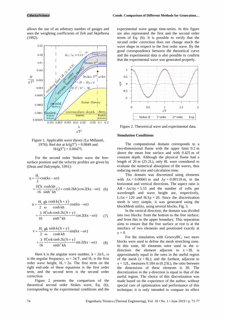
Figure 2 presents the comparison of the theoretical second order Stokes wave, Eq. (6), corresponding to the experimental conditions and the

experimental wave gauge time-series. In this figure are also represented the first and the second order terms of Eq. (6). It is possible to verify that the second order correction does not change much the wave shape in respect to the first order wave. By the good correspondence between the theoretical curve and the experimental data is also possible to confirm that the experimental wave was generated properly.

0 0.5 1 1.5 2t/T

-1

-0.5

0

0.5

1

η/a

Stokes II 1st order 2nd order Exp.

Figure 2. Theoretical wave and experimental data.

Simulation Conditions The computational domain corresponds to a

two-dimensional flume with the upper limit 0.2 m above the mean free surface and with 0.425 m of constant depth. Although the physical flume had a length of 20 m (25.2L), only 8L were considered to evaluate the numerical absorption of the waves, thus reducing mesh size and calculation time.

This domain was discretized using elements with ∆x = 0.00661 m and ∆y = 0.00119 m, in the horizontal and vertical directions. The aspect ratio is AR = ∆x/∆y = 5.55 and the number of cells per wavelength and wave height are, respectively, L/∆x = 120 and H/∆y = 20. Since the discretization mesh is very simple, it was generated using the blockMesh utility, using several blocks, Fig. 3.

In the vertical direction, the domain was divided into two blocks: from the bottom to the free surface; and from this to the upper boundary. This separation aims to ensure that the free surface at rest is at the interface of two elements and positioned exactly at y = 0.

For the simulation with GroovyBC, two more blocks were used to define the mesh stretching zone. In this zone, 60 elements were used in the x-direction: the element adjacent to x = 8L is approximately equal to the ones in the useful region of the mesh (x < 8L); and the furthest, adjacent to x = 12L, measures 0.184 m (0.23L), the ratio between the dimensions of these elements is 30. The discretization in the y-direction is equal to that of the useful region. The choice of this discretization was made based on the experience of the author, without special care of optimization and performance of this technique; it is only intended to compare its effect



with the result of the other solvers. The simulation conditions were chosen based on

the conclusions of Higuera et al. (2013) and Jacobsen et al. (2012). Many of the conditions of the baseWaveFlume examples (IHFoam/OlaFlow) and waveFlume (waves2Foam) were used in the present simulations. A maximum value of 0.25 was imposed for the Courant number.

a) waves2Foam

b) OlaFlow

c) GroovyBC

Figure 3. Domain characterization.

Although the wave is of the second order Stokes

type, a first order Stokes wave was generated. For the simulations with waves2Foam and IHFoam/OlaFlow the waves were generated by their generation routines, while for the GroovyBC utility the equations of the velocity components and volume fraction, for the linear wave theory, first terms of Eq. (6-8), were applied at the left border of the domain, Fig. 3. In this way, it is also possible to evaluate the wave transformation from first to second order along the flume. RESULTS AND DISCUSSION

Figure 4 shows the waterfall graphs for the three simulations performed. The vertical evolution is presented for 30 s of simulated time (t/T = 42), with a 0.1 s step and an amplification factor of 100 in the

wave height. It is clearly visible in these figures that there is reflection at the right end of the channel in the OlaFlow simulation; this behavior is due to the absorption method being derived from the shallow water theory, so it does not have the capacity to fully absorb the waves in deep water condition.

a) waves2Foam

b) OlaFlow

c) GroovyBC

Figure 4. Waterfall representation with amplification factor of 100 in the wave height.

y=0

y=0.2m

y=-0.425m

x=0

Mesh stretching zone Generation boundary

x=12L x=8L

y=0

y=0.2m

y=-0.425m

x=0

Absorption boundary Generation/absorption boundary

x=8L

y=0

y=0.2m

y=-0.425m

x=0 x=2L x=8L

Dissipation relaxation zone Generation relaxation zone

x=10L



For the waves2Foam simulation, the effect of the dissipation zone is visible for x > 8L, no reflection effect is visible since this zone has a 2L extension, enough to damp the waves (Jacobsen et al., 2012). For the GroovyBC simulation, the progressive effect of wave dissipation is visible for x > 8L and no reflection effect is visible.

Figure 4 provides qualitative information on the wave propagation and reflection in the domain but does not allow to accurately evaluate the waveform in time and space. As a complement to Fig. 4, the time evolution of the free surface for a probe placed at x/L = 4 is shown in Fig. 5. Figure 6 shows the free surface at instants, t/T, equal to 10, 25 and 40.

0 2 4 6 8 10 12 14 16 18 20 22 24 26 28 30t/T

-1

-0.5

0

0.5

1

η/a

x/L = 4

16 16.5 17t/T

-1

-0.5

0

0.5

1

η/a

OlaFlow

Stokes 2ndGroovyBCExp.

waves2Foam

40 41 42t/T

a)

b) c)

Figure 5. Wave gauge time series at x/L = 4. The simulated data results presented in Fig. 5

were time shifted to be is phase with the theoretical solution presented in Fig. 5b) for t/T = 16. It is observed that for x/L = 4: the waves2Foam solution is stable for t/T > 13; the OlaFlow solution shows reflection effects for t/T > 22; and the GroovyBC solution presents a progressive rise of the wave trough over time. For the last periods simulated, Fig. 5c), is also visible that all the simulations present a decrease of wave height: being smaller for waves2Foam and higher for GroovyBC; for OlaFlow the wave height decrease is partly due to the reflection. The waves2Foam solution doesn’t present any phase shift in the solution, OlaFlow solution present slight phase shift, and GroovyBC solution present the larger phase shift.

Figure 6 shows the free surface at instants, t/T, equal to 10, 25 and 40, without any imposed phase shift. The solutions are presented as they were

calculated, and it is verified that there is no temporal coincidence of the three simulations because the initial ramps are different in the three methods.

0 1 2 3 4 5 6 7 8 9 10 11 12x/L

-1

-0.5

0

0.5

1

/a

t/T = 25

0 1 2 3 4 5 6 7 8 9 10 11 12x/L

-1

-0.5

0

0.5

1

/a

t/T = 10

0 1 2 3 4 5 6 7 8 9 10 11 12x/L

-1

-0.5

0

0.5

1

/a

OlaFlow GroovyBC waves2Foam

t/T = 40

Figure 6. Free surface along the flume. Figure 6 shows that the waves2Foam solution is

stable at t/T = 25 for x/L > 3 and the wave is completely damped for x/L > 9. For t/T = 40 there is a slight decrease of the wave height in the flume relative to the previous instants. The OlaFlow solution shows reflection effects throughout the channel for t/T = 25 and 40. The GroovyBC solution presents an irregularly shaped solution for x/L > 8.5, which is a consequence of the progressively coarser mesh. There is a progressive rise of the wave troughs over time, visible in the three subfigures of Fig. 5, which is a consequence of the diffusive effect on the volume fraction, occurring in the dissipation zone, this effect is responsible for the decrease of the wave height and the mean water level rise over time. CONCLUSIONS

This paper presented the numerical simulations, using the OpenFOAM® software package, of non-breaking regular waves in a two-dimensional flume. A wave generation and absorption methods solution dependence studies were made for the waves2Foam and OlaFlow solvers and GroovyBC utility.

For the simulated wave characteristics, i.e.,



second order stokes in deep water condition, the OlaFlow solver does not have the ability to fully absorb the waves at the end of the flume, which is due to the absorption scheme being derived from the shallow water waves theory.

The waves2Foam solver showed good wave absorption capacity; however, there is a slight decrease in wave height along the flume. This behavior may possibly be improved by using a more refined mesh.

Using the GroovyBC utility to generate the waves proved to be adequate. The use of a progressively coarser mesh zone to absorb the waves, despite dissipating the waves, results in a mean water level rise in the flume over time, a decrease of wave height and a phase shift.

In conclusion, the waves2Foam solver proved to be more suitable for the simulations, since it does not introduce reflections in the flume, thus allowing simulations of longer duration with the same incident wave conditions. ACKNOWLEDGEMENTS

The author acknowledges the Research & Development Unit in Mechanical and Industrial Engineering (UNIDEMI) funding from the Portuguese Foundation for Science and Technology (FCT) UID/EMS/00667/2019. REFERENCES

Berberović, E., van Hinsberg, N. P., Jakirlić, S., Roisman, I. V., and Tropea, C., 2009, Drop Impact onto a Liquid Layer of Finite Thickness: Dynamics of the Cavity Evolution, Physical Review E, Vol. 79, No. 3, pp. 036306.

Beresford, P. J., 2003, HR Wavemaker Wave Generation Control Program - Software Manual, Report IT453, Issue5, HR Wallingford Limited.

Beresford, P. J., Spencer, J. M. A., and Clarke, J., 2005, HR Wavedata - Data Acquisition and Analysis Software - User Manual, HR Wallingford Limited.

Brackbill, J. U., Kothe, D. B., and Zemach, C., 1992, A Continuum Method for Modeling Surface Tension, Journal of Computational Physics, Vol. 100, No. 2, pp. 335-354.

Conde, J. M. P., Didier, E., Lopes, M. F. P., and Gato, L. M. C., 2009, Nonlinear Wave Diffraction by Submerged Horizontal Circular Cylinder, International Journal of Offshore and Polar Engineering, Vol. 19, No. 3, pp. 198-205.

Dean, R. G., and Dalrymple, R. A., 1991, Water Wave Mechanics for Engineers and Scientists, World Scientific.

Ferziger, J. H., and Peric, M., 2002, Computational Methods for Fluid Dynamics, 3rd Edition, Springer-Verlag Berlin Heidelberg.

Higuera, P., 2015, Application of

Computational Fluid Dynamics to Wave Action on Structures, PhD Thesis, University of Cantabria, Santander, Spain.

Higuera, P. C., Lara, J. L., and Losada, I. J., 2013, Realistic Wave Generation and Active Wave Absorption for Navier–Stokes Models: Application to OpenFOAM, Coastal Engineering, Vol. 71, pp. 102-118.

Hirt, C. W., and Nichols, B. D., 1981, Volume of Fluid (VOF) Method for the Dynamics of Free Boundaries, Journal of Computational Physics, Vol. 39, No. 1, pp. 201-225.

HR Wallingford, 2006, Wave Probe Monitor – User Manual, HR Wallingford Limited.

Isaacson, M., 1991, Measurement of Regular Wave Reflection, Journal of Waterway, Port, Coastal and Ocean Engineering, Vol. 117, No. 6, pp. 553-569.

Jacobsen, N. G., Fuhrman, D. R., and Fredsøe, J., 2012, A Wave Generation Toolbox for the Open-Source CFD Library: OpenFoam®, International Journal of Numerical Methods in Fluids, Vol. 70, pp. 1073-1088.

Jasak, H., 1996, Error Analysis and Estimation for the Finite Volume Method with Applications to Fluid Flows, PhD Thesis, Imperial College of Science, Technology and Medicine, London.

Le Méhauté, B., 1976, An Introduction to Hydrodynamics and Water Waves, Springer Berlin Heidelberg.

Mansard, E. P. D., and Funke, E. R., 1980, The Measurement of Incident and Reflected Spectra Using a Least Squares Method, in: 17th ICCE, Sydney, pp. 154-172.

Monaghan, J. J., 1992, Smoothed Particle Hydrodynamics, Annual Review of Astronomy and Astrophysics, Vol. 30, pp. 543-74.

OpenCFD, 2018, OpenFOAM - The Open Source CFD Toolbox - User Guide, OpenCFD Limited.

Rusche, H., 2002, Computational Fluid Dynamics of Dispersed Two-Phase Flows at High Phase Fractions, PhD Thesis, Imperial College of Science, Technology and Medicine, London.

Weller, H., Tabor, G., Jasak, H., and Fureby, C., 1998, A Tensorial Approach to Computational Continuum Mechanics Using Object-Oriented Techniques, Computers in Physics, Vol. 12, pp. 620-631.

Zelt, J. A., and Skjelbreia, J. E., 1992, Estimating Incident and Reflected Wave Fields Using an Arbitrary Number of Wave Gauges, in: 23rd ICCE, Venice, pp. 777-788.

Zienkiewicz, O. C., and Taylor, R. L., 2000, The Finite Element Method, Fluid Dynamics (Vol. 3), 3rd Edition, Butterworth-Heinemann.

COMPARISON OF DIFFERENT METHODS FOR GENERATION AND ...

Documents

Transcript of COMPARISON OF DIFFERENT METHODS FOR GENERATION AND ...