Comparison of different approaches for modeling of ... Code TAU of DLR Grid strategy...
53
Comparison of different approaches for modeling of atmospheric effects like gusts and wake-vortices in the CFD Code TAU Ralf Heinrich, Lars Reimer DLR Institute of Aerodynamics and Flow Technology International Forum on Aeroelasticity & Structural Dynamics 2017 Como, 25.06.-28.06.2017
Transcript of Comparison of different approaches for modeling of ... Code TAU of DLR Grid strategy...

Comparison of different approaches for modeling of atmospheric effects like gusts and wake-vortices in the CFD Code TAU
Ralf Heinrich, Lars ReimerDLR Institute of Aerodynamics and Flow Technology
International Forum on Aeroelasticity & Structural Dynamics 2017Como, 25.06.-28.06.2017

Comparison of different approaches for modeling of atmospheric effects in the CFD Code TAU
Overview Motivation CFD code TAU of DLR Methods for modeling of
atmospheric effects in TAU „Highly accurate“ method:
Resolved Atmosphere Approach (RAA)
Simplified method: Disturb-ance Velocity Approach (DVA)
Comparison of DVA and RAA Gust encounter Wake vortex encounter
Application Summary and outlook
wake vortex encounter of transport aircraft

Motivation
Hamburg, 3rd of March 2008, amateur videostrong winter storm “Emma”

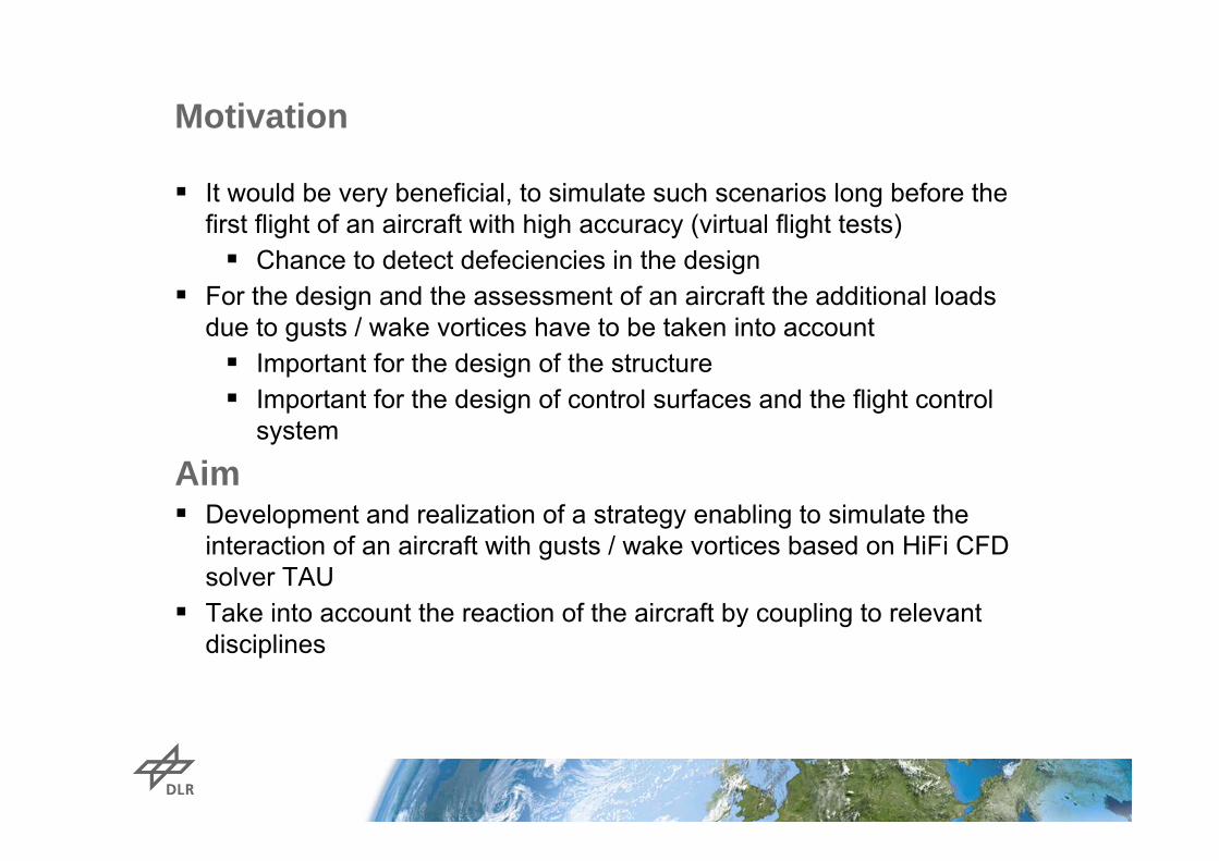
Motivation
It would be very beneficial, to simulate such scenarios long before the first flight of an aircraft with high accuracy (virtual flight tests) Chance to detect defeciencies in the design
For the design and the assessment of an aircraft the additional loads due to gusts / wake vortices have to be taken into account Important for the design of the structure Important for the design of control surfaces and the flight control
system
Aim Development and realization of a strategy enabling to simulate the
interaction of an aircraft with gusts / wake vortices based on HiFi CFD solver TAU
Take into account the reaction of the aircraft by coupling to relevant disciplines

CFD Code TAU of DLRGrid strategy unstructured/hybrid grids overset grids (Chimera) deforming grids grid adaptation (refinement, de-
refinement)Physical model 3D compressible Navier-Stokes
equations state-of-the-art turbulence models arbitrarily moving bodies steady and time accurate flowsNumerical algorithms 2nd order finite volume discretization
based on dual grid approach central and upwind schemes multigrid based on agglomeration Runge-Kutta or LU-SGS scheme implicit schemes for time accurate flows
(dual time stepping) MPI parallelization

CFD Code TAUGrid strategy unstructured/hybrid grids overset grids (Chimera) deforming grids grid adaptation (refinement, de-
refinement)Physical model 3D compressible Navier-Stokes
equations state-of-the-art turbulence models arbitrarily moving bodies steady and time accurate flowsNumerical algorithms 2nd order finite volume discretization
based on dual grid approach central and upwind schemes multigrid based on agglomeration Runge-Kutta or LU-SGS scheme implicit schemes for time accurate flows
(dual time stepping) MPI parallelization
Chimera technique with automatic hole cutting for simulation of moving spoilers

CFD Code TAUGrid strategy unstructured/hybrid grids overset grids (Chimera) deforming grids grid adaptation (refinement, de-
refinement)Physical model 3D compressible Navier-Stokes
equations state-of-the-art turbulence models arbitrarily moving bodies steady and time accurate flowsNumerical algorithms 2nd order finite volume discretization
based on dual grid approach central and upwind schemes multigrid based on agglomeration Runge-Kutta or LU-SGS scheme implicit schemes for time accurate flows
(dual time stepping) MPI parallelization
Mesh deformation for modeling of movables

CFD Code TAUGrid strategy unstructured/hybrid grids overset grids (Chimera) deforming grids grid adaptation (refinement, de-
refinement)Physical model 3D compressible Navier-Stokes
equations state-of-the-art turbulence models arbitrarily moving bodies steady and time accurate flowsNumerical algorithms 2nd order finite volume discretization
based on dual grid approach central and upwind schemes multigrid based on agglomeration Runge-Kutta or LU-SGS scheme implicit schemes for time accurate
flows (dual time stepping) MPI parallelization ),'('),'(')('' trvtrvtvv flexrottransB
dVv
SdTSdvvvdVvdtd
tV
tV tStSB
)(
)( )()(
''
''')''('''

Implementation of an unsteady boundary condition, to feed the atmospheric disturbances into the discretized flow domain
Methods for modeling of atmospheric effects in TAUResolved Atmosphere Approach (RAA)
Discretized flowfield
Additional inflow velocity prescribed at the boundary
t=t0

Implementation of an unsteady boundary condition, to feed the atmospheric disturbances into the discretized flow domain
Methods for modeling of atmospheric effects in TAUResolved Atmosphere Approach (RAA)
Discretized flowfield
t=t1

Implementation of an unsteady boundary condition, to feed the atmospheric disturbances into the discretized flow domain
Methods for modeling of atmospheric effects in TAUResolved Atmosphere Approach (RAA)
Discretized flowfield
t=t2

Implementation of an unsteady boundary condition, to feed the atmospheric disturbances into the discretized flow domain
Methods for modeling of atmospheric effects in TAUResolved Atmosphere Approach (RAA)
Discretized flowfield
t=t3

Implementation of an unsteady boundary condition, to feed the atmospheric disturbances into the discretized flow domain
Methods for modeling of atmospheric effects in TAUResolved Atmosphere Approach (RAA)
Discretized flowfield
t=t3
Advantage: Allows to capture mutual
interaction of atmospheric disturbance and aircraft
Disadvantage A high spatial resolution of
the COMPLETE flowfieldis required, to transport e.g. gusts without significant numerical losses
Very expensive . . . do exist alternatives??

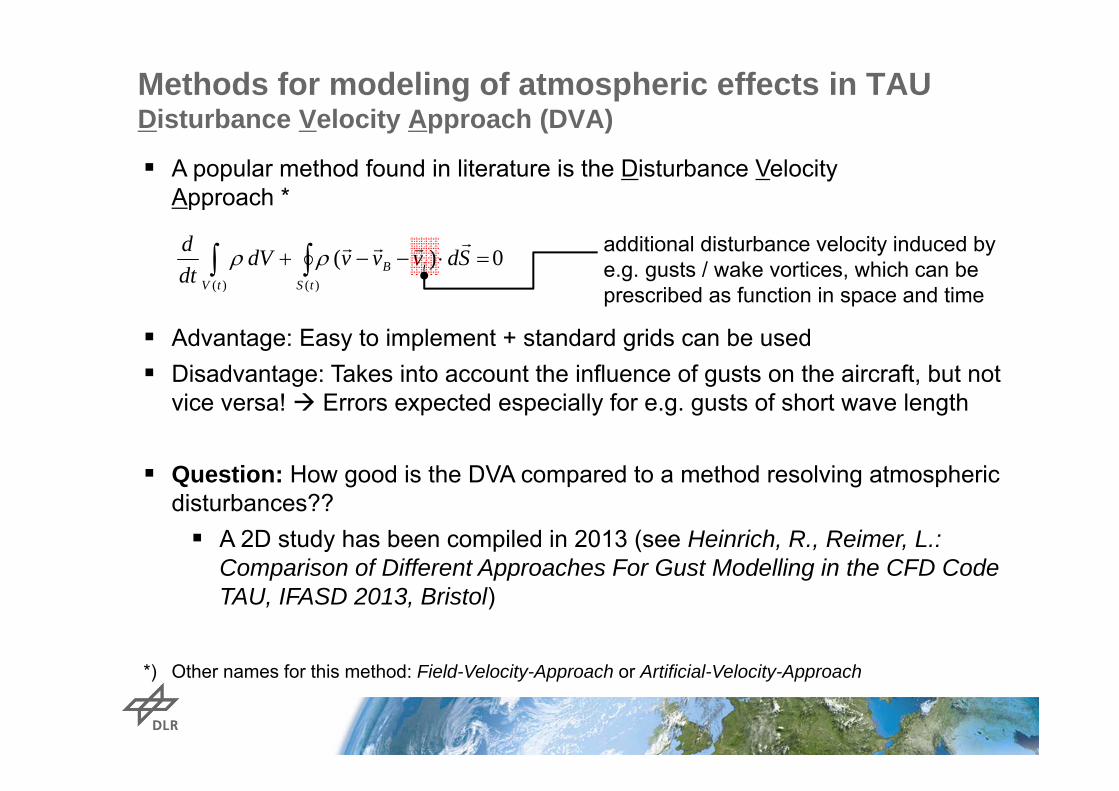
A popular method found in literature is the Disturbance Velocity Approach*
Methods for modeling of atmospheric effects in TAUDisturbance Velocity Approach (DVA)
*) Other names for this method: Field-Velocity-Approach or Artificial-Velocity-Approach
)( )(
0)(tV tS
iB SdvvvdVdtd additional disturbance velocity induced by
e.g. gusts / wake vortices, which can be prescribed as function in space and time
vi / vgust

A popular method found in literature is the Disturbance Velocity Approach *
Methods for modeling of atmospheric effects in TAUDisturbance Velocity Approach (DVA)
*) Other names for this method: Field-Velocity-Approach or Artificial-Velocity-Approach
)( )(
0)(tV tS
iB SdvvvdVdtd additional disturbance velocity induced by
e.g. gusts / wake vortices, which can be prescribed as function in space and time
vi / vgust
A popular method found in literature is the Disturbance Velocity Approach *
Methods for modeling of atmospheric effects in TAUDisturbance Velocity Approach (DVA)
)( )(
0)(tV tS
iB SdvvvdVdtd additional disturbance velocity induced by
e.g. gusts / wake vortices, which can be prescribed as function in space and time
Advantage: Easy to implement + standard grids can be used Disadvantage: Takes into account the influence of gusts on the aircraft, but not
vice versa! Errors expected especially for e.g. gusts of short wave length
Question: How good is the DVA compared to a method resolving atmosphericdisturbances?? A 2D study has been compiled in 2013 (see Heinrich, R., Reimer, L.:
Comparison of Different Approaches For Gust Modelling in the CFD Code TAU, IFASD 2013, Bristol)
*) Other names for this method: Field-Velocity-Approach or Artificial-Velocity-Approach

t / tref
lift
15 20 25 30 35 400
0.1
0.2
0.3
/cref = 2
Ma = 0.25, NSRGA: solid lineDVA: dashed line
Ma = 0.25, Re = 5 x 10⁶
Solid : RAADashed : DVA
gust / cref
Results of 2D study NACA wing-HTP configuration Ma = 0.25; Ma = 0.75 Viscous and inviscid / cref = 1, 2, 4
%100max,,
max,,max,,max,
RGAL
DVALRGALC c
ccerr
L
Methods for modeling of atmospheric effects in TAUComparison of DVA and RAA for gusts
/ cref errCL,max [%]
Ma = 0,25 Ma = 0,75 Euler NS Euler NS
1 1,96 2,16 10,69 11,082 1,16 1,24 2,72 2,934 0,21 0,47 0,42 0,64
RAA & DVA results are very similar for gust / cref ≥ 2 (for vertical gusts in 2D)!

Extend study to 3D Usage of configuration with
forward swept wing Ma = 0.78 Re = 26.4 x 106
= 0.0° gust / cref= 1, 2, 4 vgust / vinf = 0.1 Altitude h = 11 km Basic grid: 11.2 x 10⁶ nodes
Methods for modeling of atmospheric effects in TAUComparison of DVA and RAA for gusts

Extend study to 3D Usage of configuration with
forward swept wing Ma = 0.78 Re = 26.4 x 106
= 0.0° gust / cref= 1, 2, 4 vgust / vinf = 0.1 Altitude h = 11 km Basic grid: 11.2 x 10⁶ nodes Create nearfield grid based on
basic grid
Methods for modeling of atmospheric effects in TAUComparison of DVA and RAA for gusts

Extend study to 3D Usage of configuration with
forward swept wing Ma = 0.78 Re = 26.4 x 106
= 0.0° gust / cref= 1, 2, 4 vgust / vinf = 0.1 Altitude h = 11 km Basic grid: 11.2 x 10⁶ nodes Create nearfield grid based on
basic grid Embed this into a Cartesian
background mesh
Methods for modeling of atmospheric effects in TAUComparison of DVA and RAA for gusts
x = 0.05 cref

Extend study to 3D Usage of configuration with
forward swept wing Ma = 0.78 Re = 26.4 x 106
= 0.0° gust / cref= 1, 2, 4 vgust / vinf = 0.1 Altitude h = 11 km Basic grid: 11.2 x 10⁶ nodes Create nearfield grid based on
basic grid Embed this into a Cartesian
background mesh Add fine resolved gust
transport mesh In total 17.3 x 10⁶ nodes
Methods for modeling of atmospheric effects in TAUComparison of DVA and RAA for gusts
x = 0.01 gustx = 0.05 cref
t = 0; gust in front of flow domain

Extend study to 3D Usage of configuration with
forward swept wing Ma = 0.78 Re = 26.4 x 106
= 0.0° gust / cref= 1, 2, 4 vgust / vinf = 0.1 Altitude h = 11 km Basic grid: 11.2 x 10⁶ nodes Create nearfield grid based on
basic grid Embed this into a Cartesian
background mesh Add fine resolved gust
transport mesh In total 17.3 x 10⁶ nodes
Methods for modeling of atmospheric effects in TAUComparison of DVA and RAA for gusts
x = 0.01 gustx = 0.05 cref
t = 1.5 gust/uinf; gust centered in transport grid

Extend study to 3D Usage of configuration with
forward swept wing Ma = 0.78 Re = 26.4 x 106
= 0.0° gust / cref= 1, 2, 4 vgust / vinf = 0.1 Altitude h = 11 km Basic grid: 11.2 x 10⁶ nodes Create nearfield grid based on
basic grid Embed this into a Cartesian
background mesh Add fine resolved gust
transport mesh In total 17.3 x 10⁶ nodes
Methods for modeling of atmospheric effects in TAUComparison of DVA and RAA for gusts
x = 0.01 gustx = 0.05 cref
transport grid is moving with uinf
uinf

t [s]
C-li
ft
0.2 0.3 0.4 0.5 0.6
0.5
0.55
0.6
0.65
0.7
0.75
0.8
RGADVA
Solid:Dashed:
gust / cref = 4
gust / cref = 1gust / cref = 2
Results of 3D study Ma = 0.78 Re = 26.4 x 106
= 0.0° gust / cref= 1, 2, 4 vgust / vinf = 0.1 Altitude h = 11 km
Methods for modeling of atmospheric effects in TAUComparison of DVA and RAA for gusts
/ cref errCL,max
1 1.42% 2 1.28% 4 0.42%
Solid: RAADashed: DVA
%100max,,
max,,max,,max,
RAAL
DVALRAALC c
ccerr
L

t [s]
C-li
ft
0.2 0.3 0.4 0.5 0.6
0.5
0.55
0.6
0.65
0.7
0.75
0.8
RGADVA
Solid:Dashed:
gust / cref = 4
gust / cref = 1gust / cref = 2
Results of 3D study Ma = 0.78 Re = 26.4 x 106
= 0.0° gust / cref= 1, 2, 4 vgust / vinf = 0.1 Altitude h = 11 km
Methods for modeling of atmospheric effects in TAUComparison of DVA and RAA for gusts
/ cref errCL,max
1 1.42% 2 1.28% 4 0.42%
Solid: RAADashed: DVA
3D results show similar trends compared to 2D simulations.
DVA is sufficient accurate for gust load prediction down to gust / cref = 2

0
0 y
Vt(r)
vortex core with radius rc
distance b
r2
Vt,2
r1
Vt,1
Methods for modeling of atmospheric effects in TAUComparison of DVA and RAA for wake vortex encounter problems
DVA and RAA can now also be applied for simulation of wake vortex encounters Analytical function according to
Burnham-Hallock
Disturbance velocity field is created by superposition of two counter rotating vortices with circulation and distance b
222 rrrrV
ct
Methods for modeling of atmospheric effects in TAUComparison of DVA and RAA for wake vortex encounter problems
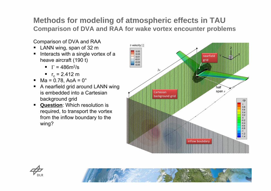
Comparison of DVA and RAA LANN wing, span of 32 m Interacts with a single vortex of a
heave aircraft (190 t) = 486m2/s rc = 2.412 m
Ma = 0.78, AoA = 0° A nearfield grid around LANN wing
is embedded into a Cartesian background grid
Question: Which resolution is required, to transport the vortex from the inflow boundary to the wing?

Methods for modeling of atmospheric effects in TAUComparison of DVA and RAA for wake vortex encounter problems
Comparison of DVA and RAA LANN wing, span of 32 m Interacts with a single vortex of a
heave aircraft (190 t) = 486m2/s rc = 2.412 m
Ma = 0.78, AoA = 0° A nearfield grid around LANN wing
is embedded into a Cartesian background grid
Question: Which resolution is required, to transport the vortex from the inflow boundary to the wing? Perform a mesh density study
10 cells to resolve rc
5 cells to resolve rc
2.5 cells to resolve rc

Methods for modeling of atmospheric effects in TAUComparison of DVA and RAA for wake vortex encounter problems
Results of mesh conversion study

Methods for modeling of atmospheric effects in TAUComparison of DVA and RAA for wake vortex encounter problems
Results of mesh conversion study (results on a ray through the vortex core)

Methods for modeling of atmospheric effects in TAUComparison of DVA and RAA for wake vortex encounter problems
Results of mesh conversion study (results on a ray through the vortex core)
To be on the safe side, the fine resolution has been selected for the computation of wake vortex encounter of the LANN wing
N
i in
iinioutmean w
wwN
err1 max,
,, %100*1 %100*maxmax,
,,max
in
iiniout
www
err
Fine mesh Medium mesh Coarse mesh errmax 0.90% 4.95% 15.88% errmean 0.11% 0.64% 2.57%

Methods for modeling of atmospheric effects in TAUComparison of DVA and RAA for wake vortex encounter problems
Comparison of DVA and RAA LANN wing, span of 32 m Interacts with a single
vortex of a heave aircraft (190 t) = 486m2/s rc = 2.412 m
Ma = 0.78, AoA = 0° Nearfield grid around
LANN with 4.8 x 10⁶ nodes Cartesian background
mesh with 2.8 x 10⁶ nodes

Methods for modeling of atmospheric effects in TAUComparison of DVA and RAA for wake vortex encounter problems
Comparison of DVA and RAA LANN wing, span of 32 m Interacts with a single
vortex of a heave aircraft (190 t) = 486m2/s rc = 2.412 m
Ma = 0.78, AoA = 0° Variation of core position
from tip to tip
+cmx
DVARAADVARAA

Methods for modeling of atmospheric effects in TAUComparison of DVA and RAA for wake vortex encounter problems
Comparison of DVA and RAA LANN wing, span of 32 m Interacts with a single
vortex of a heave aircraft (190 t) = 486m2/s rc = 2.412 m
Ma = 0.78, AoA = 0° Variation of core position
from tip to tip The prediction error of lift
and rolling moment coeff. is below 1%!
%100*min,,max,,
,,,,,
RAALRAAL
RAAiLDVAiLiCL CC
CCerr
DVA is well suited for wake vortex encounter studies

ApplicationWake vortex encounter of transport aircraft
Transport aircraft (70 t) flying through wake vortices of heavy aircraft (190 t)
Ma = 0.78, h = 37.000 ft Usage of DVA for modeling of
wake of leading aircraft = 486m2/s rc = 2.412 m b = 47.36 m
Perform unsteady CFD simulation (guided motion)
Perform unsteady coupled simulation (CFD-FM)
Aircraft is in the plain of the vortex pair
= 5°initial situation
mid of simulation
Transport aircraft is 5 m beneath vortex pair
mid of simulation,slice through the disturbance velocity field
Transport aircraft Transport aircraft

ApplicationWake vortex encounter of transport aircraft

ApplicationWake vortex encounter of transport aircraft

ApplicationWake vortex encounter of transport aircraft

ApplicationWake vortex encounter of transport aircraft

ApplicationWake vortex encounter of transport aircraft

ApplicationWake vortex encounter of transport aircraft

ApplicationWake vortex encounter of transport aircraft

.
Transport aircraft (70 t) flying through wake vortices of heavy aircraft (190 t)
Ma = 0.78, h = 37.000 ft Usage of DVA* for modeling of
wake of leading aircraft = 486m2/s rc = 2.412 m b = 47.36
Perform unsteady CFD simulation (guided motion)
Perform unsteady coupled simulation (CFD-FM)
ApplicationWake vortex encounter of transport aircraft
time [s]
C-li
ft
2 4 6 8
0.4
0.5
0.6
0.7
0.8 CFDCFD-FM
Comparison of monodisciplinary and multidisciplinary simulation
*) Disturbance Velocity Approach

Summary
Two methods for modeling of atmospheric disturbances are available in TAU now: Simplified approach: DVA A „highly-accurate“ method allowing to simulate the mutual
interaction of aircraft and atmospheric disturbances: RAA Comparison of both methods in terms of global loads show that: DVA achieves results comparable to results of „highly-accurate“
method down to gust / cref ≥ 2.0 for viscous and inviscid flow in 2D and 3D for vertical gusts
Very good agreement of DVA and RAA for gust encounter problems

Next steps
Perform similar investigation for lateral gusts Maybe the interaction of the lateral gust with the tip vortices have a
significant impact on the results, which cannot be captured by the DVA
Acknowledgement
The research leading to these results has partly been supported by the AEROGUST project funded by the European Commission under grant agreement number 636053 and the German research project FOR1066“Simulation des Überziehen von Tragflügeln und Triebwerksgondeln” funded by the “Deutsche Forschungsgemeinschaft DFG”

Thank you for your attention!
sea level