HAL Id: hal-00683233https://hal.archives-ouvertes.fr/hal-00683233

Submitted on 28 Mar 2012

HAL is a multi-disciplinary open accessarchive for the deposit and dissemination of sci-entific research documents, whether they are pub-lished or not. The documents may come fromteaching and research institutions in France orabroad, or from public or private research centers.

L’archive ouverte pluridisciplinaire HAL, estdestinée au dépôt et à la diffusion de documentsscientifiques de niveau recherche, publiés ou non,émanant des établissements d’enseignement et derecherche français ou étrangers, des laboratoirespublics ou privés.

Comparison of color demosaicing methodsOlivier Losson, Ludovic Macaire, Yanqin Yang

To cite this version:Olivier Losson, Ludovic Macaire, Yanqin Yang. Comparison of color demosaicing methods. Advancesin Imaging and Electron Physics, Elsevier, 2010, 162, pp.173-265. �10.1016/S1076-5670(10)62005-8�.�hal-00683233�

Comparison of color demosaicing methods

O. Lossona,∗, L. Macairea, Y. Yanga

a Laboratoire LAGIS UMR CNRS 8146 – Bâtiment P2Université Lille1 – Sciences et Technologies, 59655 Villeneuve d’Ascq Cedex, France

Keywords: Demosaicing, Color image, Quality evaluation, Comparisoncriteria

1. Introduction

Today, the majority of color cameras are equipped with a single CCD (Charge-Coupled Device) sensor. The surface of such a sensor is covered by a color filter array(CFA), which consists in a mosaic of spectrally selective filters, so that each CCD ele-ment samples only one of the three color components Red (R), Green (G) or Blue (B).The Bayer CFA is the most widely used one to provide the CFA image where each pixelis characterized by only one single color component. To estimate the color (R,G,B) ofeach pixel in a true color image, one has to determine the values of the two missing co-lor components at each pixel in the CFA image. This process iscommonly referred toas CFA demosaicing, and its result as the demosaiced image. In this paper, we proposeto compare the performances reached by the demosaicing methods thanks to specificquality criteria.

An introduction to the demosaicing issue is given in section2. Besides explainingwhy this process is required, we propose a general formalismfor it. Then, two ba-sic schemes are presented, from which are derived the main principles that should befulfilled in demosaicing.

In section3, we detail the recently published demosaicing schemes which are re-grouped into two main groups : the spatial methods which analyze the image planeand the methods which examines the frequency domain. The spatial methods exploitassumptions about either spatial or spectral correlation between colors of neighbors.The frequency-selection methods apply specific filters on the CFA image to retrievethe color image.

Since these methods intend to produce “perceptually satisfying” demosaiced images,the most widely used evaluation criteria detailed in section 4 are based on the fidelityto the original images. Generally, the Mean Square Error (MSE) and the Peak Signal-to-Noise Ratio (PSNR) are used to measure the fidelity between the demosaiced imageand the original one. ThePSNRcriterion cannot distinguish the case when there are

∗Corresponding authorEmail addresses:olivier.losson@univ-lille1.fr (O. Losson),

ludovic.macaire@univ-lille1.fr (L. Macaire),yanqin.yang@etudiant.univ-lille1.fr (Y. Yang)

Preprint submitted to Advances in imaging and electron physics 18 décembre 2009

a high number of pixels with slight estimation errors from the case when only a fewpixels have been interpolated with severe demosaicing artifacts. However, the lattercase would more significantly affect the result quality of a low-level analysis appliedto the estimated image. Therefore, we propose new criteria especially designed to de-termine the most effective demosaicing method for further feature extraction.

The performances of the demosaicing methods are compared insection5 thanks tothe presented measurements. For this purpose, the demosaicing schemes are applied totwelve images of the benchmark Kodak database.

2

2. Color Demosaicing

Digital images or videos are currently a preeminent medium in environment per-ception. They are today almost always captured directly by adigital (still) camera,rather than digitized from a video signal provided by an analog camera as they used tobe several years ago. Acquisition techniques ofcolor images in particular have invol-ved much research work and undergone many changes. Despite major advancements,mass-market color cameras still often use a single sensor and require subsequent pro-cessing to deliver color images. This procedure, nameddemosaicing, is the key pointof our study and is introduced in the present section. The demosaicing issue is firstpresented in detail, and a formalism is introduced for it.

2.1. Introduction to the Demosaicing Issue

The demosaicing issue is here introduced from technological considerations. Twomain types of color digital cameras are found on the market, depending on whether theyembed three sensors or a single one. Usually known asmono-CCDcameras, the latterare equipped with spectrally-sensitive filters arranged according to a particular pattern.From such color filter arrays (CFA), an intermediate gray-scale image is formed, whichthen has to bedemosaicedinto a true color image.

In the first subsection are compared the major implementations of three-CCD andmono-CCD technologies. Then are presented the main types ofcolors filter arrays re-leased by the various manufacturers. Proposed by Bayer fromKodak in 1976, the mostwidespread CFA is considered in the following, not only to formalize demosaicing butalso to introduce a pioneer method using bilinear interpolation. This basic scheme ge-nerates many color artifacts, which are analyzed to derive two main demosaicing rules.Spectral correlation is one of them, and will be detailed in the last subsection. Thesecond one, spatial correlation, is at the heart of edge-adaptive demosaicing methods,that will be presented in the next section.

2.1.1. Mono-CCD vs. Three-CCD Color CamerasDigital area scan cameras are devices able to convert color stimuli from the ob-

served scene into a color digital image (or image sequence) thanks to photosensors.Such an output image is spatially digitized, being formed ofpicture elements (pixels).With each pixel is generally associated a single photosensor element, which capturesthe incident light intensity of the color stimulus.

A digital color imageI can be represented as a matrix of pixels, each of them beingdenoted asP(x,y), wherex andy are the spatial coordinates of pixelP within the imageplane of sizeX ×Y, hence(x,y) ∈ N

2 and 06 x 6 X −1, 06 y 6 Y−1. With eachpixel P is associated a color point, denoted asI(x,y) or Ix,y. This color point is definedin the RGB three-dimensional color space by its three coordinatesIk

x,y, k ∈ {R,G,B},which represent the levels of the trichromatic components of the corresponding colorstimulus.

The color imageI may also be split into threecomponent planesor images Ik,k ∈ {R,G,B}. In each component imageIk, the pixelP is characterized by levelIk(P)for the single color componentk. Thus, three component imagesIR, IG andIB, must beacquired in order to form any digital color image.

3

R

G

B

stimulus

dichroicprism

CCDsensor

(a) Beam splitting by a trichroic prism assembly.

350 400 450 500 550 600 650 700 750 800 8500

10

20

30

40

50

60

70

80

90

100

Wavelengthλ (nm)

Sp

ect

rals

en

sitiv

ity

R(λ )

G(λ )B(λ )

(b) Relative spectral sensitivity of the Kodak KLI-2113 sensor.

380 420 460 500 540 580 620 660 700 740 780

0.40

−0.10

0.35

0.30

0.25

0.20

0.15

0.10

0.05

0

−0.05

Wavelengthλ (nm)

Sp

ect

rals

en

sitiv

ity

Rc(λ )

Gc(λ )

Bc(λ )

[Rc][Gc][Bc]

(c) CIE 1931 RGB color matching functions.[Rc],[Gc] and[Bc] are the monochromatic primary colors.

FIG. 1: Three-CCD technology.

The two main technology families available for the design ofdigital camera photo-sensors are CCD (Charge-Coupled Device) and CMOS (Complementary Metal-OxideSemiconductor) technologies, the former being the most widespread one today. TheCCD technology uses the photoelectric effect of the siliconsubstrate, while CMOS isbased on a photodetector and an active amplifier. Both photosensors overall convertthe intensity of the light reaching each pixel into a proportional voltage. Additionalcircuits then converts this analog voltage signal into digital data. For illustration andexplanation purposes, the following text relates to the CCDtechnology.

The various digital color cameras available on the market may also be distingui-shed according to whether they incorporate only a single sensor or three. In accordancewith the trichromatic theory, three-CCD technology incorporates three CCD sensors,each one being dedicated to a specific primary color. In most devices, the color sti-mulus from the observed scene is split onto the three sensorsby means of a trichroic

4

RGBB

stimulus

CMOSsensor

(a) Wavelength absorption within the Foveon X3 sensor.

0.045

700650600550500450400350

0

0.040

0.035

0.030

0.025

0.020

0.015

0.010

0.005

Sp

ect

rals

en

sitiv

ity

Wavelengthλ (nm)

R(λ )

G(λ )B(λ )

(b) Relative spectral sensitivity of the Foveon X3 sensor endowed with an infraredfilter (Lyon and Hubel, 2002).

FIG. 2: Foveon X3 technology.

prism assembly, made of two dichroic prisms (see figure1a)(Lyon, 2000). Alternately,the incident beam may be dispatched on three sensors, each one being covered witha spectrally selective filter. The three component imagesIR, IG and IB are simulta-neously acquired by the three CCD sensors, and their combination leads to the finalcolor image. Each digital three-CCD camera is characterized by its own spectral sensi-tivity functionsR(λ ), G(λ ) andB(λ ) (see figure1bfor an example), which differ fromthe CIE color matching functions of the standard observer (see figure1b).

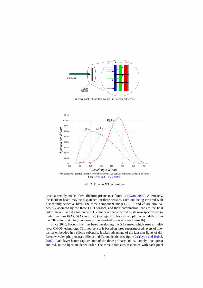
Since 2005, Foveon Inc. has been developing the X3 sensor, which uses a multi-layer CMOS technology. This new sensor is based on three superimposed layers of pho-tosites embedded in a silicon substrate. It takes advantageof the fact that lights of dif-ferent wavelengths penetrate silicon to different depths (see figure2a)(Lyon and Hubel,2002). Each layer hence captures one of the three primary colors,namely blue, greenand red, in the light incidence order. The three photosites associated with each pixel

5

thus provide signals from which the three component values are derived. Any cameraequipped with this sensor is able to form a true color image from three full componentimages, as do three-CCD-based cameras. This sensor has beenfirst used commerciallyin 2007 within the Sigma SD14 digital still camera. According to its manufacturer, itsspectral sensitivity (see figure2b) better fits with the CIE color matching functionsthan those of three-CCD cameras, providing images that are more consistent with hu-man perception.

Although three-CCD and Foveon technologies yield high quality images, the manu-facturing costs of the sensor itself and of the optical device are high. As a consequence,cameras equipped with such sensors have not been so far affordable to everyone, norwidely distributed.

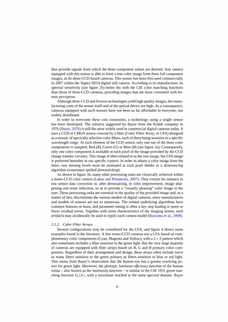
In order to overcome these cost constraints, a technology using a single sensorhas been developed. The solution suggested by Bayer from theKodak company in1976 (Bayer, 1976) is still the most widely used in commercial digital camerastoday. Ituses a CCD or CMOS sensor covered by a filter (Color Filter Array, or CFA) designedas a mosaic of spectrally selective color filters, each of them being sensitive to a specificwavelength range. At each element of the CCD sensor, only oneout of the three colorcomponents is sampled, Red (R), Green (G) or Blue (B) (see figure3a). Consequently,only one color component is available at each pixel of the image provided by the CCDcharge transfer circuitry. This image if often related to astheraw image, butCFA imageis preferred hereafter in our specific context. In order to obtain a color image from thelatter, two missing levels must be estimated at each pixel thanks to ademosaicingalgorithm (sometimes spelleddemosaicking).

As shown in figure3b, many other processing tasks are classically achieved withina mono-CCD color camera (Lukac and Plataniotis, 2007). They consist for instance inraw sensor data correction or, after demosaicing, in color improvement, image shar-pening and noise reduction, so as to provide a “visually pleasing” color image to theuser. These processing tasks are essential to the quality ofthe provided image and, as amatter of fact, discriminate the various models of digital cameras, since manufacturersand models of sensors are not so numerous. The related underlying algorithms havecommon features or basis, and parameter tuning is often a keystep leading to more orfewer residual errors. Together with noise characteristics of the imaging sensor, suchartifactsmay incidentally be used to typify each camera model (Bayrama et al., 2008).

2.1.2. Color Filter ArraysSeveral configurations may be considered for the CFA, and figure 4 shows some

examples found in the literature. A few mono-CCD cameras usea CFA based on com-plementary color components (Cyan, Magenta and Yellow), with a 2×2 pattern whichalso sometimes includes a filter sensitive to the green light. But the very large majorityof cameras are equipped with filter arrays based onR, G andB primary color com-ponents. Regardless of their arrangement and design, thesearrays often include twiceas many filters sensitive to the green primary as filters sensitive to blue or red light.This stems from Bayer’s observation that the human eye has a greater resolving po-wer for green light. Moreover, the photopicluminous efficiency functionof the humanretina – also known as theluminosity function– is similar to the CIE 1931 green mat-ching functionGc(λ ), with a maximum reached in the same spectral domain. Bayer

6

CCD

G

R

B

GCFA

image

(Bayer)CFA

Color FilterArray (CFA)

stimulus

(a) Mono-CCD technology outline, using the Bayer Color Filter Array (CFA).

CFA image

CFAdata

pre-processing

defective pixelcorrection

linearizationdark current

compensationwhite

balance

image CFA

imageprocessing

digital zoom onthe CFA image

demosaicingestimated imagepost-processing

digital zoom onthe estimated image

post-processing

colorcorrection

sharpening andnoise reduction

estimatedcolor image

storage

imagecompression

EXIF fileformatting

(b) Image acquisition within a mono-CCD color camera (detailedschema). Dotted steps are optional.

FIG. 3: Internal structure of a mono-CCD color camera.

7

(a) Vertical stripes (b) Bayer (c) Pseudo-random

(d) Complementary colors (e) “Panchromatic”, orCFA2.0 (Kodak)

(f) “Burtoni” CFA

FIG. 4: Configuration examples for the mosaic of color filters. Each square depicts apixel in the CFA image, and its color is that of the monochromatic filter covering theassociated photosite.

therefore both makes the assumption that green photosensors capture luminance, whe-reas red and blue ones capture chrominance, and suggests to fill the CFA with moreluminance-sensitive (green) elements than chrominance-sensitive (red and blue) ele-ments (see figure4b).

The CFA using alternating vertical stripes (see figure4a) of the RGB primarieshas been released first, since it is well suited to the interlaced television video signal.Nevertheless, considering the Nyquist limits for the greencomponent plane,Parulski(1985) shows that the Bayer CFA has larger bandwidth than the latter for horizontalspatial frequencies. The pseudo-random filter array (see figure 4c) has been inspiredby the human eye physiology, in an attempt to reproduce the spatial repartition of thethree cone cell types on the retina surface (Lukac and Plataniotis, 2005a). Its irregula-rity achieves a compromise between the sensitivity to spatial variations of luminancein the observed scene (visual acuity) and the ability to perceive thin objects with dif-ferent colors (Roorda et al., 2001). Indeed, optimal visual acuity would require pho-tosensors with identical spectral sensitivities which areconstant over the spectrum,whereas the perception of thin color objects is better ensured with sufficient localdensity of different types of cones. Despite pseudo-randomcolor filter arrays showinteresting properties (Alleysson et al., 2008), their design and exploitation have notmuch been investigated so far ; for some discussions, see e.g. Condat(2009) or Savard(2007) about CFA design andZapryanov and Nikolova(2009) about demosaicing ofBayer CFA “pseudo-random” variations. Among other studiesdrawing their inspira-tion from natural physiology for CFA design, Kröger’s work (2004) yields a new mo-

8

0

700650600550500450400

0.2

0.4

0.6

0.8

1.0

Wavelengthλ (nm)

Sp

ect

rals

en

sitiv

ity

C(λ )

G(λ )

Y(λ )

M(λ )

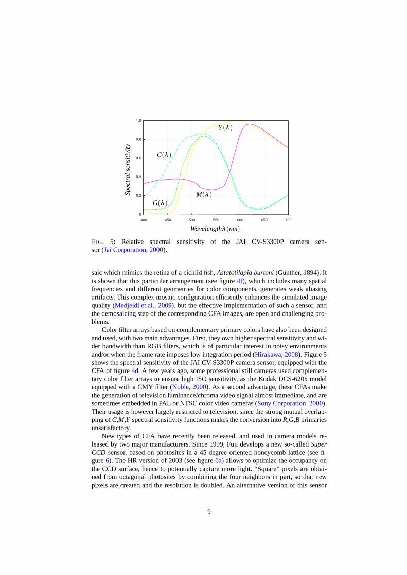
FIG. 5: Relative spectral sensitivity of the JAI CV-S3300P camera sen-sor (Jai Corporation, 2000).

saic which mimics the retina of a cichlid fish,Astatotilapia burtoni(Günther, 1894). Itis shown that this particular arrangement (see figure4f), which includes many spatialfrequencies and different geometries for color components, generates weak aliasingartifacts. This complex mosaic configuration efficiently enhances the simulated imagequality (Medjeldi et al., 2009), but the effective implementation of such a sensor, andthe demosaicing step of the corresponding CFA images, are open and challenging pro-blems.

Color filter arrays based on complementary primary colors have also been designedand used, with two main advantages. First, they own higher spectral sensitivity and wi-der bandwidth than RGB filters, which is of particular interest in noisy environmentsand/or when the frame rate imposes low integration period (Hirakawa, 2008). Figure5shows the spectral sensitivity of the JAI CV-S3300P camera sensor, equipped with theCFA of figure4d. A few years ago, some professional still cameras used complemen-tary color filter arrays to ensure high ISO sensitivity, as the Kodak DCS-620x modelequipped with a CMY filter (Noble, 2000). As a second advantage, these CFAs makethe generation of television luminance/chroma video signal almost immediate, and aresometimes embedded in PAL or NTSC color video cameras (Sony Corporation, 2000).Their usage is however largely restricted to television, since the strong mutual overlap-ping ofC,M,Y spectral sensitivity functions makes the conversion intoR,G,B primariesunsatisfactory.

New types of CFA have recently been released, and used in camera models re-leased by two major manufacturers. Since 1999, Fuji develops a new so-calledSuperCCD sensor, based on photosites in a 45-degree oriented honeycomb lattice (see fi-gure6). The HR version of 2003 (see figure6a) allows to optimize the occupancy onthe CCD surface, hence to potentially capture more light. “Square” pixels are obtai-ned from octagonal photosites by combining the four neighbors in part, so that newpixels are created and the resolution is doubled. An alternative version of this sensor

9

Created pixel

(a) Super CCD HR(2003)

“R pixel” “S pixel”Photosite

(b) Super CCD SR(2003)

“R pixel”“S pixel”

(c) Super CCD SRII(2004)

Coupled pixels

(d) Super CCD EXR(2008)

FIG. 6: Super CCD technology. For clarity sake, photosites are represented furtherapart from each other than at their actual location.

(SR, see figure6b) has expanded dynamic range, by incorporating both high-sensitivitylarge photodiodes (“S-pixels”) used to capture normal and dark details, and smaller “R-pixels” sensitive to bright details. The EXR version (see figure6d) takes advantage ofsame idea, but extra efforts have been conducted on noise reduction thanks to pixelbinning, resulting in a new CFA arrangement and its exploitation by pixel coupling. Asa proprietary technology, little technical detail is available on how Super CCD sensorsturn the image into an horizontal/vertical grid without interpolating, or on how demo-saicing associated with such sensors is achieved. A few hints may however be found ina patent using a similar imaging device (Kuno and Sugiura, 2006).

In 2007, Kodak develops new filter arrays (Hamilton and Compton, 2007) as ano-ther alternative to the widely used Bayer CFA. The basic principle of this so-calledCFA2.0 family of color filters is to incorporate transparentfilter elements (represen-ted as white squares on figure4e), those filters being hence also known asRGBWor“panchromatic” ones. This property makes the underlying photosites sensitive to allwavelengths of the visible light. As a whole, the sensors associated with CFA2.0 aretherefore more sensitive to low-energy stimuli than those using Bayer CFA. Such in-crease of global sensitivity leads to better luminance estimation, but at the expenseof chromatic information estimation. Figure7 shows the processing steps required toestimate a full color image from the data provided by a CFA2.0-based sensor.

By modifying the CFA arrangement, manufacturers primarilyaim at increasingthe spectral sensitivity of the sensor.Lukac and Plataniotis(2005a) tackled the CFAdesign issue by studying the influence of the CFA configuration on demosaicing results.They considered ten different RGB color filter arrays, threeof them being shown onfigures4a to 4c. A CFA image is first simulated by sampling one out of the threecolor components at each pixel in an original color image, according to the consideredCFA pattern. A universal demosaicing framework is then applied to obtain a full-colorimage. The quality of the demosaiced image is finally evaluated by comparing it to theoriginal image thanks to several objective error criteria.The authors conclude that theCFA design is critical to demosaicing quality results, but cannot advise any CFA thatwould yield best results in all cases. Indeed, the relative performance of filters is highlydependent on the tested image.

10

B B B B

B B B B

B B B B

B B B B

G G G G

G G G G

G G G G

G G G G

B−P B−P B−P B−P

B−P B−P B−P B−P

B−P B−P B−P B−P

B−P B−P B−P B−P

G−P G−P G−P G−P

G−P G−P G−P G−P

G−P G−P G−P G−P

G−P G−P G−P G−P

B B

B B

G G

G G

G

B G

B

G

G R

R

B G

G R

P P

P

P P

P

P P

interpolation

P P

P

P P

P

P P

P P

P P

P PP P

−interpolation

R−P R−P R−P R−P

R−P R−P R−P R−P

R−P R−P R−P R−P

R−P R−P R−P R−P

+

P P

PP

R R

R R

B−P B−P

B B−P

G−PG−P

G G−P

R−PR−P

R−P R−P

R R R R

R R R R

R R R R

R R R R

Color componentpixels

Panchromatic pixels

CFA image

(reduced resolution)

(reduced resolution)

(reduced resolution)

(reduced resolution)

(full resolution)

(full resolution)

(full resolution)

Chrominance-luminance

Chrominance-luminance

image

image

Color image

Color image

Luminance image

Luminance image

averaging

averaging demosaicing

FIG. 7: Processing steps of the raw image provided by a CFA2.0-based sensor. “Pan-chromatic pixels” are those associated with photosites covered with transparent filters.

All in all, the Bayer CFA achieves a good compromise between horizontal andvertical resolutions, luminance and chrominance sensitivities, and therefore remainsthe favorite CFA in industrial applications. As this CFA is the most commonly usedand has inspired some more recent ones, it will be consideredfirst and foremost inthe following text. Demosaicing methods presented hereafter are notably based on theBayer CFA.

2.1.3. Demosaicing FormalizationEstimated colors have less fidelity to color stimuli from theobserved scene than

those provided by a three-CCD camera. Improving the qualityof color images acquiredby mono-CCD cameras is still a highly relevant topic, investigated by researchers andengineers (Lukac, 2008). In this paper, we focus on the demosaicing step and examineits influence on the estimated image quality.

In order to set a formalism for the demosaicing process, let us compare the acqui-sition process of a color image in a three-CDD camera and in a mono-CCD camera.Figure 8a outlines a three-CCD camera architecture, in which the color image of ascene is formed by combining the data from three sensors. Theresulting color imageIis composed of three color component planesIk, k ∈ {R,G,B}. In each planeIk, a gi-ven pixelP is characterized by the level of the color componentk. A three-componentvector defined asIx,y , (Rx,y,Gx,y,Bx,y) is therefore associated with each pixel – lo-cated at spatial coordinates(x,y) in imageI. In a color mono-CCD camera, the colorimage generation is quite different, as shown in figure8b : the single sensor delivers araw image, hereafter calledCFA imageand denotedICFA. If the Bayer CFA is consi-dered, to each pixel with coordinates(x,y) in imageICFA is associated a single color

11

scene optical device

Rsensor

G sensor

B sensor

R image

G image

B image

color imageI

(a) Three-CCD camera

cfscene optical device

CFA filter

sensor

CFA imageICFA

demosaicing

estimated colorimageI

(b) Mono-CCD color camera

FIG. 8: Color image acquisition outline, according to the camera type.

componentR, G or B (see figure9) :

ICFAx,y =

Rx,y if x is odd andy is even, (1a)

Bx,y if x is even andy is odd, (1b)

Gx,y otherwise. (1c)

The color component levels range from 0 to 255 when they are quantized with8 bits.

The demosaicing schemeF , most often implemented as an interpolation proce-dure, consists in estimating a color imageI from ICFA. At each pixel of the estimatedimage, the color component available inICFA at the same pixel location is picked up,whereas the other two components are estimated :

ICFAx,y

F−→ Ix,y =

(Rx,y,Gx,y,Bx,y) if x is odd andy is even, (2a)

(Rx,y,Gx,y,Bx,y) if x is even andy is odd, (2b)

(Rx,y,Gx,y,Bx,y) otherwise. (2c)

Each triplet in equations (2) stands for a color, whose color component availableat pixelP(x,y) in ICFA is denotedRx,y, Gx,y or Bx,y, and whose other two componentsamongRx,y, Gx,y andBx,y are estimated forIx,y.

Before we get to the heart of the matter, let us still precise afew notations thatwill be most useful later in this section. In the CFA image (see figure9), four different

12

G0,4 R1,4 G2,4 R3,4 G4,4

B0,3 G1,3 B2,3 G3,3 B4,3

G0,2 R1,2 G2,2 R3,2 G4,2

B0,1 G1,1 B2,1 G3,1 B4,1

G0,0 R1,0 G2,0 R3,0 G4,0

...

...

...

...

...

... ... ... ... ...

FIG. 9: CFA image from the Bayer filter. Each pixel is artificiallycolorized with thecorresponding filter main spectral sensitivity, and the presented arrangement is the mostfrequently encountered in the literature (i.e.G andR levels available for the first tworow pixels).

B−1,1 G0,1 B1,1

G−1,0 R0,0 G1,0

B−1,−1 G0,−1 B1,−1

(a){GRG}

R−1,1 G0,1 R1,1

G−1,0 B0,0 G1,0

R−1,−1 G0,−1 R1,−1

(b) {GBG}

G−1,1 B0,1 G1,1

R−1,0 G0,0 R1,0

G−1,−1 B0,−1 G1,−1

(c) {RGR}

G−1,1 R0,1 G1,1

B−1,0 G0,0 B1,0

G−1,−1 R0,−1 G1,−1

(d) {BGB}

FIG. 10: 3×3 neighborhood structures of pixels in the CFA image.

13

structures are encountered for the 3×3 spatial neighborhood, as shown on figure10.For each of these structures, the pixel under considerationfor demosaicing is the cen-tral one, at which the two missing color components should beestimated thanks to theavailable components and their levels at the neighboring pixels. Let us denote the afo-rementioned structures by the color components available on the middle row, namely{GRG}, {GBG}, {RGR} and{BGB}. Notice that{GRG} and{GBG} are structurallysimilar, apart from the slight difference that componentsR andB are exchanged. The-refore, they can be analyzed in the same way, as can{RGR} and{BGB} structures. Ageneric notation is hence used in the following : the center pixel is considered having(0,0) spatial coordinates, and its neighbors are referred to using their relative coordi-nates(δx,δy). Whenever this notation bears no ambiguity,(0,0) coordinates are omit-ted. Moreover, we also sometimes use a letter (e.g.P) to generically refer to a pixel, itscolor components being then denoted asR(P), G(P) andB(P). The notationP(δx,δy)allows to refer to a pixel thanks to its relative coordinates, its colors components beingthen denotedRδx,δy, Gδx,δy andBδx,δy, as in figure10.

2.1.4. Demosaicing Evaluation OutlineDemosaicing objective is to generate an estimated color imageI as close as possible

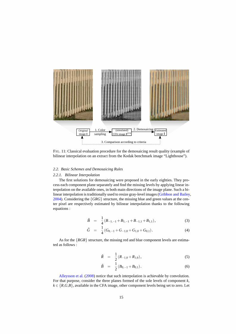
to the original imageI. Even this image is unavailable effectively,I is generally usedas a reference to evaluate the demosaicing quality. Then, one either strive to obtain as alow value as possible for an error criterion, or as a high value as possible for a qualitycriterion comparing the estimated image and the original one. A classical evaluationprocedure for the demosaicing result quality consists in (see figure11) :

1. simulating a CFA image provided by a mono-CCD camera from acolor originalimage provided by a three-CCD camera. This is achieved by sampling a singlecolor componentR, G or B at each pixel, according to the considered CFA arran-gement (Bayer CFA of figure9, in our case) ;

2. demosaicing this CFA image to obtain an estimated color image ;

3. comparing the original and estimated color images, so as to highlight artifactsaffecting the latter.

There is no general agreement on the demosaicing quality definition, which ishighly dependent upon the estimated color image exploitation – as will be detailed inthe next sections. In a first time, we will rely on visual examination, or else on the mostused quantitative criterion (signal-to-noise ratio) for aquality result evaluation, whichboth require a reference image. As in most works related to demosaicing, we will hereuse the Kodak image database (Kodak, 1991) as a benchmark forperformance com-parison of the various methods, as well as for illustration purposes. More precisely, toavoid overloaded results, a representative subset of twelve of these images has beenpicked up as the most used set in literature. These natural images contain rich colorsand textural regions, and are fully reproduced in figure37 so that they can be referredto in the text.

14

OriginalimageI

(simulated)CFA imageICFA

EstimatedimageI

1. Colorsampling

2. Demosaicing

3. Comparison according to criteria

FIG. 11: Classical evaluation procedure for the demosaicing result quality (example ofbilinear interpolation on an extract from the Kodak benchmark image “Lighthouse”).

2.2. Basic Schemes and Demosaicing Rules

2.2.1. Bilinear InterpolationThe first solutions for demosaicing were proposed in the early eighties. They pro-

cess each component plane separately and find the missing levels by applying linear in-terpolation on the available ones, in both main directions of the image plane. Such a bi-linear interpolation is traditionally used to resize gray-level images (Gribbon and Bailey,2004). Considering the{GRG} structure, the missing blue and green values at the cen-ter pixel are respectively estimated by bilinear interpolation thanks to the followingequations :

B =14

(B−1,−1 +B1,−1 +B−1,1 +B1,1) , (3)

G =14

(G0,−1 +G−1,0 +G1,0 +G0,1) . (4)

As for the{RGR} structure, the missing red and blue component levels are estima-ted as follows :

R =12

(R−1,0 +R1,0) , (5)

B =12

(B0,−1 +B0,1) . (6)

Alleysson et al.(2008) notice that such interpolation is achievable by convolution.For that purpose, consider the three planes formed of the sole levels of componentk,k∈ {R,G,B}, available in the CFA image, other component levels being set to zero. Let

15

R

G

G

R

R

GG

BB

BB

GG

GG

R

G

G

R

R

G

B

B

G

G

(a) ICFA

R

0

0

R

R

00

00

00

00

00

R

0

0

R

R

0

0

0

0

0

(b) ϕR(ICFA

)0

G

G

0

0

GG

00

00

GG

GG

0

G

G

0

0

G

0

0

G

G

(c) ϕG(ICFA

)0

0

0

0

0

00

BB

BB

00

00

0

0

0

0

0

0

B

B

0

0

(d) ϕB(ICFA

)

FIG. 12: Definition of planesϕk(ICFA

)by sampling the CFA image according to each

color componentk, k∈ {R,G,B}. The CFA image and planesϕk(ICFA

)are here colo-

rized for illustration sake.

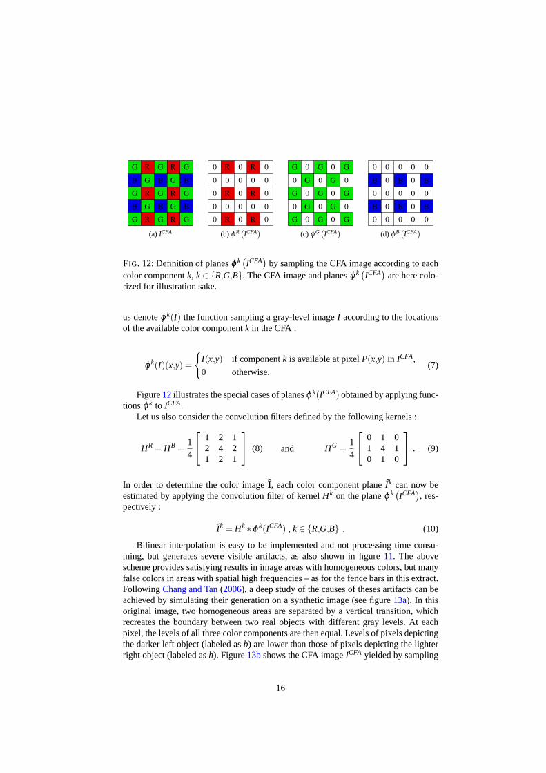
us denoteϕk(I) the function sampling a gray-level imageI according to the locationsof the available color componentk in the CFA :

ϕk(I)(x,y) =

{I(x,y) if componentk is available at pixelP(x,y) in ICFA,

0 otherwise.(7)

Figure12illustrates the special cases of planesϕk(ICFA) obtained by applying func-tionsϕk to ICFA.

Let us also consider the convolution filters defined by the following kernels :

HR = HB =14

1 2 12 4 21 2 1

(8) and HG =

14

0 1 01 4 10 1 0

. (9)

In order to determine the color imageI, each color component planeIk can now beestimated by applying the convolution filter of kernelHk on the planeϕk

(ICFA

), res-

pectively :

Ik = Hk ∗ϕk(ICFA) , k∈ {R,G,B} . (10)

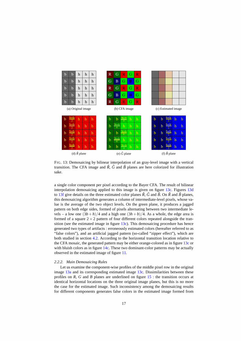
Bilinear interpolation is easy to be implemented and not processing time consu-ming, but generates severe visible artifacts, as also shownin figure 11. The abovescheme provides satisfying results in image areas with homogeneous colors, but manyfalse colors in areas with spatial high frequencies – as for the fence bars in this extract.Following Chang and Tan(2006), a deep study of the causes of theses artifacts can beachieved by simulating their generation on a synthetic image (see figure13a). In thisoriginal image, two homogeneous areas are separated by a vertical transition, whichrecreates the boundary between two real objects with different gray levels. At eachpixel, the levels of all three color components are then equal. Levels of pixels depictingthe darker left object (labeled asb) are lower than those of pixels depicting the lighterright object (labeled ash). Figure13bshows the CFA imageICFA yielded by sampling

16

hh

hh

hh

hh

hh

hb

hb

hb

hb

hb

b

b

b

b

b

(a) Original image

R

G

G

R

R

GG

BB

BB

GG

GG

R

G

G

R

R

R

G

G

R

R

(b) CFA image (c) Estimated image

h

h

h

h

h

h

h

h

h

h

b

b

b

b

b b+h2

b+h2

b+h2

b+h2

b+h2 h

h

h

h

h

(d) Rplane

h

h

h

h

h

hb

h

h

hb

hb

b

b

b

b

b

3h+b4

h

h

3h+b4

3h+b4

3b+h4

3b+h4

(e) G plane

h

h

h

h

h

hb

hb

hb

hb

hb

b

b

b

b

b b+h2

b+h2

b+h2

b+h2

b+h2

(f) B plane

FIG. 13: Demosaicing by bilinear interpolation of an gray-level image with a verticaltransition. The CFA image andR, G and B planes are here colorized for illustrationsake.

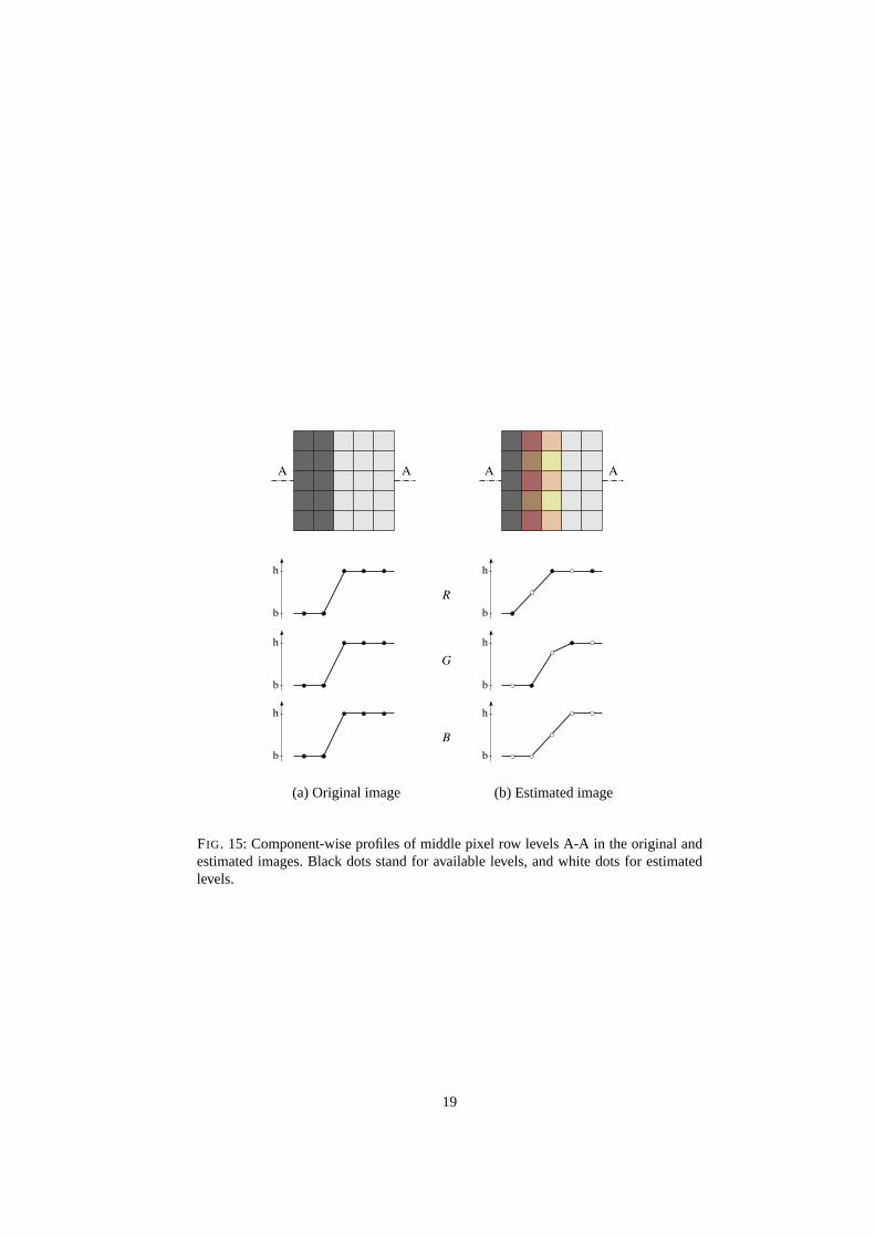
a single color component per pixel according to the Bayer CFA. The result of bilinearinterpolation demosaicing applied to this image is given onfigure 13c. Figures13dto 13f give details on the three estimated color planesR, G andB. On R andB planes,this demosaicing algorithm generates a column of intermediate-level pixels, whose va-lue is the average of the two object levels. On the green plane, it produces a jaggedpattern on both edge sides, formed of pixels alternating between two intermediate le-vels – a low one(3b+ h)/4 and a high one(3h+ b)/4. As a whole, the edge area isformed of a square 2×2 pattern of four different colors repeated alongside the tran-sition (see the estimated image in figure13c). This demosaicing procedure has hencegenerated two types of artifacts : erroneously estimated colors (hereafter referred to as“false colors”), and an artificial jagged pattern (so-called “zipper effect”), which areboth studied in section4.2. According to the horizontal transition location relativetothe CFA mosaic, the generated pattern may be either orange-colored as in figure13corwith bluish colors as in figure14c. These two dominant-color patterns may be actuallyobserved in the estimated image of figure11.

2.2.2. Main Demosaicing RulesLet us examine the component-wise profiles of the middle pixel row in the original

image13aand its corresponding estimated image13c. Dissimilarities between theseprofiles onR, G and B planes are underlined on figure15 : the transition occurs atidentical horizontal locations on the three original imageplanes, but this is no morethe case for the estimated image. Such inconsistency among the demosaicing resultsfor different components generates false colors in the estimated image formed from

17

hb

hb

hb

hb

hb

hb

hb

hb

hb

hb

b

b

b

b

b

(a) Refrence image

R

G

G

R

R

GG

BB

BB

GG

GG

R

G

G

R

R

R

G

G

R

R

(b) CFA image (c) Estimated image

FIG. 14: Variant version of image13a, demosaiced by bilinear interpolation as well.

their combination. It can also be noticed that the transition corresponds, in each colorplane of the original image, to a local change of homogeneityalong the horizontaldirection. Bilinear interpolation averages the levels of pixels located on both sides ofthe transition, which makes the latter less sharp.

In accordance with the previous observations, we can state that two main rules haveto be enforced so as to improve demosaicing results : spatialcorrelation and spectralcorrelation.

– Spectral correlation.The transition profiles plotted in figure15 are identical for the original imagecomponent planes, which conveys strict correlation between components. Fora natural image,Gunturk et al.(2002) show that the three color componentsare also strongly correlated. The authors apply a bidimensional filter built ona low-pass filterh0 = [1 2 1]/4 and a high-pass oneh1 = [1 −2 1]/4, so as tosplit each color component plane into four subbands resulting from row and co-lumn filtering : (LL) both rows and columns are low-pass filtered ; (LH) rowsare low-pass and columns high-pass filtered ; (HL) rows are high-pass and co-lumns low-pass filtered ; (HH) both rows and columns are high-pass filtered. Foreach color component, four subband planes are obtained in this way, respectivelyrepresenting data in rather homogeneous areas (low-frequency information), ho-rizontal detail (high-frequency information in the horizontal direction), verticaldetail (high-frequency information in the vertical direction) and diagonal detail(high-frequency information in both main directions). Theauthors then computea correlation coefficientrR,G between red and green components over each sub-band according to the following formula :

rR,G =

X−1∑

x=0

Y−1∑

y=0

(Rx,y−µR

)(Gx,y−µG

)

√X−1∑

x=0

Y−1∑

y=0(Rx,y−µR)2

√X−1∑

x=0

Y−1∑

y=0(Gx,y−µG)

2

, (11)

in whichRx,y (respectivelyGx,y) is the level at(x,y) pixel in the red (respectivelygreen) component plane within the same subband,µR andµG being the averageof Rx,y andGx,y levels over the same subband planes. The correlation coefficientbetween the blue and green components is similarly computed. Test results on

18

AA AA

R

G

B

h

b

h

b

h

b

h

b

h

b

h

b

(a) Original image (b) Estimated image

FIG. 15: Component-wise profiles of middle pixel row levels A-A in the original andestimated images. Black dots stand for available levels, and white dots for estimatedlevels.

19

twenty natural images show that those coefficients are always greater than 0.9in subbands carrying spatial high frequencies at least in one direction (i.e. LH,HL and HH). As for the subband carrying low frequencies (LL),coefficients arelower but always greater than 0.8. This reveals a very strong correlation bet-ween levels of different color components in a natural image, especially in areaswith high spatial frequencies.Lian et al.(2006) confirm, using a wavelet coef-ficient analysis, that high-frequency information is not only strongly correlatedbetween the three component planes, but almost identical. Suchspectral corre-lation between components should be taken into account to retrievethe missingcomponents at a given pixel.

– Spatial correlation.A color image can be viewed as a set of adjacent homogeneous regions whosepixels have similar levels for each color component. In order to estimate themissing levels at each considered pixel, one therefore should exploit the levelsof neighboring pixels. However, this task is difficult at pixels near the borderbetween two distinct regions due to high local variation of color components.As far as demosaicing is concerned, thisspatial correlationproperty avoids tointerpolate missing components at a given pixel thanks to neighbor levels whichdo not belong to the same homogeneous region.

These two principles are generally taken into account sequentially by the demo-saicing procedure. In the first step, demosaicing often consists in estimating the greencomponent using spatial correlation. According to Bayer’sassumption, the green com-ponent has denser available data within the CFA image, and represents the luminanceof the image to be estimated. Estimation of red and blue components (assimilated tochrominance) is only achieved in a second step, thanks to thepreviously interpola-ted luminance and using the spectral correlation property.Such a way of using bothcorrelations is used by a large number of methods in the literature. Also notice that, al-though red and blue component interpolation is achieved after the green plane has beenfully populated, spectral correlation is also often used inthe first demosaicing step toimprove the green plane estimation quality.

2.2.3. Spectral Correlation RulesIn order to take into account the strong spectral correlation between color com-

ponents at each pixel, two main hypotheses are proposed in the literature. The firstone assumes a colorratio constancy and the second one is based on colordifferenceconstancy. Let us examine the underlying principles of eachof these assumptions be-fore comparing both.

Interpolation based on color hue constancy, suggested byCok(1987), is historicallythe first one based on spectral correlation. According to Cok, hueis understood as theratio between chrominance and luminance, i.e.R/G or B/G. His method proceeds intwo steps. In the first step, missing green values are estimated by bilinear interpolation.Red (and blue) levels are then estimated by weighting the green level at the given pixelwith the hue average of neighboring pixels. For instance, interpolation of the blue levelat the center pixel of{GRG} CFA structure (see figure10a) uses the four diagonal

20

neighbors where this blue component is available :

B = G· 14

[B−1,−1

G−1,−1+

B1,−1

G1,−1+

B−1,1

G−1,1+

B1,1

G1,1

]. (12)

This bilinear interpolation between color component ratios is based on the localconstancy of this ratio within an homogeneous region.Kimmel (1999) justifies the co-lor ratio constancy assumption thanks to a simplified approach that models any colorimage as aLambertianobject surface observation. According to the Lambertian model,such a surface reflects the incident light to all directions with equal energy. The inten-sity I(P) received by the photosensor element associated to each pixel P is thereforeindependent of the camera position, and can be represented as :

I(P) = ρ⟨~N(P),~l

⟩, (13)

whereρ is the albedo (or reflection coefficient),~N(P) is the normal vector to the surfaceelement which is projected on pixelP, and~l is the incident light vector. As the albedoρcharacterizes the object material, this quantity is different for each color component(ρR 6= ρG 6= ρB), and the three color components may be written as :

IR(P) = ρR⟨~N(P),~l

⟩, (14)

IG(P) = ρG⟨~N(P),~l

⟩, (15)

IB(P) = ρB⟨~N(P),~l

⟩. (16)

Assuming that any object is composed of one single material,coefficientsρR, ρG

andρB are then constant at all pixels representing an object. So, the ratio between twocolor components is also constant :

Kk,k′ =Ik(P)

Ik′(P)=

ρk⟨~N(P),~l

⟩

ρk′⟨~N(P),~l

⟩ =ρk

ρk′ = constant, (17)

where(k,k′) ∈ {R,G,B}2. Although this assumption is simplistic, it is locally valid andcan be used within the neighborhood of the considered pixel.

Another simplified and widely used model of correlation between components re-lies on the colordifferenceconstancy assumption. At a given pixel, this can be writtenas :

Dk,k′ = Ik(P)− Ik′(P) = ρk⟨~N(P),~l

⟩−ρk′

⟨~N(P),~l

⟩= constant, (18)

where(k,k′) ∈ {R,G,B}2. As the incident light direction and amplitude are assumed tobe locally constant, the color component difference is alsoconstant within the consi-dered pixel neighborhood.

21

As a consequence, the chrominance interpolation step in Cok’s method may berewritten by using componentdifferenceaverages, for instance :

B = G+14

[(B−1,−1− G−1,−1)+(B1,−1− G1,−1)+(B−1,1− G−1,1)+(B1,1− G1,1)

],

(19)instead of equation (12). The validity of this approach is also justified byLian et al.(2007) on the ground of spatial high frequency similarity betweencolor components.

The color difference constancy assumption is globally consistent with the ratio ruleused in formula (12). By considering the logarithmic non-linear transformation, the

differenceDk,k′2 ,(k,k′) ∈ {R,G,B}2, can be expressed as :

Dk,k′2 = log10

(Ik(P)

Ik′(P)

)= log10

(Ik(P)

)− log10

(Ik′(P)

). (20)

Furthermore, we propose to compare those two assumptions expressed by equa-tions (17) and (18). In order to take into account spectral correlation for demosaicing,it turns out that the difference of color components presents some benefits in compa-rison to their ratio. The latter is indeed error-prone when its denominator takes lowvalues. This happens for instance when saturated red and/orblue components lead tocomparatively low values of green, making the ratios in equation (12) very sensitive tored and/or blue blue small variations. Figure16ais a natural image example which ishighly saturated in red. Figures16cand16dshow the images where each pixel valueis, respectively, the component ratioR/G and differenceR−G (pixel levels being nor-malized by linear dynamic range stretching). It can be noticed that these two imagesactually carry out less high-frequency information than the green component planeshown on figure16b.

A Sobel filter is then applied to these two images, so as to highlight the high-frequency information location. The Sobel filter output module is shown on figures16eand16f. In the right-hand parrot plumage area where red is saturated, the componentratio plane contains more high-frequency information thanthe component differenceplane, which makes it more artifact-prone when demosaiced by interpolation. Moreo-ver, high color ratio values may yield to estimated component levels beyond the databounds, which is undesirable for the demosaicing result quality.

To overcome these drawbacks, a linear translation model applied on all three colorcomponents is suggested byLukac and Plataniotis(2004a, 2004b). Instead of equa-tion (17), the authors reformulate the color ratio rule by adding a predefined constantvalueβ to each component. The new constancy assumption, which is consistent withequation (17) in homogeneous areas, now relies on the ratio :

Kk,k′2 =

Ik +βIk′ +β

, (21)

where(k,k′) ∈ {R,G,B}2, and whereβ ∈ N is a ratio normalization parameter. Underthis new assumption on the normalized ratio, the blue level interpolation formulated in

22

(a) Original image (b) G plane

(c) R/G ratio plane (d) R−G difference plane

(e) Sobel filter output on theR/G plane (f) Sobel filter output on theR−G plane

FIG. 16: Component ratio and difference planes on a same image (“Parrots” from theKodak database).

23

equation (12) under the ratio rule now becomes1 :

B = −β +(G+β

)· 14·[

B−1,−1 +βG−1,−1 +β

+B1,−1 +βG1,−1 +β

+B−1,1 +βG−1,1 +β

+B1,1 +βG1,1 +β

]. (22)

In order to avoid too different values for the numerator and denominator, Lukacand Plataniotis advise to setβ = 256, so that the normalized ratiosR/G andB/G rangefrom 0.5 to 2. They claim that this assumption improves the interpolation quality inareas of transitions between objects and of thin details.

In our investigation of the two main assumptions used for demosaicing, we finallycompare the estimated image quality in both cases. The procedure depicted on figure11is applied on twelve natural images selected from Kodak database : the demosaicingschemes presented above, respectively using component ratio and difference, are ap-plied to the simulated CFA image. To evaluate the estimated color image quality incomparison with the original image, we then compute an objective criterion, namelythe peak signal-to-noise ratio (PSNR) derived from the mean square error (MSE) bet-ween the two images. On the red plane for instance, these quantities are defined as :

MSER =1

XY

X−1

∑x=0

Y−1

∑y=0

(IRx,y− IR

x,y

)2, (23)

PSNRR = 10· log10

(2552

MSER

). (24)

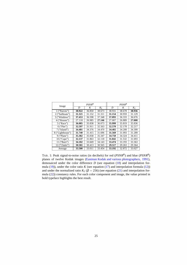
As the green component is bilinearly interpolated without using spectral correla-tion, only red and blue estimated levels vary according to the considered assumption.ThePSNRis hence computed on these two planes. Results displayed in table1 showthat using the color difference assumption yields better results than using the simpleratio ruleK, which is particularly noticeable for image “Parrots” of figure 16a. Thenormalized ratioK2, which is less prone to large variations thanK in areas with spatialhigh frequencies, leads to higher values forPSNRR andPSNRB. However, the colordifference assumption generally outperforms ratio-basedrules according to thePSNRcriterion, and is most often used to exploit spectral correlation in demosaicing schemes.

1The authors use, in this interpolation formula, extra weighting factors depending on the local pattern anddropped here for conciseness.

24

ImagePSNRR PSNRB

D K K2 D K K2

1 (“Parrots”) 38.922 36.850 38.673 38.931 38.678 38.9362 (“Sailboats”) 31.321 31.152 31.311 31.154 30.959 31.1293 (“Windows”) 37.453 36.598 37.348 37.093 36.333 36.6764 (“Houses”) 27.118 26.985 27.146 27.007 26.889 27.0085 (“Race”) 36.085 35.838 36.073 35.999 35.819 35.8366 (“Pier”) 32.597 31.911 32.563 32.570 32.178 32.217

7 (“Island”) 34.481 34.376 34.470 34.402 34.208 34.3998 (“Lighthouse”) 31.740 31.415 31.696 31.569 31.093 31.289

9 (“Plane”) 35.382 35.058 35.347 34.750 34.324 34.41110 (“Cape”) 32.137 31.863 32.118 31.842 31.532 31.69311 (“Barn”) 34.182 33.669 34.143 33.474 33.193 33.363

12 (“Chalet”) 30.581 30.413 30.565 29.517 29.263 29.364Average 33.500 33.011 33.454 33.192 32.872 33.027

TAB . 1: Peak signal-to-noise ratios (in decibels) for red (PSNRR) and blue (PSNRB)planes of twelve Kodak images (Eastman Kodak and various photographers, 1991),demosaiced under the color differenceD (see equation (18) and interpolation for-mula (19)), under the color ratioK (see equation (17) and interpolation formula (12))and under the normalized ratioK2 (β = 256) (see equation (21) and interpolation for-mula (22)) constancy rules. For each color component and image, the value printed inbold typeface highlights the best result.

25

3. Demosaicing Schemes

In this section, the main demosaicing schemes proposed in the literature are descri-bed. We distinguish two main procedures families, according to whether they scan theimage plane or chiefly use the frequency domain.

3.1. Edge-adaptive Demosaicing Methods

Estimating the green plane beforeR andB ones is mainly motivated by the doubleamount ofG samples in the CFA image. A fully populatedG component plane will sub-sequently make theR andB plane estimation more accurate. As a consequence, theGcomponent estimation quality becomes critical in the overall demosaicing performance,since any error in theG plane estimation is propagated in the following chrominanceestimation step. Important efforts are therefore devoted to improve the estimation qua-lity of the green component plane – usually assimilated to luminance –, especially inhigh-frequency areas. Practically, when the considered pixel lies on an edge betweentwo homogeneous areas, missing components should be estimated along the edge ratherthan across it. In other words, neighboring pixels to be taken into account for interpola-tion should not belong to distinct objects. When exploiting the spatial correlation, a keyissue is to determine the edge direction from CFA samples. Asdemosaicing methodspresented in the following text generally use specific directions and neighborhoods inthe image plane, some useful notations are introduced in figure17.

3.1.1. Gradient-based MethodsGradient computation is a general solution to edge direction selection. Hibbard’s

method (1995) uses horizontal and vertical gradients, computed at each pixel wherethe G component has to be estimated, in order to select the direction which providesthe best green level estimation. Let us consider the{GRG} CFA structure for instance(see figure10a). Estimating the green levelG at the center pixel is achieved in twosuccessive steps :

1. Approximate the gradient module (hereafter simply referred to asgradient forsimplicity) according to horizontal and vertical directions, as :

∆x = |G−1,0−G1,0| , (25)

∆y = |G0,−1−G0,1| . (26)

2. Interpolate the green level as :

G =

(G−1,0 +G1,0)/2 if ∆x < ∆y , (27a)

(G0,−1 +G0,1)/2 if ∆x > ∆y , (27b)

(G0,−1 +G−1,0 +G1,0 +G0,1)/4 if ∆x = ∆y. (27c)

Laroche and Prescott(1993) suggest to consider a 5×5 neighborhood for partialderivative approximations thanks to available surrounding levels, for instance∆x =|2R−R−2,0−R2,0|. Moreover,Hamilton and Adams(1997) combine both approaches.

26

−2

−1

1

2

−1−2 1 20 x

y

x′

y′

(a) Directions

−2

−1

1

2

−1−2 1 20 x

y(b) N4 neighborhood

−2

−1

1

2

−1−2 1 20 x

y(c) N′

4 neighborhood

P(δx,δy) ∈ N4 ⇔ (δx,δy) ∈ {(0,−1) , (−1,0) , (1,0) , (0,1)}P(δx,δy) ∈ N′

4 ⇔ (δx,δy) ∈ {(−1,−1) , (1,−1) , (−1,1) , (1,1)}

−2

−1

1

2

−1−2 1 20 x

y

(d) N8 neighborhood (N8 , N4∪N′4)

−2

−1

1

2

−1−2 1 20 x

y(e)N9 pixel set (N9 , N8∪P(0,0))

FIG. 17: Notations for the main spatial directions and considered pixel neighborhoods.

R−2,2 G−1,2 R0,2 G1,2 R2,2

G−2,1 B−1,1 G0,1 B1,1 G2,1

R−2,0 G−1,0 R0,0 G1,0 R2,0

G−2,−1 B−1,−1 G0,−1 B1,−1 G2,−1

R−2,−2 G−1,−2 R0,−2 G1,−2 R2,−2

FIG. 18: 5×5 neighborhood with central{GRG} structure in the CFA image.

27

To select the interpolation direction, these authors take into account both gradient andLaplacian second-order values by using the green levels available at nearby pixels andred (or blue) samples located 2 pixels apart. For instance, to estimate the green le-vel at {GRG} CFA structure (see figure18), Hamilton and Adams use the followingalgorithm :

1. Approximate the horizontal∆x and vertical∆y gradients thanks to absolute dif-ferences as :

∆x = |G−1,0−G1,0|+ |2R−R−2,0−R2,0| , (28)

∆y = |G0,−1−G0,1|+ |2R−R0,−2−R0,2| . (29)

2. Interpolate the green level as :

G =

(G−1,0 +G1,0)/2+(2R−R−2,0−R2,0)/4 if ∆x < ∆y, (30a)

(G0,−1 +G0,1)/2+(2R−R0,−2−R0,2)/4 if ∆x > ∆y, (30b)

(G0,−1 +G−1,0 +G1,0 +G0,1)/4

+(4R−R0,−2−R−2,0−R2,0−R0,2)/8 if ∆x = ∆y. (30c)

This proposal outperforms Hibbards’ method. Indeed, precision is gained not onlyby combining two color component data in partial derivativeapproximations, but alsoby exploiting spectral correlation in the green plane estimation. It may be noticed thatformula (30a) for the horizontal interpolation of green component may besplit into oneleft Gg and one rightGd side parts :

Gg = G−1,0 +(R−R−2,0)/2, (31)

Gd = G1,0 +(R−R2,0)/2, (32)

G =(

Gg + Gd)

/2. (33)

Such interpolation is derived from the color difference constancy assumption, andhence exploits spectral correlation for green component estimation. Also notice that,in these equations, horizontal gradients are assumed to be similar for both red and bluecomponents. A complete formulation has been given byLi and Randhawa(2005). Asthese authors show besides, the green component may more generally be estimatedby a Taylor series as long as green levels are considered as a continuous functiongwhich is differentiable in both main directions. The above equations (31) and (32)may then be seen as first-order approximations of this series. Indeed, inGg case forinstance, the horizontal approximation is written asg(x) = g(x− 1) + g′(x− 1) ≈g(x−1)+(g(x)−g(x−2))/2. Using the local constancy property of color componentdifference yieldsGx − Gx−2 = Rx −Rx−2, from which expression (31) is derived. Liand Randhawa suggest an approximation based on the second-order derivative,Gg es-timation becoming :

Gg = G−1,0 +(R−R−2,0)/2+(R−R−2,0)/4− (G−1,0−G−3,0)/4, (34)

28

for which a neighborhood size of 7×7 pixels is required. The additional term compa-red to (31) enables to refine the green component estimation. Similar reasoning maybe used to select the interpolation direction. According tothe authors, increasing theapproximation order in such a way improves estimation results under the mean squareerror (MSE) criterion.

Another proposal comes fromSu(2006), namely to interpolate the green level as aweighted sum of values defined by equations (30a) and (30b). Naming the latter respec-tively Gx = (G−1,0 +G1,0)/2+ (2R−R−2,0−R2,0)/4 andGy = (G0,−1 +G0,1)/2+(2R−R0,−2−R0,2)/4, horizontal and vertical interpolations are combined as :

G =

{w1 · Gx +w2 · Gy if ∆x < ∆y, (35a)

w1 · Gy +w2 · Gx if ∆x > ∆y, (35b)

wherew1 andw2 are the weighting factors. Expression (30c) remains unchanged (i.e.G =

(Gx + Gy

)/2 if ∆x = ∆y). The smallest level variation term must be weighted by

the highest factor (i.e.w1 > w2) ; expressions (30a) and (30b) incidentally correspond tothe special casew1 = 1, w2 = 0. Incorporating terms associated to high level variationsallows to undertake high-frequency information in the green component interpolationexpression itself. Su setsw1 to 0.87 andw2 to 0.13, since these weighting factor va-lues yield the minimal averageMSE (for the three color planes) over a large series ofdemosaiced images.

Other researchers, likeHirakawa and Parks(2005) or Menon et al.(2007), use thefilterbank approach in order to estimate missing green levels, before selecting the ho-rizontal or vertical interpolation direction at{GRG} and{GBG} CFA structures. Thisenables to design five-element mono-dimensional filters which are optimal towardscriteria specifically designed to avoid interpolation artifacts. The proposed optimal fil-ters (e.g.hopt = [−0.2569 0.4339 0.5138 0.4339 −0.2569] for Hirakawa and Parks’scheme) are close to the formulation of Hamilton and Adams2.

3.1.2. Component-consistent DemosaicingHamilton and Adam’s method selects the interpolation direction on the basis of ho-

rizontal and vertical gradient approximations. But this may be inappropriate, and unsa-tisfying results may be obtained in areas with textures or thin objects. Figure19showsan example where horizontal∆x and vertical∆y gradient approximations do not allowto take the right decision for the interpolation direction.Wu and Zhang(2004) proposea more reliable way to select this direction, still by using alocal neighborhood. Twocandidate levels are computed to interpolate the missing green value at a given pixel :one using horizontal neighbors, the second using vertical neighboring pixels. Then, themissingR or B value is estimated in both horizontal and vertical directions with eachof theseG candidates. A final step consists in selecting the most appropriate interpola-tion direction, namely that minimizing the gradient sum on the color difference planes(R−G andB−G) in the considered pixel neighborhood. This interpolationdirection

2No detail will be here given about howR andB components are estimated by the above methods, fortheir originality mainly lies in theG component estimation.

29

−1−2 1 20

50

100

200

250

150

−1−2 1 20

50

100

200

250

150

x

y

R

R R2,0R−2,0

R0,2R0,−2

G1,0G−1,0

G0,1G0,−1

∆x = |G−1,0−G1,0|+ |2R−R−2,0−R2,0| = 15

∆y = |G0,−1−G0,1|+ |2R−R−2,0−R2,0| = 17

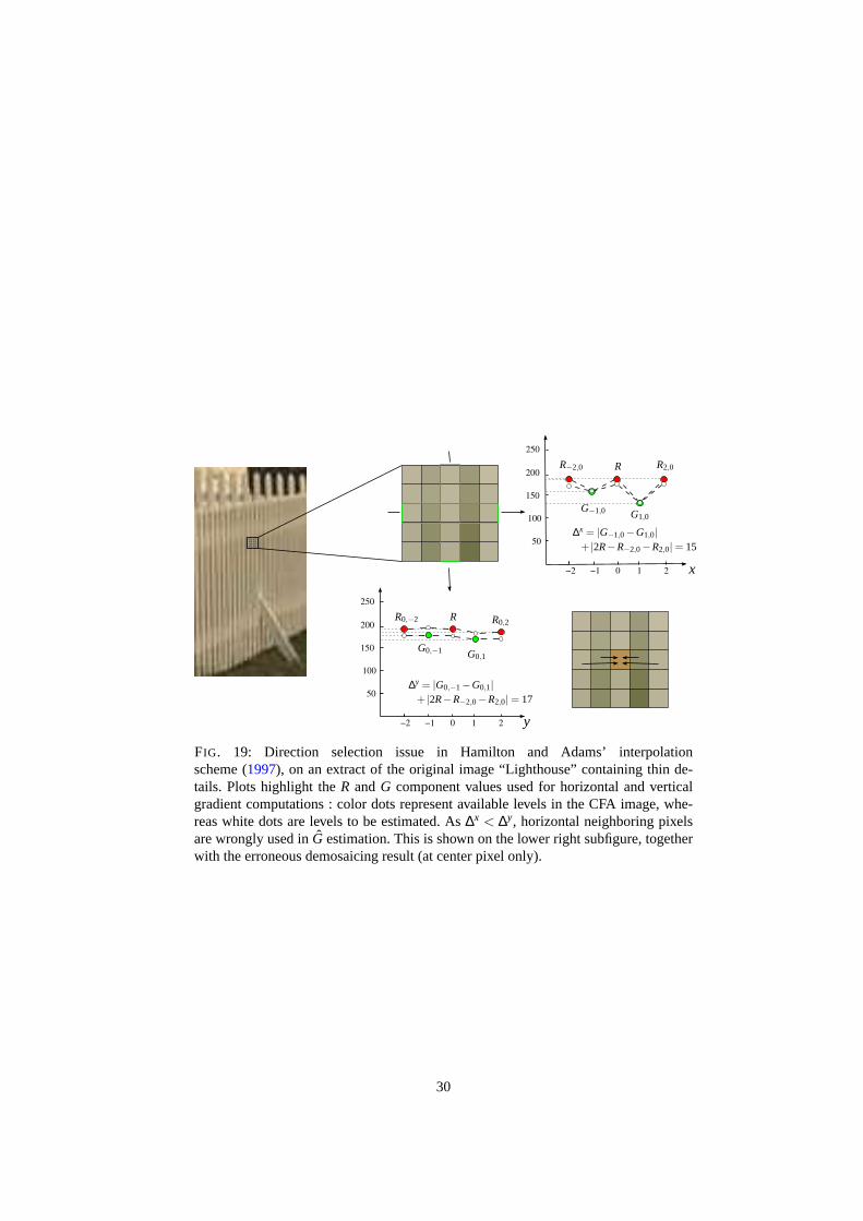
FIG. 19: Direction selection issue in Hamilton and Adams’ interpolationscheme (1997), on an extract of the original image “Lighthouse” containing thin de-tails. Plots highlight theR andG component values used for horizontal and verticalgradient computations : color dots represent available levels in the CFA image, whe-reas white dots are levels to be estimated. As∆x < ∆y, horizontal neighboring pixelsare wrongly used inG estimation. This is shown on the lower right subfigure, togetherwith the erroneous demosaicing result (at center pixel only).

30

allows to select the levels – computed beforehand – to be taken into account for themissing component estimation.

More precisely, Wu and Zhang’s approach proceeds in the following steps :

1. At each pixel where the green component is missing, compute two candidatelevels : one denoted asGx by using the horizontal direction (according to equa-tion (30a)), and anotherGy by using the vertical direction (according to (30b)).For other pixels, setGx = Gy = G.

2. At each pixel where the green component is available, compute two candidatelevels (one horizontal and one vertical) for each of the missing red and blue com-ponents. At{RGR} CFA structure these levels are expressed as (see figure10c) :

Rx = G+12(R−1,0− Gx

−1,0 +R1,0− Gx1,0), (36)

Ry = G+12(R−1,0− Gy

−1,0 +R1,0− Gy1,0), (37)

Bx = G+12(B0,−1− Gx

0,−1 +B0,1− Gx0,1), (38)

By = G+12(B0,−1− Gy

0,−1 +B0,1− Gy0,1). (39)

3. At each pixel with missing green component, compute two candidate levels forthe missing chrominance component (i.e.B at R samples, and conversely). At{GRG} CFA structure, the blue levels are estimated as (see figure10a) :

Bx = Gx +14 ∑

P∈N′4

(B(P)− Gx(P)), (40)

By = Gy +14 ∑

P∈N′4

(B(P)− Gy(P)), (41)

whereN′4 is composed of the four diagonal pixels (see figure17c).

4. Achieve the final estimation at each pixelP by selecting one component tripletout of the two candidates computed beforehand in both horizontal and verticaldirections. So as to use the direction for which variations of (R−G) and (B−G)component differences are minimal, the authors suggest thefollowing selectioncriterion :

(R,G,B) =

{(Rx,Gx,Bx) if ∆x < ∆y, (42a)

(Ry,Gy,By) if ∆x > ∆y, (42b)

where∆x and∆y are, respectively, the horizontal and vertical gradients on thedifference plane of estimated colors. More precisely, these gradients are com-puted by considering all distinct(Q,Q′) pixel pairs, respectively row-wise andcolumn-wise, within the 3×3 window centered at P (see figure17e) :

31

∆x = ∑(Q,Q′)∈N9×N9y(Q)=y(Q′)

∣∣(Rx(Q)− Gx(Q))−(Rx(Q′)− Gx(Q′)

)∣∣

+∣∣(Bx(Q)− Gx(Q)

)−(Bx(Q′)− Gx(Q′)

)∣∣ , (43)

∆y = ∑(Q,Q′)∈N9×N9x(Q)=x(Q′)

∣∣(Ry(Q)− Gy(Q))−(Ry(Q′)− Gy(Q′)

)∣∣

+∣∣(By(Q)− Gy(Q)

)−(By(Q′)− Gy(Q′)

)∣∣ . (44)

This method uses the same expressions as Hamilton and Adams’ones in order toestimate missing color components, but improves the interpolation direction decisionby using a 3×3 window – rather than a single row or column – in which the gradient ofcolor differences (R−G andB−G) is evaluated so as to minimize its local variation.

Among other attempts to refine the interpolation direction selection,Hirakawa and Parks(2005) propose a selection criterion which uses the number of pixels with homoge-neous colors in a local neighborhood. The authors compute the distances between thecolor point of the considered pixel and those of its neighbors in the CIEL∗a∗b∗ co-lor space (defined in section4.3.2), which better fits with the human perception ofcolors thanRGBspace. They design an homogeneity criterion with adaptive threshol-ding which reduces color artifacts due to incorrect selection of the interpolation di-rection.Chung and Chan(2006) nicely demonstrate that green plane interpolation iscritical to the estimated image quality, and suggest to evaluate the local variance ofcolor difference as an homogeneity criterion. The selecteddirection corresponds to mi-nimal variance, which yields green component refinement especially in textured areas.Omer and Werman(2004) use a similar way to select the interpolation direction, ex-cept that the local colorratio variance is used. These authors also propose a crite-rion based on a local corner score. Under the assumption thatdemosaicing generatesartificial corners in the estimated image, they apply the Harris corner detection fil-ter (Harris and Stephens, 1988), and select the interpolation direction which providesthe fewest detected corners.

3.1.3. Template Matching-based MethodsThis family of methods aims at identifying a template-basedfeature in each pixel

neighborhood, in order to interpolate according to the locally encountered feature. Suchstrategy has been first implemented by Cok in a patent dating back to 1986 (Cok,1986)(Cok, 1994), in which the author classifies 3×3 neighborhoods into edge, stripeor corner features (see figure20). The algorithm original part lies in the green com-ponent interpolation at each pixelP where it misses (i.e. at center pixel of{GRG} or{GBG} CFA structures) :

1. Compute the average green level available at the four nearest neighbor pixels ofP (i.e. belonging toN4, as defined on figure17b). Examine whether each of thesefour green levels is lower (b), higher (h), or equal to their average. Sort these four

32

values in descending order, letG1 > G2 > G3 > G4, and compute their medianM = (G2 +G3)/2.

2. ClassifyP neighborhood as :

(a) edgeif 3 h and 1b are present, or 1h and 3b (see figure20a) ;

(b) stripe if 2 h and 2b are present and opposite by pairs (see figure20b) ;

(c) corner if 2 h and 2b are present and adjacent by pairs (see figure20c).

In the special case when two values are equal to the average, the encounteredfeature is taken as :

(a) a stripe if the other two pixelsb andh are opposite ;

(b) an edge otherwise.

3. Interpolate the missing green level according to the previously identified feature :

(a) for an edge,G = M ;

(b) for a stripe,G= CLIPG2G3

(M− (S−M)), whereS is the average green levelover the eight neighboring pixels labeled asQ in figure20d;

(c) for a corner,G = CLIPG2G3

(M− (S′−M)), whereS′ is the average greenlevel over the four neighboring pixels labeled asQ in figure20e, which arelocated on both sides of the borderline betweenb andh pixels.

FunctionCLIPG2G3

simply limits the interpolated value to range[G3,G2] :

∀α ∈ R, CLIPG2G3

(α) =

α if G3 6 α 6 G2,

G2 if α > G2,

G3 if α < G3.

(45)

This method, which classifies neighborhood features into three groups, encom-passes three possible cases in an image. But the criterion used to distinguish the threefeatures is still too simple, and comparing green levels with their average may not besufficient to determine the existing feature adequately. Moreover, in case of astripefeature, interpolation does not take into account this stripe direction.

Chang and Tan(2006) also implement a demosaicing method based on template-matching, but apply it on the color difference planes (R−G andB−G) in order tointerpolateR andB color components,G being estimated beforehand thanks to Ha-milton and Adams’ scheme described above. The underlying strategy consists in si-multaneously exploiting the spatial and spectral correlations, and relies on a local edgeinformation which causes fewer color artifacts than Cok’s scheme. Although color dif-ference planes carry less high-frequency information thancolor component planes (seefigure 16), they can provide relevant edge information in areas with high spatial fre-quencies.

3.1.4. Adpative Weighted-Edge MethodMethods described above, as template-based or gradient-based ones, achieve inter-

polation according to the local context. They hence requireprior neighborhood clas-sification. The adaptive weighted-edge linear interpolation, first proposed byKimmel

33

h

h

bh P

(a) Edge

b

b

hh P

(b) Stripe

b

h

hb P

(c) Corner

b

b

hh P

Q

Q

Q

Q Q

Q

Q

Q

(d) Stripe neighborhood

b

h

hb P

Q

Q

Q

Q

(e) Corner neighborhood

FIG. 20: Feature templates proposed by Cok to interpolate the green component atpixel P. These templates, which are defined moduloπ/2, provide four possibleEdgeandCorner features, and two possibleStripefeatures.

(1999), is a method which merges these two steps into a single one. It consists in weigh-ting each locally available level by a normalized factor as afunction of a directionalgradient. For instance, interpolating the green level at center pixel of{GRG} or {GBG}CFA structures is achieved as :

G =w0,−1 ·G0,−1 +w−1,0 ·G−1,0 +w1,0 ·G1,0 +w0,1 ·G0,1

w0,−1 +w−1,0 +w1,0 +w0,1, (46)

wherewδx,δy coefficients are the weighting factors. In order to exploit spatial correla-tion, these weights are adjusted according to the locally encountered pattern.

Kimmel suggests to use local gradients to achieve weight computation. In a firststep, directional gradients are approximated at a CFA imagepixel P by using the levelsof its neighbors. Gradients are respectively defined in horizontal, vertical,x′-diagonal(top-right to bottom-left) andy′-diagonal (top-right to bottom-right) directions (seefigure17a) over a 3×3 neighborhood by the following generic expressions :

∆x(P) = (P1,0−P−1,0)/2, (47)

∆y(P) = (P0,−1−P0,1)/2, (48)

∆x′(P) =

max(∣∣∣(G1,−1−G)/

√2∣∣∣ ,∣∣∣(G−1,1−G)/

√2∣∣∣)

atG locations, (49a)

(P1,−1−P−1,1)/2√

2 elsewhere, (49b)

34

∆y′(P) =

max(∣∣∣(G−1,−1−G)/

√2∣∣∣ ,∣∣∣(G1,1−G)/

√2∣∣∣)

atG locations, (50a)

(P−1,−1−P1,1)/2√

2 elsewhere, (50b)

wherePδx,δy stands for the neighboring pixel ofP, with relative coordinates(δx,δy), inthe CFA image. Here,R, G or B is not specified, since these generic expressions applyto all CFA image pixels, whatever the considered available component. However, wenotice that all differences involved in equations (47) and (48) imply levels of a samecolor component.

The weightwδx,δy in directiond, d∈ {x,y,x′,y′}, is then computed from directionalgradients as :

wδx,δy =1√

1+∆d(P)2 +∆d(Pδx,δy)2, (51)

where directiond used to compute the gradient∆d is defined by the center pixelPand its neighborPδx,δy. At the right-hand pixel(δx,δy) = (1,0) as an example, thehorizontal directionx is used ford ; ∆d(P) and∆d(P1,0) are therefore both computedby expression (47) defining∆x, and the weight is expressed as :

w1,0 =1√

1+(P−1,0−P1,0)2/4+(P2,0−P)2/4. (52)

Definition of weightwδx,δy is built so that a local transition in a given directionyields a high gradient value in the same direction. Consequently, weightwδx,δy is closeto 0 for the neighborPδx,δy and does not contribute much to the final estimated greenlevel according to equation (46). On the opposite, weightwδx,δy is equal to 1 when thedirectional gradients are equal to 0.

Adjustments in weightw computation are proposed byLu and Tan(2003), whouse a Sobel filter to approximate the directional gradient, and the absolute – instead ofsquare – value of gradients in order to boost computation speed. Such a strategy is alsoimplemented byLukac and Plataniotis(2005b).

Once then green plane has been fully populated thanks to equation (46), red andblue levels are estimated by using component ratiosR/G andB/G among neighboringpixels. Interpolating the blue component is for instance achieved according to two steps(the red one being processed in a similar way) :

1. Interpolation at red locations (i.e. for{GRG} CFA structure) :

B= G·∑

P∈N′4

w(P) · B(P)

G(P)

∑P∈N′

4

w(P)= G·

w−1,−1 · B−1,−1

G−1,−1+w1,−1 · B1,−1

G1,−1+w−1,1 · B−1,1

G−1,1+w1,1 · B1,1

G1,1

w−1,−1 +w1,−1 +w−1,1 +w1,1.

(53)

35

2. Interpolation at other CFA locations with missing blue level (i.e. at{RGR} and{BGB} structures) :

B= G·∑

P∈N4

w(P) · B(P)

G(P)

∑P∈N4

w(P)= G·

w0,−1 · B0,−1

G0,−1+w−1,0 · B−1,0

G−1,0+w1,0 · B1,0

G1,0+w0,1 · B0,1

G0,1

w0,−1 +w−1,0 +w1,0 +w0,1.

(54)

Once all missing levels have been estimated, Kimmel’s algorithm (1999) achievesgreen plane refinement by using the color ratio constancy rule. This iterative refine-ment procedure is taken up byMuresan et al.(2000) with a slight modification : ins-tead of using allN8 neighboring pixels in step 1 below, only neighboring pixelswithgreen available component are considered. The following steps describe this refinementscheme :

1. Correct the estimated green levels with the average of twoestimations (one onthe blue plane, the other on the red one), so that the constancy rule is locallyenforced for color ratioG/R :

G =12

(GR+ GB) , (55)

where :

GR ,⌢

R·∑

P∈N4

w(P)·G(P)

R(P)

∑P∈N4

w(P) and GB ,⌢

B·∑

P∈N4

w(P)·G(P)

B(P)

∑P∈N4

w(P) ,

⌢

B and⌢

R standing either for an estimated level or an available CFA value, accor-ding to the considered CFA structure ({GRG} or {GBG}).

2. Correct then red and blue estimated levels at green locations, by using weightedR/G andB/G ratios at the eight neighboring pixels :

R= G·∑

P∈N8

w(P) ·⌢R(P)⌢G(P)

∑P∈N8

w(P)(56) and B = G·

∑P∈N8

w(P) ·⌢B(P)⌢G(P)

∑P∈N8

w(P). (57)

3. Repeat the two previous steps twice.

This iterative correction procedure gradually enforces more and more homoge-neousG/R andG/B color ratios, whereas the green component is estimated by usingspectral correlation. Its convergence is however not always guaranteed, which maycause trouble for irrelevant estimated values. When a level occurring in any color ratiodenominator is very close or equal to zero, the associated weight may not cancel theresulting bias. Figure21cshows some color artifacts which are generated in this case.In pure yellow areas, quasi-zero blue levels cause a saturation of the estimated greencomponent atRandB locations, which then alternate with original green levels.

Smith(2005) suggests to compute adaptive weights aswδx,δy = 11+4|∆d(P)|+4|∆d(Pδx,δy)|

,

in order to reduce the division bias and contribution of pixels on both edge sides.

36

(a) Original image (b) Estimated image before cor-rection

(c) Estimated image after cor-rection

FIG. 21: Demosaicing result achieved by Kimmel’s method (1999), before and afterthe iterative correction steps. Generated artifacts are pointed out on image(c).

Lukac et al.(2006) choose to apply adaptive weighting on colordifferenceplanes forRandB component estimations, which avoids the above-mentioned artifacts during theiterative correction step.Tsai and Song(2007) take up the latter idea, but enhance thegreen plane interpolation procedure : weights are adapted to the local topology thanksto a preliminary distinction between homogeneous and edge areas.

3.1.5. Local Covariance-based MethodsIn his PhD dissertation,Li (2000) presents an interpolation scheme to increase the

resolution of a gray-level image. Classical interpolationmethods (bilinear and bicu-bic), based on spatial invariant models, tend to blur transitions and generate artifacts inhigh-frequency areas. Li’s approach exploits spatial correlation by computing a locallevel covariance, without relying on directional gradients as do the above-mentionedmethods in this section. Beyond resolution enhancement, the author applies this ap-proach to demosaicing (Li and Orchard, 2001). In the CFA image, each ofR, G orB color component plane may be viewed as a sub-sampled versionof its respective,fully-populated estimated color plane. According to this consideration, a missing levelin a given color plane is interpolated by using local covariance, preliminarily estimatedfrom neighboring levels available in the same plane.

The underlying principle of this method may be better understood by consideringthe resolution enhancement problem first. More precisely, figure22 illustrates how theresolution of a gray-level image can be doubled thanks to geometric duality, in a two-step procedure. The first step consists in interpolatingP2i+1,2 j+1 level (represented by awhite dot in figure22a) from availableP2(i+k),2( j+l) levels (black dots). The followinglinear combination ofN′

4 neighbors is used here :

P2i+1,2 j+1 =1

∑k=0

1

∑l=0

α2k+l P2(i+k),2( j+l), (58)

in which αm coefficients, 06 m6 3, of ~α are computed as follows (see justification

37

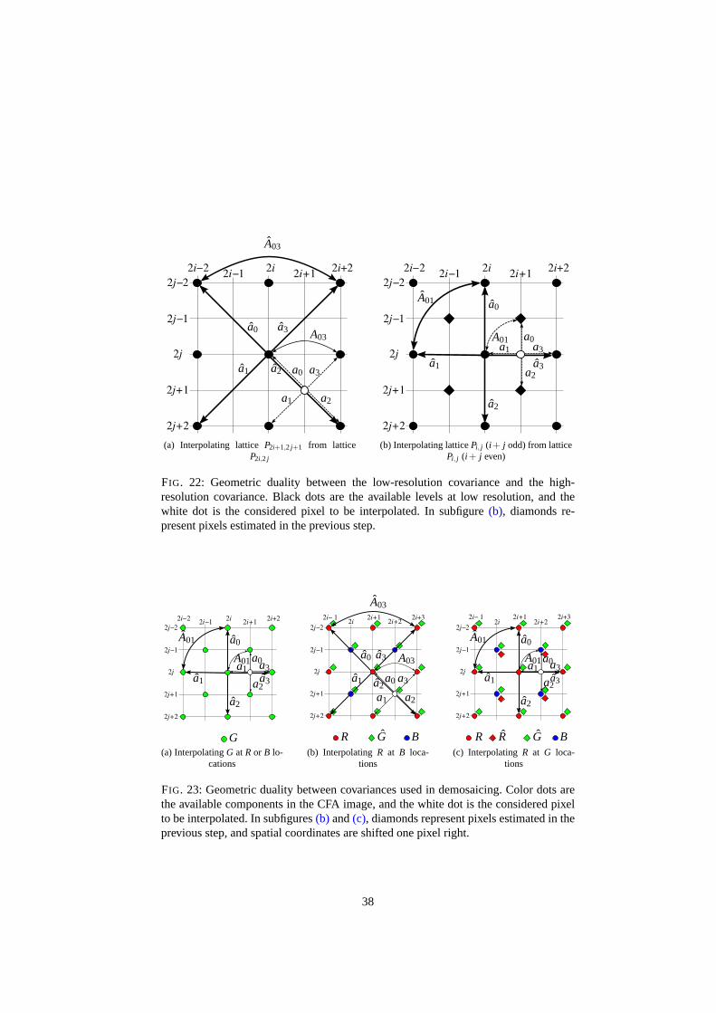
2i− 2 2i 2i+22i− 1 2i+1

2j− 2

2j

2j+2

2j− 1

2j+1

a0

a1 a2

a3

a0

a1 a2

a3

A03

A03

(a) Interpolating latticeP2i+1,2 j+1 from latticeP2i,2 j

2i− 2 2i 2i+22i− 1 2i+1

2j− 2

2j

2j+2

2j− 1

2j+1

a0

a1

a2

a3

a0a1

a2

a3

A01

A01

(b) Interpolating latticePi, j (i + j odd) from latticePi, j (i + j even)

FIG. 22: Geometric duality between the low-resolution covariance and the high-resolution covariance. Black dots are the available levelsat low resolution, and thewhite dot is the considered pixel to be interpolated. In subfigure (b), diamonds re-present pixels estimated in the previous step.

2i− 2 2i 2i+22i− 1 2i+1

2j− 2

2j

2j+2

2j− 1

2j+1

a0

a1

a2

a3

a0a1

a2

a3

A01

A01

G(a) InterpolatingG at R or B lo-

cations

2i− 1 2i+1 2i+32i 2i+2

2j− 2

2j

2j+2

2j− 1

2j+1

a0

a1 a2

a3

a0

a1 a2

a3

A03

A03

R BG(b) InterpolatingR at B loca-

tions

2i+1 2i+32i 2i+2

2j− 2

2j

2j+2

2j− 1

2j+1

2i− 1

a0

a1

a2

a3

a0a1

a2

a3

A01

A01

R BGR(c) InterpolatingR at G loca-

tions

FIG. 23: Geometric duality between covariances used in demosaicing. Color dots arethe available components in the CFA image, and the white dot is the considered pixelto be interpolated. In subfigures(b) and(c), diamonds represent pixels estimated in theprevious step, and spatial coordinates are shifted one pixel right.

38

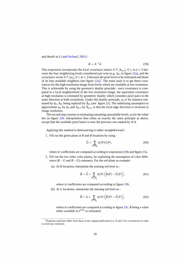
and details inLi and Orchard, 2001) :

~α = A−1~a. (59)

This expression incorporates the local covariance matrixA , [Am,n], 06 m,n 6 3 bet-ween the four neighboring levels considered pair-wise (e.g. A03 in figure22a), and thecovariance vector~a, [am], 06 m6 3 between the pixel level to be estimated and thoseof its four available neighbors (see figure22a)3. The main issue is to get these cova-riances for the high-resolution image from levels which areavailable at low resolution.This is achievable by using thegeometric dualityprinciple : once covariance is com-puted in a local neighborhood of the low-resolution image, the equivalent covarianceat high resolution is estimated by geometric duality which considers pixel pairs in thesame direction at both resolutions. Under this duality principle,a0 is for instance esti-mated by ˆa0, A03 being replaced byA03 (see figure22). The underlying assumption toapproximateam by am andAm,n by Am,n, is that the local edge direction is invariant toimage resolution.

The second step consists in estimating remaining unavailable levels, as for the whitedot on figure22b. Interpolation then relies on exactly the same principle asabove,except that the available pixel lattice is now the previous one rotated byπ/4.

Applying this method to demosaicing is rather straightforward :

1. Fill out the green plane atRandB locations by using :

G = ∑P∈N4

α(P)G(P), (60)

whereα coefficients are computed according to expression (59) and figure23a.

2. Fill out the two other color planes, by exploiting the assumption of color diffe-rence (R−G andB−G) constancy. For the red plane as example :

(a) At B locations, interpolate the missing red level as :

R= G+ ∑P∈N′

4

α(P)(

R(P)− G(P))

, (61)

whereα coefficients are computed according to figure23b.

(b) At G locations, interpolate the missing red level as :

R= G+ ∑P∈N4

α(P)(

⌢

R(P)− G(P))

, (62)

whereα coefficients are computed according to figure23c,⌢

Rbeing a valueeither available inICFA or estimated.

3Notations used here differ from those in the original publication (i.e.R and~r for covariances) in orderto avoid any confusion.

39

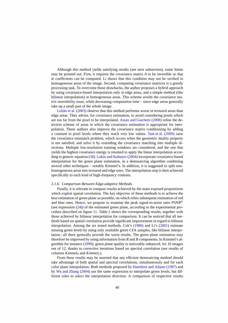
Although this method yields satisfying results (see next subsection), some limitsmay be pointed out. First, it requires the covariance matrixA to be invertible so thatα coefficients can be computed. Li shows that this condition may not be verified inhomogeneous areas of the image. Second, computing covariance matrices is a greedyprocessing task. To overcome those drawbacks, the author proposes a hybrid approachby using covariance-based interpolation only in edge areas, and a simple method (likebilinear interpolation) in homogeneous areas. This schemeavoids the covariance ma-trix invertibility issue, while decreasing computation time – since edge areas generallytake up a small part of the whole image.

Leitão et al.(2003) observe that this method performs worse in textured areas thanedge areas. They advise, for covariance estimation, to avoid considering pixels whichare too far from the pixel to be interpolated.Asuni and Giachetti(2008) refine the de-tection scheme of areas in which the covariance estimation is appropriate for inter-polation. These authors also improve the covariance matrixconditioning by addinga constant to pixel levels where they reach very low values.Tam et al.(2009) raisethe covariance mismatch problem, which occurs when the geometric duality propertyis not satisfied, and solve it by extending the covariance matching into multiple di-rections. Multiple low-resolution training windows are considered, and the one thatyields the highest covariance energy is retained to apply the linear interpolation accor-ding to generic equation (58). Lukin and Kubasov(2004) incorporate covariance-basedinterpolation for the green plane estimation, in a demosaicing algorithm combiningseveral other techniques – notably Kimmel’s. In addition, it is suggested to split non-homogeneous areas into textured and edge ones. The interpolation step is then achievedspecifically to each kind of high-frequency contents.

3.1.6. Comparison Between Edge-adaptive Methods.Finally, it is relevant to compare results achieved by the main exposed propositions

which exploit spatial correlation. The key objective of these methods is to achieve thebest estimation of green plane as possible, on which relies subsequent estimation of redand blue ones. Hence, we propose to examine the peak signal-to-noise ratioPSNRG

(see expression (24)) of the estimated green plane, according to the experimental pro-cedure described on figure11. Table2 shows the corresponding results, together withthose achieved by bilinear interpolation for comparison. It can be noticed that all me-thods based on spatial correlation provide significant improvement in regard to bilinearinterpolation. Among the six tested methods, Cok’s (1986) and Li’s (2001) estimatemissing green levels by using only available green CFA samples, like bilinear interpo-lation ; all three generally provide the worst results. The green plane estimation maytherefore be improved by using information fromRandB components. In Kimmel’s al-gorithm for instance (1999), green plane quality is noticeably enhanced, for 10 imagesout of 12, thanks to corrective iterations based on spectralcorrelation (see results ofcolumnsKimmel0 andKimmel1).

From these results may be asserted that any efficient demosaicing method shouldtake advantage of both spatial and spectral correlations, simultaneously and for eachcolor plane interpolation. Both methods proposed byHamilton and Adams(1997) andby Wu and Zhang(2004) use the same expression to interpolate green levels, but dif-ferent rules to select the interpolation direction. A comparison of respective results

40

Image Bilinear Hamilton Kimmel0 Kimmel1 Wu Cok Li1 38.982 44.451 40.932 28.244 44.985 39.320 39.9992 32.129 37.179 33.991 37.947 39.374 32.984 34.3053 37.477 43.161 39.870 38.207 43.419 38.161 38.7804 28.279 34.360 31.643 34.673 35.352 30.420 30.7055 36.709 42.603 39.291 41.477 43.515 38.103 38.8496 33.168 38.148 34.913 38.659 39.176 33.762 34.3547 35.682 40.650 37.605 40.978 43.121 36.734 38.3568 32.804 39.434 36.261 39.514 40.193 35.073 35.7479 35.477 40.544 37.470 39.603 41.013 36.219 36.65610 32.512 37.367 34.224 38.342 38.125 33.117 36.65611 34.308 38.979 35.934 38.321 39.194 34.837 35.10712 30.251 34.451 31.248 35.145 35.943 30.150 30.173

Average 33.981 39.277 36.115 37.592 40.284 34.907 35.807

TAB . 2: Peak Signal-to-Noise Ratio (in decibels) of the green plane (PSNRG), es-timated by various interpolation methods. For each image, the best result is prin-ted in bold typeface. Tested methods are here referred to chiefly by their first au-thor’s name : 1. Bilinear interpolation – 2. Hamilton and Adams’ gradient-basedmethod (1997) – 3 and 4. Kimmel’s adaptive weighted-edge method (1999), before(Kimmel0) and after (Kimmel1) corrective iterations – 5. Wu and Zhang’s component-consistent scheme (2004) – 6. Cok’s method based on template matching (1986) –7. Li’s covariance-based method (2001).

show that careful selection of the interpolation directionis important for overall perfor-mance. This is all the most noticeable that, compared to other algorithms, computationcomplexity is rather low for both Hamilton and Adams’ and Wu and Zhang’s methods.Indeed, they do not require any corrective iteration step nor covariance matrix estima-tion step, which are computation-expensive operations.

3.2. Estimated Color Correction

Once the two missing components have been estimated at each pixel, a post-processingstep of color correction is often applied to remove artifacts in the demosaiced image. Toremove false colors in particular, a classical approach consists in strengthening spectralcorrelation between the three estimated color components.Such a goal may be reachedfirst by median filtering, as described below. An iterative update of initial interpolatedcolors is also sometimes achieved, as Kimmel’s corrective step (1999) presented in sub-section3.1.4. A still more sophisticated algorithm proposed byGunturk et al.(2002)is described in detail in the second part of this section. Among other correction tech-niques of estimated colors,Li (2005) builds a demosaicing scheme by using a iterativeapproximation strategy with a spatially-adaptive stopping criterion ; he also studies theinfluence of the number of corrective iteration steps on the estimated image quality.Let us also mention here regularization schemes based on theBayesian framework, asMarkov Random Fields (see e.g.Mukherjee et al., 2001), which are however poorlyadapted to real-time implementation.

41

3.2.1. Median FilteringOne of the most widespread techniques in demosaiced image post-processing is

median filtering. Such a filter has been used for years to remove impulse noise in gray-level images, but also efficiently removes color artifacts without damaging local colorvariations.Freeman(1988) was the first person to take advantage of the median filterto remove demosaicing artifacts. Applied to the estimated planes of color differencesR−G andB−G, this filter noticeably improves the estimation provided bybilinearinterpolation. As shown on figure16d, these planes contain little high-frequency in-formation. False estimated colors, which result from inconsistency between the localinterpolation and those achieved in a neighborhood, may hence be more efficientlycorrected on these planes while preserving object edges.

Median filtering is implemented in several works of the demosaicing literature.For instance,Hirakawa and Parks(2005) propose to iterate the following correction– without giving more details about the number of iteration steps nor the filter kernelsize –, defined at each pixel as :

R′ = G+MRG, (63)

G′ =12

(R+MGR+ B+MGB) , (64)

B′ = G+MBG, (65)

whereR′, G′ andB′ denote the filtered estimated components, andMkk′ is the outputvalue of the median filter applied on estimated planes of color differencesIk − Ik′ ,(k,k′) ∈ {R,G,B}2. Lu and Tan(2003) use a slight variant of the latter, but advise toapply it selectively, since median filtering tends to attenuate color saturation in theestimated image. An appropriate strategy is proposed for the pre-detection of artifact-prone areas, where median filtering is then solely applied. However,Chang and Tan(2006) notice that median filtering applied to colordifferenceplanes, which still bearsome textures around edges, tends to induce “zipper” artifact in these areas. In order toavoid filtering across edges in the color difference planes,edge areas are preliminarilydetected thanks to a Laplacian filter.

Some artifacts may however remain in the median filtered image, which is mainlydue to separate filtering of color difference planes (R−G andB−G). An alternativemay be to apply a vector median filter on the estimated color image while exploitingspectral correlation. The local output of such a filter is thecolor vector which mini-mizes the sum of distances to all other color vectors in the considered neighborhood.But according toLu and Tan(2003), the vector filter brings out little superiority – ifany – in artifact removal, compared with the median filter applied to each color diffe-rence plane. The authors’ justification is that the estimation errors may be consideredas additive noise which corrupts each color plane. These noise vector components areloosely correlated. In such conditions,Astola et al.(1990) show that vector medianfiltering does not achieve better results than marginal filtering on the color differenceplanes.

42

3.2.2. Alternating Projection MethodAs previously mentioned in section2.2.3, pixel levels bear strong spectral corre-

lation in high spatial frequency areas of a natural color image. From this observation,Gunturk et al.(2002) aim at increasing the correlation of high-frequency informationbetween estimatedR, G andB component planes, while keeping the CFA image data.These two objectives are enforced by using two convex constraint sets, on which thealgorithm alternately projects estimated data. The first set is named “Observation” andensures that interpolated data are consistent with those available in the CFA image. Thesecond set, named “Detail”, is based on a decomposition of eachR, G andB plane intofour frequency subbands thanks to afilterbankapproach. A filterbank is a set of pass-band filters which decompose (analyze) the input signal into several subbands, eachone carrying the original signal information in a particular frequency subband. On theopposite, a signal may be reconstructed (synthesized) in a filterbank by recombinationof its subbands.

The algorithm uses an initially estimated image as startingpoint ; it may hence beconsidered as a – sophisticated – refinement scheme. To get the initial estimationI0,any demosaicing method is suitable. The authors suggest to use Hamilton and Adams’scheme to estimate the green planeIG

0 , and a bilinear interpolation to get the redIR0 and

blue IB0 planes. Two main steps are achieved then, as illustrated on figure24a:

1. Update the green plane by exploiting high-frequency information of red and blueplanes. This enhances the initial green component estimation.

(a) Use available red levels of the CFA image (orIR0 ) to form a downsampled

planeIR0 of sizeX/2×Y/2, as illustrated on figure24b.

(b) Sample, at the sameR locations, green levels from the initial estimationIG0

to form a downsampled planeIG(R)0 , also of sizeX/2×Y/2.

(c) Decompose the downsampled planeIR0 into four subbands :

IR,LL0 (x,y) = h0(x)∗

[h0(y)∗ IR

0 (x,y)], (66)

IR,LH0 (x,y) = h0(x)∗

[h1(y)∗ IR

0 (x,y)], (67)

IR,HL0 (x,y) = h1(x)∗

[h0(y)∗ IR

0 (x,y)], (68)

IR,HH0 (x,y) = h1(x)∗

[h1(y)∗ IR

0 (x,y)], (69)

and do the same with planeIG(R)0 . In their proposition, Gunturket al. use

a low-pass filterH0(z) and a high-pass filterH1(z) to analyze each planerespectively in low and high frequencies, as described above in subsec-tion 2.2.1.

(d) Use the low-frequency subband (LL) of IG(R)0 and the three subbands of

IR0 with high frequencies (LH, HL andHH) to synthesize a re-estimated

43

} }1 2 3 4 5 6 7

IG0

IB0

IB0

IR0

IR0 IR

1

IG1

IG1

IB1

IR

IG

IB

ICFA

IR0

IG(R)0

IG(B)0

IB0

IR,LL0

IR,LH0

IR,HL0

IR,HH0

IG(R),LL0

IG(R),LH0

IG(R),HL0

IG(R),HH0

IG(B),LL0

IG(B),LH0

IG(B),HL0

IG(B),HH0

IB,LL0

IB,LH0

IB,HL0

IB,HH0

IR,LL1

IR,LH1

IR,HL1

IR,HH1

IG,LL1

IG,LH1

IG,HL1

IG,HH1

IB,LL1

IB,LH1

IB,HL1

IB,HH1

IG(R)0

IG(B)0

IR1

IB1

≡

≡≡

Initialestim.

I0

Intermedia-te estim.

I1

Finalestim.

IG plane update

Iterations

Alternating projection ofRandB

(a) Procedure outline.G channel update :① Extraction of downsampledX/2×Y/2 planes (see details onfigure 24b) – ② Subband analysis of each downsampled plane –③ Synthesis of re-estimated downsampled

green planesIG(R)0 and IG(B)

0 at R andB locations –④ Insertion of these planes intoIG0 (see details on fi-

gure24c). Alternating projection ofR andB components :⑤ Subband analysis of intermediate estimationI1planes –⑥ Synthesis of re-estimated red and blue planes –⑦ Projection of these planes onto the “Observation”

constraint set (see details on figure24d).

RRRRRR

RRRRRR

RRRR

R

RR

RR

RR

RR

BBBBBB

BBBBBB

B

B

B

B

BB

BB

GG

GGG

G

G

G

GRGR

GRGR

GRGR

GRGR

GBGB

GBGB

IR0

IG0

IB0

IR0

IG(R)0

IB0

(b) Extraction of downsam-pled planes from initial esti-

mation.

GRGR

GRGR

GR

GR

GR

GR

GB

GB

GB

GB

GBGB

GBGB

GG

GGG

G

G

G

GG

GGG

G

G

G

GRGR

GRGR

GBGB

GBGB

IG(R)0

IG0 IG

1

IG(B)0

(c) Insertion of re-estimateddownsampled green planes

into IG0 .

R

R

R

R

RRRR

RR

R

RRRR

R

RRRR

RR

R

RRRR

R

B

B

B

B

BB

BBBB

BBBBBB

BB

BBBB

BBBBBB

RR

RR

R

R

R

R

GG

GGG

G

G

G

BB

BB

BB

BB

ICFA

IR1

IB1

IR

IB

(d) Projection of re-estimated redand blue planes onto the “Obser-

vation” set.

FIG. 24: Demosaicing procedure proposed byGunturk et al.(2002) from an initial es-timation I0.

44

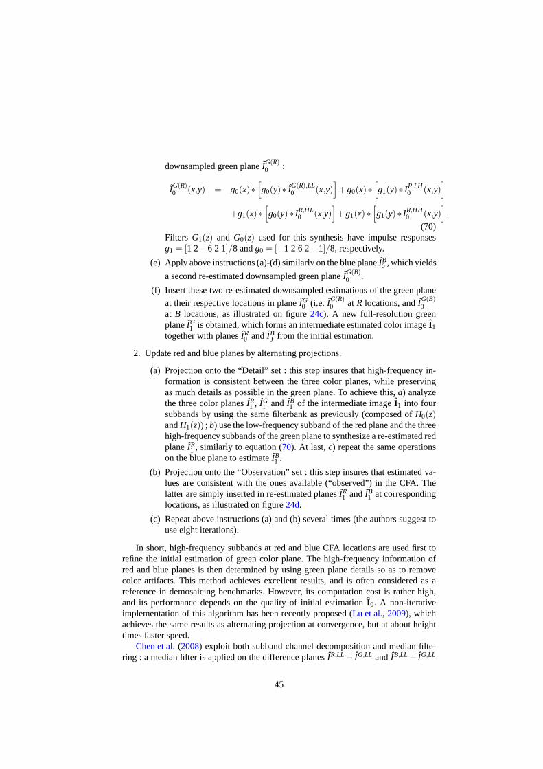
downsampled green planeIG(R)0 :

IG(R)0 (x,y) = g0(x)∗

[g0(y)∗ IG(R),LL

0 (x,y)]+g0(x)∗

[g1(y)∗ IR,LH

0 (x,y)]

+g1(x)∗[g0(y)∗ IR,HL

0 (x,y)]+g1(x)∗

[g1(y)∗ IR,HH

0 (x,y)].

(70)Filters G1(z) and G0(z) used for this synthesis have impulse responsesg1 = [1 2−6 2 1]/8 andg0 = [−1 2 6 2−1]/8, respectively.

(e) Apply above instructions (a)-(d) similarly on the blue planeIB0 , which yields

a second re-estimated downsampled green planeIG(B)0 .

(f) Insert these two re-estimated downsampled estimationsof the green plane

at their respective locations in planeIG0 (i.e. IG(R)

0 at R locations, andIG(B)0

at B locations, as illustrated on figure24c). A new full-resolution greenplaneIG

1 is obtained, which forms an intermediate estimated color imageI1

together with planesIR0 andIB

0 from the initial estimation.

2. Update red and blue planes by alternating projections.

(a) Projection onto the “Detail” set : this step insures thathigh-frequency in-formation is consistent between the three color planes, while preservingas much details as possible in the green plane. To achieve this, a) analyzethe three color planesIR

1 , IG1 and IB

1 of the intermediate imageI1 into foursubbands by using the same filterbank as previously (composed of H0(z)andH1(z)) ; b) use the low-frequency subband of the red plane and the threehigh-frequency subbands of the green plane to synthesize a re-estimated redplaneIR

1 , similarly to equation (70). At last,c) repeat the same operationson the blue plane to estimateIB

1 .

(b) Projection onto the “Observation” set : this step insures that estimated va-lues are consistent with the ones available (“observed”) inthe CFA. Thelatter are simply inserted in re-estimated planesIR

1 andIB1 at corresponding

locations, as illustrated on figure24d.

(c) Repeat above instructions (a) and (b) several times (theauthors suggest touse eight iterations).

In short, high-frequency subbands at red and blue CFA locations are used first torefine the initial estimation of green color plane. The high-frequency information ofred and blue planes is then determined by using green plane details so as to removecolor artifacts. This method achieves excellent results, and is often considered as areference in demosaicing benchmarks. However, its computation cost is rather high,and its performance depends on the quality of initial estimation I0. A non-iterativeimplementation of this algorithm has been recently proposed (Lu et al., 2009), whichachieves the same results as alternating projection at convergence, but at about heighttimes faster speed.

Chen et al.(2008) exploit both subband channel decomposition and median filte-ring : a median filter is applied on the difference planesIR,LL − IG,LL and IB,LL − IG,LL

45

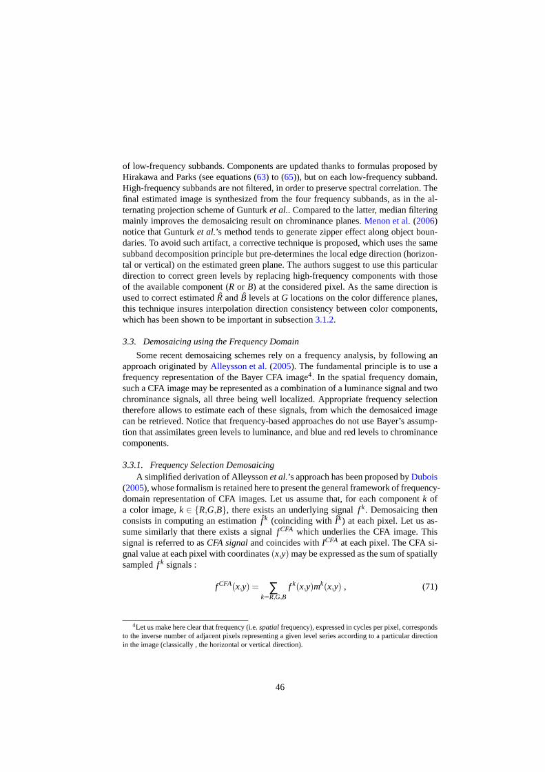
of low-frequency subbands. Components are updated thanks to formulas proposed byHirakawa and Parks (see equations (63) to (65)), but on each low-frequency subband.High-frequency subbands are not filtered, in order to preserve spectral correlation. Thefinal estimated image is synthesized from the four frequencysubbands, as in the al-ternating projection scheme of Gunturket al.. Compared to the latter, median filteringmainly improves the demosaicing result on chrominance planes.Menon et al.(2006)notice that Gunturket al.’s method tends to generate zipper effect along object boun-daries. To avoid such artifact, a corrective technique is proposed, which uses the samesubband decomposition principle but pre-determines the local edge direction (horizon-tal or vertical) on the estimated green plane. The authors suggest to use this particulardirection to correct green levels by replacing high-frequency components with thoseof the available component (R or B) at the considered pixel. As the same direction isused to correct estimatedR andB levels atG locations on the color difference planes,this technique insures interpolation direction consistency between color components,which has been shown to be important in subsection3.1.2.

3.3. Demosaicing using the Frequency Domain

Some recent demosaicing schemes rely on a frequency analysis, by following anapproach originated byAlleysson et al.(2005). The fundamental principle is to use afrequency representation of the Bayer CFA image4. In the spatial frequency domain,such a CFA image may be represented as a combination of a luminance signal and twochrominance signals, all three being well localized. Appropriate frequency selectiontherefore allows to estimate each of these signals, from which the demosaiced imagecan be retrieved. Notice that frequency-based approaches do not use Bayer’s assump-tion that assimilates green levels to luminance, and blue and red levels to chrominancecomponents.

3.3.1. Frequency Selection DemosaicingA simplified derivation of Alleyssonet al.’s approach has been proposed byDubois

(2005), whose formalism is retained here to present the general framework of frequency-domain representation of CFA images. Let us assume that, foreach componentk ofa color image,k ∈ {R,G,B}, there exists an underlying signalf k. Demosaicing thenconsists in computing an estimationf k (coinciding with Ik) at each pixel. Let us as-sume similarly that there exists a signalfCFA which underlies the CFA image. Thissignal is referred to asCFA signaland coincides withICFA at each pixel. The CFA si-gnal value at each pixel with coordinates(x,y) may be expressed as the sum of spatiallysampledf k signals :

fCFA(x,y) = ∑k=R,G,B

f k(x,y)mk(x,y) , (71)

4Let us make here clear that frequency (i.e.spatialfrequency), expressed in cycles per pixel, correspondsto the inverse number of adjacent pixels representing a givenlevel series according to a particular directionin the image (classically , the horizontal or vertical direction).

46

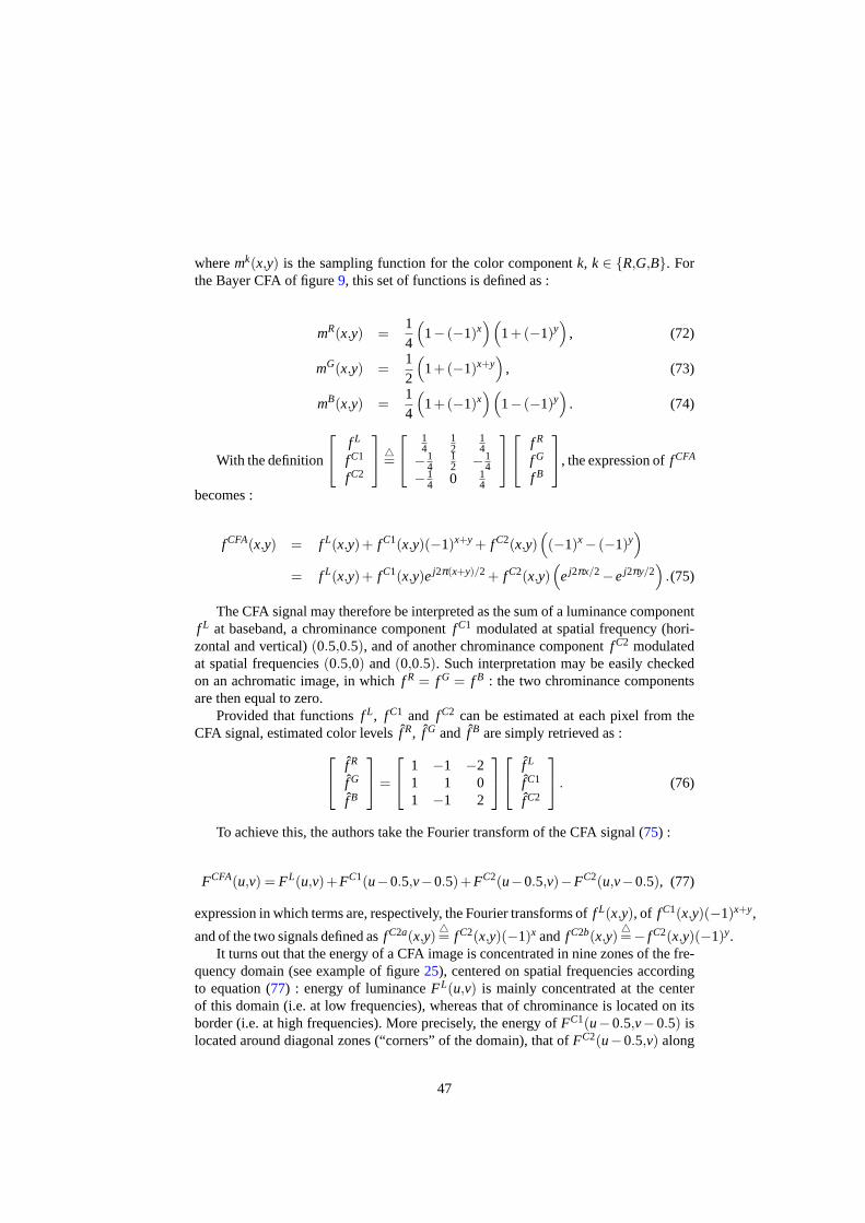
wheremk(x,y) is the sampling function for the color componentk, k ∈ {R,G,B}. Forthe Bayer CFA of figure9, this set of functions is defined as :

mR(x,y) =14

(1− (−1)x

)(1+(−1)y

), (72)

mG(x,y) =12

(1+(−1)x+y

), (73)

mB(x,y) =14

(1+(−1)x

)(1− (−1)y

). (74)

With the definition

f L

fC1

fC2

△

=

14

12

14

−14

12 −1

4−1

4 0 14

f R

f G

f B

, the expression offCFA

becomes :

fCFA(x,y) = f L(x,y)+ fC1(x,y)(−1)x+y + fC2(x,y)((−1)x− (−1)y

)

= f L(x,y)+ fC1(x,y)ej2π(x+y)/2 + fC2(x,y)(

ej2πx/2−ej2πy/2)

.(75)

The CFA signal may therefore be interpreted as the sum of a luminance componentf L at baseband, a chrominance componentfC1 modulated at spatial frequency (hori-zontal and vertical)(0.5,0.5), and of another chrominance componentfC2 modulatedat spatial frequencies(0.5,0) and(0,0.5). Such interpretation may be easily checkedon an achromatic image, in whichf R = f G = f B : the two chrominance componentsare then equal to zero.

Provided that functionsf L, fC1 and fC2 can be estimated at each pixel from theCFA signal, estimated color levelsf R, f G and f B are simply retrieved as :

f R

f G

f B

=

1 −1 −21 1 01 −1 2

f L

fC1

fC2

. (76)

To achieve this, the authors take the Fourier transform of the CFA signal (75) :

FCFA(u,v) = FL(u,v)+FC1(u−0.5,v−0.5)+FC2(u−0.5,v)−FC2(u,v−0.5), (77)

expression in which terms are, respectively, the Fourier transforms off L(x,y), of fC1(x,y)(−1)x+y,

and of the two signals defined asfC2a(x,y)△= fC2(x,y)(−1)x and fC2b(x,y)

△=− fC2(x,y)(−1)y.

It turns out that the energy of a CFA image is concentrated in nine zones of the fre-quency domain (see example of figure25), centered on spatial frequencies accordingto equation (77) : energy of luminanceFL(u,v) is mainly concentrated at the centerof this domain (i.e. at low frequencies), whereas that of chrominance is located on itsborder (i.e. at high frequencies). More precisely, the energy of FC1(u−0.5,v−0.5) islocated around diagonal zones (“corners” of the domain), that of FC2(u−0.5,v) along

47

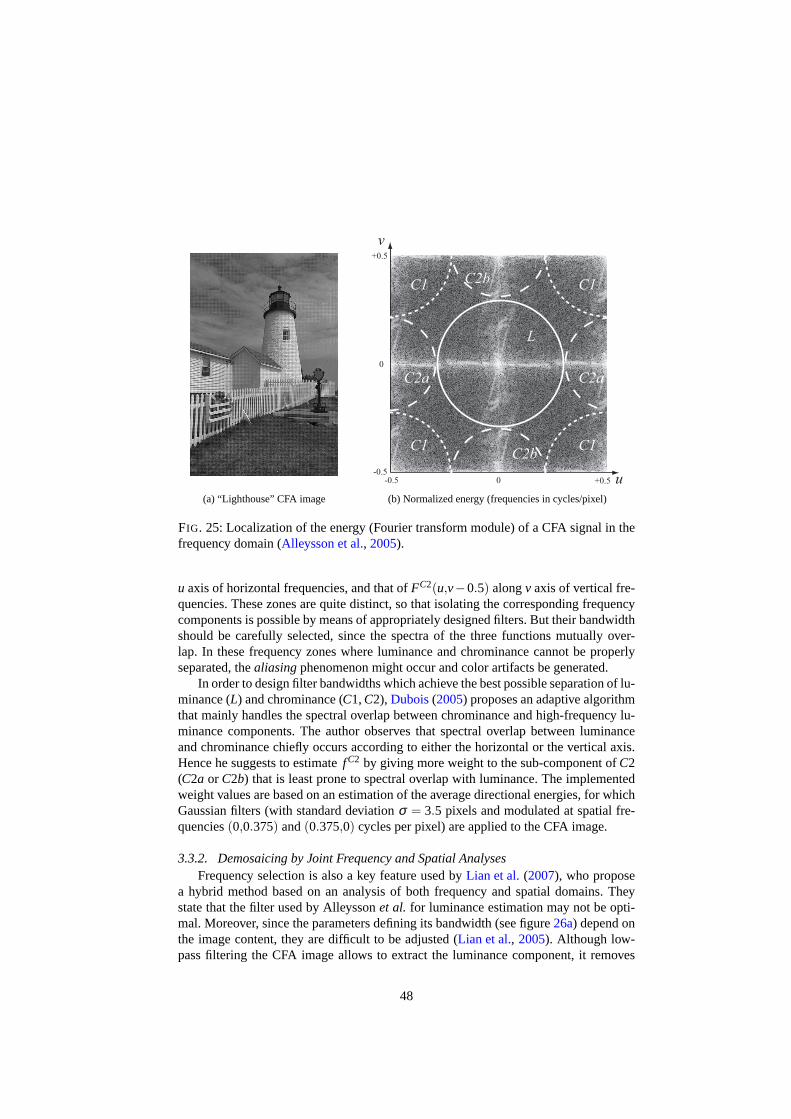
(a) “Lighthouse” CFA image

C1C1

C1

L

C2b

C2bC1

C2aC2a

v

u-0.5 0 +0.5

-0.5

0

+0.5

(b) Normalized energy (frequencies in cycles/pixel)

FIG. 25: Localization of the energy (Fourier transform module)of a CFA signal in thefrequency domain (Alleysson et al., 2005).

u axis of horizontal frequencies, and that ofFC2(u,v−0.5) alongv axis of vertical fre-quencies. These zones are quite distinct, so that isolatingthe corresponding frequencycomponents is possible by means of appropriately designed filters. But their bandwidthshould be carefully selected, since the spectra of the threefunctions mutually over-lap. In these frequency zones where luminance and chrominance cannot be properlyseparated, thealiasingphenomenon might occur and color artifacts be generated.

In order to design filter bandwidths which achieve the best possible separation of lu-minance (L) and chrominance (C1,C2), Dubois(2005) proposes an adaptive algorithmthat mainly handles the spectral overlap between chrominance and high-frequency lu-minance components. The author observes that spectral overlap between luminanceand chrominance chiefly occurs according to either the horizontal or the vertical axis.Hence he suggests to estimatefC2 by giving more weight to the sub-component ofC2(C2a or C2b) that is least prone to spectral overlap with luminance. Theimplementedweight values are based on an estimation of the average directional energies, for whichGaussian filters (with standard deviationσ = 3.5 pixels and modulated at spatial fre-quencies(0,0.375) and(0.375,0) cycles per pixel) are applied to the CFA image.

3.3.2. Demosaicing by Joint Frequency and Spatial AnalysesFrequency selection is also a key feature used byLian et al.(2007), who propose

a hybrid method based on an analysis of both frequency and spatial domains. Theystate that the filter used by Alleyssonet al. for luminance estimation may not be opti-mal. Moreover, since the parameters defining its bandwidth (see figure26a) depend onthe image content, they are difficult to be adjusted (Lian et al., 2005). Although low-pass filtering the CFA image allows to extract the luminance component, it removes

48

0

0.5

1

−0.5

0.5

0

u

Am

pli

tud

e

−0.5

0.5

0.5−0.5

−0.5

v

u

C2C1

LC2

r2

r1

0

v

0.5

(a) Alleyssonet al.

0

0

0.5

1

−0.5

0.5

0

uv

Am

pli

tude

1.5

−0.5

0.5

0.5−0.5

−0.5

v

u

C2C1

LC2

r1

0.5

(b) Lianet al. (filter used atG locations)

FIG. 26: Filters (bandwidth and spectrum) used to estimate luminance, as proposed byAlleysson et al.(2005) andLian et al.(2007).

the high-frequency information along horizontal and vertical directions. As the humaneye is highly sensitive to the latter, such loss is prejudicial to the estimation quality.Lian et al. then notice thatFC2 components in horizontal and vertical directions havesame amplitudes but opposite signs5. Consequently, the luminance spectrumFL at Glocations is obtained as the CFA image spectrum from whichC1 (“corner”) componenthas been removed (see details inLian et al., 2007). A low-pass filter is proposed to thispurpose, which cancelsC1 while preserving the high-frequency information along ho-rizontal and vertical axes. This filter is inspired from Alleyssonet al.’s, reproduced onfigure26a, but its bandpass is designed to removeC1 component only (see figure26b).The main advantage of this approach is that luminanceL spectrum bears less overlapwith the spectrum ofC1 than that ofC2 (see example of figure25b), which makes thefilter design easier.

From these observations, Lianet al.propose a demosaicing scheme with three mainsteps (see figure27) :

1. Estimate the luminance (denoted asL) at G locations, by applying a low-passfilter on the CFA image to removeC1. Practically, the authors suggest to use thefollowing 5×5 kernel, which gives very good results at low computationalcost :

H =164

0 1 −2 1 01 −4 6 −4 1

−2 6 56 6 −21 −4 6 −4 10 1 −2 1 0

. (78)

2. Estimate the luminance atR andB locations by a spatial analysis. As isolatingthe spectrum of componentC2 is rather difficult, the authors suggest an adaptivealgorithm based on color difference constancy (exploitingspectral correlation)and adaptive weighted-edge linear interpolation (exploiting spatial correlation) :

5We keep here notations used by Alleyssonet al. for C1 andC2, although switched by Lianet al.

49

... ... ... ...

...

...

...

... ... ... ...

...

...

...

... ... ... ...

...

...

...

... ... ... ...

...

...

...

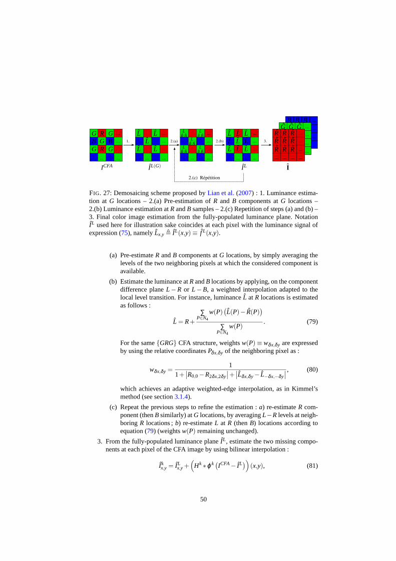
2.(a) 2.(b)

2.(c) Répétition

...

...

...

...

...

...

...

...

...

...

...

... ... ... ...

3.1.

R

RG

G

G

G

GBB L

R,BL

R,B

LR,B

LR,B

LR,B

LLL

LL

L

L

L

LL

L

L

L

L

RRRRRRRRR

GGGBBB

ICFA IL(G) IL I

FIG. 27: Demosaicing scheme proposed byLian et al.(2007) : 1. Luminance estima-tion at G locations – 2.(a) Pre-estimation ofR and B components atG locations –2.(b) Luminance estimation atRandB samples – 2.(c) Repetition of steps (a) and (b) –3. Final color image estimation from the fully-populated luminance plane. NotationIL used here for illustration sake coincides at each pixel withthe luminance signal ofexpression (75), namelyLx,y , IL(x,y) ≡ f L(x,y).

(a) Pre-estimateR andB components atG locations, by simply averaging thelevels of the two neighboring pixels at which the consideredcomponent isavailable.

(b) Estimate the luminance atRandB locations by applying, on the componentdifference planeL−R or L−B, a weighted interpolation adapted to thelocal level transition. For instance, luminanceL at R locations is estimatedas follows :

L = R+

∑P∈N4

w(P)(L(P)− R(P)

)

∑P∈N4

w(P). (79)

For the same{GRG} CFA structure, weightsw(P) ≡ wδx,δy are expressedby using the relative coordinatesPδx,δy of the neighboring pixel as :

wδx,δy =1

1+∣∣R0,0−R2δx,2δy

∣∣+∣∣Lδx,δy− L−δx,−δy

∣∣ , (80)

which achieves an adaptive weighted-edge interpolation, as in Kimmel’smethod (see section3.1.4).

(c) Repeat the previous steps to refine the estimation :a) re-estimateR com-ponent (thenB similarly) atG locations, by averagingL−R levels at neigh-boring R locations ;b) re-estimateL at R (thenB) locations according toequation (79) (weightsw(P) remaining unchanged).

3. From the fully-populated luminance planeIL, estimate the two missing compo-nents at each pixel of the CFA image by using bilinear interpolation :

Ikx,y = IL

x,y +(

Hk ∗ϕk(ICFA− IL))(x,y), (81)

50

whereϕk(I)(x,y), k∈ {R,G,B} is the plane defined by expression (7) and shownon figure12, and where convolution kernelsHk which achieve bilinear interpo-lation are defined by expressions (8) and (9)6.

The above approach does not require to design specific filtersin order to esti-mateC1 andC2 components, as do methods using the frequency domain only (Duboisuses for instance complementary asymmetric filters). Lianet al.show that their methodglobally outperforms other demosaicing schemes accordingto MSE (or PSNR) crite-rion. The key advantage seems to lie in exploiting the frequency domain atG locationsonly. According to results presented byLian et al.(2007), luminance estimations areless error-prone than green level estimations provided by methods which chiefly scanthe spatial image plane (shown in table2).

3.4. Conclusion

An introduction to the demosaicing issue and to its major solutions has been expo-sed in the above section. After having described why such a processing task is requiredin mono-CCD color cameras, the various CFA solutions have been presented. Focu-sing on the Bayer CFA, we have detailed the formalism in use throughout the paper.The simple bilinear interpolation has allowed us to introduce both artifact generationthat demosaicing method have to overcome, and two major rules widely used in theproposed approaches : spatial and spectral correlations.

The vast majority of demosaicing methods strive to estimatethe green plane first,which bear the most high-frequency information. The quality of this estimation stron-gly influences that of red and blue planes. When exploiting spatial correlation, we expe-rimentally show that a correct selection of the interpolation direction is crucial to reacha high interpolation quality for green levels. Moreover, component-consistent direc-tions should be enforced in order to avoid color artifact generation. Spectral correlationis often taken into account by interpolating on the difference, rather than ratio, of com-ponent planes. An iterative post-processing step of color correction is often achieved,so as to improve the final result quality by reinforcing spectral correlation.

Demosaicing methods may exploit spatial and/or frequency domains. The spatialdomain has been historically used first, and many studies arebased on it. More recently,authors exploit the frequency domain, which opens large perspectives. Such approachesindeed allow to avoid using – at least partially or in a first step – the heuristic rule ofcolor difference constancy to take spectral correlation into account. In all cases wheresuch assumptions are not fulfilled, even locally, exploiting the frequency domain is aninteresting solution. Dubois foresaw several years ago (2005) that frequency selectionapproaches are preeminently promising. This will be corroborated is the next sections,dedicated to the objective quality evaluation of images demosaiced by the numerouspresented methods. Already mentioned criteria (MSE andPSNR) will be completedby measures suited to human color perception, and new specific ones dedicated to thelocal detection of demosaicing artifacts.

6Notice thatϕk(I) may equally be expressed asϕk(I)(x,y) = I(x,y)mk(x,y), where sampling functionsmk

are defined by (72) to (74).

51

4. Objective Evaluation Criteria for Demosaiced Images

4.1. Introduction

The performances reached by different demosaicing schemesapplied to the sameCFA image can be very different. Indeed, different kinds of artifacts which alter theimage quality, can be generated by demosaicing schemes. A description of these arti-facts is given in subsection4.2.

Measuring the performance reached by a demosaicing scheme requires to evaluatethe quality of its output image. Indeed, such a measurement helps to compare the per-formances of the different schemes. For this purpose, we always follow the same ex-perimental procedure (see figure11). First, we simulate the color sampling by keepingonly one out of the three color components at each pixel of theoriginal imageI, accor-ding to the Bayer CFA mosaic. Then, we apply the considered demosaicing scheme toobtain the estimated color imageI (hereafter calleddemosaiced image) from the CFAsamples. Finally, we measure the demosaicing quality by comparing the original anddemosaiced images.

The main strategy of objective comparison is based on error estimation between theoriginal and demosaiced images. In subsection4.3, we present the most used criteriafor objective evaluation of the demosaiced image.

The objective criteria are generally based on a pixel-wise comparison between theoriginal and the estimated colors. These fidelity criteria are not specifically sensitiveto one given artifact. Hence, in subsection4.5, we present new measurements whichquantify the occurrences of demosaicing artifacts.

Since demosaicing methods intend to produce “perceptuallysatisfying” images,the most widely used evaluation criteria are based on the fidelity to the original images.Rather than displaying images, our goal is to apply automatic image analysis proce-dures to the demosaiced images in order to extract features.These extracted featuresare mostly derived from either colors or detected edges in the demosaiced images.Since the quality of features is sensitive to the presence ofartifacts, we propose toquantify the demosaicing performance by measuring the rates of erroneously detectededge pixels. This evaluation scheme is presented in the lastsubsection.

4.2. Demosaicing Artifacts

The main artifacts caused by demosaicing are blurring, false colors and zipper ef-fect. In this part, we present those artifacts on examples and explain their causes byconsidering the spatial and frequency domains.

4.2.1. Blurring ArtifactBlurring is located in areas where high frequency information, representing pre-

cise details or edges, is altered or erased. Figure28, illustrates different blurring levelsaccording to the used demosaicing scheme. A visual comparison between the originalimage28band image28cwhich has been demosaiced by bilinear interpolation, showsthat this scheme causes severe blurring. Indeed, some details of the parrot plumageare not retrieved by demosaicing and blurring is generated by low-pass filtering. Asstated in section2.2.1, this interpolation can be achieved by a convolution applied to

52

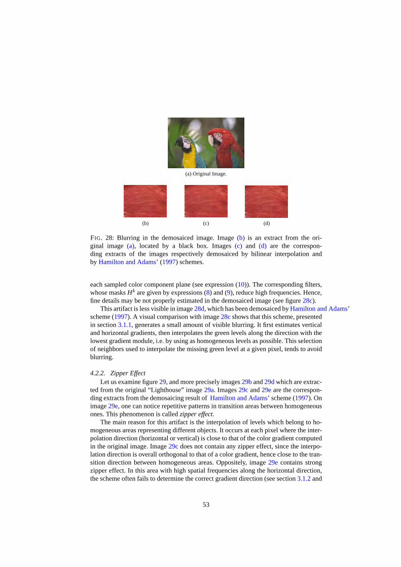
(a) Original Image.

(b) (c) (d)

FIG. 28: Blurring in the demosaiced image. Image(b) is an extract from the ori-ginal image(a), located by a black box. Images(c) and (d) are the correspon-ding extracts of the images respectively demosaiced by bilinear interpolation andby Hamilton and Adams’ (1997) schemes.

each sampled color component plane (see expression (10)). The corresponding filters,whose masksHk are given by expressions (8) and (9), reduce high frequencies. Hence,fine details may be not properly estimated in the demosaiced image (see figure28c).

This artifact is less visible in image28d, which has been demosaiced byHamilton and Adams’scheme (1997). A visual comparison with image28cshows that this scheme, presentedin section3.1.1, generates a small amount of visible blurring. It first estimates verticaland horizontal gradients, then interpolates the green levels along the direction with thelowest gradient module, i.e. by using as homogeneous levelsas possible. This selectionof neighbors used to interpolate the missing green level at agiven pixel, tends to avoidblurring.

4.2.2. Zipper EffectLet us examine figure29, and more precisely images29band29dwhich are extrac-

ted from the original “Lighthouse” image29a. Images29cand29eare the correspon-ding extracts from the demosaicing result ofHamilton and Adams’ scheme (1997). Onimage29e, one can notice repetitive patterns in transition areas between homogeneousones. This phenomenon is calledzipper effect.

The main reason for this artifact is the interpolation of levels which belong to ho-mogeneous areas representing different objects. It occursat each pixel where the inter-polation direction (horizontal or vertical) is close to that of the color gradient computedin the original image. Image29cdoes not contain any zipper effect, since the interpo-lation direction is overall orthogonal to that of a color gradient, hence close to the tran-sition direction between homogeneous areas. Oppositely, image29econtains strongzipper effect. In this area with high spatial frequencies along the horizontal direction,the scheme often fails to determine the correct gradient direction (see section3.1.2and

53

(b)

(d)

(a) Original image

(b) (c)

(d) (e)

(c)

(e)

(f) Demosaiced image

FIG. 29: Zipper effect due to erroneous selection of the interpolation direction.Images(b) and (d) are two extracts from the original image(a), located by blackboxes. Images(c) and(e)are the corresponding extracts from the image(f) demosaicedby Hamilton and Adams’s scheme (1997).

(b)

(a) Original image (b) (c)

(c)

(d) Demosaiced image

FIG. 30: False colors on a diagonal detail. Image(b) is an extract from the originalimage(a), located by a black box. Image(c), on which artifacts are circled in black,is the corresponding extract from image(d) demosaiced byHamilton and Adams’sscheme (1997).

figure19).The other main reason is related to the arrangement, in the CFA image, of pixels

whose green level is not available. Indeed, these pixels where the green levels can beerroneously estimated, are arranged in staggered locations.

4.2.3. False ColorsFalse color at a pixel corresponds to a large distance between the original color and

the estimated one, in the acquisition color spaceRGB. Figures30cand31cshow thatthis phenomenon is not characterized by a specific geometrical structure in the image.

Incorrect estimation of the color components may cause perceptible false colors, inparticular in areas with high spatial frequencies.

54

(a) Original Image (b) (c)

FIG. 31: False colors generated on a textured area.(b) Extract from the originalimage(a), located by a black box.(c) Extract demosaiced byWu and Zhangscheme(2004), with artifacts circled in black.

4.2.4. Artifacts Described in the Frequency DomainThe representation of the CFA color samples in the frequencydomain, proposed

by Alleysson et al.(2005), also allows to explain the reasons why artifacts are genera-ted by demosaicing schemes.

As seen in section3.3.1, the CFA image signal is made up of a luminance signal,mainly modulated at low spatial frequencies, and of two chrominance signals, mainlymodulated at high frequencies (see figure25 page48). Therefore, demosaicing canbe considered as an estimation of luminance and chrominancecomponents. Severalschemes which analyze the frequency domain (Alleysson et al., 2005; Dubois, 2005;Lian et al., 2007) estimate the missing levels by selective filters applied tothe CFAimage. The four possible artifacts caused by frequency analysis are shown in figure32extracted from (Alleysson et al., 2005) : excessive blurring, grid effect, false colorsand watercolor. When the bandwidth of the filter applied to theCFA image to estimatethe luminance is too narrow, an excessive blurring occurs inthe demosaiced image (seefigure32a). When the bandwidth of this filter is too wide, it may select high frequenciesin zones of chrominance. Such a case can result in a grid effect, especially visible in flat(homogeneous) areas of the image (see figure32b). Moreover, false colors appear whenthe chrominance filters overlap with the luminance filter in the frequency domain (seefigure32c). Finally, when the chrominance filter is too narrow, watercolor effect mayappear as colors which are “spread beyond” the edges of an object (see figure32d).

These artifacts are caused by a bad conception of the selective filters used to esti-mate luminance and chrominance. They can also be generated by demosaicing methodswhich spatially scan the image. Indeed, several spatial demosaicing schemes generateblurring and false colors since they tend to under-estimateluminance and over-estimatechrominance.Kimmel’s (1999) andGunturk et al.’s (2005) schemes also generate grideffect and watercolor.

4.3. Classical Objective Criteria

All the described artifacts are due to errors in color component estimation. Theclassical objective evaluation criteria sum up the errors between levels in the origi-nal and demosaiced images. At each pixel, the error between the original and demo-saiced images is quantized thanks to a distance between two color points in a three-dimensional color space (Busin et al., 2008). In this subsection, we regroup the most

55

(a) Blurring (b) Grid effect

(c) False color (d) Watercolor

FIG. 32: Four kinds of artifacts caused by demosaicing (Alleysson et al., 2005).

56

widely used measurements into two categories, namely the fidelity and perceptual cri-teria.

4.3.1. Fidelity CriteriaThese criteria use colors coded in theRGBacquisition color space in order to esti-

mate the fidelity of the demosaiced image compared with the original image.

1. Mean Absolute Error.This criterion evaluates the mean absolute error between the original imageI andthe demosaiced imageI. Denoted byMAE, it is expressed as (Chen et al., 2008;Li and Randhawa, 2005) :

MAE(I,I) =1

3XY ∑k=R,G,B

X−1

∑x=0

Y−1

∑y=0

∣∣∣Ikx,y− Ik

x,y

∣∣∣, (82)

whereIkx,y is the level of the color componentk at the pixel whose spatial coor-

dinates are(x,y) in the imageI. X andY are respectively the number of columnsand rows of the image.The MAE criterion can be used to measure the estimation errors of a specificcolor component. For example, this criterion is evaluated on the red color planeas :

MAER(I,I) =1

XY

X−1

∑x=0

Y−1

∑y=0

∣∣IRx,y− IR

x,y

∣∣. (83)

MAE values range from 0 to 255, and the demosaicing quality is considered asbetter as its value is low.

2. Mean Square Error.This criterion measures the mean quadratic error between the original imageand the demosaiced image. Denoted byMSE, it is defined as (Alleysson et al.,2005) :

MSE(I,I) =1

3XY ∑k=R,G,B

X−1

∑x=0

Y−1

∑y=0

(Ikx,y− Ik

x,y)2. (84)

The MSE criterion can also measure the error on each color plane, as in equa-tion (23). The optimal quality of demosaicing is reached whenMSEis equal to 0,whereas the worst is measured whenMSE is close to 2552.

3. Peak Signal-to-Noise Ratio.ThePSNRcriterion is a widely used distortion measurement to estimate the qua-lity of image compression. Many authors (e.g.Alleysson et al., 2005; Hirakawa and Parks,2005; Lian et al., 2007; Wu and Zhang, 2004) use this criterion to quantify theperformance reached by demosaicing schemes. ThePSNRis expressed in deci-bels as :

PSNR(I,I) = 10· log10

(d2

MSE(I,I)

), (85)

57

whered is the maximum color component level. When the color components arequantized with 8 bits,d is set to 255.Like the preceding criteria,PSNRcan be applied to a specific color plane. Forthe red color component, it is defined as :

PSNRR(I,I) = 10· log10

(d2

MSER(I,I)

). (86)

The higher thePSNRvalue is, the better is the demosaicing quality. ThePSNRmeasured on demosaiced images generally ranges from 30 to 40dB (i.e. MSEranges from 65.03 to 6.50).

4. Correlation.A correlation measurement between the original image and the demosaiced imageis used bySu and Willis(2003) to quantify the demosaicing performance. Thecorrelation criterion between two gray-level imagesI andI is expressed as :

C(I ,I) =

∣∣∣∣∣∣∣∣∣∣∣

(X−1∑

x=0

Y−1∑

y=0Ix,yIx,y

)−XYµµ

[(X−1∑

x=0

Y−1∑

y=0Ix,y2

)−XYµ2

]1/2[(X−1∑

x=0

Y−1∑

y=0Ix,y

2

)−XYµ2

]1/2

∣∣∣∣∣∣∣∣∣∣∣

, (87)

whereµ andµ are the mean gray levels in the two images.When a color demosaiced image is considered, one estimates the correlation le-vel Ck

(Ik, Ik

), k ∈ {R,G,B}, between the original and demosaiced color planes.

The mean of the three correlation levels is used to measure the quality of de-mosaicing. The correlation levelsC range between 0 and 1, and a measurementclose to 1 can be considered as a satisfying demosaicing quality.

4.3.2. Perceptual CriteriaThe preceding criteria are not well consistent with qualityestimation provided by

the human visual system. That is the reason why new measurements have been defined,which operate in perceptually uniform color spaces (Chung and Chan, 2006).

1. Estimation Error in the CIEL∗a∗b∗ color space.The CIEL∗a∗b∗ color space is recommended by the International Commissionon Illumination to measure the distance between two colors (Busin et al., 2008).This space is close to a perceptually uniform color space which has not beencompletely defined yet. So, the Euclidean distance in the CIEL∗a∗b∗ color spaceis a perceptual distance between two colors.The three color components(R,G,B) at a pixel are first transformed into(X,Y,Z)components according to a CIEXYZ linear operation. Then, the color compo-nents CIEL∗a∗b∗ are expressed as :

58

L∗ =

{116× 3

√Y/Yn−16 if Y/Yn > 0.008856, (88a)

903.3×Y/Yn otherwise, (88b)

a∗ = 500× ( f (X/Xn)− f (Y/Yn)) , (89)

b∗ = 200× ( f (Y/Yn)− f (Z/Zn)) , (90)

with :

f (x) =

{3√

x if Y/Yn > 0.008856 , (91a)

7.787x+ 16116 otherwise, (91b)

where the used reference white is characterized by the colorcomponents(Xn,Yn,Zn).We can notice thatL∗ represents the eye response to a specific luminance level,whereasa∗ andb∗ components correspond to chrominance. The componenta∗

represents an opposition of colors Red–Green, andb∗ corresponds to an opposi-tion of colors Blue–Yellow.The color difference is defined as the distance between two color points in thiscolor space. Then, the estimation error caused by demosaicing is the mean errorprocessed with all image pixels :

∆EL∗a∗b∗(I,I) =1

XY

X−1

∑x=0

Y−1

∑y=0

√∑

k=L∗,a∗,b∗

(Ikx,y− Ik

x,y

)2. (92)

The lower∆EL∗a∗b∗ is, the lower is the perceptual difference between the originaland demosaiced images, and the higher is the demosaicing quality.

2. Estimation Error in the S-CIEL∗a∗b∗ color space.In order to introduce spatial perception properties of the human visual system,Zhang and Wandell(1997) propose a new perceptual color space, called S-CIEL∗a∗b∗.The color components(R,G,B) are first transformed into the color spaceXYZwhich does not depend on the acquisition device. Then, thesecolor componentsare converted into the antagonist color spaceAC1C2, whereA represents the per-ceived luminance andC1,C2, the chrominance information in terms of oppositionof colors Red–Green and Blue–Yellow, respectively. The three component planesare then separately filtered by Gaussian filters with specificvariances, which ap-proximate the contrast sensitivity functions of the human visual system.The three filtered componentsA, C1 andC2 are converted back into(X,Y,Z)components, which are then transformed into CIEL∗a∗b∗ color space thanks toequations (88) and (89). Once the color componentsL∗, a∗ andb∗ have beencomputed, the estimation error∆E in S-CIEL∗a∗b∗ is defined by equation (92).This measurement was used byLi (2005), Su (2006) andHirakawa and Parks(2005) to measure the demosaicing quality.

59

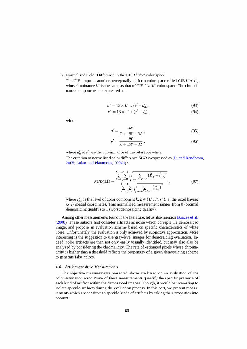
3. Normalized Color Difference in the CIEL∗u∗v∗ color space.The CIE proposes another perceptually uniform color space called CIEL∗u∗v∗,whose luminanceL∗ is the same as that of CIEL∗a∗b∗ color space. The chromi-nance components are expressed as :

u∗ = 13×L∗× (u′−u′n), (93)

v∗ = 13×L∗× (v′−v′n), (94)

with :

u′ =4X

X +15Y +3Z, (95)

v′ =9Y

X +15Y +3Z, (96)

whereu′n etv′n are the chrominance of the reference white.The criterion of normalized color differenceNCD is expressed as (Li and Randhawa,2005; Lukac and Plataniotis, 2004b) :

NCD(I,I) =

X−1∑

x=0

Y−1∑

y=0

√∑

k=L∗,u∗,v∗

(Ikx,y− Ik

x,y

)2

X−1∑

x=0

Y−1∑

y=0

√∑

k=L∗,u∗,v∗

(Ikx,y

)2, (97)

whereIkx,y is the level of color componentk, k∈ {L∗,u∗,v∗}, at the pixel having

(x,y) spatial coordinates. This normalized measurement ranges from 0 (optimaldemosaicing quality) to 1 (worst demosaicing quality).

Among other measurements found in the literature, let us also mentionBuades et al.(2008). These authors first consider artifacts as noise which corrupts the demosaicedimage, and propose an evaluation scheme based on specific characteristics of whitenoise. Unfortunately, the evaluation is only achieved by subjective appreciation. Moreinteresting is the suggestion to use gray-level images for demosaicing evaluation. In-deed, color artifacts are then not only easily visually identified, but may also also beanalyzed by considering the chromaticity. The rate of estimated pixels whose chroma-ticity is higher than a threshold reflects the propensity of agiven demosaicing schemeto generate false colors.

4.4. Artifact-sensitive Measurements

The objective measurements presented above are based on an evaluation of thecolor estimation error. None of these measurements quantify the specific presence ofeach kind of artifact within the demosaiced images. Though,it would be interesting toisolate specific artifacts during the evaluation process. In this part, we present measu-rements which are sensitive to specific kinds of artifacts bytaking their properties intoaccount.

60

0

50

100

150

200

250

100 110 120 130 140 150 160 170 180

Pl1

P1Pr

1 ≡ Pl2

P2Pr

2 Pl3

P3Pr

3 ≡ Pl4

P4Pr

4

x spatial coordinate

Lle

vel

FIG. 33: Vertical edge pixels associated with their left and right pixels. Vertical edgepixels P1, P2, P3 andP4 are represented by solid lines, while pixels correspondingtoextrema are located by dashed lines. The left (resp. right) extremum of a vertical edgepixel Pi is denotedPl

i (resp.Pri ). One single extremum may be associated with two

different vertical edge pixels, for examplePr1 ≡ Pl

2.

4.4.1. Blurring MeasurementThe blurring measurement proposed byMarziliano et al.(2004) is sensitive to the

decrease of local level variations in transition areas. Theauthors notice that blurringcorresponds to an expansion of these transition areas, and propose to measure the tran-sition widths to quantify this artifact. The evaluation scheme analyzes the luminanceplanes of the original and demosaiced images, respectivelydenoted asL and L. Thetransition width increase, evaluated at the same pixel locations in both images, yieldsan estimation of the blurring caused by demosaicing.

This blurring measurement consists in the following successive steps :

1. Apply the Sobel filter to the luminance planeL according to the horizontal direc-tion, and threshold its output. The pixels detected in this way are calledverticaledge pixels.

2. At each vertical edge pixelP, examine the luminance levels of pixels located onthe same row asP in the luminance planeL. The pixelPl (resp.Pr ) correspondsto the first local luminance extremum located on the left (resp. the right) ofP.To each vertical edge pixelP, associate in this way a pair of pixelsPl andPr ,one of them corresponding to a local luminance maximum and the other one toa minimum (see figure33).

3. The transition width atP is defined as the difference between thex coordinates

61

of pixelsPl andPr .

4. Compute the blurring measurement as the mean transition width estimated overall vertical edge pixels in the image.

5. From the spatial locations of vertical edge pixels inL – which have been detectedin step 1 –, steps 2 to 4 are performed on the luminance planeL of the demosaicedimage. A blurring measurement is then obtained for this plane.

6. The two measurements, obtained respectively for the original and demosaicedimages, are compared in order to estimate blurring caused bythe considereddemosaicing scheme.

4.4.2. Zipper Effect MeasurementsAs far as we know, the single proposition for zipper effect measurement was gi-

ven byLu and Tan(2003). This artifact is characterized at a pixel by an increase ofthe minimal distance between its color and those of its neighbors. This measurementtherefore relates to the original color image.

The zipper effect measurement in a demosaiced imageI, compared with the originalimageI, is computed by these successive steps :

1. At each pixelP in the original imageI, identify the neighboring pixelP′ whosecolor is the closest to that ofP in CIE L∗a∗b∗ color space :

P′ = argminQ∈N8

‖I(P)− I(Q)‖ , (98)

whereN8 is the 8-neighborhood ofPand‖·‖ is the Euclidean distance in CIEL∗a∗b∗

color space. The color difference is then computed as :

∆I(P) =∥∥I(P)− I(P′)

∥∥ . (99)

2. At the same locations asP andP′, compute their color difference in the demo-saiced imageI :

∆I(P) =∥∥I(P)− I(P′)

∥∥ . (100)

3. Compute the color difference variationϕ(P) = ∆I(P)−∆I(P).

4. Threshold the color difference variation, in order to detect the pixelsP wherezipper effect occurs. If|ϕ(P)|> Tϕ , the pixelP in the demosaiced image presentsa high variation of the difference between its color and thatof P′. More precisely,whenϕ(P) is lower than−Tϕ , the demosaicing scheme has reduced the colordifference between pixelsP andP′. On the other hand, whenϕ(P) > Tϕ , thedifference between the color ofP and that ofP′ has been highly increased inIcompared withI ; so, the pixelP is considered as affected by zipper effect. Theauthors propose to set the thresholdTϕ to 2.3

5. Compute the rate of pixels affected by zipper effect in thedemosaiced image :

ZE% = Card{

P(x,y) | ϕ(P) > Tϕ}

. (101)

62

(a) Original imageI (b) Demosaiced imageI (c) Zipper effect map

FIG. 34: Over-detection of the zipper effect byLu and Tan’s measurement (2003), in asynthetic image.In the detection map(c), pixels affected by zipper effect are labeled as×, and theground-truth (determined by visual examination) is labeled as gray. A pixel labeledboth as× and gray corresponds to a correct detection, whereas a pixellabeled only as× corresponds to an over-detection of the zipper effect.

The effectiveness of this measurement was illustrated by its authors with a syn-thetic image7. However, by applying it to images of Kodak Database, we willshowin section5.2 that it tends to over-detect zipper effect in the demosaicedimages. Tworeasons explain this over-detection.

First, a pixel whose color is correctly estimated and which has neighboring pixelswhose colors are erroneously estimated, can be considered as being affected by zippereffect (see figure34).

Second, we notice that all the pixels detected by Lu and Tan’smeasurement are notlocated in areas with perceptible alternating patterns which correspond to zipper effect.Indeed, all the artifacts which can increase the minimal difference between the color ofa pixel and those of its neighbors do not always bear the geometric properties of zippereffect. An example of this phenomenon is found on the zipper effect detection resultof figure38c4: almost all pixels are detected as affected by zipper effect, although thedemosaiced image38b4does not contain this repetitive and alternating pattern.

To avoid over-detection, we propose a scheme – hereafter referred to asdirectionalalternation measurement– which quantifies the level variations over three adjacentpixels along the horizontal or vertical direction in the demosaiced image.

Two reasons explain why the direction of zipper effect is mainly horizontal or ver-tical. Demosaicing schemes usually estimate the green color component first, then thered and blue ones by using color differences or ratios. However, along a diagonal direc-tion in the CFA image, all the green levels are either available or missing. Since thereis no alternating pattern between estimated and available levels along this diagonaldirection, there are few alternating estimation errors which characterize zipper effect.Secondly, edges of objects in a natural scene tend to follow horizontal and verticaldirections.

We propose to modify the selection of neighboring pixels used to decide, thanksto Lu and Tan’s criterion, whether the examined pixel is affected by zipper effect. We

7This image is not available.

63

require the selected adjacent pixels to present a green alternating pattern specific tozipper effect. Moreover, this series of three adjacent pixels has to be located alongtransitions between homogeneous areas, so that the variations of levels associated withthis transition are not taken into account.

The zipper effect detection scheme based on directional alternation, which providesa measurement for this artifact, consists in the following successive steps :

1. At a give pixelP, determine the local direction (horizontal or vertical) alongwhich the green variations are the lowest in the original image. This direction isselected so that the green level dispersion is the lowest :

σx(P)=13

1

∑i=−1

(IGx+i,y−µx(P)

)2

(102)

and σy(P)=13

1

∑i=−1

(IGx,y+i −µy(P)

)2,

(103)

whereµx(P) (respectively,µy(P)) is the mean of the green levelsIGx+i,y (respec-

tively, IGx,y+i), i ∈ {−1,0,1}, in the original imageI.

The determined directionδ is that for which the directional variance is the lo-west :

δ = argmind∈{x,y}

(σd(P)

). (104)

Thanks to this step, the green levels of the three selected adjacent pixels arelocally the most homogeneous.

2. Evaluate the alternation amplitude at pixelP, between the three adjacent pixelsalong directionδ , in the original and estimated images. Whenδ is horizontal,the amplitude on a planeI is computed as :

αx(I ,P) =∣∣Ix−1,y− Ix,y

∣∣+∣∣Ix,y− Ix+1,y

∣∣−∣∣Ix−1,y− Ix+1,y

∣∣ , (105)

Whenδ is vertical, the amplitude is computed as :

αy(I ,P) =∣∣Ix,y−1− Ix,y

∣∣+∣∣Ix,y− Ix,y+1

∣∣−∣∣Ix,y−1− Ix,y+1

∣∣ . (106)

When the three green levels present an alternating “high-low-high” or “low-high-low” pattern,αδ (I ,P) is strictly positive, otherwise zero.

3. Compare the alternation amplitudes on theG plane of the original imageI andthat of the demosaiced imageI. Whenαδ (IG,P

)> αδ (IG,P

), the alternation

amplitude of green levels has been amplified by demosaicing along the direc-tion δ . The pixelP is retained as a candidate pixel affected by zipper effect.

4. Apply to these candidate pixels a modified the scheme proposed by Lu and Tan,except that the neighboring pixelP′ whose color is the closest toP has to be oneof the two neighboring pixels along the selected directionδ .

64

4.4.3. False Colors MeasurementWe also propose a measurement for the false color artifact (Yang et al., 2007). At

a pixel in the demosaiced image, any mere error in the estimated value a color com-ponent can be considered as a false color. However, the humanvisual system cannotactually distinguish any subtle color difference which is lower than a specific thre-shold (Faugeras, 1979). We consider that the estimated color at a pixel is false whenthe absolute difference between an estimated color component and the original one ishigher than a thresholdT. The proposed measurementFC% is the ratio between thenumber of pixels affected by false colors and the image size :

FC% =100XY

Card

{P(x,y) | max

k=R,G,B

(∣∣∣Ikx,y− Ik

x,y

∣∣∣)

> T

}. (107)

FC% is easy to be implemented and expresses the rate of pixels affected by falsecolors as a measurement of the performance reached by a demosaicing scheme. Mo-reover, this criterion can be also used to locate pixels affected by false colors. However,as classical fidelity criteria, it requires the original image in order to compare the effi-ciency of demosaicing schemes.

4.5. Measurements Dedicated to Low-level Image Analysis

Since the demosaicing methods intend to produce “perceptually satisfying” demo-saiced images, the most widely used evaluation criteria arebased on the fidelity to theoriginal images. Rather than displaying images, our long-term goal is pattern recogni-tion by means of feature analysis. These features extractedfrom the demosaiced imagesare mostly derived from either colors or detected edges. Artifacts generated by demo-saicing (mostly blurring and false colors) may affect the performance of edge detectionmethods applied to the demosaiced image. Indeed, blurring reduces the sharpness ofedges, and false colors can give rise to irrelevant edges. That is why we propose toquantify the demosaicing performance by measuring the rates of erroneously detectededge pixels.

4.5.1. Measurements of Sub- and Over-detected Edges.The edge detection procedure is sensitive to the alterationof high spatial frequen-

cies caused by demosaicing. Indeed, low-pass filtering tends to generate blurring, andso to smooth edges. Moreover, when the demosaicing scheme generates false colorsor zipper effect, it may give rise to abnormally high values of a color gradient module.The respective expected consequences are sub- and over-detection of edges. Notice thatthe different demosaicing algorithms are more or less efficient in avoiding to generateblurring, false color and zipper effect artifacts.

So, we propose a new evaluation scheme which performs these successive steps (Yang et al.,2007) :

1. Apply a hysteresis thresholding of the module of the colorgradient proposedby Di Zenzo(1986), in order to detect edges in the original imageI. The sameedge detection scheme with the same parameters is applied tothe demosaicedimageI.Edge detection is performed as follows :

65

(a) Compute the square module of the Di Zenzo gradient at eachpixel in imageI as :

‖∇I‖2 =12

(a+c+

√(a−c)2 +4b2

), (108)

θ =12

arctan

(2b

a−c

), (109)

where coefficientsa, b andc are computed by approximating the partialderivatives of the image functionI :

a =(

∂ I∂x

)2≈

(∆x(IR)

)2+(∆x(IG)

)2+(∆x(IB)

)2,

b = ∂ I∂x

∂ I∂y ≈ ∆x(IR)∆y(IR)+∆x(IG)∆y(IG)+∆x(IB)∆y(IB),

c =(

∂ I∂y

)2≈

(∆y(IR)

)2+(∆y(IG)

)2+(∆y(IB)

)2.

Each approximative partial derivative∆d(Ik), d ∈ {x,y} , k ∈ {R,G,B}, iscomputed thanks to the Deriche operator (Deriche, 1987).

(b) Find the local maxima of the vector gradient module‖∇I‖.

(c) Among pixels which are associated with local maxima, detect the edgepixels thanks to a hysteresis thresholding, parametrized by a low thre-sholdTl and a high thresholdTh.

2. Store the edge detection result for the original image in abinary edge mapB,and similarly for the demosaiced image edges inB. Notice that these two maps,in which edge pixels are labeled as white, may be different due to artifacts in thedemosaiced image.

3. In order to quantify the influence of demosaicing on edge detection quality, wepropose to follow the strategy developed byMartin et al.(2004). Edge mapsBandB are compared by means of two successive operators (see figure35a) :

(a) Apply the XOR logical operator to edge mapsB andB, in order to enhancethe differences between them in a new binary mapJ ;

(b) Apply the AND logical operator to mapsJ and B, which results in thebinary sub-detected edge mapSD. Similarly, the AND logical operator isapplied to mapsJ and B, which results in the binary over-detected edgemapOD.

Pixels labeled as white in mapSD are edge pixels which are detected in theoriginal imageI but undetected in the demosaiced imageI. Pixels labeled aswhite in the imageOD are edge pixels erroneously detected in the demosaicedimageI, compared with edge pixels detected inI.

66

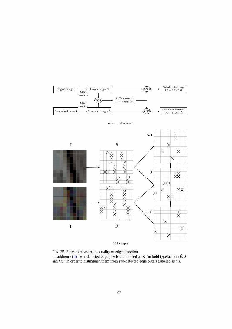
XOR

AND

AND

Edgedetection

Edgedetection

Original imageI

Demosaiced imageI

Original edgesB

Demosaiced edgesB

Sub-detection mapSD= J AND B

Over-detection mapOD = J AND B

Difference mapJ = B XOR B

(a) General scheme

I

I

B

B

SD

OD

J

(b) Example

FIG. 35: Steps to measure the quality of edge detection.In subfigure(b), over-detected edge pixels are labeled as××××××××× (in bold typeface) inB, JandOD, in order to distinguish them from sub-detected edge pixels(labeled as×).

67

SD

OD

SD(X)OD (X)

FIG. 36: ComputingSD andOD from SD andOD, on an example. Pixels labeled asdotted× belong to pairs of shifted edge pixels, and are dropped out inthe final detectionmaps.

4. Compute the rates of sub- and over-detected edge pixels respectively as :

SD% =100XY

Card{

P(x,y) | SDx,y 6= 0}

, (110)

OD% =100XY

Card{

P(x,y) | ODx,y 6= 0}

. (111)

Finally, the rate of erroneously detected edge pixels is expressed asED% =SD% +OD%.

4.5.2. Measurements Based on Shifted EdgesBy visually examining the mapJ in figure 35b, we notice the presence of many

pairs of adjacent edge pixels. In such edge pairs, one pixel is detected inBonly (i.e. sub-detected), and the other one inB only (i.e. over-detected). For example, the mapJof figure 35b presents five pairs of adjacent pixels composed of a sub-detected edgepixel (labeled as×) and an over-detected edge pixel (labeled as× in bold typeface).These cases do not result from a bad edge detection, but from aspatial shift of edgepixels between the original and demosaiced images. A sub-detected (respectively, over-detected) edge pixel is shifted when at least one of its neighbors is an over-detected(respectively, sub-detected) edge pixel. Such pairs of pixels are hereafter calledpairsof shifted (edge) pixels.

In order to characterize the effect of demosaicing on edge detection precisely, wewant to distinguish pairs of shifted edge pixels from other edge pixels. For this pur-pose, we represent unshifted sub- and over-detected edge pixels as two binary mapsrespectively denoted asSDandOD, and defined as :

68

SDx,y 6= 0 ⇔ SDx,y 6= 0∧(6 ∃Q(x′,y′) ∈ N8 (P(x,y))

∣∣ODx′,y′ 6= 0)

, (112)

ODx,y 6= 0 ⇔ ODx,y 6= 0∧(6 ∃Q(x′,y′) ∈ N8 (P(x,y))

∣∣SDx′,y′ 6= 0)

, (113)

where symbol∧ represents the logical AND operator.Figure 36 illustrates, from the example of figure35, how mapsSD and OD are

obtained. In this figure, mapsSDandOD used to buildSDandOD are superimposedin order to highlight the pairs of shifted edge pixels.

From the two binary mapsSD and OD, we compute the rates of sub- and over-detected unshifted edge pixels as :

SD% =100XY

Card{

P(x,y) | SDx,y 6= 0}

, (114)

OD% =100XY

Card{

P(x,y) | ODx,y 6= 0}

. (115)

These rates are used to evaluate precisely the quality of edge detection in demosai-ced images.

4.6. Conclusion

In this section, we have presented the techniques of objective evaluation of demo-saicing quality. For this purpose, we have first presented the most occurred artifactscaused by demosaicing. Blurring, false colors and zipper effect damage the quality ofthe demosaiced images.

Then, we have presented classical criteria which total the errors between the origi-nal and estimated colors through the image. These criteria have some limits since theyprovide a global estimation of the demosaicing quality and do not reflect the judgmentof an observer. Indeed, they do not quantify the occurrencesof artifacts which can beidentified by an observer. Therefore, we have described measurements dedicated tothree kinds of artifacts.

In the computer vision context, most images are acquired by color mono-sensor ca-meras in order to be automatically processed. So, the quality of demosaicing affects thequality of low-level image analysis schemes. That is the reason why we have proposedcriteria which are based on the quality of edge detection.

69

5. Quality Evaluation Results

5.1. Results of Classical Criteria

The quality of demosaicing results, achieved by the ten methods detailed in sec-tion 2, has been first evaluated thanks to classical criteria. For this purpose, the twelvemostly used images of Kodak benchmark database are considered (see figure37)8.These images, all of size 768× 512 pixels, have been selected in order to present asignificant variety of homogeneous regions, colors and textured areas.

Table3 displays the results obtained with criteria which measure the fidelity of eachdemosaiced image to its corresponding original image, namely the mean absolute er-ror (MAE, expression (82)), the peak signal-to-noise ratio (PSNR, expression (85)) andthe correlation criterion (C, expression (87)). Table4 shows, for the same images anddemosaicing schemes, the results obtained with perceptualcriteria, namely the estima-tion error in CIEL∗a∗b∗ color space (∆EL∗a∗b∗ , expression (92)), the estimation errorin S-CIEL∗a∗b∗ color space (∆ES-L∗a∗b∗) and the criterion of normalized color diffe-rence (NCD, expression (97)) between the demosaiced image and its original image.

These two tables show that for a given method, the performances measured witha specific criterion vary from an image to another one. This confirms that obtaininga good color estimation from the CFA image is all the more difficult as the image isrich in high spatial frequency areas. For instance, thePSNRof images demosaiced bybilinear interpolation ranges from 24.5 dB for image 4 (“House”), which contains alot of high frequency areas, to 36 dB for image 1 (“Parrots”),which contains a lot ofhomogeneous regions.

It can be noticed that the two methods which chiefly use the frequency domainprovide better results than those which only scan the spatial domain. Moreover, themethod proposed byDubois(2005) achieves the best average results over the twelveimages, whatever the considered criterion. We also notice that the different criteriaprovide similar performance rankings for the methods on a given image.

5.2. Results of Artifact-sensitive Measurements

5.2.1. Zipper Effect MeasurementsIn order to compare the relevance of the results provided by the two zipper effect

measurements described in section4.4.2, we propose to use the following procedure.First, a ground truth is built for the zipper effect by visually examining the demosaicedimage and defining whether each pixel is affected by zipper effect or not. Then, thetwo measurements are applied, in order to provide binary maps where pixels which areaffected by zipper effect are labeled as white. A final comparison step of these binarymaps with the ground truth quantifies the performance of eachobjective measurement,by counting pixels where zipper effect is correctly detected, sub-detected and over-detected.

Figure38displays the results on four image extracts of size 10×10 pixels. It showsthat the directional alternation measurement generally fits better with the ground truth

8This database is available athttp://www.math.purdue.edu/~lucier/PHOTO_CD

70

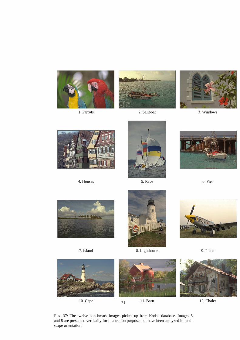
1. Parrots 2. Sailboat 3. Windows

4. Houses 5. Race 6. Pier

7. Island 8. Lighthouse 9. Plane

10. Cape 11. Barn 12. Chalet

FIG. 37: The twelve benchmark images picked up from Kodak database. Images 5and 8 are presented vertically for illustration purpose, but have been analyzed in land-scape orientation.

71

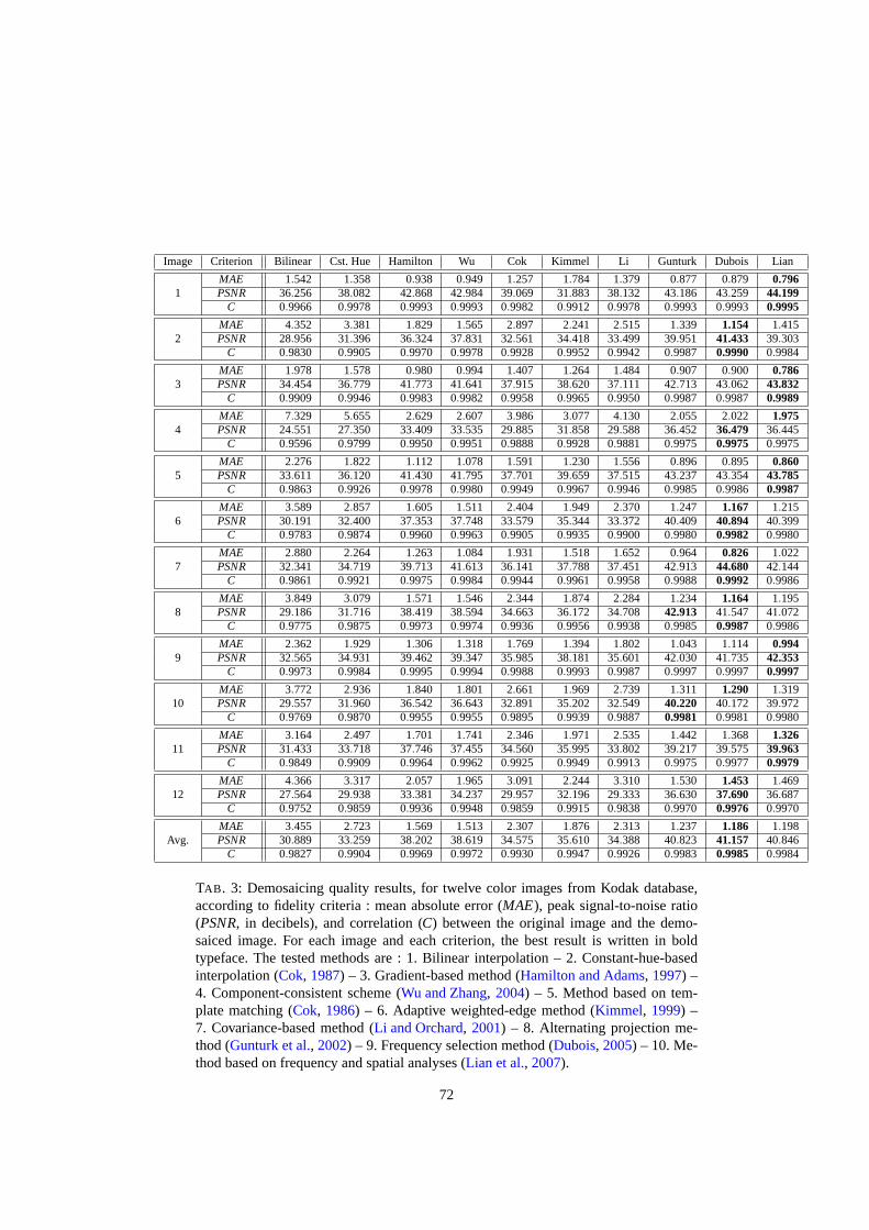
Image Criterion Bilinear Cst. Hue Hamilton Wu Cok Kimmel Li Gunturk Dubois Lian

1MAE 1.542 1.358 0.938 0.949 1.257 1.784 1.379 0.877 0.879 0.796PSNR 36.256 38.082 42.868 42.984 39.069 31.883 38.132 43.186 43.259 44.199

C 0.9966 0.9978 0.9993 0.9993 0.9982 0.9912 0.9978 0.9993 0.9993 0.9995

2MAE 4.352 3.381 1.829 1.565 2.897 2.241 2.515 1.339 1.154 1.415PSNR 28.956 31.396 36.324 37.831 32.561 34.418 33.499 39.951 41.433 39.303

C 0.9830 0.9905 0.9970 0.9978 0.9928 0.9952 0.9942 0.9987 0.9990 0.9984

3MAE 1.978 1.578 0.980 0.994 1.407 1.264 1.484 0.907 0.900 0.786PSNR 34.454 36.779 41.773 41.641 37.915 38.620 37.111 42.713 43.062 43.832

C 0.9909 0.9946 0.9983 0.9982 0.9958 0.9965 0.9950 0.9987 0.9987 0.9989

4MAE 7.329 5.655 2.629 2.607 3.986 3.077 4.130 2.055 2.022 1.975PSNR 24.551 27.350 33.409 33.535 29.885 31.858 29.588 36.452 36.479 36.445

C 0.9596 0.9799 0.9950 0.9951 0.9888 0.9928 0.9881 0.9975 0.9975 0.9975

5MAE 2.276 1.822 1.112 1.078 1.591 1.230 1.556 0.896 0.895 0.860PSNR 33.611 36.120 41.430 41.795 37.701 39.659 37.515 43.237 43.354 43.785

C 0.9863 0.9926 0.9978 0.9980 0.9949 0.9967 0.9946 0.9985 0.9986 0.9987

6MAE 3.589 2.857 1.605 1.511 2.404 1.949 2.370 1.247 1.167 1.215PSNR 30.191 32.400 37.353 37.748 33.579 35.344 33.372 40.409 40.894 40.399

C 0.9783 0.9874 0.9960 0.9963 0.9905 0.9935 0.9900 0.9980 0.9982 0.9980

7MAE 2.880 2.264 1.263 1.084 1.931 1.518 1.652 0.964 0.826 1.022PSNR 32.341 34.719 39.713 41.613 36.141 37.788 37.451 42.913 44.680 42.144

C 0.9861 0.9921 0.9975 0.9984 0.9944 0.9961 0.9958 0.9988 0.9992 0.9986

8MAE 3.849 3.079 1.571 1.546 2.344 1.874 2.284 1.234 1.164 1.195PSNR 29.186 31.716 38.419 38.594 34.663 36.172 34.708 42.913 41.547 41.072

C 0.9775 0.9875 0.9973 0.9974 0.9936 0.9956 0.9938 0.9985 0.9987 0.9986

9MAE 2.362 1.929 1.306 1.318 1.769 1.394 1.802 1.043 1.114 0.994PSNR 32.565 34.931 39.462 39.347 35.985 38.181 35.601 42.030 41.735 42.353

C 0.9973 0.9984 0.9995 0.9994 0.9988 0.9993 0.9987 0.9997 0.9997 0.9997

10MAE 3.772 2.936 1.840 1.801 2.661 1.969 2.739 1.311 1.290 1.319PSNR 29.557 31.960 36.542 36.643 32.891 35.202 32.549 40.220 40.172 39.972

C 0.9769 0.9870 0.9955 0.9955 0.9895 0.9939 0.9887 0.9981 0.9981 0.9980

11MAE 3.164 2.497 1.701 1.741 2.346 1.971 2.535 1.442 1.368 1.326PSNR 31.433 33.718 37.746 37.455 34.560 35.995 33.802 39.217 39.575 39.963

C 0.9849 0.9909 0.9964 0.9962 0.9925 0.9949 0.9913 0.9975 0.9977 0.9979

12MAE 4.366 3.317 2.057 1.965 3.091 2.244 3.310 1.530 1.453 1.469PSNR 27.564 29.938 33.381 34.237 29.957 32.196 29.333 36.630 37.690 36.687

C 0.9752 0.9859 0.9936 0.9948 0.9859 0.9915 0.9838 0.9970 0.9976 0.9970

Avg.MAE 3.455 2.723 1.569 1.513 2.307 1.876 2.313 1.237 1.186 1.198PSNR 30.889 33.259 38.202 38.619 34.575 35.610 34.388 40.823 41.157 40.846

C 0.9827 0.9904 0.9969 0.9972 0.9930 0.9947 0.9926 0.9983 0.9985 0.9984

TAB . 3: Demosaicing quality results, for twelve color images from Kodak database,according to fidelity criteria : mean absolute error (MAE), peak signal-to-noise ratio(PSNR, in decibels), and correlation (C) between the original image and the demo-saiced image. For each image and each criterion, the best result is written in boldtypeface. The tested methods are : 1. Bilinear interpolation – 2. Constant-hue-basedinterpolation (Cok, 1987) – 3. Gradient-based method (Hamilton and Adams, 1997) –4. Component-consistent scheme (Wu and Zhang, 2004) – 5. Method based on tem-plate matching (Cok, 1986) – 6. Adaptive weighted-edge method (Kimmel, 1999) –7. Covariance-based method (Li and Orchard, 2001) – 8. Alternating projection me-thod (Gunturk et al., 2002) – 9. Frequency selection method (Dubois, 2005) – 10. Me-thod based on frequency and spatial analyses (Lian et al., 2007).

72

Image Criterion Bilinear Cst. Hue Hamilton Wu Cok Kimmel Li Gunturk Dubois Lian

1∆EL∗a∗b∗ 1.439 1.289 1.002 1.010 1.229 1.655 1.387 0.969 0.952 0.899

∆ES-L∗a∗b∗ 2.605 2.605 2.318 2.268 2.682 5.701 3.537 2.193 1.967 2.007NCD 0.0098 0.0089 0.0067 0.0068 0.0083 0.0119 0.0094 0.0064 0.0064 0.0060

2∆EL∗a∗b∗ 3.382 2.562 1.538 1.335 2.275 1.772 2.078 1.196 1.078 1.223

∆ES-L∗a∗b∗ 6.477 5.965 3.756 2.954 5.360 4.653 4.578 3.079 2.440 3.021NCD 0.0251 0.0194 0.0113 0.0099 0.0169 0.0136 0.0152 0.0089 0.0079 0.0091

3∆EL∗a∗b∗ 2.048 1.663 1.132 1.148 1.492 1.491 1.653 1.108 1.066 0.981

∆ES-L∗a∗b∗ 3.715 3.483 2.659 2.615 3.339 4.283 3.990 2.594 2.280 2.229NCD 0.0140 0.0114 0.0077 0.0078 0.0101 0.0102 0.0112 0.0074 0.0072 0.0066

4∆EL∗a∗b∗ 5.467 4.246 2.167 2.099 3.138 2.356 3.315 1.735 1.676 1.652

∆ES-L∗a∗b∗ 11.293 10.635 5.729 5.166 7.918 6.125 7.886 4.850 4.507 4.327NCD 0.0441 0.0338 0.0172 0.0169 0.0249 0.0193 0.0261 0.0140 0.0136 0.0132

5∆EL∗a∗b∗ 1.780 1.474 0.965 0.931 1.273 1.040 1.299 0.861 0.843 0.816

∆ES-L∗a∗b∗ 3.925 3.824 2.753 2.661 3.401 3.462 3.344 2.437 2.361 2.304NCD 0.0139 0.0114 0.0074 0.0072 0.0099 0.0082 0.0100 0.0065 0.0064 0.0062

6∆EL∗a∗b∗ 3.511 2.762 1.729 1.641 2.419 1.943 2.485 1.393 1.334 1.343

∆ES-L∗a∗b∗ 6.883 6.417 4.333 3.809 5.781 4.806 5.675 3.589 3.209 3.323NCD 0.0261 0.0209 0.0128 0.0122 0.0179 0.0151 0.0183 0.0104 0.0099 0.0100

7∆EL∗a∗b∗ 2.671 2.047 1.259 1.088 1.789 1.407 1.592 1.021 0.895 1.051

∆ES-L∗a∗b∗ 5.231 4.808 3.135 2.496 4.254 3.563 3.580 2.597 1.991 2.635NCD 0.0206 0.0161 0.0096 0.0083 0.0138 0.0113 0.0121 0.0079 0.0068 0.0081

8∆EL∗a∗b∗ 3.338 2.629 1.561 1.526 2.170 1.806 2.195 1.260 1.188 1.224

∆ES-L∗a∗b∗ 6.474 5.984 3.811 3.465 5.039 4.404 4.857 3.208 2.860 2.963NCD 0.0243 0.0193 0.0111 0.0110 0.0156 0.0133 0.0157 0.0090 0.0085 0.0087

9∆EL∗a∗b∗ 2.155 1.725 1.221 1.208 1.613 1.277 1.709 0.996 1.005 0.959

∆ES-L∗a∗b∗ 4.568 4.136 3.175 2.984 3.909 3.346 4.663 2.791 2.697 2.478NCD 0.0150 0.0122 0.0086 0.0086 0.0113 0.0093 0.0119 0.0071 0.0072 0.0068

10∆EL∗a∗b∗ 3.259 2.524 1.705 1.652 2.356 1.696 2.517 1.273 1.261 1.278

∆ES-L∗a∗b∗ 6.239 5.839 4.234 3.826 5.555 4.060 5.694 3.321 3.107 3.140NCD 0.0251 0.0197 0.0131 0.0128 0.0182 0.0137 0.0192 0.0099 0.0097 0.0098

11∆EL∗a∗b∗ 2.724 2.152 1.584 1.602 2.065 1.822 2.284 1.416 1.319 1.303

∆ES-L∗a∗b∗ 5.175 4.747 3.898 3.738 4.852 4.690 5.371 3.631 3.157 3.191NCD 0.0195 0.0157 0.0114 0.0116 0.0149 0.0133 0.0165 0.0101 0.0095 0.0093

12∆EL∗a∗b∗ 3.402 2.620 1.736 1.655 2.482 1.814 2.730 1.380 1.318 1.317

∆ES-L∗a∗b∗ 6.286 5.870 4.341 3.920 5.965 4.384 6.371 3.564 3.135 3.193NCD 0.0258 0.0200 0.0132 0.0127 0.0188 0.0142 0.0206 0.0105 0.0101 0.0100

Avg.∆EL∗a∗b∗ 2.931 2.308 1.467 1.408 2.025 1.673 2.104 1.217 1.161 1.170

∆ES-L∗a∗b∗ 5.739 5.359 3.678 3.325 4.838 4.456 4.962 3.154 2.809 2.901NCD 0.0219 0.0174 0.0108 0.0105 0.0150 0.0128 0.0155 0.0090 0.0086 0.0086

TAB . 4: Demosaicing quality results, for twelve color images from Kodak database,according to perceptual criteria : estimation error in CIEL∗a∗b∗ color space (∆EL∗a∗b∗),estimation error in S-CIEL∗a∗b∗ color space (∆ES-L∗a∗b∗ ), and criterion of normalizedcolor difference (NCD). For each image and each criterion, the best result (i.e. lowestvalue) is written in bold typeface. Images and tested methods are the same as in table3.The illuminant used for(X,Y,Z) transform is the standard CIE D65, which correspondsto daylight.

73

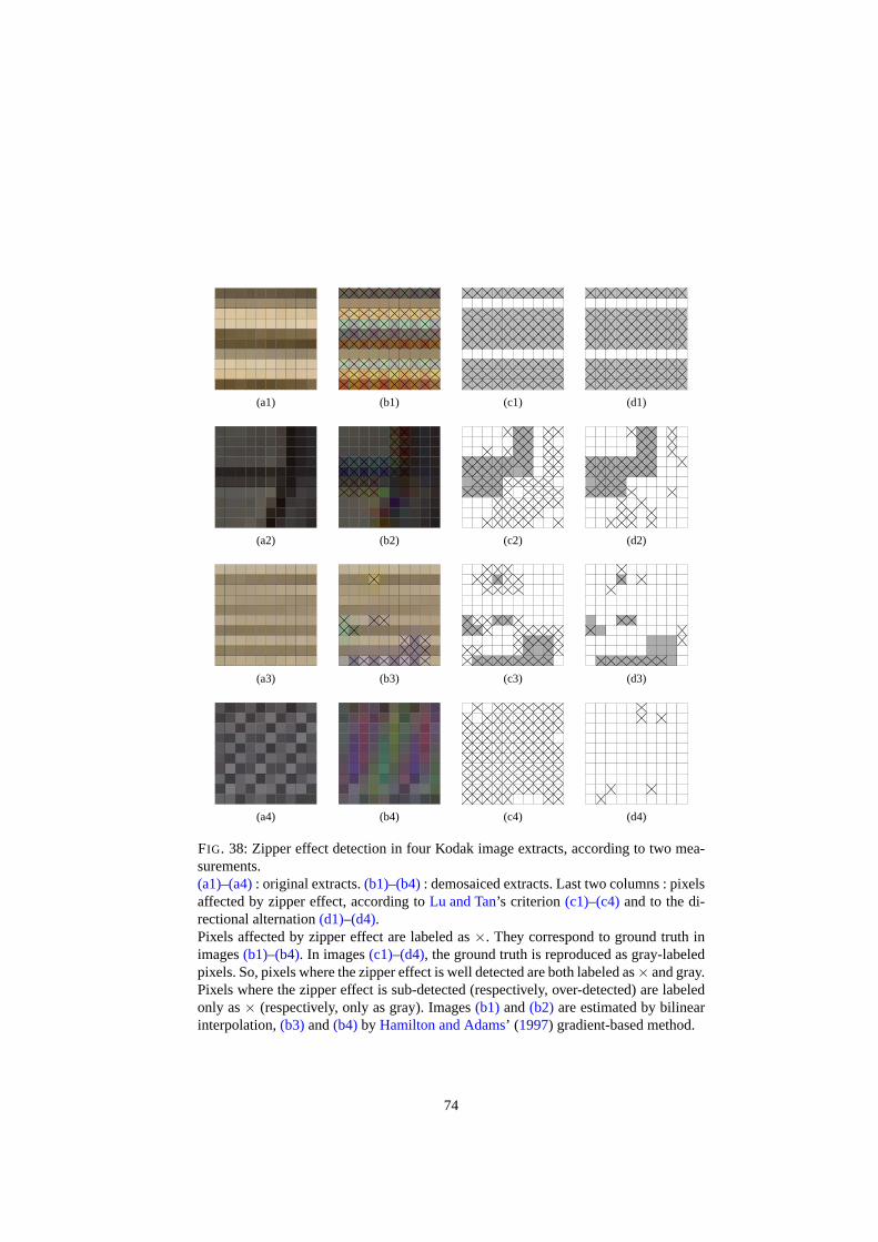
(a1) (b1) (c1) (d1)

(a2) (b2) (c2) (d2)

(a3) (b3) (c3) (d3)

(a4) (b4) (c4) (d4)

FIG. 38: Zipper effect detection in four Kodak image extracts, according to two mea-surements.(a1)–(a4): original extracts.(b1)–(b4) : demosaiced extracts. Last two columns : pixelsaffected by zipper effect, according toLu and Tan’s criterion (c1)–(c4) and to the di-rectional alternation(d1)–(d4).Pixels affected by zipper effect are labeled as×. They correspond to ground truth inimages(b1)–(b4). In images(c1)–(d4), the ground truth is reproduced as gray-labeledpixels. So, pixels where the zipper effect is well detected are both labeled as× and gray.Pixels where the zipper effect is sub-detected (respectively, over-detected) are labeledonly as× (respectively, only as gray). Images(b1) and(b2) are estimated by bilinearinterpolation,(b3)and(b4)by Hamilton and Adams’ (1997) gradient-based method.

74

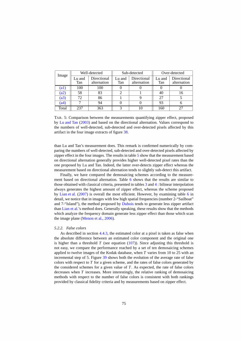
ImageWell-detected Sub-detected Over-detected

Lu andTan

Directionalalternation

Lu andTan

Directionalalternation

Lu andTan

Directionalalternation

(a1) 100 100 0 0 0 0(a2) 58 83 2 1 40 16(a3) 72 86 1 9 27 5(a4) 7 94 0 0 93 6Total 237 363 3 10 160 27

TAB . 5: Comparison between the measurements quantifying zipper effect, proposedby Lu and Tan(2003) and based on the directional alternation. Values correspond tothe numbers of well-detected, sub-detected and over-detected pixels affected by thisartifact in the four image extracts of figure38.

than Lu and Tan’s measurement does. This remark is confirmed numerically by com-paring the numbers of well-detected, sub-detected and over-detected pixels affected byzipper effect in the four images. The results in table5 show that the measurement basedon directional alternation generally provides higher well-detected pixel rates than theone proposed by Lu and Tan. Indeed, the latter over-detects zipper effect whereas themeasurement based on directional alternation tends to slightly sub-detect this artifact.

Finally, we have compared the demosaicing schemes according to the measure-ment based on directional alternation. Table6 shows that the results are similar tothose obtained with classical criteria, presented in tables3 and4 : bilinear interpolationalways generates the highest amount of zipper effect, whereas the scheme proposedby Lian et al.(2007) is overall the most efficient. However, by examining table6 indetail, we notice that in images with few high spatial frequencies (number 2-“Sailboat”and 7-“Island”), the method proposed byDuboistends to generate less zipper artifactthanLian et al.’s method does. Generally speaking, these results show thatthe methodswhich analyze the frequency domain generate less zipper effect than those which scanthe image plane (Menon et al., 2006).

5.2.2. False colorsAs described in section4.4.3, the estimated color at a pixel is taken as false when

the absolute difference between an estimated color component and the original oneis higher than a thresholdT (see equation (107)). Since adjusting this threshold isnot easy, we compare the performance reached by a set of ten demosaicing schemesapplied to twelve images of the Kodak database, whenT varies from 10 to 25 with anincremental step of 5. Figure39 shows both the evolution of the average rate of falsecolors with respect toT for a given scheme, and the rates of false colors generated bythe considered schemes for a given value ofT. As expected, the rate of false colorsdecreases whenT increases. More interestingly, the relative ranking of demosaicingmethods with respect to the number of false colors is consistent with both rankingsprovided by classical fidelity criteria and by measurementsbased on zipper effect.

75

Image Bilinear Cst. Hue Hamilton Wu Cok Kimmel Li Gunturk Dubois Lian1 4.317 1.939 0.623 0.822 0.735 4.408 3.068 0.893 0.861 0.3452 22.567 12.761 2.656 2.082 4.903 2.464 7.157 0.682 0.487 0.5903 8.793 4.581 1.257 1.626 1.374 1.795 4.093 1.664 1.278 0.5464 35.932 25.164 4.485 5.393 7.214 5.023 14.031 2.402 2.351 1.6105 9.023 4.226 0.610 0.581 1.110 0.658 2.069 0.664 0.482 0.1926 19.876 10.707 2.955 3.405 3.986 2.797 7.868 1.562 1.441 0.8267 18.483 10.124 1.954 1.213 3.730 1.990 4.579 0.391 0.177 0.4368 18.216 11.672 2.369 3.051 3.811 2.122 7.213 0.850 0.727 0.6179 9.459 5.618 1.695 2.192 2.367 1.537 5.335 0.714 0.709 0.422

10 15.425 9.976 3.021 3.473 4.003 2.475 8.548 0.984 0.967 0.68511 12.816 6.331 1.809 2.726 2.840 1.835 7.083 1.166 0.962 0.51012 18.729 10.107 2.735 3.461 3.761 2.269 9.256 1.285 1.076 0.803

Avg. 16.136 9.434 2.181 2.502 3.319 2.448 6.692 1.105 0.960 0.632

TAB . 6: RatesZE% of pixels affected by zipper effect, according to the measurementbased on directional alternation. The images and tested methods are the same as intable3.

0

2

4

6

8

01

21

41

61

81

02

52025101

T

raeniliB

euH .tsC

notlimaH

uW

koC

lemmiK

iL

krutnuG

siobuD

naiL

FC

%

FIG. 39: Average rates of false colorsFC% with respect to the detection thresholdT.The twelve considered images and ten tested methods are the same as in table3.

76

5.3. Discussion

The most widely used criteria for the evaluation of demosaicing quality areMSEandPSNR, the latter being a logarithmic form of theMSE criterion. Several reasonsexplain why most of the authors use these criteria (Wang and Bovik, 2006). First, thesefunctions are easy to be implemented and their derivatives can be estimated. They maytherefore be integrated into an optimization scheme. Second, thePSNRcriterion has areal physical meaning – namely, the maximal energy of the signal with respect to errorsgenerated by demosaicing –, which can also be analyzed in thefrequency domain.

However, thePSNRcriterion provides a general estimation of the demosaicingqua-lity, but does not really reflect the human judgment. For example, an observer wouldprefer an image containing a large number of pixels with estimated colors close tothe original ones, than an image containing a reduced numberof pixels affected by vi-sible artifacts. ButMSEandPSNRcriteria could provide identical values in both cases,since they do not discriminate the characteristics of different artifacts in the demosaicedimage. These objective measurements have been criticized (Wang and Bovik, 2009)since they cannot evaluate the image alteration as a human observer does (Eskicioglu and Fisher,1995).

The alternative criteria∆E of estimation errors in the CIEL∗a∗b∗ and S-CIEL∗a∗b∗

color spaces are the most widely used perceptual criteria (Zhang and Wandell, 1997).They are based on perceptually uniform color spaces as an attempt to represent thehuman perception, but require prior knowledge about the illuminant and the referencewhite used during image acquisition. Since the acquisitionconditions are not alwaysknown, the quality of these measurements may be biased.

5.4. Experimental Results for Edge Detection

The demosaicing performance has been evaluated with respect to the quality ofedge detection thanks to measurements detailed in section4.5. Table7 displays theaverage rates of sub-detected (SD%), over-detected (OD%) and erreneously detected(ED% = SD% +OD%) edge pixels. These values have been computed over the twelveKodak images previously considered, and for the ten classical demosaicing schemes.Moreover, this table displays the average ratesSD%, OD% andED% which take into ac-count only unshifted edge pixels. The lowest values correspond to the best demosaicingquality according to these edge-dedicated measurements.

By examining the average ratesED% andED%, similar conclusions can be drawnabout the performances of demosaicing schemes. The methodswhich privilege thefrequency domain allow to obtain better edge detection quality than the other methodsdo. Besides, the methods proposed byDubois and byLian et al.provide the lowesterror rates in both edge and unshifted edge detection. Thesedemosaicing schemes aretherefore the most apt to be coupled with edge detection procedures based on colorgradient.

Moreover, we notice that the ranking of the ten tested demosaicing schemes withrespect toOD% andSD% is relatively consistent with the ranking obtained with mea-surementsOD% and SD%. However, the rate of over-detected unshifted pixels is thelowest for bilinear interpolation. This suprising performance result can be explained

77

Meas. Bilinear Cst. Hue Hamilton Wu Cok Kimmel Li Gunturk Dubois Lian

SD% 3.673 2.090 1.528 1.561 1.882 1.983 2.265 1.422 1.278 1.323

OD% 2.257 1.945 1.504 1.522 1.818 1.802 2.319 1.242 1.199 1.263

ED% 5.930 4.035 3.032 3.083 3.700 3.785 4.584 2.664 2.477 2.586

SD% 1.945 1.109 0.881 0.877 1.032 1.077 1.094 0.888 0.774 0.803

OD% 0.663 0.979 0.855 0.842 0.974 0.912 1.156 0.713 0.697 0.748

ED% 2.608 2.088 1.736 1.719 2.006 1.989 2.250 1.601 1.471 1.551

TAB . 7: Average rates of sub-detected edge pixels (SD%), of over-detected edge pixels(OD%) and erreneously detected pixels (ED% = SD% + OD%). Average rates of sub-detected unshifted edge pixels (SD%), of over-detected unshifted edge pixels (OD%)and of unshifted edge pixels that are erreneously detected (ED% = SD% + OD%). Thelow and high thresholds used for hysteresis thresholding are set to 1 and 6, respectively.The twelve considered images and ten tested methods are the same as in table3.

by both strong blurring and zipper effect generated by this demosaicing method. In-deed, blurring induces fewer detected edge pixels, and zipper effect mainly inducespairs of shifted edge pixels.

For each of the other methods, the rates of sub- and over-detected edge pixels areoverall similar. Moreover, their ranking is almost the sameas the one obtained with theprevious criteria.

In table7, we also notice that more than the half of sub- and over-detected edgepixels according to measurementsSD% and OD% are not retrieved with measure-mentsSD% and OD%. That means that shifted edges strongly contribute to the dis-similarity between edges detected in the original and demosaiced images.

Edge pixels are sub-detected because the color gradient module used to detect edgesdecreases with blurring in demosaiced images. The over-detected edge pixels corres-pond to an increase of the color gradient module in case of zipper effect or false colors.These new rates of sub- and over-detected pixelsSD% and OD% are able to reflectthe artifacts caused by demosaicing. From table7, we can evaluate the influence, onedge detection, of the demosaicing strategies implementedin the tested methods. Bothmethods using bilinear interpolation and hue constancy estimate the pixel colors wi-thout exploiting spatial correlation. Hence, they generate more artifacts than the threeother methods which exploit spatial correlation, and provide higher rates of sub- andover-detected edge pixels.

All in all, sub- and over-detected edge pixels often coincide with artifacts. Figure40shows images which are demosaiced by two different schemes,and the respective mapsof sub- and over-detected unshifted edge pixels (SDandOD). We notice that demosai-cing influences the edge detection more significantly in areas with high spatial frequen-cies and that the artifacts are also mainly located in these areas.

Zipper effect often decreases the variation of levels in transition areas betweenhomogeneous regions. Hence, zipper effect tends to decrease the gradient module, sothat the norm of local maxima becomes lower than the high thresholdTh used by the

78

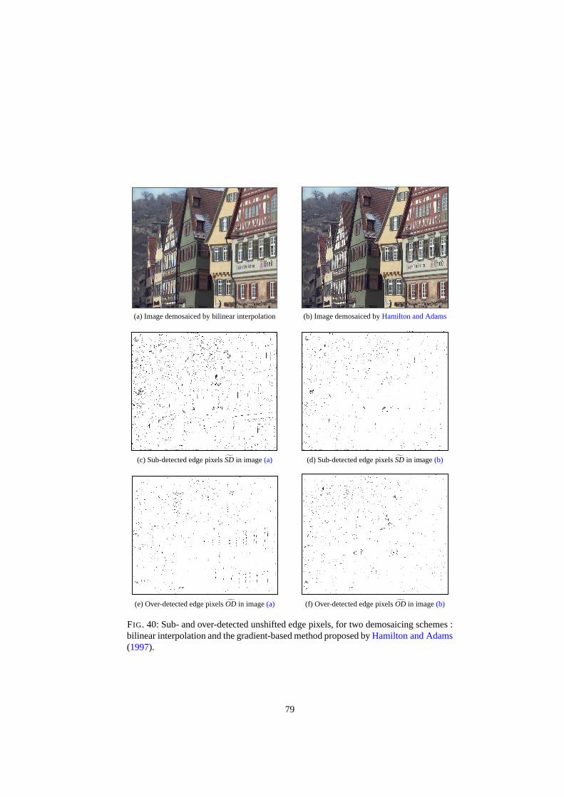
(a) Image demosaiced by bilinear interpolation (b) Image demosaiced byHamilton and Adams

(c) Sub-detected edge pixelsSD in image(a) (d) Sub-detected edge pixelsSD in image(b)

(e) Over-detected edge pixelsOD in image(a) (f) Over-detected edge pixelsOD in image(b)

FIG. 40: Sub- and over-detected unshifted edge pixels, for two demosaicing schemes :bilinear interpolation and the gradient-based method proposed byHamilton and Adams(1997).

79

(a) Original imageI (b) Demosaiced imageI (c) Comparison between detected edgepixels (green : coinciding ; blue : sub-

detected ; red : over-detected)

FIG. 41: Example of edge pixels which are not modified by pixels affected by false co-lors, on an image demosaiced by the scheme proposed byHamilton and Adams(1997).

hysteresis thresholding (see page65). This explains why zipper effect causes edge sub-detection. Since a lot of pixels are affected by zipper effect, the rate of sub-detectededge pixels is generally lower than that of over-detected ones.

Isolated pixels affected by false colors do not always change the location of detec-ted edge pixels. Figure41shows that pixels affected with false colors do not change thequality of edge detection, on an extract of the image “Houses”. At these pixels indeed,the gradient module increases, whereas the location of edgepixels remains unchanged.

On the other hand, when the local density of pixels affected by false colors is high,they cause edge over-detection. In textured areas with thindetails, most demosaicingschemes generate a lot of neighboring pixels affected by false colors. The gradient mo-dule at these pixels increases since its computation takes into account several neigh-boring false colors. The gradient module at local maxima increases, so that it maybecome higher than the high thresholdTh used by the hysteresis thresholding. In thatcase, new edge pixels are detected. For example, figure40 shows that edge pixels areover-detected in textured areas which correspond to the shutters and to the tiles of thehouse roofs.

Finally, we notice that statistics about sub-detected edgepixels can be exploited tomeasure the blurring effect caused by demosaicing, and thatover-detected pixels arelocated in areas with a high density of false colors.

80

6. Conclusion

This paper is related to the majority of digital color cameras, which are equippedwith a single sensor. The surface of this sensor is covered bya color filter array whichconsists in a mosaic of spectrally selective filters, so thateach sensor element samplesonly one of the three color components Red, Green or Blue. We focus on the BayerCFA which is the most widely used. To estimate the color (R,G,B) of each pixel ina true color image, one has to determine the values of the two missing color compo-nents at each pixel in the CFA image. This process is commonlyreferred to asCFAdemosaicing, and its result as thedemosaiced image.

Demosaicing methods may exploit the spatial and/or frequency domains. The spa-tial domain has been historically used first, and many methods are based on assump-tions about spectral and/or spatial correlation. More recently, works have appeared thatexploit the frequency domain, which opens wide perspectives.

We have compared the performances reached by ten demosaicing schemes appliedto twelve images extracted from Kodak database, with respect to three kinds of qualitymeasurements : classical fidelity criteria, artifact-sensitive measurements and measu-rements dedicated to edge detection. The rankings between the demosaicing schemesestablished thanks to these measurements are consistent.

This detailed evaluation highlights that the methods whichprimarily analyze thefrequency domain outperform those which only scan the spatial domain. More preci-sely, the methods proposed byDubois(2005) and byLian et al.(2007) provide the bestdemosaicing results whatever the criterion used.

The implementation of demosaicing schemes has to respect real-time constraints.Indeed, the time required for image demosaicing has to be lower than the image acqui-sition time. Hence, it would be useful to look for a compromise between the processingtime and the performance reached by the examined demosaicing schemes. This studywould allow to select the best methods which are less time-consuming.

Thanks to a visual comparison of the results, we have described the relationshipsbetween artifacts and edge detection quality. Zipper effect causes edge sub-detection,whereas a high density of pixels affected with false colors tends to cause over-detectionof edge pixels. These preliminary conclusions are worth being generalized to the rela-tionships between artifacts and the detection quality of other features in the demosaicedimages.

81

Alleysson, D., Chaix de Lavarène, B., Süsstrunk, S., Hérault, J., Sep. 2008. LinearMinimum Mean Square Error Demosaicking. CRC Press, Ch. 8, pp. 213–237.

Alleysson, D., Süsstrunk, S., Hérault, J., Apr. 2005. Linear demosaicing inspired bythe human visual system. IEEE Transactions on Image Processing 14 (4), 439–449.

Astola, J., Haavisto, P., Neuvo, Y., Apr. 1990. Vector median filters. Proceedings of theIEEE 78 (4), 678–689.

Asuni, N., Giachetti, A., Jan. 2008. Accuracy improvementsand artifacts removal inedge-based image interpolation. In : Ranchordas, A., Araújo, H. (Eds.), Proceedingsof the 3rd International Conference on Computer Vision Theory and Application(VISAPP’08). Funchal, Madeira, Portugal, pp. 58–65.

Bayer, B. E., Jul. 1976. Color imaging array. U.S. patent 3,971,065, to Eastman KodakCo., Patent and Trademark Office, Washington D.C.

Bayrama, S., Sencar, H. T., Memon, N., Sep. 2008. Classification of digital camera-models based on demosaicing artifacts. Digital Investigation 5 (1-2), 49–59.

Buades, A., Coll, B., Morel, J.-M., Sbert, C., Aug. 2008. Nonlocal demosaicing. In :Proceedings of the 2008 International Workshop on Local andNon-Local Approxi-mation in Image Processing (LNLA’08). Lausanne, Suisse.

Busin, L., Vandenbroucke, N., Macaire, L., 2008. Color spaces and image segmenta-tion. Advances in Imaging and Electron Physics 151, 65–168.

Chang, L., Tan, Y.-P., Jan. 2006. Hybrid color filter array demosaicking for effectiveartifact suppression. Journal of Electronic Imaging 15 (1), 013003,1–17.

Chen, L., Yap, K.-H., He, Y., Mar. 2008. Subband synthesis for color filter array demo-saicking. IEEE Transactions on Systems, Man and Cybernetics 38 (2), 485–492.

Chung, K.-H., Chan, Y.-H., Oct. 2006. Color demosaicing using variance of color dif-ferences. IEEE Transactions on Image Processing 15 (10), 2944–2955.

Cok, D. R., Dec. 1986. Signal processing method and apparatus for sampled imagesignals. U.S. patent 4,630,307, to Eastman Kodak Co., Patent and Trademark Office,Washington D.C.

Cok, D. R., Feb. 1987. Signal processing method and apparatus for producing interpo-lated chrominance values in a sampled color image signal. U.S. patent 4,642,678, toEastman Kodak Co., Patent and Trademark Office, Washington D.C.

Cok, D. R., May 1994. Reconstruction of CCD images using template matching. In :Proceedings of the IS&T’s 47th Annual Conference, Physics and Chemistry of Ima-ging Systems (ICPS’94). Vol. 2. Rochester, New York, U.S.A., pp. 380–385.

Condat, L., Nov. 2009. A new random color filter array with good spectral proper-ties. In : Proceedings of the IEEE International Conferenceon Image Processing(ICIP’09). Cairo, Egypt [to appear].

82

Deriche, R., May 1987. Using Canny’s criteria to derive a recursively implementedoptimal edge detector. The International Journal of Computer Vision 1 (2), 167–187.

Di Zenzo, S., Jan. 1986. A note on the gradient of a multi-image. Computer Vision,Graphics, and Image Processing 33 (1), 116–125.

Dubois, E., Dec. 2005. Frequency-domain methods for demosaicking of Bayer-sampled color images. IEEE Signal Processing Letters 12 (12), 847–850.

Eastman Kodak and various photographers, 1991. Kodak PhotoCD PCD0992, AccessSoftware & Photo Sampler, Final version 2.0. [CD-ROM, Part No. 15-1132-01].

Eskicioglu, A. M., Fisher, P. S., Dec. 1995. Image quality measures and their perfor-mance. IEEE Transactions on Communications 43 (12), 2959–2965.

Faugeras, O. D., Aug. 1979. Digital color image processing within the framework of ahuman visual model. IEEE Transactions on Acoustics, Speech, and Signal Proces-sing 27 (4), 380–393.

Freeman, W. T., Dec. 1988. Median filter for reconstructing missing color samples.U.S. patent 4,724,395, to Polaroid Co., Patent and Trademark Office, WashingtonD.C.

Gribbon, K. T., Bailey, D. G., Jan. 2004. A novel approach to real-time bilinear in-terpolation. In : Proceedings of the 2nd IEEE InternationalWorkshop on ElectronicDesign, Test and Applications (DELTA’04). Perth, Australia, pp. 126–131.

Gunturk, B. K., Altunbasak, Y., Mersereau, R. M., Sep. 2002.Color plane interpolationusing alternating projections. IEEE Transactions on ImageProcessing 11 (9), 997–1013.

Gunturk, B. K., Glotzbach, J., Altunbasak, Y., Schafer, R. W., Mersereau, R. M., Jan.2005. Demosaicking : Color filter array interpolation. IEEESignal Processing Ma-gazine 22 (1), 44–54.

Hamilton, J. F., Adams, J. E., May 1997. Adaptive color plan interpolation in singlesensor color electronic camera. U.S. patent 5,629,734, to Eastman Kodak Co., Patentand Trademark Office, Washington D.C.

Hamilton, J. F., Compton, J. T., Feb. 2007. Processing colorand panchromatic pixels.U.S. Patent 0,024,879 A1, to Eastman Kodak Co., Patent and Trademark Office,Washington D.C.

Harris, C. J., Stephens, M., Aug. 1988. A combined corner andedge detector. In : Pro-ceedings of the 4th Alvey Vision Conference (AVC’88). Manchester, United King-dom, pp. 147–151.

Hibbard, R. H., 1995. Apparatus and method for adaptively interpolating a full colorimage utilizing luminance gradients. U.S. patent 5,382,976, to Eastman Kodak Co.,Patent and Trademark Office, Washington D.C.

83

Hirakawa, K., Sep. 2008. Color filter array image analysis for joint denoising and de-mosaicking. In : Lukac, R. (Ed.), Single-Sensor Imaging : Methods and Applicationsfor Digital Cameras. CRC Press, pp. 239–261.

Hirakawa, K., Parks, T. W., Mar. 2005. Adaptive homogeneity-directed demosaicingalgorithm. IEEE Transactions on Image Processing 14 (3), 360–369.

Jai Corporation, 2000. CV-S3200/S3300 series – Super sensitive DSP color camera(JAI CV-S3300P brochure).http://www.graftek.com/pdf/Brochures/JAI/cv-s3200_3300.pdf.

Kimmel, R., Sep. 1999. Demosaicing : image reconstruction from color CCD samples.IEEE Transactions on Image Processing 8 (9), 1221–1228.

Kröger, R. H. H., Aug. 2004. Anti-aliasing in image recording and display hardware :lessons from nature. Journal of Optics A : Pure and Applied Optics 6, 743U748.

Kuno, T., Sugiura, H., Mar. 2006. Imaging apparatus and mobile terminal incorporatingsame. U.S. Patent 7,019,774 B2, to Mitsubishi Denki Kabushiki Kaisha, Patent andTrademark Office, Washington D.C.

Laroche, C. A., Prescott, M. A., Jun. 1993. Apparatus and method for adaptively inter-polating a full color image utilizing chrominance gradients. U.S. patent 5,373,322,to Eastman Kodak Co., Patent and Trademark Office, Washington D.C.

Leitão, J. A., Zhao, M., de Haan, G., Jan. 2003. Content-adaptive video up-scalingfor high definition displays. In : Proceedings of the SPIE Conference on Image andVideo Communications and Processing (IVCP’03). Santa Clara, California, U.S.A.,pp. 612–622.

Li, J. J., Randhawa, S., Sep. 2005. High order extrapolationusing Taylor series forcolor filter array demosaicing. In : Proceedings of the International Conference onImage Analysis and Recognition (ICIAR’05). Vol. 3656 of Lecture Notes in Com-puter Science. Springer, Berlin-Heidelberg, Toronto, Canada, pp. 703–711.

Li, X., Nov. 2000. Edge directed statistical inference and its applications to imageprocessing. PhD thesis, Princeton University, New Jersey,U.S.A.

Li, X., Mar. 2005. Demosaicing by successive approximation. IEEE Transactions onImage Processing 14 (3), 370–379.

Li, X., Orchard, M. T., Oct. 2001. New edge-directed interpolation. IEEE Transactionson Image Processing 10 (10), 1521–1527.

Lian, N., Chang, L., Tan, Y.-P., Sep. 2005. Improved color filter array demosaicking byaccurate luminance estimation. In : Proceedings of the 12thInternational Conferenceon Image Processing (ICIP’2005). Vol. 1. Genova, Italia, pp. I–41–4.

Lian, N.-X., Chang, L., Tan, Y.-P., Zagorodnov, V., Oct. 2007. Adaptive filtering forcolor filter array demosaicking. IEEE Transactions on ImageProcessing 16 (10),2515–2525.

84

Lian, N.-X., Chang, L., Zagorodnov, V., Tan, Y.-P., Nov. 2006. Reversing demosaickingand compression in color filter array image processing : Performance analysis andmodeling. IEEE Transactions on Image Processing 15 (11), 3261–3278.

Lu, W., Tan, Y.-P., Oct. 2003. Color filter array demosaicking : New method and per-formance measures. IEEE Transactions on Image Processing 12 (10), 1194–1210.

Lu, Y. M., Karzand, M., Vetterli, M., Jan. 2009. Iterative demosaicking accelerated :Theory and fast noniterative implementations. In : Bouman,C. A., Miller, E. L.,Pollak, I. (Eds.), Procs. 21th IS&T/SPIE Electronic Imaging Annual Symposium(SPIE’09). Vol. 7246 of Computational Imaging VII. San Jose, California, USA, pp.72460L–72460L–12.

Lukac, R., Sep. 2008. Single-Sensor Imaging : Methods and Applications for Digi-tal Cameras. Image Processing Series. CRC Press / Taylor & Francis, Boca Raton,Florida, USA.

Lukac, R., Plataniotis, K. N., May 2004a. Normalized color-ratio modeling for CFAinterpolation. IEEE Transactions on Consumer Electronics50 (2), 737–745.

Lukac, R., Plataniotis, K. N., Oct. 2004b. A normalized model for color-ratio baseddemosaicking schemes. In : Proceedings of the 11th International Conference onImage Processing (ICIP’04). Singapore, pp. 1657–1660.

Lukac, R., Plataniotis, K. N., Nov. 2005a. Color filter arrays : Design and performanceanalysis. IEEE Transactions on Consumer Electronics 51 (4), 1260–1267.

Lukac, R., Plataniotis, K. N., Apr. 2005b. Universal demosaicking for imaging pipe-lines with an RGB color filter array. Pattern Recognition 38,2208–2212.

Lukac, R., Plataniotis, K. N., 2007. Single-sensor camera image processing. In : Lukac,R., Plataniotis, K. N. (Eds.), Color Image Processing : Methods and Applications.CRC Press / Taylor & Francis, pp. 363–392.

Lukac, R., Plataniotis, K. N., Hatzinakos, D., Aleksic, M.,Jul. 2006. A new CFA inter-polation framework. Signal Processing 86 (7), 1559–1579.

Lukin, A., Kubasov, D., Sep. 2004. An improved demosaicing algorithm. In : Pro-ceedings of the 14th International Conference on Computer Graphics, GRAPHI-CON’04. Moscow, Russia, pp. 38–45.

Lyon, R., Hubel, P. M., Nov. 2002. Eyeing the camera : into thenext century. In :Proceedings of the 10th Color Imaging Conference (CIC’2002) : Color Science andEngineering Systems, Technologies, Applications. Scottsdale, Arizona, U.S.A., pp.349–355.

Lyon, R. F., Mar. 2000. Prism-based color separation for professional digital photogra-phy. In : Proceedings of the IS&T Conference on Image Processing, Image Quality,Image Capture, Systems (PICS’00). Vol. 3. Portland, Oregon, USA, pp. 50–54.

85

Martin, D. R., Fowlkes, C., Malik, J., May 2004. Learning to detect natural imageboundaries using local brightness, color, and texture cues. IEEE Transactions onPattern Analysis and Machine Intelligence 26 (5), 530–549.

Marziliano, P., Dufaux, F., Winkler, S., Ebrahimi, T., 2004. Perceptual blur and ringingmetrics : application to JPEG2000. Signal Processing : Image Communication 19,163–172.

Medjeldi, T., Horé, A., Ziou, D., Jul. 2009. Enhancement of the quality of imagesthrough complex mosaic configurations. In : Kamel, M., Campilho, A. (Eds.),Proceedings of the International Conference on Image Analysis and Recognition(ICIAR’09). Vol. 5627. Springer, Berlin-Heidelberg, Halifax, Canada, pp. 43–53.

Menon, D., Andriani, S., Calvagno, G., Sep. 2006. A novel technique for reducingdemosaicing artifacts. In : Proceedings of the XIVth European Signal ProcessingConference (EUSIPCO’06). Firenze, Italia.

Menon, D., Andriani, S., Calvagno, G., Jan. 2007. Demosaicing with directional fil-tering anda posteriori decision. IEEE Transactions on Image Processing 16 (1),132–141.

Mukherjee, J., Parthasarathi, R., Goyal, S., Mar. 2001. Markov random field processingfor color demosaicing. Pattern Recognition Letters 22 (3-4), 339–351.

Muresan, D. D., Luke, S., Parks, T. W., Aug. 2000. Reconstruction of color images fromCCD arrays. In : Proceedings of the Texas Instruments Digital Signal ProcessingSystems Fest. Houston, Texas, U.S.A., pp. 1–6 [CD–ROM XP002243635].

Noble, S. A., 2000. The technology inside the new Kodak Professional DCS 620x digi-tal camera.http://www.dpreview.com/news/0005/kodak_dcs620x_tech_paper.pdf.

Omer, I., Werman, M., Oct. 2004. Using natural image properties as demosaicinghints. In : Proceedings of the 11th International Conference on Image Processing(ICIP’04). Vol. 3. Singapore, pp. 1665– 1670.

Parulski, K. A., Aug. 1985. Color filters and processing alternatives for one-chip ca-meras. IEEE Transactions on Electron Devices 32 (8), 1381–1389.

Roorda, A., Metha, A. B., Lennie, P., Williams, D. R., Jan. 2001. Packing arrangementof the three cone classes in primate retina. Vision Research41, 1291–1306.

Savard, J., 2007. Color filter array designs [online].http://www.quadibloc.com/

other/cfaint.htm.

Smith, M., Apr. 2005. Super-resolution. Tech. rep., Carleton University, Carleton, Ca-nada.

86

Sony Corporation, 2000. Diagonal 6mm (type 1/3) CCD image sensor for NTSCcolor video cameras (ICX258AK) (JAI CV-S3300P datasheet).http://www.jai.

com/SiteCollectionDocuments/Camera_Solutions_Other_Documents/

ICX258AK.pdf.

Su, C.-Y., May 2006. Highly effective iterative demosaicing using weighted-edge andcolor-difference interpolations. IEEE Transactions on Consumer Electronics 52 (2),639–645.

Su, D., Willis, P., Jun. 2003. Demosaicing of colour images using pixel level data-dependent triangulation. In : Proceedings of the Theory andPractice of ComputerGraphics (TPCG’03). Birmingham, United Kingdom, pp. 16–23.

Tam, W.-S., Kok, C.-W., Siu, W.-C., Aug. 2009. A modified edgedirected interpolationfor images. In : Proceedings of the 17th European Signal Processing Conference(EUSIPCO’09). Glasgow, Scotland.

Tsai, C.-Y., Song, K.-T., Sep. 2007. A new edge-adaptive demosaicing algorithm forcolor filter arrays. Image and Vision Computing 25 (9), 1495–1508.

Wang, Z., Bovik, A. C., 2006. Modern Image Quality Assessment. Synthesis Lectureson Image, Video, and Multimedia Processing. Morgan & Claypool Publishers.

Wang, Z., Bovik, A. C., Jan. 2009. Mean squared error : Love itor leave it ? – A newlook at signal fidelity measures. IEEE Signal Processing Magazine 26 (1), 98–117.

Wu, X., Zhang, N., 2004. Primary-consistent soft-decisioncolor demosaicking for di-gital cameras. IEEE Transactions on Image Processing 13 (9), 1263–1274.

Yang, Y., Losson, O., Duvieubourg, L., Dec. 2007. Quality evaluation of color demosai-cing according to image resolution. In : Proceedings of the 3rd International Confe-rence on Signal-Image Technology & Internet-based Systems(SITIS’07). ShanghaiJiaotong University, China, pp. 689–695.

Zapryanov, G. S., Nikolova, I. N., Nov. 2009. Demosaicing methods for pseudo-random Bayer color filter array. In : Proceedings of the 5th International Conference– Computer Science’09 (CS’09). Sofia, Bulgaria, pp. 687–692.

Zhang, X., Wandell, B. A., 1997. A spatial extension of CIELAB for digital colorreproduction. Journal of the Society for Information Display 5 (1), 61–63.

87