COMPARISON OF BRIDGE DESIGN IN MALAYSIA BETWEEN AMERICAN

CODES AND BRITISH CODES

WAN IKRAM WAJDEE B. WAN AHMAD KAMAL

A thesis submitted as a fulfillment of requirements

for the award of the degree of Master of Engineering (Structure)

Faculty of Civil Engineering

Universiti Teknologi Malaysia

MAC , 2005

PSZ 19:16 (Pind. 1/97)

UNIVERSITI TEKNOLOGI MALAYSIA

BORANG PENGESAHAN STATUS TESIS

JUDUL : COMPARISON OF MALAYSIA BRIDGE DESIGN BETWEENAMERICAN CODE AND BRITISH CODE

SESI PENGAJIAN : 2004/2005

Saya WAN IKRAM WAJDEE B.WAN AHMAD KAMAL(HURUF BESAR)

mengaku membenarkan tesis (PSM/Sarjana/Doktor Falsafah)* ini disimpan di PerpustakaanUniversiti Teknologi Malaysia dengan syarat-syarat kegunaan seperti berikut:

1. Tesis adalah hakmilik Universiti Teknologi Malaysia.2. Perpustakaan Universiti Teknologi Malaysia dibenarkan membuat salinan untuk tujuan

pengajian sahaja.3. Perpustakaan dibenarkan membuat salinan tesis ini sebagai bahan pertukaran antara

institusi pengajian tinggi.4. **Sila tandakan ( )

SULIT(Mengandungi maklumat yang berdarjah keselamatanatau kepentingan Malaysia seperti yang termaktub didalam AKTA RAHSIA RASMI 1972)

TERHAD(Mengandungi maklumat TERHAD yang telah ditentukanoleh organisasi/badan di mana penyelidikan dijalankan)

TIDAK TERHAD

Disahkan oleh

(TANDATANGAN PENULIS) (TANDATANGAN PENYELIA)

Alamat Tetap: NO. 29, JALAN MELAKA BARU 21,TAMAN MELAKA BARU,75350 BATU BERENDAM MELAKA.

Tarikh: 18 March 2005

ASSC.PROF.DR.HJ. AZLAN B.ADNAN

Nama Penyelia

Tarikh: 18 March 2005

CATATAN: ***

Potong yang tidak berkenaan.Jika tesis ini SULIT atau TERHAD, sila lampirkan surat daripada pihak berkuasa/organisasi berkenaan dengan menyatakan sekali sebab dan tempoh tesis ini perludikelaskan sebagai SULIT atau TERHAD.Tesis dimaksudkan sebagai tesis bagi Ijazah Doktor Falsafah dan Sarjana secara penyelidikan, atau disertasi bagi pengajian secara kerja kursus dan penyelidkana , atauLaporan Projek Sarjana Muda (PSM).

“We certified that the work undertaken by the candidate has been carried out under

our supervision”.

Signature : …………………….

Name of Supervisor : Assc.Prof.Dr.Hj.Azlan B.Adnan

Tarikh : 18 Mac 2005

ii

“ I declare that this thesis is the result of my research except as cited in references.

The thesis has not been accepted for any degree is not concurrently submitted in

candidature of any degree.”

Signature : ………………….

Name of Candidate : Wan Ikram Wajdee b. Wan Ahmad Kamal

Date : 17 MAC 2005

iii

For Abah ,Ma ,Adik-adikku,Saudara-mara,Kawan-kawan,Awek2ku,

May God Bless You All…

iii

iv

ACKNOWLEDGEMENTS

First of all, I would like to thank my greatest supervisor, Associate Prof. Dr. Haji

Azlan Adnan for his advice and moral support for this research. Also to Structural

Earthquake Engineering Research (SEER) group members for giving their support.

I would like to thank Mr. Azizul from Nik Jai Assc. for his cooperation and

contribution in my research. Also not forget Hendriawan, Hafifi, Miji, Mat Nan, X-

sel,Lobey, and others.

Finally, my thanks are also due to my parent (Abah & Ma), my girlfriend Syikin,

and all my friends for understanding and encouragement while doing this research.May

god bless you all.

I LOVE U ALL

v

ABSTRACT

The design of a highway bridge, like most any other civil engineering

project, is dependant on certain standards and criteria. Naturally, the critical

importance of highway bridges in a modern transportation system would imply a

set of rigorous design specifications to ensure the safety and overall quality of the

constructed project.

By general specifications, we imply an overall design code covering the

majority of structures in a given transportation system.In the United States bridge

engineers use AASHTO’s standard Specification for Highway Bridges and, in

similar fashion or trends, German bridge engineer utilize the DIN standard and

British and Malaysia designers the BS 5400 code. In general, countries like

German and United Kingdom which have developed and maintained major

highway systems for a great many years possess their own national bridge

standards. The AASHTO Standard Specification, however, have been accepted by

many countries as the general code by which bridges should be designed.

In this research study, investigation and comparisons using codes of

practices for bridge design in Malaysia is done . American codes has been

choosen as an alternative to British codes in design of bridge, followed by

comparison in term of structure component performance due to seismic loading.

The purpose is to investigate the performance of existing bridge in Malaysia due

to seismic resistant.Thus, the bridge performance over the safety condition and

structure integrity while using both codes of practices, American and British

Codes is identified.

vi

TABLE OF CONTENTS

CHAPTER TITLE PAGE

DEDCLARATION ii

DEDICATION iii

ACKNOWLEDGEMENTS iv

ABSTRACTS v

TABLE OF CONTENTS vi

LIST OF TABLES xi

LIST OF FIGURES xiii

LIST OF SYMBOLS xvii

LIST OF APPENDIXES xix

CHAPTER I INTRODUCTION

1.1 General 1

1.2 General Specification 2

1.3 Problem Statement 2

1.4 Objectives 4

1.5 Scope of Study 4

1.6 Organization of Thesis 5

1.7 Unit Conversion 5

vii

CHAPTER II LITERATURE REVIEW

2.1 Introduction 6

2.2 History of Bridge Construction 7

2.2.1 Ancient Structure 7

2.2.1.1 Ancient Structural Principles 8

2.2.1.2 Trial and Error 9

2.2.1.3 The Earliest Beginnings 9

2.2.1.4 Timber Bridges 12

2.2.1.5 Stone Bridges 13

2.2.1.6 Aqueducts and Viaducts 14

2.2.1.7 Religious Symbolism 17

2.2.1.8 Vitruvius’ De Architectura 18

2.2.1.9 Contributions of Ancient Bridge 19

Building

2.3 The Middle Ages 20

2.3.1 Preservation of Roman Knowledge 20

2.3.2 Bridges in the Middle East and Asia 21

2.3.3 Revival of European Bridge Building 21

2.3.4 Construction and History of Old 22

London Bridge

2.3.5 The Era of Concrete Bridges and Beyond 25

2.3.6 Concrete Characteristics 25

2.3.6.1 Early Concrete Structures 26

2.3.6.2 Concrete Arch Bridges 27

2.3.6.3 Prestressed Concrete Bridges 28

viii

2.4 Concrete Bridges after the Second 29

World War

2.4.1 Cable-Stayed Bridges 30

2.5 Recent Bridge Projects 37

2.6 Contributions of Modern 38

Concrete Bridge Construction

CHAPTER III THEORITICAL BACKGROUND

3.1 Choice of Abutment 40

3.1.1 Design Consideration 41

3.2 Choice Of Bearing 42

3.2.1 Preliminary Design 44

3.2.2 Constraint 45

3.3 Selection of Bridge Type 46

3.3.1 Preliminary Design Consideration 47

3.3.2 Design Standard for preliminary design 48

3.4 Reinforced Concrete Deck 49

3.4.1 Analysis of Deck 49

3.4.2 Design Standard for Concrete 50

3.4.3 Prestressed Concrete Deck 51

3.4.4 Pre-Tension Bridge Deck 52

3.5 Composite Deck 54

ix

3.5.1 Construction Method 54

3.6 Steel Box Girder 55

3.6.1 Steel Deck Truss 56

3.6.2 Choice of Truss 57

3.7 Cable Stay Deck 58

3.8 Suspension Bridges 59

3.8.1 Design Consideration 61

3.9 Choice of Pier 62

3.9.1 Design Consideration 63

3.10 Choice Of Wingwalls 64

3.10.1 Design Consideration 65

CHAPTER IV METHODOLOGY

4.1 Introduction 66

4.2 Design Flowchart 67

4.2.1 BS 5400 and AASHTO-Seismic 67

Design Flowchart

4.3 Result and Analysis 80

4.3 Discussion and Conclusion 93

CHAPTER V CONCLUSION AND SUGGESTION

5.0 Introduction 94

5.1 Future Research 95

x

5.1.1 Future Challenges in 95

Bridge Engineering

5.2 Improvements in Design, Construction, 96

Maintenance, and Rehabilitation

5.2.1 Improvements in Design 96

5.2.2 Improvements in Construction 97

5.2.3 Improvements in Maintenance 98

and Rehabilitation

5.3 Conclusion 100

REFERENCES 101

APPENDIXES 104

xi

LIST OF TABLES

NO. TITLE PAGE

2.1 Stay Cable Arrangements 32

2.2 Recent Major Bridge Projects 37

3.1 Selection of bridge type for various span length 46

3.2 The Design Manual for Roads and Bridges 60

BD 52/93 Specifies a Group Designation

4.1 Steel area for different code of practices.Consider 80

for seismic reading 0.15 g

4.2 Cost of steel area for different code.Consider 80

for seismic reading 0.15 g

4.3 Steel Area for different code of practice.Consider 81

for seismic reading 0.075 g

4.4 Cost of steel area for different code.Consider 81 for seismic reading 0.075g

4.5 Time History Analysis due to End Member of Force 84 by using British code analysis (Staad-Pro)

4.6 Time History Analysis due to End Member of Force 84 by using American code analysis (Staad-Pro)

4.7 Time History Analysis due to joint displacement 85 by using American code analysis (Staad-Pro)

xii

4.8 Time History Analysis due to joint displacement 86 by using British code analysis (Staad-Pro)

4.9 Time History Analysis due to support reaction 87 by using American code analysis (Staad-Pro)

4.10 Time History Analysis due to support reaction 88 by using British code analysis (Staad-Pro)

xiii

LIST OF FIGURES

NO. TITLE PAGE

2.1 Corbelled Arch and Voussoir Arch 14

2.2 The Pont du Gard, Nîmes, France 15

(taken from Brown 1993, p18)

2.3 The Puente de Alcántara, Caceres, Spain 16

(taken from Brown 1993, p25)

2.4 The Ponte Sant’Angelo, Rome, Italy 17

(taken from Leonhardt 1984, p69)

2.5 Old London Bridge, London, Great Britain 23

(taken from Steinman and Watson 1941, p69)

2.6 The Plougastel Bridge under Construction 28

(taken from Brown 1993, p122)

2.7 Stay Cable Arrangements 31

2.8 The Oberkassel Rhine Bridge, Düsseldorf, 33

Germany (taken from Leonhardt 1984, p260)

2.9 The Lake Maracaibo Bridge, Venezuela 33

(taken from Leonhardt 1984, p271)

2.10 The Pont de Brotonne, France 34

(taken from Leonhardt 1984, p270)

2.11 The Akashi Kaikyo Bridge, Japan 38

(taken from Honshu-Shikoku Bridge Authority 1998, p1)

xiv

3.1 Open Side Span 40

3.2 Solid Side Span 41

3.3: Elastomeric Bearing 43

3.4 Plane Sliding Bearing 43

3.5 Multiple Roller Bearing 43

3.6 Typical Bearing Layout 44

3.7 Various of Deck Slab 49

3.8 Aspect Ratio vs Skew angle graf 50

3.9 Type of Girder 52

3.10 Types of Beam-Slab 53

3.11 Typical Composite Deck 54

3.12 Cross section of Steel Box Girder 55

3.13 Type of truss 56

3.14 Bridge Truss 57

3.15 Simple Cable Stay Bridge 58

3.16 Suspension Bridge 59

3.17 Types of Parapet 60

3.18 Different Pier Shape 63

3.19 Load acting on Retaining Wall 64

3.20 Distribution Surcharge Load 64

4.1 AASHTO–LRFD seismic design flowchart 69

4.2 BS 5400 design flowchart 71

4.3 Design Flowchart of I Girder Bridge 73 according to AASHTO

4.4 Design flowchart of I-Girder Bridge 75 according to BS 5400

4.5 Design Flowchart of Column Bent Pier 76 according to AASHTO

4.6 Design Flowchart of Column Bent Pier 77 according to BS 5400

4.7 Design Flowchart of Stub Abutment 78 according to AASHTO

xv

4.8 Design Flowchart of Column Bent Pier 79

according to BS 5400

4.9 Steel Area for different code of practice.Consider 82

for seismic reading 0.15 g

4.10 Steel Area for different code of practice.Consider 82

for seismic reading 0.075 g

4.11 Cost of steel area for different code.Consider 83

seismic reading 0.15 g

4.12 Cost of steel area for different code.Consider 83

seismic reading 0.075g

4.13 a Mode Shape of bridge structure during 89

earthquake event for American code design

4.13 b Mode Shape of bridge structure during 90

earthquake event for American code design

4.13.c Natural Frequency vs Participation graph 90

4.13.d Time History Analysis graph for 91

American code design

4.14. a Mode Shape of bridge structure during 91

earthquake event for British code design by

using Lusas Software

4.14. b Mode Shape of bridge structure during 92

earthquake event for British code design by

using Lusas Software

xvi

4.14.c. Natural Frequency vs Participation graph 92

4.14.d. Time History Analysis graph for British 93

code design

xvii

LIST OF SIMBOLS

S - Distance Between Flanges

MDL - Dead Load Moment

MLL - Moment Due to Live Load

MLL + I - Moment Due to Live Load + Impact

MB - Total Bending Moment

MSDL - Moment Super Imposed Dead Load

Es - Modulus of Elasticity for Steel

Ec - Modulus of Elasticity for Concrete

n - modular ratio

r - stress ratio

k & j - coefficient

b - Unit width of slab

d - minimum depth required

As - Required Area Steel Bar

D - Distribution Steel

Beff - Effective Width

DF - Distribution Factor

I - Impact Moment

MMax - Maximun Moment

R - Reaction of Support

V - Shear Force

PAE - Active Earth Pressure

KAE - Seismic Active Earth Pressure Coefficient

- Angle of Friction Soil

A - Acceleration Coefficient

- Angle of Friction Between Soil and Abutment

xviii

- Slope of Soil face

Kh - Horizontal Acceleration Coefficient

Kv - Vertical Acceleration Coefficient

F’T - Equivalent Pressure

W - Abutment Load

- Single Mode Factors

S - Site coefficient

VY - Force Acting on Abutment

Pe - Equivalent Static Earthquake Loading

FA - Axial Force

r - Radius of Gyration

fC - Concrete Strength

fS - Grade Reinforcement

MU - Ultimate Moment

k - Stiffness

vS - Static Displacement

xix

LIST OF APPENDIXES

APPENDIX TITLE

A Design Sheet Calculation

B Bridge Structure Drawing

C El – Centro Data

CHAPTER I

INTRODUCTION

1.1 General

Currently, in Malaysia we have not practice in design of bridge for

earthquake situation is not practices. Currently in our code of practice BS 5400, it

did not have allocation or rules in earthquake design consideration for bridge

structure.Eventhough our country does not have earthquake event occurred very

frequently, we must aware that our neighbouring countries such as Indonesia and

Philippines is an active earthquake region. Therefore we must take into attention

and consideration when we start to design bridge so that the effect of earthquake

damage from earthquake event in our neighbouring countries can be minimized to

our structures especially bridge.

Eventhough our bridge structure might just get small vibration due to

earthquake from our near region country, it may also contribute to some side

effect in long term period if it happened for many times. This situation might

cause cracking and collapse to our bridge. So ,in solving this problem we need a

code of practice that considered earthquake loading in design process. In this

research , we try to compare two codes of practice AASHTO-ACI and BS 5400

for bridge design resist of seismic loading. The design of a highway bridge, like

most other civil engineering project, is dependent on certain standards and

criteria. Naturally, the critical importance of highway bridges in a modern

2

transportation system would imply a set of rigorous design specification to ensure

the safety and overall quality of the constructed project.

1.2 General Specifications

In general specifications, we imply an overall design code covering the

majority of structures in a given transportation system. In the United States bridge

engineers use Ashton’s standard Specification for Highway Bridges and, in

similar fashion or trends, German bridge engineer utilize the DIN standard and

British and Malaysia designers the BS 5400 code. In general, countries like

German and United Kingdom which have developed and maintained major

highway systems for a great many years possess their own national bridge

standards. The AASHTO Standard Specification, however, have been accepted by

many countries as the general code by which bridges should be designed.

This does not mean that the AASHTO code is accepted in its entirety by

all transportation agencies. Indeed, even within the United States itself, state

transportation departments regularly issue amendments to the AASHTO code.

These amendments can offer additional requirements to certain design criteria or

even outright exceptions.

1.3 Problem Statement

According to the latest information we get, most bridge engineers in

Malaysia are using BS 5400 code for guideline in design bridge project. This is

because our bridge engineer got their basic knowledge or tertiary education from

European countries like United Kingdom , New Zealand , and others countries

that practices BS 5400 as a code of practice. That is they use BS 5400 code as a

common practice in our country.Eventhough they already knew that BS 5400

does not have seismic consideration in their practice calculation design, they just

ignored this case because in their opinion our country is outside seismic activity

3

area.They forgot our country is near to our country neighbour such as Sumatera

(Indonesia) and Philiphinnes that still have an active earthquake location

center.However, we received vibration due to earthquake measuring 4.3 Richter

scale in Penang Island , Kelantan , Perak and Kedah.This event was occurred

caused by earthquake in Acheh (Indonesia).Some of our building structure like

column , wall and slab are cracking due to this vibration from Acheh

earthquake.Based on Malaysia Meteorological Services statement and other

source, a reading value of earthquake for peninsular Malaysia as 0.075 g (75 gal)

and for Sabah is 0.15 g (150 gal).These value is considered low vibration by some

engineer and is not concern for a safety of bridge structure but for others person

that concern of it this value can caused collapsed to our building or bridge if it

happened frequently.

Therefore , a need to review our practice design code and also our

construction method especially in design of bridge is much needed so as to protect

bridge structure from the undesired damaging effect due to this natural

disaster.The aim of this research is to compare our currently code of practice (BS

5400) with AASHTO-Seismic Design Code in term of efficiency in design a

bridge in Malaysia.It also investigate which two code much applicable is to be

applied in our country.The way to compare these two codes are by trying to

redesign our existing bridge structure by using the different code of practices.In

our case , we use American code of practice in redesigning our bridge

structure.After that, we analyze and determine which code is much better for our

country in design.

4

1.4 Objectives

The aims of this research are as follow :

a) To investigate codes of practices suitable for our bridge structure

design.

b) To determine whether current codes of practice in Malaysia ( BS

5400) is still practical for now or instead.

c) To determine the existing capacity of bridges in resisting low

intensity seismic loading due to near earthquake source.

d) To compute the cost of using the different codes of practices.

e) To determine the Time History Analysis Response(Time-

acceleration) due to earthquake event using both codes of

practices.

1.5 Scope of study

The scope of the research are limited to certain things as follow :

a) Bridge component of structure ; Deck , Girder , Pier and

Abutment.

b) In Malaysia high risk seismic location.( e.g : Sabah and Penang

Island)

c) Compare in term of size of components and cost .(e.g : Volume of

concrete and amount of steel that will be required)

5

1.6 Organization of Thesis

Extensive literature reviews are available in Chapter 2.Background theory

and Principal of bridge engineering are described in Chapter 3.

1.7 Unit Conversion

Both SI Metric and Imperial Units are use throughout this thesis.

CHAPTER II

LITERATURE REVIEW

2.1 Introduction

The following chapter shall introduce the reader to past, present,

and future in bridge engineering. The history of engineering is as old as

mankind itself, and it is without doubt that technical progress and the rise

of human society are deeply interwoven. Bridges have often played an

essential role in technical advancement within Civil Engineering.

The development of important types of bridges and the changing

use of materials and techniques of construction throughout history will be

dealt with in the first part of this chapter. Notably,manifold legends and

anecdotes are connected with the bridges of former eras. Studying the

history of a bridge from its construction throughout its life will always

also reveal a fascinating picture of the particular historical and cultural

background.The second part of this chapter introduces the main

challenges that the current generation of bridge engineers and following

generations will face. Three important areas of interest are identified.

These are improvements in design, construction, maintenance, and

rehabilitation of a bridge, application of high-performance materials, and

creative structural concepts. As technology advances, many new ways of

innovation thus open for the bridge engineer.

7

2.2 History of Bridge Construction

The bridges described in the following sections are examples of

their kind. A vast amount of literally thousands of bridges built requires

choosing a few exemplary ones to show the main developments in bridge

construction throughout the centuries. Any book examining bridges in a

historical context will make its own choice, and studying these works can

be of great value for understanding of the legacy of bridge engineering.

The subdivision into certain periods in time shall provide a framework for

the reader’s orientation in the continuous process of history as it unfolds.

2.2.1 Ancient Structures

It will never be known who built the first actual bridge structure.

Our knowledge of past days fades the further we look back into time. We

can but assume that man, in his search for food and shelter from the

elements and with his given curiosity, began exploring his natural

environment.Crossing creeks and crevices with technical means thus was

a matter of survival and progress,and bridges belong to the oldest

structures ever built. The earliest bridges will have consisted of the

natural materials available, namely wood and stone, and simple

handmade ropes. In fact,there is only a handful of surviving structures

8

that might even be considered prehistoric, e.g. the so-called Clapper

bridges in the southern part of England, as Brown (1993) notes.

2.2.1.1 Ancient Structural Principles

The earliest cultures already used a variety of structural principles.

The simplest form of a bridge,a beam supported at its two ends, may have

been the predecessor of any other kind of bridges; perhaps turned into

reality through use of a tree that was cut down or some flat stone plates

used as lintels. Arches and cantilevers can be constructed of smaller

pieces of material, held together by the compressive force of their own

gravity or by ropes. These developments made larger spans possible as

the superstructure would not have to be transported to the site in one

complete piece anymore.

Probably the oldest stone arch bridge can be found crossing the

River Meles with a single span at Smyrna in Turkey and dates back to the

ninth century BC (Barker and Puckett 1997). Even suspension bridges are

no new inventions of modern times but have already been in use for

hundreds of years. Early examples are mentioned from many different

places, such as India and the Himalaya, China, and from an expedition to

Belgian Congo in the early years of this century (Brown 1993). Native

tribes in Mexico, Peru, and other parts of South America, as Troitsky

(1994) reports, also used them. He also mentions that cantilevering

bridges were in use in China and also in ancient Greece as early as 1100

BC. Podolny and Muller (1982) give information on cantilevering bridges

in Asia and mention that reports on wooden cantilevers from as early as

the fourth century AD have survived.

9

2.2.1.2 Trial and Error

In some cases, authors of books or book chapters on the history of

bridges use terms such as primitive, probably as opposed to the modern

state-of-the-art engineering achievements. It is spoken of a lack of proper

understanding, and of empirical methods. From today’s point of view it is

easy to come to such a judgement, but one should be careful not to

diminish the outstanding achievements of the early builders. In our

technical age with a well-developed infrastructure,computer

communication, and heavy equipment readily available it is easy to forget

about the real circumstances under which these structures were built.

Since mathematics and the natural sciences had yet even begun being

developed it is not astonishing that no engineering calculations and

material testing as adhering to our modern understanding were

performed. But a feeling for structures and materials was present in the

minds of these ancient master builders.With this and much trial and error

they built beautiful structures so solid and well engineered that many

have survived the centuries until our days.

2.2.1.3 The Earliest Beginnings

Earliest cultures to use bridges according to our current

knowledge were the Sumarians in Mesopotamia and the Egyptians, who

used corbelled stone arches for the vaults of tombs (Brown 1993).

In the fifth century BC the Greek historian Herodotus, who lived

from about 490 to 425 BC (Brown 1993), wrote the history of the ancient

world. His report on the city of Babylon includes a description of the

10

achievements of Queen Nitocris, who had embankments and a bridge

with stone masonry piers and a timber deck built at the River Euphrates.

This bridge is believed to have been built in about 780 BC (Troitsky 1994)

and was built as described in the following (Greene 1987, p118).

“… and as near as possible to the middle of the city she built a bridge

with the stones she had dug, binding the stones together with iron and

lead. On this bridge she stretched, each morning, square hewn planks on

which the people of Babylon could cross. By night the planks were

withdrawn, so that the inhabitants might not keep crossing at night and

steal from one another.”

Herodotus’ report does not tell about the construction of this bridge and

leaves much room for imagination on how the bridge might actually have

looked like. His second report on a bridge,however, gives a more detailed

view. A floating pontoon bridge was used by Persian King Xerxes to

cross the Hellespont with his large army in the year 480 BC (Brown

1993). Herodotus describes the bridge in detail (Greene 1987, pp482f):

“It is seven stades (a stade was about 660 feet) from Abydos to the land

opposite.[…] This is how they built the bridge: they set together both

penteconters and triremes, three hundred and sixty to bear the bridge on

the side nearest the Euxine and three hundred and fourteen for the other

bridge, all at an oblique angle to the Pontus but parallel with the current

of the Hellespont. This was done to lighten the strain on the cables. […]

When the strait was bridged, they sawed logs of wood, making them equal

to the width of the floating raft, and set these logs on the stretched cables,

and then, having laid them together alongside, they fastened them

together again at the top. Having done this, they strewed brushwood over

it,and, having laid the brushwood in order, they carried earth on the top

of that; they stamped down the earth and then put up a barrier on either

side…”

11

If one considers Herodotus’ account to be accurate the bridge must have

been a fairly impressive structure and without any equivalent at its time.

Especially the description of how the pontoons were anchored indicates a

well developed understanding of structural principles. Use of bridges for

military needs was not uncommon in ancient times. Gaius Iulius Caesar

(100 - 44 BC) is amongst the authors who left us very clear records of

early bridges. In his De Bello Gallico,written in 51 or 50 BC, he mentions

several bridges that he had his troops build during his conquest, e.g.

across the Saône, and in the fourth book he describes the famous timber

bridge built across the Rhine in 55 BC. This type of bridge was actually

rebuilt a second time later during his conquest. His description of the

structure is to such detail that several attempts were made to reconstruct

it, and it shows the level of knowledge to which the engineering

profession had grown by that time (Wiseman and Wiseman 1990, pp78-

80):

“Two piles a foot and a half thick, slightly pointed at their lower ends and

of lengths dictated by the varying depth of the river, were fastened

together two feet apart. We used tackle to lower these into the river,

where they were fixed in the bed and driven home by pile drivers, not

vertically, as piles usually are, but

obliquely, leaning in the direction on the current. Opposite these, 40 feet lower down the river, two more piles were fixed, joined together in the same way, though this time against the force of the current. These two pairs were then joined by a beam two feet wide, whose ends fitted exactly into the spaces between the two piles of each pair. The pairs were kept apart from each other by means of braces that secured each pile to the end of the beam. So he piles were kept apart, and held fast in the opposite direction, the structurebeing so strong and the laws of physics such that the greater the force of the urrent, the more tightly were the timbers held in place.A series of these piles and beams was put in position and connected by lengths of timber set across them, with poles and bundles of sticks laid on top. The structure was strong, but additional piles were driven in obliquely on the downstream side of the bridge; these were joined with the main structure and acted as buttresses to take the force of the current. Other piles too were fixed a little way upstream from

12

the bridge so that if the natives sent down tree trunks or boats to demolish it, these barriers would lessen their impact and prevent the bridge being damaged.Ten days after the collection of the timber was begun, the work was completed and the army led across.”

Troitsky (1994) reports on an even older Roman timber bridge,

the Pons Sublicius. It is the oldest Roman bridge whose name is known,

named after the Latin word for wooden piles. This bridge was built in

about 620 BC by King Ancus Marcius and spanned the River Tiber

(Adkins and Adkins 1994).

The brief record of timber bridges given in this section would not be

complete without mentioning Appolodorus’ bridge across the Danube. It

was built in about 104 AD under Emperor Trajan (O’Connor 1993). Its

magnitude – the length must have been more than a kilometer – and the

unique structure of timber arches makes it special among the Roman

bridges of which we have record.

2.2.1.4 Timber Bridges

Timber bridges and timber superstructures on stone piers will

probably have been prevailing in many parts of the Roman Empire at that

time. Wood was a cheap construction material and abundantly available

on the European continent. Furthermore it can be readily cut to shape and

transported with much less effort than stone. The Romans already knew

nails as means of connecting timber. Even the principle of wooden trusses

was already known, as reliefs on both

the Trajan’s Column in Rome (AD 113) and the Column of Marcus

Aurelius (AD 193) clearly show truss-type railings of military bridges

(O’Connor 1993). However, there is no historic evidence that the Romans

13

actually used the truss as a structural element in their bridges. Truss

systems may have actually been used for the wooden falsework that was

used for erection of stone masonry arches.

2.2.1.5 Stone Bridges

Apart from timber bridges, stone masonry arch structures are

examples of the outstanding skills of the ancient Romans. The Roman

stone arches where built on wooden falsework or centering which could

be reused for the next arch once one had been completed. The

semicircular spans rested on strong piers on foundations dug deeply into

the riverbed. Brown (1993) points out that due to the width of these piers

between the solid abutments the overall cross section of the river was

reduced, thus increasing the speed of the current. To deal with this

problem the Romans built pointed cutwaters at the piers. A very

comprehensive study on Roman arches can be found in O’Connor (1993).

The arches used were voussoir arches, which are put together of tapered

stones with a keystone that closes the arch. Compressive forces from the

dead load and the weight of traffic on the bridge hold the stones together

even without use of any mortar. Corbelled arches, on the other hand,

consist of stones put on top of each other in a cantilevering manner until

they two halves finally meet in the middle. This principle was already

known prior to Roman times and was used in vaulted tombs throughout

the Old World. Both different arch types are shown in Figure 2-1.

14

Figure 2.1 : Corbelled Arch and Voussoir Arch

2.2.1.6 Aqueducts and Viaducts

The Roman infrastructure system was very well developed. It

served both military and civil uses by providing an extensive network of

roads. Aqueducts and viaducts of the Roman era can still be found

scattered over the former Roman Empire, primarily in Italy, France, and

Spain. Some Roman bridges or their remainders are also located in

England, Africa and Asia Minor (O’Connor 1993).

Probably the best-known Roman aqueduct is the Pont du Gard near

Nîmes in Southern France,which is shown in Figure 2-2. Built by Marcus

Vipsanius Agrippa (64 - 12 BC) in about 19 BC, this structure was part of

an aqueduct carrying water over more than 40 km (Liebenberg 1992).The

crossing of the River Gard has an impressive height of 47.4 m above the

river, consisting of three levels of semicircular arches that support the

covered channel on top. The spans of the two lower levels are up to 22.4

m wide. All of its stone masonry was built without use of mortar except

for the topmost level. A more recent addition to the Pont du Gard built in

1747 provides a walkway next to the bottom arch level that is an exact

15

copy of the Roman architecture (Leonhardt 1982). Another well-known

aqueduct can be found at Segovia in Spain.

Figure 2-2: The Pont du Gard, Nîmes, France (taken from Brown 1993, p18)

Sextus Iulius Frontius (c. 35 - 104 AD) wrote De Aquis Urbis Romae on

the history and technology of the Roman aqueducts (O’Connor 1993).

Aqueducts were used to provide thermae,baths, and public fountains with

water; few residential buildings had an own connection.However though,

the amount of water available for every citizen is estimated to have

equaled or even exceeded today’s standards for water supply systems.

Adkins and Adkins (1994) speak of

half a million to a million cubic meters of water that were provided

through Rome’s aqueducts per day. Located in Spain is a bridge that

attracts interest because of its scale and the magnificent setting.

The Puente de Alcántara crosses the River Tagus at Caceres close to the

border to Portugal with six elegant masonry arches as shown in Figure 2-

16

3. Again, these arches were built without the use of mortar. The name of

the bridge contains some redundancy, since it is derived from an old

Arabic term for ‘bridge’. The two main arches with a gate on the roadway

are higher than the Pont du Gard and remain the longest Roman arches,

both spanning 30 m (Brown 1993). The name of the Roman engineer who

built this masterpiece in 98 AD under Emperor Trajan is known. Caius

Iulius Lacer’s tomb is found nearby, and the gate with the famous

inscription Pontem perpetui mansuram in saecula mundi (I leave a bridge

forever in the centuries of the world) has survived the centuries (Gies

1963, p16).

Figure 2-3: The Puente de Alcántara, Caceres, Spain (taken from Brown 1993, p25)

Even earlier dates the Pons Augustus or Ponte d’Augusto in Rimini, Italy.

It was begun underEmperor Augustus and finished in 20 AD under

Emperor Tiberius (O’Connor 1993) and is considered one of the most

beautiful Roman bridges known. Five solid spans of only medium lengths

between 8 and 10.6 m are decorated in an extraordinary way, with niches

framed by pilasters over each pier (Steinman and Watson 1941). Andrea

Palladio, architect of the Renaissance, used this bridge to develop his own

bridges, and thus spread the fame of this bridge across Europe, as Gies

17

(1963) writes. Rome itself still houses ancient bridges built during the

Roman era. Brown (1993) gives information that eight major masonry

bridges are known of in Rome, of which six still exist at the River Tiber.

They are the Ponte Rotto or Pons Aemilius, of which only a single span

remains,initially built in the second century BC, the Ponte Mollo (or

Milvio) or Pons Mulvius, built 110 BC; and the Ponte dei Quattro Capi or

Pons Fabricius, built 62 BC. The Ponte Cestius was built 43 BC and

altered under subsequent emperors. Considered to be the most beautiful

of Rome’s bridges is the Pons Aelius (now known as Ponte Sant’Angelo),

built AD 134 under Emperor Hadrian. Giovanni Lorenzo Bernini (1598 -

1680) modified it in 1668 by adding statues of angels and a cast iron

railing. The Ponte Sant’Angelo is shown in Figure 2-4. The Ponte Sisto,

the youngest bridge of this ensemble, was built in AD 370.

Figure 2-4: The Ponte Sant’Angelo, Rome, Italy (taken from Leonhardt 1984, p69)

2.2.1.7 Religious Symbolism

An interesting fact in the context of early bridge building is

religious symbolism. Higher positions in Roman hierarchy often involved

both spiritual and practical tasks, such as control of the markets and

18

storage facilities, or the building activities. O’Connor (1993, p2) tells that

bridge building supervision “was placed in the care of the high priest,

who received the title pontifex,

commonly translated as ‘bridge builder’, from the Latin pons (bridge) and

facere (to make or build).

” This title, pontifex maximus, was passed on to later Roman emperors

and through early Christian bishops even to the present Pope. In this

context O’Connor (1993, p3) offers the explanation that this important

title symbolized the “bridge from God to man…”

2.2.1.8 Vitruvius’ De Architectura

The famous Roman architect and engineer Marcus Vitruvius

Pollio (Morgan 1960) does not specifically mention bridges in his work

De Architectura (The Ten Books on Architecture),which was written in

the first century BC. However, aqueducts are the topic of a whole chapter

in Book Eight, and cofferdams, important for erecting bridge piers in

riverbeds, are described in detail in a section on harbors, breakwaters, and

shipyards. According to him, a double enclosing was constructed of

wooden stakes with ties between them, into which clays was placed and

compacted. Afterwards, the water within the cofferdam was removed

(several different engines to pump water, such as water wheels and mills,

and the water screw are described by him), and work on the pier

foundations could begin. In case the soil was to soft Vitruvius advised to

stake the soil with piles.

Another fact of particular interest for today’s engineers is the

description of concrete that Vitruvius gives. In a comprehensive list of

19

construction materials the origin and use of pozzolana is described, a

volcanic material that performs a cementitious reaction if mixed as a

powder with lime, rubble, and water. This reaction is hydraulic; i.e. the

concrete obtained, called opus caementitium, can harden even under

water. Together with use of brick masonry and natural stone, as well as

with timber and sand, the Romans had an enormous range of flexibility in

constructing their buildings and structures. A truly unique example of

their skills is the Pantheon in Rome, built under Emperor Hadrian around

the year AD 125. It is topped with a majestic 43.2-m wide dome made of

ring layers of concrete (Harries 1995). Use of lighter aggregates towards

the top, stress-relieving masonry rings, regular voids on the inside and

tapering of the dome to reduce its weight provide the structural stability

that has made the Pantheon withstand all influences until the present day.

2.2.1.9 Contributions of Ancient Bridge Building

In conclusion, the main bridge construction principles were

already known and used to some extent in ancient times. Due to lack of

surviving timber structures one can only rely on historical reports and

depictions of these. Prevailing structures in ancient times were the

semicircular stone arch bridges, many of which have survived until the

present day. Roman builders left a legacy of impressive structures in all

parts of former Roman Empire. Arch structures were intelligently used

both for heavy traffic and elaborate water supply systems; temporary

timber structures also served military purposes. These systems were

developed to the full extent that was technically possible and were not to

be surpassed in mastery until many centuries later.

Engineering knowledge was already documented systematically by

authors such as Vitruvius, whose work influenced the builders of later

20

centuries considerably. Great builders and artists, such as Bramante,

Michelangelo, and Palladio were careful students of his works.

2.3 The Middle Ages

For the historical overview given in this study, the term Middle

Ages refers to the period of time between the fifth and the late fifteenth

century; other authors may set somewhat different limits, e.g. the eleventh

to the sixteenth century (Troitsky 1994). Thus, spanning a time of about a

thousand years in one section of this study can necessarily not cover all

bridges built, but give a

representative selection of the achievements that were made. Their

significance and history will be discussed further in this section.

2.3.1 Preservation of Roman Knowledge

After more than 1,200 years of existence, the once mighty Roman

Empire finally fell apart around the fifth century AD (Adkins and Adkins

1994), and a period of anarchy and chaos began.Invasions of the Eternal

City destroyed much of the former grandeur. The major achievements of

the Roman civilization began to be forgotten, and their cities were

deserted. Bridges as large and solid as the Roman bridges were to be built

again only centuries later. Gies (1963) reports that the predominant

community structures in Europe of the eighth and ninth century were

small feudal agricultural states. The knowledge of Roman culture was

kept in monasteries scattered across the old continent. Ancient authors,

21

such as Vitruvius, were copied by hand many times by the monks who

thus preserved these treasures for future generations.

2.3.2 Bridges in the Middle East and Asia

At about the same time another rise of bridge building began. Had

the Romans themselves vanished in Europe, their influence on the Middle

East and even Asia began to prosper. Persian rulers built pointed brick

arches, and the coming blossom of bridge building reached as far as

China, as Gies (1963) reports. The Chinese skillfully built elegant

segmental stone arches with roadways that followed the swinging shape

of the arch, and they also built cantilevers of timber on stone piers.

According to Gies (1963) examples were reported by the thirteenth

century Venetian explorer Marco Polo (c. 1254 - 1324), who traveled

Asia for several decades and contributed much to the European view of

the world. Indian cultures undertook own bridge building under this

influence and further developed the suspension bridges.

2.3.3 Revival of European Bridge Building

Finally, the art of bridge building also began to blossom in Europe

again. Most authors particularly mention the importance of the church in

22

the Middle Ages that contributed to this development. Contacts with the

Middle East were made during the crusades, when the pilgrims and

knights saw evidence of the skills of Arabian cultures.

Importance of the church in these times cannot be exaggerated,

since in many cases the order that in society existed was enforced

primarily by clergymen who held court, regulated merchants’ fairs, and

kept the monasteries as centers of knowledge and spiritual experience. It

has already been mentioned in Section 2.1.1.7 how the ancient title

pontifex maximus of the Roman high priest became to be used by the

Popes.The church had considerable influence on all major medieval

building undertakings. The biggest of these structures, the awe-inspiring

cathedrals and large stone bridges, would not have been built otherwise.

Working on them was considered to be pious work (Gies 1963) and was

thus a very honorable task to be performed. Some religious orders formed

to bring progress to hospices and to build bridges for the travelers’ sake

(Steinman and Watson 1941). Spreading from Italy,where the Fratres

Pontifices originated from, similar brotherhoods also formed in other

countries, e.g. France (Frères Pontiffes) and England (Brothers of the

Bridge).

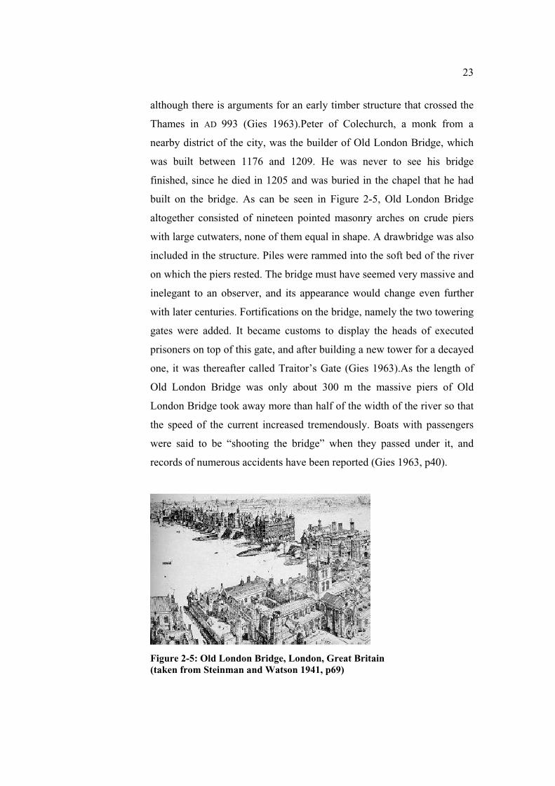
2.3.4 Construction and History of Old London Bridge

Probably the most colorful and vivid history, unsurpassed by any

other, is related to a bridge located in a city that gained an enormous

growth in the medieval times (Gies 1963, p47). London had been founded

by the Romans, who called it Londinium. Little is known about the

centuries after the Romans had left and about former bridges in London,

23

although there is arguments for an early timber structure that crossed the

Thames in AD 993 (Gies 1963).Peter of Colechurch, a monk from a

nearby district of the city, was the builder of Old London Bridge, which

was built between 1176 and 1209. He was never to see his bridge

finished, since he died in 1205 and was buried in the chapel that he had

built on the bridge. As can be seen in Figure 2-5, Old London Bridge

altogether consisted of nineteen pointed masonry arches on crude piers

with large cutwaters, none of them equal in shape. A drawbridge was also

included in the structure. Piles were rammed into the soft bed of the river

on which the piers rested. The bridge must have seemed very massive and

inelegant to an observer, and its appearance would change even further

with later centuries. Fortifications on the bridge, namely the two towering

gates were added. It became customs to display the heads of executed

prisoners on top of this gate, and after building a new tower for a decayed

one, it was thereafter called Traitor’s Gate (Gies 1963).As the length of

Old London Bridge was only about 300 m the massive piers of Old

London Bridge took away more than half of the width of the river so that

the speed of the current increased tremendously. Boats with passengers

were said to be “shooting the bridge” when they passed under it, and

records of numerous accidents have been reported (Gies 1963, p40).

Figure 2-5: Old London Bridge, London, Great Britain (taken from Steinman and Watson 1941, p69)

24

Located in the heart of London, Old London Bridge served the city for

more than six hundredyears, and for most of this time, about five and a

half centuries, it remained the only solid passing of the Thames. In 1740

finally, Westminster Bridge was built, and in 1831 building a new bridge

at the old location was begun.

Over all this long time Old London Bridge continuously changed

its appearance. Apart from the chapel already mentioned, more buildings

were added on top of the superstructure. Except for a few openings where

the river could actually be seen from the roadway, the bridge in its later

days carried literally dozens of houses. These were crammed at both sides

of the roadway, leaving only relatively little space in the middle. Wooden

frames held the houses together over the roadway, and some reportedly

even had basements under the arch spans, leaving even less room for

boats to pass. Even wheels were erected under several spans to power

watermills.Merchandising flourished on the bridge and tolls were

collected for passing it. The ease of water supply and wastewater removal

at the bridge made it a favorite place for the trades of the Londoners, Gies

(1963) lines out.

Many anecdotes and legends are attached to Old London Bridge.

It even once happened that a complete house fell off the bridge into the

Thames. As Steinman and Watson (1941, p64) put it,the “life story of this

six-hundred-year-old bridge would fill many a good-sized volume and

would include exciting accounts of fire, tournaments, battles, fairs, royal

processions, dramas,songs, and dances.” A highly readable description of

these centuries full of history is given in a chapter by Gies (1963).

25

2.3.5 The Era of Concrete Bridges and Beyond

The following sections will introduce the wide range of modern

bridge structures and their development. The main focus is placed on

concrete structures. Historic developments and characteristics of certain

types of concrete bridges will be presented. Certain specialties in bridges

will not be discussed, e.g. moving bridges of all kinds (i.e. bascule

bridges, lift and swing bridges), and highway bridges, many of which are

made of prefabricated concrete beams. The specific problems of skewed

and curved bridges are also excluded from this section.

2.3.6 Concrete Characteristics

Concrete had already been commonly in use in Roman times, as

described in early this section.Simple mortars had already been used

much earlier. Strong and waterproof mortars as the Romans had used,

however, were only rediscovered around the late eighteenth century, as

Brown (1993) notes.Concrete is an artificial stone-like inhomogeneous

material that is produced by mixing specified amounts of cement, water,

and aggregates. The first two ingredients react chemically to a hard

matrix, which acts as a binder. Most of the volume of the concrete is

taken by aggregates, which is the fill material. In modern concrete design

mixtures special mineral additives or chemical admixtures are added to

influence certain properties of the concrete. Strength can be increased

26

through use of special types of cement and a low water-cement ratio;

workability can be improved with retarders and superplasticizers; and

durability depends on the volume of air enclosed within the concrete.

Proportions and chemistry of the ingredients as well as the manner of

placement and curing determine the final concrete properties.Concrete is

the universal construction material of modern times due to several

advantages. It is formable into virtually any shape with formwork, its

ingredients are relatively cheap and can be found ubiquitously, it has a

high compressive strength and, provided good quality of workmanship, is

very durable at little maintenance cost.

Reinforced concrete is a composite material that is composed of

concrete and steel members that are embedded and bonded to it. These

steel bars or mats fulfill the purpose of enhancing the resistance of a

reinforced concrete member to tensile stresses, as concrete alone is strong

in compression but has less resistance to tension that is applied. The

amount and location of the reinforcement needed for a certain structure is

determined during its design. In sound concrete the steel reinforcement is

protected by the natural alkalinity of the concrete that creates a passifying

layer on the steel surface.

2.3.6.1 Early Concrete Structures

Several names are linked with the beginnings of reinforced

concrete. A comprehensive historical review of the developments that led

to application of reinforced concrete in the construction industry is given

by Menn (1990). In 1756 John Smeaton came up with a way of cement

production and in 1824 the mason Joseph Aspdin invented Portland

cement in England.Thaddeus Hyatt (1816 - 1901) examined behavior of

concrete beams as early as 1850 in the U.S.

27

Some years later, in 1867, French engineer Joseph Monier

received a patent on flowerpots whose concrete was reinforced with a

steel mesh. Monier also became first in building a bridge of reinforced

concrete in 1875 (Menn 1990). In the years to come, the first scientific

approaches to the behavior and analysis of reinforced concrete were taken

and opened the way to more and more advanced structures. French

engineer François Hennebique (1842 - 1931) researched T-shaped beams

and received patents on these around 1892, after which a larger number of

bridges was built in European countries in the following years. While

construction of reinforced concrete bridges spread across Europe, the first

national codes for reinforced concrete appeared.According to Menn

(1990), prior to the 1930s steel bridges still dominated the U.S. landscape

since they were cheaper and allowed rapid erection. In later years

reinforced concrete bridges became more common in the New World.

2.3.6.2 Concrete Arch Bridges

Robert Maillart (1872 - 1940) was exploring the structural

possibilities of the new construction material in an impressive diversity of

arch bridges in Switzerland. Located predominantly in mountainous

terrain the more than 40 bridges he designed were ingenious in their

slenderness, variability of shapes and beauty. It can be said that in his

structures all possibilities of concrete,including superior compressive

strength and formability were used to their full extent. One of his more

known structures is the daring shallow arch of the Salginatobel Bridge

that spans 90 m. In this bridge the superstructure was dissolved to a

slender arch that carried the deck with transverse wall panels. Melaragno

28

(1998, p19) in this context uses the term “structural art” to capture the

spirit of this unique family of concrete structures.

2.3.6.3 Prestressed Concrete Bridges

As early as 1888 a German engineer had examined prestressed

concrete members (Menn 1990).Yet it was Eugène Freyssinet (1879 -

1962), a graduate of the École des Ponts et Chaussées, who is considered

the father of prestressed concrete bridges. His most known bridge is the

Plougastel Bridge that was built between 1925 and 1930 in France. A

construction stage of this bridge is shown in Figure 2-28.

Figure 2-6: The Plougastel Bridge under Construction (taken fromBrown 1993, p122)

Three 186-m long arches of still normal reinforced concrete with a

box girder cross-section support a two level truss deck for road traffic and

railway. For this bridge Freyssinet employed large timber falsework that

was brought into place by pontoons and reused for all three arch spans.

Brown (1993) stresses the importance of this bridge with respect to

prestressing, since it was the Plougastel Bridge where Freyssinet became

aware of the phenomenon of concrete creep,which needs to be considered

29

in prestressed construction. Freyssinet implemented jacking the concrete

bridge spans apart prior to closure of the midspan gap to account for

creep. Between 1941 and 1949 a famous family of six prestressed

concrete bridges were built after Freyssinet’s design at the River Marne in

France, five of them with similar spans of 74 m (Menn1990). These

bridges were shallow frames with vertically prestressed thin girder webs

(Brown1993). Segments for these bridges were delivered by barges and

lifted into place in larger sets.Freyssinet came up with concepts for “both

pre-tensioned and post-tensioned concrete” (Menn 1990, p30) and thus

initiated the rapid development of prestressed concrete bridges.

2.4 Concrete Bridges after the Second World War

After the Second World War the European transportation

infrastructure needed to be rebuilt and extended. Steel box girders could

now be put together by welding instead of riveting. Some of the first of

these bridges were built at the Rhine by German engineer Fritz Leonhardt

(born 1909), who also designed a large number of concrete structures.

Box girders, which had been used for the arches of the Plougastel Bridge,

were more and more introduced in steel and concrete bridge construction

as better understanding of the properties and the inherent advantages of

closed hollow cross-sections grew. Prestressed concrete bridges were

built in large numbers. In Germany,Franz Dischinger (1887 - 1953) built

prestressed concrete bridges with a system different fromFreyssinet’s; he

used unbonded tendons that did not reach widespread application until

much later due to problems with loss of prestressing force (Menn 1990).

Subsequent development of different prestressing systems was therefore

based on the original Freyssinet system. Cast-in-place cantilever bridges

30

have been built for almost half a century. Ulrich Finsterwalder, student of

Dischinger, took the first step in erection with the balanced cantilevering

method when he built the 62-m long span of the Lahn Bridge at

Balduinstein in Germany between 1950 and 1951 (Fletcher 1984.

Prestressing of concrete bridges reduced deflections, prevented

cracking, and allowed higher loads to be carried by the bridges (Menn

1990). Freyssinet’s system of implementing full prestressing was not very

economical, though. Therefore, partial prestressing became prevalent as it

was introduced into the design codes. Partial prestressing permitted

limited tensile stressesin concrete and made use of mild reinforcement to

alleviate the cracking of the concrete because of these stresses.

Precast segmental construction emerged in the early 1960s, as

Menn (1990) also reports. In the following decades, solutions for the

problem of segments joints were developed, including match-casting of

the segments at the precasting yard, implementation of shear keys, and

use of epoxy agents that sealed and glued the joint faces together. In the

decades since the first prestressed concrete bridges were built many

technological achievements have been made. Research allowed better

understanding of the internal flow of forces in concrete and in the

embedded steel and helped improving material properties of these

construction materials.

2.4.1 Cable-Stayed Bridges

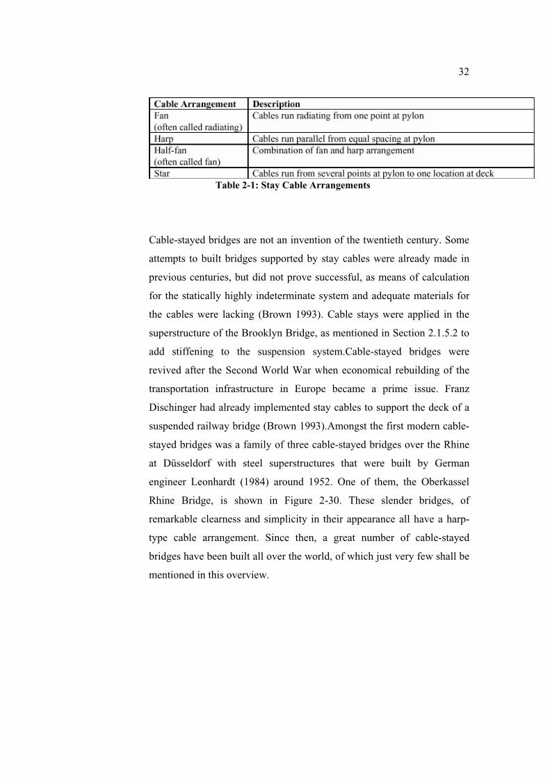
Cable-stayed bridges can appear in many different ways. The

bridge pylons and the bridge superstructure can be made either of

concrete or steel, or be a composite of concrete and steel members.

Pylons can be shaped in a great number of ways, including A, H, X, and

31

inverted V and Y-shapes, or combinations and variations of these. In a

cable-stayed bridge inclined straight stay cables that are attached to

pylons above the deck carry the bridge deck. A multitude of arrangements

for pylons and cable layout exists.

Furthermore, the bridge can be designed with one central or two

lateral planes of stay cables that can even be inclined toward each other.

Cable-stayed bridges can have several different arrangements for the stay

cables, as explained in Table 2-1. The respective arrangements are shown

in Figure 2-29. Cable arrangements do not necessarily have to be exactly

symmetric about the tower. Variations and combinations between these

types are possible. Cables can be anchored both on the deck and at the

pylon or can run continuously over a saddle at the top of the pylon the

anchorages for the stay cables are critical structural details that have to be

resistant to corrosion and fatigue.

Figure 2-7: Stay Cable Arrangements

32

Table 2-1: Stay Cable Arrangements

Cable-stayed bridges are not an invention of the twentieth century. Some

attempts to built bridges supported by stay cables were already made in

previous centuries, but did not prove successful, as means of calculation

for the statically highly indeterminate system and adequate materials for

the cables were lacking (Brown 1993). Cable stays were applied in the

superstructure of the Brooklyn Bridge, as mentioned in Section 2.1.5.2 to

add stiffening to the suspension system.Cable-stayed bridges were

revived after the Second World War when economical rebuilding of the

transportation infrastructure in Europe became a prime issue. Franz

Dischinger had already implemented stay cables to support the deck of a

suspended railway bridge (Brown 1993).Amongst the first modern cable-

stayed bridges was a family of three cable-stayed bridges over the Rhine

at Düsseldorf with steel superstructures that were built by German

engineer Leonhardt (1984) around 1952. One of them, the Oberkassel

Rhine Bridge, is shown in Figure 2-30. These slender bridges, of

remarkable clearness and simplicity in their appearance all have a harp-

type cable arrangement. Since then, a great number of cable-stayed

bridges have been built all over the world, of which just very few shall be

mentioned in this overview.

33

Figure 2-8: The Oberkassel Rhine Bridge, Düsseldorf, Germany (taken from Leonhardt 1984, p260)

The first concrete cable-stayed bridge was the Lake Maracaibo

Bridge in Venezuela, which was built between 1958 and 1962.

The designer Riccardo Morandi came up with a major concrete

structure with five main spans of 235 m length (Brown 1993). He

designed uniquely shaped pier tables that had a massive complex

X-shaped substructure, which carried A-shaped towers above the

deck level. The central concrete spans were comparatively

massive to achieve stiffness and were suspended with one group

of stay cables on each side of the towers. A view of the structure

with its characteristic approaches is shown in Figure 2-31.

Figure 2-9: The Lake Maracaibo Bridge, Venezuela (taken from Leonhardt 1984, p271)

34

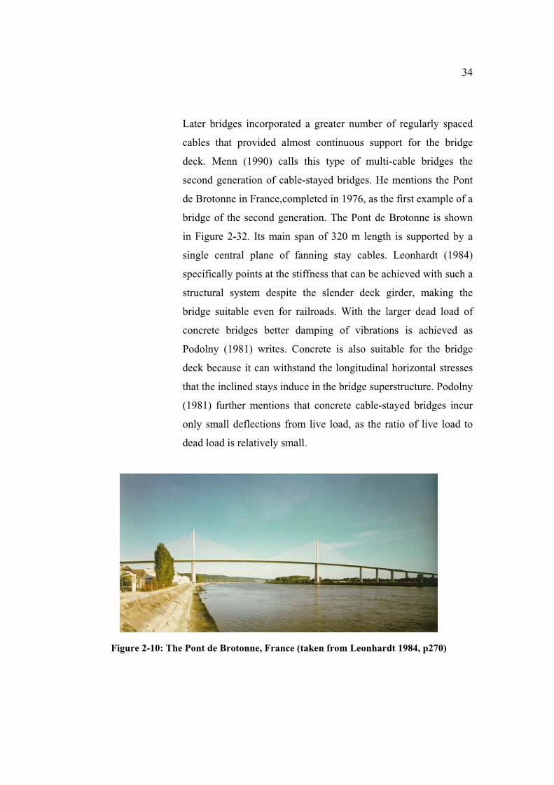
Later bridges incorporated a greater number of regularly spaced

cables that provided almost continuous support for the bridge

deck. Menn (1990) calls this type of multi-cable bridges the

second generation of cable-stayed bridges. He mentions the Pont

de Brotonne in France,completed in 1976, as the first example of a

bridge of the second generation. The Pont de Brotonne is shown

in Figure 2-32. Its main span of 320 m length is supported by a

single central plane of fanning stay cables. Leonhardt (1984)

specifically points at the stiffness that can be achieved with such a

structural system despite the slender deck girder, making the

bridge suitable even for railroads. With the larger dead load of

concrete bridges better damping of vibrations is achieved as

Podolny (1981) writes. Concrete is also suitable for the bridge

deck because it can withstand the longitudinal horizontal stresses

that the inclined stays induce in the bridge superstructure. Podolny

(1981) further mentions that concrete cable-stayed bridges incur

only small deflections from live load, as the ratio of live load to

dead load is relatively small.

Figure 2-10: The Pont de Brotonne, France (taken from Leonhardt 1984, p270)

35

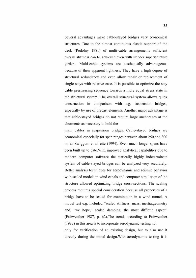
Several advantages make cable-stayed bridges very economical

structures. Due to the almost continuous elastic support of the

deck (Podolny 1981) of multi-cable arrangements sufficient

overall stiffness can be achieved even with slender superstructure

girders. Multi-cable systems are aesthetically advantageous

because of their apparent lightness. They have a high degree of

structural redundancy and even allow repair or replacement of

single stays with relative ease. It is possible to optimize the stay

cable prestressing sequence towards a more equal stress state in

the structural system. The overall structural system allows quick

construction in comparison with e.g. suspension bridges,

especially by use of precast elements. Another major advantage is

that cable-stayed bridges do not require large anchorages at the

abutments as necessary to hold the

main cables in suspension bridges. Cable-stayed bridges are

economical especially for span ranges between about 250 and 300

m, as Swiggum et al. cite (1994). Even much longer spans have

been built up to date.With improved analytical capabilities due to

modern computer software the statically highly indeterminate

system of cable-stayed bridges can be analyzed very accurately.

Better analysis techniques for aerodynamic and seismic behavior

with scaled models in wind canals and computer simulation of the

structure allowed optimizing bridge cross-sections. The scaling

process requires special consideration because all properties of a

bridge have to be scaled for examination in a wind tunnel. A

model test e.g. included “scaled stiffness, mass, inertia,geometry

and, “we hope,” scaled damping, the most difficult aspect”

(Fairweather 1987, p. 62).The trend, according to Fairweather

(1987) in this area is to incorporate aerodynamic testing not

only for verification of an existing design, but to also use it

directly during the initial design.With aerodynamic testing it is

36

also possible to evaluate the effects of innovative details for both

aerodynamic and seismic resistance. These details can be mass

dampers or tuned damping systems at bearings, joints, and cable

anchorages, installation of interconnecting ties between the stay

cables, and special shaping and texturing of the cables sheathing

to prevent vibrations from wind and rain.Cable-stayed bridges are

ideally erected with the cantilevering method. The stay cables

hence serve to support growing cantilever arms from above and

will also be the permanent supporting system for the bridge

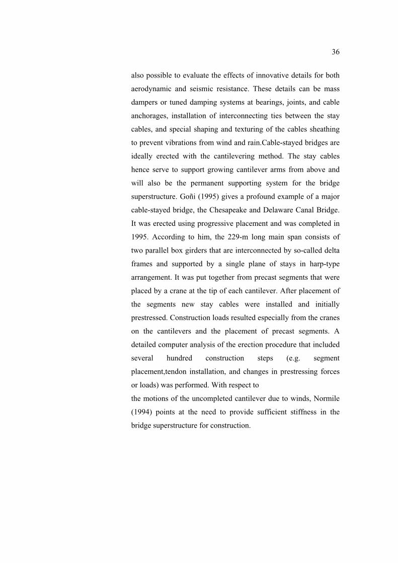
superstructure. Goñi (1995) gives a profound example of a major

cable-stayed bridge, the Chesapeake and Delaware Canal Bridge.

It was erected using progressive placement and was completed in

1995. According to him, the 229-m long main span consists of

two parallel box girders that are interconnected by so-called delta

frames and supported by a single plane of stays in harp-type

arrangement. It was put together from precast segments that were

placed by a crane at the tip of each cantilever. After placement of

the segments new stay cables were installed and initially

prestressed. Construction loads resulted especially from the cranes

on the cantilevers and the placement of precast segments. A

detailed computer analysis of the erection procedure that included

several hundred construction steps (e.g. segment

placement,tendon installation, and changes in prestressing forces

or loads) was performed. With respect to

the motions of the uncompleted cantilever due to winds, Normile

(1994) points at the need to provide sufficient stiffness in the

bridge superstructure for construction.

37

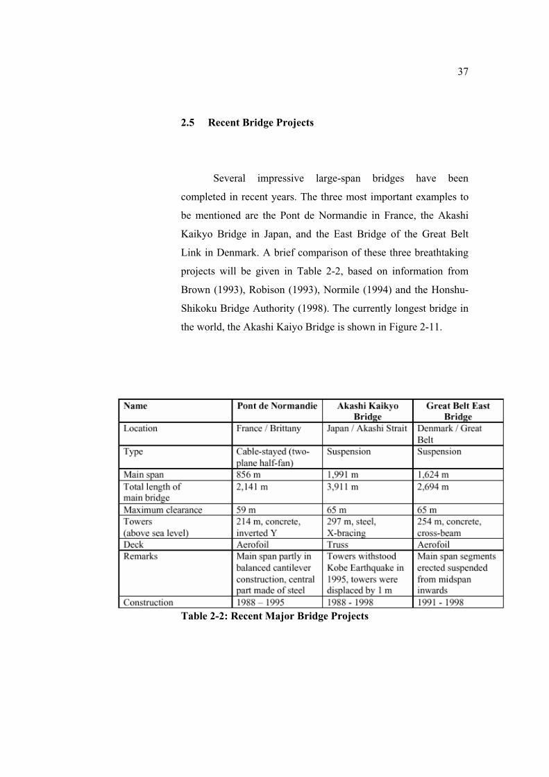
2.5 Recent Bridge Projects

Several impressive large-span bridges have been

completed in recent years. The three most important examples to

be mentioned are the Pont de Normandie in France, the Akashi

Kaikyo Bridge in Japan, and the East Bridge of the Great Belt

Link in Denmark. A brief comparison of these three breathtaking

projects will be given in Table 2-2, based on information from

Brown (1993), Robison (1993), Normile (1994) and the Honshu-

Shikoku Bridge Authority (1998). The currently longest bridge in

the world, the Akashi Kaiyo Bridge is shown in Figure 2-11.

Table 2-2: Recent Major Bridge Projects

38

Figure 2-11: The Akashi Kaikyo Bridge, Japan (taken from Honshu-ShikokuBridge Authority 1998, p1)

2.6 Contributions of Modern Concrete Bridge Construction

The introduction of concrete into bridge construction

opened almost unlimited new possibilities for the profession. The

several advantages of concrete, such as free formability, strength,

and durability came to full use in bridge construction and

contributed much to successful use of concrete in other branches.

Through use of steel reinforcement to bear the tensile stresses in

the members a composite material was created that combined

positive characteristics of both concrete and steel and could be

strengthened exactly as needed for a certain structure.Prestressing

39

concrete by means of tendons that are installed in the bridge

superstructure made extremely long, yet economical spans

possible. European engineers, such as Freyssinet carried the

prestressing concepts further. Other engineers, e.g. Maillart

explored structural possibilities along with artful shaping of

concrete bridges.Along with growing understanding of the

properties of the new material went the development of a variety

of construction methods that will be presented in Section 4.2.

Choice of either cast-in- place construction, precast construction,

or a combination of both methods made it possible to adapt

construction procedures exactly to the requirements of the specific

site and the project conditions.

The concept of box girder superstructures had already

been used in bridges as e.g. the Britannia Bridge. Since the end of

the Second World War the versatile box girders have become a

widely used type of superstructure cross-section.With cable-

stayed bridges a relatively new type of bridge rapidly developed

in the second half of the twentieth century. Economical and

elegant long-span cable-stayed bridges were subsequently built

that were only surpassed in length by a handful of the longest of

all bridges, which are suspension bridges.

CHAPTER III

THEORITICAL BACKGROUND

3.1 Choice of Abutment

Current practice is to make decks integral with the abutments. The

objective is to avoid the use of joints over abutments and piers. Expansion

joints are prone to leak and allow the ingress of de-icing salts into the bridge

deck and substructure. In general all bridges are made continuous over

intermediate supports and decks under 60 metres long with skews not

exceeding 30° are m ade integral with their abutments.

Figure 3.1: Open Side Span

41

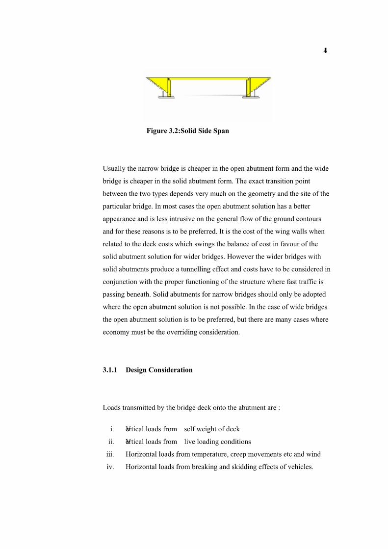
Figure 3.2:Solid Side Span

Usually the narrow bridge is cheaper in the open abutment form and the wide

bridge is cheaper in the solid abutment form. The exact transition point

between the two types depends very much on the geometry and the site of the

particular bridge. In most cases the open abutment solution has a better

appearance and is less intrusive on the general flow of the ground contours

and for these reasons is to be preferred. It is the cost of the wing walls when

related to the deck costs which swings the balance of cost in favour of the

solid abutment solution for wider bridges. However the wider bridges with

solid abutments produce a tunnelling effect and costs have to be considered in

conjunction with the proper functioning of the structure where fast traffic is

passing beneath. Solid abutments for narrow bridges should only be adopted

where the open abutment solution is not possible. In the case of wide bridges

the open abutment solution is to be preferred, but there are many cases where

economy must be the overriding consideration.

3.1.1 Design Consideration

Loads transmitted by the bridge deck onto the abutment are :

i. Vertical loads from self weight of deck

ii. Vertical loads from live loading conditions

iii. Horizontal loads from temperature, creep movements etc and wind

iv. Horizontal loads from breaking and skidding effects of vehicles.

42

These loads are carried by the bearings which are seated on the

abutment bearing platform. The horizontal loads may be reduced by

depending on the coefficient of friction of the bearings at the movement joint

in the structure.

However, the full breaking effect is to be taken, in either direction, on top of

the abutment at carriageway level.

In addition to the structure loads, horizontal pressures exerted by the fill

material against the abutment walls is to be considered. Also a vertical

loading from the weight of the fill acts on the footing.

Vehicle loads at the rear of the abutments are considered by applying a

surcharge load on the rear of the wall.

For certain short single span structures it is possible to use the bridge deck to

prop the two abutments apart. This entails the abutment wall being designed

as a propped cantilever.

3.2 Choice Of Bearing

Bridge bearings are devices for transferring loads and movements

from the deck to the substructure and foundations.

In highway bridge bearings movements are accommodated by the basic

mechanisms of internal deformation (elastomeric), sliding (PTFE), or rolling.

A large variety of bearings have evolved using various combinations of these

mechanisms.

43

Figure 3.3: Elastomeric Bearing Figure 3.4:Plane Sliding Bearing

Figure 3.5 : Multiple Roller Bearing

The functions of each bearing type are :

a) Elastomeric

The elastomeric bearing allows the deck to translate and rotate, but also resists loads

in the longitudinal, transverse and vertical directions. Loads are developed, and

movement is accommodated by distorting the elastomeric pad.

b) Plane Sliding

Sliding bearings usually consist of a low friction polymer, polytetrafluoroethylene

(PTFE), sliding against a metal plate. This bearing does not accommodate rotational

movement in the longitudinal or transverse directions and only resists loads in the vertical

direction. Longitudinal or transverse loads can be accommodated by providing

mechanical keys. The keys resist movement, and loads in a direction perpendicular to the

keyway.

44

b) Roller

Large longitudinal movements can be accommodated by these bearings, but vertical

loads only can generally be resisted.

The designer has to assess the maximum and minimum loads that the deck will exert

on the bearing together with the anticipated movements (translation and rotation).

Bearing manufacturers will supply a suitable bearing to meet

Figure 3.6 : Typical Bearing Layout

Bearings are arranged to allow the deck to expand and contract, but retain the

deck in its correct position on the substructure. A 'Fixed' Bearing does not allow

translational movement. 'Sliding Guid ed' Bearings are provided to restrain the deck in

all translational directions except in a radial direction from the fixed bearing. This

allows the deck to expand and contract freely. 'Sliding' Bearings are provided for

vertical support to the deck only.

3.2.1 Preliminary Design

In selecting the correct bridge type it is necessary to find a structure that will

perform its required function and present an acceptable appearance at the least cost.

Decisions taken at preliminary design stage will influence the extent to which the

actual structure approximates to the ideal, but so will decisions taken at detailed

design stage. Consideration of each of the ideal characteristics in turn will give some

indication of the importance of preliminary bridge design.

45

a. Safety.

The ideal structure must not collapse in use. It must be capable of

carrying the loading required of it with the appropriate factor of

safety. This is more significant at detailed design stage as generally

any sort of preliminary design can be made safe.

b. Serviceability.

The ideal structure must not suffer from local deterioration/failure,

from excessive deflection or vibration, and it must not interfere with

sight lines on roads above or below it. Detailed design cannot correct

faults induced by bad preliminary design.

c. Economy.

The structure must make minimal demands on labour and capital; it

must cost as little as possible to build and maintain. At preliminary

design stage it means choosing the right types of material for the

major elements of the structure, and arranging these in the right form.

d. Appearance.

The structure must be pleasing to look at. Decisions about form and

materials are made at preliminary design stage; the sizes of individual

members are finalised at detailed design stage. The preliminary

design usually settles the appearance of the bridge.

3.2.2 Constraint

The construction depth available should be evaluated. The economic

implications of raising or lowering any approach embankments should then be

considered. By lowering the embankments the cost of the earthworks may be

reduced, but the resulting reduction in the construction depth may cause the deck to

be more expensive. If the bridge is to cross a road that is on a curve, then the width of

the opening may have to be increased to provide an adequate site line for vehicles on

46

the curved road.

It is important to determine the condition of the bridge site by carrying out a

comprehensive site investigation. BS 5930: Code of practice for Site Investigations

includes such topics as:

i. Soil survey

ii. Existing services (Gas, Electricity, Water, etc)

iii. Rivers and streams (liability to flood)

iv. Existing property and rights of way

v. Access to site for construction traffic

3.3 Selection of Bridge Type

Span Deck Type

Up to 20m

Insitu reinforced concrete.

Insitu prestressed post-tensioned concrete.

Prestressed pre-tensioned inverted T beams with insitu fill.

16m to 30m

Insitu reinforced concrete voided slab.

Insitu prestressed post-tensioned concrete voided slab.

Prestressed pre-tensioned M and I beams with insitu slab.

Prestressed pre-tensioned box beams with insitu topping.

Prestressed post-tensioned beams with insitu slab.

Steel beams with insitu slab.

30m to 40m

Prestressed pre-tensioned SY beams with insitu slab.

Prestressed pre-tensioned box beams with insitu topping.

Prestressed post-tensioned beams with insitu slab.

Steel beams with insitu slab.

30m to 250m Box girder bridges - As the span increases the construction tends to go from 'all

47

concrete' to 'steel box / concrete deck' to 'all steel'.

Truss bridges - for spans up to 50m they are generally less economic than plate

girders.

150m to 350m Cable stayed bridges.

350m > Suspension bridges.

Table 3.1 : selection of bridge type for various span length

3.3.1 Preliminary Design Consideration

1. A span to depth ratio of 20 will give a starting point for estimating

construction depths.

2. Continuity over supports

i. Reduces number of expansion joints.

ii. Reduces maximum bending moments and hence construction

depth or the material used.

3. Increases sensitivity to differential settlement. Factory made units

i. Reduces the need for soffit shuttering or scaffolding; useful

when headroom is restricted or access is difficult.

ii. Reduces site work which is weather dependent.

iii. Dependent on delivery dates by specialist manufactures.

iv. Specials tend to be expensive.

v. Special permission needed to transport units of more than

29m long on the highway

4. Length of structure

i. The shortest structure is not always the cheapest. By

increasing the length of the structure the embankment,

48

retaining wall and abutment costs may be reduced, but the

deck costs will increase.

5. Substructure

i. The structure should be considered as a whole, including

appraisal of piers, abutments and foundations. Alternative

designs for piled foundations should be investigated; piling

can increase the cost of a structure by up to 20%.

The preliminary design process will produce several apparently viable schemes.

The procedure from this point is to:

i. Estimate the major quantities.

ii. Apply unit price rates - they need not be up to date but should reflect any differential

variations.

iii. Obtain prices for the schemes.

3.3.2 Design Standard for preliminary design

The final selection will be based on cost and aesthetics. This method of

costing assumes that the scheme with the minimum volume will be the cheapest, and

will be true if the structure is not particularly unusual

i. BS 5400: Part 1: General Statement

ii. BS 5400: Part 2: Specification for Loads

iii. BS 5930: Code of Practice for Site Investigations

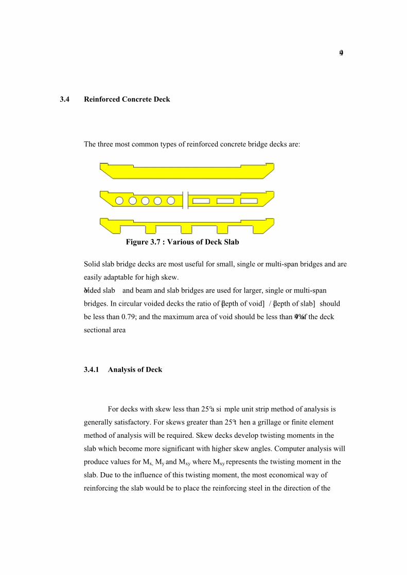
49

3.4 Reinforced Concrete Deck

The three most common types of reinforced concrete bridge decks are:

Figure 3.7 : Various of Deck Slab

Solid slab bridge decks are most useful for small, single or multi-span bridges and are

easily adaptable for high skew.

Voided slab and beam and slab bridges are used for larger, single or multi-span

bridges. In circular voided decks the ratio of [depth of void] / [depth of slab] should

be less than 0.79; and the maximum area of void should be less than 49% of the deck

sectional area

3.4.1 Analysis of Deck

For decks with skew less than 25° a si mple unit strip method of analysis is

generally satisfactory. For skews greater than 25° t hen a grillage or finite element

method of analysis will be required. Skew decks develop twisting moments in the

slab which become more significant with higher skew angles. Computer analysis will

produce values for Mx, My and Mxy where Mxy represents the twisting moment in the

slab. Due to the influence of this twisting moment, the most economical way of

reinforcing the slab would be to place the reinforcing steel in the direction of the

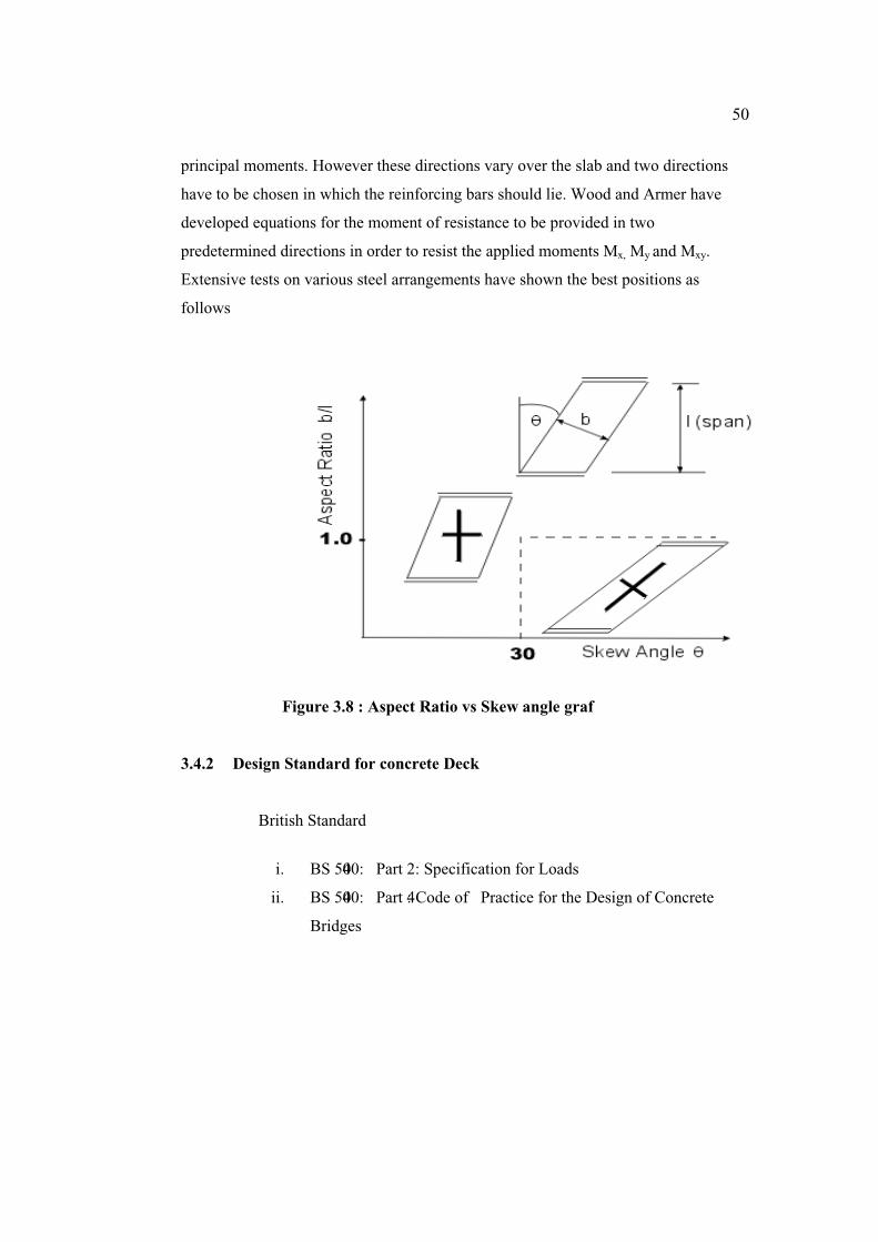
50

principal moments. However these directions vary over the slab and two directions

have to be chosen in which the reinforcing bars should lie. Wood and Armer have

developed equations for the moment of resistance to be provided in two

predetermined directions in order to resist the applied moments Mx, My and Mxy.

Extensive tests on various steel arrangements have shown the best positions as

follows

Figure 3.8 : Aspect Ratio vs Skew angle graf

3.4.2 Design Standard for concrete Deck

British Standard

i. BS 5400: Part 2: Specification for Loads

ii. BS 5400: Part 4: Code of Practice for the Design of Concrete

Bridges

51

3.4.3 Prestressed Concrete Deck

There are two types of deck using prestressed concrete :

i. Pre-tensioned beams with insitu concrete.

ii. Post-tensioned concrete.

The term pre-tensioning is used to describe a method of prestressing in which

the tendons are tensioned before the concrete is placed, and the prestress is

transferred to the concrete when a suitable cube strength is reached.

Post-tensioning is a method of prestressing in which the tendon is tensioned

after the concrete has reached a suitable strength. The tendons are anchored

against the hardened concrete immediately after prestressing.

There are three concepts involved in the design of prestressed concrete :

i. Prestressing transforms concrete into an elastic material.

By applying this concept concrete may be regarded as an elastic

material, and may be treated as such for design at normal working

loads. From this concept the criterion of no tensile stresses in the

concrete was evolved.

In an economically designed simply supported beam, at the

critical section, the bottom fibre stress under dead load and

prestress should ideally be the maximum allowable stress; and

under dead load, live load and prestress the stress should be the

minimum allowable stress.

Therefore under dead load and prestress, as the dead load moment

reduces towards the support, then the prestress moment will have

to reduce accordingly to avoid exceeding the permissible stresses.

In post-tensioned structures this may be achieved by curving the

tendons, or in pre-tensioned structures some of the prestressing

strands may be deflected or de-bonded near the support.

52

ii. Prestressed concrete is to be considered as a combination of steel

and concrete with the steel taking tension and concrete

compression so that the two materials form a resisting couple

against the external moment. (Analogous to reinforced concrete

concepts).

This concept is utilized to determine the ultimate strength of

prestressed beams.

iii. Prestressing is used to achieve load balancing.

It is possible to arrange the tendons to produce an upward load

which balances the downward load due to say, dead load, in

which case the concrete would be in uniform compression.

3.4.4 Pre-Tension Bridge Deck

Pre-tensioned bridge decks are composed of prestressed beams, which

have been prestressed off site, together with insitu concrete forming a slab

and in some cases filling the voids between the beams.

T-Beam M-Beam Y-Beam

Figure 3.9 : Type of Girder

Types of beams in common use are inverted T-beams, M-beams and

Y beam s. Inverted T-beams are generally used for spans between 7 and 16

53

metres and the voids between the beams are filled with insitu concrete thus

forming a solid deck. M-Beams are used for spans between 14 an d 30 metres

and have a thin slab cast insitu spanning between the top flanges. The Y-

beam was introduced in 1990 to replace the M-beam. This lead to the

production of an SY-bea m which is used for spans between 32 and 40 m etres.

Post-tensioned bridge decks are generally composed of insitu concrete in

which ducts have been cast in the required positions..

T-Beam Voided Slab Box

Span < 35m 20m < Span < 35m Span > 30m

Figure 3.10 : Types of Beam-Slab

When the concrete has acquired sufficient strength, the tendons are

threaded through the ducts and tensioned by hydraulic jacks acting against

the ends of the member. The ends of the tendons are then anchored.

Tendons are then bonded to the concrete by injecting grout into the ducts

after the stressing has been completed.

It is possible to use pre-cast concrete units which are post-tensioned

together on site to form the bridge deck.

Generally it is more economical to use post-tensioned construction for

continuous structures rather than insitu reinforced concrete at spans

greater than 20 metres. For simply supported spans it may be economic to

use a post-tensioned deck at spans greater than 20 metres.

54

3.5 Composite Deck

Composite Construction in bridge decks usually refers to the

interaction between insitu reinforced concrete and structural steel.

Three main economic advantages of composite construction are :

i. For a given span and loading system a smaller depth of beam can be used

than for a concrete beam solution, which leads to economies in the approach

embankments.

ii. The cross-sectional area of the steel top flange can be reduced because the

concrete can be considered as part of it.

iii. Transverse stiffening for the top compression flange of the steel beam can

be reduced because the restraint against buckling is provided by the

concrete deck.

Figure 3.11: Typical Composite Deck

3.5.1 Construction Method

It is possible to influence the load carried by a composite deck section

in a number of ways during the erection of a bridge.

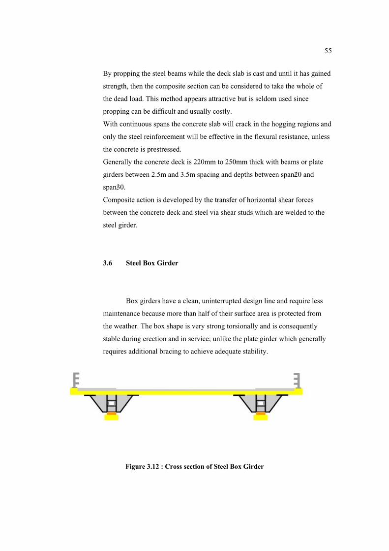
55

By propping the steel beams while the deck slab is cast and until it has gained

strength, then the composite section can be considered to take the whole of

the dead load. This method appears attractive but is seldom used since

propping can be difficult and usually costly.

With continuous spans the concrete slab will crack in the hogging regions and

only the steel reinforcement will be effective in the flexural resistance, unless

the concrete is prestressed.

Generally the concrete deck is 220mm to 250mm thick with beams or plate

girders between 2.5m and 3.5m spacing and depths between span/20 and

span/30.

Composite action is developed by the transfer of horizontal shear forces

between the concrete deck and steel via shear studs which are welded to the

steel girder.

3.6 Steel Box Girder

Box girders have a clean, uninterrupted design line and require less

maintenance because more than half of their surface area is protected from

the weather. The box shape is very strong torsionally and is consequently

stable during erection and in service; unlike the plate girder which generally

requires additional bracing to achieve adequate stability.

Figure 3.12 : Cross section of Steel Box Girder

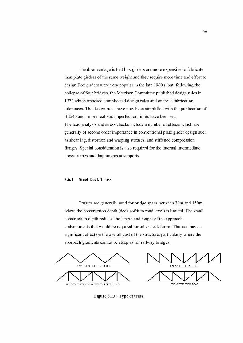
56

The disadvantage is that box girders are more expensive to fabricate

than plate girders of the same weight and they require more time and effort to

design.Box girders were very popular in the late 1960's, but, following the

collapse of four bridges, the Merrison Committee published design rules in

1972 which imposed complicated design rules and onerous fabrication

tolerances. The design rules have now been simplified with the publication of

BS5400 and more realistic imperfection limits have been set.

The load analysis and stress checks include a number of effects which are

generally of second order importance in conventional plate girder design such

as shear lag, distortion and warping stresses, and stiffened compression

flanges. Special consideration is also required for the internal intermediate

cross-frames and diaphragms at supports.

3.6.1 Steel Deck Truss

Trusses are generally used for bridge spans between 30m and 150m

where the construction depth (deck soffit to road level) is limited. The small

construction depth reduces the length and height of the approach

embankments that would be required for other deck forms. This can have a

significant effect on the overall cost of the structure, particularly where the

approach gradients cannot be steep as for railway bridges.

Figure 3.13 : Type of truss

57

High fabrication and maintenance costs has made the truss type deck less

popular in the UK; labour costs being relatively high compared to material

costs. Where material costs are relatively high then the truss is still an

economical solution. The form of construction also allows the bridge to be

fabricated in small sections off site which also makes transportation easier,

particularly in remote areas.

3.6.2 Choice of Truss

Figure 3.14 : Bridge Truss

The underslung truss is the most economical as the deck provides

support for the live load and also braces the compression chord. There is

however the problem of the headroom clearance required under the deck

which generally renders this truss only suitable for unnavigable rivers or over

flood planes.

Where underslung trusses are not possible, and the span is short, it

may be economical to use a half-through truss. Restraint to the compression

flange is achieved by U frame action.

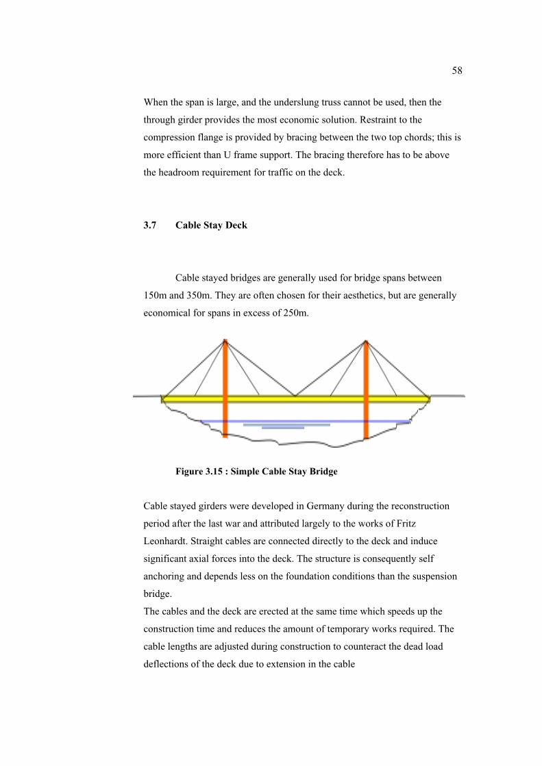
58

When the span is large, and the underslung truss cannot be used, then the

through girder provides the most economic solution. Restraint to the

compression flange is provided by bracing between the two top chords; this is

more efficient than U frame support. The bracing therefore has to be above

the headroom requirement for traffic on the deck.

3.7 Cable Stay Deck

Cable stayed bridges are generally used for bridge spans between

150m and 350m. They are often chosen for their aesthetics, but are generally

economical for spans in excess of 250m.

Figure 3.15 : Simple Cable Stay Bridge

Cable stayed girders were developed in Germany during the reconstruction

period after the last war and attributed largely to the works of Fritz

Leonhardt. Straight cables are connected directly to the deck and induce

significant axial forces into the deck. The structure is consequently self

anchoring and depends less on the foundation conditions than the suspension

bridge.

The cables and the deck are erected at the same time which speeds up the

construction time and reduces the amount of temporary works required. The

cable lengths are adjusted during construction to counteract the dead load

deflections of the deck due to extension in the cable

59

Decks are usually of orthortropic steel plate construc

slabs can be used for spans up to about 250m. Either box girders or plate

girders can be used in the deck, however if a single plane of cables is used

then it is essential to use the box girder construction to achieve torsional

stability.

tion however composite

3.8 Suspension Bridges

Suspension bridges are used for bridge spans in excess of 350m.

Figure 3.16 : Suspension Bridge

Plans have now been approved to build a 3300m span suspension bridge

ers.

The

The Design Manual for Roads and Bridges BD 52/93 defines a

Parapet

across the Strait of Messina.A number of early suspension bridges were

designed without the appreciation of wind effects. Large deflections were

developed in the flexible decks and wind loading created unstable

oscillations. The problem was largely solved by using inclined hang

The suspension bridge is essentially a catenary cable prestressed by dead

weight. The cables are guided over the support towers to ground anchors.

stiffened deck is supported mainly by vertical or inclined hangers.

as "A protective fence or wall at the edge of a bridge or similar

structure.

60

Figure 3.17 : Types of Parapet

Manufacturers have developed and tested parapets to meet the containment

standards specified in the codes. Much of the earlier testing work was

involved with achieving a parapet which would absorb the impact load and

not deflect the vehicle back into the line of adjacent traffic. The weight of

vehicle, speed of impact and angle of impact influence the behaviour of the

parapet. Consequently a level of containment has been adopted to minimise

the risk to traffic using the bridge (above and below the deck).

The Design Manual for Roads and Bridges BD 52/93 Specifies a Group

Designation for various containment levels as follows :

Parapet Group

DesignationApplication

Containment for which

designed

P1 Vehicle parapets for brid ges carrying motorways or

roads to motorway standards (excluding motorway

bridges over railways and high risk locations).

1.5t vehicle at 113 km/h

and 20° angl e of impact.

P2 Vehicle/pedestrian parape ts for bridges carrying all

purpose roads and for accommodation bridges

(excluding bridges over railways and high risk

locations).

1.5t vehicle at 113 km/h

and 80 km/h and 20°

angle of impact.

P4 Pedestrian parapets for use on footbridges and

bridges carrying bridleways (excluding bridges over

railways).

1.4 kN/m perpendicular

to the parapet.

61

Parapets for use over railways (excluding use on

bridges at high risk railway locations).

i. on bridges carrying motorways or roads to

motorways or roads to motorway standards As for P1

ii. on bridges carrying all purpose roads As for P1

P5

iii. on footbridges As for P4

P6 High Containment vehicle and vehicle/pedestrian

parapets at high risk locations (excluding

accommodation bridges).

30t vehicle at 64 km/h

and 20° angle of impact.

Table 3.2 : The Design Manual for Roads and Bridges BD 52/93 Specifies a Group Designation

The Group Designation in the table above have the equivalent level of

containment as defined in BS 6779 as follows :

i. P1 & P2 (113) : Normal level of containment.

ii. P2 (80) : Low level of containment.

iii. P5 (excluding Footbridges) : Normal level of containment.

iv. P6 : High level of containment.

v.

3.8.1 Design Consideration

Normal and low level of containment strength requirements for

parapet posts and rails are given in terms of the products of the plastic moduli

of their geometric sections and the minimum yield stress of the material used.

Consequently the parapet will deform to absorb the impact load. Higher loads

than the designed containment load will fail the member at impact. If the

parapet post fails then the rails will mobilise lengths of the parapet adjacent to

the failed section to retain the vehicle. Concrete parapets are ideal for high

containment parapets due to their significant mass.

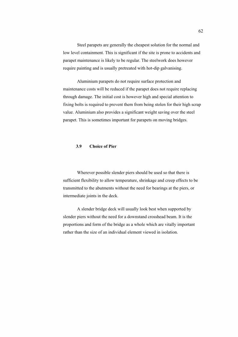
62

Steel parapets are generally the cheapest solution for the normal and

low level containment. This is significant if the site is prone to accidents and

parapet maintenance is likely to be regular. The steelwork does however

require painting and is usually pretreated with hot-dip galvanising.

Aluminium parapets do not require surface protection and

maintenance costs will be reduced if the parapet does not require replacing

through damage. The initial cost is however high and special attention to

fixing bolts is required to prevent them from being stolen for their high scrap

value. Aluminium also provides a significant weight saving over the steel

parapet. This is sometimes important for parapets on moving bridges.

3.9 Choice of Pier

Wherever possible slender piers should be used so that there is

sufficient flexibility to allow temperature, shrinkage and creep effects to be

transmitted to the abutments without the need for bearings at the piers, or

intermediate joints in the deck.

A slender bridge deck will usually look best when supported by

slender piers without the need for a downstand crosshead beam. It is the

proportions and form of the bridge as a whole which are vitally important

rather than the size of an individual element viewed in isolation.

63

Figure 3.18 : Different Pier Shape

3.9.1 Design Consideration

Loads transmitted by the bridge deck onto the pier are :

i. Vertical loads from self weight of deck

ii. Vertical loads from live loading conditions

iii. Horizontal loads from temperature, creep movements etc and

wind

iv. Rotations due to deflection of the bridge deck.

The overall configuration of the bridge will determine the

combination of loads and movements that have to be designed for. For

example if the pier has a bearing at its top, corresponding to a structural pin

joint, then the horizontal movements will impose moments at the base, their

magnitude will depend on the pier flexibility.

Sometimes special requirements are imposed by rail or river authorities if

piers are positioned within their jurisdiction. In the case of river authorities a

'cut water ' may be required to assist the river flow, or independent fenders to

protect the pier from impact from boats or floating debris. A similar

arrangement is often required by the rail authorities to prevent minor

derailments striking the pier. Whereas the pier has to be designed to resist

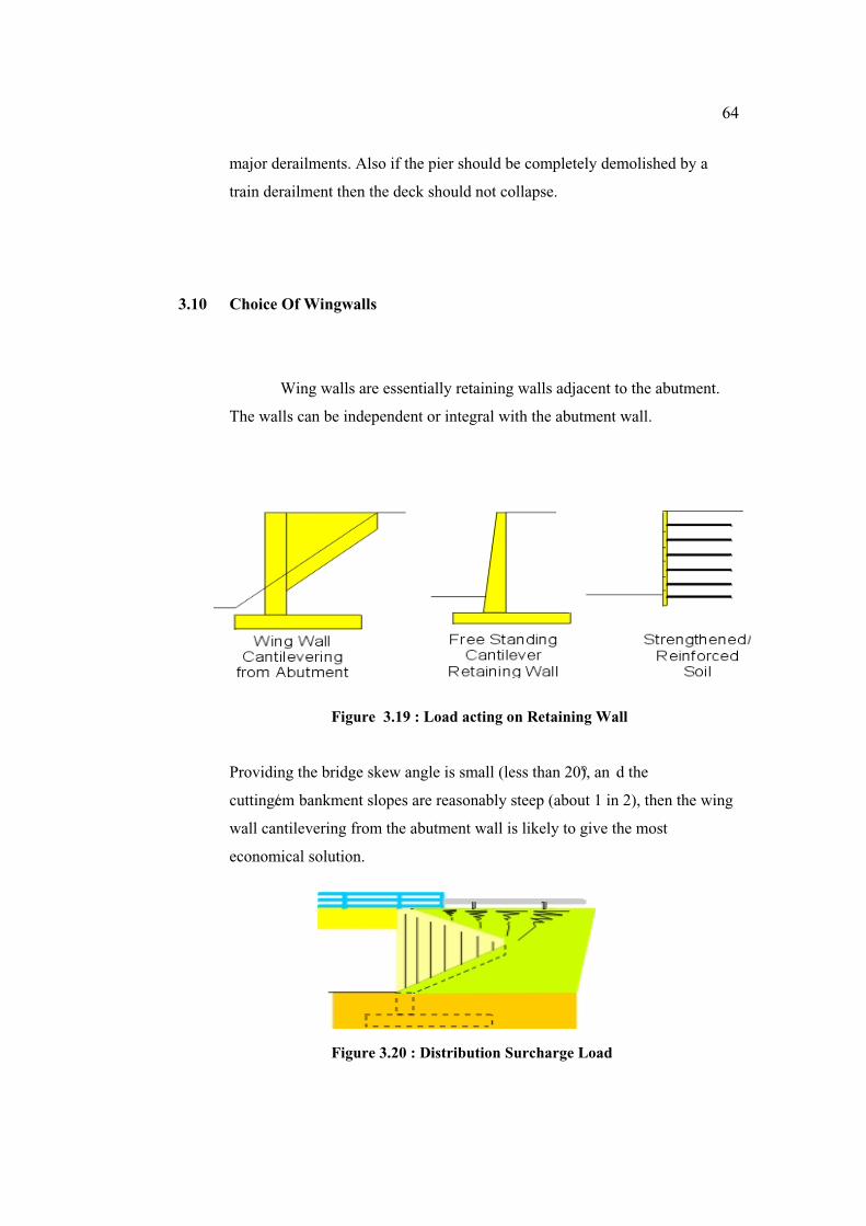
64

major derailments. Also if the pier should be completely demolished by a

train derailment then the deck should not collapse.

.10 Choice Of Wingwalls

Wing walls are essentially retaining walls adjacent to the abutment.

The wa

Figure 3.19 : Load acting on Retaining Wall

Providing the bridge skew angle is small (less than 20°), an d the

en the wing

3

lls can be independent or integral with the abutment wall.

cutting/em bankment slopes are reasonably steep (about 1 in 2), th

wall cantilevering from the abutment wall is likely to give the most

economical solution.

Figure 3.20 : Distribution Surcharge Load

65

Splayed wing walls provide even more of an economy in material costs but

the detailing and fixing of the steel reinforcement is more complicated than

3.10.1 Design Consideration

Loads effects to be considered on the rear of the wall are:

ii. Surcharge from live loading or compacting plant.

i ns.

T ta tive' earth

pressures (Ka); whilst the structural elements are designed to resist 'at rest'

earth pr

se

hen

the conventional wall.

i. Earth pressures from the backfill material.

ii. Hydraulic loads from saturated soil conditio

he s bility of the wall is generally designed to resist 'ac

essures (Ko). The concept is that 'at rest' pressures are developed

initially and the structural elements should be designed to accommodate the

loads without failure. The loads will however reduce to 'active' pressure w

the wall moves, either by rotating or sliding. Consequently the wall will

stabilise if it moves under 'at rest' pressures providing it is designed to resist

'active' earth pressures.

CHAPTER IV

METHODOLOGY

4.1 Introduction

This chapter discuss the ways on how to compare the different

usage of code of practices and the steps for each codes in getting a result

of design of structure members. In this case, we redesign an existing

bridge structure that available in our selecting bridge in Malaysia.This

bridge was designed using the usual code in Malaysia known as BS 5400.

In our research, we take this existing of structure and try redesign

by using another method or code of practice to compare a size and cost of

structure when using different code of practices. For this case, we select

AASHTO-SEISMIC design code as our comparison code. We have

defined for value of seismic or reading based on previous event that

occurred in our country.For peninsular Malaysia, a reading of seismic

value we assign as 0.075 g (75 gal). Meanwhile for Sabah and Sarawak,

we assign as 0.15 g (150 gal).We get these both values from Malaysia

Meteorological Services Department.

Section 4.2 will show the design flow chart for each codes that we

apply i.e. sequence of steps in design calculation of members.After that,

our result will be described in section 4.3 by analyzing the outcome from

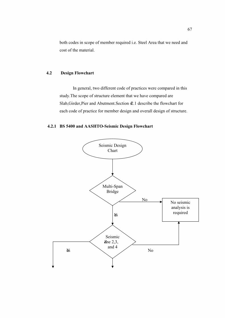
67

both codes in scope of member required i.e. Steel Area that we need and

cost of the material.

4.2 Design Flowchart

In general, two different code of practices were compared in this

study.The scope of structure element that we have compared are

Slab,Girder,Pier and Abutment.Section 4.2.1 describe the flowchart for

each code of practice for member design and overall design of structure.

4.2.1 BS 5400 and AASHTO-Seismic Design Flowchart

No

Yes

Yes No

No seismicanalysis is required

SeismicZone 2,3,

and 4

Multi-SpanBridge

Seismic Design Chart

68

Yes

No No

Yes Yes

Yes No Yes No

Yes No

CriticalBridge

Other Bridge

Regular

Zone m ethod2 MM3 MM4 TH

Zone m ethod2 MM 3 TH 4 TH

Regular

Zone m ethod 2 SM/UL3 MM

4 MM

Zone m ethod 2 MM3 MM

4 MM

Zone m ethod 2 SM/UL3 SM/UL

4 SM/UL

Zone m ethod 2 SM3 MM

4 MM

EssentialBridges

69

Select Modification Factor R

Design Components based on F/R

END

Design Detail : Connections between superstructure and substructure, and seat width

SM-Single Mode Spectral Method

UL-Uniform Load Method

MM-Multi mode Spectral Method

TH-Time History

Figure 4.1 : AASHTO–LRFD seismic design flowchart

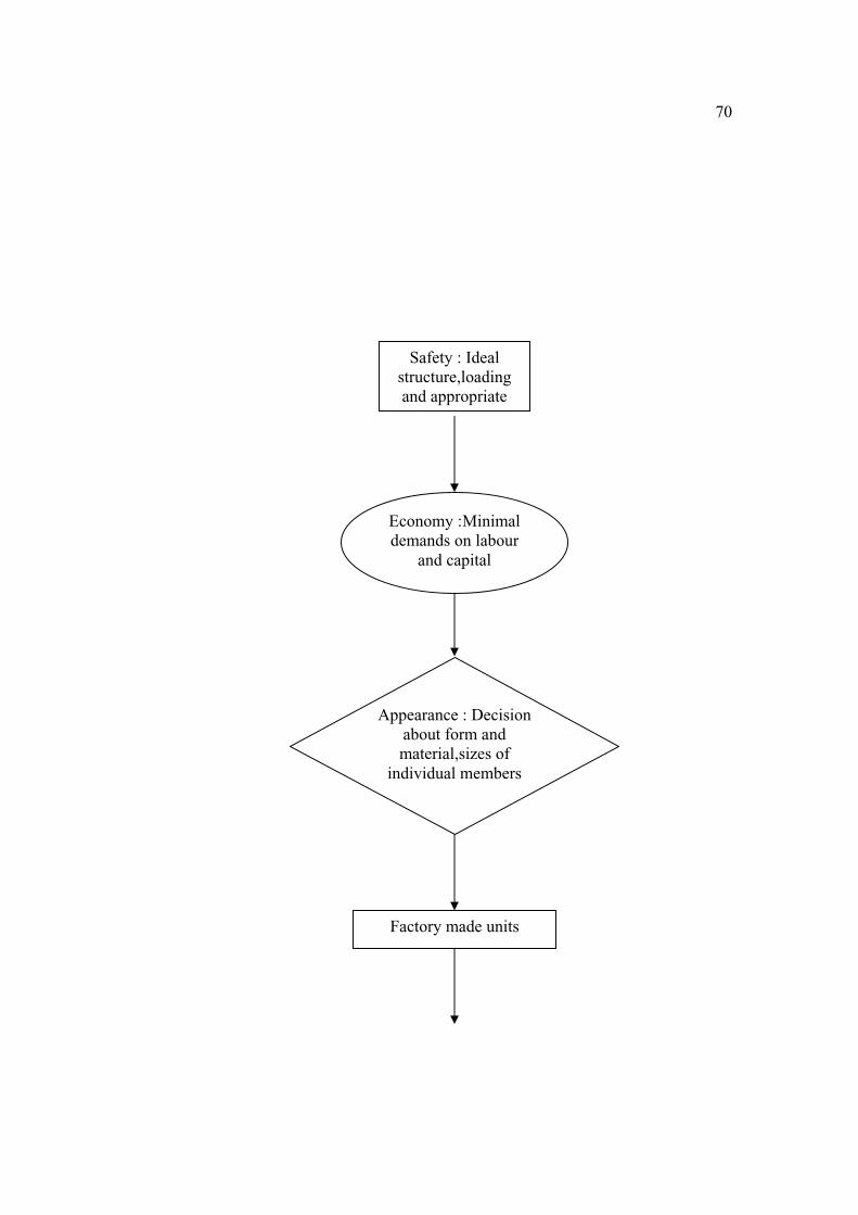
70

Safety : Idealstructure,loadingand appropriate

Economy :Minimaldemands on labour

and capital

Appearance : Decisionabout form andmaterial,sizes of

individual members

Factory made units

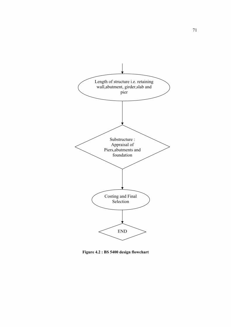
71

END

Costing and Final Selection

Substructure : Appraisal of

Piers,abutments and foundation

Length of structure i.e. retaining wall,abutment, girder,slab and

pier

Figure 4.2 : BS 5400 design flowchart

72

DESIGN FLOWCHART OF PRESTRESSED COMPOSITECONCRETE I GIRDER BRIDGE ACCORDING TO AASHTO

Determine Impact and Distribution Factors

Calculate Moment of Inertia of Composite Section

Calculate Dead Load on Prestressed Girder

Compute Dead Load Moments

Calculate Live Load Plus Impact Moment

Calculate Stresses at Top fiber of Girder

73

Calculate Stresses at Bottom fiber of Girder

Calculate Stresses at Bottom fiber of Girder

Calculate Initial Prestressing Force

Calculate fiber Stresses in Beam

Determine and Check Required Concrete Strength

Define Draping of Tendons

Check Required Concrete Strength

Check Ultimate Flexural Capacity

Finish

Figure 4.3 : Design Flowchart of I Girder Bridge according to AASHTO

74

DESIGN FLOWCHART OF PRESTRESSED COMPOSITECONCRETE I GIRDER BRIDGE ACCORDING TO BS5400

Calculate MomentVariation

(live load + finishes)

Stress limit(Structure class concrete grade)

Min. Section Modulus

Trial Section(Shape,Depth,Web,Flange limit,cover,Loss allowance) Serviceability

L.S

Self weight + dead load mom ent

Total moment

Min. prestress force

75

(Cable zone width limit, max eccentricity)

Design prestress force

Tendon profile

Transfer stresses

Check final stresses

Serviceability L.S

Check deflection

Design end block (Prestress system)

Ultimate mom. of resistance

Untensioned Reinforced

Shear design Ultimate L.S

Finish Check end block (unbonded)

76

Figure 4.4 : Design flowchart of I-Girder Bridge according to BS 5400

ANALYSIS OF COLUMN BENT PIER UNDER SEISMIC LOADING ACCORDING TO AASHTO

Determine Type of Seismic Analysis and Other Criteria

Compute stiffness of the Pier

Compute Load due to Longitudinal Motion

Compute Load due to Transverse Motion

Summarizes Loads Acting On Pier Column

Check for Effects of Slenderness

Compute Moment Magnification Factor

77

Determine Required Reinforcing Steel END

Figure 4.5: Design Flowchart of Column Bent Pier according to AASHTO

ANALYSIS OF COLUMN BENT PIER ACCORDING TO BS 5400

Calculate nominal load

Adopt size of pier -Determine self weight

Design design dowel design capping design column bearing bar beam

design pile cap short column

design as beamdesign piles

Long column

Load determine structural Load at ULS at SLS capacity of piles

Load Load Combination combination

Calculate maximun reaction Type of piles and nos

Check maximun reaction Design pile cap

78

Design load capacity of piles Based on soil data-design length of piles

- Geotechnical capacity

Figure 4.6: Design Flowchart of Column Bent Pier according to BS 5400

DESIGN OF A STUB ABUTMENT WITH SEISMIC DESIGN CODEACCORDING TO AASHTO

Determine Type of seismic Analysis and Other Criteria

Compute Seismic active earth Pressure

Compute Static Active Earth Pressure

Compute Equivalent Pressure

Compute Abutment Loads

Compute Active Earth Pressure for Stemand Wall

Compute Abutment Stiffness

Compute Earthquake Load On Abutment

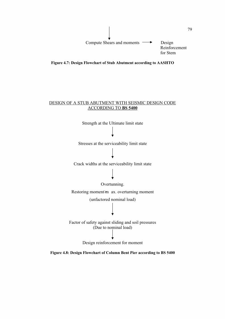
79

Compute Shears and moments DesignReinforcementfor Stem

Figure 4.7: Design Flowchart of Stub Abutment according to AASHTO

DESIGN OF A STUB ABUTMENT WITH SEISMIC DESIGN CODEACCORDING TO BS 5400

Strength at the Ultimate limit state

Stresses at the serviceability limit state

Crack widths at the serviceability limit state

Overtunning.

Restoring moment> m ax. overturning moment

(unfactored nominal load)

Factor of safety against sliding and soil pressures (Due to nominal load)

Design reinforcement for moment

Figure 4.8: Design Flowchart of Column Bent Pier according to BS 5400

80

4.3 Result and Analysis

Table 4.1 and table 4.3 show the va lue of require steel area for

usage of different codes.According to the table, we can see that percentage

of difference steel area for each members that use difference type of

codes.

Codes of Practices

Amount of Steel Area (mm2)

AASHTO BS5400 Percent of Difference

( %) Deck 1341 (H16-150) 1006 (H16-200) 33.30

Girder 7*3039 (4.71 in 2 ) = 21273

7*5400 = 37800

43.72

Column 6*17710 (22H32) =106260

16,905 (21H32) = 101430

4.76

Abutment (Moment Steel + Shear)

2*(7543 + 2095) = 19360

2*(5892)= 11784

64.29

Table 4.1 : Steel Area for different code of practice.Consider for seismic reading 0.15 g

Codes of Practices

Cost of Steel Area (RM2000/tonne)

AASHTO BS5400 Percent of Difference

( %) Deck RM 632 RM 474 33.30

Girder 7*(RM1432)=RM10024

7*(RM2542)= RM17794

43.67

Column 6*(RM 2113) = RM12678

6*(RM 2017) = RM12102

4.76

Abutment (Moment Steel + Shear)

2*(RM 855) = RM1710

2*(RM 647) = RM 1294

32.15

Overall Cost RM 24,412 RM 31664 22.90

Table 4.2 : Cost of steel area for different code.Consider seismic reading 0.15 g

81

Table 4.2 and table 4.4 show the steel area cost for usage of different

codes.According to the table, we can see that percentage of difference

steel area cost for each members that use difference type of codes.

Codes of Practices

Amount of Steel Area (mm2)

AASHTO BS5400 Percent of Difference

( %) Deck 1341 (H16-150) 1006 (H16-200) 33.30

Girder 7*3039= 21273

7*5400= 37800

43.67

Column 6*17710 (22H32) =106260

16,905 (21H32) = 101430

4.76

Abutment (Moment Steel + Shear)

2*(5632 + 1609) = 14482

2*(5892)=11784

22.89

Table 4.3 : Steel Area for different code of practice.Consider for seismic reading 0.075 g

Codes of Practices

Cost of Steel Area (RM2000/tonne)

AASHTO BS5400 Percent of Difference

( %) Deck RM 632 RM 474 33.30

Girder 7*(RM1432)=RM10024

7*(RM2542)= RM17794

42.61

Column 6*(RM 2113) = RM12678

6*(RM 2017) = RM12102

4.76

Abutment (Moment Steel + Shear)

2*(RM 729) =RM 1458

2*(RM 647) = RM 1294

12.67

Overall Cost RM 24792 RM 31664 21.70

Table 4.4 : Cost of steel area for different code.Consider seismic reading 0.075g

82

Graphically Result :

Steel area for different code of practices

0

20000

40000

60000

80000

100000

120000

Am

ou

nt

of

stee

l are

a (m

m^2

)

American Code 1341 21273 106260 19360

British Code 1006 37800 101430 11784

Deck Girder Column Abutment

Figures 4.9 : Steel Area for different code of practice.Consider for seismic reading 0.15 g

Steel area for different code of practices

0

20000

40000

60000

80000

100000

120000

Am

ou

nt

of

stee

l are

a (m

m^2

)

American Code 1341 21273 106260 14482

British Code 1006 37800 101430 11784

Deck Girder Column Abutment

Figures 4.10 : Steel Area for different code of practice.Consider for seismic reading 0.075 g

83

Cost of steel area for 0.15 g seismic reading

0

5000

10000

15000

20000

Co

st (

RM

)

American Code 632 10024 12678 1710

British Code 474 17794 12102 1294

Deck Girder Column Abutment

Figures 4.11 : Cost of steel area for different code.Consider seismic reading 0.15 g

Cost of steel area for 0.075 g seismic reading

0

5000

10000

15000

20000

Co

st (

RM

)

American Code 632 10024 12678 1458

British Code 474 17794 12102 1294

Deck Girder column Abutment

Figures 4.12 : Cost of steel area for different code.Consider seismic reading 0.075g

Meanwhile , table 4.5 and table 4.6 indicated the result of Time

History Analysis in order end member force (Girder) among both codes of

practices.

84

Member Joint Axial(kN)

Shear-Y(kN/m2)

Moment-Z

AxialCapacity

of the Column(MN)

MomentCapacity of

Girder(kN.m)

ShearCapacity of Structure(MN/m2)

1 386.40 74.7 8 156.03 - 9,231.30 3270.301(Girder) 2 -189.51 122.11 -582.05 - 9,231.30 3270.30

2 181.57 162.99 720.80 - 9,231.30 3270.302(Girder) 3 145.49 164. 07 -737.08 - 9,231.30 3270.30

3 -219.48 120.65 564. 28 - 9,231.30 3270.303(Girder) 4 416.37 76.25 -164.6 6 - 9,231.30 3270.30

5 -53.21 98.48 -182.68 2,218.82 3,48 7.764(Column) 2 -53.21 7.94 -138.76 2,218.82 3,48 7.76

6 -56.93 39.87 -43.24 2,218.82 3,48 7.765(Column) 3 -56.93 73.99 172.80 2,218.82 3,48 7.76

Table 4.5 : Time History Analysis due to End Member of Force by using British code analysis (Staad-Pro)

Member Joint Axial(kN)

Shear-Y(kN/m 2)

Moment-Z

AxialCapacity

of the Column(MN)

MomentCapacity of

Girder(kN.m)

ShearCapacity of Structure(MN/m 2)

1 438. 34 86.24 180.89 - 9,231.30 3270.301(Girder) 2 -211.79 140.32 -667.61 - 9,231.30 3270.30

2 208.89 187.63 830.70 - 9,231.30 3270.302(Girder) 3 167.44 188.71 -846.9 1 - 9,231.30 3270.30

3 -246.2 2 138.86 649. 93 - 9,231.30 3270.303(Girder) 4 472. 77 87.70 -189.47 - 9,231.30 3270.30

5 53.21 -103.53 -194.1 6 2,218.82 3,48 7.764(Column) 2 53.21 -2.90 -163.09 2,218.82 3,48 7.76

6 56.93 -35.08 -31.05 2,218.82 3,48 7.765(Column) 3 56.93 -78.77 196.98 2,218.82 3,48 7.76

Table 4.6 : Time History Analysis due to End Member of Force by using American codeanalysis (Staad-Pro)

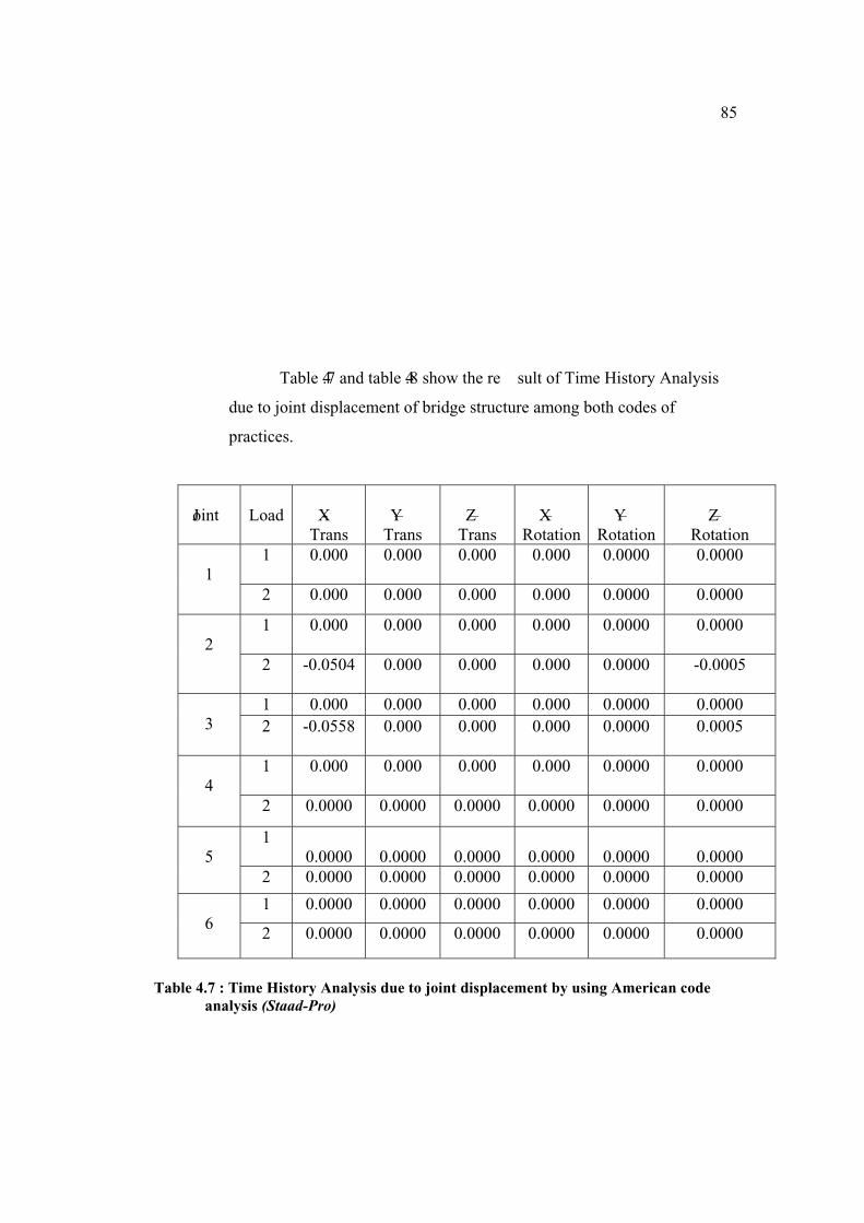
85

Table 4.7 and table 4.8 show the re sult of Time History Analysis

due to joint displacement of bridge structure among both codes of

practices.

Joint Load X - Trans

Y –Trans

Z – Trans

X – Rotation

Y – Rotation

Z – Rotation

1 0.000 0.000 0.000 0.000 0.0000 0.00001

2 0.000 0.000 0.000 0.000 0.0000 0.0000

1 0.000 0.000 0.000 0.000 0.0000 0.00002

2 -0.0504 0.000 0.000 0.000 0.0000 -0.0005

1 0.000 0.000 0.000 0.000 0.0000 0.00003 2 -0.0558 0.000 0.000 0.000 0.0000 0.0005

1 0.000 0.000 0.000 0.000 0.0000 0.00004

2 0.0000 0.0000 0.0000 0.0000 0.0000 0.0000

10.0000 0.0000 0.0000 0.0000 0.0000 0.00005

2 0.0000 0.0000 0.0000 0.0000 0.0000 0.0000

1 0.0000 0.0000 0.0000 0.0000 0.0000 0.00006

2 0.0000 0.0000 0.0000 0.0000 0.0000 0.0000

Table 4.7 : Time History Analysis due to joint displacement by using American code analysis (Staad-Pro)

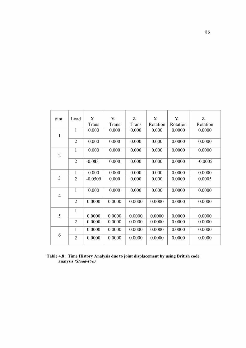
86

Joint Load X - Trans

Y –Trans

Z – Trans

X – Rotation

Y – Rotation

Z – Rotation

1 0.000 0.000 0.000 0.000 0.0000 0.00001

2 0.000 0.000 0.000 0.000 0.0000 0.0000

1 0.000 0.000 0.000 0.000 0.0000 0.00002

2 -0.0483 0.000 0.000 0.000 0.0000 -0.0005

1 0.000 0.000 0.000 0.000 0.0000 0.00003 2 -0.0509 0.000 0.000 0.000 0.0000 0.0005

1 0.000 0.000 0.000 0.000 0.0000 0.00004

2 0.0000 0.0000 0.0000 0.0000 0.0000 0.0000

10.0000 0.0000 0.0000 0.0000 0.0000 0.00005

2 0.0000 0.0000 0.0000 0.0000 0.0000 0.0000

1 0.0000 0.0000 0.0000 0.0000 0.0000 0.00006

2 0.0000 0.0000 0.0000 0.0000 0.0000 0.0000

Table 4.8 : Time History Analysis due to joint displacement by using British code analysis (Staad-Pro)

87

Finally , table 4.9 and table 4.10 show the result of Time history Analysis

due to support reaction among both codes.

Joint Load FORCE- X

FORCE- Y

FORCE- Z

MOM-X

MOM-X

Z – Rotation

1 0.00 0.00 0.00 0.00 0.00 0.001

2 438.34 86.24 0.00 0.00 0.00 180.89

1 0.00 0.00 0.00 0.00 0.00 0.004

2 472.76 87.70 0.00 0.00 0.00 -189.46

1 0.00 0.00 0.00 0.00 0.00 0.005 2 103.53 53.21 0.00 0.00 0.00 -194.16

1 0.00 0.00 0.00 0.00 0.00 0.006

2 35.02 56.89 0.00 0.00 0.00 -30.95

10.00 0.00 0.00 0.00 0.00 0.002

2 0.00 381.16 0.00 0.00 0.00 0.00

1 0.00 0.00 0.00 0.00 0.00 0.003

2 0.00 384.46 0.00 0.00 0.00 0.00

Table 4.9 : Time History Analysis due to support reaction by using American code analysis (Staad-Pro)

88

Joint Load FORCE- X

FORCE- Y

FORCE- Z

MOM-X

MOM-X

Z – Rotation

1 0.00 0.00 0.00 0.00 0.00 0.001

2 961.15 184.36 0.00 0.00 0.00 358.34

1 0.00 0.00 0.00 0.00 0.00 0.004

2 998.93 186.16 0.00 0.00 0.00 -368.59

1 0.00 0.00 0.00 0.00 0.00 0.005 2 106.28 53.21 0.00 0.00 0.00 -199.98

1 0.00 0.00 0.00 0.00 0.00 0.006

2 30.37 56.89 0.00 0.00 0.00 -18.17

10.00 0.00 0.00 0.00 0.00 0.002

2 0.00 806.42 0.00 0.00 0.00 0.00

1 0.00 0.00 0.00 0.00 0.00 0.003

2 0.00 809.69 0.00 0.00 0.00 0.00

Table 4.10 : Time History Analysis due to support reaction by using British code analysis (Staad-Pro)

89

4.13 ) Mode Shape of bridge structure during earthquake event for each codes of practices design

Fig 4.13 a : Mode Shape of bridge structure during earthquake event for American code design

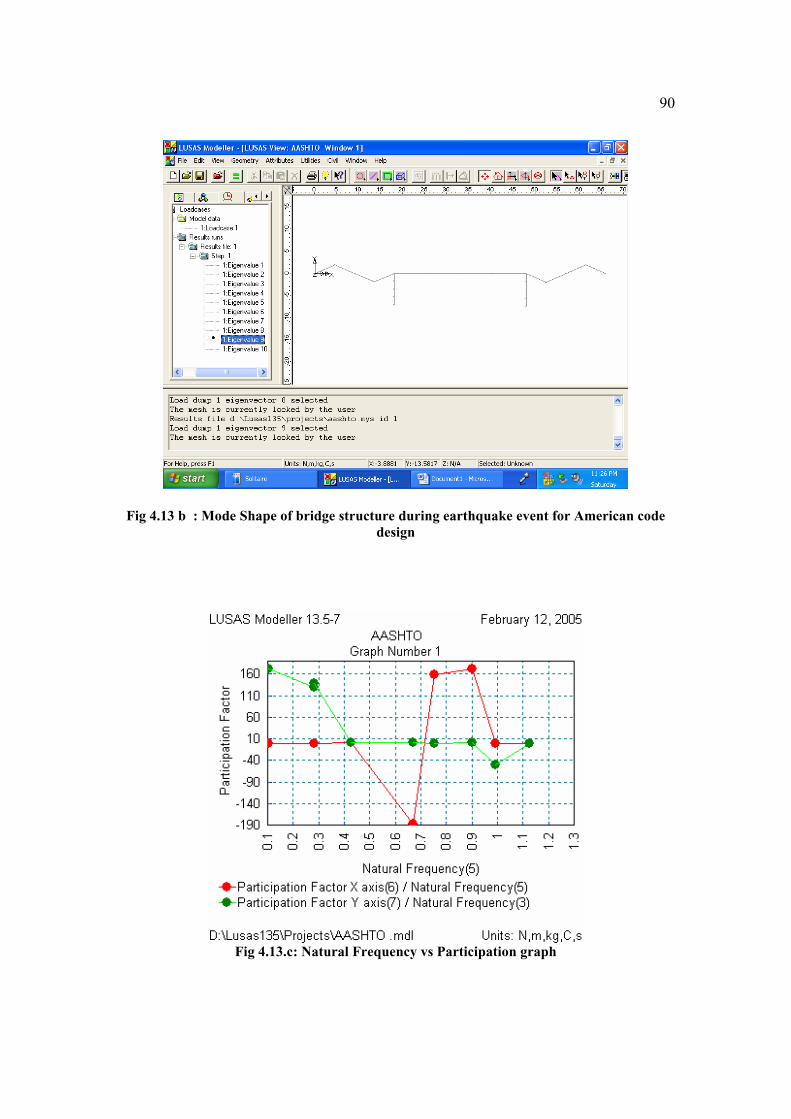
90

Fig 4.13 b : Mode Shape of bridge structure during earthquake event for American code design

Fig 4.13.c: Natural Frequency vs Participation graph

91

0

1

2

3

4

5

6

0 5 10 15 20 25 30 35 40

Period (Sec)

Acc

eler

atio

n (

m/s

ec^2

)

Series1

Fig. 4.13.d : Time History Analysis graph for American code design

Fig 4.14. a : Mode Shape of bridge structure during earthquake event for British code design by using Lusas Software

92

Fig 4.14. b : Mode Shape of bridge structure during earthquake event for British code design by using Lusas Software

Fig 4.14.c. : Natural Frequency vs Participation graph

.

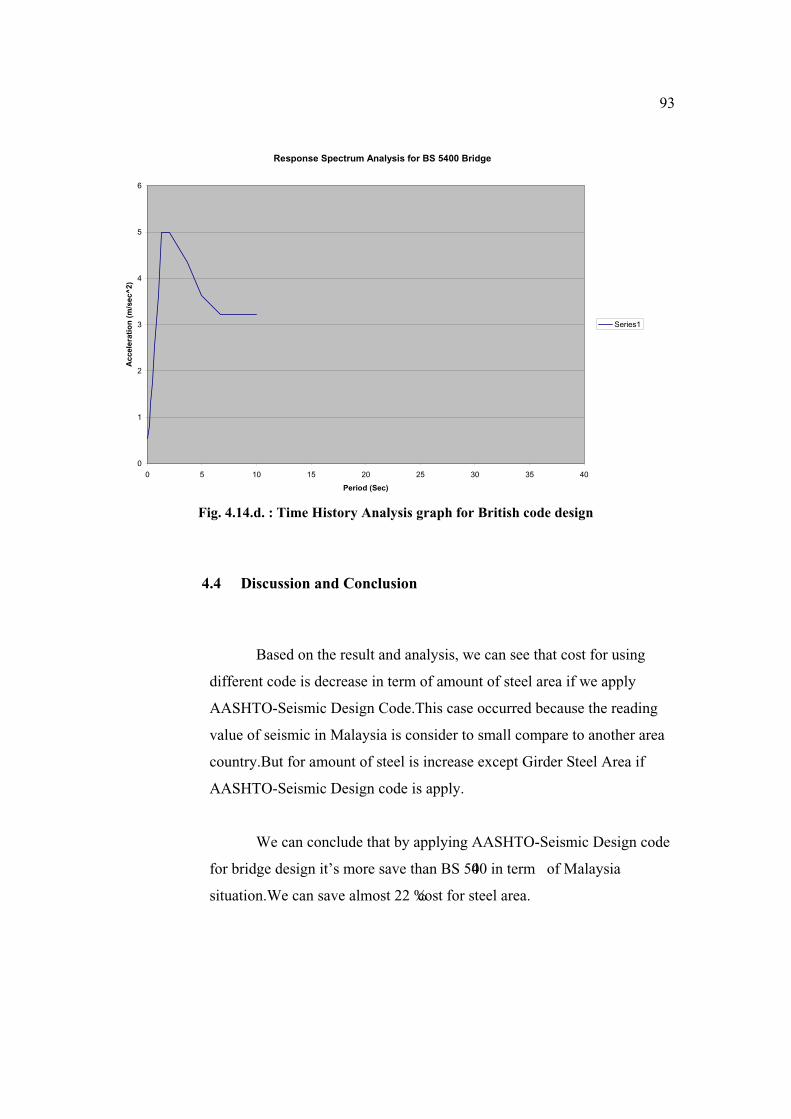
93

Response Spectrum Analysis for BS 5400 Bridge

0

1

2

3

4

5

6

0 5 10 15 20 25 30 35 40

Period (Sec)

Acc

eler

atio

n (

m/s

ec^2

)

Series1

Fig. 4.14.d. : Time History Analysis graph for British code design

4.4 Discussion and Conclusion

Based on the result and analysis, we can see that cost for using

different code is decrease in term of amount of steel area if we apply

AASHTO-Seismic Design Code.This case occurred because the reading

value of seismic in Malaysia is consider to small compare to another area

country.But for amount of steel is increase except Girder Steel Area if

AASHTO-Seismic Design code is apply.

We can conclude that by applying AASHTO-Seismic Design code

for bridge design it’s more save than BS 5400 in term of Malaysia

situation.We can save almost 22 % cost for steel area.

CHAPTER V

CONCLUSION AND SUGGESTION

5.0 Introduction

As we mentioned in last chapter I, our target in comparison

between these both codes are to investigate percentage of cost whether

increase or decrease in term of seismic design consideration in our bridge

in Malaysia.In fact of that, we also make study on behaviour of existing

bridge capacity in Malaysia towards to seismic loading.

We also try find out the level of design strength for our current

bridge design code and new bridge design code (AASHTO-Seismic

Design) that we supposed to invesigate to determine capability in resisting

the seismic loading to bridge structure.

We conduct this study by redesign existing bridge in Malaysia with

a new code of practices.In our case, our new design code that we adopt

and apply is AASHTO-Seismic Design.We redesign all structure

component by manually hand calculation without using any kinds of

software design.This is because, we try understand deeply the application

of seismic design consideration before we perform using software design

i.e LUSAS,Cosmos,SAP 90,Staad-Pro etc.

95

5.1 Future Research

The study of comparison between both different code in our

country toward our bridge in Malaysia is just beginning.There are a lot of

improvement that can be done to get a better and accurate result or

outcome so that we can recover our currently backdraw practice in design

of our bridge structure in Malaysia.We plan to perform this bridge case by

using software design that just concentrate only to seismic loading

independently.We decide to use LUSAS software application in doing our

case study.

5.1.1. Future Challenges in Bridge Engineering

Having given an overview of more than two millennia in bridge

building with some discussion of the impact of developments on later

bridge engineering, the following paragraphs shall look ahead. The second

half of this chapter will give an overview of the wide spectrum of future

challenges. As opposed to the history of bridges, for which an abundance

of literature can be found in any library, books or articles on the future of

bridge construction are more rare.How can predictions be made at all? The

basic approach is to identify current problem areas and trends in research

interests. With some imagination, it is then possible to derive ideas of

where bridge engineering may be heading. These predictions will certainly

not be exact, but they give an impression of future challenges. New

concepts are emerging, yet there is still very little experience with the

practical application of these. It will take creativity and sometimes also

courage to face them.

96

The following sections will outline these areas of challenge for

coming generations of bridge engineers. Three main areas are identified:

Dealing with the engineering approach towards the complete project life-

cycle, including design, construction, maintenance, and rehabilitation;

secondly new or improved materials; and finally new types of structures

are discussed.

5.2 Improvements in Design, Construction, Maintenance, and

Rehabilitation

The construction industry is unique in the way that most of its

structures are one-of-a-kind products. As opposed to industrial

manufacturing, the construction industry in most cases produces structures

that are adapted to the owner’s specific wishes and to constraints imposed

by site conditions and technical possibilities. The processes that lead to the

complete structure are discussed in much more detail in Chapter 3. Here,

some areas of possible improvements shall be pointed out.

5.2.1 Improvements in Design

Since the construction of a real structure is the ultimate goal of all

design, the design process inevitably needs to consider the requirements

and limitations of construction methods. Current issues in improving

design for construction focus on better designs through an increased team

effort of all parties involved. Construction engineering concepts, such as

Design-Build Construction and Partnering all deal with trying to foster

close cooperation and improve communication to achieve better overall

97

project performance.Apart from managerial improvements, especially the

development of prestressed concrete segmental bridges has given

designers a wide range of possibilities at hand. In addition to the

possibilities inherent to this kind of concrete, designers are able to choose

from improved or newly developed materials. More information on high-

performance materials is given in Section 2.2.2. Use of advanced materials

of higher strength, less weight, and improved durability will allow smaller

structural members for substructures and superstructures and less dead

load of the structures that they form. Up to a certain point these

improvements remain well within the classic design methodology, but as

Podolny (1998, p26) writes, with enhanced materials and new structural

concepts necessity can arise “to deal with new limit states, such as user

sensitivity to vibration or claustrophobic reaction to long tubular structures

or tunnels.” With these advanced materials in innovative structures, the

center of attention may shift even more to the serviceability of the

structures. Podolny and Muller (1982) state that at some time a situation is

reached where stress criteria are not determining anymore, but are

overruled by limitations to deformations. They also point at the increased

necessity to examine special failure modes of slender, yet strong structural

members, such as buckling. Fabrication tolerances would have to be

included in these considerations.In the past two decades, the enormous

development of computer capabilities has certainly provided engineers

with much better tools for performing a vast amount of analytical

calculations in very short time. Still, it has to be cautioned about too much

relying on computer results and the models on which they are based.

5.2.2 Improvements in Construction

The core issues governing the actual construction process are

safety and economy, with the latter one referring especially to a smooth

98

construction process on budget and within time scheduled. Quality control

is necessary to ensure that the structure and its parts are built according to

the specifications. Control of all these goals is the main task of

construction management.Depending on the actual construction method

employed to the specific project, various ways of simplifying and

speeding up construction works for economy exist. Examples provided in

technical literature are e.g. increased use of precast elements to speed up

construction on site, such as prefabricating webs for cast-in-place box

girders (Mathivat 1983). Podolny and Muller (1982) give an example of a

modified method of incremental launching, where the concrete deck for a

steel superstructure is cast and launched forward stepwise, thus reducing

the need for formwork considerably. More methods of combining different

erection methods and implementing both precast and cast-in-place

segments where advantageous are conceivable. In future, introduction of

more automated equipment on site can help accomplish certain repetitive

tasks. The uniqueness and complex conditions of every site, as well as the

multitude of tasks to be performed during construction yet still make such

automation very difficult. Use of improved equipment, e.g. modular

formwork and shoring systems, are but small steps towards the goals

outlined above.

5.2.3 Improvements in Maintenance and Rehabilitation

Bridges have to withstand a large variety of environmental

influences during their service life.The natural environment induces

stresses in the structure e.g. through temperature gradients.Strong winds,

flood events and seismic events put the structural stability and integrity to

a test.Corrosive chemicals in water and air, as well as present through

99

deicing agents for roadways affect the soundness of the materials.

Dynamic loads from traffic and winds generate fatigue.Construction

details, as e.g. joints, bearings, and anchorages suffer from wear and tear.

Apart from these influences various forms of impact, e.g. from passing

vehicles or ship traffic need to be anticipates in design of the structure.

Maintenance of bridges comprises regular inspections, renewal of e.g.

protective exterior coatings, replacement of parts as e.g. worn out bridge

bearings, and other minor repairs. A certain percentage of total

construction cost is commonly budgeted for annual maintenance of

bridges under service. Inspections are required in order to keep informed

on the current state of the bridge. Future development of technical systems

could support or even replace these inspections. Sensors built into the

structure could then be used to measure the current state of deterioration,

e.g. in the bridge deck and to detect weaknesses. Links with computer

databases and software for so-called bridge management systems could

then help interpreting the data collected. Accessing these data will allow

for decisions as to the measures required to keep the structure at a

serviceable condition. Measures that simplify construction work can also

make repair and rehabilitation work easier.

Modularization of structural members and good accessibility of the

whole assembly will contribute to performing repair and rehabilitation

work with greater ease. Structural details affected by wear and tear and

thus most susceptible to corrosion are traditionally bearings and joints.

Reducing the number of complicated details and focussing efforts on good

detailing of these will contribute to a longer service life of the whole

structure. Good design will also anticipate easy replacement of these parts.

Another most important factor for the length of bridge service life

is materials. Less weight of structural members due to stronger materials

will simplify handling these members. Workability is another factor that

100

can determine the high performance of a material. In the area of materials

for repair and rehabilitation development of coatings, epoxy grouts, fiber

reinforcement, and other materials enables the repairs to be very specific

adapting to the problem.

5.3 Conclusion

With the prospects and possibilities presented above one can say

that the future of bridges has just begun. The three main areas of future

development that were pointed out in the previous sections show that the

range of ideas to be explored is very wide. Some of these ideas may prove

impractical within the technical environment, while others will become

feasible once the existing technologies have been developed further. The

approaches mentioned will contribute to the development of amazing new

structures. Only the fascination that is characteristic for bridge engineering

field will remain the same that it has always been, during the many

centuries that have passed since the first bridges were erected.

REFERENCES

Standard Specifications for Highway Bridges, 15th ed, American Association

of State highway and Transportation Officials, Washington, D.C, 1993.

Standard Plans for Highway Bridges, vol. I,Concrete Superstructures, U.S

department of Transportation ,Federal Highway Administration,Washington,

D.C,1990.

Winter,George and Nolson,Arthur H., Design of Concrete Structures, 9th

ed.,McGraw-Hill,New York,1979.

Gutkowski,Richard M. and Williamson,Thomas G., “Timber Bridges:State of

Art,” Journal of Structural Engineering,American Society of Civil

Engineers,pp.2175-2191,vol.109,No.9,September,1983.

Standard details for Highway Bridges,New york State Deparment of

Transportation,Albany,1989.

Elliot,Arthur L.,”Steel and Concrete Bridges,”Structural Engineering

Handbook,Edited by Gaylord,Edwin H., Jr., and Gaylord,Charles N.,

McGraw-Hill,New York,1990.

AASHTO Manual for Bridge Maintenance,American Association of State

Highway and Transportation Officials,pp.77-104,Washington,D.C.,1987.

Bridge Design Practice Manual,CaliforniaDepartment of Transportation,p.1-

11,Sacramento,1983.

102

Robert A.et al., Goals,Opportunities, and Priorities for the USGSEartquake

Hazard Reduction Program,U.S. geological Survey,p.366,Wahington,

D.C.,1992.Bridge Design Practice Manual, 3rd ed., California Department of

Transportation, Sacramento.,1971.

Steinman ,D.B., and Watson , S.R., Bridges and Their Builders,2nd ed., Dover

Publications Inc., New York,1957.

Starzewski,K., “Earth Reatining Structures and Culverts.”The Design and

Construction of Engineering Foundation,Edited by Hendry, F.D.C.,

Chapman and Hall, New York, 1986.

Bowles,Joseph E., Foundation Analysis and Design, 2 nd ed., McGraw-

Hill,New York,1977.

Standard Specification for Highway Bridges, 15th ed., American

Association of State Highway and Transportation Officials, p. 646,

Washington, D.C., 1993.

Walley,W.J., and Purkiss, J.A., “Bridge Abutment and Piers,” pp. 821 –

884,The Design and Construction of Engineering Foundations,Edited by

Henry, F.D.C., Chapman and Hall, New York, 1986.

Standard Specifications for Highway Bridges, 15th ed, American

Association of State highway and Transportation Officials, Washington,

D.C, 1993.

Standard Specifications for Highway Bridges, 15th ed, American

Association of State highway and Transportation Officials,

Washington,pp. 646 D.C, 1993.

103

Winter , George, and Nilson, Arthur H., Design of Concrete Structures,9th

ed.,McGraw-Hill,New York,1979.

APPENDIX A

Design of reinforced concrete deck slab

Problem : Design the transversely reinforced concrete deck slab.

Given :

1. Bridge to carry two traffic lanes.

2. Bridge loading specified to be HS20-44.

3. Concrete strength fc’ = 4,500 psi = C40

4. Grade 60 reinforcement fs = 24,000 psi

5. Account for 25 psf future wearing surface.

6. Deck has integrated wearing surface.

Step 1 : Compute the Effective Span Length

From table 3.6 (AASHTO) effective span length criteria for concrete slabs,for a slab

supported on concrete stringer and continuous over more than two longitudinals supports:

S = Clear Span (Clear distances between faces of supports)

= 5.75 ft

Step 2 : Compute Moment due to Dead Load

Dead load includes slab and future wearing surfaces,so that the total dead load on the slab

is

DL = (thickness of slab)(Weight of concrete ) + Future WS

= [(8 in)(1 ft/12 in)(150 Ib/ft3) + (25 Ib/ft2)](1 ft Strip)

= 125.0 Ib /ft.

MDL = 10

2WS =

10

ft)75 Ib/ft)(5.(125.0 2

= 0.41 ft-kips

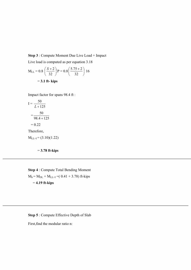
Step 3 : Compute Moment Due Live Load + Impact

Live load is computed as per equation 3.18

MLL = 0.8 32

2SP = 0.8

32

275.5 16

= 3.1 ft- kips

Impact factor for spans 98.4 ft :

I = 125

50

L

=1254.98

50

= 0.22

Therefore,

MLL+I = (3.10)(1.22)

= 3.78 ft-kips

Step 4 : Compute Total Bending Moment

Mb = MDL + MLL+I =( 0.41 + 3.78) ft-kips

= 4.19 ft-kips

Step 5 : Compute Effective Depth of Slab

First,find the modular ratio n:

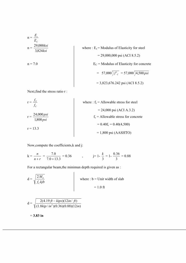
n = C

s

E

E

n = ksi

ksi

824,3

000,29 where : Es = Modulus of Elasticity for steel

= 29,000,000 psi (ACI 8.5.2)

n = 7.0 EC = Modulus of Elasticity for concrete

= 57,000 Cf ' = 57,000 psi500,4

= 3,823,676.242 psi (ACI 8.5.2)

Next,find the stress ratio r :

r = C

S

f

fwhere : fs = Allowable stress for steel

= 24,000 psi (ACI A.3.2)

r = psi

psi

800,1

000,24 fc = Allowable stress for concrete

= 0.40fc = 0.40(4,500) r = 13.3

= 1,800 psi (AASHTO)

Now,compute the coefficients,k and j:

k = rn

n =

3.130.7

0.7 = 0.36 , j= 1-

3

k = 1-

3

36.0 = 0.88

For a rectangular beam,the minimun depth required is given as :

d = kjbf

M

C

b2where : b = Unit width of slab

= 1.0 ft

d = )12)(88.0)(36.0)(/8.1(

)/12)(19.4(22 ininkip

ftinkipsft

= 3.83 in

Step 6 : Compute Required Main Reinforcement

DACTUAL = 7.87 slab- 1.96 Integral W.S – 1.96 cover-(0.75Dia/2) = 3.58 < 3.83 in minimun

Therefore, use d = 4.0 in

AS = jdf

M

Ss

b

= )0.4)(88.0)(24(

)/12)(.19.4(

inksi

ftinkft

= 0.60 in2 /ft = 1,267 mm2/m

Step 7 : Determine number of Bars and Spacing

From predefined tables (see Appendix) we can select various numbers of bars at a given spacing.

Therefore,use # 4 @ 3.5 in- spacing( 0.50 in Dia) = 0.67 in2 / ft

Or H16-125 (1609 mm2)

Step 8 : Compute Distribution Steel in Bottom of Slab

D = S

220=

75.5

220= 91.7 % > 67% so use

Distribution Steel = (AS)(67 %) = (0.22 in2 / ft)(0.67) = 0.15 in2 / ft

Use # 3 @ 8 in-spacing (0.375 in Dia) = 0.17 in2 / ft

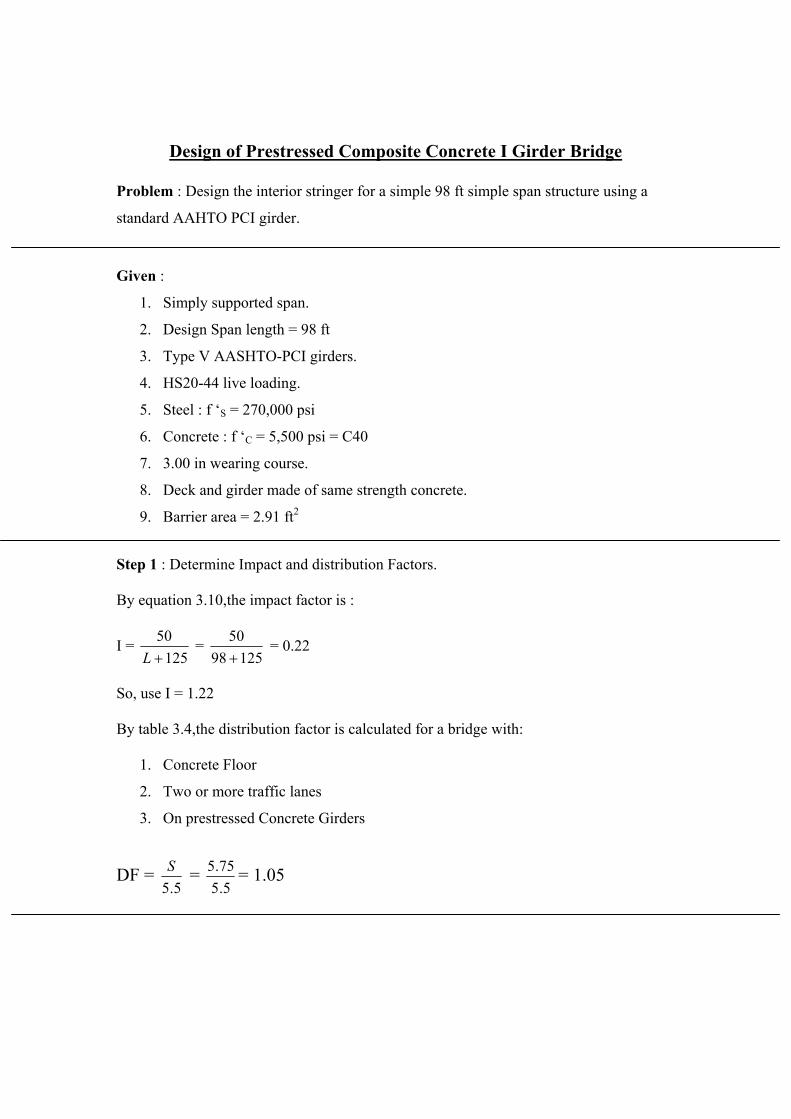
Design of Prestressed Composite Concrete I Girder Bridge

Problem : Design the interior stringer for a simple 98 ft simple span structure using a

standard AAHTO PCI girder.

Given :

1. Simply supported span.

2. Design Span length = 98 ft

3. Type V AASHTO-PCI girders.

4. HS20-44 live loading.

5. Steel : f ‘S = 270,000 psi

6. Concrete : f ‘C = 5,500 psi = C40

7. 3.00 in wearing course.

8. Deck and girder made of same strength concrete.

9. Barrier area = 2.91 ft2

Step 1 : Determine Impact and distribution Factors.

By equation 3.10,the impact factor is :

I = 125

50L

= 12598

50 = 0.22

So, use I = 1.22

By table 3.4,the distribution factor is calculated for a bridge with:

1. Concrete Floor

2. Two or more traffic lanes

3. On prestressed Concrete Girders

DF = 5.5

S = 5.5

75.5 = 1.05

Step 2 : Calculate Moment of Inertia of Composite Section

ELEMENT A (in2) Y (in) AY (in3) AY2 (in4) IO (in4)SLAB 543.0 66.94 36348.42 2433163.235 2798.74GIRDER 1013.0 31.96 32375.48 1034720.34 521,180TOTALS 1556.00 98.90 68723.9 3467883.58 523978.74

IZ = + = 523978.74 + 3467883.58 = 3991862.32 inOI 2AY 2

Y’=A

AY =00.155690.68723 = 44.17 in

I = IZ – ( )( )A 'Y 2 = 3991862.32 – (1556)(44.17)2 = 956123.59 in4

7.87 in thickness of slab

+ C.G SECTION 63”44.17 in

+ C.G GIRDERe = 27.96 in 31.96 in

Assumed C.G PS Force

+ 4.0 in

Step 3 : Calculate Dead Load on Prestressed Girder

The dead load is composed of the following items :

DL slab = (beff)(Slab thickness)(wConc)

= (5.75)(7.87 in)(1 ft/12 in)(0.150 k/ft3) = 0.566 k/ft

DL haunch = (Haunch width)( Haunch thickness)(Wconc)

= (1.33 ft)(1 in)(1 ft/12 in)(0.150 k/ft3) = 0.017 k/ft

DLGIRDER = (girder area)(Wconc)

= (1013 in2)(1 ft/144 in2)(0.150 k/ft3) = 1.06 k/ft

DL Barrier = (2 barriers)(barrier area)(wConc)/7

= (2)(2.61 ft2)(0.150 k/ft3)/7 = 0.11 k/ft

DL Wearing = (W.C thickness)(1/12 ft)(pave.width)(W pave)/7

= (2.0 in)(1ft/12in)(34.4 ft)(0.150 k /ft3)/7 = 0.12 k/ft

Step 4 : Compute Dead Load Moments

Dead Load moments by equation:

Mslab = 8

2WL =8

)0.98)(017.0566.0( ft = 700.0 ft-k

Mgirder = 8

2WL =8

)0.98)(/06.1( 2ftk =1272.5 ft-k

Mbarrie = 8

2WL =8

)0.98)(/157.0( 2ftftk = 188.5 ft-k

Mwearing = 8

2WL =8

)98)(/12.0( 2ftftk =144.06 ft-k

Total MDL = 2305.06 ft-k

Step 5 : Calculate Live Load Plus Impact Moment from figure below,

We locate the HS20-44 truck as shown below:

C/L

16 k 2’4” 4 k 14 ‘0” 16 k

11’8”

BearingA Bearing 49’ 49’ B

98.0 ft

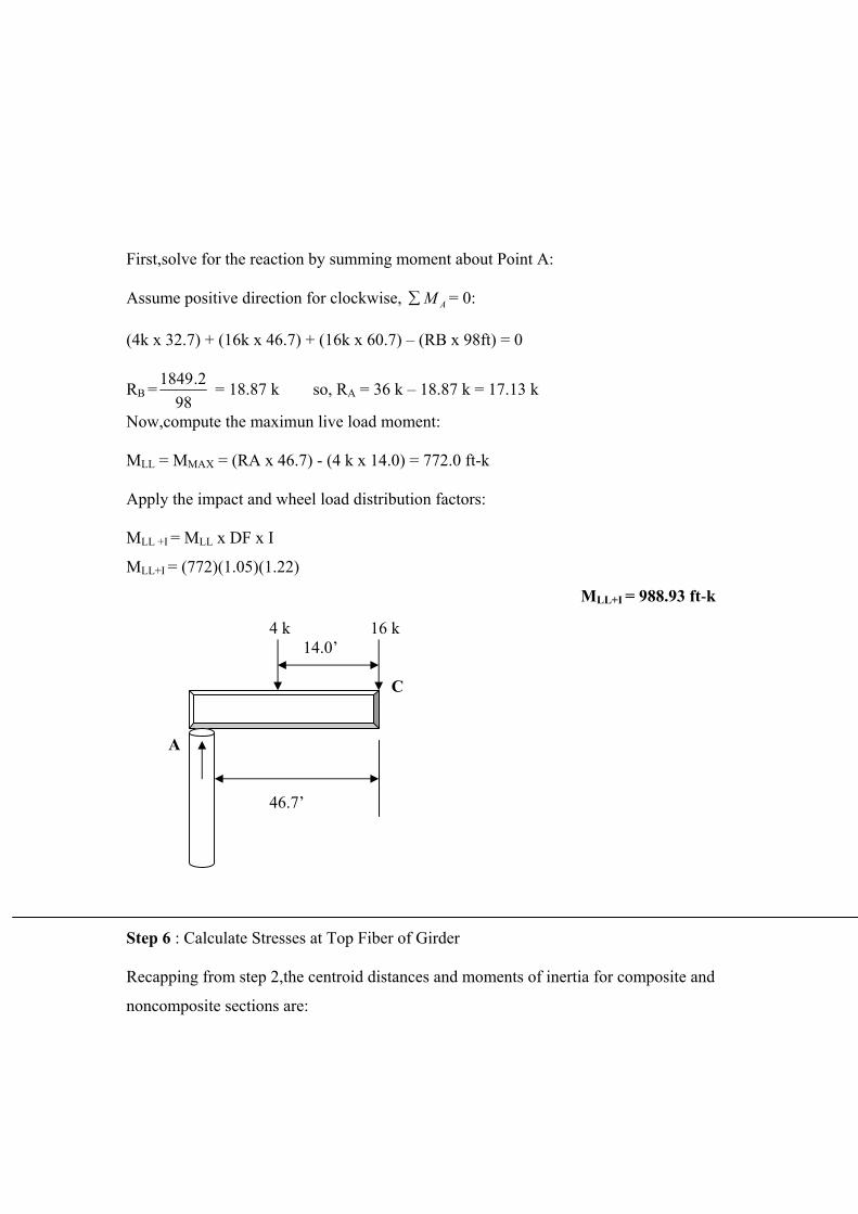
First,solve for the reaction by summing moment about Point A:

Assume positive direction for clockwise, AM = 0:

(4k x 32.7) + (16k x 46.7) + (16k x 60.7) – (RB x 98ft) = 0

RB =98

2.1849 = 18.87 k so, RA = 36 k – 18.87 k = 17.13 k

Now,compute the maximun live load moment:

MLL = MMAX = (RA x 46.7) - (4 k x 14.0) = 772.0 ft-k

Apply the impact and wheel load distribution factors:

MLL +I = MLL x DF x I

MLL+I = (772)(1.05)(1.22)

MLL+I = 988.93 ft-k

4 k 16 k 14.0’

C

A

46.7’

Step 6 : Calculate Stresses at Top Fiber of Girder

Recapping from step 2,the centroid distances and moments of inertia for composite and

noncomposite sections are:

NONCOMPOSITE

Type III Girder

COMPOSITE

7.87 ” Slab & Type III Girder

I = 521,180 in4 956123.59 in4

YT = (63-31.96)in = 31.04 in YT = (63-44.17)in = 18.83 in

31.96 in 44.17 in

The stresses at the top fiber of the girder is calculated using the standard expression

defined by equation (fC = Mc / I):

Element Equation Top Fiber

Slab4521180

)04.31)(/12)(0.700(in

ftin = 0.50NonComposite

Type III

Girder4521180

)04.31)(/12)(5.1272(in

ftin = 0.91

LL + I 459.956123

)83.18)(/12)(989(in

ftin = 0.23

Barrier459.956123

)83.18)(/12)(189(in

ftin = 0.045

Composite

Wearing

Course459.956123

)83.18)(/12)(145(in

ftin = 0.034

Total

fTOP = 1.719 ksi

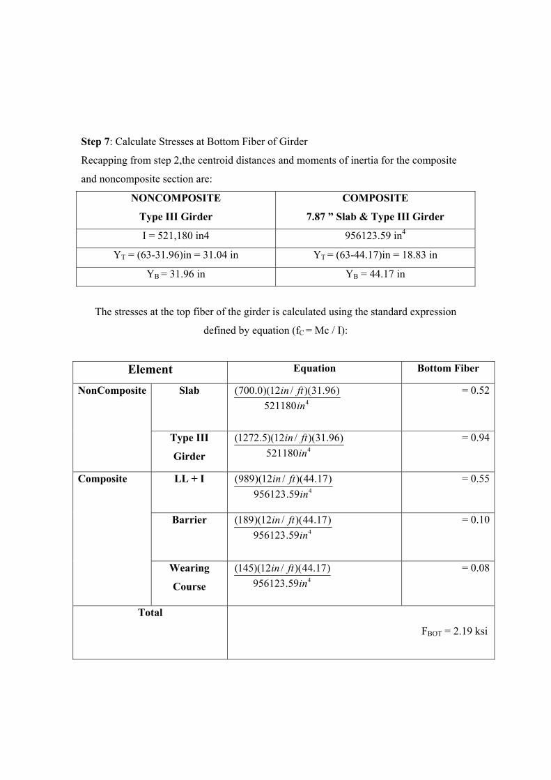
Step 7: Calculate Stresses at Bottom Fiber of Girder

Recapping from step 2,the centroid distances and moments of inertia for the composite

and noncomposite section are:

NONCOMPOSITE

Type III Girder

COMPOSITE

7.87 ” Slab & Type III Girder

I = 521,180 in4 956123.59 in4

YT = (63-31.96)in = 31.04 in YT = (63-44.17)in = 18.83 in

YB = 31.96 in YB = 44.17 in

The stresses at the top fiber of the girder is calculated using the standard expression

defined by equation (fC = Mc / I):

Element Equation Bottom Fiber

Slab4521180

)96.31)(/12)(0.700(in

ftin = 0.52NonComposite

Type III

Girder4521180

)96.31)(/12)(5.1272(in

ftin = 0.94

LL + I 459.956123

)17.44)(/12)(989(in

ftin = 0.55

Barrier459.956123

)17.44)(/12)(189(in

ftin = 0.10

Composite

Wearing

Course459.956123

)17.44)(/12)(145(in

ftin = 0.08

Total

FBOT = 2.19 ksi

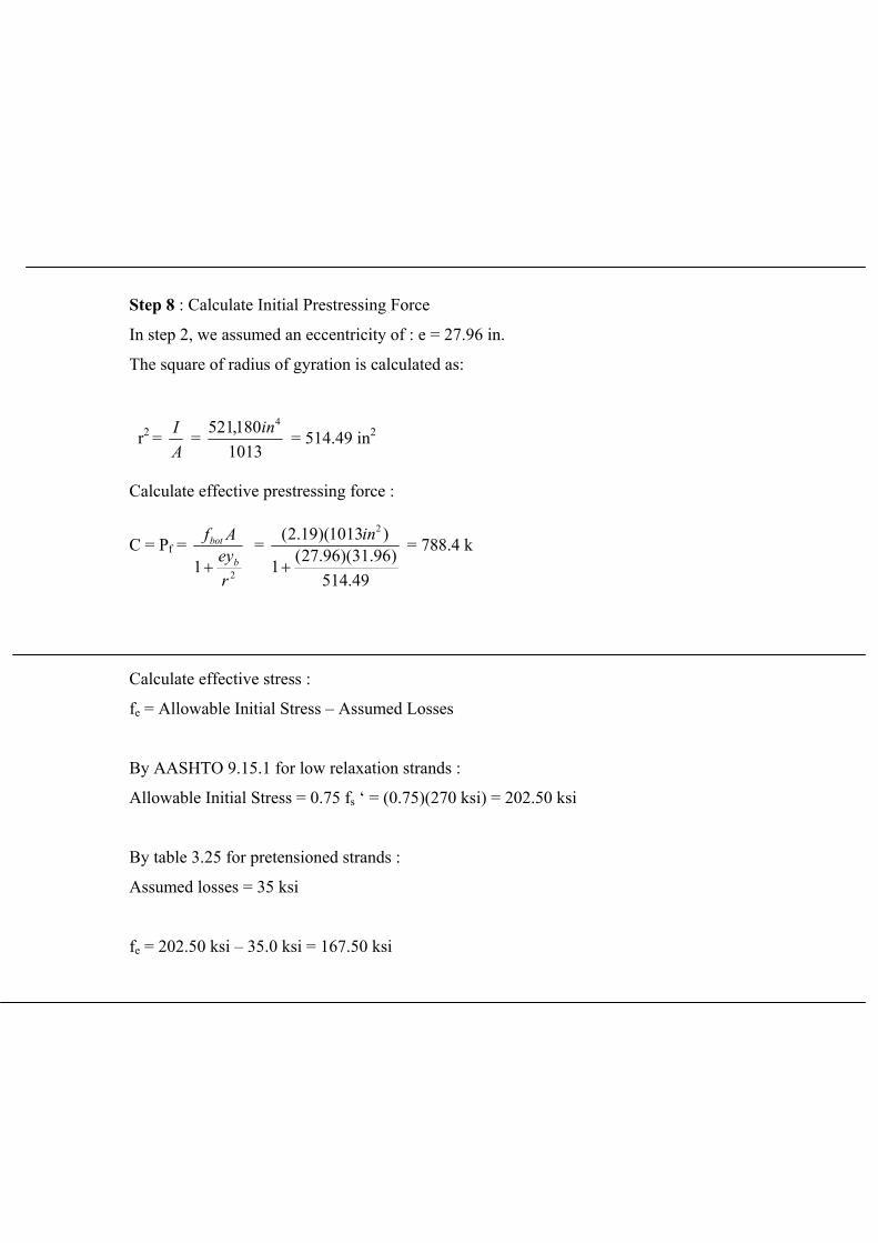
Step 8 : Calculate Initial Prestressing Force

In step 2, we assumed an eccentricity of : e = 27.96 in.

The square of radius of gyration is calculated as:

r2 =A

I = 1013180,521 4in = 514.49 in2

Calculate effective prestressing force :

C = Pf = 21

r

eyAf

b

bot =

49.514)96.31)(96.27(1

)1013)(19.2( 2in = 788.4 k

Calculate effective stress :

fe = Allowable Initial Stress – Assumed Losses

By AASHTO 9.15.1 for low relaxation strands :

Allowable Initial Stress = 0.75 fs ‘ = (0.75)(270 ksi) = 202.50 ksi

By table 3.25 for pretensioned strands :

Assumed losses = 35 ksi

fe = 202.50 ksi – 35.0 ksi = 167.50 ksi

Calculate area of steel:

AS =e

f

f

P =

ksi

k

5.1674.788 = 4.71 in2

Assume losses due to elastic shortening , So:

Losses After Transfer = 35 ksi- 13 ksi = 22 ksi

The initial prestressing force is:

Pi = Pf + (Losses After Transfer)(AS) = 788.4 k + (22 ksi)(4.71 in2)

PI = 892.02 k

Step 9 : Calculate Fiber Stresses in Beam

Compute stresses at top and bottom using equation:

TOP FIBER BOTTOM FIBER

1 + 2r

eyt 1 + 2r

eyb

1 + 49.514

)04.31)(96.27( = -0.67 1 + 49.514

)96.31)(96.27( = 2.74

fTOP = -0.67 A

P +/- ftime fBOT = 2.74 A

P +/- ftime

Time of Stress Equation Stress

At time of prestressing -0.67x 21013

02.892in

k - 0.91 = -0.32 ksi T

At time slab is placed -0.67x 21013

4.788in

k -1.41 = -0.89 ksi C

TopFiber

At design load -0.67x 210134.788

in

k - 1.719 = -1.20 ksi CAt time of

prestressing 2.74 x 2101302.892in

k + 0.94 = - 1.47 ksi C

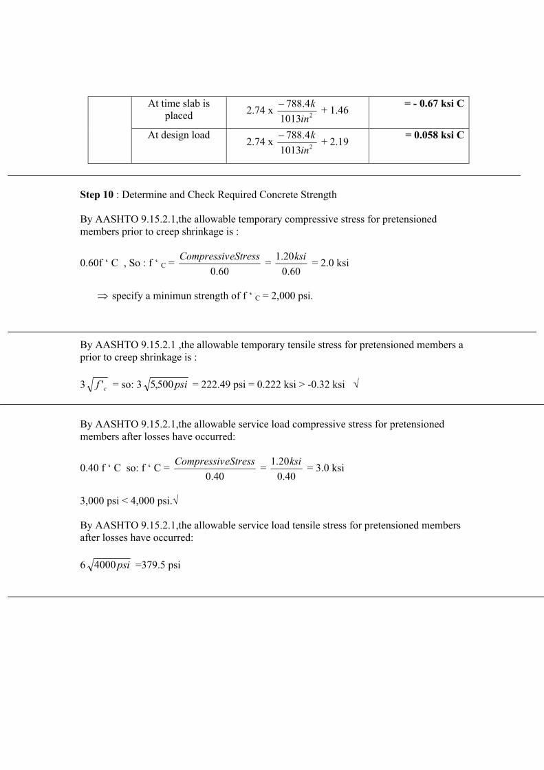
At time slab is placed 2.74 x 21013

4.788in

k + 1.46 = - 0.67 ksi C

At design load 2.74 x 210134.788

in

k + 2.19 = 0.058 ksi C

Step 10 : Determine and Check Required Concrete Strength

By AASHTO 9.15.2.1,the allowable temporary compressive stress for pretensioned members prior to creep shrinkage is :

0.60f ‘ C , So : f ‘ C = 60.0

eStressCompressiv = 60.0

20.1 ksi = 2.0 ksi

specify a minimun strength of f ‘ C = 2,000 psi.

By AASHTO 9.15.2.1 ,the allowable temporary tensile stress for pretensioned members a prior to creep shrinkage is :

3 cf ' = so: 3 psi500,5 = 222.49 psi = 0.222 ksi > -0.32 ksi

By AASHTO 9.15.2.1,the allowable service load compressive stress for pretensioned members after losses have occurred:

0.40 f ‘ C so: f ‘ C = 40.0

eStressCompressiv = 40.0

20.1 ksi = 3.0 ksi

3,000 psi < 4,000 psi.

By AASHTO 9.15.2.1,the allowable service load tensile stress for pretensioned membersafter losses have occurred:

6 psi4000 =379.5 psi

Step 11 : Define Draping of Tendons

Drape tendon with two holddown positions as illustrated below:

L/3=32.7 ‘ L/3=32.7 ‘ L/3=32.7 ‘

A B

Moment at third point moment to midspan moment is then:

MX = 2

)( XLWX at X = 3L : M

3L

X =

23L

W( L – L/3) =

9

2WL

The ratio of third point moment to midspan moment is then :

MMID = 8

2WL so : 2

2

8/9/

WL

WL = 98 = 0.89

Compare this to the ratio of live load moments at L/3 and midspan:

AM = 0:

46.7 ‘

32.7 ‘

18.7 ‘

98.0 ‘ RA RB

( 4 x 18.7) + ( 16 x 32.7) + (16 x 46.7) – ( RB x 98)

RB = 13.73 k RA = 36 – 13.73 = 22.27 k

M = (R3/lx A x 32.7) – (4k x 14 ft) = 664.23 ft-k

The maximun moment (near midspan) calculated earlier in step 5 was found earlier to be

: MMAX = 772.0 ft-k

The ratio of third point to midpoint moments can be taken as :

kft

kft

0.77223.664 = 0.86 Since this is relatively close to 0.89 we will use 0.89 as our

multiplier.

Step 12 : Fiber stresses at Third Points of Beam

The multiplier is applied to the “time dependant” stresses calculated in steps 6 and 7.

Time of Stress Equation Stress

At time of prestressing -0.67x 21013

02.892in

k - (0.91)(0.89) = -0.22 ksi T

At time slab is placed -0.67x 21013

4.788in

k -(1.41)(0.89) = -0.73 ksi C

TopFiber

At design load -0.67x 210134.788

in

k - (1.719)(0.89) = -1.01 ksi CAt time of

prestressing 2.74 x 2101302.892in

k + (0.94)(0.89) = - 1.57 ksi CAt time slab is

placed 2.74 x 210134.788

in

k + (1.46)(0.89) = - 0.83 ksi C

BottomFiber

At design load 2.74 x 210134.788

in

k + (2.19)(0.89) = -0.18 ksi C

Step 13 : Check Required Concrete Strength

By AASHTO 9.15.2.1, the allowable temporary compressive stress for pretensioned

members prior to creep shrinkage is :

0.60 f ‘C so : f ‘C = 60.0

eStressCompressiv = 60.0

57.1 ksi = 2.62 ksi < 4.0 ksi

By AASHTO 9.15.2.1,the allowable temporary tensile stress for pretensioned members

prior to creep shrinkage is :

3 Cf ' = 3 500,5 = 222.49 psi = 0.1897 ksi > -0.22 ksi

This does satisfy the requirement AASHTO 9.15.2.1 specifies,however,that bonded

reinforcement may be provided to resist the total tension in concrete provided that:

Maximun Tensile Stress < 7.5 Cf '

7.5 psi500,5 = 556.21 psi so : -220 psi < 556.21 psi

Determine the number of conventional reinforcing bars required :

Distances to Neutral Axis = psipsi

psiin

1570220)220)(63( = -10.3 in

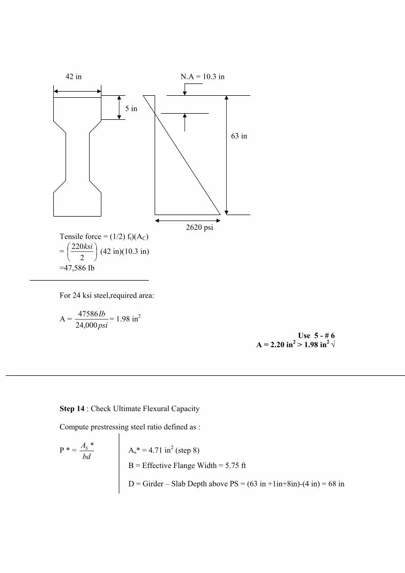
42 in N.A = 10.3 in

5 in

63 in

2620 psiTensile force = (1/2) ft)(AC)

=2

220ksi (42 in)(10.3 in)

=47,586 Ib

For 24 ksi steel,required area:

A = psi

Ib

000,2447586 = 1.98 in2

Use 5 - # 6 A = 2.20 in2 > 1.98 in2

Step 14 : Check Ultimate Flexural Capacity

Compute prestressing steel ratio defined as :

P * = bd

AS * As* = 4.71 in2 (step 8)

B = Effective Flange Width = 5.75 ft

D = Girder – Slab Depth above PS = (63 in +1in+8in)-(4 in) = 68 in

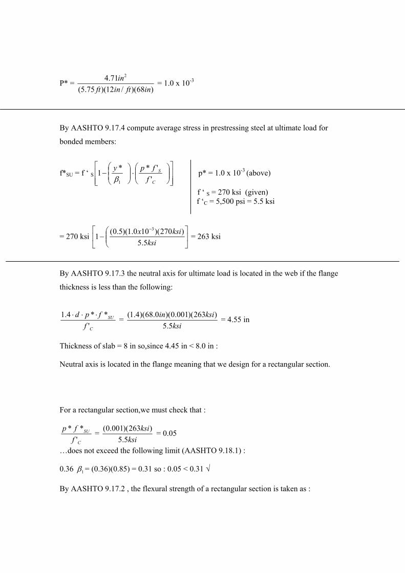
P* = )68)(/12)(75.5(

71.4 2

inftinft

in = 1.0 x 10-3

By AASHTO 9.17.4 compute average stress in prestressing steel at ultimate load for

bonded members:

f*SU = f ‘ SC

S

f

fpy

''**1

1

p* = 1.0 x 10-3 (above)

f ‘ S = 270 ksi (given) f ‘C = 5,500 psi = 5.5 ksi

= 270 ksi ksi

ksix

5.5)270)(100.1)(5.0(1

3

= 263 ksi

By AASHTO 9.17.3 the neutral axis for ultimate load is located in the web if the flange

thickness is less than the following:

C

SU

f

fpd

'**4.1 =

ksi

ksiin

5.5)263)(001.0)(0.68)(4.1( = 4.55 in

Thickness of slab = 8 in so,since 4.45 in < 8.0 in :

Neutral axis is located in the flange meaning that we design for a rectangular section.

For a rectangular section,we must check that :

C

SU

f

fp

'** =

ksi

ksi

5.5)263)(001.0( = 0.05

…does not exceed the following limit (AASHTO 9.18.1) :

0.36 1 = (0.36)(0.85) = 0.31 so : 0.05 < 0.31

By AASHTO 9.17.2 , the flexural strength of a rectangular section is taken as :

C

SUSUSn f

fpdfAM

'**6.01**

nM =ftin

xinin

/1205.06.01)(68)(263(71.40.1 2

= 6809 ft-k

Taking the moment defined by the load factored group loading (see Table 3.2):

M= ][ ILLILLDLDL MM

Using the dead load moment determined in step 4 and the live load plus impact moment

found in step 5 :

M = 1.3[(1.0)(2305.06 ft-k) + (1.67)(989 ft-k)] = 5144 ft-k

So,since we are O.K since we have :

5144 ft-k < 6809 ft-k

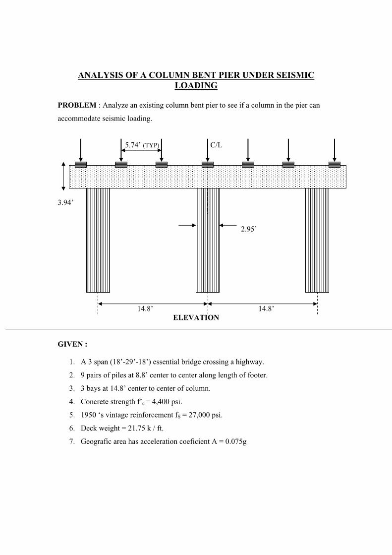
ANALYSIS OF A COLUMN BENT PIER UNDER SEISMICLOADING

PROBLEM : Analyze an existing column bent pier to see if a column in the pier can

accommodate seismic loading.

5.74’ (TYP) C/L

3.94’

2.95’

14.8’ 14.8’ELEVATION

GIVEN :

1. A 3 span (18’-29’-18’) essential bridge crossing a highway.

2. 9 pairs of piles at 8.8’ center to center along length of footer.

3. 3 bays at 14.8’ center to center of column.

4. Concrete strength f’c = 4,400 psi.

5. 1950 ‘s vintage reinforcement fS = 27,000 psi.

6. Deck weight = 21.75 k / ft.

7. Geografic area has acceleration coeficient A = 0.075g

Step 1 : Determine Type of Seismic Analysis and Other Criteria

For an “essential bridge” by AASHTO 3.3 I-A we have:

IC = Importance Classification = I

With an importance classification of “I” by AASHTO 3.4 I-A for :

0.09 < A < 0.19 and IC = I

SPC = Seismic Performance Category = B

The bridge has an unchanging cross section,with similar supports, and a uniform mass

and stiffness,so it is considered to be :

Regular (By AASHTO 4.2 I-A)

For a Regular Bridge, SPC = B, and 2 or more spans, use:

Method 1 = Single-Mode Spectral Analysis (By AASHTO 4.2 I-A)

For stiff clay,by AASHTO 3.5 I-A:

Soil Profile Type II: S = Site Coefficient = 1.2

Response Modification Factor (AASHTO 3.6 I-A)

Multiple Column Bent: R = 5 (Treat as a wall-type pier)

Pier footing: R = One-Half R for Multiple Column Bent

= R/2 = 5/2 = 2.25 (AASHTO 4.7.2 I-A)

Combination of Seismic Forces (AASHTO 4.4 I-A):

Case I : [100% Longitudinal Motion] + [30% Tranverse Motion]

Case II : [30% Longitudinal Motion] + [100 % Tranverse Motion}

Load Grouping (AASHTO 4.7.1 I-A) :

1.0(DL + Buoyancy + Stream Flow + Earth Pressure + Earthquake)

(N/A) (N/A)

Step 2 : Compute Stiffness of the Pier

h = 24’

Longitudinal Earthquake Transverse Earthquake Motion Motion

Longitudinal Motion Transverse Motion

EI

Ph

3

3

EI

Ph

IE

Ph

IE

Ph

7261212

333

I = 444

72.364

)'95.2(

64ft

dI = 4

44

72.364

)'95.2(

64ft

d

E = 3,300 ksi = 475,200 ksf E = 3,300 ksi = 475,200 ksf

Compute Deflection Due to Longitudinal Motion with P = 1:

= )72.3)(200,475)(3(

)24)(1(4

3

ftksf

ft = 2.607 x 10-3 ft / k

k = Stiffness = 1/ = 383.625 k / ft

For 3 column use : k = 1150.875 k / ft (Longitudinal Motion)

Step 3 : Compute Stiffness of the Pier (Continued)

Compute Deflection Due to Transverse Motion with P = 1:

)72.3)(200,475)(72(

)24)(1(4

3

ftksf

ft = 108.613 x 10-6 ft / k

k = 1/ = 1 / 108.613 x 10-6 = 9207 k / ft (Transverse Motion)

Step 4 : Compute Load due to Longitudinal Motion

18 m 29 m 18 m

Weight of Deck Slab = 30.00 k / ft

VS

Compute static displacement vS with PO = 1:

VS = 875.1150

)04.98)(1( ft

k

LPO = 85.19 x 10-3

Compute single-mode factors , , (AASHTO Division I-A 5.3) :

= = vL

S dxxv0

)( S L = (85.19x 10-3 ft)(98.04 ft) = 8.352 ft2

= 250.56 ft-k )/00.30)(352.8()()(0

ftkwdxxvxwL

S

= 21.35 ft)1019.85)(56.250()()( 3

0

2 xvdxxvxw s

L

S2-k

Compute period of oscillation :

T = 2gPO

= 2)352.8)(sec/2.32)(1(

35.212ftk

= 1.770 sec

Compute elastic seismic response coefficient :

A = Acceleration coefficient = 0.075g (Given)

S = Site coefficient = 1.2 (Step 1)

CS = 3

2

2.1

T

AS =

3

2

770.1

)2.1)(075.0)(2.1(= 0.0738

AASHTO Division I-A 5.2.1 states that CS need not exceed 2.5A :

CS = 2.5A = 2.5(0.075) = 0.1875 > 0.1476 .: So use 0.1476

Compute equivalent static earthquake loading :

Pe (x) = )()( xvxwC

SS

= )1019.85)(0.30(35.21

)1875.0)(56.250( 3x = 5.624 k / ft

Compute force due to longitudinal motion acting on pier :

VY = 5

)04.98)(624.5()(

PIER

e

R

LxP = 110.27 k

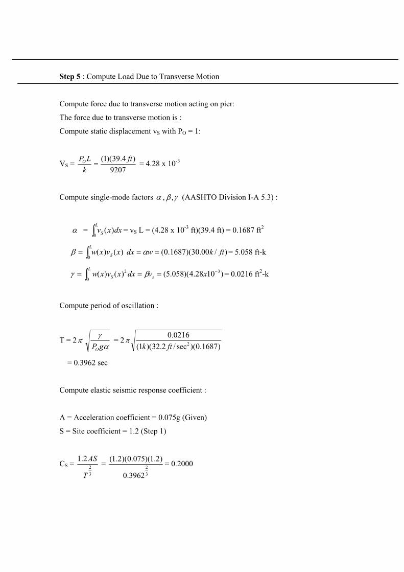
Step 5 : Compute Load Due to Transverse Motion

Compute force due to transverse motion acting on pier:

The force due to transverse motion is :

Compute static displacement vS with PO = 1:

VS = 9207

)4.39)(1( ft

k

LPO = 4.28 x 10-3

Compute single-mode factors , , (AASHTO Division I-A 5.3) :

= = vL

S dxxv0

)( S L = (4.28 x 10-3 ft)(39.4 ft) = 0.1687 ft2

= 5.058 ft-k )/00.30)(1687.0()()(0

ftkwdxxvxwL

S

= 0.0216 ft)1028.4)(058.5()()( 3

0

2 xvdxxvxw s

L

S2-k

Compute period of oscillation :

T = 2gPO

= 2)1687.0)(sec/2.32)(1(

0216.02ftk

= 0.3962 sec

Compute elastic seismic response coefficient :

A = Acceleration coefficient = 0.075g (Given)

S = Site coefficient = 1.2 (Step 1)

CS = 3

2

2.1

T

AS =

3

2

3962.0

)2.1)(075.0)(2.1(= 0.2000

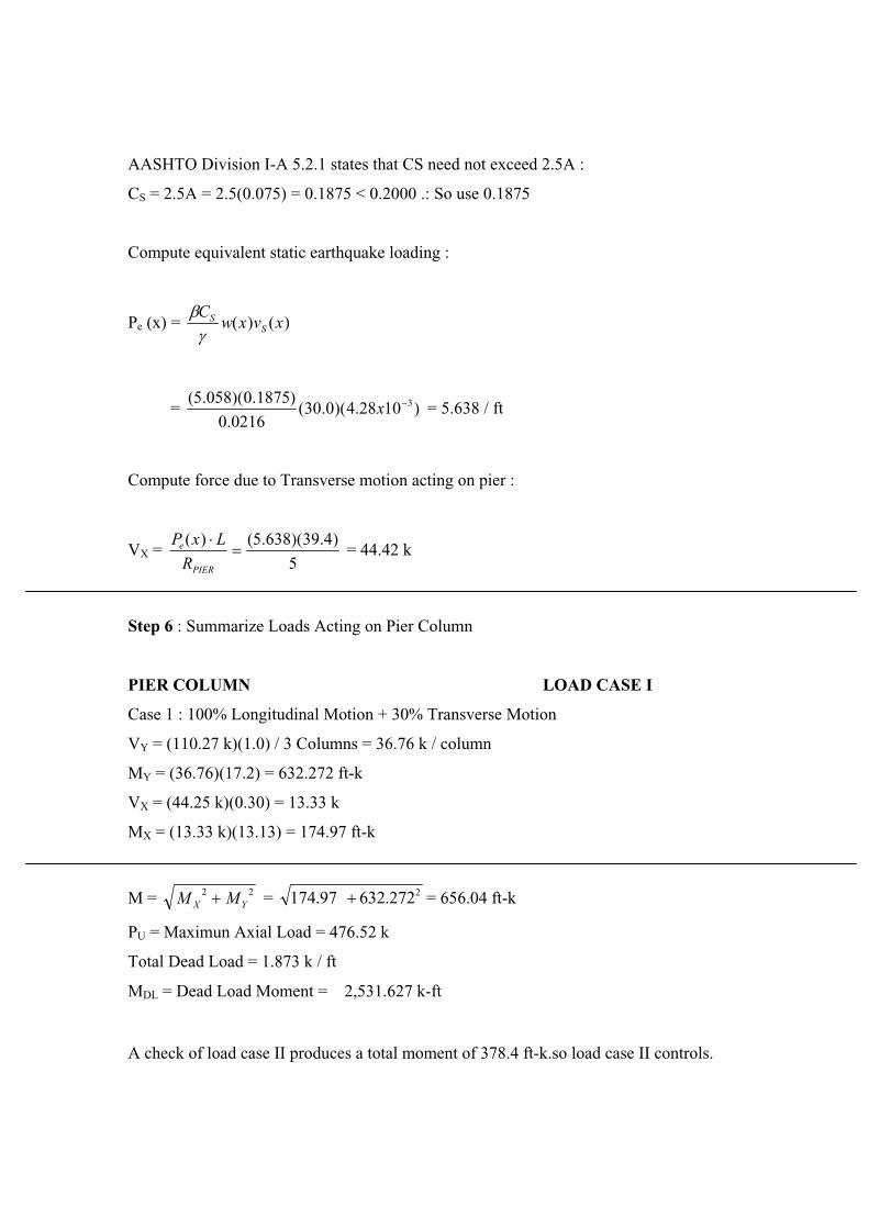
AASHTO Division I-A 5.2.1 states that CS need not exceed 2.5A :

CS = 2.5A = 2.5(0.075) = 0.1875 < 0.2000 .: So use 0.1875

Compute equivalent static earthquake loading :

Pe (x) = )()( xvxwC

SS

= )1028.4)(0.30(0216.0

)1875.0)(058.5( 3x = 5.638 / ft

Compute force due to Transverse motion acting on pier :

VX = 5

)4.39)(638.5()(

PIER

e

R

LxP = 44.42 k

Step 6 : Summarize Loads Acting on Pier Column

PIER COLUMN LOAD CASE I

Case 1 : 100% Longitudinal Motion + 30% Transverse Motion

VY = (110.27 k)(1.0) / 3 Columns = 36.76 k / column

MY = (36.76)(17.2) = 632.272 ft-k

VX = (44.25 k)(0.30) = 13.33 k

MX = (13.33 k)(13.13) = 174.97 ft-k

M = 22YX MM = 2272.63297.174 = 656.04 ft-k

PU = Maximun Axial Load = 476.52 k

Total Dead Load = 1.873 k / ft

MDL = Dead Load Moment = 2,531.627 k-ft

A check of load case II produces a total moment of 378.4 ft-k.so load case II controls.

Step 7 : Checks for Effects of Slenderness

Unsupported Column Length (AASHTO 8.16.5.2.1) :

LU = 26 ft

Radius of Gyration (AASHTO 8.16.5.2.2): k=1.0 k=2.0

r = qlS = (0.25 for circular member)(4ft) = 1.0 ft

Effective length factor :

The effective length factor used will vary

depending on the earthquake motion and

the corresponding orientation of the pier.

Keep in the mind the following :

Transverse Earthquake Motion

Longitudinal Pier Direction

Longitudinal Earthquake Motion Transverse Motion Longitudinal Motion

Transverse Pier Direction

Pier direction are in reference to bridge centerline.

Check Slenderness Ratio Limit (AASHTO 8.16.5.2.5) :

0.1

)26)(0.1( ft

r

Lk U = 26 > 22 : Column is SLENDER for Transverse Motion.

0.1

)26)(0.2( ft

r

Lk U = 52 > 22 : Column Is SLENDER for Longitudinal Motion.

Step 8 : Compute Moment Magnification Factor

pproximation Effects of Creep (AASHTO 8.16.5.2.7 ) : A

04.656

627.2531

tquakeMomenTotalEarth

oadTotalDeadLd

= 3.86

t of Inertia of Gross Concrete Section :

g =

Momen

I64

)]/12()95.2[(

64

44 ftinD=77.09 x 10 3 in4

pute Flexural Rigidity (Equation 4.28) :

EI =

Com

86.315.2

)1009.77(000,300,3

15.2

3xpsiIE gC

= 1.047 x 1011 Ib in2

ompute Factor Relating Actual Moment Diagram to Equivalent :

ompute Critical Buckling Load (Equation 4.26 ):

C =

C

CM = 1.0

C

2

112

2

2

))/12)(26)(0.2((

)10047.1(

)( ftinft

x

kL

EI

U

P = 2653,855.35 k

Compute Moment Magnification Factor (Service Load Approach):

C

U

m

P

PC

50.21

=

)35.855,2653(0.1

)52.476)(50.2(1

0.1

k

k = 1.00045

tep 9 : Determine Required Reinforcing Steel : S

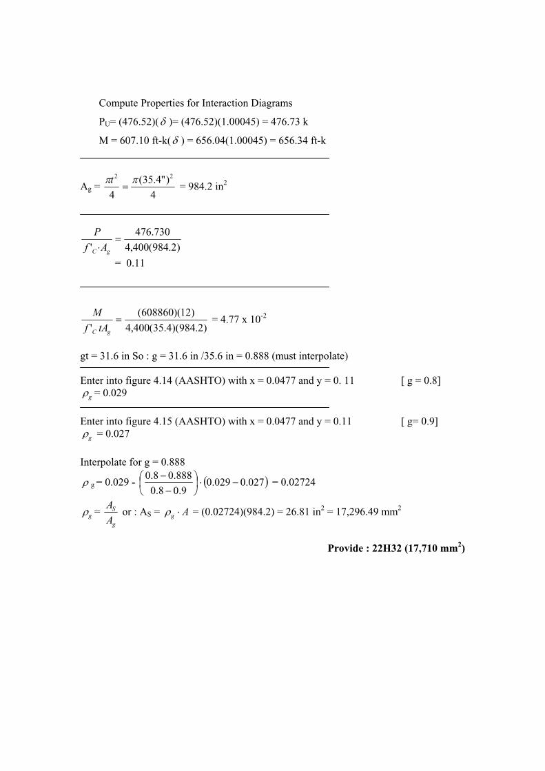
Compute Properties for Interaction Diagrams

PU= (476.52)( )= (476.52)(1.00045) = 476.73 k

kM = 607.10 ft- ( ) = 656.04(1.00045) = 656.34 ft-k

Ag = 4

)"4.35( 22t = 984.2 in2

4

)2.984(400,4

730.476

' gC Af

P

= 0.11

)2.984)(4.35(400,4

)12)(608860(M -2

' gC tAf = 4.77 x 10

t = 31.6 in So : g = 31.6 in /35.6 in = 0.888 (must interpolate)

[ g = 0.8]

g

nter into figure 4.14 (AASHTO) with x = 0.0477 and y = 0. 11Eg = 0.029

Enter into figure 4.15 (AASHTO) with x = 0.0477 and y = 0.11 [ g= 0.9] g = 0.027

terpolate for g = 0.888In

027.0029.09.08.0

888.08.0 = 0.02724 g = 0.029 -

g =g

SAAgA

or : AS = = (0.02724)(984.2) = 26.81 in2 = 17,296.49 mm2

Provide : 22H32 (17,710 mm2)

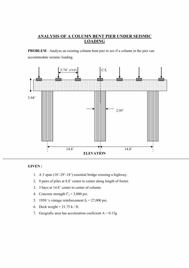
ANALYSIS OF A COLUMN BENT PIER UNDER SEISMICLOADING

PROBLEM : Analyze an existing column bent pier to see if a column in the pier can

accommodate seismic loading.

5.74’ (TYP) C/L

3.94’

2.95’

14.8’ 14.8’ELEVATION

GIVEN :

1. A 3 span (18’-29’-18’) essential bridge crossing a highway.

2. 9 pairs of piles at 8.8’ center to center along length of footer.

3. 3 bays at 14.8’ center to center of column.

4. Concrete strength f’c = 3,000 psi.

5. 1950 ‘s vintage reinforcement fS = 27,000 psi.

6. Deck weight = 21.75 k / ft.

7. Geografic area has acceleration coeficient A = 0.15g

Step 1 : Determine Type of Seismic Analysis and Other Criteria

For an “essential bridge” by AASHTO 3.3 I-A we have:

IC = Importance Classification = I

With an importance classification of “I” by AASHTO 3.4 I-A for :

0.09 < A < 0.19 and IC = I

SPC = Seismic Performance Category = B

The bridge has an unchanging cross section,with similar supports, and a uniform mass

and stiffness,so it is considered to be :

Regular (By AASHTO 4.2 I-A)

For a Regular Bridge, SPC = B, and 2 or more spans, use:

Method 1 = Single-Mode Spectral Analysis (By AASHTO 4.2 I-A)

For stiff clay,by AASHTO 3.5 I-A:

Soil Profile Type II: S = Site Coefficient = 1.2

Response Modification Factor (AASHTO 3.6 I-A)

Multiple Column Bent: R = 5 (Treat as a wall-type pier)

Pier footing: R = One-Half R for Multiple Column Bent

= R/2 = 5/2 = 2.25 (AASHTO 4.7.2 I-A)

Combination of Seismic Forces (AASHTO 4.4 I-A):

Case I : [100% Longitudinal Motion] + [30% Tranverse Motion]

Case II : [30% Longitudinal Motion] + [100 % Tranverse Motion}

Load Grouping (AASHTO 4.7.1 I-A) :

1.0(DL + Buoyancy + Stream Flow + Earth Pressure + Earthquake)

(N/A) (N/A)

Step 2 : Compute Stiffness of the Pier

h = 24’

Longitudinal Earthquake Transverse Earthquake Motion Motion

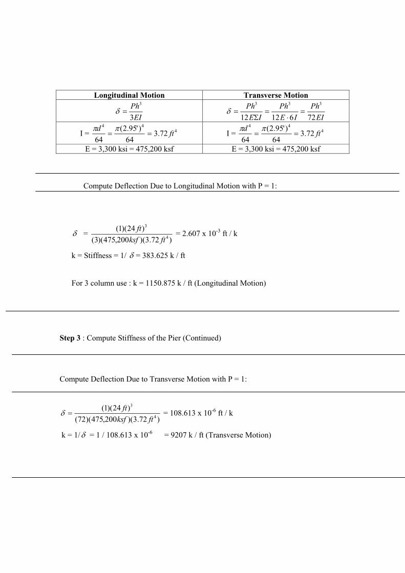
Longitudinal Motion Transverse Motion

EI

Ph

3

3

EI

Ph

IE

Ph

IE

Ph

7261212

333

I = 444

72.364

)'95.2(

64ft

dI = 4

44

72.364

)'95.2(

64ft

d

E = 3,300 ksi = 475,200 ksf E = 3,300 ksi = 475,200 ksf

Compute Deflection Due to Longitudinal Motion with P = 1:

= )72.3)(200,475)(3(

)24)(1(4

3

ftksf

ft = 2.607 x 10-3 ft / k

k = Stiffness = 1/ = 383.625 k / ft

For 3 column use : k = 1150.875 k / ft (Longitudinal Motion)

Step 3 : Compute Stiffness of the Pier (Continued)

Compute Deflection Due to Transverse Motion with P = 1:

)72.3)(200,475)(72(

)24)(1(4

3

ftksf

ft = 108.613 x 10-6 ft / k

k = 1/ = 1 / 108.613 x 10-6 = 9207 k / ft (Transverse Motion)

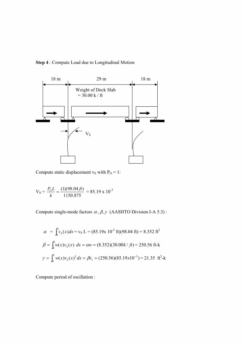
Step 4 : Compute Load due to Longitudinal Motion

18 m 29 m 18 m

Weight of Deck Slab = 30.00 k / ft

VS

Compute static displacement vS with PO = 1:

VS = 875.1150

)04.98)(1( ft

k

LPO = 85.19 x 10-3

Compute single-mode factors , , (AASHTO Division I-A 5.3) :

= = vL

S dxxv0

)( S L = (85.19x 10-3 ft)(98.04 ft) = 8.352 ft2

= 250.56 ft-k )/00.30)(352.8()()(0

ftkwdxxvxwL

S

= 21.35 ft)1019.85)(56.250()()( 3

0

2 xvdxxvxw s

L

S2-k

Compute period of oscillation :

T = 2gPO

= 2)352.8)(sec/2.32)(1(

35.212ftk

= 1.770 sec

Compute elastic seismic response coefficient :

A = Acceleration coefficient = 0.15g (Given)

S = Site coefficient = 1.2 (Step 1)

CS = 3

2

2.1

T

AS =

3

2

770.1

)2.1)(15.0)(2.1(= 0.1476

AASHTO Division I-A 5.2.1 states that CS need not exceed 2.5A :

CS = 2.5A = 2.5(0.15) = 0.375 > 0.1476 .: So use 0.1476

Compute equivalent static earthquake loading :

Pe (x) = )()( xvxwC

SS

= )1019.85)(0.30(35.21

)1476.0)(56.250( 3x = 4.4270 k / ft

Compute force due to longitudinal motion acting on pier :

VY = 5

)04.98)(4270.4()(

PIER

e

R

LxP = 86.80 k

Step 5 : Compute Load Due to Transverse Motion

Compute force due to transverse motion acting on pier:

The force due to transverse motion is :

Compute static displacement vS with PO = 1:

VS = 9207

)4.39)(1( ft

k

LPO = 4.28 x 10-3

Compute single-mode factors , , (AASHTO Division I-A 5.3) :

= = vL

S dxxv0

)( S L = (4.28 x 10-3 ft)(39.4 ft) = 0.1687 ft2

= 5.058 ft-k )/00.30)(1687.0()()(0

ftkwdxxvxwL

S

= 0.0216 ft)1028.4)(058.5()()( 3

0

2 xvdxxvxw s

L

S2-k

Compute period of oscillation :

T = 2gPO

= 2)1687.0)(sec/2.32)(1(

0216.02ftk

= 0.3962 sec

Compute elastic seismic response coefficient :

A = Acceleration coefficient = 0.15g (Given)

S = Site coefficient = 1.2 (Step 1)

CS = 3

2

2.1

T

AS =

3

2

3962.0

)2.1)(15.0)(2.1(= 0.4004

AASHTO Division I-A 5.2.1 states that CS need not exceed 2.5A :

CS = 2.5A = 2.5(0.15) = 0.375 < 0.4004 .: So use 0.375

Compute equivalent static earthquake loading :

Pe (x) = )()( xvxwC

SS

= )1028.4)(0.30(0216.0

)375.0)(058.5( 3x = 11.275k / ft

Compute force due to Transverse motion acting on pier :

VX = 5

)4.39)(275.11()(

PIER

e

R

LxP = 88.85 k

Step 6 : Summarize Loads Acting on Pier Column

PIER COLUMN LOAD CASE I

Case 1 : 100% Longitudinal Motion + 30% Transverse Motion

VY = (86.80 k)(1.0) / 3 Columns = 28.933 k / column

MY = (28.933)(17.2) = 497.65 ft-k

VX = (88.25 k)(0.30) = 26.48 k

MX = (26.48 k)(13.13) = 347.77 ft-k

M = 22YX MM = 265.49777.347 = 607.12 ft-k

PU = Maximun Axial Load = 476.52 k

Total Dead Load = 1.873 k / ft

MDL = Dead Load Moment = 2,531.627 k-ft

A check of load case II produces a total moment of 378.4 ft-k.so load case II controls.

Step 7 : Checks for Effects of Slenderness

Unsupported Column Length (AASHTO 8.16.5.2.1) :

LU = 26 ft

Radius of Gyration (AASHTO 8.16.5.2.2): k=1.0 k=2.0

r = qlS = (0.25 for circular member)(4ft) = 1.0 ft

Effective length factor :

The effective length factor used will vary

depending on the earthquake motion and

the corresponding orientation of the pier.

Keep in the mind the following :

Transverse Earthquake Motion

Longitudinal Pier Direction

Longitudinal Earthquake Motion Transverse Motion Longitudinal Motion

Transverse Pier Direction

Pier direction are in reference to bridge centerline.

Check Slenderness Ratio Limit (AASHTO 8.16.5.2.5) :

0.1

)26)(0.1( ft

r

Lk U = 26 > 22 : Column is SLENDER for Transverse Motion.

0.1

)26)(0.2( ft

r

Lk U = 52 > 22 : Column Is SLENDER for Longitudinal Motion.

Step 8 : Compute Moment Magnification Factor

pproximation Effects of Creep (AASHTO 8.16.5.2.7 ) : A

12.607

627.2531

tquakeMomenTotalEarth

oadTotalDeadLd

= 4.17

t of Inertia of Gross Concrete Section :

g =

Momen

I64

)]/12()95.2[(

64

44 ftinD=77.09 x 10 3 in4

pute Flexural Rigidity (Equation 4.28) :

EI =

Com

17.415.2

)1009.77(000,300,3

15.2

3xpsiIE gC

= 1.968 x 1010 Ib in2

ompute Factor Relating Actual Moment Diagram to Equivalent :

ompute Critical Buckling Load (Equation 4.26 ):

C =

C

CM = 1.0

C

2

102

2

2

))/12)(26)(0.2((

)10968.1(

)( ftinft

x

kL

EI

U

P = 498,834 k

Compute Moment Magnification Factor (Service Load Approach):

C

U

m

P

PC

50.21

=

)834,498(0.1

)52.476)(50.2(1

0.1

k

k = 1.00239

tep 9 : Determine Required Reinforcing Steel : S

Compute Properties for Interaction Diagrams

PU= (476.52)( )= (476.52)(1.00239) = 477.66 k

kM = 607.10 ft- ( ) = 607.10(1.0029) = 608.86 ft-k

Ag = 4

)"4.35( 22t = 984.2 in2

4

)2.984(400,4

477660

' gC Af

P

= 0.11

)2.984)(4.35(400,4

)12)(608860(M -2

' gC tAf = 4.77 x 10

t = 31.6 in So : g = 31.6 in /35.6 in = 0.888 (must interpolate)

[ g = 0.8]

g

nter into figure 4.14 (AASHTO) with x = 0.0477 and y = 0. 11Eg = 0.029

Enter into figure 4.15 (AASHTO) with x = 0.0477 and y = 0.11 [ g= 0.9] g = 0.027

terpolate for g = 0.888In

027.0029.09.08.0

888.08.0 = 0.02724 g = 0.029 -

g =g

SAAgA

or : AS = = (0.03784)(984.2) = 26.81 in2 = 17,296.49 mm2

Provide : 22H32 (17,710 mm2)

DESIGN OF A STUB ABUTMENT WITH SEISMIC CODE

PROBLEM : Design a stub abutment to accommodate given reactions from a composite

steel superstructure. 2.62’

V

13.73’

2.62’

4.43’

6.56’

Given :

1. A 3 span ( 59’-98’-59’) essential bridge crossing a highway.

2. 2.0 ‘ diameter concrete piles – 50 ft long.Capacity = 140 ton

3. 9 pairs of piles at 9’ center to center along length of footer.

4. Concrete strength f ‘C = 7,300psi = C50

5. Grade 50 reinforcement f ‘S = 27,000 psi =

6. Total reaction from all stringer R = 387 k.

7. Deck weight = 21.74 k/ft

8. Geografic area has acceleration coefficient : A = 0.075.

9. Soil test indicate stiff clay with angle of friction : 30

Step 1 : Determine Type of Seismic Analysis and Other Criteria

For an “essential bridge” by AASHTO 3.3 I-A we have :

IC = Importance Classification = I

With an importance classification of “I” by AASHTO 3.4 I-A for :

0.09<A<0.19 and IC = II

SPC = Seismic Performance Category = B

The bridge has an unchanging cross section,with similar supports,and a uniform mass and

stiffness,so it is considered to be :

Regular (By AASHTO 4.2 I-A)

For a Regular Bridge,SPC = B,and or more spans,use :

Method 1 = Single Mode Spectral Analysis (BY AASHTO 4.2 I-A)

For stiff clay, by AASHTO 3.5 I-A:

Soil Profile Type II:S = Site Coefficient = 1.2

Response Modification Factor (AASHTO 3.6 I-A)

Abutment Stem : R = 2 (Treat as a wall-type pier)

Abutment Footing : R = One – half R for abutment stem.

= R/2 = 2/2 = 1 (AASHTO 4.7.2 I-A)

Combination of Seismic Performance (AASHTO 4.4 I-A) :

Case I : 100 % Longitudinal Motion + 30% Tranverse Motion

Case II : 30% Longitudinal Motion + 100 % Tranverse Motion

Load Grouping (AASHTO 4.7.1 I-A):

1.0(DL = Buoyancy + Stream Flow + Earth Pressure + Earthquake

Step 2 : Compute Seismic Active Earth Pressure

Using the Monokobe- Okabe Equation (AASHTO C6.3.2 I-A) :

PAE = AEV KKH )1(21 2

Where the seismic active pressure coefficient is defined as :

KAE = )cos(coscos

)(cos2

2

Where :

= Angle of Friction of soil = 30 ˚ (Given) = Angle of friction between soil and abutment = 0 (Smooth)

I = Backfill slope angle = 0 (Level Backfill) = Slope of soil face = 0 (Vertical Rear Face of Stem)

and where :

= ATANV

h

k

k

1 kh = Horizontal acceleration Coefficient

= ATAN045.01

1125.0 = 1.5A = (1.5)(0.075) = 0.1125

kV = Vertical Acceleration Coefficient

= 6.72˚ 7 ˚ 0.3kh < kV < 0.5kh

(0.3)(0.1125) < kV < (0.5)(0.1125)

0.03375 < kV < 0.05625 So use :

kV = 0.045

Check horizontal acceleration coefficient (AASHTO C6.3.2 I-A):

Kh < (1-kV)tan( -I) so : 0.045 < (1-0.045)(tan(30-0)) < 0.5514

= 2

)cos()cos(sin()sin(1

i

i

= 2

)0cos()700cos()730sin()030sin(1

= 1.1969

Recall that the seismic active pressure coefficient is defined as :

KAE =)cos(coscos

)(cos2

2

= )700cos()0(cos)7cos()1969.1(

)0730(cos2

2

= 0.7183

Also recall that the Monokobe- Okabe Equation is defined as :

PAE = AEV kkH )1(21 2

So for the whole wall :

)955.0()14)(/120(21 23ftIbPAE = = 11,230.8 Ib / ft

Step 3 : Compute Static Active Earth Pressure

The static active earth pressure coefficient is defined as :

KA = )cos(cos

)(cos2

2

=

Where :

2

)cos()cos()sin()sin(1

2

)0cos()0cos()30sin()30sin(1

i

i =

= 2.25

KA = )cos(cos

)(cos2

2

=)00cos()0(cos)25.2(

)030(cos2

2

= 0.3333

o the static active earth pressure is defined as : S

PA = AKH 212

o for the whole wall : S

PA = )3333.0()14)(/120(1 3ftIb2

2 = 3916.08 Ib/ft

tep 4 : Compute Equivalent PressureS

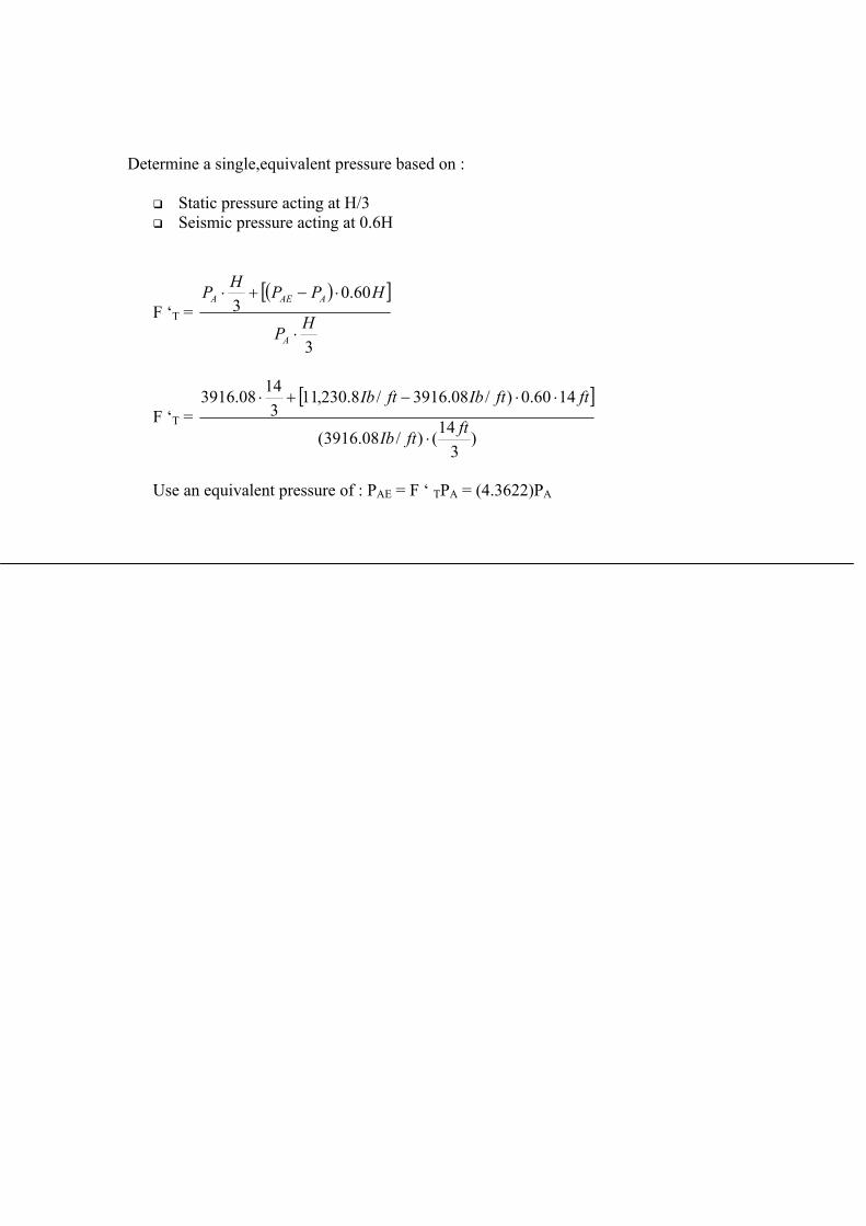
Determine a single,equivalent pressure based on :

Seismic pressure acting at 0.6H

‘T =

Static pressure acting at H/3

F

3

60.03

HP

HPPH

P

A

AAEA

)3

14()/08.3916(

1460.0)/08.3916/8.230,113

1408.3916

ftftIb

ftftIbftIbF ‘T =

Use an equivalent pressure of : PAE = F ‘ TPA = (4.3622)PA

Step 5 : Compute Abutment Loads

calculation in step 1

DL

Y

PAE

R3

2

ompute all Wi loads from abutment and soil:

NOTE :

Wi and DL there is a

For all dimensions refer to figure on

For all loads

corresponding load kVWi and kVDL

acting upward (kV > 0) or

downward (kV <0)

All Wi loads are based on a per pile

pair basis.Recall that the distance

between piles along the length of

footing was given as 9’ = 9 ft

Use the following unit weights :3CONCRETE = 145 Ib/ft

3SOIL = 120 Ib/ft

V

h W1K

h W2K

W3

R

C

W2

hW3K

Wi = (Height)(Width)(Pile Distance)(Weight)

1 = (5.66ft)(2.62 ft)(9.0 ft)(0.150 k / ft ) = 20.0 k 3

ecall that the dead load from the superstructure was given as :

tep 6 : Compute Active Earth Pressure for Stem and Wall

H = 14 ‘ (WHOLE WALL PA

1’ Stem

WALL 4

sing Rankie equation for :

3W

W2 = (2.62ft)(5.09ft)(9.0 ft)(0.150 k/ft ) = 18.0 k

W3 = (4.43 ft)(8.2 ft)(9.0 ft)(0.150 k/ft3) = 49.0 k

W4 = (8.40 ft)(1.312)(9.0ft)(0.120 k/ft3) = 11.90 k

R

DL = 387 k / 9 pairs of piles = 43.0 k / pair

S

H = 9.30’ (STEM)

)

3.PA

.7 ‘

U

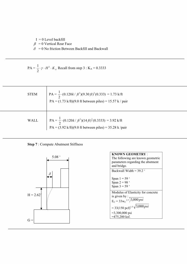
I = 0 Level backfill = 0 Vertical Rear Face = 0 No friction Between Backfill and Backwall

PA = AKH 2

21 Recall from step 3 : KA = 0.3333

TEM PA = S )333.0()30.9)(/120.0(21 23 ftftk = 1.73 k/ft

(1.73 k/ft)(9.0 ft between piles) = ir

ALL PA =

PA = 15.57 k / pa

W )3333.0()14)(/120.0(21 23 ftftk = 3.92 k/ft

(3.92 k/ft)(9.0 ft between piles) ir

tep 7 : Compute Abutment Stiffness

5.08 ‘

PA = = 35.28 k /pa

S

H = 2.62

=

KNOWN GEOMETRY : The following are known geometric

tment

’

G 0.4E = 190080 ksf

parameters regarding the abuand bridge.Backwall Width = 39.2 ‘

Span 1 = 59 ‘pan 2 = 98 ‘S

Span 3 = 59 ‘

Modulus of Elasticity for concreteis given by : EC = 33wC

1.5 psi000,3

= 33(150 pcf)1.5 psi000,3

=3,300,000 psi=475,200 ksf.

Compute Deflection Considering Effects of Shear with P = 1 :

=AG

Ph

EI

Ph 2.13

or : Ebd

hhh

EbdEAEI

h 2.1122.1 33

3 4.034.03 3

Where : The equation above can be rewritten as :

= 2.62’H

bEdd

34 hh3

D = 5.08’ )'2.39)(200,475(

)52.0(3)52.0(4 3

B = 39.2’

= 0.000000113 ft/k

52.0'08.5'62.2H k = stiffness = 1/

D = 8,776,648.7 k/ft

tep 8 : Compute Earthquake Load on Abutment

59 ‘ 98 ‘ 59 ‘

vS

ompute static displacement vS with PO = 1 :

S

w = weight of deck = 21.74 k/ft

C

VS = k

LPO = ftk

ft)0.98)(1( = 11.17 x 10 /7.8776648

Compute single-mode factors

-6

,, (AASHTO Division I-A 5.3) = vSL = (11.17 x 10 –6)(98) = 1.09x 10 –3 ft2dxxvS

L )(0

= )(0

= 23.80 x 10 ft k vxw S wdxx)( = (1.09 x 10 ft )(21.74 k/ft)

–3

L –3 2

= = (23.80 x 10-3)(11.17 x 10-6)= 265.82x 10 ft k

Co lation :

SSL vdxxvxw 20 )()(

-9 2

mpute period of oscil

)1009.1)(sec/2.32)(1(1082.262T = 2 5

32

298

xftk

kftx

gPO

3 sec

ompute Elastic Seismic Response Coefficient :

= Site coefficient = 1.2 (step 1)

= 0.017

C

A = Acceleration Coefficient = 0.075 (Given)

S

CS = 32

2.1

T

AS = 32

)2.1)(075.0(2.1 =0173.0

1.61

AASHTO Division I-A 5.2.1 states that CS need not exceed 2.5A :

CS = 2.5A = (2.5)(0.075) = 0.1875 < 1.61 Use : CS = 0.1875

Compute equivalent static earthquake loading :

Pe(x) = )()( xvxw SSC

= 9

3

1082.265)1875.01080.23(

x

kxftx x (21.74 k /ft)(11.17x 10-6)

= 4.0785 k / ft

acting on abutment :

Y

Compute force

V = 0.2

)98)(/0785.4()( ftftkLxpe

RSTEM

= 199.85 k

tep 9 : Compute Shears and Moments

VY 6’

PAE.6’

3.1’

Previously Determined Values

NOTE :

For all loads Wi and DL there is a

ding load kVWi and kVDL

rd

S

8”12 ”

DL

5

1.31’

correspon

acting upward (kV > 0) or downwa

(kV < 0).

KhW2

W2

A

0.1125

W1 = 20.0 k ,kV = 0.045

Step 6

AE = 4.3622 PA = 4.3622 (15.57 k /Pair) = 67.92 k/pair step 4

step 8

Y = (199.85 k) / 9 pairs of piles

kV) kV > 0

+ 20.0 k + 18.0 k )(1-0.045) -77.36 k

V < 0

= - (43.0 k + 20.0 k + 18.0 k)(1 + 0.045) -84.65 k

= (0.1125)(43.0 k) + (0.1125)(20.0 k) + (0.1125)(18) k + 22.21 k + 67.92

F =

DL = 43.0 k , W2 = 18 k , kh =

Active pressure acting on stem :

PA = 15.57 k / pair

P

Superstructure loads acting on a pair of piles :

VY = 199.85 k

V

= 22.21 k

V= 0: -(DL + W1 + W2)(1-

= - (43.0 k

V= 0: -(DL + W1 + W2 )(1+kV) k

H = 0: khDL + khW1 + khW2 +VY + PAE

99.24 k

Axial Force:

ApilesBetDist. ween

VMAX = ft

k

0.965.84 = FA = 9.41k/ft

Force :

V =

Shear

pilesBetwDist. een

H = ft

k

0.924.99 = V = 11.03 k / ft

= 0: h

5.6VY+ 1.0DL (1+kV) + 3.1PAE + 6khW1 + 2W2kh – 0.67W1(1+ kV)

MA [k < 0][kV>0]

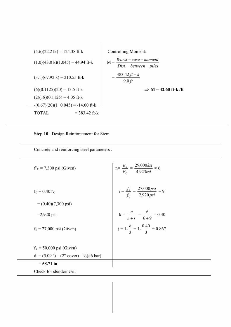
.0)(43.0 k)(1.045) = 44.94 ft-k M =

(5.6)(22.21k) = 124.38 ft-k Controlling Moment:

(1piles

momentcaseWorst

betweenDist.

(3.1)(67.92 k) = 210.55 ft-k = ft

kft

0.942.383

(6)(0.1125)(20) = 13.5 ft-k M = 42.60 ft-k /ft

(2)(18)(0.1125) = 4.05 ft-k

0 ft-k

.42 ft-k

tep 10 : Design Reinforcement for Stem

n=

-(0.67)(20)(1+0.045) = -14.0

TOTAL = 383

S

Concrete and reinforcing steel parameters :

f’C = 7,300 psi (Given)C

S

E

E = ksi

ksi

923,4000,29 6

fC = 0.40f’C r = C

S

f

f = psi

psi

920,2000,27 = 9

=2,920 psi k =

= (0.40)(7,300 psi)

rn

n = 96

6 = 0.40

i (GfS = 27,000 ps iven) j = 1-3k

340.0= 1- = 0.867

= (5.09 ‘) – (2” cover) – ½(#6 bar)

fY = 50,000 psi (Given)

d

= 58.71 in

Check for slenderness :

LU = Unsupported length By AASHTO 8.16.5.2.5 effect of

= 2.62 ft slenderness may be ignored if the

r = radius of gyration

slenderness ratio is less than 22

r

Lk U = 0.1

)62.2)(0.2( = 5.24 < 22

= (0.30)(3.333) = 1.0 Therefore member is not slender

k= effective length factor

Des n ed main reinforcement :

= 2.0

ig requir

AS = jdf

M = )71.58)(867.0(27

)/12)(60.42( ftin

S inksi

all = 791.998 mm2/ meterfor right and left moment, 791.998 x 7.0 meter = 5,543.99 mm2

o : Use , 7H32 (5632 mm2)

= 0.372 in2 / ft of w

S

Compute design moment strength (AASHTO 8.16.3.2) :

NM = 2

dfA YS

a

a = )12)(/300,7(85.0)/000,50)(34.

2

22

ininIb

inIbinch = 0.2283 in 0(bf

fA YS

C'85.0So : a =

nM = 0.9[(0.34 in)(50,000 Ib/in2)(58.71 in - 2

228MU = .0

= 896,516.51 in.b = 74.71 ft-k > 35.56 ft-k

3 )]

Design for shear – friction (AASHTO 8.15.5.4) :

Sf

VAvf = Required Shear – Friction reinforcement =

V = 11.03 k/ft step 9

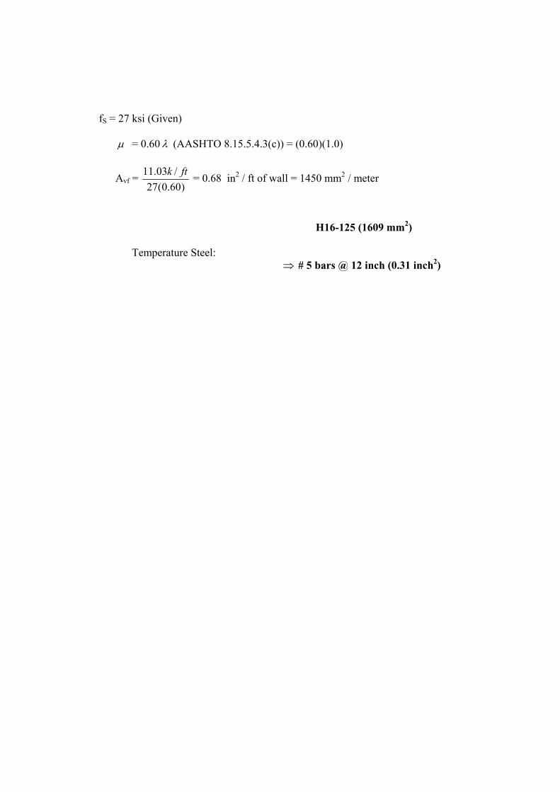
fS = 27 ksi (Given)

= 0.60 (AASHTO 8.15.5.4.3(c)) = (0.60)(1.0)

Avf = )60(27

= 0.68 in / ft of wall = 1450 mm /.0

/03.11 ftk meter

H16-125 (1609 mm2)

Temperature Steel: ch2)

2 2

# 5 bars @ 12 inch (0.31 in

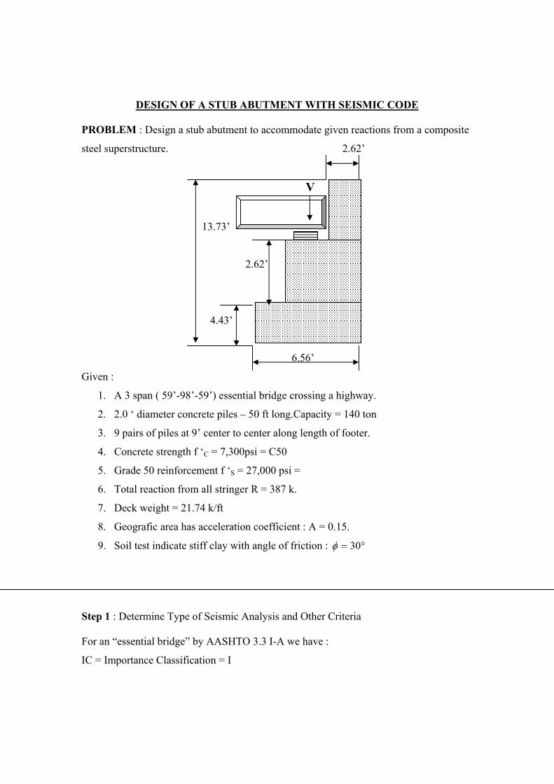
DESIGN OF A STUB ABUTMENT WITH SEISMIC CODE

PROBLEM : Design a stub abutment to accommodate given reactions from a composite

steel superstructure. 2.62’

V

13.73’

2.62’

4.43’

6.56’

Given :

1. A 3 span ( 59’-98’-59’) essential bridge crossing a highway.

2. 2.0 ‘ diameter concrete piles – 50 ft long.Capacity = 140 ton

3. 9 pairs of piles at 9’ center to center along length of footer.

4. Concrete strength f ‘C = 7,300psi = C50

5. Grade 50 reinforcement f ‘S = 27,000 psi =

6. Total reaction from all stringer R = 387 k.

7. Deck weight = 21.74 k/ft

8. Geografic area has acceleration coefficient : A = 0.15.

9. Soil test indicate stiff clay with angle of friction : 30

Step 1 : Determine Type of Seismic Analysis and Other Criteria

For an “essential bridge” by AASHTO 3.3 I-A we have :

IC = Importance Classification = I

With an importance classification of “I” by AASHTO 3.4 I-A for :

0.09<A<0.19 and IC = II

SPC = Seismic Performance Category = B

The bridge has an unchanging cross section,with similar supports,and a uniform mass and

stiffness,so it is considered to be :

Regular (By AASHTO 4.2 I-A)

For a Regular Bridge,SPC = B,and or more spans,use :

Method 1 = Single Mode Spectral Analysis (BY AASHTO 4.2 I-A)

For stiff clay, by AASHTO 3.5 I-A:

Soil Profile Type II:S = Site Coefficient = 1.2

Response Modification Factor (AASHTO 3.6 I-A)

Abutment Stem : R = 2 (Treat as a wall-type pier)

Abutment Footing : R = One – half R for abutment stem.

= R/2 = 2/2 = 1 (AASHTO 4.7.2 I-A)

Combination of Seismic Performance (AASHTO 4.4 I-A) :

Case I : 100 % Longitudinal Motion + 30% Tranverse Motion

Case II : 30% Longitudinal Motion + 100 % Tranverse Motion

Load Grouping (AASHTO 4.7.1 I-A):

1.0(DL = Buoyancy + Stream Flow + Earth Pressure + Earthquake

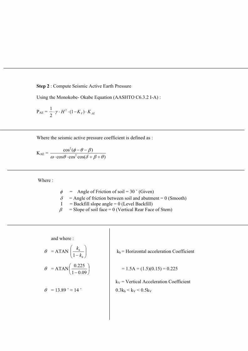
Step 2 : Compute Seismic Active Earth Pressure

Using the Monokobe- Okabe Equation (AASHTO C6.3.2 I-A) :

PAE = AEV KKH )1(21 2

Where the seismic active pressure coefficient is defined as :

KAE = )cos(coscos

)(cos2

2

Where :

= Angle of Friction of soil = 30 ˚ (Given) = Angle of friction between soil and abutment = 0 (Smooth)

I = Backfill slope angle = 0 (Level Backfill) = Slope of soil face = 0 (Vertical Rear Face of Stem)

and where :

= ATANh

h

k

k

1 kh = Horizontal acceleration Coefficient

= ATAN09.01

225.0 = 1.5A = (1.5)(0.15) = 0.225

kV = Vertical Acceleration Coefficient

= 13.89 ˚ 14 ˚ 0.3kh < kV < 0.5kV

(0.3)(0.225) < kV < (0.5)(0.225)

0.0675 < kV < 0.1125 So use :

kV = 0.09

Check horizontal acceleration coefficient (AASHTO C6.3.2 I-A):

Kh < (1-kV)tan( -I) so : 0.225 < (1-0.09)(tan(30-0)) < 0.525

= 2

)cos()cos(sin()sin(1

i

i

= 2

)0cos()1400cos()1430sin()030sin(1

= 1.896

Recall that the seismic active pressure coefficient is defined as :

KAE =)cos(coscos

)(cos2

2

= )1800cos()0(cos)18cos()896.1(

)01430(cos2

2

= 0.5388

Also recall that the Monokobe- Okabe Equation is defined as :

PAE = AEV kkH )1(21 2

So for the whole wall :

)91.0()14)(/120(21 23ftIbPAE = = 10,701.6Ib / ft

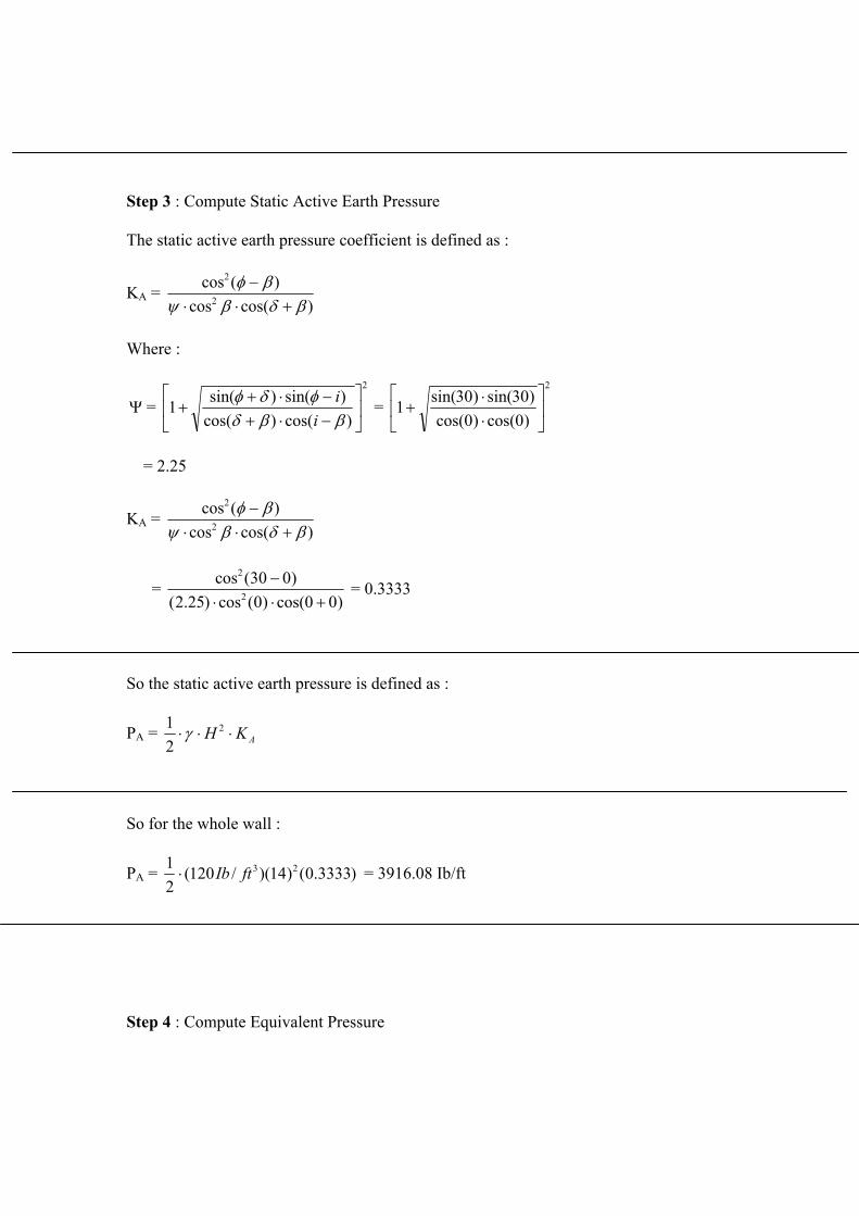
Step 3 : Compute Static Active Earth Pressure

The static active earth pressure coefficient is defined as :

KA = )cos(cos

)(cos2

2

=

Where :

2

)cos()cos()sin()sin(1

2

)0cos()0cos()30sin()30sin(1

i

i =

= 2.25

KA = )cos(cos

)(cos2

2

=)00cos()0(cos)25.2(

)030(cos2

2

= 0.3333

o the static active earth pressure is defined as : S

PA = AKH 212

o for the whole wall : S

PA = )3333.0()14)(/120(1 3ftIb2

2 = 3916.08 Ib/ft

tep 4 : Compute Equivalent PressureS

Determine a single,equivalent pressure based on :

Seismic pressure acting at 0.6H

‘T =

Static pressure acting at H/3

F

3

60.03

HP

HPPH

P

A

AAEA

)3

14()/08.3916(

1460.0)/08.3916/6.107013

1408.3916

ftftIb

ftftIbftIbF ‘T =

Use an equivalent pressure of : PAE = F ‘ TPA = (4.1189)PA

Step 5 : Compute Abutment Loads

calculation in step 1

DL

Y

PAE

R3

2

ompute all Wi loads from abutment and soil:

NOTE :

Wi and DL there is a

For all dimensions refer to figure on

For all loads

corresponding load kVWi and kVDL

acting upward (kV > 0) or

downward (kV <0)

All Wi loads are based on a per pile

pair basis.Recall that the distance

between piles along the length of

footing was given as 9’ = 9 ft

Use the following unit weights :3CONCRETE = 145 Ib/ft

3SOIL = 120 Ib/ft

V

h W1K

h W2K

W3

R

C

W2

hW3K

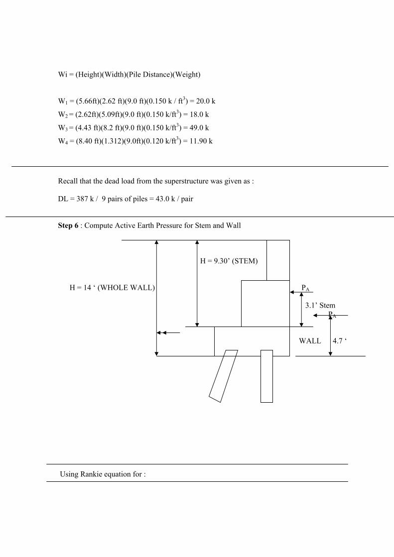
Wi = (Height)(Width)(Pile Distance)(Weight)

1 = (5.66ft)(2.62 ft)(9.0 ft)(0.150 k / ft ) = 20.0 k 3

ecall that the dead load from the superstructure was given as :

tep 6 : Compute Active Earth Pressure for Stem and Wall

H = 14 ‘ (WHOLE WALL PA

1’ Stem

WALL 4

sing Rankie equation for :

3W

W2 = (2.62ft)(5.09ft)(9.0 ft)(0.150 k/ft ) = 18.0 k

W3 = (4.43 ft)(8.2 ft)(9.0 ft)(0.150 k/ft3) = 49.0 k

W4 = (8.40 ft)(1.312)(9.0ft)(0.120 k/ft3) = 11.90 k

R

DL = 387 k / 9 pairs of piles = 43.0 k / pair

S

H = 9.30’ (STEM)

)

3.PA

.7 ‘

U

I = 0 Level backfill = 0 Vertical Rear Face = 0 No friction Between Backfill and Backwall

PA = AKH 2

21 Recall from step 3 : KA = 0.3333

TEM PA = S )333.0()30.9)(/120.0(21 23 ftftk = 1.73 k/ft

(1.73 k/ft)(9.0 ft between piles) = ir

ALL PA =

PA = 15.57 k / pa

W )3333.0()14)(/120.0(21 23 ftftk = 3.92 k/ft

(3.92 k/ft)(9.0 ft between piles) ir

tep 7 : Compute Abutment Stiffness

5.08 ‘

PA = = 35.28 k /pa

S

H = 2.62

=

KNOWN GEOMETRY : The following are known geometric

tment

’

G 0.4E = 190080 ksf

parameters regarding the abuand bridge.Backwall Width = 39.2 ‘

Span 1 = 59 ‘pan 2 = 98 ‘S

Span 3 = 59 ‘

Modulus of Elasticity for concreteis given by : EC = 33wC

1.5 psi000,3

= 33(150 pcf)1.5 psi000,3

=3,300,000 psi=475,200 ksf.

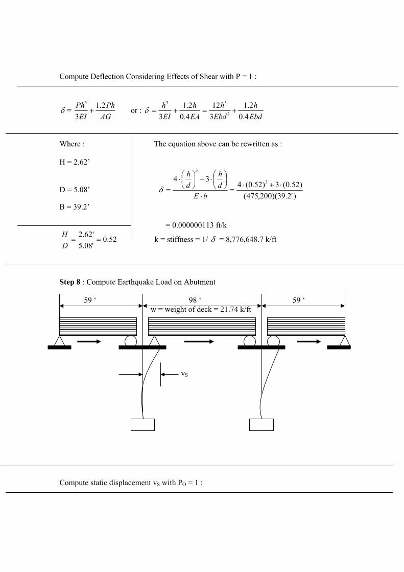
Compute Deflection Considering Effects of Shear with P = 1 :

=AG

Ph

EI

Ph 2.13

or : Ebd

hhh

EbdEAEI

h 2.1122.1 33

3 4.034.03 3

Where : The equation above can be rewritten as :

= 2.62’H

bEdd

34 hh3

D = 5.08’ )'2.39)(200,475(

)52.0(3)52.0(4 3

B = 39.2’

= 0.000000113 ft/k

52.0'08.5'62.2H k = stiffness = 1/

D = 8,776,648.7 k/ft

tep 8 : Compute Earthquake Load on Abutment

59 ‘ 98 ‘ 59 ‘

vS

ompute static displacement vS with PO = 1 :

S

w = weight of deck = 21.74 k/ft

C

VS = k

LPO = ftk

ft)0.98)(1( = 11.17 x 10 /7.8776648

Compute single-mode factors

-6

,, (AASHTO Division I-A 5.3) = vSL = (11.17 x 10 –6)(98) = 1.09 x 10 –3 ft2dxxvS

L )(0

= )(0

= 23.80 x 10 ft k vxw S wdxx)( = (1.09 x 10 ft )(21.74 k/ft)

–3

L –3 2

= = (23.80 x 10-3)(11.17 x 10-6)= 265.82 x 10 ft k

Co ation :

SSL vdxxvxw 20 )()(

-9 2

mpute period of oscill

)1009.1)(sec/2.32)(1(1080.262T = 2 5

62

29

xftk

kftx

gPO

3 sec

ompute Elastic Seismic Response Coefficient :

= Site coefficient = 1.2 (step 1)

= 0.017

C

A = Acceleration Coefficient = 0.15 (Given)

S

CS = 32

2.1

T

AS = 32

)2.1)(15.0(2.1 = 30173.0

.23

AASHTO Division I-A 5.2.1 states that CS need not exceed 2.5A :

CS = 2.5A = (2.5)(0.15) = 0.375 < 3.23 Use : CS = 0.375

Compute equivalent static earthquake loading :

Pe(x) = )()( xvxw SSC

= 9

3

1080.265)375.01080.23(

x

kxftx x (21.74 k /ft)(11.17 x 10-6)

= 8.160 k / ft

acting on abutment :

Y

Compute force

V = 0.2

)98)(/160.8()( ftftkLxpe

RSTEM

= 399.84 k

tep 9 : Compute Shears and Moments

VY 6’

PAE.6’

3.1’

Previously Determined Values

NOTE :

For all loads Wi and DL there is a

ding load kVWi and kVDL

rd

S

8”12 ”

DL

5

1.31’

correspon

acting upward (kV > 0) or downwa

(kV < 0).

KhW2

W2

A

0.225

W1 = 20.0 k ,kV = 0.09

Step 6

AE = 4.1189 PA = 4.1189(15.57 k /Pair) = 64.13 k/pair step 4

step 8

Y = (399.84 k) / 9 pairs of piles

kV) kV > 0

+ 20.0 k + 18.0 k )(1-0.09) -73.71 k

V < 0

= - (43.0 k + 20.0 k + 18.0 k)(1 + 0.09) -88.29 k

= (0.225)(43.0 k) + (0.225)(20.0 k) + (0.225)(18) + 44.43 + 64.13

F =

DL = 43.0 k , W2 = 18 k , kh =

Active pressure acting on stem :

PA = 15.57 k / pair

P

Superstructure loads acting on a pair of piles :

VY = 399.84 k

V

= 44.43 k

V= 0: -(DL + W1 + W2)(1-

= - (43.0 k

V= 0: -(DL + W1 + W2 )(1+kV) k

H = 0: khDL + khW1 + khW2 +VY + PAE

126.79 k

Axial Force:

ApilesBetDist. ween

V = MAX

ft

k

0.929.88 = FA = 9.81 k/ft

Force :

V =

Shear

pilesBetwDist. een

H = ft

k

0.979.126 = V = 14.10 k / ft

= 0: h

5.6VY+ 1.0DL (1+kV) + 3.1PAE + 6khW1 + 2W2kh – 0.67W1(1+ kV)

MA [k < 0][kV>0]

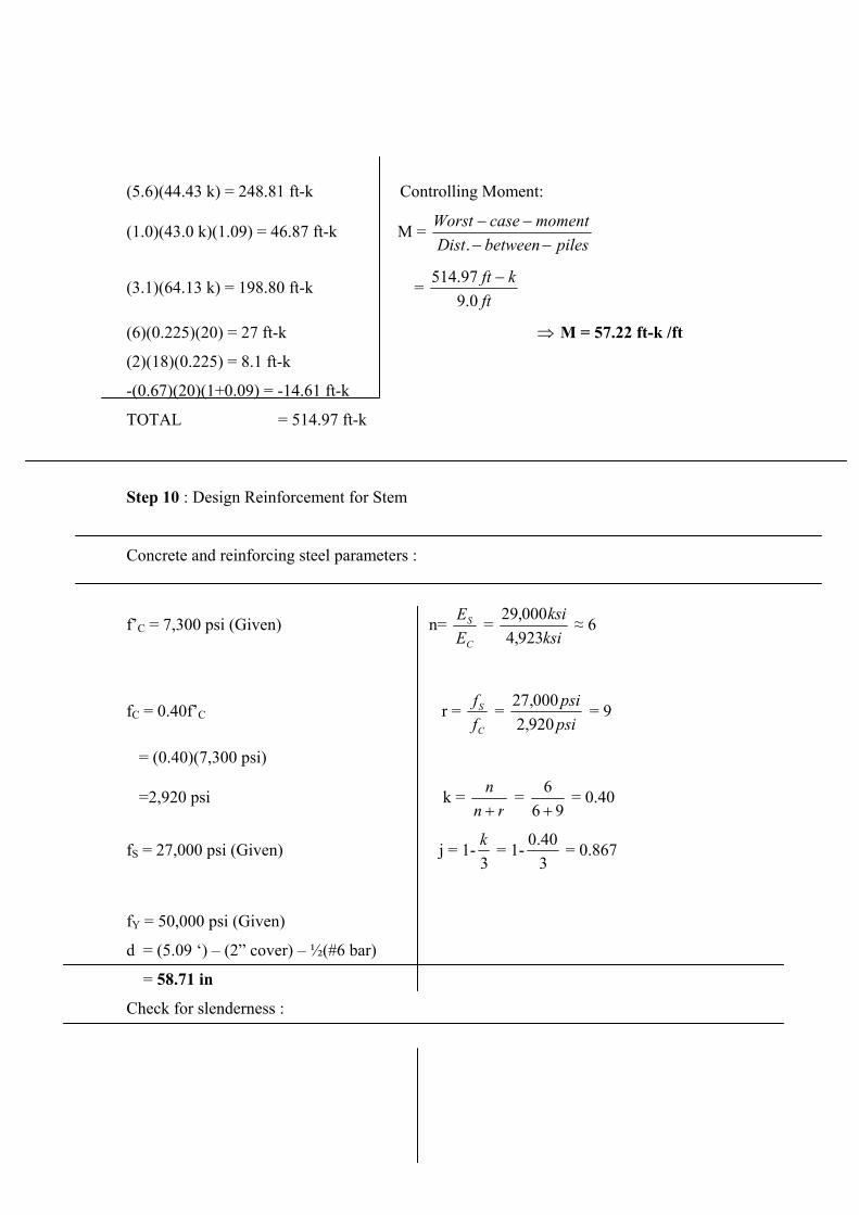
.0)(43.0 k)(1.09) = 46.87 ft-k M =

(5.6)(44.43 k) = 248.81 ft-k Controlling Moment:

(1piles

momentcaseWorst

betweenDist.

(3.1)(64.13 k) = 198.80 ft-k = ft

kft

0.997.514

(6)(0.225)(20) = 27 ft-k M = 57.22 ft-k /ft

(2)(18)(0.225) = 8.1 ft-k

.61 ft-k

14.97 ft-k

tep 10 : Design Reinforcement for Stem

n=

-(0.67)(20)(1+0.09) = -14

TOTAL = 5

S

Concrete and reinforcing steel parameters :

f’C = 7,300 psi (Given)C

S

E

E = ksi

ksi

923,4000,29 6

fC = 0.40f’C r = C

S

f

f = psi

psi

920,2000,27 = 9

=2,920 psi k =

= (0.40)(7,300 psi)

rn

n = 96

6 = 0.40

i (GfS = 27,000 ps iven) j = 1-3k

340.0= 1- = 0.867

= (5.09 ‘) – (2” cover) – ½(#6 bar)

fY = 50,000 psi (Given)

d

= 58.71 in

Check for slenderness :

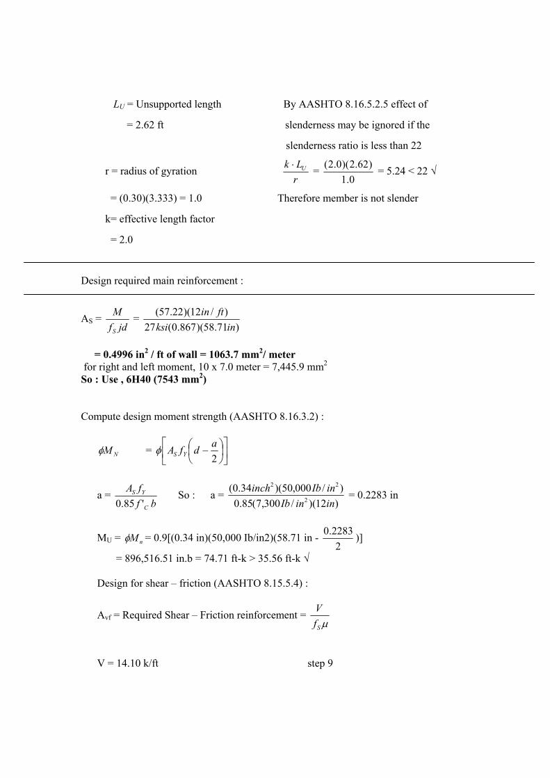
LU = Unsupported length By AASHTO 8.16.5.2.5 effect of

= 2.62 ft slenderness may be ignored if the

r = radius of gyration

slenderness ratio is less than 22

r

Lk U = 0.1

)62.2)(0.2( = 5.24 < 22

= (0.30)(3.333) = 1.0 Therefore member is not slender

k= effective length factor

Des n ed main reinforcement :

= 2.0

ig requir

AS = jdf

M = )71.58)(867.0(27

)/12)(22.57( ftin

S inksi

2 / ft of wall = 1063.7 mm2/ meterfor right and left moment, 10 x 7.0 meter = 7,445.9 mm2

o : Use , 6H40 (7543 mm2)

= 0.4996 in

S

Compute design moment strength (AASHTO 8.16.3.2) :

NM = 2

dfA YS

a

a = )12)(/300,7(85.0)/000,50)(34.

2

22

ininIb

inIbinch = 0.2283 in 0(bf

fA YS

C'85.0So : a =

nM = 0.9[(0.34 in)(50,000 Ib/in2)(58.71 in - 2

228MU = .0

= 896,516.51 in.b = 74.71 ft-k > 35.56 ft-k

3 )]

Design for shear – friction (AASHTO 8.15.5.4) :

Sf

VAvf = Required Shear – Friction reinforcement =

V = 14.10 k/ft step 9

fS = 27 ksi (Given)

= 0.60 (AASHTO 8.15.5.4.3(c)) = (0.60)(1.0)

Avf = )60(27

= 0.87 in / ft of wall = 1853.04 mm.0

/10.14 ftk 2 / meter

H20-150 (2095 mm2)

Temperature Steel: ch2)

2

# 5 bars @ 12 inch (0.31 in

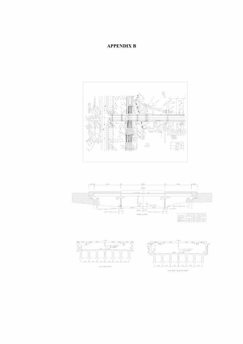
APPENDIX B

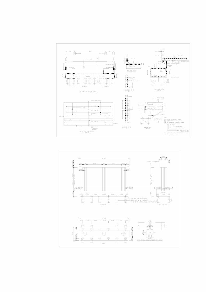
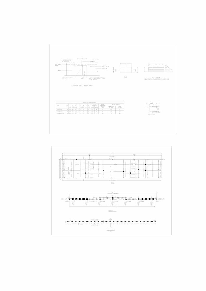
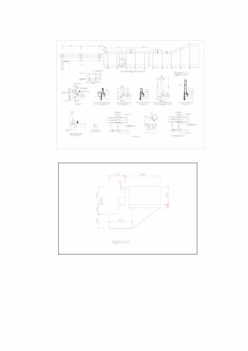
APPENDIX C

Data for El Centro 1940 North South Component (Peknold Version) 1559 points at equal spacing of 0.02 sec "Points are listed in the format of 8F10.5, i.e., 8 points across in" a row with 5 decimal places The units are (g) *** Begin data *** 0.00630 0.00364 0.00099 0.00428 0.00758 0.010870.00682 0.00277 -0.00128 0.00368 0.00864 0.01360 0.00727 0.000940.00420 0.00221 0.00021 0.00444 0.00867 0.01290 0.01713 -0.00343 -0.02400 -0.00992 0.00416 0.00528 0.01653 0.02779 0.03904 0.024490.00995 0.00961 0.00926 0.00892 -0.00486 -0.01864 -0.03242 -0.03365 -0.05723 -0.04534 -0.03346 -0.03201 -0.03056 -0.02911 -0.02766 -0.04116 -0.05466 -0.06816 -0.08166 -0.06846 -0.05527 -0.04208 -0.04259 -0.04311 -0.02428 -0.00545 0.01338 0.03221 0.05104 0.06987 0.08870 0.045240.00179 -0.04167 -0.08513 -0.12858 -0.17204 -0.12908 -0.08613 -0.08902 -0.09192 -0.09482 -0.09324 -0.09166 -0.09478 -0.09789 -0.12902 -0.07652 -0.02401 0.02849 0.08099 0.13350 0.18600 0.23850 0.21993 0.201350.18277 0.16420 0.14562 0.16143 0.17725 0.13215 0.08705 0.04196 -0.00314 -0.04824 -0.09334 -0.13843 -0.18353 -0.22863 -0.27372 -0.31882 -0.25024 -0.18166 -0.11309 -0.04451 0.02407 0.09265 0.16123 0.229810.29839 0.23197 0.16554 0.09912 0.03270 -0.03372 -0.10014 -0.16656 -0.23299 -0.29941 -0.00421 0.29099 0.22380 0.15662 0.08943 0.02224 -0.04495 0.01834 0.08163 0.14491 0.20820 0.18973 0.17125 0.137590.10393 0.07027 0.03661 0.00295 -0.03071 -0.00561 0.01948 0.044580.06468 0.08478 0.10487 0.05895 0.01303 -0.03289 -0.07882 -0.035560.00771 0.05097

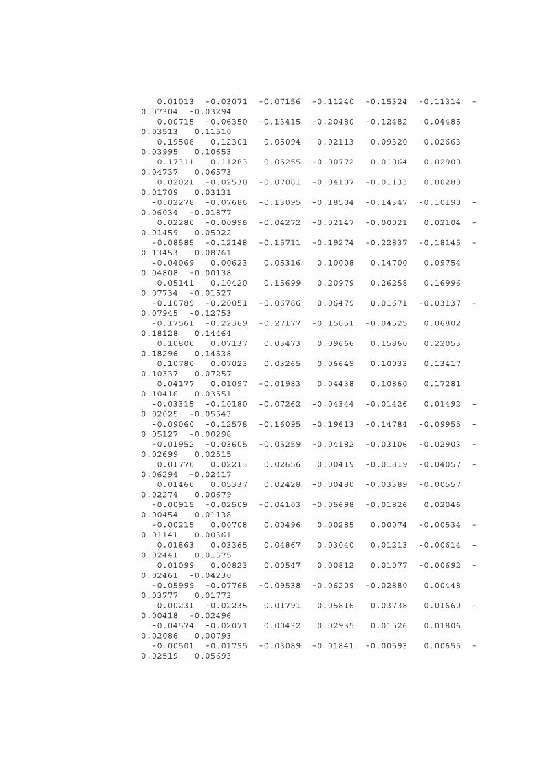
0.01013 -0.03071 -0.07156 -0.11240 -0.15324 -0.11314 -0.07304 -0.03294 0.00715 -0.06350 -0.13415 -0.20480 -0.12482 -0.044850.03513 0.11510 0.19508 0.12301 0.05094 -0.02113 -0.09320 -0.026630.03995 0.10653 0.17311 0.11283 0.05255 -0.00772 0.01064 0.029000.04737 0.06573 0.02021 -0.02530 -0.07081 -0.04107 -0.01133 0.002880.01709 0.03131 -0.02278 -0.07686 -0.13095 -0.18504 -0.14347 -0.10190 -0.06034 -0.01877 0.02280 -0.00996 -0.04272 -0.02147 -0.00021 0.02104 -0.01459 -0.05022 -0.08585 -0.12148 -0.15711 -0.19274 -0.22837 -0.18145 -0.13453 -0.08761 -0.04069 0.00623 0.05316 0.10008 0.14700 0.097540.04808 -0.00138 0.05141 0.10420 0.15699 0.20979 0.26258 0.169960.07734 -0.01527 -0.10789 -0.20051 -0.06786 0.06479 0.01671 -0.03137 -0.07945 -0.12753 -0.17561 -0.22369 -0.27177 -0.15851 -0.04525 0.068020.18128 0.14464 0.10800 0.07137 0.03473 0.09666 0.15860 0.220530.18296 0.14538 0.10780 0.07023 0.03265 0.06649 0.10033 0.134170.10337 0.07257 0.04177 0.01097 -0.01983 0.04438 0.10860 0.172810.10416 0.03551 -0.03315 -0.10180 -0.07262 -0.04344 -0.01426 0.01492 -0.02025 -0.05543 -0.09060 -0.12578 -0.16095 -0.19613 -0.14784 -0.09955 -0.05127 -0.00298 -0.01952 -0.03605 -0.05259 -0.04182 -0.03106 -0.02903 -0.02699 0.02515 0.01770 0.02213 0.02656 0.00419 -0.01819 -0.04057 -0.06294 -0.02417 0.01460 0.05337 0.02428 -0.00480 -0.03389 -0.005570.02274 0.00679 -0.00915 -0.02509 -0.04103 -0.05698 -0.01826 0.020460.00454 -0.01138 -0.00215 0.00708 0.00496 0.00285 0.00074 -0.00534 -0.01141 0.00361 0.01863 0.03365 0.04867 0.03040 0.01213 -0.00614 -0.02441 0.01375 0.01099 0.00823 0.00547 0.00812 0.01077 -0.00692 -0.02461 -0.04230 -0.05999 -0.07768 -0.09538 -0.06209 -0.02880 0.004480.03777 0.01773 -0.00231 -0.02235 0.01791 0.05816 0.03738 0.01660 -0.00418 -0.02496 -0.04574 -0.02071 0.00432 0.02935 0.01526 0.018060.02086 0.00793 -0.00501 -0.01795 -0.03089 -0.01841 -0.00593 0.00655 -0.02519 -0.05693

-0.04045 -0.02398 -0.00750 0.00897 0.00384 -0.00129 -0.00642 -0.01156 -0.02619 -0.04082 -0.05545 -0.04366 -0.03188 -0.06964 -0.05634 -0.04303 -0.02972 -0.01642 -0.00311 0.01020 0.02350 0.036810.05011 0.02436 -0.00139 -0.02714 -0.00309 0.02096 0.04501 0.069060.05773 0.04640 0.03507 0.03357 0.03207 0.03057 0.03250 0.034440.03637 0.01348 -0.00942 -0.03231 -0.02997 -0.03095 -0.03192 -0.02588 -0.01984 -0.01379 -0.00775 -0.01449 -0.02123 0.01523 0.05170 0.088160.12463 0.16109 0.12987 0.09864 0.06741 0.03618 0.00495 0.004200.00345 0.00269 -0.05922 -0.12112 -0.18303 -0.12043 -0.05782 0.004790.06740 0.13001 0.08373 0.03745 0.06979 0.10213 -0.03517 -0.17247 -0.13763 -0.10278 -0.06794 -0.03310 -0.03647 -0.03984 -0.00517 0.029500.06417 0.09883 0.13350 0.05924 -0.01503 -0.08929 -0.16355 -0.060960.04164 0.01551 -0.01061 -0.03674 -0.06287 -0.08899 -0.05430 -0.019610.01508 0.04977 0.08446 0.05023 0.01600 -0.01823 -0.05246 -0.08669 -0.06769 -0.04870 -0.02970 -0.01071 0.00829 -0.00314 0.02966 0.06246 -0.00234 -0.06714 -0.04051 -0.01388 0.01274 0.00805 0.03024 0.052430.02351 -0.00541 -0.03432 -0.06324 -0.09215 -0.12107 -0.08450 -0.04794 -0.01137 0.02520 0.06177 0.04028 0.01880 0.04456 0.07032 0.096080.12184 0.06350 0.00517 -0.05317 -0.03124 -0.00930 0.01263 0.034570.03283 0.03109 0.02935 0.04511 0.06087 0.07663 0.09239 0.057420.02245 -0.01252 0.00680 0.02611 0.04543 0.01571 -0.01402 -0.04374 -0.07347 -0.03990 -0.00633 0.02724 0.06080 0.03669 0.01258 -0.01153 -0.03564 -0.00677 0.02210 0.05098 0.07985 0.06915 0.05845 0.047750.03706 0.02636 0.05822 0.09009 0.12196 0.10069 0.07943 0.058160.03689 0.01563 -0.00564 -0.02690 -0.04817 -0.06944 -0.09070 -0.11197 -0.11521 -0.11846 -0.12170 -0.12494 -0.16500 -0.20505 -0.15713 -0.10921 -0.06129 -0.01337 0.03455 0.08247 0.07576 0.06906 0.06236 0.087350.11235 0.13734 0.12175 0.10616 0.09057 0.07498 0.08011 0.085240.09037 0.06208

0.03378 0.00549 -0.02281 -0.05444 -0.04030 -0.02615 -0.01201 -0.02028 -0.02855 -0.06243 -0.03524 -0.00805 -0.04948 -0.03643 -0.02337 -0.03368 -0.01879 -0.00389 0.01100 0.02589 0.01446 0.00303 -0.00840 0.00463 0.01766 0.03069 0.04372 0.02165 -0.00042 -0.02249 -0.04456 -0.03638 -0.02819 -0.02001 -0.01182 -0.02445 -0.03707 -0.04969 -0.05882 -0.06795 -0.07707 -0.08620 -0.09533 -0.06276 -0.03018 0.002390.03496 0.04399 0.05301 0.03176 0.01051 -0.01073 -0.03198 -0.053230.00186 0.05696 0.01985 -0.01726 -0.05438 -0.01204 0.03031 0.072650.11499 0.07237 0.02975 -0.01288 0.01212 0.03711 0.03517 0.033230.01853 0.00383 0.00342 -0.02181 -0.04704 -0.07227 -0.09750 -0.12273 -0.08317 -0.04362 -0.00407 0.03549 0.07504 0.11460 0.07769 0.040780.00387 0.00284 0.00182 -0.05513 0.04732 0.05223 0.05715 0.062060.06698 0.07189 0.02705 -0.01779 -0.06263 -0.10747 -0.15232 -0.12591 -0.09950 -0.07309 -0.04668 -0.02027 0.00614 0.03255 0.00859 -0.01537 -0.03932 -0.06328 -0.03322 -0.00315 0.02691 0.01196 -0.00300 0.003350.00970 0.01605 0.02239 0.04215 0.06191 0.08167 0.03477 -0.01212 -0.01309 -0.01407 -0.05274 -0.02544 0.00186 0.02916 0.05646 0.083760.01754 -0.04869 -0.02074 0.00722 0.03517 -0.00528 -0.04572 -0.08617 -0.06960 -0.05303 -0.03646 -0.01989 -0.00332 0.01325 0.02982 0.01101 -0.00781 -0.02662 -0.00563 0.01536 0.03635 0.05734 0.03159 0.00584 -0.01992 -0.00201 0.01589 -0.01024 -0.03636 -0.06249 -0.04780 -0.03311 -0.04941 -0.06570 -0.08200 -0.04980 -0.01760 0.01460 0.04680 0.079000.04750 0.01600 -0.01550 -0.00102 0.01347 0.02795 0.04244 0.056920.03781 0.01870 -0.00041 -0.01952 -0.00427 0.01098 0.02623 0.041480.01821 -0.00506 -0.00874 -0.03726 -0.06579 -0.02600 0.01380 0.053590.09338 0.05883 0.02429 -0.01026 -0.04480 -0.01083 -0.01869 -0.02655 -0.03441 -0.02503 -0.01564 -0.00626 -0.01009 -0.01392 0.01490 0.043720.03463 0.02098 0.00733 -0.00632 -0.01997 0.00767 0.03532 0.034090.03287 0.03164

0.02403 0.01642 0.00982 0.00322 -0.00339 0.02202 -0.01941 -0.06085 -0.10228 -0.07847 -0.05466 -0.03084 -0.00703 0.016780.01946 0.02214 0.02483 0.01809 -0.00202 -0.02213 -0.00278 0.016560.03590 0.05525 0.07459 0.06203 0.04948 0.03692 -0.00145 0.045990.04079 0.03558 0.03037 0.03626 0.04215 0.04803 0.05392 0.049470.04502 0.04056 0.03611 0.03166 0.00614 -0.01937 -0.04489 -0.07040 -0.09592 -0.07745 -0.05899 -0.04052 -0.02206 -0.00359 0.01487 0.010050.00523 0.00041 -0.00441 -0.00923 -0.01189 -0.01523 -0.01856 -0.02190 -0.00983 0.00224 0.01431 0.00335 -0.00760 -0.01856 -0.00737 0.003830.01502 0.02622 0.01016 -0.00590 -0.02196 -0.00121 0.01953 0.040270.02826 0.01625 0.00424 0.00196 -0.00031 -0.00258 -0.00486 -0.00713 -0.00941 -0.01168 -0.01396 -0.01750 -0.02104 -0.02458 -0.02813 -0.03167 -0.03521 -0.04205 -0.04889 -0.03559 -0.02229 -0.00899 0.00431 0.017620.00714 -0.00334 -0.01383 0.01314 0.04011 0.06708 0.04820 0.029320.01043 -0.00845 -0.02733 -0.04621 -0.03155 -0.01688 -0.00222 0.012440.02683 0.04121 0.05559 0.03253 0.00946 -0.01360 -0.01432 -0.01504 -0.01576 -0.04209 -0.02685 -0.01161 0.00363 0.01887 0.03411 0.031150.02819 0.02917 0.03015 0.03113 0.00388 -0.02337 -0.05062 -0.03820 -0.02579 -0.01337 -0.00095 0.01146 0.02388 0.03629 0.01047 -0.01535 -0.04117 -0.06699 -0.05207 -0.03715 -0.02222 -0.00730 0.00762 0.022540.03747 0.04001 0.04256 0.04507 0.04759 0.05010 0.04545 0.040800.02876 0.01671 0.00467 -0.00738 -0.00116 0.00506 0.01128 0.01750 -0.00211 -0.02173 -0.04135 -0.06096 -0.08058 -0.06995 -0.05931 -0.04868 -0.03805 -0.02557 -0.01310 -0.00063 0.01185 0.02432 0.03680 0.049270.02974 0.01021 -0.00932 -0.02884 -0.04837 -0.06790 -0.04862 -0.02934 -0.01006 0.00922 0.02851 0.04779 0.02456 0.00133 -0.02190 -0.04513 -0.06836 -0.04978 -0.03120 -0.01262 0.00596 0.02453 0.04311 0.061690.08027 0.09885 0.06452 0.03019 -0.00414 -0.03848 -0.07281 -0.05999 -0.04717 -0.03435

-0.03231 -0.03028 -0.02824 -0.00396 0.02032 0.00313 -0.01406 -0.03124 -0.04843 -0.06562 -0.05132 -0.03702 -0.02272 -0.008430.00587 0.02017 0.02698 0.03379 0.04061 0.04742 0.05423 0.035350.01647 0.01622 0.01598 0.01574 0.00747 -0.00080 -0.00907 0.000720.01051 0.02030 0.03009 0.03989 0.03478 0.02967 0.02457 0.030750.03694 0.04313 0.04931 0.05550 0.06168 -0.00526 -0.07220 -0.06336 -0.05451 -0.04566 -0.03681 -0.03678 -0.03675 -0.03672 -0.01765 0.001430.02051 0.03958 0.05866 0.03556 0.01245 -0.01066 -0.03376 -0.05687 -0.04502 -0.03317 -0.02131 -0.00946 0.00239 -0.00208 -0.00654 -0.01101 -0.01548 -0.01200 -0.00851 -0.00503 -0.00154 0.00195 0.00051 -0.000920.01135 0.02363 0.03590 0.04818 0.06045 0.07273 0.02847 -0.01579 -0.06004 -0.05069 -0.04134 -0.03199 -0.03135 -0.03071 -0.03007 -0.01863 -0.00719 0.00425 0.01570 0.02714 0.03858 0.02975 0.02092 0.023340.02576 0.02819 0.03061 0.03304 0.01371 -0.00561 -0.02494 -0.02208 -0.01923 -0.01638 -0.01353 -0.01261 -0.01170 -0.00169 0.00833 0.018340.02835 0.03836 0.04838 0.03749 0.02660 0.01571 0.00482 -0.00607 -0.01696 -0.00780 0.00136 0.01052 0.01968 0.02884 -0.00504 -0.03893 -0.02342 -0.00791 0.00759 0.02310 0.00707 -0.00895 -0.02498 -0.04100 -0.05703 -0.02920 -0.00137 0.02645 0.05428 0.03587 0.01746 -0.00096 -0.01937 -0.03778 -0.02281 -0.00784 0.00713 0.02210 0.03707 0.052040.06701 0.08198 0.03085 -0.02027 -0.07140 -0.12253 -0.08644 -0.05035 -0.01426 0.02183 0.05792 0.09400 0.13009 0.03611 -0.05787 -0.04802 -0.03817 -0.02832 -0.01846 -0.00861 -0.03652 -0.06444 -0.06169 -0.05894 -0.05618 -0.06073 -0.06528 -0.04628 -0.02728 -0.00829 0.01071 0.029700.03138 0.03306 0.03474 0.03642 0.04574 0.05506 0.06439 0.073710.08303 0.03605 -0.01092 -0.05790 -0.04696 -0.03602 -0.02508 -0.01414 -0.03561 -0.05708 -0.07855 -0.06304 -0.04753 -0.03203 -0.01652 -0.001020.00922 0.01946 0.02970 0.03993 0.05017 0.06041 0.07065 0.08089 -0.00192 -0.08473

-0.07032 -0.05590 -0.04148 -0.05296 -0.06443 -0.07590 -0.08738 -0.09885 -0.06798 -0.03710 -0.00623 0.02465 0.05553 0.086400.11728 0.14815 0.08715 0.02615 -0.03485 -0.09584 -0.07100 -0.04616 -0.02132 0.00353 0.02837 0.05321 -0.00469 -0.06258 -0.12048 -0.09960 -0.07872 -0.05784 -0.03696 -0.01608 0.00480 0.02568 0.04656 0.067440.08832 0.10920 0.13008 0.10995 0.08982 0.06969 0.04955 0.040060.03056 0.02107 0.01158 0.00780 0.00402 0.00024 -0.00354 -0.00732 -0.01110 -0.00780 -0.00450 -0.00120 0.00210 0.00540 -0.00831 -0.02203 -0.03575 -0.04947 -0.06319 -0.05046 -0.03773 -0.02500 -0.01227 0.000460.00482 0.00919 0.01355 0.01791 0.02228 0.00883 -0.00462 -0.01807 -0.03152 -0.02276 -0.01401 -0.00526 0.00350 0.01225 0.02101 0.014370.00773 0.00110 0.00823 0.01537 0.02251 0.01713 0.01175 0.006370.01376 0.02114 0.02852 0.03591 0.04329 0.03458 0.02587 0.017150.00844 -0.00027 -0.00898 -0.00126 0.00645 0.01417 0.02039 0.026610.03283 0.03905 0.04527 0.03639 0.02750 0.01862 0.00974 0.00086 -0.01333 -0.02752 -0.04171 -0.02812 -0.01453 -0.00094 0.01264 0.026230.01690 0.00756 -0.00177 -0.01111 -0.02044 -0.02977 -0.03911 -0.02442 -0.00973 0.00496 0.01965 0.03434 0.02054 0.00674 -0.00706 -0.02086 -0.03466 -0.02663 -0.01860 -0.01057 -0.00254 -0.00063 0.00128 0.003190.00510 0.00999 0.01488 0.00791 0.00093 -0.00605 0.00342 0.012880.02235 0.03181 0.04128 0.02707 0.01287 -0.00134 -0.01554 -0.02975 -0.04395 -0.03612 -0.02828 -0.02044 -0.01260 -0.00476 0.00307 0.010910.00984 0.00876 0.00768 0.00661 0.01234 0.01807 0.02380 0.029530.03526 0.02784 0.02042 0.01300 -0.03415 -0.00628 -0.00621 -0.00615 -0.00609 -0.00602 -0.00596 -0.00590 -0.00583 -0.00577 -0.00571 -0.00564 -0.00558 -0.00552 -0.00545 -0.00539 -0.00532 -0.00526 -0.00520 -0.00513 -0.00507 -0.00501 -0.00494 -0.00488 -0.00482 -0.00475 -0.00469 -0.00463 -0.00456 -0.00450 -0.00444 -0.00437 -0.00431 -0.00425 -0.00418 -0.00412 -0.00406 -0.00399

-0.00393 -0.00387 -0.00380 -0.00374 -0.00368 -0.00361 -0.00355 -0.00349 -0.00342 -0.00336 -0.00330 -0.00323 -0.00317 -0.00311 -0.00304 -0.00298 -0.00292 -0.00285 -0.00279 -0.00273 -0.00266 -0.00260 -0.00254 -0.00247 -0.00241 -0.00235 -0.00228 -0.00222 -0.00216 -0.00209 -0.00203 -0.00197 -0.00190 -0.00184 -0.00178 -0.00171 -0.00165 -0.00158 -0.00152 -0.00146 -0.00139 -0.00133 -0.00127 -0.00120 -0.00114 -0.00108 -0.00101 -0.00095 -0.00089 -0.00082 -0.00076 -0.00070 -0.00063 -0.00057 -0.00051 -0.00044 -0.00038 -0.00032 -0.00025 -0.00019 -0.00013 -0.000060.00000*** End Data ***