Comparison Geometry - MSRIlibrary.msri.org/books/Book30/files/petersen.pdf · Comparison Geometry...
36
Transcript of Comparison Geometry - MSRIlibrary.msri.org/books/Book30/files/petersen.pdf · Comparison Geometry...
Comparison GeometryMSRI PublicationsVolume 30, 1997
Convergence Theorems in Riemannian Geometry
PETER PETERSEN
Abstract. This is a survey on the convergence theory developed �rst by
Cheeger and Gromov. In their theory one is concerned with the compact-
ness of the class of riemannian manifolds with bounded curvature and lower
bound on the injectivity radius. We explain and give proofs of almost all
the major results, including Anderson's generalizations to the case where
all one has is bounded Ricci curvature. The exposition is streamlined by the
introduction of a norm for riemannian manifolds, which makes the theory
more like that of H�older and Sobolev spaces.
1. Introduction
This paper is an outgrowth of a talk given in October 1993 at MSRI and
a graduate course o�ered in the Spring of 1994 at UCLA. The purpose is to
introduce readers to the convergence theory of riemannian manifolds not so much
through a traditional survey article, but by rigorously proving most of the key
theorems in the subject. For a broader survey of this subject, and how it can be
applied to various problems, we refer the reader to [Anderson 1993].
The prerequisites for this paper are some basic knowledge of riemannian geom-
etry, Gromov{Hausdor� convergence and elliptic regularity theory. In particular,
the reader should be familiar with the comparison geometry found in [Karcher
1989], for example. For Gromov{Hausdor� convergence, it su�ces to read Sec-
tion 6 in [Gromov 1981a] or Section 1 in [Petersen 1993]. In regard to elliptic
theory, we have an appendix that contains all the results we need, together with
proofs of those theorems that are not explicitly stated in [Gilbarg and Trudinger
1983].
In Section 2 we introduce the concept of (pointed) Ck+� convergence of rie-
mannian manifolds. This introduces a natural topology on (pointed) riemannian
manifolds and immediately raises the question of which \subsets" are precom-
pact. To answer this, we use, for the �rst time in the literature, the idea that
a riemannian manifold in a natural way has a Ck+� norm for each �xed scale
Partially supported by NSF and NYI grants.
167

168 PETER PETERSEN
r > 0. This norm is a quantitative version of the de�nition of a manifold. It is
basically computed by �nding atlases of charts from r-balls in Rn into the man-
ifold and then, for each of these atlases, by computing the largest Ck+� norm
of the metric coe�cients in these charts, and for compatibility reasons, also the
largest Ck+1+� norm of the transition functions. The scale r is an integral part
of the de�nition, so that Rn becomes the only space that has zero norm on all
scales, while at manifolds have zero norm on small scales, and non at manifolds
have the property that the norm goes to zero as the scale goes to zero. The norm
concept is dual to the usual radii concepts in geometry, but has nicer properties.
We have found this norm concept quite natural to work with: It gives, for
instance, a very elegant formulation of what we call The Fundamental Theorem
of Convergence Theory. This theorem is completely analogous to the classical
Arzela{Ascoli theorem, and says that, for each �xed scale r, the class of rie-
mannian n-manifolds of Ck+� norm � Q is compact in the Ck+� topology for
� < �. The only place where we use Gromov{Hausdor� convergence is in the
proof of this theorem. Aside from the new concept of norm and the use of
Gromov{Hausdor� convergence, the proof of this fundamental theorem is essen-
tially contained in [Cheeger 1970].
In Section 3 we use the Fundamental Theorem to prove the Compactness
Theorem of Cheeger and Gromov for manifolds of bounded curvature, as it is
stated in [Gromov 1981b]. In addition we give a new proof by contradiction of
Cheeger's lemma on the injectivity radius, using convergence techniques. Finally,
we give S.-H. Zhu's proof of the compactness of the class of n-manifolds with
lower sectional curvature bounds and lower injectivity radius bounds.
The theory really picks up speed in Section 4, where we introduce Lp;k norms
on the scale of r, using harmonic coordinates. It is at this point that we need to
use elliptic regularity theory. The idea of using harmonic coordinates, rather than
just general coordinates, makes a big di�erence in the theory, since it makes the
norm a locally realizable number. This is basically a consequence of the fact that
we don't have to worry about the norms of transition functions. Our \harmonic"
norm is, of course, dual to Anderson's harmonic radius, but we again �nd that
the norm idea has some important technical advantages over the use of harmonic
radius.
Most of Anderson's convergence results are proved in Section 5. They are all
generalizations of the Cheeger{Gromov Compactness Theorem, but the proofs
are, in contrast, all by contradiction.
The �nal Section 6 has some applications of convergence theory to pinch-
ing problems in riemannian geometry. Some of the results in this section are
extensions of work in [Gao 1990].
CONVERGENCE THEOREMS IN RIEMANNIAN GEOMETRY 169
2. The Fundamentals
For a function f : ! Rh , where � Rn the H�older C�-constant 0 < � � 1
is de�ned as:
kfk� = supx;y2
jf(x)� f(y)jjx� yj� :
In other words, kfk� is the smallest constant C such that jf(x) � f(y)j �C jx � yj�. Notice that kfk1 is the best Lipschitz constant for f . If � Rn is
open, k � 0 is an integer, and 0 < � � 1, we de�ne the Ck+� norm of f as
kfkk+� = kfkCk +maxjjj=k
k@jfk�:
Here kfkCk is the usual Ck-norm and @j = @j11 � � � @jnn , where @i = @=@xi and
j = (j1; : : : ; jn) is a multi-index. Note that the norm kfkk+1 is not the same as
kfkCk+1 .
We denote by Ck+�() the space of functions with �nite (k + �)-norm. This
norm makes Ck+�() into a Banach space. The classical Arzela{Ascoli Theorem
says that for k + � > 0, 0 < � � 1, and l + � < k + �, any sequence satisfying
kfikk+� � � has a subsequence that converges in the l+�-topology to a function
f , with kfkk+� � �. Note that if � = 0 it is not necessarily true that f is Ck ,
but it will be Ck�1+1. We shall therefore always look at (k+�)-topologies with
0 < � � 1.
We can now de�ne Ck+� convergence of tensors on a given manifold M .
Namely, a sequence Ti of tensors on M is said to converge to T in the Ck+�-
topology if we can �nd a covering 's : Us ! Rn of coordinate charts so that
the overlap maps are at least Ck+1+� and all the components of the tensors
Ti converge in the Ck+� topology to the components of T in these coordinate
charts, considered as functions on '�(U�) � Rn . This convergence concept is
clearly independent of our choice of coordinates. Note that it is necessary for
the overlaps to be Ck+1+�, since the components of tensors are computed by
evaluating these tensors on the Ck+� �elds @=@xi and dxi.
In the sequel we shall restrict our attention to complete or closed riemannian
manifolds. Some of the theory can, with modi�cations, be generalized to in-
complete manifolds and manifolds with boundary. These generalizations, while
useful, are not very deep and can be found in the literature.
A pointed sequence (Mi; gi; pi) of riemannian n-manifolds with metrics gi,
and pi 2 Mi, is said to converge to a riemannian manifold (M; g; p) in the
pointed Ck+� topology if, for each R > 0, there is a domain in M containing
the open ball B(p;R) and embeddings fi : ! Mi, for large i, such that
fi() � B(pi; R) and the f�i gi converge to g in the Ck+� topology on . If we
can choose =M and fi() =Mi, we say that (Mi; gi) converges to (M; g) in
the Ck+�-topology. There is obviously no signi�cant di�erence between pointed
and unpointed topologies when all manifolds in use are closed.

170 PETER PETERSEN
It is very important to realize that this concept of Ck+� convergence is not
the same as the one we just de�ned for tensors on a given manifold M , even
when we are considering a sequence of riemannian metrics gi on the same space
M . This is because one can have a sequence of metrics gi and di�eomorphisms
fi :M !M such that ff�i gig converges while fgig does not converge.We say that a collection of riemannian n-manifolds is precompact in the
(pointed) Ck+� topology if any sequence in this collection has a subsequence that
is convergent in the (pointed) Ck+�-topology|in other words, if the (pointed)
Ck+�-closure is compact.
The rest of the paper is basically concerned with �nding reasonable (geomet-
ric) conditions that imply precompactness in some of these topologies. In order
to facilitate this task and ease the exposition a little, we need to introduce some
auxiliary concepts.
For a riemannian n-manifold we de�ne the Ck+�-norm on the scale of r > 0,
denoted k(M; g)kk+�;r, as the in�mum over all numbers Q � 0 such that we can
�nd coordinates charts 's : B(0; r) � Rn ! Us �M with these properties:
(n1) Every ball of radius � = 110e
�Qr is contained in some Us.
(n2) jd'�1s j � eQ and jd'sj � eQ on B(0; r).
(n3) rjjj+�k@jgs��k� � Q for all multi-indices j with 0 � jjj � k.
(n4) k'�1s � 'tkk+1+� � (10 + r) eQ on the domain of de�nition.
Here gs�� represents the metric components in the coordinates 's, considered
as functions on B(0; r) � Rn . The �rst condition is equivalent to saying that
� is a Lebesgue number for the covering fUsg. The second condition can be
rephrased as saying that the eigenvalues of gs�� with respect to the standard
euclidean metric lie between e�Q and eQ. This gives both a C0 bound for gs��and a uniform positive de�niteness for gs��.
If A is a subset of M , we can de�ne k(A; g)kk+�;r in a similar way, only
changing (n1) to say that all �-balls centered on A are contained in some Us. In
(n1) it would perhaps have been more natural to merely assume that the sets
Us cover M (or A). That, however, is not a desirable state of a�airs, because
this would put us in a situation where the norm k kk+�;r wouldn't necessarilybe realized by some Q. A fake but illustrative example is the sphere, covered by
two balls of radius r > �=2 centered at antipodal points. As r ! �=2 the sets
will approach a situation where they no longer cover the space.
From the de�nition it is clear that k(M; g)kk+�;r must be �nite for all r, whenM is closed. For open manifolds it would be more natural to have some weight
function f : M ! R, which allows for Q to get bigger as we go farther and
farther out on the manifold. We'll say a few more words about this later in this
section.
Example. If M = Rn with the canonical euclidean metric, then kMkk+�;r = 0
for all r. More generally, we can easily prove that k(M; g)kk+�;r = 0 for r �

CONVERGENCE THEOREMS IN RIEMANNIAN GEOMETRY 171
inj rad(M; g) if (M; g) is a at manifold. We shall see later in this section that
these properties characterize Rn and at manifolds in general.
With this example in mind, it is pretty clear that conditions (n1){(n3) say that
on a scale of r the metric on (M; g) is Q-close to the euclidean metric in the
Ck+� topology. Condition (n4) is a compatibility condition that ensures that
Ck+�-closeness to euclidean space means the same in all coordinates.
For a given Q and r we can in the usual fashion consider maximal atlases of
all charts satisfying (n1){(n4), but we won't use this much. Let us now turn to
some of the properties of this norm.
Proposition 2.1. Let (M; g) be a C1 riemannian n-manifold .
(i) k(A; �2g)kk+�;�r = k(A; g)kk+�;r; in other words the norm is scale invariant ,
for all A �M .
(ii) IfM is compact , then k(M; g)kk+�;r is �nite for all r; moreover , this number
depends continuously on r, and it tends to 0 as r ! 0.
(iii) If (Mi; gi; pi)! (M; g; p) in the pointed Ck+�-topology , then for any bounded
domain B �M we can �nd domains Bi �Mi such that
k(Bi; gi)kk+�;r ! k(B; g)kk+�;r for every r > 0:
When all spaces involved are closed manifolds we can set Bi =Mi and B =M .
Proof. (i) If we change g to �2g we can change charts 's : B(0; r) ! M to
's��1 (x) = '(��1x) : B(0; �r) ! M . Since we are also scaling the metric, this
means that conditions (n1){(n4) still hold with the same Q.
(ii) If, as in (i), we only change g to �2g, but do not scale in euclidean space,
we get
for � < 1; k(M;�2g)kk+�;r � Q� log�
for � > 1; k(M;�2g)kk+�;r � maxf�Q; Q+ log�g;where k(M; g)kk+�;r < Q. Thus
k(M; g)kk+�;��1r � maxf�Q; Q� log�; Q+ log�g:If, therefore, the norm is �nite for some r, it will be �nite for all r. Furthermore,
f(r) = k(M; g)kk+�;r is a function with the property that, for each r,
f(��1r) � h(�; f(r)) = maxf�f(r); f(r) � log�; f(r) + log �g;and f(r) = h(1; f(r)). If, therefore, ri ! r, we clearly have lim sup f(ri) � f(r),
since f(ri) = f (r (ri=r)) � g (r=ri; f(r)). Conversely, f(r) = f (ri r=ri) �h (ri=r; f(ri)) = max ff(ri) ri=r; f(ri)� log(ri=r); f(ri) + log(ri=r)g � f(ri) +
", for any " > 0 as ri ! r. Thus f(r) � lim inf f(ri), and we have established
continuity of f(r).
To see that k(M; g)kk+�;r ! 0 as r ! 0 just use exponential coordinates
exppi : B(0; r)! B(pi; r).
172 PETER PETERSEN
(iii) Fix r > 0 and B � M . Then choose embeddings fi : ! Mi such that
f�i gi converge to g and B � . De�ne Bi = fi(B).
For Q > k(B; g)kk+�;r, choose appropriate charts 's : B(0; r)!M satisfying
(n1){(n4), with B = A. Then 'si = fi � 's : B(0; r) ! Mi will satisfy (n1) and
(n4). Now, since f�i gi ! g in the Ck+�-topology, (n2) and (n3) will hold with a
Qi satisfying Qi ! Q as i!1. Thus lim sup k(Bi; g)kk+�;r � k(B; g)kk+�;r.Conversely, for large i and Q > lim inf k(Bi; gi)kk+�;r . We can choose charts
'si : B(0; r) ! Mi satisfying (n1){(n4) with Bi = A. Now consider 's =
f�1i � 'si : B(0; r) ! M . These charts will satisfy n1 and n4, and again n2 and
n3 for some Qi � Q, which can be chosen to converge to Q as i ! 1. Thus
lim inf k(Bi; gi)kk+�;r � k(B; g)kk+�;r. �
A few comments about our de�nition of k(M; g)kk+�;r are in order at this point.From a geometric point of view, it would probably have been nicer to assume
that our charts 's : B(p; r) � M ! � Rn , were de�ned on metric balls in
M rather than on Rn . The reason for not doing so is technical, but still worth
pondering. With revised charts, k(M; g)kk+�;r would de�nitely be 1 for large
r, unless (M; g) were euclidean space; even worse, our proof of (iii) would break
down, as the charts 'i � fi and ' � f�1i would not be de�ned on metric r-balls
but only on slightly smaller balls. We could partially avert these problems by
maximizing r for �xedQ, rather than minimizingQ for �xed r, and thereby de�ne
a (Q; k + �) radius rk+�;Q(M). This is exactly what was done in Anderson's
work on convergence, and it follows more closely the standard terminology in
riemannian geometry. But even with this de�nition, we still cannot conclude
that this radius concept varies continuously in the Ck+� topology for �xed Q.
All we get is that rk+�;Qi(Mi; gi) ! rk+�;Q(M; g) for some sequence Qi # Q,
where Q is chosen in advance. Our concept of norm, therefore, seems to behave
in a nicer manner from an analytic point of view. However, when it really
matters, the two viewpoints are more or less equivalent. We also think that the
norm concept is more natural, since it is a quantitative version of the qualitative
coordinate de�nition of a manifold with a riemannian structure.
Another issue is exactly how to de�ne the norm for noncompact manifolds.
The most natural thing to do would be to consider pointed spaces (M; g; p),
choose a nondecreasing weight function f(R), and assume kB(p;R))kk+�;r �f(R). Our whole theory can easily be worked out in this context, but for the
sake of brevity, we won't do this.
For noncompact spaces one can also use the norm concept to de�ne what it
should mean for a space to be asymptotically locally euclidean of order k + �|
namely, that it should satisfy k(M � B(p;R); g)kk+�;r ! 0 as R ! 1. Here
one can also re�ne this and assume that r should, in some way, depend on R.
Our next theorem is, in a way, as basic as our proposition, and in fact it
uses none of our basic properties. The proof, however, is a bit of a mouthful.
Nevertheless, the reader is urged to go through it carefully, because many of
CONVERGENCE THEOREMS IN RIEMANNIAN GEOMETRY 173
the subsequent corollaries are only true corollaries in the context of some of the
constructions in the proof.
Theorem 2.2 (Fundamental Theorem of Convergence Theory). For
given Q > 0, n � 2 integer , k+� > 0, and r > 0, consider the class Hk+�(n;Q; r)
of complete, pointed riemannian n-manifolds (M; g; p) with k(M; g)kk+�;r � Q.
Then Hk+�(n;Q; r) is compact in the pointed Ck+�-topology for all k+� < k+�.
Proof. We proceed in stages. First we make some general comments about
the charts we use. We then show that H = Hk+�(n;Q; r) is precompact in the
pointed Gromov{Hausdor� topology. Next we prove that H is compact in the
Gromov{Hausdor� topology. Finally we consider the statement of the theorem.
Setup: First �x K > Q. Whenever we select an M 2 H we shall assume that
it comes equipped with an atlas of charts satisfying (n1){(n4) with K in place
of Q. Thus we implicitly assume that all charts under consideration belong to
these atlases. We will, in consequence, only prove that limit spaces (M; g; p)
satisfy k(M; g)kk+�;r � K, but since K was arbitrary we still get (M; g; p) 2 H.We proceed by establishing several simple facts.
Fact 1. Every chart ' : B(0; r)! U �M 2 H satis�es
(a) d('(x1); '(x2)) � eK jx1 � x2j and(b) d('(x1); '(x2)) � minfe�K jx1 � x2j; e�K(2r � jx1j � jx2j)g,where d is distance measured in M , and j � j is the usual euclidean norm. The
condition jd'j � eK together with convexity of B(0; r) immediately implies (a).
For (b), �rst observe that if any segment from x1 to x2 lies in U , then jd'j � e�K
implies that d('(x1); '(x2)) � e�K jx1 � x2j. So we may assume that '(x1) and'(x2) are joined by a segment � : [0; 1] ! M that leaves U . Split � into
� : [0; t1)! U , and � : (t2; 1)! U such that �(ti) =2 U . Then we clearly have
d('(x1); '(x2)) = L(�) � L(�j[0;t1)) + L(�j(t2;1])� e�K
�L('�1 � �j[0;t1)) + L('�1 � �j(t2;1])
�� e�K(2r � jx1j � jx2j):
The last inequality follows from the fact that '�1�(0) = x1; '�1 ��(1) = x2 and
that '�1 � �(t) approaches the boundary of B(0; r) as t% t1, or t& t2.
Fact 2. Every chart ' : B(0; r) ! U � M 2 H, and hence any �-ball in M ,
where � = 110e
�Kr, can be covered by at most N(�=4)-balls, where N depends
only on n;K; r. Clearly there exists an N(n;K; r) such that B(0; r) can be
covered by at most Ne�K (�=4)-balls. Since ' : B(0; r)! U is a Lipschitz map
with Lipschitz constant � eK , we get the desired covering property.
Fact 3. Every ball B(x; l�=2) �M can be covered by � N l �=4-balls. For l = 1
we just proved this. Suppose we know that B(x; l�=2) is covered by B(x1; �=4),
. . . , B(xNl ; �=4). Then B(x; l�=2 + �=2) � SNi=1 B(xi; �). Now each B(xi; �)
174 PETER PETERSEN
can be covered by at most N�=4-balls; hence B(x; (l +1)�=2) can be covered by
� N N l = N l+1 �=4-balls.
Fact 4. H is precompact in the pointed Gromov{Hausdor� topology. This
is equivalent to asserting that, for each R > 0, the family of metric balls
B(p;R) � (M; g; p) 2 H is precompact in the Gromov{Hausdor� topology. This
claim is equivalent to showing that we can �nd a function N(") = N(";R;K; r; n)
such that each B(p;R) can contain at most N(") disjoint "-balls. To check this,
let B(x1; "); : : : ; B(xs; ") be a collection of disjoint balls in B(p;R). Suppose that
l�=2 < R � (l + 1)�=2; then the volume of B(p;R) is at most N (l+1) times the
maximal volume of (�=4)-ball, therefore at most N (l+1) times the maximal vol-
ume of a chart, therefore at most N (l+1)enK volB(0; r) � F (R) = F (R; n;K; r).
Conversely, each B(xi; ") lies in some chart ' : B(0; r) ! U �M whose preim-
age in B(0; r) contains an (e�K")-ball. Thus volB(pi; ") � e�2nK volB(0; "). All
in all we get F (R) � volB(p;R) � PvolB(pi; ") � s e�2nK volB(0; "). Thus
s � N(") = F (R)e2nK(volB(0; "))�1.
Now select a sequence (Mi; gi; pi) in H. From the previous considerations
we can assume that (Mi; gi; pi) ! (X; d; p) converge to some metric space in
the Gromov{Hausdor� topology. It will be necessary in many places to pass to
subsequences of (Mi; gi; pi) using various diagonal processes. Whenever this hap-
pens, we shall not reindex the family, but merely assume that the sequence was
chosen to have the desired properties from the beginning. For each (Mi; gi; pi)
choose charts 'is : B(0; r) ! Uis � Mi satisfying (n1){(n4). We can further-
more assume that the index set fsg = f1; 2; 3; 4; � � �g is the same for all Mi, that
pi 2 Ui1, and that the balls B (pi; (l=2)�) are covered by the �rst N l charts.
Note that these N l charts will then be contained in D�pi; (l=2)� + beK + 1c��.
Finally, for each l, the sequence D (pi; (l=2)�) = fxi : d(xi; pi) � (l=2)�g con-
verges to D (p; (l=2)�) � X , so we can choose a metric on the disjoint union
Yl = (D (p; (l=2)�)q`1i=1D (pi; (l=2)�)) such that pi ! p and D (pi; (l=2)�)!
D (p; (l=2)�) in the Hausdor� distance inside this metric space.
Fact 5. (X; d; p) is a riemannian manifold of class Ck+1+� with norm � K.
Obviously we need to �nd bijections 's : B(0; r)! Us � X satisfying (n1){(n4).
For each s consider the maps 'is : B(0; r) ! Uis � Yl+2beK+1c. Inequality (a)
of Fact 1 implies that this is a family of equicontinuous maps into the compact
space Yl+2[eK+1]. The Arzela{Ascoli Theorem shows that this sequence must
subconverge (in C0-topology) to a map 's : B(0; r) � Yl+2beK+1c which also
has Lipschitz constant eK . Furthermore, inequality (b) will also hold for this
map as it holds for all the 'is maps. In particular, 's is one-to-one. Finally,
since Uis � D�pi; (l=2)� + beK + 1c� and D
�pi; (l=2)� + beK + 1c� Hausdor�
converges to D�p; (l=2)� + beK + 1c� � X , we see that 'x(B(0; r)) = Us � X .
A simple diagonal argument says that we can pass to a subsequence of (Mi; gi; pi)
having the property that 'is ! 's for all s.
CONVERGENCE THEOREMS IN RIEMANNIAN GEOMETRY 175
In this way, we have constructed (topological) charts 's : B(0; r) ! U � X ,
and we can easily check that they satisfy (n1). Since 's also satisfy inequal-
ities (a) and (b), they would also satisfy (n2) if they were di�erentiable (this
being equivalent to the transition functions being C1). Now the transition func-
tions '�1is � 'it converge to '�1
s � 't, because the 'is converge to 's. Note thatthese transition functions are not de�ned on the same domains; but we do know
that the domain for '�1s � 't is the limit of the domains for '�1
is � 'it, so the
convergence makes sense on all compact subsets of the domain of '�1s �'t. Now
k'�1is � 'itkCk+1+� � K, so a further application of Arzela{Ascoli, followed by
passage to subsequences, tells us that k'�1s � 'tkCk+1+� � K, and that we can
assume that the '�1is �'it converge to '�1
s �'t in the Ck+1+�-topology. This then
establishes (n2) and (n4). We now construct a compatible riemannian metric on
X that satis�es (n3). For each s, consider the metric gis = gis�� written out in
its components on B(0; r) with respect to the chart 'is. Since all of the gis��satisfy (n3), we can again use Arzela{Ascoli to make these functions converge
on B(0; r) in the Ck+�-topology to functions gs��, which also satisfy (n3).
The local \tensors" gs�� thus obtained satisfy the change of variables formu-
lae required to make them into global tensors on X . This is because all the
gis�� satisfy these properties, and everything that needs to converge in order for
these properties to be carried over to the limit also converges. Recall that the
rephrasing of (n2) gives the necessary C0 bounds, and also shows that gs�� is
positive de�nite. We now have exhibited a riemannian structure on X such that
's : B(0; r) ! Us � X satisfy (n1){(n4) with respect to this structure. This,
however, does not guarantee that the metric generated by this structure is iden-
tical to the metric we got from X being the pointed Gromov{Hausdor� limit
of (Mi; gi; pi). However, since Gromov{Hausdor� convergence implies that dis-
tances converge, and since we know at the same time that the riemannian metric
converges locally in coordinates, it follows that the limit riemannian structure
must generate the \correct" metric, at least locally, and therefore also globally.
Fact 6. (Mi; gi; pi) ! (X; d; p) = (X; g; p) in the pointed Ck+�-topology. We
assume the setup is as in Fact 5, where charts 'is, transitions '�1is � 'it, and
metrics gis��, converge to the same items in the limit space. Let's agree that two
maps f; g between subsets in Mi and X are Ck+1+� close if all the coordinate
compositions '�1s � g � 'it and '�1
s � f � 'it are Ck+1+� close. Thus we have a
well de�ned Ck+1+� topology on maps from Mi to X . Our �rst observation is
that fis = 'is � '�1s : Us ! Uis and fit = 'it � '�1
t : Ut ! Uit \converge to
each other" in the Ck+1+� topology. Furthermore, (fis)�gijUis converges to gjUs
in the Ck+� topology. These are just restatements of what we already know. In
order to �nish the proof, we therefore only need to construct di�eomorphisms
Fil : l =Sls=1 Us ! il =
Sls=1 Uis, which are closer and closer to the fis,
for s = 1; : : : ; l maps (and therefore all fis) as i ! 1. We will construct Filby induction on l and large i depending on l. For this purpose we shall need a
176 PETER PETERSEN
partition of unity f�sg on X subordinate to fUsg. We can �nd such a partition
since the covering fUsg is locally �nite by choice, and we can furthermore assumethat �s is C
k+1+�.
For l = 1 simply de�ne Fi1 = fi1.
Suppose we have maps Fil : l ! il, for large i, that get arbitrarily close
to fis, for s = 1; : : : ; l, as i ! 1. If Ul+1 \ l = ?, we just de�ne Fil+1 = Filon il and Fil+1 = fil+1 on Ul+1. In case Ul+1 � l, we simply let Fil+1 = Fil.
Otherwise we know that Fil and fil+1 are as close as we like in the Ck+1+�-
topology when i ! 1. So the natural thing to do is to average them on Ul+1.
De�ne Fil+1 on Ul+1 as
Fil+1(x) = 'il+1 �
1Xs=l+1
�s(x)'�1il+1 � fil+1(x) +
lXs=1
�s(x)'�1il+1 � Fil(x)
!
= 'il+1 � (�1(x)'�1l+1(x) + �2(x)'
�1il+1 � Fil(x)):
This map is clearly well de�ned on Ul+1, since �2(x) = 0 on Ul+1 � l; since
�1(x) = 0 on l, the map is a smooth (Ck+1+�) extension of Fil. Now consider
this map in coordinates:
'�1il+1 � Fil+1 � 'l+1(y) = �1 � 'l+1(y) y + �2 � 'l+1(y)'
�1il+1 � Fil � 'l+1(y)
= ~�1(y)F1(y) + ~�2(y)F2(y):
Now
k~�1F1 + ~�2F2 � F1kk+1+� = k~�1(F1 � F1) + ~�2(F2 � F1)kk+1+�
� k~�2kk+1+� kF2 � F1kk+1+� :
This inequality is valid on all of B(0; r), despite the fact that F2 is not de�ned
on all of B(0; r), because ~�1F1+ ~�2F2 = F1 on the region where F2 is unde�ned.
By assumption, kF2 � F1kk+1+� converges to 0 as i ! 1, so Fil+1 is Ck+1+�-
close to fis, for s = 1; : : : ; l + 1, as i ! 1. It remains to be seen that Fil+1
is a di�eomorphism. But we know that ~�1F1 + ~�2F2 is an embedding since F1is and the space of embeddings is open in the C1-topology and k + 1 + � > 1.
Also the map is one-to-one since the images fil+1=(Ul+1�l) and Fil(l) don't
intersect. �
Corollary 2.3. The subclasses H(D) � H = Hk+�(n;Q; r) and H(V ) � H,where the elements in addition satisfy diam � D and vol � V , respectively ,
are compact in the Ck+�-topology . In particular , H(D) and H(V ) contain only
�nitely many di�eomorphism types .
Proof. Use notation as in the Fundamental Theorem. If diam(M; g; p) � D,
then clearly M � B�p; 12k�
�for k > (2=�)D. Hence each element in H(D) can
be covered by � Nk charts. Thus Ck+�-convergence is actually in the unpointed
topology, as desired.
CONVERGENCE THEOREMS IN RIEMANNIAN GEOMETRY 177
If instead volM � V , we can use Fact 4 in the proof to see that we can
never have more than k = V e2nk(volB(0; "))�1 disjoint "-balls. In particular,
diam � 2"k, and we can use the above argument.
Clearly compactness in any Ck+�-topology implies that the class cannot con-
tain in�nitely many di�eomorphism types. �
This corollary is essentially contained in [Cheeger 1970]. Technically speaking,
our proof comes pretty close to Cheeger's original proof, but there are some
di�erences: notably, the use of Gromov{Hausdor� convergence which was not
available to Cheeger at the time. Another detail is that our proof centers on
the convergence of the charts themselves rather than the transition functions.
This makes it possible for us to start out with the apparently weaker assumption
that the covering fUsg has � as a Lebesgue number, rather than assuming that
M can be covered by chart images of euclidean (r=2)-balls that lie in transition
domains Us \ Ut.Corollary 2.4. The norm k(M; g)kk+�;r is always realized by some charts
's : B(0; r)! Us satisfying (n1){(n4) with k(M; g)kk+�;r in place of Q.
Proof. Choose appropriate charts 'Qs : B(0; r) ! UQs � M for each Q >
k(M; g)kk+�;r, and let Q ! k(M; g)kk+�;r. If the charts are chosen to conform
with the proof of the fundamental theorem, we will obviously get some limit
charts with the wanted properties. �
Corollary 2.5. M is a at manifold if k(M; g)kk+�;r = 0 for some r, and M
is euclidean space with the canonical metric if k(M; g)kk+�;r = 0 for all r > 0.
Proof. Using the previous corollary,M can be covered by charts 's : B(0; r)!Us � M satisfying jd'sj � 1. This clearly makes M locally euclidean, and
hence at. If M is not euclidean space, the same reasoning clearly shows that
k(M; g)kk+�;r > 0 for r > inj rad(M; g). �
Finally we should mention that all properties of this norm concept would not
change if we changed (n1){(n4) to, say,
(n10) Us has Lebesgue number f1(n;Q; r),
(n20) (f2(n;Q))�1 � jd'sj � f2(n;Q),
(n30) rjjj+�k@jgs��k� � f3(n;Q) for 0 � jjj � k,
(n40) k'�1s � 'tkk+� � f4(n;Q; r),
for continuous functions f1; : : : ; f4 with f1(n; 0; r) = 0 and f2(n; 0) = 1. The key
properties we want to preserve are the continuity of k(M; g)kk+�;r with respect
to r, the Fundamental Theorem, and the characterization of at manifolds and
euclidean space.
We should also mention that we could develop an Lp-norm concept, but we
shall delay this till Section 4, in order to do it in the context of harmonic coor-
dinates.
178 PETER PETERSEN
Another interesting thing happens if in the de�nition of k(M; g)kk+�;r we
let k = � = 0. Then (n3) no longer makes sense, because � = 0, but aside
from that we still have a C0-norm concept. The class H0(n;Q; r) is now only
compact in the pointed Gromov{Hausdor� topology, but the characterization
of at manifolds is still valid. The subclasses H(D) and H(V ) are also only
compact with respect to the Gromov{Hausdor� topology, and the �niteness of
di�eomorphism types apparently fails.
It is, however, possible to say more. If we investigate the proof of the
Fundamental Theorem we see that the problem lies in constructing the maps
Fik : k ! ik , because we now only have convergence of the coordinates in the
C0 (or C�, for � < 1) topology, so the averaging process fails as it is described.
We can, however, use a deep theorem from topology about local contractibil-
ity of homeomorphism groups [Edwards and Kirby 1971] to conclude that two
C0-close topological embeddings can be \glued" together in some way without
altering them too much in the C0-topology. This makes it possible to exhibit
topological embeddings Fik : ,! Mi such that the pullback metrics (not rie-
mannian metrics) converge. As a consequence, we see that H(D) and H(V )contain only �nitely many homeomorphism types. This is exactly the content
of the original version of Cheeger's Finiteness Theorem, including the proof as
we have outlined it. But, as we have pointed out earlier, he also considered the
easier to prove �niteness theorem for di�eomorphism types given better bounds
on the coordinates.
3. The Cheeger{Gromov Compactness Results
The focus of this section is the relationship between volume, injectivity radius,
sectional curvature and the norm concept from Section 2.
First let's see what exponential coordinates can do for us. If (M; g) is a
riemannian manifold with jsecM j � K and inj radM � i0, we know from the
Rauch comparison theorems that there is a continuous function f(r; i0;K), for
r < i0, such that f(0; i0;K) = 1, f(r; i0; 0) = 1, and expp : B(0; r) � TpM !B(p; r) � M satis�es (f(r; i0;K))�1 � jd expp j � f(r; i0;K). In particular we
have:
Theorem 3.1. For every Q > 0 there exists r > 0 depending only on i0;K
such that any complete (M; g) with jsecM j � K and inj radM � i0 satis-
�es k(M; g)k0;r � Q. Furthermore, if (Mi; gi; pi) satisfy inj radMi � i0 and
jsecMij � Ki ! 0, then a subsequence will converge in the pointed Gromov{
Hausdor� topology to a at manifold with inj rad � i0.
The proof follows immediately from our constructions in Section 2.
This theorem does not seem very satisfactory, because even though we have
assumed a C2 bound on the riemannian metric, locally we only get a C0 bound.
CONVERGENCE THEOREMS IN RIEMANNIAN GEOMETRY 179
To get better bounds under the same circumstances, we must look for di�erent
coordinates. Our �rst choice for alternate coordinates is distance coordinates.
Lemma 3.2. Given a riemannian manifold (M; g) with inj rad � i0 and jsec j �K, and given p 2 M , the Hessians H(v) = Hess r(x)(v) = Dv grad r of the
distance function r(x) = d(x; p) has grad r as an eigenvector with eigenvalue 0,
all other eigenvalues lie in the interval�pK cot(r(x)
pK);
pK coth(r(x)
pK)�:
Proof. We know that the operator H satis�es the Riccati equation @H=@r +
H2 = �R, where R(v) = R (v; @=@r) (@=@r) = R(v; grad r) grad r. The eigenval-
ues for R(v) are assumed to lie in the interval [�K;K], so elementary di�erential
equation theory implies our estimate. �
Now �x (M; g); p 2 M as in the lemma, and choose an orthonormal basis
e1; : : : ; en for TpM . Then consider the geodesics i(t) with i(0) = p, _ i(0) = eiand, together with them, the distance functions ri(x) = d
�x; i(i0=(4
pK))
�.
These distance functions will then have uniformly bounded Hessians on B(p; �),
for � = i0=(8pK). Set 'p(x) = (r1(x); : : : ; rn(x)) and gpij = h@=@ri; @=@rji.
Note that the inverse of gpij is gijp = hgrad ri; grad rji.
Theorem 3.3. Given i0 and K > 0 there exist Q; r > 0 such that any (M; g)
with inj rad � i0 and jsecj � K satis�es k(M; g)k0+1;r � Q.
Proof. The inverses of the 'p are our potential charts. First observe that
gpij(p) = �ij , so the uniform Hessian estimate shows that jd'pj � eQ and
jd'�1p j � eQ on B(p; "), where Q; " depend only on i0;K. The proof of the
inverse function theorem then tells us that there is "̂ > 0 depending only on
Q;n such that 'p : B(0; "̂) ! Rn is one-to-one. We can then easily �nd r such
that '�1p : B(0; r) ! Up � B(p; ") satis�es (n2). The conditions (n3), (n4)
now immediately follow from the Hessian estimates, except we might have to
increase Q somewhat. Finally (n1) holds since we have coordinates centered at
every p 2M . �
Notice that Q cannot be chosen arbitrarily small, because our Hessian estimates
cannot be improved by going to smaller balls. This will be taken care of in the
next section, by using even better coordinates. Theorem 3 was �rst proved in
[Gromov 1981b] as stated. The reader should be aware that what Gromov refers
to as a C1;1-manifold is in our terminology a manifold with k(M;h)k0+1;r <1,
i.e., C0+1-bounds on the riemannian metric.
Without going much deeper into the theory we can easily prove:
Lemma 3.4 (Cheeger's Lemma). Given a compact n-manifold (M; g) with
jsecj � K and volB(p; 1) � v > 0 for all p 2 M , we have inj radM � i0, where
i0 depends only on n, K and v.
180 PETER PETERSEN
Proof. The proof goes by contradiction, using Theorem 3.3. Assume we have
(Mi; gi) with inj radMi ! 0 and satisfying the assumptions of the lemma. Find
pi 2 Mi such that inj radpi = inj radMi and consider the pointed sequence
(Mi; hi; pi), where hi = (inj radMi)�2gi is rescaled so that inj rad(Mi; hi) = 1
and jsec(Mi; hi)j � inj rad(Mi; gi)K = Ki ! 0. Theorem 3.3, together with the
Fundamental Theorem 2.2, then implies that some subsequence (Mi; hi; pi) will
converge in the pointed C0+� topology (� < 1) to a at manifold (M; g; p).
The �rst observation about (M; g; p) is that inj rad(p) � 1. This follows
because the conjugate radius for (Mi; hi) is at least �=pKi, which goes to in�nity,
so Klingenberg's estimate for the injectivity radius implies that there must be a
geodesic loop of length 2 at pi 2Mi. Since (Mi; hi; pi) converges to (M; g; p) in
the pointed C0+�-topology, the geodesic loops must converge to a geodesic loop
in M based at p, having length 2. Hence inj rad(M) � 1.
The other contradictory observation is that (M; g) is Rn with the canonical
metric. Recall that volB(pi; 1) � v in (Mi; gi), so relative volume compari-
son shows that there is a v0(n;K; v) such that volB(pi; r) � v0rn, for r � 1.
The rescaled manifold (Mi; hi) therefore satis�es volB(pi; r) � v0rn, for r �(inj rad(Mi; gi))
�1. Using again the convergence of (Mi; hi; pi) to (M; g; p) in
the pointed C0+�-topology, we get volB(p; r) � v0rn for all r. Since (M; g) is
at, this shows that it must be euclidean space. �
This lemma was proved by a more direct method in [Cheeger 1970], but we have
included this perhaps more convoluted proof in order to show how our conver-
gence theory can be used. The lemma also shows that Theorem 3.3 remains true
if the injectivity radius bound is replaced by a lower bound on the volume of
balls of radius 1.
Theorem 3.3 can be generalized in another interesting direction.
Theorem 3.5. Given i0; k > 0 there exist Q; r depending on i0; k such that any
manifold (M; g) with inj rad � i0 and sec � �k2 satis�es k(M; g)k0+1;r � Q.
Proof. It su�ces to get some Hessian estimate for distance functions r(x) =
d(x; p). As before, Hess r(x) has eigenvalues � k coth(kr(x)). Conversely, if
r(x0) < i0, then r(x) is supported from below by f(x) = i0 � d(x; y0), where
y0 = (i0), and is the unique unit speed geodesic which minimizes the distance
from p to x0. Thus Hess r(x) � Hess f(x) at x0. But Hess f(x) has eigenvalues
at least �k coth(d(x0; y0)k) = �k coth(k(i0� r(x0))) at x0. Hence we have two-sided bounds for Hess r(x) on appropriate sets. The proof can then be �nished
as for Theorem 3.3. �
Interestingly enough, this theorem is optimal in two ways. Consider rotationally
symmetric metrics dr2 + f2" (r) d�2, where f" is concave and satis�es f"(r) = r
for 0 � r � 1�" and f"(r) = 34r, with 1+" � r. These metrics have sec � 0 and
inj rad =1. As " ! 0 we get a C1+1 manifold with a C0+1 riemannian metric
(M; g). In particular, k(M; g)k0+1;r < 1 for all r. Limit spaces of sequences
CONVERGENCE THEOREMS IN RIEMANNIAN GEOMETRY 181
with inj rad � i0 and sec � k can therefore not in general be assumed to be
smoother than the above example.
With a more careful construction, we can also �nd g" with g"(r) = sin(r) for
0 � r � �=2� " and g"(r) = 1 for r � 1+ ", having the property that the metric
dr2+g2"(r) d�2 satis�es jsecj � 4 and inj rad � 1
4 . As "! 0 we get a limit metric
of class C1+1. So while we may suspect (this is still unknown) that limit metrics
from Theorem 3.3 are C1+1, we only prove that k(M; g)k1+�;r � f(r) with
f(r) ! 0 as r ! 0, where f(r) depends only on n = dimM , i0 (� inj radM),
and K (� jsecM j); see Theorems 4.1 and 4.2.
4. The Best Possible of All Possible . . .
We are now ready to introduce and use harmonic coordinates in our conver-
gence theory. We will use Einstein summation convention whenever convenient.
The Laplace{Beltrami operator � on (M; g) is de�ned as � = trace(Hess).
In coordinates one can compute
� =1
g
X @
@xi
�g gij
@
@xj
�=X
gij@2
@xi@xj+X 1
g
@(g gij)
@xi@
@xj
=1
g@i(g g
ij@j) = gij@i@j +1
g@i(g g
ij)@j ;
where gij are the metric components, (gij) is the inverse of (gij), and g =pdet gij . A function u is said to be harmonic (on (M; g)) if �u = 0. Notice that
if we scale g to �2g then � changes to ��2�; hence the concept of harmonicity
doesn't change. A coordinate system ' : U ! Rn is said to be harmonic if each
of the coordinate functions are harmonic. In harmonic coordinates, the Laplace
operator has the form � = gij@i@j , since
0 = �xk = gij@i@jxk +
1
g@i(g g
ij)@jxk = 0 +
1
g@i(g g
ij�kj ) =1
g@i(g g
ij):
The nicest possible coordinates that one could ask for would be linear coor-
dinates (Hess � 0). But such coordinates clearly only exist on at manifolds. In
contrast, any riemannian manifold admits harmonic coordinates around every
point. It turns out that these coordinates, while harder to construct, have much
nicer properties than both exponential and distance coordinates. First of all we
have the important equation �gij +Q(gij ; @gij) = Ricij for the Ricci tensor in
harmonic coordinates, where Q is a term quadratic in @gij . We shall often write
this equation in symbolic form as �g +Q(g; @g) = Ric, and merely imagine the
appropriate indices.
This equation was used in [DeTurck and Kazdan 1981] to prove that the metric
always has maximal regularity in harmonic coordinates (if it is not C1). And
in a very important paper [Jost and Karcher 1982], Theorem 3.3 was improved
as follows:

182 PETER PETERSEN
Theorem 4.1. Given (M; g) as in Theorem 3.3, then for every � < 1 and Q > 0
there exists r depending on i0;K; n; �;Q such that k(M; g)k1+�;r � Q.
The coordinates used to give this improved bound were harmonic coordinates.
We should point out their original theorem has been rephrased into our termi-
nology. With these improved coordinates, the following result was then proved
in [Peters 1987; Greene and Wu 1988]:
Theorem 4.2. The class of riemannian n-manifolds with jsecj � K, diam � D,
vol � v, for �xed but arbitrary K;D; v > 0, is precompact in the C1;�-topology
for any � < 1, and contains only �nitely many di�eomorphism types .
This is, of course, a direct consequence of Corollary 2.3, Lemma 3.4, and Theo-
rem 4.1.
It is the purpose of this section to set up the theory of harmonic coordinates
so that we can prove Anderson's generalization of these two results. For this
purpose, let us de�ne for a riemannian manifold (M; g) the (harmonic) Lp;k
norm at the scale of r, denoted k(M; g)kp;k;r, as the in�mum of all Q � 0 such
that there are charts 's : B(0; r)! Us �M satisfying:
(h1) � = 110e
�Q r is a Lebesgue number for the covering fUsg.(h2) jd'�1
s j � eQ and jd'sj � eQ on B(0; r).
(h3) rjjj�n=pk@jgs��kp � Q for 1 � jjj � k.
(h4) '�1s : Us ! B(0; r) are harmonic coordinates.
Here kfkp = (Rfp)1=p in the usual Lp-norm on euclidean space.
Several comments are in order. All riemannian manifolds in this section are
C1, so our harmonic coordinates will automatically also be C1. Thus we are
only concerned with how the metric is bounded, and not with how smooth it
might be. When k = 0 condition (h3) is obviously vacuous, so we will always
assume k � 1; for analytical reasons we will in addition assume that p > n if
k = 1 and p > n=2 if k � 2. The transition condition (n4) has been replaced
with the somewhat di�erent harmonicity condition. To recapture (n4), we need
to use the Lp elliptic estimates from Appendix A together with Appendix B.
In harmonic coordinates we have � = gij@i@j , and (h2), (h3) imply that the
eigenvalues for gij are in [e�Q; eQ] and that kgijkp;k � ~Q, where ~Q depends on
n;Q. Thus the Lp estimates say that kukp;k+1 � C(k�ukp;k�1 + kukLp). In
particular we get Lp;k+1 bounds on transition functions on compact subsets of
domain of de�nition, since they satisfy � = 0.
In the case where k � n=p > 0 is not an integer, we have a continuous em-
bedding Lp;k � Ck�n=p; we can therefore bound k(M; g)kk�n=p; ~r, for ~r < r,
in terms of k(M; g)kp;k;r. This, together with the Fundamental Theorem 2.2,
immediately implies:
Theorem 4.3. Let Q, r > 0, p > 1 and k 2 N be given. The class Hp;k(n;Q; r)
of n-dimensional riemannian manifolds with k(M; g)kp;k;r � Q is precompact in
the pointed Cl+� topology for l + � < k � n=p.

CONVERGENCE THEOREMS IN RIEMANNIAN GEOMETRY 183
The concept of Lp;k-convergence for riemannian manifolds is de�ned as for Cl+�-
convergence, using convergence in appropriate �xed coordinates for the pullback
metrics.
Before discussing how to achieve Lp;k-convergence, we warm up with some
elementary properties of our new norm concept. Note that if A � M , then
k(A; g)kp;k;r is de�ned just like k(A; g)kl+�;r.Proposition 4.4. Let (M; g) be a C1 riemannian manifold .
(i) k(A; �2g)kp;k;�r = k(A; g)kp;k;r.(ii) k(A; g)kp;k;r is �nite for some r, then it is �nite for all r, and in this case
it will be a continuous function of r that approaches 0 as r ! 0.
(iii) For any D > 0, we have
k(M; g)kp;k;r = supfk(A; g)kp;k;r : A �M; diamA � Dg:
(iv) If the sequence (Mi; gi; pi) converges to (M; g; p) in the pointed Lp;k-topology ,
and all spaces are C1 riemannian manifolds , then for each bounded B �M
there are bounded sets Bi �Mi such that
k(Bi; gi)kp;k;r ! k(B; g)kp;k;r:
Proof. Parts (i) and (ii) are proved as before, except for the statement that
k(M; g)kp;k;r converges to 0 as r ! 0. To see this, observe that we know that
k(M; g)k2k+�;r ! 0 as r ! 0. Then approximate these coordinates by harmonic
maps by solving Dirichlet boundary value problems. This will then give the right
type of harmonic coordinates.
Property (iii) is unique to norms that come from harmonic coordinates. What
fails in the general case is the condition (n4). Clearly K = supfk(A; g)kp;k;r :
A � M; diamA � Dg � k(M; g)kp;k;r. Conversely, choose Q > K. If every set
of diameter � D can be covered with coordinates satisfying (h1){(h4), then M
can obviously be covered by similar coordinates.
To prove (iv), suppose that (Mi; gi; pi) converges to (M; g; p) in the pointed
Lk;p-topology and that B is a bounded subset of M . If B � B(p;R) � and
we have Fi : ! i � B(pi; R) such that F �i gi ! g in the Lk;p-topology, we
can just let Bi = Fi(B).
Let's �rst prove the inequality lim sup k(Bi; g)kp;k;r � k(B; g)kp;k;r. For thispurpose, choose Q > k(B; g)kp;k;r; and then using (i) (see also the proof part (i)
of Proposition 2.1), choose " > 0 such that k(B; g)kp;k;(r+") < Q.
Then select a �nite collection of charts 's : B(0; r + ") ! Us � M that
realizes this inequality. De�ne Uis = Fi('s(D(0; r + "=2))); then Uis is a closed
disk with boundary @Uis = Fi('s(S(0; r+"=2))). On eachUis, solve the Dirichlet
boundary value problem
is : Uis ! Rn ; with �i is = 0 and isj@Uis = '�1
s � F�1i j@Uis :
184 PETER PETERSEN
Then on each 's (D (0; r + "=2)) we have two maps: '�1s , which satis�es �'�1
s �0, and is�Fi, which satis�es �i is�Fi � 0, where �i also denotes the Laplacian
of the pullback metric F �i gi. We know that F �
i gi ! g in Lp;k with respect to
the �xed coordinate system 's on B(0; r + "). What we want to show is that
the metric F �i gi in the harmonic coordinates is also converges to g in the Lp;k
topology on B(0; r), or equivalently on 's(B(0; r)). This will clearly be true if
we can prove that k'�1s � is � Fikp;k+1 converges to as i ! 1. If we write
�i in the �xed coordinate system 's, then the elliptic estimates for divergence
operators (see Theorem A.3) tell us that
k'�1s � is � Fikp;2;B(0;r+"=2) � C k�i('
�1s � is � Fi)kp;B(0;r+"=2)
= C k�i'�1s kp;B(0;r+"=2) (4.1)
when k = 1 and p > n, while
k'�1s � is � Fikp;k+1;B(0;r)
� C�k�i'
�1s kp;k�1;B(0;r+"=2) + k'�1
s � is � Fikp;B(0;r+"=2)
�(4.2)
when k � 2 and p > n=2.
To use these inequalities, observe that k�i'�1s kp;k�1;B(0;r+"=2) approaches 0
as i ! 1 since the coe�cients of �i = aij@i@j + bj@j converge to those of �
in Lp;k�1, and �'�1s = 0 (see also Appendix B). Inequality 4.1 therefore takes
care of the cases when k = 1 and p > n.
For the remaining cases, when k � 2 and p > n=2, recall that we have
a Sobolev embedding L2p;1 � Lp;k. Thus we can again use 4.1 to see that
k'�1s � is � Fikp;B(0;r+"=2) approaches 0 as i ! 1. Inequality 4.2 then shows
that k'�1s � is � Fikp;k+1;B(0;r) ! 0 as i!1.
To check the reverse inequality lim inf k(Bi; g)kp;k;r � k(B; g)kp;k;r, �x some
Q > lim inf k(Bi; g)kp;k;r. For some subsequence of (Mi; gi; pi) we can then
choose charts 'is : B(0; r) ! Uis � Mi satisfying (h1){(h4) that converge to
limit charts 's : B(0; r) ! Us � M satisfying (h1){(h3). Since the metrics
converge in the Lk;p-topology, k � 1, the Laplacians must also converge, and so
we can easily check that the charts '�1s are harmonic and therefore give charts
showing that k(B; g)kp;k;r � Q. �
One of the important consequences of the Fundamental Theorem is that conver-
gence of the metric components in appropriate charts implies global convergence
of the manifolds. The key step in getting these global di�eomorphisms is to glue
together compositions of charts using a center of mass construction. It is clearly
desirable to have a similar local-to-global convergence construction for Lp;k con-
vergence, but the method as we described fails. This is because products of
Lp;k functions are not necessarily Lp;k. If, however, one of the functions in the
product or composition has universal C1 bounds, there won't be any problems.
So we arrive at the following result:
CONVERGENCE THEOREMS IN RIEMANNIAN GEOMETRY 185
Lemma 4.5. Suppose (Mi; gi; pi) and (M; g; p) are pointed C1 riemannian man-
ifolds and that we have charts 'is : B(0; r) ! Uis � Mi as in the proof of the
Fundamental Theorem 2.2 satisfying (h1), (h2), and (h4), and such that the
metric components gis�� converge in the Lp;k-topology , to the limit metric (M; g).
Then a subsequence of (Mi; gi; pi) will converge to (M; g; p) in the pointed Lp;k
topology .
Proof. The proof is almost word for word the same as that of the Fundamental
Theorem. The important observation is that the limit coordinates 's : B(0; r)!Us �M satisfy (h4) and are therefore C1, since (M; g) was assumed to be C1.
The partition of unity on (M; g) is therefore also C1. Thus the compositions
'is � '�1s are all close in the Lp;k+1 topology, and we also have
k�1F1 + �2F2 � F1kp;k+1 � k�2kC1 kF2 � F1kp;k+1:
Finally, �1F1+�2F2 is also C1 close to F1, since k+1�n=p > 1 and Lp;k+1 � C1
is continuous. �
5. Generalized Convergence Results
Many of the results in this section have also been considered by Gao and D.
Yang, but we will follow the approach taken by Anderson. The survey paper
[Anderson 1993] has many good references for further applications and to the
papers where many of these things were �rst considered.
The machinery developed in the previous section makes it possible to state
and prove the most general results immediately. Rather than assuming point-
wise bounds on curvature, we will use Lp bounds. Our notation is kRic kp =�RMjRic jpd vol�1=p and kRkp = �RM jRjpd vol�1=p, where jRic j and jRj are the
pointwise bound on the Ricci tensor and curvature tensor. Note that if we
scale the metric g to �2g, the curvature tensors are multiplied by ��2 and
the volume form by �n, so the new Lp norms on curvature are kRicnew kp =
�(n=p)�2kRicold kp and kRnewkp = �(n=p)�2kRoldkp. So if p > n=2 the Lp bounds
scale just as the C0 = L1 bounds, while if p = n=2 they remain unchanged. We
shall, therefore, mostly be concerned with Lp bounds on curvature, for p > n=2.
Another heuristic reason for doing so is that if f 2 Lp;2 for p 2 (n=2; n), then
f 2 C2�n=p \ L1;q, where 1=q = 1=p� 1=n. In particular we have C0 control on
f . So Lp bounds p > n=2 on curvature should somehow control the geometry.
With this philosophy behind us, we can state and prove Anderson's conver-
gence results.
Theorem 5.1. Let p > n=2, � � 0, and i0 > 0 be given. For every Q > 0
there is an r = r(n; p;�; i0) such that any riemannian n-manifold (M; g) with
kRic kp � � and inj rad � i0 satis�es k(M; g)kp;2;r � Q.
Proof. Suppose this were not true. Then for some Q > 0 we could �nd (Mi; gi)
with k(Mi; gi)kp;2;ri � Q for some sequence ri ! 0. By further decreasing ri we
186 PETER PETERSEN
can actually assume k(Mi; gi)kp;2;ri = Q for ri ! 0. Now de�ne hi = r�2i gi; then
k(Mi; hi)kp;2;1 = Q. Next select pi 2 Mi such that k(Ai; hi)kp;2;1 � Q=2, for all
Ai 3 pi. After possibly passing to a subsequence, we can assume that (Mi; hi; pi)
converges to (M; g; p) in the pointed Cl+�, topology, where l + � < 2 � n=p.
Together with this convergence we will select charts 'is : B(0; r) ! Uis � Mi
and 's : B(0; r)! Us �M such that the 'is satisfy (h1){(h4) for some ~Q > Q,
r > 1, and converging to 's in Cl+1+�. Denote the metric components of hiin 'is by his��, and similarly denote by gs�� the components for g in 's. By
assumption the his�� are bounded in Lp;2. If p > n then 2 � n=p > 1, so l = 1;
hence we can assume that the his�� converge to gs�� in C1+�, with � = 1� n=p.
If p < n then 1=(2p) > 1=p� 1=n, and we can assume that the his�� converge to
gs�� in L2p;1. In particular, g has a well de�ned Laplacian � on M , which maps
Lp;2 into Lp, and the Laplacians �i for hi on Mi converge to � in L2p;1. So if
u 2 Lp;2 then �iu! �u in Lp.
We will now establish simultaneously two contradictory statements, namely
that (M; g) is Rn with the canonical metric, and that the (Mi; hi; pi) converge to
(M; g; p) in the pointed Lp;2 topology. These statements are contradictory since
we know that k(Rn ; can)kp;2;1 = 0, and therefore Proposition 4.4(iv) implies that
k(B(pi; �); hi)kp;2;1 ! 0 as i!1, which goes against our assumption that
k(B(pi; �); hi)kp;2;1 � Q=2:
Since we are using harmonic coordinates, his�� satis�es
�ihis�� +Q(his��; @his��) = Ricis��;
where Ricis�� represents the components of the Ricci tensor for hi in the 'iscoordinates. Since hi = r�2
i gi and ri ! 0 we know that kRicis�� kp ! 0 as i! 0.
Also, his�� ! gs�� in C0 and @his�� ! @gs�� in L
2p. Therefore Q(his��; @his��) !Q(gs��; @gs��) in L
p, since Q is a universal function of class C1 in its arguments
and quadratic in @g. Thus we conclude that �ihis�� ! �gs�� in Lp. We can then
use the Lp estimates from Appendix A (Theorem A.2) to see that
khis�� � gs��kp;2� Cik�i(his�� � gs��)kLp + Cikhis�� � gs��kLp� Cik�i(his��)��(gs��)kLp + Cik(���i)gs��kLp + Cikhis�� � gs��kLp ;
which converges to 0 as i ! 1. As usual, Ci is bounded by the coe�cients
of �i, which we know are universally bounded. There is also the slight detail
about the left-hand side being measured on a compact subset of B(0; r). But this
can be �nessed because ~Q > Q = k(Mi; hi; pi)kp;2;1, so we can �nd a universal
r = 1 + " by the proof of Proposition 4.4(i) such that k(Mi; hi)kp;2;r < ~Q.
Thus we have the convergence taking place on B(0; 1), and we conclude using
Proposition 4.4(iv) that (Mi; hi; pi) ! (M; g; p) in the pointed Lp;2 topology.
(We will show below that (M; g) is C1.)

CONVERGENCE THEOREMS IN RIEMANNIAN GEOMETRY 187
The limit metric (M; g) now satis�es �g = �Q(g; @g) in our weak Lp;2 har-
monic coordinates. If p > n, we have g 2 C1+� as already observed; thus the
leading coe�cients for � are in C1, and Q(g; @g) is in C�. Then standard reg-
ularity theory implies g 2 C2+1+�. A bootstrap argument then shows g 2 C1.
The equation �g + Q = 0 then shows that M is Ricci- at. We must now re-
call that inj rad(Mi; hi) = r�1i i0, which goes to 1, so inj rad(M; g) = 1. The
Cheeger{Gromoll splitting theorem then implies that (M; g) = (Rn ; can).
We must now deal with the case where p 2 (n=2; n). De�ne ~p = (2=p�2=n)�1,
so f 2 Lp;2 implies f 2 L2~p;1 \ C2�n=p. Since g 2 Lp;2, we must therefore haveQ(g; @g) 2 L~p. But then �g 2 L~p, and g 2 L~p;2 since the coe�cients for �
are C0. Now ~p > n=2 + 2 (p� n=2) = 2p � n=2 = p + (p� n=2). Iterating this
procedure k times, we get g 2 L2;q for q > p + k (p� n=2). If k is big enough,
we clearly have q > n, and we get g 2 C1+� , where � = 1 � n=q > 0. We can
then proceed as above. �
This theorem has some immediate corollaries.
Corollary 5.2. Given � � 0, i0; Q > 0, and p > 1, there is an r =
r(n; p;Q;�; i0) such that any riemannian n-manifold (M; g) with jRicj � � and
inj rad � i0 satis�es k(M; g)kp;2;r � Q.
This corollary clearly implies that we have C1+� control (� < 1) on the metric,
given C0 bounds on jRicj and lower bounds on injectivity radius.
Corollary 5.3. Given �, i0; V > 0, and p > n=2, the class of n-manifolds
with: kRickp � �, inj rad � i0, and vol � V is precompact in the C�-topology ,
where � < 2� n=p.
Recall that, when we had bounded sectional curvature, we could replace the
injectivity radius bound by a lower volume bound on balls of radius 1. This is
no longer possible when we only bound the Ricci curvature, because there are
many non at Ricci- at metrics with volume growth of order rn|for example, the
Eguchi{Hanson metric described in Appendix C. Also, if we assume kRkp � �,
we can construct examples with lower volume bounds on balls of radius 1, but
without any control on the metric. This is partly due to the fact that we have
no way of showing that these assumptions imply the volume growth condition
volB(p; r) � v0 rn for r � 1. To get such a condition, one must have at least a
lower bound on Ricci curvature. The best we can do is therefore this:
Theorem 5.4. Given p > n=2, � � 0, v > 0, and Q > 0, there is an r =
r(n; p;Q;�; v) such that any n-manifold (M; g) with kRkp � � and volB(p; s) �v sn for all p 2M and s � 1 satis�es k(M; g)kp;2;r � Q.
Proof. The setup is identical to the proof of Theorem 5.1. This time the limit
space will be at, since kRkp varies continuously in the Lp;2 topology, and have
volB(p; r) � v rn for all r. Thus (M; g) = (Rn ; can). �
188 PETER PETERSEN
Considering that the proofs of Theorems 5.1 and 5.4 only di�er in how we char-
acterize euclidean space, it would seem reasonable to conjecture that any appro-
priate characterization of euclidean space should yield some kind of theorem of
this type. We give some examples of this now:
Example 5.5. (Rn ; can) is the only space with Ric � 0 and inj rad = 1, by
the Cheeger{Gromoll splitting theorem. In [Anderson and Cheeger 1992], it is
proved by a slightly di�erent method from what we have described above that,
for any p > n, the L1;p norm at some scale r is controlled by dimension, lower
Ricci curvature bounds, and lower injectivity radius bounds.
Example 5.6. If in Theorems 5.1 and 5.4 we also assume that the covariant
derivatives of Ric up to order k are bounded in Lp, where p > n=2, we can control
the Lp;k+2 norm. The proof of this is exactly like the proof of Theorems 5.1
and 5.4: we just use the stronger assumption that Ric goes to zero in the Lp;k
topology.
Example 5.7. Let !n be the volume of the unit ball in euclidean space. Then
(Rn ; can) is characterized as the only Ricci- at manifold with volB(p; r) � (!n�"n)r
k for all r, where "n > 0 is a universal constant only depending on dimension.
The existence of such a constant was established in [Anderson 1990b]. Note that
relative volume comparison shows that the volume growth need only be checked
for one p 2 M . Also if (M; g; p) satis�es these conditions, then (M;�2g; p)
satis�es these conditions for any � > 0.
It is actually an interesting application of Theorem 5.1 to prove that this re-
ally gives a characterization of (Rn ; can). We proceed by contradiction on the
existence of such an "n > 0. Using scale invariance of norm and the condi-
tions, we can then �nd a sequence (Mi; gi; pi) of Ricci- at manifolds such that
volB(pi; r) � (!n � i�1)rn for all r, and a sequence Ri ! 1 such that, say,
Q � k(Ai; gi)k2n;2;1 � Q=2, where pi 2 Ai � B(pi; Ri), for some Q > 0. The
proof of Theorem 5.1 then shows that (B(pi; Ri); pi) ! (M; g; p) in the L2n;2-
topology. But this limit space is now Ricci- at and satis�es volB(p; r) = !nrn
for all r, and must, therefore, be (Rn ; can). This contradicts continuity of the
L2n;2 norm in the L2n;2 topology.
We can then control the Lp;2 norm in terms of r0 and �, where kRic kp � �
and volB(p; r) � (!n � "n) rn, for r � r0. If we impose the stronger curvature
bound jRicj � �, then relative volume comparison shows that we need only check
that volB(p; r0) � (!n�"n)(v(n;��; 1))�1v(n;��; r0), where v(n;��; r) is thevolume of an r-ball in constant curvature �� and dimension n.
As already pointed out, the Eguchi{Hanson metric shows that one cannot
expect to get as nice control on the metric with Ricci curvature and general
volume bounds as one gets in the presence of sectional curvature bounds. But if
we also assume Ln=2 bounds on R, then we can do better than in Example 5.7.
CONVERGENCE THEOREMS IN RIEMANNIAN GEOMETRY 189
Example 5.8. In [Bando et al. 1989] it is proved that any complete n-manifold
with Ric � 0; kRkn=2 < 1 and volB(p; r) � v rn, for all r and some v > 0,
is an asymptotically locally euclidean space. This implies, in particular, that
lim volB(p; r)=rn = !n=k for some integer k (in fact, k is the order of the
fundamental group at 1). If, therefore, v > 12!n, then k = 1. But then relative
volume comparison and nonnegative Ricci curvature implies that the space is
euclidean space.
This again leads to two results. First: The L2;p norm for any p is controlled
by �, r0, and ", where jRicj � �, kRkn=2 � �, and
volB(p; r0) ��12!n + "
�(v(n;��; 1))�1v(n;��; r0):
Second: The L2;p norm is controlled by �; r0 and " where kRickp � �, kRkn=2 �� and volB(p; r) � � 12!n + "
�rn, for r � r0.
For even more general volume bounds, we have:
Example 5.9. With a contradiction argument similar to the one used in Ex-
ample 5.7, one can easily see that there is an "(n; v) > 0 such that any complete
n-manifold with Ric � 0; kRkn=2 � "(n; v) and volB(p; r) � vrn for all r is
(Rn ; can). Hence given v; r0;� > 0 with jRicj � �, volB(p; r0) � v, and the
(n=2)-norm of R on balls of radius r0 satisfying kRjB(p;r0)kn=2 � "(n; v) we can
control the Lp;2-norm for any p. We can, as before, modify this argument if
we only wish to assume Lp bounds on Ric (see also [Yang 1992] for a di�erent
approach to this problem).
This result seems quite promising for getting our hands on manifolds with given
upper bounds on jRicj, kRkn=2, and lower bounds on volB(p; 1). The Eguchi{
Hanson metric will, however, still give us trouble. This metric has Ric � 0,
kRkn=2 < 1, and volB(p; r) � 12!nr
n for all p. All these quantities are scale-
invariant, but if we multiply by larger and larger constants, the space will con-
verge in the Gromov{Hausdor� topology to the euclidean cone over RP3, which
is not even a manifold. Away from the vertex of the cone, the convergence is
actually in any topology we like, since Ric � 0. What happens is that kRkn=2,while staying �nite, will concentrate around the singularity that develops and
go to zero elsewhere. Questions related to this are investigated in [Anderson
and Cheeger 1991], where the authors prove that the class of n-manifolds with
jRicj � �, kRkn=2 � �, diam � D, and vol � v contains only �nitely many
di�eomorphism types. The idea is that these bounds give Lp;2-control on each
of the spaces away from at most N(n;�; D; v) points, and that each of these bad
points can only degenerate in a very special fashion that looks like the degener-
ation of the Eguchi{Hanson metric.
Recall that the injectivity radius of a closed manifold is computed as either
half the length of the shortest closed geodesic (abbreviated scg(M; g)) or the
distance to the �rst conjugate point. Thus the injectivity radius of a manifold
190 PETER PETERSEN
with bounds on jRj is completely controlled by scg(M). In the next example,
we shall see how at least the Lp;2 norm is controlled by kRkp and scg(M). Some
auxiliary comments are needed before we proceed. Let us denote by sgl(M; g)
the shortest geodesic loop. (A closed geodesic is a smooth map : S1 !M with
� � 0, while a geodesic loop is a smooth map : [0; l] ! M with (0) = (l)
and � � 0. The base point for a loop is (0).) On a closed manifold M we have
scg(M; g) � sgl(M; g). On a complete at manifold, scg(M; g) = sgl(M; g), and
each geodesic loop realizing sgl(M; g) is a noncontractible closed geodesic.
Example 5.10. (See also [Anderson 1991]). Our characterization of (Rn ; can) is
that it is at and contains no closed geodesics. First we claim that given p > n=2
and l;�; Q > 0 there is an r(n; p; l;�; Q) such that any closed manifold with
kRkp � � and sgl � l satis�es k(M; g)kp;2;r � Q. This is established by our usual
contradiction argument. If the statement were not true, we could �nd a sequence
(Mi; gi) with kR(gi)kp ! 0, sgl(Mi; gi) ! 1, and k(Mi; gi)kp;2;1 = Q > 0
for all i. For each (Mi; gi) select pi 2 Mi such that k(Ai; gi)kp;2;1 = Q for
any Ai 3 pi. Then the pointed sequence (Mi; gi; pi) will subconverge to a at
manifold (M; g; p) in the pointed Lp;2 topology. Thus (M; g; p) also has the
property that k(A; g)kp;2;1 = Q for all A 3 p. This implies that inj rad(M; g) < 1
at p; thus we have a geodesic loop : [0; l] ! M of length l < 2 and (0) =
(l) = p. Using the embeddings Fik : k ! Mi, we can then construct a
loop ci : [0; li] ! Mi of length li ! l with ci(0) = ci(li) = pi. Since is not
contractible, the loops ci will not be contractible in B(pi; 1) for large i. We can,
therefore, shorten ci through loops based at pi until we get a nontrivial geodesic
loop i : [0; ~li]!Mi of length ~li � li based at pi. This, however, contradicts our
assumption that sgl(Mi; gi)!1.
We can now use this to establish the following statement: Given p > n=2 and
�; l; Q > 0, there is an r = r(n; p;Q;�; l) such that any closed manifold with
kRkp � � and scg � l satis�es k(M; g)kp;2;r � Q. We contend that there is an~l = ~l(n; p;�; l) such that any such manifold also satis�es sgl � ~l. Otherwise, we
could �nd a pointed sequence (Mi; gi; pi) with kR(gi)kp ! 0, scg(Mi; gi) ! 1,
and sgl(Mi; gi) = 2. Let i : [0; 2] ! Mi be a geodesic loop at pi of length
2. From our previous considerations, it follows that (Mi; gi; pi) subconverges
to a at manifold (M; g; p) in the pointed Lp;2 topology. The loops i will
converge to a geodesic loop : [0; 2] ! M of length 2 and (0) = (2) = p. If
sgl(M; g) = scg(M; g) < 2 we can, as before, �nd geodesic loops in Mi of length
less than 2 for large i. Hence is actually a closed geodesic of length 2 which
is noncontractible. This implies that the geodesic loops i are noncontractible
inside B(pi; 2) for large i. By assumption i cannot be a closed geodesic, and
is therefore not smooth at pi. Thus the closed curve i, when based at i(")
for some �xed but small " > 0, can be shortened through curves based at i(")
to a nontrivial geodesic loop of length less than 2. This again contradicts the
assumption that sgl(Mi; gi) = 2.
CONVERGENCE THEOREMS IN RIEMANNIAN GEOMETRY 191
Our proof of this last result deviates somewhat from that of [Anderson 1991].
This is required by our insisting on using norms rather than radii to measure
smoothness properties of manifolds.
Example 5.11. If a complete manifold satis�es Ric � ��, volB(p; 1) � v for all
p, and the conjugate radius is at least r0, then the injectivity radius has a lower
bound, inj rad � i0(n;�; v; r0). This result was observed by Zhu and the author,
and independently by Dai and Wei. It follows from the proof of the injectivity
radius estimate in [Cheeger et al. 1982]: the above bounds are all one needs in
order for the proof to work. Thus we conclude that the class of n-manifolds
with jRic j � �, vol � v, diam � D, and conj rad � r0 is precompact in the
C1+�-topology for all � < 1.
The local model for a class of manifolds is the type of space characterized by the
inequalities and equations one gets by multiplying the metrics in the class by
constants going to in�nity and observing how the quantities de�ning the class
changes.
Some examples are: The class of manifolds with kRic kp � � and inj rad � i0has local model Ric � 0, inj rad � 1, which, as we know, is (Rn ; can). The class
of manifolds with kRkp � � has local model R � 0, i.e., at manifolds. The class
with jRic j � �, kRkn=2 � M , and volB(p; r0) � v has local model Ric � 0,
kRkn=2 <1, volB(p; r) � v0rn for all r; these are the nice asymptotically locally
euclidean spaces.
In all our previous results, the local model has been (Rn ; can). It is, therefore,
reasonable to expect any class that has (Rn ; can) as local model to satisfy some
kind of precompactness condition. If the local model is not unique, the situation
is obviously somewhat more complicated, but it is often possible to say something
intelligent. It is beyond the scope of this article to go into this. Instead we refer
the reader to [Anderson 1993; Fukaya 1990; Cheeger et al. 1992; Anderson and
Cheeger 1991].
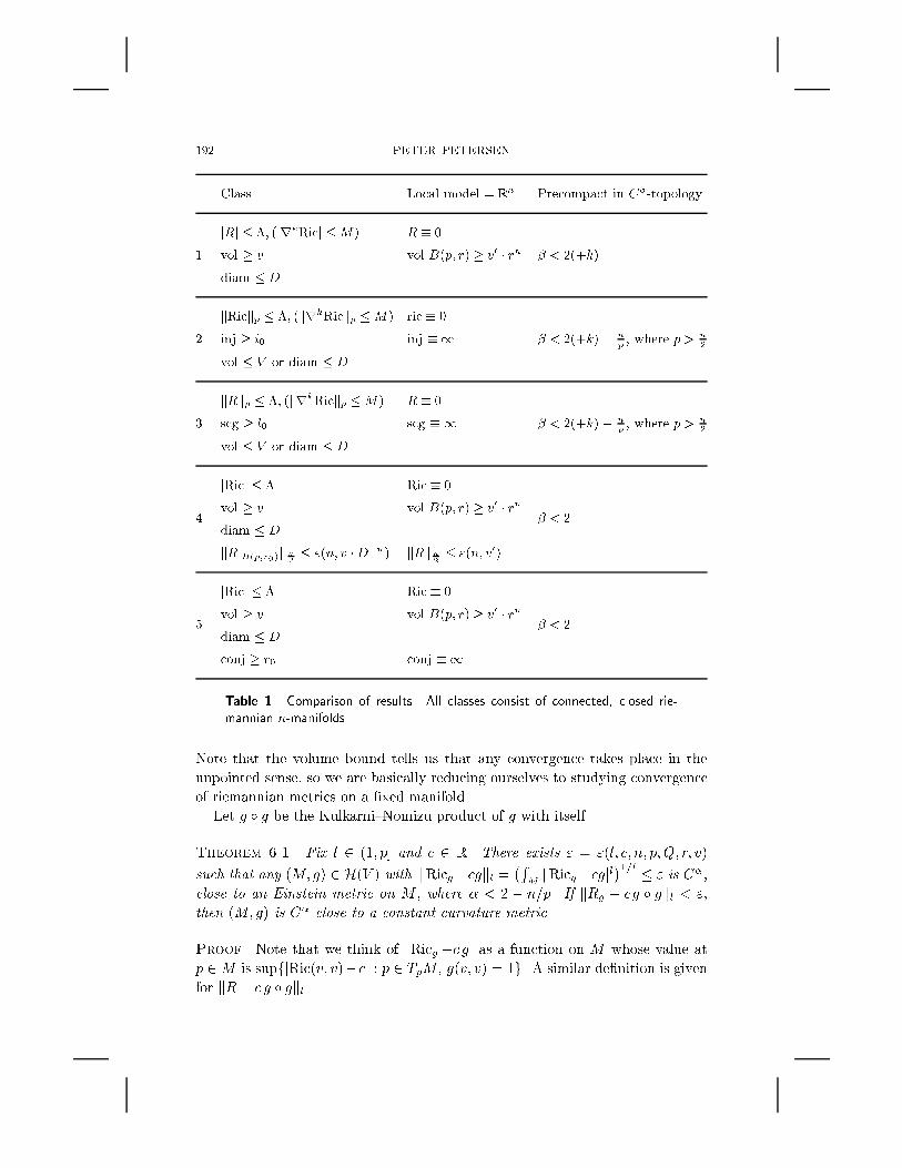
As a �nale, Table 1 lists schematically some of the results we have proved.
6. Applications of Convergence Theory to Pinching Problems
In this section we will present some pinching results inspired by the work
in [Gao 1990]. Our results are more general and the proofs rely only on the
convergence results and their proofs given in previous sections, not on the work
in [Gao 1990].
For p > n=2 � 1 and Q; r > 0, we have the class H(n; p;Q; r) of pointedC1 riemannian n-manifolds with k � kp;2;r � Q. We will be concerned with the
subclass H(V ) = H(n; p;Q; r; V ) of compact manifolds that in addition have
volume at most V . If p > n we know that H(V ) is precompact in the C1+�
topology, for � < 1 � n=p, while if n=2 < p < n the class H(V ) is precompactin both the C� and L1;q, topologies, for � < 2 � n=p and 1=q > 1=p � 1=n.
192 PETER PETERSEN
Class Local model = Rn Precompact in C�-topology
jRj � �; (jrkRicj �M) R � 0
1 vol � v vol B(p; r)� v0 � rn � < 2(+k)
diam � D
kRickp � �; (krkRickp �M) ric � 0
2 inj � i0 inj �1 � < 2(+k)� np, where p > n
2
vol � V or diam � D
kRkp � �; (krkRickp �M) R � 0
3 scg � l0 scg �1 � < 2(+k)� np, where p > n
2
vol � V or diam � D
jRicj � � Ric � 0
4vol � v vol B(p; r)� v0 � rn
� < 2diam � D
kRjB(p;r0)kn2 � "(n; v �D�n) kRkn2� "(n; v0)
jRicj � � Ric � 0
5vol � v vol B(p; r)� v0 � rn
� < 2diam � D
conj � r0 conj �1
Table 1. Comparison of results. All classes consist of connected, closed rie-
mannian n-manifolds.
Note that the volume bound tells us that any convergence takes place in the
unpointed sense, so we are basically reducing ourselves to studying convergence
of riemannian metrics on a �xed manifold.
Let g � g be the Kulkarni{Nomizu product of g with itself.
Theorem 6.1. Fix l 2 (1; p] and c 2 R. There exists " = "(l; c; n; p;Q; r; v)
such that any (M; g) 2 H(V ) with kRicg �cgkl =�R
M jRicg �cgjl�1=l � " is C�,
close to an Einstein metric on M , where � < 2 � n=p. If kRg � cg � gkl < ",
then (M; g) is C� close to a constant curvature metric.
Proof. Note that we think of jRicg �c gj as a function on M whose value at
p 2M is supfjRic(v; v)� cj : p 2 TpM; g(v; v) = 1g. A similar de�nition is given
for kR� c g � gkl.

CONVERGENCE THEOREMS IN RIEMANNIAN GEOMETRY 193
The proof is by contradiction on the existence of such an ". For the sake
of concreteness suppose n=2 < p < n. Using all of our previous work, we can
therefore suppose that we we have a sequence of metrics gi on a �xed manifoldM
such that (M; gi) 2 H(V ) and kRicgi �c gikl converges to 0. We can furthermore
assume that for each i, we have harmonic charts is : B(0; r) ! M , for s =
1; : : : ; N , so that gis�� converges on B(0; r) to some limit riemannian metric gs��in the is�� coordinates. Note that the coordinates vary, but that they will
themselves converge to limit charts s. As in the preliminaries of Theorem 5.1,
we know that the limit coordinates are harmonic.
Now �x s and consider, in the is coordinates, the equation �igi+Q(gi; @gi) =
Ricgi . Here we know that Q(gi; @gi) converges to Q(g; @g) in Lq=2 where 1=q >
1=p � 1=n, and g is the limit metric. Moreover, kRicgi �c gikl ! 0. So we
can conclude that, in the limit harmonic coordinates s, we have the equation
�g+Q(g; @g) = c g or �g = �Q(g; @g)+c g. Here the right-hand side is in Lq=2,with q=2 > p. So we can argue as in the proof of Theorem 5.1 that g is a C1
metric that satis�es the equation �g +Q(g; @g) = c g in harmonic coordinates.
But this implies that the metric is Einstein, which contradicts our assumption
that the gi were not C� close to an Einstein metric.
If we assume that kR� c g � gkl ! 0, we have in particular
kRicg �(n� 1) c gkl ! 0:
So the limit metric is again C1 and Einstein. We will, in addition, have kWkl !0, where W is the Weyl tensor. Since kWkl varies semicontinuously in the C�
topology, the limit space must satisfy kWkl = 0. But then the metric will also
be conformally at, and this makes it a constant curvature metric. �
It is worthwhile pointing out that if we �x c 2 R and assume that kRic�c gkpor kR� c g � gkp is small, where p > n=2, then we have Lp bounds on curvature.
It is, therefore, possible to get some better pinching results in this case. Let's
list some examples.
Theorem 6.2. Let p > n=2 � 1, l; V > 0, and c 2 R be given. There exists " =
"(n; p; l; V; c) such that any (Mn; g) with scg � l, vol � V , and kRg�c g�gkp � "
is Lp;2 close to a constant curvature metric on M .
Proof. The proof, of course, uses Example 5.9 and proceeds as Theorem 1 with
the added �nesse that, since kR � c g � gkp ! 0, we can achieve convergence in
Lp;2 rather than in the weaker C� topology, � < 2� n=p. �
Theorem 6.3. Let p > n=2 � 1, i0; D > 0, and c 2 R be given. There
exists " = "(n; p; i0; D; c) such that any (Mn; g) with inj rad � i0; diam � D and
kRic�c gkp � " is Lp;2 close to an Einstein metric.
Proof. Same as before. �
Finally, we can also improve Gao's result on Ln=2 curvature pinching.
194 PETER PETERSEN
Theorem 6.4. Let n � 2, �; v;D > 0, and c 2 R be given. There exists
" = "(n;�; v;D) such that any (Mn; g) satisfying jRic j � �, vol � v, diam � D,
and kR � c g � gkn=2 � " is C1+� close to a constant curvature metric for any
� < 1.
Proof. Notice that the smallness of kR�c g�gkn=2 implies that kRjB(p;r0)k willbe su�ciently small for some small r. Thus, the class is precompact in the C1+�
topology for any � < 1. We can then use Theorem 6.1 to �nish the proof. �
When dim � 3 we know from Schur's lemma and the identity d Scal = 2 divRic
that pointwise constant sectional curvature implies constant curvature and that
pointwise constant Ricci curvature implies constant Ricci curvature. This can
be used to establish further pinching results, where instead of assuming that the
curvature is close to a constant, we assume smallness of the tensors
R� (n(n� 1))�1 Scal g � g
or Ric�n�1 Scal g. With the background we have established so far, it is not
hard to �nd the appropriate pinching theorems. Further details are left to the
energetic reader.
Appendix A:
Useful Results from [Gilbarg and Trudinger 1983]
Fix a nice bounded domain � Rn , n � 2. For f 2 C1() and 0 < � � 1,
de�ne
kfkk+�;= max
�supx2
j@jf(x)j : jjj � k
�+max
�supx;y2
j@jf(x)� @jf(y)jjx� yj� : jjj = k
�:
Since we don't allow � = 0, there should be no ambiguity about what kfkk+1
is. Also de�ne
kfkp;k; =X
0�jjj�k
�Z
j@jf(x)jpdx�1=p
:
Then de�ne Ck+�() and Lp;k() as the completions of C1() with respect to
the norms k � kk+�; and k � kp;k;, respectively.Sobolev embeddings. Any closed and bounded subset of Lp;k is compact with
respect to the weaker norms k � kl+� (or k � kq;l) provided l + � < k � n=p (or
l < k and 1=q > 1=p� (k � l)=n). In other words, we have compact inclusions
Cl+� � Lp;k for l+� < k�n=p and Lq;l � Lp;k for l < k and 1=q > 1=p�(k�l)=n.
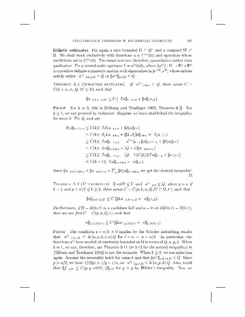
CONVERGENCE THEOREMS IN RIEMANNIAN GEOMETRY 195
Elliptic estimates. Fix again a nice bounded � Rn and a compact 0 ��. We shall work exclusively with functions u 2 C1() and operators whose
coe�cients are in C1(). The issues here are, therefore, quantitative rather than
qualitative. Fix a second-order operator L = aij@i@j , where faijg : ! Rn�Rnis a positive de�nite symmetric matrix with eigenvalues in [e�Q; eQ] whose entries
satisfy either kaijkk+�; � Q or kaijkp;l; � Q.
Theorem A.1 (Schauder estimates). If kaijkk+� � Q, there exists C =
C(k + �; n; Q; 0 � ) such that
kukk+2+�;0 � C�kLukk+�; + kukC0;
�:
Proof. For k = 0, this is [Gilbarg and Trudinger 1983, Theorem 6.2]. For
k � 1, we can proceed by induction. Suppose we have established the inequality
for some k. Fix @j and use
k@jukk+2+� � C(k)(kL@jukk+� + k@jukC0)
� C(k)(k@jLukk+� + k[L; @j ]akk+� + k@jukC0)
� C(k)(kLukk+1+� + kalmkk+�kukk+2+� + k@jukC0)
� C(k)(kLukk+1+� + (Q+ 1)kukk+2+�)
� C(k)(kLukk+1+� + (Q+ 1)C(k)(kLukk+� + kukC0))
� C(k + 1)(kLukk+1+� + kukC0):
Since kukk+1+2+� � kukk+2+� +P
j k@jukk+2+�, we get the desired inequality.
�
Theorem A.2 (Lp estimates). If vol � V and kaijkp;k � Q, where p > n if
k = 1 and p > n=2 if k � 2, there exists C = C(p; k; n;Q;0 � ; V ) such that
kukp;k+1;0 � C (kLukp;k�1; + kukLp;) :
Furthermore, if = B(0; r) is a euclidean ball and u = 0 on @B(0; r) = S(0; r),
then we can �nd C = C(p; n;Q; r) such that
kukp;2;B(0;r) � C (kLukp;B(0;r) + kukp;B(0;r)):
Proof. The condition p � n=k > 0 implies by the Sobolev imbedding results
that kaijkl+�; � K(n; p; k; l; �)Q for l + � < p � n=k. In particular, the
functions aij have moduli of continuity bounded on in terms ofQ;n; p; k. When
k = 1, we can, therefore, use Theorem 9.11 (or 9.13 for the second inequality) in
[Gilbarg and Trudinger 1983] to get the estimate. When k � 2, we use induction
again. Assume the inequality holds for some k and that kaijkp;k+1; � Q. Since
p > n=2, we have 1=(2p) > 1=q � 1=n, so kaijk2p;k; � K(n; p; k)Q. Also, recall
that kfkp; � C(p; q; vol)kfkq; for q > p by H�older's inequality. Now we
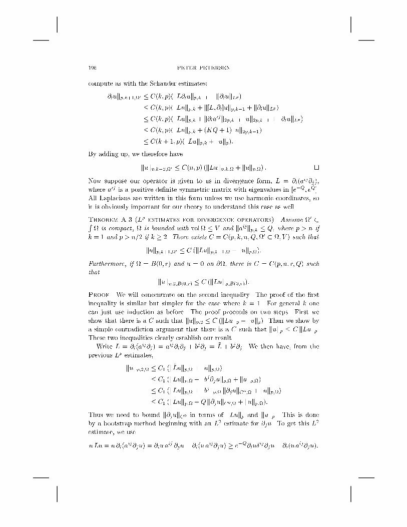
196 PETER PETERSEN
compute as with the Schauder estimates:
k@lukp;k+1;0 � C(k; p)(kL@lukp;k�1 + k@lukLp)� C(k; p)(kLukp;k + k[L; @l]ukp;k�1 + k@lukLp)� C(k; p)(kLukp;k + k@laijk2p;k�1 kuk2p;k�1 + k@lukLp)� C(k; p)(kLukp;k + (KQ+ 1)kuk2p;k�1)
� C(k + 1; p)(kLukp;k + kukp):By adding up, we therefore have
kukp;k+2;0 � C(n; p) (kLukp;k; + kukp;) : �
Now suppose our operator is given to us in divergence form, L = @i(aij@j),
where aij is a positive de�nite symmetric matrix with eigenvalues in [e�Q; eQ].
All Laplacians are written in this form unless we use harmonic coordinates, so
it is obviously important for our theory to understand this case as well.
Theorem A.3 (Lp estimates for divergence operators). Assume 0 �R is compact , is bounded with vol � V and kaijkp;k � Q, where p > n if
k = 1 and p > n=2 if k � 2. There exists C = C(p; k; n;Q;0 � ; V ) such that
kukp;k+1;0 � C (kLukp;k�1; + kukp;):Furthermore, if = B(0; r) and u = 0 on @, there is C = C(p; n; r;Q) such
that
kukp;2;B(0;r) � C (kLukp;B(0;r)):
Proof. We will concentrate on the second inequality. The proof of the �rst
inequality is similar but simpler for the case where k = 1. For general k one
can just use induction as before. The proof proceeds on two steps. First we
show that there is a C such that kukp;2 � C (kLukp + kukp). Then we show by
a simple contradiction argument that there is a C such that kukp � C kLukp.These two inequalities clearly establish our result.
Write L = @i(aij@j) = aij@i@j + bj@j = ~L + bj@j . We then have, from the
previous Lp estimates,
kukp;2; � C1 (k~Lukp; + kukp;)� C1 (kLukp; + kbj@jukp; + kukp;)� C1 (kLukp; + kbjkp; k@jukC0; + kukp;)� C1 (kLukp; +Q k@jukC0; + kukp;):
Thus we need to bound k@jukC0 in terms of kLukp and kukp. This is done
by a bootstrap method beginning with an L2 estimate for @ju. To get this L2
estimate, we use
uLu = u @i(aij@ju) = @iu a
ij @ju� @i(u aij@ju) � e�Q@iu�
ij@ju� @i(u aij@ju):
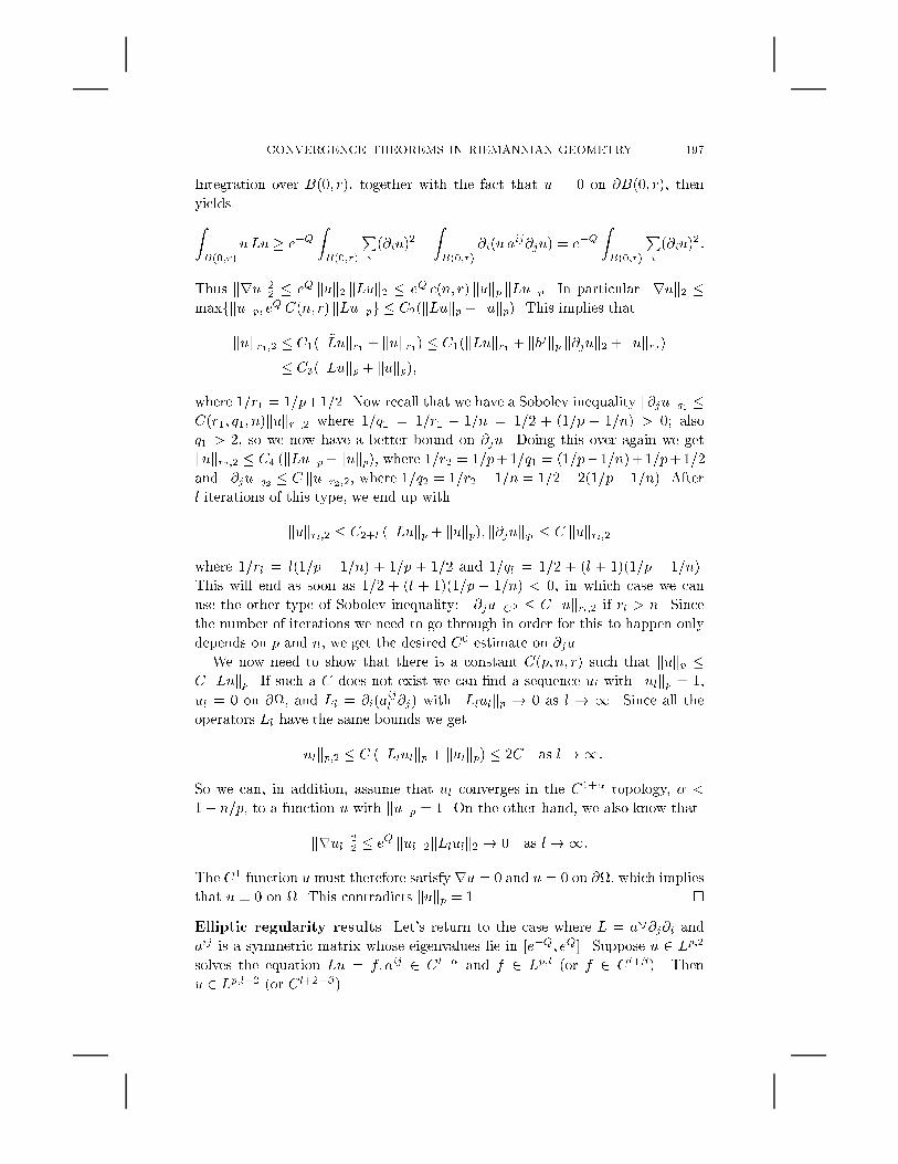
CONVERGENCE THEOREMS IN RIEMANNIAN GEOMETRY 197
Integration over B(0; r), together with the fact that u = 0 on @B(0; r), then
yieldsZB(0;r)
uLu � e�QZB(0;r)
Pi(@iu)
2 �ZB(0;r)
@i(u aij@ju) = e�Q
ZB(0;r)
Pi(@iu)
2:
Thus kruk22 � eQ kuk2 kLuk2 � eQ c(n; r) kukp kLukp. In particular kruk2 �maxfkukp; eQ C(n; r) kLukpg � C2(kLukp + kukp). This implies that
kukr1;2 � C1(k~Lukr1 + kukr1) � C1(kLukr1 + kbjkp k@juk2 + kukr2)� C3(kLukp + kukp);
where 1=r1 = 1=p+1=2. Now recall that we have a Sobolev inequality k@jukq1 �C(r1; q1; n)kukr1;2 where 1=q1 = 1=r1 � 1=n = 1=2 + (1=p � 1=n) > 0; also
q1 > 2, so we now have a better bound on @ju. Doing this over again we get
kukr2;2 � C4 (kLukp+kukp), where 1=r2 = 1=p+1=q1 = (1=p�1=n)+1=p+1=2
and k@jukq2 � C kukr2;2, where 1=q2 = 1=r2 � 1=n = 1=2 + 2(1=p� 1=n). After
l iterations of this type, we end up with
kukrl;2 � C2+l (kLukp + kukp); k@jukql � C kukrl;2
where 1=rl = l(1=p � 1=n) + 1=p + 1=2 and 1=ql = 1=2 + (l + 1)(1=p � 1=n).
This will end as soon as 1=2 + (l + 1)(1=p � 1=n) < 0, in which case we can
use the other type of Sobolev inequality: k@jukC0 � C kukrl;2 if rl > n. Since
the number of iterations we need to go through in order for this to happen only
depends on p and n, we get the desired C0 estimate on @ju.
We now need to show that there is a constant C(p; n; r) such that kukp �C kLukp. If such a C does not exist we can �nd a sequence ul with kulkp = 1,
ul = 0 on @, and Ll = @i(aijl @j) with kLlulkp ! 0 as l ! 1. Since all the
operators Ll have the same bounds we get
kulkp;2 � C (kLlulkp + kulkp) � 2C as l !1:
So we can, in addition, assume that ul converges in the C1+� topology, � <
1� n=p, to a function u with kukp = 1. On the other hand, we also know that
krulk22 � eQ kulk2kLlulk2 ! 0 as l !1:
The C1 function u must therefore satisfy ru = 0 and u = 0 on @, which implies
that u � 0 on . This contradicts kukp = 1. �
Elliptic regularity results. Let's return to the case where L = aij@j@i and
aij is a symmetric matrix whose eigenvalues lie in [e�Q; eQ]. Suppose u 2 Lp;2
solves the equation Lu = f; aij 2 Cl+� and f 2 Lp;l (or f 2 Cl+�). Then
u 2 Lp;l+2 (or Cl+2+�).
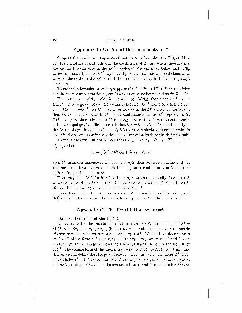
198 PETER PETERSEN
Appendix B: On R and the coe�cients of �
Suppose that we have a sequence of metrics on a �xed domain B(0; r). How
will the curvature operator R and the coe�cients of � vary when these metrics
are assumed to converge in the Lp;k topology? We will show below that kRkpvaries continuously in the Lp;2-topology if p > n=2 and that the coe�cients of �
vary continuously in the Lp-norm if the metrics converge in the Lp;1-topology,
for p > n.
To make the formulation easier, suppose G : � Rn ! Rn �Rn is a positive
de�nite matrix whose entries gij are functions on some bounded domain � Rn .
If we write � = gij@ij + bi@i, bi = @jg
ij + (gij=g)@jg, then clearly gij = G�1
and bi = @jgij+ 1
2gij@j(log g). So we must check howG
�1 and logG depend onG.
Now @iG�1 = �G�1(@iG)G
�1, so if we vary G in the Lp;1-topology, for p > n,
then G, G�1, detG, and detG�1 vary continuously in the C0 topology @iG,
@iG�1 vary continuously in the Lp topology. To see that bi varies continuously
in the Lp topology, it su�ces to check that @jg = @j detG varies continuously in
the Lp topology. But @j detG = F (G; @jG) for some algebraic function which is
linear in the second matrix variable. This observation leads to the desired result.
To check the continuity of R, recall that Rlijk = @i�
ljk � @j�lik +
Pr �
rjk�
lir �
�rik�ljr, where
�ijk =12
Xl
gil(@jgkl + @kglj � @lgjk):
So if G varies continuously in Lp;2, for p > n=2, then @G varies continuously in
L2p; and from the above we conclude that �ijk varies continuously in L1;p � L2p,
so R varies continuously in Lp.
If we vary G in Lp;k, for k � 2 and p > n=2, we can also easily check that R
varies continuously in Lp;k�2, that G�1 varies continuously in Lp;k, and that bi
(�rst order term in �) varies continuously in Lp;k�1.
From the remarks about the coe�cients of �, we see that conditions (h2) and
(h3) imply that we can use the results from Appendix A without further ado.
Appendix C: The Eguchi{Hanson metric
(See also [Petersen and Zhu 1994].)
Let �1; �2 and �3 be the standard left- or right-invariant one-forms on S3 =
SU(2) with d�i = �2�i+1^�i+2 (indices taken modulo 3). The canonical metric
of curvature 1 can be written ds2 = �21 + �22 + �23 . We shall consider metrics
on I � S3 of the form dr2 + '2(r)�21 + 2(r)(�22 + �23), where r 2 I and I is an
interval. We think of ' as being a function adjusting the length of the Hopf �ber
in S3. The volume form of this metric is dr^'(r)�1^ (r)�2^ (r)�3. Using thischoice, we can de�ne the Hodge � operator, which, in particular, maps �2 to �2
and satis�es �2 = 1. The two-forms dr ^'�1 � 2�2 ^�3, dr ^ �2� �3 ^'�1,and dr^ �3�'�1^ �2 have eigenvalues �1 for �, and form a basis for �2TpM
CONVERGENCE THEOREMS IN RIEMANNIAN GEOMETRY 199
for all p 2 M . Normalizing these vectors by 1=p2 we get an orthonormal basis
for �2TpM . In this basis, the curvature operator R has the form�A B
B� D
�;
where A and D are the parts of the curvature tensor on the eigenspaces corre-
sponding to the eigenvalues 1 and �1, respectively. It is a simple algebraic ex-
ercise to see that a four-dimensional manifold is Einstein if and only if sec(�) =
sec(�?) for all planes � and their orthogonal components �?. Using this, one
can check that the metric is Einstein if and only if B � 0. In our case, A, B,
and D are diagonal matrices. If we set Sij = sec(�i ^ �j), where �0 = dr etc.,
and further set M = ( _' � _ ')= 3, the diagonal matrices bemoce
B = 12 diag(�S01 + S23;�S02 + S13;�S03 + S12);
A = 12 diag(S01 + S23 � 4M;S02 + S13 + 2M;S03 + S12 + 2M);
D = 12 diag(S01 + S23 + 4M;S02 + S13 � 2M;S03 + S12 � 2M):
The sectional curvatures can be computed using the tube formula, Gauss equa-
tions, and Codazzi{Maimardi equations, if we think of S3 as sitting in I �S3 as
a hypersurface for each r. We get
S23 =4 2 � 3'2
4�
_ 2
2;
S10 = � �'
';
Sj0 = ��
S1i ='2
4� _' _
'
for j = 2; 3;
for i = 2; 3:
Hence the metric is Einstein if
� �'
'=
4 2 � 3'2
4�
_ 2
2; �
�
='2
4� _' _
' :
One can explicitly solve these equations, but we will only be interested in the
special case where ' = _ and _ 2 = 1�(�=6) 2+k �4, where � is the Einstein
constant and k is just some integration factor. When � = 6 and k = 0, we see
that = sin r and ' = sin r cos r; this corresponds to the Fubini{Study metric
on C P 2. When � = 0 and k < 0, we get a family of Ricci- at metrics. These
are the examples of Eguchi and Hanson. You may want to check that changing
k in this case is the same as scaling the metric.
To get a smooth complete metric, we need the initial condition (0) =
(�k)�1=4. This implies _ (0) = 0, '(0) = 0, and _'(0) = 2. Since _'(0) is
twice as large as we would like, we divide out by the antipodal maps on S3,
which is still an isometry of dr2 + '2�21 + '2(�22 + �23). Then our metric lives
on I � RP3 = I � SO(3), and the Hopf �ber now has length � rather than 2�.
As r ! 0, we can then check that the above metric de�nes a smooth metric on
TS2 =�[0;1) � RP3
�=(0 � RP3), where 0 � RP3 � S2 by the Hopf �bration.

200 PETER PETERSEN
The level set r = 0 is a totally geodesic S2 of constant curvature 4(�k)1=2, whilethe level sets r = r0 are SO(3) with the metric '2(r0)�
21 + 2(r0)(�
22 + �23).
The di�erential equation _ 2 = 1 + k �4 shows that is on the order of r as
r !1. Thus _ ' 1, � = �4k �5 ' 0 as r !1. Using this, one can easily see
that the norm of the curvature operator, jRj, is of order r�6 at in�nity.
The volume form satis�es
dr ^ '(r)�1 ^ 2(r)�2 ^ �3 = 3 (1 + k �4)1=2 dr ^ �1 ^ �2 ^ �3' r3 dr ^ �1 ^ �2 ^ �3:
Thus the metric at 1 is very close to the cone over RP3, namely dr2 + r2(�21 +
�22+�3) on [0;1)�SO(3). This implies that volB(p; r) � 12!4r
4 for all r and p.
Also, kRkp =R jRjp d vol � C
R11 r�3pr3dr = C
R11 r3�3pdr < 1 for p > 4
3 .
In particular, kRkn=2 = kRk2 is �nite.As k ! �1, the level set r = 0 will degenerate to a point and the whole
metric converges to the cone metric dr2 + r2(�21 + �22 + �23) on [0;1) � SO(3).
At the same time, kRk2 stays bounded, but will go to zero on sets r � " > 0.
What happends is that the collapse of S2 absorbs all of the kRk2.We have now constructed some interesting complete Ricci- at metrics. To
get compact examples, we can just use the fact that these examples as k ! �1look like cones, and then glue them into compact examples which locally have
such cones. We illustrate this as done in [Anderson 1990a]: The graphs for '
and look approximately like r at 1. The larger k is, the faster they get to
look linear. For large k, take '; on [0, 5] and then bend them to have zero
derivatives at r = 5. This can be done keeping Ric � 0 and without changing
the volume much. Next re ect ' and in the line r = 5. This yields metrics on
TS2 [ TS2 = S2 �S2 that, near r = 0 and r = 10, look like the Eguchi{Hanson
metric, and otherwise don't change much. As k ! �1, these compact examples
degenerate at r = 0; 10 and the space in the limit becomes a suspension over RP3.
One can see that this process can happen through metrics with 0 � Ric � 1000,
vol � 15 , diam � 10, and kRk2 � 1000.
Acknowledgements
The author would like to thank M. Cassorla, X. Dai, R. Greene, K. Grove,
S. Shteingold, G. Wei and S.-H. Zhu for many helpful discussions on the subject
matter presented here. In addition, I would like to extend special thanks to M.
Christ and S.-Y. Cheng for helping me getting a �rm grip on elliptic regularity
theory and proving the results in Appendix A. Finally, many thanks are due
MSRI and its sta� for their support and hospitality during my stay there.
CONVERGENCE THEOREMS IN RIEMANNIAN GEOMETRY 201
References
[Anderson 1990a] M. T. Anderson, \Short geodesics and gravitational instantons", J.Di�. Geom. 31 (1990), 265{275.
[Anderson 1990b] M. T. Anderson, \Convergence and rigidity of manifolds under Riccicurvature bounds", Invent. Math. 102 (1990), 429{445.
[Anderson 1991] M. T. Anderson, \Remarks on the compactness of isospectral set inlow dimensions", Duke Math. J. 63 (1991), 699{711.
[Anderson 1993] M. Anderson, \Degenerations of metrics with bounded curvature andapplications to critical metrics of Riemannian functionals", pp. 53{79 in Di�erential
geometry: Riemannian geometry (Los Angeles, 1990), edited by R. Greene and S.T. Yau, Proc. Symp. Pure Math. 54, AMS, Providence, RI, 1993.
[Anderson and Cheeger 1991] M. Anderson and J. Cheeger, \Di�eomorphism �niteness
for manifolds with Ricci curvature and Ln=2 norm of curvature bounded", Geom.
Funct. Anal. 1 (1991), 231{252.
[Anderson and Cheeger 1992] M. Anderson and J. Cheeger, \C� compactness formanifolds with Ricci curvature and injectivity radius bounded from below", J. Di�.Geom. 35 (1992), 265{281.
[Bando et al. 1989] S. Bando, A. Kasue, and H. Nakajima, \On a construction ofcoordinates at in�nity on manifolds with fast curvature decay and maximal volumegrowth", Invent. Math. 97 (1989), 313{349.
[Cheeger 1970] J. Cheeger, \Finiteness theorems for Riemannian manifolds", Am. J.
Math. 92 (1970), 61{74.
[Cheeger et al. 1992] J. Cheeger, K. Fukaya, and M. Gromov, \Nilpotent structures andinvariant metrics on collapsed manifolds", J. Amer. Math. Soc. 5 (1992), 327{372.
[Cheeger et al. 1982] J. Cheeger, M. Gromov, and M. Taylor, \Finite propagationspeed, kernel estimates for functions of the Laplace operator, and the geometry ofcomplete Riemannian manifolds", J. Di�. Geom. 17 (1982), 15{53.
[DeTurck and Kazdan 1981] D. M. DeTurck and J. L. Kazdan, \Some regularity
theorems in Riemannian geometry", Ann. Sci. �Ecole Norm. Sup. (4) 14 (1981),249{260.
[Edwards and Kirby 1971] R. Edwards and R. Kirby, \Deformations of spaces ofimbeddings", Ann. Math. (2) 93 (1971), 63{88.
[Fukaya 1990] K. Fukaya, \Hausdor� convergence of riemannian manifolds, and itsapplications", pp. 143{238 in Recent topics in di�erential and analytic geometry,edited by T. Ochiai, Adv. Stud. Pure Math. 18-I, Kinokuniya, Tokyo, and AcademicPress, Boston, 1990.
[Gao 1990] L. Gao, \Convergence of riemannian manifolds: Ricci and Ln=2 curvaturepinching, J. Di�. Geo. 32 (1990), 349{381.
[Gilbarg and Trudinger 1983] D. Gilbarg and N. Trudinger, Elliptic partial di�erentialequations of second order, 2nd ed., Grundlehren der math. Wiss. 224, Springer,Berlin, 1983.
[Greene and Wu 1988] R. E. Greene and H. Wu, \Lipschitz convergence of Riemannianmanifolds", Paci�c J. Math. 131 (1988), 119{141.
202 PETER PETERSEN
[Gromov 1981a] M. Gromov, \Groups of polynomial growth and expanding maps",Publ. Math. IHES 53 (1981), 183{215.
[Gromov 1981b] M. Gromov, Structures m�etriques pour les vari�et�es riemanniennes,edited by J. Lafontaine and P. Pansu, CEDIC, Paris, 1981.
[Jost and Karcher 1982] J. Jost and H. Karcher, \Geometrische methoder zurGewinnung von a-priori-Schranken f�ur harmonische Abbildungen", Manuscripta
Math. 40 (1982), 27{77.
[Karcher 1989] H. Karcher, \Riemannian comparison constructions", pp. 170{222 inGlobal di�erential geometry, edited by S.-S. Chern, MAA Stud. Math. 27, Math.Assoc. America, Washington, DC, 1989.
[Peters 1987] S. Peters, \Convergence of Riemannian manifolds", Comp. Math. 62
(1987), 3{16.
[Petersen 1993] P. Petersen, \Gromov{Hausdor� convergence of metric spaces",pp. 489{504 in Di�erential geometry: Riemannian geometry (Los Angeles, 1990),edited by R. Greene and S. T. Yau, Proc. Symp. Pure Math. 54 (3), Amer. Math.Soc., Providence, 1993.
[Petersen and Zhu 1994] P. Petersen and S.-H. Zhu, \U(2)-invariant four dimensionalEinstein manifolds", preprint, Dartmouth University, 1994.
[Yang 1992] D. Yang, \Convergence of Riemannian manifolds with integral bounds on
curvature I", Ann. Sci. �Ecole Norm. Sup. 25 (1992), 77{105.
Peter Petersen
Department of Mathematics
University of California
Los Angeles, CA 90095