Comparing Visual and Statistical Analysis in Single ...

University of Rhode Island University of Rhode Island

DigitalCommons@URI DigitalCommons@URI

Open Access Dissertations

2013

Comparing Visual and Statistical Analysis in Single-Subject Comparing Visual and Statistical Analysis in Single-Subject

Studies Studies

Magdalena A. Harrington University of Rhode Island, [email protected]

Follow this and additional works at: https://digitalcommons.uri.edu/oa_diss

Recommended Citation Recommended Citation Harrington, Magdalena A., "Comparing Visual and Statistical Analysis in Single-Subject Studies" (2013). Open Access Dissertations. Paper 5. https://digitalcommons.uri.edu/oa_diss/5

This Dissertation is brought to you for free and open access by DigitalCommons@URI. It has been accepted for inclusion in Open Access Dissertations by an authorized administrator of DigitalCommons@URI. For more information, please contact [email protected].

https://digitalcommons.uri.edu/

https://digitalcommons.uri.edu/oa_diss

https://digitalcommons.uri.edu/oa_diss?utm_source=digitalcommons.uri.edu%2Foa_diss%2F5&utm_medium=PDF&utm_campaign=PDFCoverPages

https://digitalcommons.uri.edu/oa_diss/5?utm_source=digitalcommons.uri.edu%2Foa_diss%2F5&utm_medium=PDF&utm_campaign=PDFCoverPages

mailto:[email protected]

COMPARING VISUAL AND STATISTICAL ANALYSIS

IN SINGLE-SUBJECT STUDIES

BY

MAGDALENA A. HARRINGTON

A DISSERTATION SUBMITTED IN PARTIAL FULFILLMENT OF THE

REQUIREMENTS FOR THE DEGREE OF

DOCTOR OF PHILOSOPHY

IN

PSYCHOLOGY

UNIVERSITY OF RHODE ISLAND

2013

DOCTOR OF PHILOSOPHY DISSERTATION

OF

MAGDALENA A. HARRINGTON

APPROVED:

Dissertation Committee:

Major Professor Wayne F. Velicer, PhD

Colleen Redding, PhD

Bryan Blissmer, PhD

Nasser H. Zawia

DEAN OF THE GRADUATE SCHOOL

UNIVERSITY OF RHODE ISLAND

2013

ABSTRACT

Objective. There has been an ongoing scientific debate regarding the most

reliable and valid method of single-subject data evaluation in the applied behavior

analysis area among the advocates of the visual analysis and proponents of the

interrupted time-series analysis (ITSA). To address this debate, a head-to-head

comparison of both methods was performed, as well as an overview of serial

dependency, effect sizes and sample sizes.

Method. The comparison of both methods was conducted in two independent

studies. In the first study, conclusions drawn from visual analysis of the graphs

published in the Journal of Applied Behavior Analysis (2010) were compared with the

findings based on the ITSA of the same data; in the second study, conclusions drawn

from visual analysis of the graphs obtained from the textbook by Alan E. Kazdin

(2011) were used. These comparisons were made possible by the development of

software, called UnGraph®

which permits the recovery of the raw data from the

graphs, allowing the application of ITSA.

Results. In both studies, ITSA was successfully applied to over 90% of the

examined time-series data with numbers of observations ranging from 8 to 136. Over

60% of the data had moderate to high level first order autocorrelations (> .40). A large

effects size (≥ .80) was found for over 70% of eligible studies. Comparison of the

conclusions drawn from visual analysis and ITSA revealed an overall low level of

agreement (Kappa = .14) in the first study and moderate level of agreement (Kappa =

.44) in the second study.

Conclusions. These findings show that ITSA can be broadly implemented in

applied behavior analysis research and can facilitate evaluation of the intervention

effect, particularly when specific characteristics of single-subject data limit the

reliability and validity of visual analysis. Comparison of the two methods revealed low

to moderate agreement between visual analysis and ITSA. Overall, the two methods

should be viewed as complimentary and used concurrently.

iv

ACKNOWLEDGMENTS

I would like to thank my Major Professor, mentor and an outstanding teacher

Wayne Velicer, for his support and guidance throughout my graduate school career.

His contribution to this dissertation has been invaluable. I also want to acknowledge

and thank my committee members. I would also like to thank Janette Baird, for

introducing me to statistics and SAS, and for her ongoing support, advice, and

encouragement. Finally, special thanks to my son, Alexander, for his patience.

v

DEDICATION

To Alexander

vi

PREFACE

This dissertation addresses the scientific debate regarding the most reliable and

valid method of single-subject data evaluation in the applied behavior analysis

research field. The primary emphasis is placed on the head-to-head comparison of the

conclusions based on visual analysis and interrupted-times series analysis (ITSA) of

the same single-subject data.

This dissertation consists of two independent studies, each presented in the

manuscript format prepared for submission for publication in a peer reviewed journal.

The first chapter of the dissertation provides an introduction and overview of the

topic.

The second chapter presents the first study that compares the visual analysis of

graphical data and ITSA published in the Journal of Applied Behavior Analysis

(2010).

The third chapter presents the second study that compares the visual analysis of

the graphical data and ITSA obtained from the book titled “Single-Case research

designs: Methods for clinical and applied settings” by Alan E. Kazdin (2011).

The fourth chapter provides the comparison of findings obtained from each study

and final conclusions.

vii

TABLE OF CONTENTS

ABSTRACT .................................................................................................................. ii

ACKNOWLEDGMENTS .......................................................................................... iv

DEDICATION .............................................................................................................. v

PREFACE .................................................................................................................... vi

TABLE OF CONTENTS........................................................................................... vii

LIST OF TABLES .................................................................................................... viii

LIST OF FIGURES .................................................................................................... ix

CHAPTER 1 ................................................................................................................. 1

INTRODUCTION ........................................................................................................ 1

CHAPTER 2 ................................................................................................................. 4

Comparing Visual and Statistical Analysis in Single-Subject Studies: Results for

Journal of Applied Behavior Analysis Examples ....................................................... 4

CHAPTER 3 ............................................................................................................... 64


Kazdin Textbook Examples ..................................................................................... 64

CHAPTER 4 ............................................................................................................. 114

CONCLUSIONS ...................................................................................................... 114

viii

LIST OF TABLES

TABLE PAGE

Table 1. Summary of the visual analysis and interrupted time-series analysis based on

eligible studies published in the Journal of Applied Behavior Analysis in 2010. ...... 42

Table 2. Summary of the visual analysis and interrupted time-series analysis based on

eligible graphs presented in the “Single-Case Research Designs. Methods for Clinical

and Applied Settings” by A. E. Kazdin (2011) ........................................................... 97

ix

LIST OF FIGURES

FIGURE PAGE

Figure 1. Distribution of Lag-1 Autoregressive Coefficients in Eligible Time Series

Data (K = 163). ........................................................................................................... 56

Figure 2. Distribution of the Cohen’s d Effect Size Estimates for Eligible Time Series

Data (k = 98). .............................................................................................................. 57

Figure 3. Agreement between graphical analysis and statistical analysis .................. 58

Figure 4. Graphical presentation of the data illustrated in the first example of ITSA

application ................................................................................................................... 59


application ................................................................................................................... 60

Figure 6. Graphical presentation of the data illustrated in the second example of ITSA

application ................................................................................................................... 61

Figure 7. Graphical presentation of the data illustrated in the third example of ITSA

application ................................................................................................................... 62


application ................................................................................................................... 63


Data (K = 75). ........................................................................................................... 103


Data (k = 44). ............................................................................................................ 104

Figure 11. Agreement between graphical analysis and statistical analysis .............. 105

x


application ................................................................................................................. 106


application ................................................................................................................. 107

Figure 14. Graphical presentation of the data illustrated in the second example of

ITSA application ....................................................................................................... 108










application ................................................................................................................. 113

1

CHAPTER 1

INTRODUCTION

Currently, there are two widely used methods for evaluating intervention effects

based on single-subject research designs. Visual analysis of graphs presenting

experimental data is a commonly used approach in applied behavior analysis research,

while interrupted time-series analysis (ITSA) is a statistical method used in research

fields, such as electrical engineering, economics, business, and other areas of

psychology, to name just a few. The use of visual analysis preceded the development

of quantitative methods like time series analysis which required high speed computers

to implement.

There has been an ongoing scientific debate regarding the most reliable and valid

method of single-subject data evaluation in the applied behavior analysis area among

the advocates of visual analysis and the proponents of interrupted time-series analysis

(ITSA).

Visual analysis, although guided by a set of criteria, is mostly driven by a

subjective evaluation of intervention effects. Advocates of this approach state that

large intervention effects are evident and provide unequivocal conclusions easily

observed by independent judges. It is argued that the rationale for using visual analysis

is to highlight large (i.e. easily observable) intervention effects and disregard small

(i.e. not easily observable) effects, concluding that visually undetected intervention

effects have insignificant clinical impact. Proponents of visual analysis state that the

2

conservative approach to evaluating intervention effects guarantees highly accurate

and consistent conclusions across independent judges, as well as reduces unknown

probability of Type I error rate and consequently increases the probability of Type II

error rate.

Several studies examined agreement rates among judges and showed that visual

analysis led to inconsistent conclusions about intervention effects across different

raters and that the inter-rater agreement among judges who reviewed the same graphs

was relatively poor, suggesting that visual analysis is not a reliable method for

assessing intervention effects of single-subject data. Factors such as high complexity

of the data and experimental design, high variability of the data, changes in slope, and

serial dependency of the single-subject data were associated with lower agreement

rates among judges and increased Type I error rates.

On the other hand, advocates of the visual analysis call attention to some

drawbacks of ITSA, such as difficulty to accurately estimate ARIMA model,

requirement of a large number of observations, and inability to apply this statistical

method to complex single-subject experimental designs.

To address this debate, a head-to-head comparison of both methods was

performed in two independent studies.

The first study used the graphical data based on the single-subject studies

published in the Journal of Applied Behavior Analysis (2010). The journal was

selected because it is a leading journal on the topic used by applied researcher and it

strongly promotes the use of visual analysis rather than statistical methods.

3

In the second study, graphical data was obtained from the book titled “Single-

Case research designs: Methods for clinical and applied settings” by Alan E. Kazdin

(2011), who is currently the leading advocate of visual analysis of single-subject

studies. The book is a widely used textbook within applied psychology area and

provides numerous examples of graphs presenting single-subject experimental data

with corresponding evaluations of intervention effects based on visual analysis.

4

CHAPTER 2


Journal of Applied Behavior Analysis Examples

Manuscript submitted to Psychological Methods, March 2013

5

Abstract



analysis area among the advocates of the visual analysis and proponents of the

interrupted time-series analysis (ITSA). To address this debate, a head-to-head

comparison of both methods was performed, as well as an overview of serial

dependency, effect sizes and sample sizes.

Method. Conclusions drawn from visual analysis of the graphs published in the

Journal of Applied Behavior Analysis (2010) were compared with the findings based

on the ITSA of the same data. This comparison was made possible by the development

of software, called UnGraph®

which permits the recovery of the raw data from the

graphs, allowing application of ITSA.

Results. ITSA was successfully applied to 94% of the examined time-series data

with number of observations ranging from 8 to 136. Over 60% of the data had

moderate to high level first order autocorrelations (> .40). A large effect size (≥ .80)

was found for 73% of eligible studies. Comparison of the conclusions drawn from

visual analysis and ITSA revealed an overall low level of agreement (Kappa = .14).


applied behavior analysis research and can facilitate evaluation of intervention effects,

particularly when specific characteristics of single-subject data limit the reliability and

validity of visual analysis. These two methods should be viewed as complimentary

and used concurrently.

6

Keywords: Applied Behavior Analysis, Single-subject Studies, Visual Analysis,

Interrupted Time-series Analysis, Effect Size, Serial Dependency

7


Journal of Applied Behavior Analysis Examples

Group-level and single-subject research designs are two methodological models

employed for analyzing longitudinal research. The first model is based on data

obtained from a large number of individuals and provides average estimates of

longitudinal trajectories of behavior change based on group-level data, emphasizing

between-subject variability. A significant limitation of group-level designs, also

known as nomothetic designs, is the inability to capture high levels of variability and

heterogeneity within the studied populations (Molenaar, 2004). Further, group-level

designs emphasize central tendencies of the population and consequently obscure

natural patterns of behavior change, their multidimensionality and unique variability

within each individual (Molenaar & Campbell, 2009).

The second methodological approach employed in longitudinal research is based

on data obtained from one individual or unit (n = 1) through intensive data collection

over time. Single-subject designs, also known as idiographic designs, examine

individual-level data, that allows for highly accurate estimates of within-subject

variability and longitudinal trajectories of each individual’s behavior. Idiographic

methodology characterizes highly heterogeneous processes, which consequently allow

for more accurate inferences about the nature of behavior change specific to an

individual (Velicer & Molenaar, 2013). Single-subject designs address the limitations

of group-level designs and present several advantages. They allow for a highly

accurate assessment of the impact of the intervention for each individual while group-

8

level designs provide information about the effectiveness of the intervention for an

“average” person, rather than any person in particular (Velicer & Molenaar, 2013).

In addition, single-subject research allows studying longitudinal processes of

change with much better precision than group-level designs, due to a higher number of

data points and better controlled variability of the data. Also, it can be applied to

populations that are otherwise difficult to recruit in numbers large enough to allow for

a group-level design (Barlow, Nock, & Hersen, 2009; Kazdin, 2011).

Methods of evaluating single-subject studies


based on single-subject designs. Visual analysis of the graphs presenting experimental

data is a commonly used approach in applied behavior analysis research, while

interrupted time-series analysis (ITSA) is a statistical method used in research fields,

such as electrical engineering, economics, business, and other areas of psychology, to

name just a few. The use of visual analysis preceded the development of quantitative

methods like time series analysis which required high speed computers to implement.

Visual analysis

The most basic experimental model used in single-subject research is an A-B

design with a well defined target behavior that is examined before and after the

intervention. The first phase (A) of the design consists of multiple baseline

observations that assess the pre-intervention characteristics of the behavior. In the

second phase (B) of the design, the treatment component of the experiment is

introduced and changes in behavior are examined (Barlow et al., 2009; Kazdin, 2011).

9

The visual analysis of the graph, performed by a judge or a rater, is based on a set

of criteria that evaluate and compare the characteristics of phase A and B and examine

whether behavior changes in phase B are a result of the intervention. The baseline (A)

phase provides information about the descriptive and predictive aspects of the target

behavior, such as stability and variability. Stable behavior, characterized by the

absence of a trend or slope in the data, indicates that the targeted behavior neither

increases nor decreases on average over time during the baseline phase (Kazdin,

2011). Variability of the data is characterized by the changes in the behavior within

the range of possible low and high levels (Barlow et al., 2009). Single-subject

experiments are evaluated based on magnitude and rate of change between phase A

and B. The magnitude of change is based on variability in level and slope of the data.

Changes in level refer to average changes in the frequency of target behavior, whereas

changes in slope refer to shifts in direction of the behavior across different phases. The

mean is the average for all data in a particular phase. If the series is stable, the level

will equal the slope. Changes in level and slope are independent from each other. Rate

of change is based on changes in trend or slope of the data and latency of change.

Trend analysis provides information on systematic increases or decreases in the

behavior across phases, whereas latency of change refers to the amount of time

between the termination of one phase and changes in behavior (Kazdin, 2011).

Visual analysis, although guided by the set of criteria described above, is not

based on any specific decision making rules and it is mostly driven by subjective

evaluation of the intervention effects. Advocates of this approach argue that large

intervention effects are evident and provide unequivocal conclusions that can be easily

10

observed by independent judges. Further, it is argued that the subjective evaluation of

intervention effects has a minimal impact on reliability and validity of the conclusions

drawn from the graphs presenting large and therefore easily observable treatment

effects, since only those are considered to have significant clinical implications (Baer,

1977; Kazdin, 2011). This concept is particularly promoted in the field of applied

behavior analysis.

Proponents of visual analysis acknowledge that certain characteristics of single-

subject data can significantly impair the ability to accurately evaluate intervention

effects. The presence of slope in the baseline phase of the experiment may negatively

affect the evaluation of the experiment, especially when the trend of the targeted

behavior is moving in the same direction as would be expected due to treatment

effects. High variability of the data may also interfere with the validity of the

conclusions. For example, accuracy of the evaluation of intervention effects on

disruptive behavior can be significantly affected by a pattern of behavior that is

decreasing (getting better) over time. Also high variability of the behavior, such as

extreme fluctuations from none to high frequency of disruptive behavior can limit the

ability to draw valid conclusions about intervention effects (Kazdin, 2011). However,

it is argued that the rationale for using visual analysis is to highlight large (i.e. easily

observable) intervention effects and disregard small (i.e. not easily observable) effects.

It is concluded that visually undetected intervention effects have insignificant clinical

impact. Proponents of visual analysis state that the conservative approach to

evaluating intervention effects guarantees highly accurate and consistent conclusions

across independent judges, as well as reduces unknown probability of Type I error rate

11

and consequently increases the probability of Type II error rate (Baer, 1977; Kazdin,

2011).

In the recent literature, some of the visual analysis advocates have discussed the

problem of the lack of effect size estimation which results in an inability to perform

meta-analytic reviews single-subject experiments. As stated by Kazdin (2011), the

single-subject research field would benefit from the ability to integrate a large number

of studies in a systematic way that would allow drawing broader conclusions

regarding intervention effects that would generalize beyond single experiments.

However, to date there is no consensus regarding guidelines for interpreting effect

sizes calculated based on supplementing visual analysis methods commonly used

among single-case researchers. Brossart, Parker, Olson, and Mahadevan (2006)

compared five analytic techniques frequently used in single-subject research applied to

the same data and concluded that each analytical approach was strongly influenced by

serial dependency, and the obtained results based on each method varied so much that

it prohibited the development of any reliable effect-size interpretation guidelines.

Inability to estimate effect sizes based on currently used analytical methods leaves

meta-analytic approaches out of reach in the field of single-subject research. A

noteworthy study by Hedges, Pustejovsky and Shadish (2012) proposed new effect

size that is comparable to Cohen’s d, frequently used in group-level designs. It is

applied across single-subject cases and it can be used in studies with at least three

independent cases. This new approach can be applied in meta-analytic research and

warrants further examination.

12


analysis led to inconsistent conclusions about the intervention effects across different

raters. The inter-rater agreement among judges who reviewed the same graphs was

relatively poor, ranging on average from .39 to .61 (Jones, Weinrott, & Vaught, 1978;

DeProspero & Cohen, 1979; Ottenbacher, 1990), suggesting that visual analysis is not

a reliable method for assessing intervention effects of single-subject data. Higher

complexity of the data and experimental design resulted in less consistent conclusions.

Factors like high variability of the data, inconsistent patterns of behavior over time,

changes in slope, and small changes in level of the data were associated with lower

agreement rates across judges (DeProsper & Cohen, 1979; Ottenbacher, 1990).

In addition, Matyas and Greenwood (1990) showed that a positive autocorrelation

and high variability in the data tend to increase Type I error rates. These findings

suggest that the claimed advantages of visual analysis resulting in reduced Type I error

rates are overstated.

Several studies demonstrated that higher levels of serial dependency in single-

subject data lead to higher rates of disagreement between visual and statistical analysis

(Bengali & Ottenbacher, 1998; Jones et al., 1978; Matyas & Greenwood, 1990). One

study by Jones et al. (1978) showed that the highest level of agreement between the

two methods was found when there were non-statistically significant changes in the

behavior and the lowest agreement occurred when there were significant effects of the

intervention. These findings suggest that statistically significant results may be more

often overlooked by visual analysis than non-significant results and that the highest

13

agreement between these two methods occurs when there is no serial dependency in

the data and intervention effects are insignificant.

Interrupted time-series analysis

Interrupted time-series analysis (ITSA) is a statistical method used to examine

intervention effects of single-subject study designs. It is based on chronologically

ordered observations obtained from a single subject or unit. An inherent property of

time-series data is serial dependency that reflects the impact of previous observations

on the current observation and violates the assumption of independence of errors,

which can significantly affect the validity of the statistical test. Serial dependency,

examined by the magnitude and direction of autocorrelations between observations

spaced at different time intervals (lags), directly impacts error term estimation and

validity of the statistical test. Negative autocorrelations produce an overestimation of

the error variance, which leads to conservative bias and increases Type II error rate,

whereas positive autocorrelations lead to underestimation of the error variance, and

cause liberal bias and increase Type I error rates (see Velicer & Molenaar, 2013 for an

illustration).

The most widely used model for examining serial dependency in the data is the

autoregressive integrated moving average (ARIMA) model. It consists of three

elements to be evaluated. The autoregressive term (p) estimates the extent to which the

current observation is predictable from preceding observations and the number of past

observations that impact the current observation. The moving average term (q)

estimates the effects of preceding random shocks on current observation. The

integrated term (d) refers to the stationarity of the series. Stationarity of time-series

14

data requires the structure and the parameters of the data, such as mean, variance and

the patterns of the autocorrelations to remain the same across time for the series. Non-

stationary data requires differencing in order to keep the series at a constant mean

level, otherwise reliability of the assessed intervention effects can be compromised

(Glass, Willson, & Gottman, 2008).

The ITSA method is able to measure the degree of the serial dependency in the

data and statistically remove it from the series, allowing for an unbiased estimate of

the changes in level and trend across different phases of the experiment (Glass et al.,

2008). In addition, after accounting for serial dependency in the data, ITSA facilitates

an estimate of Cohen’s d effect size (Cohen, 1988), which is the most commonly used

measure of intervention effects in behavioral sciences research with widely

implemented interpretative guidelines.

ITSA limitations

Although, the most recommended method for removing serial dependency from

single-subject data is implementing an ARIMA model (Glass et al., 2008), some

researchers call attention to some drawbacks of ITSA related to accurate ARIMA

model estimation and limited utility in applied behavior analysis studies (Ottenbacher,

1992; Kazdin, 2011). Identifying the correct ARIMA model has been shown to be

often unreliable, leading to model misidentification (Velicer & Harrop, 1983).

However this issue has been addressed through the general transformation method,

which uses the ARIMA model for lag-5 autocorrelation (5, 0, 0) that was shown to be

simpler and more accurate than other model specification methods (Velicer &

McDonald, 1984). For shorter time-series data a simpler model based on lag-1

15

autocorrelation (1, 0, 0) is sufficient when applied to data that does not require

forecasting (Simonton, 1977). Simulation studies have shown that these procedures

are very accurate (Harrop & Velicer, 1985; Harrop & Velicer, 1990).

Another disadvantage of the ARIMA procedure has been associated with the

requirement of a large number of observations. A minimum of 35-40 observations or

even as high as 25 observations per phase were recommended (Glass et al., 2008;

Ottenbacher, 1992) in order to correctly identify an ARIMA model. However,

application of predetermined ARIMA model allows for reliable evaluation of shorter

data series. In addition, proponents of visual analysis argue that ITSA may not be a

suitable analytical approach for experimental designs that reach beyond the basic AB

model, such as alternating treatment designs or multiple baseline designs (Barlow et

al., 2009; Kazdin, 2011).

Study Aims

This study will perform a head-to-head comparison of the conclusions drawn

from visual analysis of graphically presented data with the findings based on

interrupted time-series analysis of the same data. The study will use graphical data

based on single-subject studies published in the Journal of Applied Behavior Analysis

(2010). This journal was selected because it is a leading journal on the topic used by

applied researchers and it strongly promotes the use of visual analysis rather than

quantitative analysis methods (Shadish & Sullivan, 2011; Smith, 2012). In a related

study, all the studies published in a leading textbook (Kazdin, 2011) were evaluated in

the same way (Harrington & Velicer, 2013).

16

The aim of this study is to examine the level of agreement between these two

methods, as well as degree of serial dependency in single-subject data, and estimate

the effect size for each study. This comparison is made possible by the development of

a statistical program called UnGraph® software version 5.0 (Biosoft, 2004), which

permits the recovery of raw data and the application of interrupted time series

analysis.

Method

Sample

Graphical data was obtained from the research papers published in the Journal of

Applied Behavior Analysis (JABA) in 2010. For a graph to be included in this study,

it was required to meet the following inclusion criteria: (1) present actual data (not

simulated); (2) present interrupted time-series data; (3) present a minimum of three

observations in each phase of the design in order to estimate a full four parameter

model; (4) present baseline and treatment phases of an experimental design; (5)

include corresponding description of the conclusions drawn from the visual analysis of

the graph; and (6) present well defined data points (observations) in the graph. Graphs

presenting cumulative data or alternating-treatment designs were not eligible.

Procedure

Eligible graphs were scanned and electronically imported into UnGraph®

software version 5.0 (Biosoft, 2004). Next, data presented in each graph was extracted

using the UnGraph® software’s function of coordinate system that defined each

17

graph’s structure and scale. Then, sequentially ordered data recorded into a time-series

data format was exported into a Microsoft Excel® spreadsheet.

Validity and reliability of UnGraph®

software

UnGraph® software has been previously examined for its validity and reliability

when extracting data from graphs representing single-case designs (Shadish et al.,

2009). Results of this study indicated high validity and reliability of the extracted data

from graphs, with .96 as an average correlation coefficient between two raters.

Analysis

Interrupted time-series analyses (ITSA) were used to evaluate intervention effects

of each single-subject study based on the data collected using UnGraph® software.

Identification of the ARIMA model was performed in a series of steps. First, level of

autocorrelation in the data was evaluated based on autocorrelation function (ACF) and

partial autocorrelation function (PACF). These two functions refer to autoregressive

and moving average parameters and estimate whether negative or positive correlation

was present in the data series, as well as in how many lags the correlation was present.

Also, the stationarity parameter (d) was evaluated, and if required, differencing of the

data was performed.

Second, values of each parameter were estimated and the fit of the ARIMA model

was evaluated. The best fitting model resulted in uncorrelated residuals. In cases when

the residuals were correlated, the model identification process was repeated and a new

model was evaluated (Barlow et al., 2009; Glass et al., 2008). Once a correctly

identified ARIMA model was applied to single-subject data, parameters such as trend,

18

change in trend, level, change in level, as well as mean and variability of the series

were evaluated. Intervention effects were examined based on changes in slope and

level across the experimental phases of the design. In addition, for studies where no

significant slope or change in slope was present, Cohen’s d effect size was calculated

to examine the magnitude of the behavior change due to the intervention. Analyses

were performed in SAS version 9.2. This study was approved by the University of

Rhode Island Institutional Review Board.

Description of the visual analysis of the graphs presented in the publications

published in JABA was used to perform a head-to-head comparison of the findings

based on each method. These comparisons were based on conclusions made in regards

to trend, change in trend, variability of the data and change in level of the data across

different experimental phases of the experiment.

Results

Sample

A total of 75 research papers were published in the JABA in 2010. After

reviewing the content of the publications, 25 papers met eligibility criteria and were

included in the study. Excluded publications did not present interrupted time-series

data (k = 27), presented less than 3 observations in at least one phase of the design (k

= 4), presented cumulative data (k = 3), or alternating-treatment designs (k = 9). One

study presented generated, hypothetical data, and one study presented a graph with

insufficiently defined observations, which prevented data point extraction. Five studies

were ineligible because the presented description of the findings based on the visual

analysis of the graph was not possible to verify using ITSA.

19

The eligible publications included one or more graphs. A total of 99 graphs

presenting interrupted time-series data with corresponding conclusions based on visual

analysis were included in the study. The graphs displayed a diversified range of

single-subject designs, such as AB design and its variations (e.g. ABA, ABAB), ABC

design and its variations (e.g. ABCA, ABCACA, ABABACBC), and designs that

included more than two different interventions (e.g. ABCD, ABCDEFBFEDC) (see

Table 1 for details).

Each graph presented one or more interrupted time-series data (e.g., data points

presenting two independent behaviors were plotted on one graph). Conclusions based

on visual analysis were applied to either the full study design or to one or more

sections of the design. ITSA was applied to the data with the corresponding

description of the findings formulated in a way that could be validated using statistical

methods. A total of 163 ITSA were performed.

Descriptive statistics

The number of observations in the analyzed experiments ranged from 8 to 136,

with minimum of 3 and maximum of 90 observations per phase. For 9 (5.52%)

analyzed experiments, the interrupted-time series ARIMA model did not converge.

Six of those experiments came from one study that had multiple single-subject data

series characterized by low number of observations (< 12) and low variability across

observations; two experiments had higher number of observations (43 and 136) but

low variability across observations; one experiment had high variability across 22

observations.

20

For the remaining 154 time-series data, 23 (14.94%) had significant slope, 15

(9.74%) had significant change in slope due to experimental design, 18 (11.69%) had

significant slope and change in slope. The nonlinearity of the slopes was not

examined.

Over 50% of the examined time-series data (k = 79) had significant changes in

level due to examined study design phase change.

The general transformation method (Velicer & McDonald, 1984), which uses the

ARIMA (5, 0, 0) model for lag-5 autocorrelation was successfully applied to 32

experiments (20.78%), all of which had 30 or more observations. A simpler ARIMA

model based on lag-1 autocorrelations (1, 0, 0) (Simonton, 1977) was applied to 120

experiments (77.92%). ARIMA models (3, 0, 0) and (2, 0, 0) were applied to two

experiments.

Small lag 1 autocorrelations ranging from .00 to .20 were found for 15 time-series

data, small-medium lag 1 autocorrelations ranging from .21 to .40 were found for 34

time-series data, medium lag 1 autocorrelations ranging from .41 to .60 were found for

61 time-series data, and large lag 1 autocorrelations .61 or larger were found for 40

time-series data. Lag 1 autocorrelation less than .00 were found for 13 time-series data

and ranged from -.32 to -.05. Lag 1 autocorrelations were significant for 93 time-series

data, 28 of those time-series data also had significant lag 2 autocorrelations. The

autocorrelations were not corrected for small sample bias (Shadish & Sullivan, 2011).

Figure 1 presents the distribution of the lag-1 autocorrelations for the eligible studies

and details are presented in Table 1.

21

Cohen’s d effect size was estimated for all experiments that did not have

significant slope or change in slope, a total of 98 (63.64%). The effect sizes ranged

from 0.00 to 22.74. Figure 2 presents the distribution of the effect size estimates for

the eligible studies. Based on Cohen’s (1988) classification, small effect sizes, ranging

from .20 to .49 were found for 8 time-series data, medium effect sizes, ranging from

.50 to .79 were found for 8 time-series data, and large effect sizes of .80 or greater

were found for 72 time-series data (73.47%). Details are provided in Table 1.

ITSA and visual analysis comparison

Comparison of the findings based on visual analysis and ITSA demonstrated

consistent findings for 94 analyzed time-series data. Most of those consistent findings

(k = 79) referred to significant changes between different phases of the experiment,

while 15 referred to non-significant changes such as reversal to baseline. For the

remaining 60 experiments (38.96%), the findings based on statistical analysis did not

confirm the conclusions based on visual analysis (bolded data in Table 1). For 52 of

those experiments, visual analysis indicated significant changes between different

phases of the study design, when statistical analysis did not reveal significant

differences. For 8 experiments, non-significant findings based on visual analysis were

not confirmed by statistical analysis. See Figure 3 for a summary of the agreement and

disagreement between the two methods. The overall level of agreement was low

(Cohen’s Kappa = .14) (Cohen, 1960). Among the experiments that led to inconsistent

findings between the two methods, 30% had significant slope, change in slope or both,

and 53% had lag-1 autoregressive term greater than .40.

22

To illustrate the application of the ITSA method in the analysis of single-subject

studies and comparison with the conclusions drawn on visual analysis, three examples

were selected from the experiments presented in Table 1.

Example 1

The first example is based on a study that examined the effects of providing praise and

preferred edible items based on variable-time schedule in order to reduce problem

behavior. In addition, effects of variable-time schedule on compliance were also

evaluated. The study was based on a reversal design (ABAB) and included three

participants (Lomas, Fisher, & Kelly, 2010). In the current example, data for one of

the participants is provided. Sam was 8 years old boy diagnosed with Asperger

syndrome and attention deficit hyperactivity disorder. Data displaying frequency of

problem behavior and percentage of compliance in each phase of the design is

presented in Figure 4 and Figure 5, respectively. Conclusions based on visual analysis

of the data suggested that the variable-time schedule reduced problem behavior, but

did not increase compliance for Sam. Lomas et al. (2010) stated that “ levels of

compliance were only slightly higher during treatment with VT food and praise for

Sam . . . “ and that “variable-time delivery of food and praise superimposed on a

demand baseline (in which problem behavior continued to produce escape) greatly

reduced problem behavior . . .” (p. 431).

ITSA was implemented to evaluate the effect of variable-time delivery on

problem behavior and compliance. The ARIMA (1, 0, 0) was applied to both

behaviors to estimate 4 parameters: level, change in level, slope and change in slope.

23

For problem behavior, lag 1 autocorrelation was .40. The analysis for slope and

change in slope yielded non-significant findings, whereas change in level in the

variable-time delivery phase indicated significant decrease in problem behavior (t (18)

= -2.39, p < .05) with large effect size (d = 1.85). The findings based on statistical

analysis confirm conclusions drawn from visual analysis, indicating decrease in

problem behavior due to variable-time delivery of preferred food and praise.

For compliance, lag 1 autocorrelation was .13. The analysis for slope and change

in slope yielded non-significant findings, whereas change in level in the variable-time

delivery phase indicated significant increase in compliance (t (18) = 2.43, p < .05)

with large effect size (d = 1.76). The findings based on statistical analysis did not

confirm the conclusions drawn from visual analysis, which indicated only slight

increases in compliance, while statistical findings show significant increases with

large effect sizes. ITSA details are presented in Table 1.

Example 2

The second example is based on a study that examined the effectiveness of a device

that prevents drivers from changing gears for up to 8 seconds unless the seatbelt is

buckled. The study was based on an ABA reversal design and included 101

commercial drivers (Van Houten et al., 2010). Data for one driver is displayed in

Figure 6. Based on the visual analysis of the data presented in the top panel, Van

Houten et al. (2010) concluded “. . . an increase in seat belt use following the 8-s delay

and a decline when the delay was removed” (p. 377).

ITSA was implemented to evaluate the effect of the 8-s gearshift delay on seatbelt

use. Two ARIMA (5, 0, 0) models were applied to test increases in seatbelt use

24

following the 8-s delay (AB) and to test a decline in seatbelt use when the delay was

removed (BA). Each model estimated 4 parameters: level, change in level, slope and

change in slope. For AB phase of the design, lag 1 autocorrelation was significant (ar1

= .56). The analysis for slope and change in slope yielded non-significant findings,

whereas change in level in the 8-s delay phase indicated significant increase in seatbelt

use (t (79) = 8.59, p < .05) with large effect size (d = 2.78). The findings based on

statistical analysis confirm conclusions drawn from visual analysis, indicating an

increase in seatbelt use due to 8-s gearshift delay. For the BA phase of the design, lag

1 autocorrelation was significant (ar1 = .76). The analysis for slope yielded non-

significant findings, however change in slope and change in level were significant and

indicated a decrease in seatbelt use due to removal of the gearshift delay (t (87) = -

2.19, p < .05; t (87) = -8.58, p < .05 for change in slope and change in level

respectively). The findings based on statistical analysis confirm conclusions drawn

from visual analysis, indicating a decrease in seatbelt use following removal of the 8-s

gearshift delay.

Example 3

The third example is based on a study that performed several experiments, one of

which examined the effects of delivery of higher quality reinforcement following

appropriate behavior and lower quality reinforcement following problem behavior on

changes in behavior (Athens & Vollmer, 2010). The study participant reported in this

example was a 7 year old boy diagnosed with attention deficit hyperactivity disorder,

and the experiment was based on ABCAC design. Based on the visual analysis of data

presented in Figures 7 and 8, Athens and Vollmer (2010) made several conclusions

25

such as “in the 1 HQ/ 1 LQ condition, rates of problem behavior decreased, and

appropriate behavior increased” (p. 579); “problem behavior decreased, and

appropriate behavior increased to high levels during the return to the 3 HQ/ 1 LQ

condition” (p. 580); and “in summary, results of the quality analyses indicated that . . .

the relative rates of both problem behavior and appropriate behavior were sensitive to

the quality of reinforcement available for each alternative” (p. 581).

ITSA was implemented to evaluate the effect of the quality reinforcement on

problem behavior and appropriate behavior. Three ARIMA models, estimating 4

parameters (slope, change in slope, level and change in level) were applied to test each

of the conclusions made based on visual analysis.

First, an ARIMA (1, 0, 0) was implemented to evaluate the effects of 1 HQ/ 1 LQ

on problem behavior and appropriate behavior (AB phase of the experiment). The lag

1 autocorrelations were -.05 and .13, for problem behavior and compliance,

respectively. For problem behavior, ITSA revealed non-significant slope, significant

change in slope (t (15) = 2.18, p < .05), and non-significant change in level. These

findings indicated an increase in problem behavior in the quality reinforcement phase

and did not confirm conclusions based on visual analysis that found a decrease in

problem behavior. For appropriate behavior, ITSA indicated significant slope (t (15) =

-2.22, p < .05), non-significant change in slope and significant change in level (t (15)

= 4.24, p < .05). These findings indicated an initial decreasing trend in baseline phase

(A) followed by an increase in compliance as an effect of 1 HQ/ 1 LQ quality

reinforcement. The statistical results are consistent with visual analysis conclusions.

26

Second, an ARIMA (1, 0, 0) was applied to examine the effect of the return to 3

HQ/ 1 LQ phase on problem and appropriate behavior (AC phase of the experiment).

The lag 1 autocorrelations were -.29 and .06, for problem behavior and compliance,

respectively. For problem behavior, ITSA revealed significant slope (t (12) = -3.46, p

< .05), a non-significant change in slope, and significant change in level (t (12) = 2.21,

p < .05). These findings indicate an initial decreasing trend in problem behavior,

however the change in level indicate an increase in problem behavior during the 3 HQ/

1 LQ experimental phase. The statistical results are not consistent with visual analysis

that concluded a decrease in problem behavior during the return to the quality

reinforcement phase. For appropriate behavior, ITSA revealed non-significant slope

change in slope, and change in level. These findings indicate that no significant

change in compliance occurred as a result of the 3 HQ/ 1 LQ experimental phase. The

statistical results are not consistent with visual analysis that concluded a high increase

in compliance as a result of quality reinforcement phase.

Third, an ARIMA (1, 0, 0) and (5, 0, 0), for problem and appropriate behavior,

respectively, was applied to examine the overall effect of the quality reinforcement

(ABCAC experimental design). The lag 1 autocorrelations were -.07 for problem

behavior and significant .44, for compliance. For problem behavior, ITSA revealed

significant slope (t (41) = -2.88, p < .05), a non-significant change in slope, and

significant change in level (t (41) = -2.91, p < .05). These findings indicate an initial

decreasing trend, as well as decrease in problem behavior during the quality

reinforcement phases. These results are consistent with visual analysis. For

appropriate behavior, ITSA revealed an initial significant increase in trend (t (41) =

27

3.49, p < .05), a non-significant change in slope and change in level, indicating that

quality of reinforcement did not have an effect on compliance. These results are not

consistent with visual analysis that concluded effectiveness of experimental treatment

on increasing appropriate behavior.

Discussion

This study performed a statistical analysis of the data presented only in graphic

form to examine the properties of published single-subject data and to evaluate how

findings based on ITSA compare to conclusions drawn from visual analysis. Issues

such as serial dependency, measures of effect size, and level of agreement between

statistical and visual analysis were addressed.

Evaluated studies covered a wide range of single-subject experiments that

included different study designs, such as multiple-baseline, reversal and multiple

intervention designs. The experiments also differed in total number of observations in

each study as well as within each phase of the design. ITSA was successfully applied

to all but nine of the eligible studies, indicating that this statistical method can be

applied to a wide range of single-subject experimental designs, frequently occurring in

applied behavioral analysis research.

These findings directly refute the inability to apply ARIMA models to data

obtained from a wide range of single-subject studies, a limitation that is commonly

voiced by proponents of visual analysis.

Serial Dependency

Overall findings based on ITSA revealed high lag-1 autocorrelations for most of

the evaluated data, including short time-series of less than 20 observations. These

28

results confirm findings based on earlier studies showing that serial dependency is a

common property of single-subject data (Jones, Vaught, & Weinrott, 1977; Jones et

al., 1978; Matyas & Greenwood, 1990; Barlow et al., 2009).

The majority of first order autocorrelations (more than 60%) were positive and at

the moderate to high level (.41-.60 or >.60). Given the sample size limitations, it is

difficult to form more precise conclusions. However, the assumption that

autocorrelations can be ignored (Huitema & McKeon, 1998) seems to be indefensible.

The effect of a positive autocorrelation is to decrease the apparent degree of

variability. This would potentially affect both graphical analysis and any statistical

analysis that ignores dependency in the data. Velicer and Molenaar (2013) provide an

illustration of the smoothing of the series visually.

The autocorrelations can also help address another important research question,

i.e., what is the nature of the generating function for the observed data. The

autocorrelations also provide information about the extent to which the ergodic

theorems are satisfied, a critical question for combining data across individuals

(Molenaar, 2008; Velicer & Molenaar, 2013). In order to draw valid inferences from

group level data to the individual level, two ergodic theorem conditions must be met:

(1) the individual trajectories must obey the same dynamic laws, and (2) must have

equivalent mean levels and serial dependencies (Molenaar, 2008; Velicer, Babbin, &

Palumbo, in press). However, the small sample sizes available in the studies reviewed

here do not permit these questions to be addressed.

29

Effect Size Estimation

The effect size estimates were predominately large (73%) with some very large

effect sizes such as d = 22.74, an extremely large effect size for the behavioral

sciences. The term 'clinical significance' is largely undefined but can be viewed as

analogous to a large effect size. (Statistical significance is typically viewed as a

necessary but not sufficient condition for clinical significance.) Based on this

interpretation, the effect size estimates observed in this set of studies support the

contention that graphical methods focus on clinically significant effect sizes.

Sample Size Issues

The sample sizes for a single subject study are the number of observations in

each phase rather the number of different individuals. For the set of studies reviewed

here, the numbers of observations was generally very small compared to idiographic

studies reported in other disciplines or even other areas of behavioral science. The

large effect sizes are necessary for any type of significance, given the small sample

sizes. However, a power analysis was seldom performed to guide the choice of the

number of observations. Given that these studies focus on four parameters (slope,

change in slope, level, and change in level), the lack of statistical power produces very

poor estimates of the parameters of interest. Increasing the number of observations by

even a small amount would greatly improve the quality of the research. There are

times when obtaining additional observations is very difficult and expensive, but at

other times a larger number of observations were collapsed for the graphical

presentation of the data and this practice is not recommended.

30

The number of observations is also related to the time between observations.

Time is a core concept for idiographic studies and we presently have very little

information to guide researchers on how frequently observations should be taken.

Advances from the information sciences are producing new measures that can greatly

improve the quality and number of observations. A review of these methods, often

labeled telemetrics is provided by Goodwin, Velicer, and Intille (2008). Indeed,

advances in telemetrics may shift the issue from not having many observations to

having too many observations.

Agreement between Visual and Statistical Analysis

Comparison of the conclusions drawn from visual analysis and ITSA revealed

an overall low level of agreement (Kappa = .14). When graphical presentation of the

intervention effects presents ideal or almost ideal data patterns, such as low variability

of the data, no trend in the data, evident effects of the intervention, ITSA was in

agreement with visual analysis, even for the studies with small numbers of

observations or experimental designs with more than two phases (AB).

However, in 34% of the evaluated studies, the conclusions drawn based on visual

analysis were not supported by statistical analysis. This means that the reported

significant results from visual analysis could have been due to chance. If we view

statistical analysis as a necessary but not sufficient condition for clinical significance,

this result is discouraging. Once the data diverge from the ideal pattern, visual analysis

and ITSA can lead to contrary findings. Serial dependency in time-series data is one

potential explanation. Moderate to high serial dependence was present in most

31

examples. It is well known that this can impact reliability and validity of the

conclusions based on visual analysis.

Another basis for disagreement is the presence of trend. Trend is not easily

observable through visual analysis, especially in short series, and therefore may not be

accounted for when evaluating changes in level across phases of the experiment. ITSA

is able to account for trend in the data when examining intervention effects, as well as

evaluate quantitatively trend and change in trend that may occur across different

phases of the design.

Although the failure to detect a statistically significant effect occurred at a

much smaller rate (5%), these errors have the potential to prematurely terminate the

investigation of a potentially effective intervention. Initial studies of an intervention in

a real world study typically represent an attempt to detect an effect in a very noisy

environment and effect sizes that are initially small can become much more important

with additional controls.

Advantages of Statistical Analysis

In addition, for all single-subject studies, ITSA provided supplementary

quantitative information such as degree of the serial dependency, trend, changes in

trend and level across phases, and variability of the data, that are not available through

visual inspection of the graphs. Evaluation of the serial dependency could provide

information about the generating function of the examined behavior, such as the

strength of relationships of the observations or cyclic patterns in the behavior that are

not observable by visual inspection of the graph. Unbiased statistical evaluation of the

graphs facilitates comparison of the intervention effects across different individuals

32

within the same experiment or across different studies. This information is

particularly useful when experiments are executed across multiple subjects or settings,

allowing for a better understanding of the unique variability of the behavior across

different subjects of settings.

Furthermore, ITSA facilitates an estimate of Cohen’s d effect size that enables

systematic meta-analytic review of single-subject experiments, as well as evaluation of

the intervention effects for experiments with small numbers of observations. In this

study, we used Cohen’s d to examine the magnitude of the intervention effects within

single-subjects; for the application of Cohen’s d effect size to between-subjects see

work by Hedges et al. (2012). Statistical significance tests are largely dependent on the

sample size, therefore for data with limited numbers of observations, the results may

be insignificant due to insufficient statistical power. However effect size is

independent of sample size, and meta-analysis can provide more accurate estimates of

effect size based on multiple replications.

In addition, the development of the new software such as UnGraph (Biosoft,

2004) and new function in R package (Bulté & Onghena, 2012) creates the possibility

to extract the values from published graphs and reanalyze available data using ITSA.

This opens up a unique opportunity to use historical data based on single-subject

studies and perform far-reaching meta-analytical studies.

Limitations

The findings based on this study have limited representativeness. The graphs

presented in the articles published in a single year and in a single journal are not

representative of all single-subject studies. Therefore replication of these findings in

33

other samples of the published studies within the applied behavior analysis field is

needed.

Conclusions

ITSA can be successfully applied to a wide range of single-subject studies. It

provides important additional information such as effect size and aids the evaluation

of intervention effects, particularly when the experiment lacks striking changes in

behavior. Characteristics of single-subject data such as serial dependency, trend, and

high variability limit the reliability and validity of visual analysis. At a minimum, the

situation should no longer be viewed as involving competition between the two

approaches. Both methods should be performed concurrently to assure valid

conclusions about treatment effects, particularly in situations when there is limited

number of observations available or when characteristics of the time-series data are

not optimal.

34

References

Note: References marked with an asterisk (*) indicate studies included in the visual

and interrupted time-series analysis comparison.

*Athens, E. S., & Vollmer, T. R. (2010). An investigation of differential

reinforcement of alternative behavior without extinction. Journal of Applied

Behavior Analysis, 43, 569-589. doi: 10.1901/jaba.2010.43-569

Baer, D. M. (1977). “Perhaps it would be better not to know everything”. Journal of

Applied Behavior Analysis, 10, 167-172.

Barlow, D. H., Nock, M. K., & Hersen, M. (2009). Single case experimental designs:

strategies for studying behavior for change (3rd

ed.). Boston: Pearson Education.

Bengali, M. K., & Ottenbacher, K. J. (1998). The effects of autocorrelation on the

results of visually analyzing data from single-subject designs. Quantitative

Research Series, 52, 650-655.

Biosoft (2004). UnGraph for Windows (Version 5.0). Cambridge, U.K.: Author.

Brossart, D. F., Parker, R. I., Olson, E. A., & Mahadevan, L. (2006). The Relationship

between visual analysis and five statistical analyses in a simple AB single-case

research design. Behavior Modification, 30, 531-563.

doi:10.1177/0145445503261167

Bulté, I., & Onghena, P. (2012). When the truth hits you between the eyes: A software

tool for the visual analysis of single-case experimental data. Methodology, 8, 104-

114. doi: 10.1027/1614-2241/a000042

*Carbone, V. J., Sweeney-Kerwin, E. J., Attanasio, V., & Kasper, T. (2010).

Increasing the vocal responses of children with autism and developmental

35

disabilities using manul sign mand training and prompt delay. Journal of Applied


*Carter, S. L. (2010). A comparison of various forms of reinforcement with and

without extinction as treatment for escape-maintained problem behavior. Journal

of Applied Behavior Analysis, 43, 543-546. doi: 10.1901/jaba.2010.43-543

Cohen, J. (1960). A coefficient of agreement for nominal scales. Educational and

Psychological Measurement, 20, 37–46. doi:10.1177/001316446002000104

Cohen, J. (1988). Statistical power analysis for behavioral sciences. Hillsdale, New

Jersey: Lawrence Erlbaum Associates.

DeProspero, A., & Cohen, S. (1979). Inconsistent visual analyses of intrasubject data.

Journal of Applied Behavior Analysis, 12, 573-579.

*Digennaro-Reed, F. D., Codding, R., Catania, C. N., & Maguire, H. (2010). Effects

of video modeling on treatment integrity of behavioral interventions. Journal of

Applied Behavior Analysis, 43, 291-295. doi: 10.1901/jaba.2010.43-291

*Dolezal, D. N., & Kurtz, P. F. (2010). Evaluation of combined-antecedent variables

on functional analysis results and treatment of problem behavior in a school

setting. Journal of Applied Behavior Analysis, 43, 309-314. doi:

10.1901/jaba.2010.43-309

*Falcomata, T. S., Roane, H. S., Feeney, B. J., & Stephenson, K. M. (2010).

assessment and treatment of elopement maintained by access to stereotypy.

Journal of Applied Behavior Analysis, 43, 513-517. doi: 10.1901/jaba.2010.43-

513

36

*Grauvogel-MacAleese, A. N., & Wallace, M. D. (2010). Use of peer-mediated

intervention in children with attention deficit hyperactivity disorder. Journal of


Glass, G. V., Willson, V. L., & Gottman, J. M. (2008). Design and analysis of time-

series experiments. Charlotte, North Carolina: Information Age Publishing.

Goodwin, M. S., Velicer, W. F., & Intille, S. S. (2008). Telemetric monitoring in the

behavior sciences. Behavior Research Methods, 40, 328-341. dot:

10.3758BRM.40.1.328

*Groskreutz, N. C., Karsina, A., Miguel, C. F., & Groskreutz, M. P. (2010). Using

complex auditory-visual samples to produce emergent relations in children with

autism. Journal of Applied Behavior Analysis, 43, 131-136. doi:

10.1901/jaba.2010.43-131

Harrington, M., & Velicer, W. F. (2013). Comparing Visual and Statistical Analysis in

Single-Subject Studies: Results for Kazdin Textbook Examples. Paper in

preparation.

Harrop, J. W., & Velicer, W. F. (1985). A comparison of three alternative methods of

time series model identification. Multivariate Behavioral Research, 20, 27-44.

Harrop, J. W., & Velicer, W. F. (1990). Computer programs for interrupted time

series analysis: I. A quantitative evaluation. Multivariate Behavioral Research,

25, 219-231.

Hedges, L. V., Pustejovsky, J. E., & Shadish, W. R. (2012). A standardized mean

difference effect size for single case designs. Research Synthesis Methods, 3, 324-

239. doi:10.1002/jrsm.1052

37

Huitema, B.E., & McKean, J.W. (1998). Irrelevant autocorrelation in least-squares

intervention models. Psychological Methods, 3, 104-116.

Jones, R. R., Vaught, R. S., & Weinrott, M. (1977). Time-series analysis in operant

research. Journal of Applied Behavior Analysis, 10, 151-166.

Jones, R. R., Weinrott, M. R., & Vaught, R. S. (1978). Effects of serial dependency on

the agreement between visual and statistical inference. Journal of Applied

Behavior Analysis, 11, 277-283.

Kazdin, A. E. (2011). Single-Case research designs: Methods for clinical and applied

settings (2nd ed.). New York: Oxford University Press.

*Kuhn, D. E., Chirighin, A. E., & Zelenka, K. (2010). Discriminated functional

communication: A procedural extension of functional communication training.


249

*Lee, M. S. H., Yu, C. T., Martin, T. L., & Martin, G. L. (2010). On the relation

between reinforce efficacy and preference. Journal of Applied Behavior Analysis,

43, 95-100. doi: 10.1901/jaba.2010.43-95

*Leon, Y., Hausman, N. L., Kahng, S., & Becraft, J. L. (2010). Further examination of

discriminated functional communication. Journal of Applied Behavior Analysis,

43, 525-530. doi: 10.1901/jaba.2010.43-525

*Lomas, J. E., Fisher, W. W., & Kelley, M. E. (2010). The effects of variable-time

delivery of food items and praise on problem behavior reinforced by escape.


425

38

*Miller, J. R., Lerman, D. C., & Fritz, J. N. (2010). An experimental analysis of

negative reinforcement contingencies for adults-delivered reprimands. Journal of


Molenaar, P. C. M. (2004). A manifesto on psychology as idiographic science:

Bringing the person back into scientific psychology, this time forever.

Measurement: Interdisciplinary Research and Perspectives, 2, 201-211.

Molenaar, P. C. M. (2008). Consequences of the ergodic theorems for classical test

theory, factor analysis, and the analysis of developmental processes. In: S.M.

Hofer & D.F. Alwin (Eds.), Handbook of cognitive aging (pp. 90-104.). Thousand

Oaks: Sage.

Molenaar, P. C. M. & Campbell, C. G. (2009). The new person – specific paradigm in

psychology. Current Direction in Psychological Science, 18, 112-117.

Matyas, T. A., & Greenwood, K. M. (1990). Visual analysis of single-case time series:

Effects of variability, serial dependence, and magnitude of intervention effects.


Ottenbacher, K. J. (1990). Visual inspection of single-subject data: An empirical

analysis. Mental Retardation, 28, 283–290.

Ottenbacher, K. J. (1992). Analysis of data in idiographic research. American Journal

of Physical Medicine & Rehabilitation, 71, 202-208.

*Raiff, B. R., & Dallery, J. (2010). Internet-based contingency management to

improve adherence with blood glucose testing recommendations for teens with

type 1 diabetes. Journal of Applied Behavior Analysis, 43, 487-491. doi:

10.1901/jaba.2010.43-487

39

*Roscoe, E. M., Kindle, A. E., & Pence, S. T. (2010). Functional analysis and

treatment of aggression maintained by preferred conversational topics. Journal of


Shadish, W. R., Brasil, I. C. C., Illingworth, D. A., White, K. D., Galindo, R., Nagler,

E. D., & Rindskopf, D. M. (2009). Using UnGraph®

to extract data from image

files: Verification of Reliability and Validity. Behavior Research Methods,

41,177-183. doi:10.3758/BRM.41.1.177

Shadish, W. R., & Sullivan, K. J. (2011). Characteristics of single-case designs used to

assess intervention effects in 2008. Behavior Research Methods, 43, 971-980.

doi:10.3758/s13428-011-0111-y

Simonton, D. K. (1977). Cross-sectional time-series experiments: Some suggested

statistical analyses. Psychological Bulletin, 84, 489-502.

Smith, J. D. (2012). Single-case experimental designs: A systematic review of

published research and current standards. Psychological Methods, 17, 510-550.

doi:10.1037/a0029312

*Stokes, J. V., Luiselli, J. K., & Reed, D. D. (2010). A behavioral intervention for

teaching tackling skills to high school football athletes. Journal of Applied


*Stokes, J. V., Luiselli, J. K., Reed, D. D., & Fleming, R. K. (2010). Behavioral

coaching to improve offensive line pass-blocking skills of high school football

athletes. Journal of Applied Behavior Analysis, 43, 463-472. doi:

10.1901/jaba.2010.43-463

40

*St. Peter Pipkin, C., Vollmer, T. R., & Sloman, K. N. (2010). Effects of treatment

integrity failures during differential reinforcement of alternative behavior: A

translational model. Journal of Applied Behavior Analysis, 43, 47-70. doi:

10.1901/jaba.2010.43-47

* Toussaint, K. A., & Tiger, J. H. (2010). Teaching early Braille literacy skills within a

stimulus equivalence paradigm to children with degenerative visual impairments.


181

*Travis, R., & Sturmey, P. (2010). Functional analysis and treatment of the delusional

statements of a man with multiple disabilities: A four-year follow-up. Journal of


*Ulke-Kurkcuoglu, B., & Kircaali-Iftar, G. (2010). A comparison of the effects of

providing activity and material choice to children with autism spectrum disorders.


717

*Van Houten, R., Malenfant, J. E. L., Reagan, I., Sifrit, K., Compton, R. & Tenebaum,

J. (2010). Increasing seat belt use in service vehicle drivers with a gearshift delay.


369

Velicer, W. F., Babbin, S. F., & Palumbo, B. (in press). Idiographic Applications:

Issues of Ergodicity and Generalizability. In P. Molenaar, R. Lerner, & K. Newell

(Eds.), Handbook of Relational Developmental Systems Theory and Methodology

(pp. XX – XX). New York: Guilford Publications.

41

Velicer, W. F., & Harrop, J. (1983). The reliability and accuracy of time series model

identification. Evaluation Review, 7 (4), 551-560.

Velicer, W. F., & McDonald, R. P. (1984). Time series analysis without model

identification. Multivariate Behavioral Research, 19, 33-47.

Velicer, W. F., & Molenaar, P. (2013). Time Series Analysis. In J. Schinka & W. F.

Velicer (Eds.), Research Methods in Psychology, 2nd

Ed. Volume 2 of Handbook

of Psychology (I. B. Weiner, Editor-in-Chief). New York: John Wiley & Sons

(pp. 628-660).

*Waller, R. D., & Higbee, T. S. (2010). The effects of fixed-time escape on

inappropriate and appropriate classroom behavior. Journal of Applied Behavior

Analysis, 43, 149-153. doi: 10.1901/jaba.2010.43-149

*Wilder, D. A., Allison, J., Nicholson, K., Abellon, O. E., & Saulnier, R. (2010).

Further evaluation of antecedent interventions on compliance: The effects of

rationales to increase compliance among preschoolers. Journal of Applied


*Wilder, D. A., Nicholson, K., & Allison, J. (2010). An evaluation of advance notice

to increase compliance among preschoolers. Journal of Applied Behavior

Analysis, 43, 751-755. doi: 10.1901/jaba.2010.43-751

.

42

Table 1

Summary of visual analysis and interrupted time-series analysis based on eligible studies published in the Journal of Applied Behavior Analysis in 2010

Figure N BL N TX ARIMA AR 1 Level Error σ Slope Δ Slope Δ Level d

St. Peter Pipkin, Vollmer, & Sloman

Figure 6. Top panel (ABCDEFBFEDC)

First sequence of conditions “DRA lost its efficacy when implemented at less than 50% integrity with combined omission and commission errors” (p. 60).

On task (B (EF)) 9 17 (1, 0, 0) .48* -11.22 27.58 4.16* -5.52* -1.04 - Off task (B (EF)) 9 17 (1, 0, 0) .51* 102.47* 30.37 -3.55* 5.01* 0.46 -

Second sequence of conditions “The condition sequence did not influence Helena’s behavior strongly during the integrity failure phases, insofar as her behavior during the replications matched the results obtained from the initial exposures” (p. 62).

On task (B (FE)) 5 16 (1, 0, 0) .29 -28.61 37.38 2.33* -2.41* -1.88 - Off task (B (FE)) 5 16 (1, 0, 0) .31 123.61* 37.23 -2.33* 2.41* 2.01 -

Figure 7. Bottom panel (ABABCACBABCACAB)

“During subsequent DRA phases that followed baseline, aggression decreased to low rates . . . , and appropriate behavior increased to moderate rates . . .” (p. 65).

Aggression (ABABABAB)c 10/5/ 13/8

22/12/10/46

(5, 0, 0) .73* 8.87* 3.50 1.08 -1.88 -1.38 0.83

Appropriate behavior (ABABABAB)d

10/5/ 13/8

22/12/10/46

(5, 0, 0) .78* 0.39 1.28 0.66 1.84 -1.13 0.86

“During the 50% integrity phases that followed DRA, a mixture of aggression and greetings occurred, with some bias toward aggression” (p. 65).

Aggression (BCBC) 12/10 11/36 (5, 0, 0) .45* 2.42* 2.24 0.49 -0.24 2.67* 1.14 Appropriate behavior (BCBC)b 12/10 11/36 (5, 0, 0) .38* 5.22* 1.22 0.37 -1.90 -0.03 0.02

43

Table 1 (continued)


“During the integrity failures following baseline, rates of greetings remained low or near zero … , and rates of aggression remained high and stable . . .” (p. 65).

Appropriate behavior (ACAC)a 11/18 8/5 (5, 0, 0) .70* 3.30* 0.89 -3.13* 0.27 -0.35 - Aggression (ACAC) 11/18 8/5 (5, 0, 0) .25 9.97* 2.82 -0.27 -0.28 1.59 1.30

Lee, Yu, Martin, & Martin Figure 1. (ABAB) “For all stimuli, higher rates of responding were observed in the reinforcement condition than in baseline” (p. 97). Lynn

Goldfish Crackers 3/3 3/3 (1, 0, 0) .45 2.27 1.75 -0.55 1.24 8.58* 8.77 Pretzel† 4/3 4/3 (1, 0, 0) .57* 1.37 1.41 -1.29 4.61* 5.53* -

Popcorn Twist 3/8 4/7 (1, 0, 0) .50* 1.56 2.12 0.51 2.13* 0.48 - Cereal 3/4 8/3 (1, 0, 0) .03 1.30 1.71 0.18 -1.28 2.92* 2.01 Jell-O 3/3 3/3 (1, 0, 0) .50 1.24* 0.60 -0.19 -1.79 2.60* 3.53

James Orange Juice 6/3 5/5 (1, 0, 0) .22 0.34 1.81 0.39 -0.26 3.95* 2.22

Smarties 9/3 3/5 (1, 0, 0) .24 1.92* 1.08 -1.66 -0.19 3.91* 2.82 Pretzel 3/3 9/4 (1, 0, 0) .08 1.51* 1.11 -1.14 1.47 0.93 0.62

Mini Cookies 4/3 4/7 (1, 0, 0) -.11 1.28* 0.76 -1.12 2.22* -0.46 - Apple Sauce 3/7 3/6 (1, 0, 0) -.09 1.67* 0.85 -1.14 1.75 -1.04 0.80

Popcorn Twist 3/3 8/3 (1, 0, 0) -.16 1.03* 0.42 -1.51 -0.73 2.77* 1.67 Groskreutz, Karsina, Miguel, & Groskreutz

Figure 1. (ABC) “Posttest performances indicated conditional relations were evident for all stimuli tested . . .” (p. 134).

Lyle (AC) 4 4 (1, 0, 0) .54* -6.91 7.06 8.77* -5.08* 1.63 - Derrick (AC) 6 6 (1, 0, 0) .71* 15.83* 4.89 -2.88* -0.00 9.15* -

Roy (AC) 6 6 (1, 0, 0) .73* 35.60* 8.40 -2.83* 2.66* 9.35* - Keith (AC) 6 6 (1, 0, 0) .62* 5.92 12.46 0.39 -0.55 5.46* 6.74

44

Table 1 (continued)


Waller & Higbee Figure 1. (ABAB) “Brent’s disruption rapidly decreased when treatment was introduced . . . “ (p. 152).

Brent: disruptiona 12/3 12/30 (5, 0, 0) .58* 50.99* 14.62 -0.67 0.42 -6.52* 2.68 “David’s disruption decreased to low levels . . . during treatment“ (p. 152).

David: disruptiona 7/3 12/21 (1, 0, 0) .58* 23.42* 5.55 3.07* -3.11* -8.26* - David: academic behavior a 7/3 12/21 - .67* Model did not converge

Toussaint & Tiger Figure 1. (AC) “Correct responding . . . increased and was maintained after instruction for the AB relation . . . during postinstruction probes” (p. 187).

Fred: CA set 1 4 7 (1, 0, 0) .65* 82.52* 7.60 -4.22* 5.99* 4.24* - Fred: CA set 2 5 6 - .69* Model did not converge Fred: CA set 3 6 5 (1, 0, 0) .14 52.49* 25.58 -0.70 1.73 0.42 0.47 Fred: CA set 4 7 4 (1, 0, 0) .28 38.60 24.12 0.60 0.11 0.81 1.13

“. . . correct responding . . . increased to and was maintained at high levels following the AB instruction . . .” (p. 187) Fred: AC set 1 4 6 (1, 0, 0) .51* 11.21 14.60 1.42 -1.60 3.62* 3.62

Fred: AC set 5 5 - .70* Model did not converge Fred: AC set 3 6 4 (1, 0, 0) .65* 7.67 11.43 -0.65 2.09 4.75* 5.74 Fred: AC set 4 7 3 (1, 0, 0) .62 5.02 8.52 0.75 -0.57 7.24* 11.11

Figure 2. (AC) “For the BA relation, mean correct responding . . . increased . . . following AB instruction . . .” (p. 187).

Jeremy: BA set 1 3 5 (1, 0, 0) .70* 60.87* 8.29 -2.63 3.43* 6.37* - Jeremy: BA set 2 4 4 - .42 Model did not converge

“For the CA relation, mean correct responding . . . increased . . . following AB training . . . “(p. 187). Jeremy: CA set 1 3 5 - .43 Model did not converge Jeremy: CA set 2 4 4 - .45 Model did not converge

Figure 3. (AC) “. . . correct responding . . . increased to high levels . . . after AB instruction” (p. 190).

Danielle: BA set 1 3 6 - .61 Model did not converge Danielle: BA set 2 5 4 (1, 0, 0) .67* 49.67* 7.18 3.16* -0.04 0.18 -

45

Table 1 (continued)


“Mean correct responding for the CA transitive relation increased . . . after instruction” (p. 190). Danielle: CA set 1 3 6 (1, 0, 0) .34 16.17 14.23 -0.02 -0.26 5.54* 6.15 Danielle: CA set 2 5 4 (1, 0, 0) .65* 45.75* 2.99 15.49* -9.53* 1.92 -

“Correct responding was low in both letter sets . . . during baseline for the AC relation and increased . . . during postinstruction probes” (p. 190).

Danielle: AC set 1 3 6 (1, 0, 0) .27 19.62 15.98 0.02 -0.18 4.46* 5.06 Danielle: AC set 2 5 4 (2, 0, 0) .50 1.18* 12.36 3.32* -2.21 2.66 -

Kuhn, Chirighin, & Zelenka Figure 2. (ABAB) “After the introduction (and reintroduction) of FCT+ EXT, immediate reductions in problem behavior were observed for Angela and Greg . . .” (p. 256).

Angela 4/6 6/6 (1, 0, 0) .23 5.12* 2.92 0.54 -0.82 -1.66 1.28 Grega 3/7 7/7 (1, 0, 0) .01 2.27* 1.20 0.55 -1.23 -2.02 1.20

Figure 4. (ABC) “After the introduction of the DFCT contingency, head banging increased slightly for Angela in Pairs 1 and 2 . . . , whereas problem behavior persisted at low levels for Greg in both Pair 1 and Pair 2 . . . “ (p. 259).

Angela: Pair 1 (AB) 6 19 (1, 0, 0) .18 0.00 1.60 0.08 -0.06 1.12 0.98 Angela: Pair 2 (AB) 12 28 (5, 0, 0) .25 2.79* 1.56 -2.29* 1.46 4.02* -

Greg: Pair 1 (AB) 3 21 (1, 0, 0) -.23 -0.01 0.73 0.16 0.18 0.69 0.66 Greg: Pair 2 (AB) 10 21 (1, 0, 0) -.15 -0.06 1.12 0.19 -0.68 1.67 1.04

“When the therapist provided Angela with noncontingent access to preferred toys (i.e., bumble ball, massager), head banging decreased to near-zero levels across both pairs . . .” (p. 259).

Angela: Pair 1 (BC) 19 23 (5, 0, 0) .35* 1.43* 1.14 1.54 -3.05* -2.91* - Angela: Pair 2 (BC) 28 8 (5, 0, 0) .39* 3.24* 1.49 -3.08* 0.41 -0.40 -

“In addition, as shown in the DFCT with observing behavior condition (Figure 4, bottom two panels), rates of problem behavior persisted at near-zero levels for Pair 1 and Pair 2 activities . . .” (p. 259).

Greg: Pair 1 (BC) 21 12 (5, 0, 0) -.07 0.71* 0.62 -0.48 -0.64 -0.25 0.15 Greg: Pair 2 (BC) 21 5 (1, 0, 0) -.17 1.30* 1.25 -1.42 -0.10 0.18 0.18

46

Table 1 (continued)


Digennaro-Reed, Codding, Catania, & Maguire

Figure 1. (ABC) “Percentage correct increased immediately during the IVM condition for all participants . . .” (p. 295).

Kelly (AB)† 3 5 (1, 0, 0) .52 28.28 16.74 0.83 -0.46 3.67* 3.36 Lauren (AB) 5 7 (1, 0, 0) .60* 44.83* 8.34 0.65 -0.86 5.49* 4.89

Shannon (AB) 7 6 (1, 0, 0) .25 29.44 22.56 1.26 -0.89 0.41 0.47 Dolezal & Kurtz Figure 1 Bottom panel (AB) “During FCT treatment in the demand and diverted- attention condition, rate of problem behavior decreased . . .” (p. 312).

Problem behavior 6 8 (1, 0, 0) .54* 0.81* 0.17 -2.00 1.88 -2.62* 2.29 Van Houten, Malenfant, Reagan, Sifrit, Compton, & Tenenbaum

Figure 2. (ABA and ABCA) “The top panel shows data from a driver who demonstrated an increase in seat belt use following the 8-s delay and a decline when the delay was removed” (p. 377).

Top panel (AB)d 22 61 (5, 0, 0) .56* 27.33* 12.74 1.28 -0.89 8.59* 2.78 Top panel (BA)d 30 61 (5, 0, 0) .76* 70.61* 11.54 1.29 -2.19* -8.58* -

“The second panel shows the data from a driver who demonstrated an increase following the introduction of the delay and maintenance following its removal . . .” (p. 377).

Second panel (AB)d 22 67 (5, 0, 0) .68* 35.46* 19.18 -1.08 1.32 4.93* 3.14 Second panel (BA) 23 67 (5, 0, 0) .37* 74.70* 18.39 1.61 -0.23 -0.20 0.13

“. . . the third panel shows data from a driver for whom there was no effect when the delay was introduced or increased from 8 to 16 s.” (p. 377).

Third panel (ABCA)b 26/27 60/23 - .50* Model did not converge “The bottom panel shows the data of a participant who initially showed an increase in seat belt use following the introduction of the 8-s delay followed by a gradual decline in seat belt use. After the 16-s fixed delay was introduced, seat belt use improved” (p. 377).

Bottom panel (AB)d 26 60 (5, 0, 0) .74* 35.72* 18.58 0.27 -3.43* 6.85* - Bottom panel (BC)d 60 23 (5, 0, 0) .81* 107.92* 16.74 -13.01* 2.94* 8.05* -

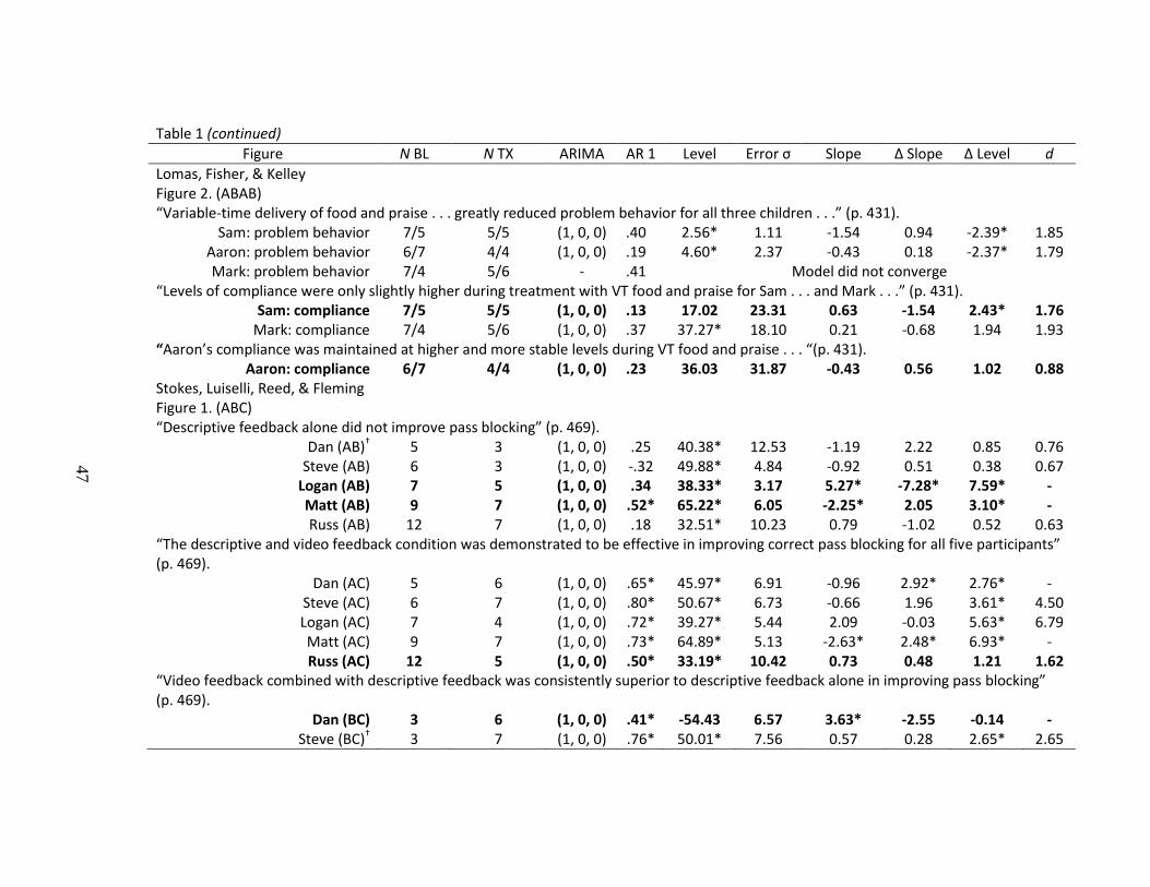
47

Table 1 (continued)


Lomas, Fisher, & Kelley Figure 2. (ABAB) “Variable-time delivery of food and praise . . . greatly reduced problem behavior for all three children . . .” (p. 431).

Sam: problem behavior 7/5 5/5 (1, 0, 0) .40 2.56* 1.11 -1.54 0.94 -2.39* 1.85 Aaron: problem behavior 6/7 4/4 (1, 0, 0) .19 4.60* 2.37 -0.43 0.18 -2.37* 1.79 Mark: problem behavior 7/4 5/6 - .41 Model did not converge

“Levels of compliance were only slightly higher during treatment with VT food and praise for Sam . . . and Mark . . .” (p. 431). Sam: compliance 7/5 5/5 (1, 0, 0) .13 17.02 23.31 0.63 -1.54 2.43* 1.76

Mark: compliance 7/4 5/6 (1, 0, 0) .37 37.27* 18.10 0.21 -0.68 1.94 1.93 “Aaron’s compliance was maintained at higher and more stable levels during VT food and praise . . . “(p. 431).

Aaron: compliance 6/7 4/4 (1, 0, 0) .23 36.03 31.87 -0.43 0.56 1.02 0.88 Stokes, Luiselli, Reed, & Fleming Figure 1. (ABC) “Descriptive feedback alone did not improve pass blocking” (p. 469).

Dan (AB)† 5 3 (1, 0, 0) .25 40.38* 12.53 -1.19 2.22 0.85 0.76 Steve (AB) 6 3 (1, 0, 0) -.32 49.88* 4.84 -0.92 0.51 0.38 0.67

Logan (AB) 7 5 (1, 0, 0) .34 38.33* 3.17 5.27* -7.28* 7.59* - Matt (AB) 9 7 (1, 0, 0) .52* 65.22* 6.05 -2.25* 2.05 3.10* - Russ (AB) 12 7 (1, 0, 0) .18 32.51* 10.23 0.79 -1.02 0.52 0.63

“The descriptive and video feedback condition was demonstrated to be effective in improving correct pass blocking for all five participants” (p. 469).

Dan (AC) 5 6 (1, 0, 0) .65* 45.97* 6.91 -0.96 2.92* 2.76* - Steve (AC) 6 7 (1, 0, 0) .80* 50.67* 6.73 -0.66 1.96 3.61* 4.50 Logan (AC) 7 4 (1, 0, 0) .72* 39.27* 5.44 2.09 -0.03 5.63* 6.79 Matt (AC) 9 7 (1, 0, 0) .73* 64.89* 5.13 -2.63* 2.48* 6.93* - Russ (AC) 12 5 (1, 0, 0) .50* 33.19* 10.42 0.73 0.48 1.21 1.62

“Video feedback combined with descriptive feedback was consistently superior to descriptive feedback alone in improving pass blocking” (p. 469).

Dan (BC) 3 6 (1, 0, 0) .41* -54.43 6.57 3.63* -2.55 -0.14 - Steve (BC)† 3 7 (1, 0, 0) .76* 50.01* 7.56 0.57 0.28 2.65* 2.65

48

Table 1 (continued)


Logan (BC) 5 4 (1, 0, 0) .58* 72.94* 5.27 -3.61* 2.36 6.30* - Matt (BC) 7 7 (1, 0, 0) .36 67.99* 6.53 0.88 0.04 0.91 0.92 Russ (BC) 7 5 (1, 0, 0) .59* 46.73 5.99 -1.04 1.58 2.24 3.67

Stokes, Luiselli, & Reed Figure 1. (AB) “His correct tackling also increased with intervention . . . (p. 511).

Mikea 12 10 (1, 0, 0) .74* 29.01* 7.22 0.08 4.21* 0.68 - Falcomata, Roane, Feeney, & Stephenson

Figure 1. Top panel (ABAB) “Rates of elopement were elevated during the free-access condition . . . relative to rates during the blocking condition” (p. 515).

Elopement 3/8 5/12 (1, 0, 0) .31* 1.50* 0.43 -0.65 1.00 -3.66* 2.63 Raiff & Dallery Figure 1. (ABA) “When the intervention was introduced, an increase in the frequency of testing occurred” (p. 489).

Talia (AB) 5 5 (1, 0, 0) .55 0.80 1.22 1.47 -1.33 3.41* 3.98 Bonita (AB) 5 5 (1, 0, 0) .30 1.45 1.33 0.65 -0.69 2.61* 2.68

Edward (AB) 5 5 (1, 0, 0) .27 2.78 0.28 2.23 -1.26 1.12 1.21 Andrea (AB) 5 5 (1, 0, 0) .51 1.02 1.30 0.10 1.80 1.78 2.00

“Removing the intervention resulted in a decrease in the frequency of testing . . .” (p. 489). Talia (BA) 5 5 (1, 0, 0) .51 6.88 1.38 -0.20 -0.94 -0.73 1.02

Bonita (BA) 5 5 (1, 0, 0) -.05 5.84 1.21 -0.01 -0.39 -1.58 1.67 Edward (BA) 5 5 (1, 0, 0) .35 3.98* 0.22 0.04 4.15* -5.44* - Andrea (BA) 5 5 (1, 0, 0) .51 0.35 0.96 2.80* -2.46 -3.99* -

Leon, Hausman, Kahng, & Becraft

Figure 1. (ABCD) “The implementation of differential reinforcement during nonbusy activities resulted in an increase in appropriate responding during nonbusy activities in Pair 1 . . .” (p. 527).

Pair 1: Communicationc 4 50/10/21 (3, 0, 0) .41* 73.84* 20.55 -0.25 0.31 -0.34 0.31

49

Table 1 (continued)


Carter Figure 1. Middle panel (ABABC) “. . . presentation of a high-preference edible item contingent on compliance increased compliance and reduced destructive behavior . . .” (p. 545).

Compliance (ABAB) 5/4 8/3 (1, 0, 0) .54* 33.44* 7.92 -0.61 1.57 5.16* 3.51 Destructive behavior (ABAB) 5/4 8/3 (1, 0, 0) .47* 52.38* 9.25 0.38 -3.61* -1.81 -

“. . . the provision of a 30-s break from the tasks for both compliance and destructive behavior produced levels of responding similar to those observed during baseline.. (p. 545).

Compliance (AAC) 5/4 6 (1, 0, 0) .14 33.58* 8.37 -0.61 -2.46* 3.90* - Destructive behavior (AAC) 5/4 6 (1, 0, 0) .46 53.12* 8.01 0.15 -0.06 -1.94 2.24

Grauvogel-Macaleese & Wallace Figure 2. “When peers implemented differential reinforcement, off-task behavior immediately decreased for all three participants . . .” (p. 549).

Scott (ABAB) 3/3 7/4 (1, 0, 0) .45* 63.44* 14.10 2.40* -1.75 -4.54* - Zane (AB) 5 9 (1, 0, 0) .55* 46.43* 12.55 3.10* -3.55* -6.83* - Drew (AB) 7 12 (1, 0, 0) .76* 51.01* 11.15 1.18 -0.99 -5.53* 5.28

Athens & Vollmer Figure 3. “. . . for both participants, the relative rates of problem behavior and appropriate behavior were sensitive to the reinforcement duration . . .” (p. 578). Justin (ABCACA)

Problem behavior (ACACA)b 4/10/14 14/20 (5, 0, 0) .58* 2.40* 0.80 -3.04* 0.17 -0.96 - Compliance (ACACA) 4/10/14 14/20 (5, 0, 0) .30* 0.24 0.64 1.93 0.56 -0.30 0.17

Lana (ABAB) Problem behavior (ABAB)a 6/9 13/11 (5, 0, 0) .68* 1.67* 0.68 0.12 -0.58 -0.77 0.74

Mand (ABAB)b 6/9 13/11 (5, 0, 0) .76* 0.11 0.45 1.90 -0.43 0.47 0.51

50

Table 1 (continued)


Figure 4. Justin (ABCAC) “In the 1 HQ/1 LQ condition, rates of problem behavior decreased, and appropriate behavior increased” (p. 579).

Problem behavior (AB) 5 14 (1, 0, 0) -.05 5.31* 1.46 -2.02 2.18* -0.46 - Compliance (AB) 5 14 (1, 0, 0) .13 3.39* 1.21 -2.22* 1.52 4.24* -

“Problem behavior decreased, and appropriate behavior increased to high levels during the return to the 3 HQ/1 LQ condition” (p. 580). Problem behavior (AC) 9 7 (1, 0, 0) -.29 2.16* 0.70 -3.46* -0.51 2.21* -

Compliance (AC) 9 7 (1, 0, 0) .06 5.23* 1.34 -0.78 1.61 -1.52 1.35 “In summary, results of the quality analyses indicated that . . . the relative rates of both problem behavior and appropriate behavior were sensitive to the quality of reinforcement available for each alternative” (p. 581).

Problem behavior (ABCAC) 5/9 14/10/7 (1, 0, 0) -.07 2.92* 1.20 -2.88* 1.41 -2.91* - Compliance (ABCAC)b 5/9 14/10/7 (5, 0, 0) .44* 1.00 1.44 3.49* -1.98 0.70 -

Kenneth (ABABACBC) “In the 1 HQ/1 LQ condition, rates of problem behavior decreased, and appropriate behavior increased” (p. 580).

Problem behavior (AB) 6 15 (1, 0, 0) .57* 4.54* 1.75 0.21 -0.71 -0.21 0.23 Mand (AB) 6 15 (1, 0, 0) .54* -0.05 0.51 0.28 1.45 -2.14* 1.67

“. . . we conducted the 3 HQ/1 LQ condition, and problem behavior decreased to rates lower than observed in previous conditions and appropriate behavior increased to high rates” (p. 580).

Problem behavior (ABABAC)a 6/15/5/4/10

19 (5, 0, 0) .67* 4.34* 1.41 -2.21* 0.32 -0.97 -

Mand (ABABAC)c 6/15/5/4/10

19 (5, 0, 0) .64* -0.17 0.62 5.97* -1.14 -0.53 -

“In summary, results of the quality analyses indicated that . . . the relative rates of both problem behavior and appropriate behavior were sensitive to the quality of reinforcement available for each alternative” (p. 581).

Problem behavior (ABABACBC)c 6/5/10 15/4/19/8/ 22

(5, 0, 0) .58* 4.99* 1.54 -1.35 0.94 -2.19* 1.36

Mand (ABABACBC)d 6/5/10 15/4/19/8/ 22

(5, 0, 0) .57* 0.17 0.72 1.59 -1.05 1.84 1.14

51

Table 1 (continued)


Figure 5. Corey (ABCAC) “In summary, results of the delay analysis indicate that the relative rates of problem behavior and appropriate behavior were sensitive to the delay to reinforcement following each alternative” (p. 582).

Problem behavior 23/6 21/17/44 (5, 0, 0) .27* 3.28* 2.23 -0.14 -0.77 -0.46 0.16 Manda 23/6 21/17/44 (5, 0, 0) .17 1.60* 1.12 -0.14 -0.09 0.00 0.00

Henry (ABACABAC) “In a reversal to 0-s/0-s delay baseline, there was a slight increase in problem behavior from the previous condition and a decrease in appropriate behavior” (p. 582).

Problem behavior (BA) 6 8 (1, 0, 0) .22 0.46 0.79 1.55 0.83 -1.60 1.75 Mand (BA) 6 8 (1, 0, 0) .00 1.87* 0.75 -2.45* -0.79 2.28* -

“During the 0-s/60-s delay condition, there was a decrease in problem behavior to zero rates and an increase in appropriate . . . (p. 582). Problem behavior (AB) 6 11 (1, 0, 0) .59* 0.48 0.75 2.21* -3.77* 0.00 -

Mand (AB) 6 11 (1, 0, 0) .47 1.67* 0.64 -2.25* 2.79* 2.25* - “In summary, results of the delay analysis indicate that the relative rates of problem behavior and appropriate behavior were sensitive to the delay to reinforcement following each alternative” (p. 582).

Problem behavior 4/6/ 12/4

8/11/11/16 (5, 0, 0) .55* 1.50* 0.80 -0.20 -0.35 0.18 0.13

Mand

4/6/ 12/4

8/11/11/16 (5, 0, 0) .38* 0.74 0.82 -0.60 1.14 0.63 0.35

Figure 6. George (ABAB) “In summary, results of the combined analyses indicate that for these participants the relative rates of problem behavior and appropriate behavior were sensitive to a combination of the quality, delay, and duration of reinforcement following each alternative” (p. 584).

Problem behavior 7/6 7/10 (5, 0, 0) .45* 3.60* 1.39 -1.89 1.37 -2.63* 1.94 Manda 7/6 7/10 (1, 0, 0) -.06 0.03 0.47 1.17 0.19 3.92* 1.55

52

Table 1 (continued)


Clark (ABAB) “In summary, results of the combined analyses indicate that for these participants the relative rates of problem behavior and appropriate behavior were sensitive to a combination of the quality, delay, and duration of reinforcement following each alternative” (p. 584).

Problem behaviora 6/5 8/10 (1, 0, 0) .77* 2.91* 0.61 -1.63 1.44 -4.09* 4.07 Manda 6/5 8/10 (1, 0, 0) .51* 1.13* 0.53 -2.43* 3.79* 0.59 -

Wilder, Allison, Nicholson, Abellon, & Saulnier

Figure 1. Ricky (ABACABAC) “For Ricky, compliance improved when the guided compliance procedure was conducted” (p. 606).

Compliance (AACAAC) 3/3/3/3 6/8 (1, 0, 0) .58* 6.91 23.11 -0.77 1.87 3.23* 1.99 Ian (ABACABADAD) “For Ian, contingent access to preferred edible items initially appeared to be effective in increasing compliance, but compliance decreased toward the end of this phase” (p. 606).

Compliance (AC) 5 6 (1, 0, 0) .37 1.85 24.35 -0.14 -1.21 3.71* 3.78 “Therefore, a response-cost component was added, which increased compliance to high levels” (p. 607).

Compliance (ADAD) 7/3 3/5 (1, 0, 0) .50* 3.47 18.75 0.38 -0.76 5.70* 5.08 Andy (ABACADABACAD) “. . . contingent access to preferred edible items was immediately effective in increasing compliance” (p. 607).

Compliance (AD) 3 6 (1, 0, 0) .66* 4.03 16.49 -0.24 0.43 4.05* 5.03 Figure 2. Ricky (ABACABAC) “For Ricky, problem behavior occurred exclusively during the guided compliance conditions, but appeared to subside during each implementation” (p. 607).

Problem behavior (AACAAC) 3/3/3/3 6/8 (1, 0, 0) .07 -1.58 12.45 0.36 -2.16* 3.94* - Ian (ABACABADAD) “Ian exhibited most of his problem behavior during rationale conditions” (p. 608).

Problem behavior (ABAB) 5/9 8/5 (1, 0, 0) .46* 32.75 26.72 -0.28 0.22 -0.07 0.07

53

Table 1 (continued)


Figure 3. Ed (ABACABAC) “For Ed, compliance improved when he received access to his preferred edible item contingent on compliance” (p. 609).

Compliance (ACAC) 3/4 6/7 (1, 0, 0) .62* 5.15 22.66 0.49 1.16 1.93 1.71 Carl (ABACABAC) “For Carl, contingent access to preferred edible items was also effective in increasing compliance” (p. 609).

Compliance (ACAC) 3/3 3/16 (1, 0, 0) .57* 1.06 4.31 -0.42 0.53 37.44* 22.74 Sam (ABACABAC) “For Sam, contingent access to preferred edible items was also effective in increasing compliance” (p.609).

Compliance (ACAC) 3/3 3/25 (1, 0, 0) .42* 18.73 17.54 -0.84 0.60 8.29* 4.85 Carbone, Sweeney-Kerwin, Attanasio, & Kasper

Figure 1. (AB) “Tony’s mean responding showed a threefold increase in unprompted vocal responding . . .” (p. 707).

Tonyb 10 21 (5, 0, 0) .66* 9.58* 6.27 0.16 0.76 3.09* 2.30 “Both Ralph’s and Nick’s manual sign mands were accompanied by very few vocal responses during baseline, but demonstrated substantial increases in unprompted vocalizations during treatment” (p. 707).

Ralph 17 10 (1, 0, 0) .67* 1.18 5.51 -0.12 0.87 1.51 1.57 Nick 21 7 (1, 0, 0) .59* 1.13 1.46 0.11 -0.31 -0.33 0.40

Ulke-Kurkcuoglu & Kircaali-Iftar Figure 1. (ABABA)

“All participants except Yavuz consistently displayed higher levels of on-task behaviors during choice conditions than during baseline” (p. 719).

Utku 4/4/4 4/4 (1, 0, 0) .47* 62.45* 5.52 4.13* -2.01 5.91* - Alp 4/4/4 4/4 (1, 0, 0) .53* 65.04* 3.52 6.07* -0.79 6.34* -

Selim 4/4/4 4/4 (1, 0, 0) .57* 70.97* 3.62 3.10* -0.02 4.64* - Yavuz 4/4/4 4/4 (1, 0, 0) .65* 66.03* 2.51 16.08* -6.11* 13.31* -

54

Table 1 (continued)


“Yavuz’s on-task behavior during the last baseline condition was similar to his on-task behavior in the choice conditions” (p. 719). Yavuz (BBA) 4 4/4 (1, 0, 0) .23 95.83* 1.60 1.62 0.43 -3.13* 3.85

Roscoe, Kindle, & Pence Figure 1. Bottom panel (ABAB) “During the first FCT intervention phase [as well as return to the FCT intervention], she did not exhibit aggression and emitted the communication response at mostly short latencies and at a high frequency. . .” (p. 726).

Aggression 3/3 5/9 (1, 0, 0) .46* 42.94 65.99 -0.73 0.51 5.45* 3.80 Communication 3/3 5/9 (1, 0, 0) .30 304.88* 95.74 -1.11 0.53 -3.17* 2.20

Travis & Sturmey Figure 1. Bottom panel (ABAB) “The immediate success of this intervention . . . “(p. 748).

Nondelusional statements 4/4 5/4 (1, 0, 0) .55* 0.61* 0.15 -2.29* 5.02* 6.61* - Delusional statements 4/4 5/4 (1, 0, 0) .58* 1.45* 0.16 -0.07 -1.66 -7.95* 6.38

Wilder, Nicholson, & Allison Figure 1. Top panel (ABABACAC) “Ralph’s compliance was generally low during baseline . . . . However, when physical guidance was added, his compliance increased and remained at high levels” (p. 753).

Compliance (ACAC) 3/6 10/5 (1, 0, 0) .64* 11.83 31.61 0.29 1.35 -0.21 0.21 Middle panel (ABABACADACAD) “During the first advance notice plus physical guidance phase, compliance remained relatively low . . .” (p. 753).

Compliance (AC) 4 7 (1, 0, 0) .37 -1.21 14.99 0.13 -0.21 0.50 0.62 “During the physical guidance only phase, compliance increased and remained at high levels . . .” (p. 753).

Compliance (AD) 3 11 (1, 0, 0) .62* 4.21 25.27 -0.24 0.73 -0.07 0.08 Compliance increased again during the second advance notice plus physical guidance phase. . .” (p.753).

Compliance (AC) 3 8 (1, 0, 0) .41* 48.89 29.74 -1.03 1.05 2.26 2.49 Compliance . . . increased to high, stable levels during the second physical guidance phase . . .” (p. 753).

Compliance (AD) 9 9 (1, 0, 0) .04 60.76* 25.15 -2.20* -0.23 5.27* -

55

Table 1 (continued)


Bottom panel (ABABACACAD) “When physical guidance was added, compliance increased . . .” (p. 753).

Compliance (ACAC) 3/4 8/10 (1, 0, 0) .52* 12.84 24.74 -0.31 0.69 0.90 0.82 “During the last phase, advance notice was removed and physical guidance alone was implemented. Compliance improved . . . and remained at high levels . . . during this phase” (p. 753).

Compliance (AD) 4 7 (1, 0, 0) .70* -3.05 14.24 0.31 3.56* -2.29* - Miller, Lerman, & Fritz Figure 1. “. . . the percentage of trials with reprimands decreased during the first extinction phase . . . Cindy’s responding was similar to that during her first extinction phase, although suppression was less pronounced” (p. 771).

Cindy (ABAB) 3/4 4/8 (1, 0, 0) .38 71.41* 30.05 1.19 -1.23 -0.55 0.49

Note. The following information is included in the first column: authors of the publication, figure label as it is presented in

the publication, experimental design presented using capital letters in the parenthesis. Unless otherwise indicated with the

superscript (†), each ITSA model was determined based on four parameters: level, slope, change in slope and change in

level. N BL = number of observations in the baseline or reference phase; N TX = number of observations in the treatment

phase; ARIMA = autoregressive moving average model; AR 1 = autoregressive term 1; Level = intercept; Error σ =

standard error estimate; Slope = t-test statistic for linear trend of the time series; Δ Slope = t-test statistic for change in

slope at the interruption point; Δ Level = t-test statistic for change in level at the interruption point; d = Cohen’s d effect

size; Cohen’s d effect size is not available for time series with significant slope or change in slope. a significant AR 2

b significant AR 2 and AR 3

c significant AR 2, AR 3, and AR 4

d significant AR 2, AR 3, AR 4 and AR 5

† ITSA model estimated separately for slope and change in slope due to small number of observation that affected model’s

stability

*p < .05

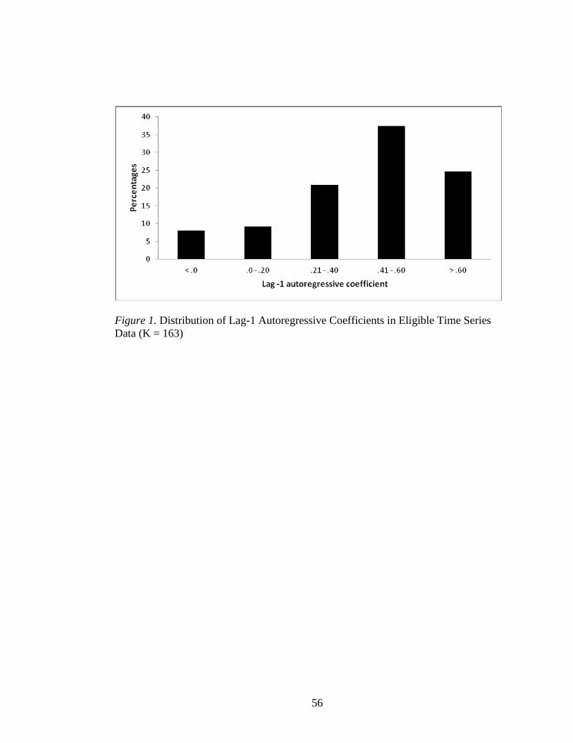
56


Data (K = 163)

57


Data (k = 98)

58

Statistical Analysis

Significant Not Total

Graphical

Analysis

Significant

79

52

131

Not

8

15

23

Total 87 67 154 Figure 3. Agreement between graphical analysis and statistical analysis

59


application.

Note. Figure reproduced from the data extracted using UnGraph® software from

Lomas, Fisher, & Kelly, 2010 (p. 430).

60


application.


Lomas, Fisher, & Kelly, 2010 (p. 430).

61

Figure 6. Graphical presentation of the data illustrated in the second example of ITSA

application.

Note. Figure reproduced from the data extracted using UnGraph® software from Van

Houten et al., (2010) (p. 377).

62


application.


Athens, & Vollmer (2010) (p. 580).

63


application.


Athens, & Vollmer (2010) (p. 580).

64

CHAPTER 3


Kazdin Textbook Examples

Manuscript will be submitted to Psychological Methods

65

Abstract



analysis area among the advocates of visual analysis and proponents of interrupted

time-series analysis (ITSA). To address this debate, a head-to-head comparison of

both methods was performed, as well as an overview of serial dependency, effect sizes

and sample sizes.

Method. Conclusions drawn from visual analysis of graphs obtained from the

textbook by Alan E. Kazdin (2011) were compared with findings based on ITSA of

the same data. This comparison was made possible by the software, called UnGraph®

which permits recovery of raw data from graphs and the application of ITSA.

Results. ITSA was successfully applied to 97% of examined time-series data with

numbers of observations ranging from 10 to 68. Over 65% of the data had moderate to

high level first order autocorrelations (> .40). Large effects sizes (≥ .80) were found

for 75% of eligible studies. Comparison of the conclusions drawn from visual analysis

and ITSA revealed an overall moderate level of agreement (Kappa = .44).


applied behavior analysis research and can facilitate evaluation of intervention effects,

particularly when specific characteristics of single-subject data limit the reliability and

validity of visual analysis. These two methods should be viewed as complimentary

and used concurrently.

66

Keywords: Applied Behavior Analysis, Single-subject Studies, Visual Analysis,

Interrupted Time-series Analysis, Effect Size, Serial Dependency

67


Kazdin Textbook Examples

Group-level and single-subject research designs are two methodological models

employed for analyzing longitudinal research. The first model is based on data

obtained from a large number of individuals and provides average estimates of

longitudinal trajectories of behavior change based on group-level data, emphasizing

between-subject variability. A significant limitation of group-level designs, also

known as nomothetic designs, is the inability to capture high levels of variability and

heterogeneity within the studied populations (Molenaar, 2004). Further, group-level

designs emphasize central tendencies of the population and consequently obscure

natural patterns of behavior change, their multidimensionality and unique variability

within each individual (Molenaar & Campbell, 2009).

The second methodological approach employed in longitudinal research is based

on data obtained from one individual or unit (n = 1) through intensive data collection

over time. Single-subject designs, also known as idiographic designs, examine

individual-level data, that allows for highly accurate estimates of within-subject

variability and longitudinal trajectories of each individual’s behavior. Idiographic

methodology characterizes highly heterogeneous processes, which consequently allow

for more accurate inferences about the nature of behavior change specific to an

individual (Velicer & Molenaar, 2013). Single-subject designs address the limitations

of group-level designs and present several advantages. They allow for a highly

accurate assessment of the impact of the intervention for each individual while group-

68

level designs provide information about the effectiveness of the intervention for an

“average” person, rather than any person in particular (Velicer & Molenaar, 2013).

In addition, single-subject research allows studying longitudinal processes of

change with much better precision than group-level designs, due to a higher number of

data points and better controlled variability of the data. Also, it can be applied to

populations that are otherwise difficult to recruit in numbers large enough to allow for

a group-level design (Barlow, Nock, & Hersen, 2009; Kazdin, 2011).

Methods of evaluating single-subject studies


based on single-subject designs. Visual analysis of the graphs presenting experimental

data is a commonly used approach in applied behavior analysis research, while

interrupted time-series analysis (ITSA) is a statistical method used in research fields,

such as electrical engineering, economics, business, and other areas of psychology, to

name just a few. The use of visual analysis preceded the development of quantitative

methods like time series analysis which required high speed computers to implement.

Visual analysis

The most basic experimental model used in single-subject research is an A-B

design with a well defined target behavior that is examined before and after the

intervention. The first phase (A) of the design consists of multiple baseline

observations that assess the pre-intervention characteristics of the behavior. In the

second phase (B) of the design, the treatment component of the experiment is

introduced and changes in behavior are examined (Barlow et al., 2009; Kazdin, 2011).

69

The visual analysis of the graph, performed by a judge or a rater, is based on a set

of criteria that evaluate and compare the characteristics of phase A and B and examine

whether behavior changes in phase B are a result of the intervention. The baseline (A)

phase provides information about the descriptive and predictive aspects of the target

behavior, such as stability and variability. Stable behavior, characterized by the

absence of a trend or slope in the data, indicates that the targeted behavior neither

increases nor decreases on average over time during the baseline phase (Kazdin,

2011). Variability of the data is characterized by the changes in the behavior within

the range of possible low and high levels (Barlow et al., 2009). Single-subject

experiments are evaluated based on magnitude and rate of change between phase A

and B. The magnitude of change is based on variability in level and slope of the data.

Changes in level refer to average changes in the frequency of target behavior, whereas

changes in slope refer to shifts in direction of the behavior across different phases. The

mean is the average for all data in a particular phase. If the series is stable, the level

will equal the slope. Changes in level and slope are independent from each other. Rate

of change is based on changes in trend or slope of the data and latency of change.

Trend analysis provides information on systematic increases or decreases in the

behavior across phases, whereas latency of change refers to the amount of time

between the termination of one phase and changes in behavior (Kazdin, 2011).

Visual analysis, although guided by the set of criteria described above, is not

based on any specific decision making rules and it is mostly driven by subjective

evaluation of the intervention effects. Advocates of this approach argue that large

intervention effects are evident and provide unequivocal conclusions that can be easily

70

observed by independent judges. Further, it is argued that the subjective evaluation of

intervention effects has a minimal impact on reliability and validity of the conclusions

drawn from the graphs presenting large and therefore easily observable treatment

effects, since only those are considered to have significant clinical implications (Baer,

1977; Kazdin, 2011). This concept is particularly promoted in the field of applied

behavior analysis.

Proponents of visual analysis acknowledge that certain characteristics of single-

subject data can significantly impair the ability to accurately evaluate intervention

effects. The presence of slope in the baseline phase of the experiment may negatively

affect the evaluation of the experiment, especially when the trend of the targeted

behavior is moving in the same direction as would be expected due to treatment

effects. High variability of the data may also interfere with the validity of the

conclusions. For example, accuracy of the evaluation of intervention effects on

disruptive behavior can be significantly affected by a pattern of behavior that is

decreasing (getting better) over time. Also high variability of the behavior, such as

extreme fluctuations from none to high frequency of disruptive behavior can limit the

ability to draw valid conclusions about intervention effects (Kazdin, 2011). However,

it is argued that the rationale for using visual analysis is to highlight large (i.e. easily

observable) intervention effects and disregard small (i.e. not easily observable) effects.

It is concluded that visually undetected intervention effects have insignificant clinical

impact. Proponents of visual analysis state that the conservative approach to

evaluating intervention effects guarantees highly accurate and consistent conclusions

across independent judges, as well as reduces unknown probability of Type I error rate

71

and consequently increases the probability of Type II error rate (Baer, 1977; Kazdin,

2011).

In the recent literature, some of the visual analysis advocates have discussed the

problem of the lack of effect size estimation which results in an inability to perform

meta-analytic reviews single-subject experiments. As stated by Kazdin (2011), the

single-subject research field would benefit from the ability to integrate a large number

of studies in a systematic way that would allow drawing broader conclusions

regarding intervention effects that would generalize beyond single experiments.

However, to date there is no consensus regarding guidelines for interpreting effect

sizes calculated based on supplementing visual analysis methods commonly used

among single-case researchers. Brossart, Parker, Olson, and Mahadevan (2006)

compared five analytic techniques frequently used in single-subject research applied to

the same data and concluded that each analytical approach was strongly influenced by

serial dependency, and the obtained results based on each method varied so much that

it prohibited the development of any reliable effect-size interpretation guidelines.

Inability to estimate effect sizes based on currently used analytical methods leaves

meta-analytic approaches out of reach in the field of single-subject research. A

noteworthy study by Hedges, Pustejovsky and Shadish (2012) proposed new effect

size that is comparable to Cohen’s d, frequently used in group-level designs. It is

applied across single-subject cases and it can be used in studies with at least three

independent cases. This new approach can be applied in meta-analytic research and

warrants further examination.

72


analysis led to inconsistent conclusions about the intervention effects across different

raters. The inter-rater agreement among judges who reviewed the same graphs was

relatively poor, ranging on average from .39 to .61 (Jones, Weinrott, & Vaught, 1978;

DeProspero & Cohen, 1979; Ottenbacher, 1990), suggesting that visual analysis is not

a reliable method for assessing intervention effects of single-subject data. Higher

complexity of the data and experimental design resulted in less consistent conclusions.

Factors like high variability of the data, inconsistent patterns of behavior over time,

changes in slope, and small changes in level of the data were associated with lower

agreement rates across judges (DeProsper & Cohen, 1979; Ottenbacher, 1990).

In addition, Matyas and Greenwood (1990) showed that a positive autocorrelation

and high variability in the data tend to increase Type I error rates. These findings

suggest that the claimed advantages of visual analysis resulting in a reduced in Type I

error rates are highly overstated.

Several studies demonstrated that higher levels of serial dependency in a single-

subject data lead to higher rates of disagreement between visual and statistical analysis

(Bengali & Ottenbacher, 1998; Jones et al., 1978; Matyas & Greenwood, 1990). One

study by Jones et al. (1978) showed that the highest level of agreement between the

two methods was found when there were non-statistically significant changes in the

behavior and the lowest agreement occurred when there were significant effects of the

intervention. These findings suggest that statistically significant results may be more

often overlooked by visual analysis than non-significant results and that the highest

73

agreement between these two methods occurs when there is no serial dependency in

the data and intervention effects are insignificant.

Interrupted time-series analysis

Interrupted time-series analysis (ITSA) is a statistical method used to examine

intervention effects of single-subject study designs. It is based on chronologically

ordered observations obtained from a single subject or unit. An inherent property of

time-series data is serial dependency that reflects the impact of previous observations

on the current observation and violates the assumption of independence of errors,

which can significantly affect the validity of the statistical test. Serial dependency,

examined by the magnitude and direction of autocorrelations between observations

spaced at different time intervals (lags), directly impacts error term estimation and

validity of the statistical test. Negative autocorrelations produce an overestimation of

the error variance, which leads to conservative bias and increases Type II error rate,

whereas positive autocorrelations lead to underestimation of the error variance, and

cause liberal bias and increase Type I error rates (see Velicer & Molenaar, 2013 for an

illustration).

The most widely used model for examining serial dependency in the data is the

autoregressive integrated moving average (ARIMA) model. It consists of three

elements to be evaluated. The autoregressive term (p) estimates the extent to which the

current observation is predictable from preceding observations and the number of past

observations that impact the current observation. The moving average term (q)

estimates the effects of preceding random shocks on current observation. The

integrated term (d) refers to the stationarity of the series. Stationarity of time-series

74

data requires the structure and the parameters of the data, such as mean, variance and

the patterns of the autocorrelations to remain the same across time for the series. Non-

stationary data requires differencing in order to keep the series at a constant mean

level, otherwise reliability of the assessed intervention effects can be compromised

(Glass, Willson, & Gottman, 2008).

The ITSA method is able to measure the degree of the serial dependency in the

data and statistically remove it from the series, allowing for an unbiased estimate of

the changes in level and trend across different phases of the experiment (Glass et al.,

2008). In addition, after accounting for serial dependency in the data, ITSA facilitates

an estimate of Cohen’s d effect size (Cohen, 1988), which is the most commonly used

measure of intervention effects in behavioral sciences research with widely

implemented interpretative guidelines.

ITSA limitations

Although, the most recommended method for removing serial dependency from

single-subject data is implementing an ARIMA model (Glass et al., 2008), some

researchers call attention to some drawbacks of ITSA related to accurate ARIMA

model estimation and limited utility in applied behavior analysis studies (Ottenbacher,

1992; Kazdin, 2011). Identifying the correct ARIMA model has been shown to be

often unreliable, leading to model misidentification (Velicer & Harrop, 1983).

However this issue has been addressed through the general transformation method,

which uses the ARIMA model for lag-5 autocorrelation (5, 0, 0) that was shown to be

simpler and more accurate than other model specification methods (Velicer &

McDonald, 1984). For shorter time-series data a simpler model based on lag-1

75

autocorrelation (1, 0, 0) is sufficient when applied to data that does not require

forecasting (Simonton, 1977). Simulation studies have shown that these procedures

are very accurate (Harrop & Velicer, 1985; Harrop & Velicer, 1990).

Another disadvantage of the ARIMA procedure has been associated with the

requirement of a large number of observations. A minimum of 35-40 observations or

even as high as 25 observations per phase were recommended (Glass et al., 2008;

Ottenbacher, 1992) in order to correctly identify an ARIMA model. However,

application of predetermined ARIMA model allows for reliable evaluation of shorter

data series. In addition, proponents of visual analysis argue that ITSA may not be a

suitable analytical approach for experimental designs that reach beyond the basic AB

model, such as alternating treatment designs or multiple baseline designs (Barlow et

al., 2009; Kazdin, 2011).

Study Aims

This study will perform a head-to-head comparison of the conclusions drawn

from visual analysis of graphically presented data with the findings based on

interrupted time-series analysis of the same data. The study will use graphical data

based on published single-subject studies included in the textbook by Kazdin (2011).

The text was selected because it is a leading text on the topic used by applied

researchers and the author strongly promotes the use of visual analysis rather than

quantitative analysis methods. In a related study, all the studies published in a leading

journal (Journal of Applied Behavior Analysis, 2010) were evaluated in the same way

(Harrington & Velicer, 2013).

76

The aim of this study is to examine the level of agreement between these two

methods, as well as degree of serial dependency in single-subject data, and estimate

the effect size for each study. This comparison is made possible by the development of

a statistical program called UnGraph® software version 5.0 (Biosoft, 2004), which

permits the recovery of raw data and the application of interrupted time series

analysis.

Method

Sample

Graphical data was obtained from the book titled “Single-Case research designs:

Methods for clinical and applied settings” by Alan E. Kazdin (2011), who is currently

the leading advocate of visual analysis of single-subject studies. The book is a widely

used textbook within the applied psychology area and provides numerous examples of

graphs presenting single-subject experimental data with corresponding evaluations of

intervention effects based on visual analysis.

For a graph to be included in this study, it was required to meet the following

inclusion criteria: (1) present actual data (not simulated); (2) present already published

data; (3) present interrupted time-series data; (4) present a minimum of three

observations in each phase of the design in order to estimate a full four parameter

model; (5) present baseline and treatment phases of an experimental design; (6)

include corresponding description of the conclusions drawn from the visual analysis of

77

the graph; and (7) present well defined data points (observations) in the graph. Graphs

presenting cumulative data or alternating-treatment designs were not eligible.

Procedure

Eligible graphs were scanned and electronically imported into UnGraph®

software version 5.0 (Biosoft, 2004). Next, data presented in each graph was extracted

using the UnGraph® software function of coordinate system that defined each graph’s

structure and scale. Then, sequentially ordered data recorded in a time-series data

format was exported into a Microsoft Excel® spreadsheet.

Validity and reliability of UnGraph®

software

UnGraph® software has been previously examined for its validity and reliability

when extracting data from graphs representing single-case designs (Shadish et al.,

2009). Results of this study indicated high validity and reliability of the extracted data

from graphs, with .96 as an average correlation coefficient between two raters.

Analysis

Interrupted time-series analyses (ITSA) were used to evaluate intervention effects

of each single-subject study based on the data collected using UnGraph® software.

Identification of the ARIMA model was performed in a series of steps. First, level of

autocorrelation in the data was evaluated based on autocorrelation function (ACF) and

partial autocorrelation function (PACF). These two functions refer to autoregressive

and moving average parameters and estimate whether negative or positive correlation

was present in the data series, as well as in how many lags the correlation was present.

78

Also, the stationarity parameter (d) was evaluated, and if required, differencing of the

data was performed.

Second, values of each parameter were estimated and the fit of the ARIMA model

was evaluated. The best fitting model resulted in uncorrelated residuals. In cases when

the residuals were correlated, the model identification process was repeated and a new

model was evaluated (Barlow et al., 2009; Glass et al., 2008). Once a correctly

identified ARIMA model was applied to single-subject data, parameters such as trend,

change in trend, level, change in level, as well as mean and variability of the series

were evaluated. Intervention effects were examined based on changes in slope and

level across the experimental phases of the design. In addition, for studies where no

significant slope or change in slope was present, Cohen’s d effect size was calculated

to examine the magnitude of the behavior change due to the intervention. Analyses

were performed in SAS version 9.2. This study was approved by the University of

Rhode Island Institutional Review Board.

Description of the visual analysis of graphs presented in the textbook written by

Kazdin (2011) was used to perform a head-to-head comparison of the findings based

on each method. These comparisons were based on conclusions made in regards to

trend, change in trend, variability of the data and change in level of the data across

different experimental phases of the experiment.

Results

Sample

A total of 134 graphs presenting time-series data based on published studies were

reported in the textbook. After reviewing the content of the graphs, 60 met eligibility

79

criteria and were included in this study. Excluded publications presented less than 3

observations in at least one phase of the design (k = 26), presented cumulative data or

alternating-treatment designs (k = 17), did not present interrupted time-series data (k =

14), or did not meet one of the other eligibility criteria (e.g. included aggregated or

truncated number of observations, data points were not well-defined, not a single-

subject study design, visual analysis of the graph was not possible to verify using

ITSA ) (k = 17).

Almost all eligible graphs displayed AB single-subject study designs and their

variations (e.g. ABA, ABAB, BABA). Only two graphs presented ABCBC and ABC

study designs. Each graph presented one or more interrupted time-series data (e.g.,

data points presenting two independent behaviors were plotted on one graph).

Conclusions based on visual analysis were applied to either the full study design or to

one or more sections of the design. ITSA was applied to the data with the

corresponding description of the findings formulated in a way that could be validated

using statistical methods. A total of 75 ITSA were performed (see Table 2 for details).

Descriptive statistics

The numbers of observations in the analyzed experiments ranged from 10 to 68,

with a minimum of 3 and a maximum of 61 observations per phase. For 2 (2.67%)

analyzed experiments, the interrupted-time series ARIMA model did not converge.

For the remaining 73 time-series datasets, 6 (8.22%) had significant slope, 12

(16.44%) had significant change in slope due to experimental design, 11 (15.07%) had

significant slope and change in slope. The nonlinearity of the slopes was not

examined.

80

Over 60% of the examined time-series datasets (k = 45) had significant changes

in level due to examined study design phase change.

The general transformation method (Velicer & McDonald, 1984), which uses the

ARIMA (5, 0, 0) model for lag-5 autocorrelation was successfully applied to 12

experiments (16.44%), all of which had more than 30 observations. A simpler

ARIMA model based on lag-1 autocorrelations (1, 0, 0) (Simonton, 1977) was applied

to 56 experiments (76.71%). Another ARIMA model (2, 0, 0) was applied to five

experiments.

Small lag 1 autocorrelations ranging from .00 to .20 were found for 8 time-series

data, small-medium lag 1 autocorrelations ranging from .21 to .40 were found for 10

time-series data, medium lag 1 autocorrelations ranging from .41 to .60 were found for

17 time-series data, and large lag 1 autocorrelations .61 or larger were found for 33

time-series data. Lag 1autocorrelation less than .00 were found for 7 time-series data

and ranged from -.21 to -.01. Lag 1 autocorrelations were significant for 49 time-series

data, 22 of those time-series data also had significant lag 2 autocorrelations. The

autocorrelations were not corrected for small sample bias (Shadish & Sullivan, 2011).

Figure 9 presents the distribution of lag-1 autocorrelations for eligible studies and

details are presented in Table 2.

Cohen’s d effect size was calculated for all experiments that did not have

significant slope or change in slope, a total of 44 (60.27%). The effect sizes ranged

from 0.21 to 12.29. Figure 10 presents the distribution of effect sizes for eligible

studies. Based on Cohen’s (1988) classification, small effect sizes, ranging from .20 to

.49 were found for 5 time-series data, medium effect sizes, ranging from .50 to .79

81

were found for 6 time-series data, and large effect sizes of .80 or greater were found

for 33 time-series data (75.00%). Details are provided in Table 2.

ITSA and visual analysis comparison

Comparison of the findings based on visual analysis and ITSA demonstrated

consistent findings for 58 analyzed time-series datasets. Most of these consistent

findings (k = 48) referred to significant changes between different phases of the

experiment, while 10 referred to non-significant changes such as reversal to baseline.

For the remaining 15 experiments (20.55%), the findings based on statistical analysis

did not confirm the conclusions based on visual analysis (bolded data in Table 2). For

8 of those experiments, visual analysis indicated significant changes between different

phases of the study design, when statistical analysis did not reveal significant

differences. For 7 experiments, non-significant findings based on visual analysis were

not confirmed by statistical analysis. See Figure 11 for a summary of the agreement

and disagreement between the two methods. The overall level of agreement was

moderate (Cohen’s Kappa = .44) (Cohen, 1960). Among the experiments that led to

inconsistent findings between the two methods, 26.67% had significant slope, change

in slope or both, and 33.33% had lag-1 autoregressive terms greater than .40.

To illustrate the application of the ITSA method to the analysis of single-subject

studies and comparison with the conclusions drawn based on visual analysis, three

examples were selected from the experiments presented in Table 2.

Example 1

The first example is based on a study that intended to reduce vocal stereotypy and

increase appropriate vocalization among children diagnosed with autism spectrum

82

disorder. The study was based on ABAB design, and the data for one of the children, a

3-year-old boy, is presented in Figure 12 and Figure 13. Conclusions based on visual

analysis of the data suggested that intervention decreased vocal stereotypy and

increased appropriate vocalization. Kazdin (2011) stated that “as evident in both

graphs, whenever the response interruption and redirection intervention was

implemented there was a dramatic reduction in stereotypic statements and an increase

in appropriate vocalizations” (p. 133). ITSA was implemented to evaluate the

intervention effects on reduction of vocal stereotypy and increase of appropriate

vocalization. The model was based on ARIMA (1, 0, 0) and included 4 parameters:

level, change in level, slope and change in slope.

Lag 1 autocorrelation coefficient was significant for vocal stereotypy (ar1 = .49)

and appropriate vocalization (ar1 = .55). The analysis for trend and change in trend

yielded non-significant findings. The analysis for change in level in the intervention

phase indicated significant decrease in vocal stereotypy (t (16) = -3.54, p < .05, d =

3.26) and significant increase in appropriate vocalization (t (16) = 4.53, p < .05, d =

2.75), with large effect sizes. Details are presented in Table 2. Comparison of

conclusions drawn from visual analysis and ITSA analysis revealed consistent

findings.

Example 2

The second example is based on a study that examined the intervention effects on

the reduction of disruptive behavior during the dental treatment among five children,

ages 4 to 7 years. The study was based on AB design, and the data for each child is

presented in Figures 14 through 18. Kazdin (2011) provided the following description

83

of the findings based on visual analysis of the graphs: “as for changes in level

(discontinuity at point of intervention for each child), possibly two (Elaine and

George) show this effect. As for changes in trend, perhaps all but one (George) show a

different slope from baseline through intervention phases” (p. 294).

Melissa

For data obtained from Melissa (Figure 14), ITSA model was based on ARIMA

(5, 0, 0) and included 4 parameters: level, change in level, slope and change in slope.

Lag 1 autocorrelation coefficient was significant (ar1 = .86). The analysis for trend

and change in trend yielded non-significant results. The analysis for change in level

indicated significant reduction in disruptive behavior with large effect size (t (28) = -

2.11, p <.05, d = 2.21). Details are presented in Table 2.

Comparison of the visual analysis and ITSA findings revealed inconsistencies.

ITSA did not confirm conclusions based on the visual analysis regarding changes in

level and trend. Statistical analysis indicated significant changes in level and non-

significant changes in trend, whereas visual analysis came to the opposite conclusions.

Tanya

For data obtained from Tanya (Figure 15), ITSA model was based on ARIMA (1,

0, 0) and included 4 parameters: level, change in level, slope and change in slope. Lag

1 autocorrelation coefficient was significant (ar1 = .58). The analysis for trend yielded

non-significant results, whereas analysis for change in trend resulted in significant

findings (t (28) = -2.62, p < .05) indicating gradual decrease in disruptive behavior in

the intervention phase. The analysis for change in level yielded non-significant results

84

(t (28) = -1.32, p >.05). Details are presented in Table 2. Comparison of conclusions

drawn from visual analysis and ITSA analysis revealed consistent findings.

Elaine

For data obtained from Elaine (Figure 16), ITSA model was based on ARIMA (5,


1 autocorrelation coefficient was significant (ar1 = .77).The analysis for trend yielded

significant results (t (55) = 3.96, p < .05) indicating gradual increase in disruptive

behavior. The analysis for change in trend indicated significant decrease in disruptive

behavior in the intervention phase (t (55) = -3.72, p < .05). The analysis for change in

level yielded a significant reduction in disruptive behavior (t (55) = -5.34, p < .01).

Details are presented in Table 2. Comparison of conclusions drawn from visual

analysis and ITSA analysis revealed consistent findings across the two methods.

Kevin

For data obtained from Kevin (Figure 17), ITSA model was based on ARIMA (1,


1 autocorrelation coefficient was not significant (ar1 = .15).The analysis for trend,

change in trend and change in level yielded non-significant results. Details are

presented in Table 2. Comparison of the visual analysis and ITSA findings revealed

inconsistencies. ITSA did not confirm conclusions based on the visual analysis

regarding significant changes in trend.

George

For data obtained from (Figure 18), ITSA model was based on ARIMA (5, 0, 0)

and included 4 parameters: level, change in level, slope and change in slope. Lag 1

85

autocorrelation coefficient was significant (ar1 = .63). The analysis for trend and

change in trend yielded non-significant results. The analysis for change in level

indicated non-significant changes in disruptive behavior, although large effect size

was found (t (34) = -1.64, p >.05; d = 1.74). Details are presented in Table 2.

Comparison of conclusions drawn from visual analysis and ITSA analysis revealed

inconsistencies. ITSA did not confirm conclusions based on the visual analysis

regarding significant changes in level.

Example 3

The third example is based on a multiple-baseline study that intended to reduce

depression among five patients with physical illness. The data for participant 1 is

shown in Figure 19. Conclusions based on visual analysis of the data suggested that

intervention decreased level of depression. Kazdin (2011) stated that “. . . individual

data show the effects of the intervention . . .” (p. 395).

ITSA was implemented to evaluate the effects of the intervention on depression.

ITSA model was based on ARIMA (1, 0, 0) and included 4 parameters: level, change

in level, slope and change in slope. Lag 1 autocorrelation coefficient was not

significant (ar1 = .53). The analysis for trend yielded significant results (t (7) = -2.54,

p < .05), indicating gradual decrease of depression. The analysis for change in trend

and change in level yielded non-significant findings. Details are presented in Table 2.

Comparison of the visual analysis and ITSA findings revealed inconsistencies.

ITSA did not confirm conclusions based on the visual analysis regarding changes in

level. Statistical analysis indicated non-significant changes in level due to the

intervention, whereas visual analysis came to the opposite conclusions.

86

Discussion

This study performed a statistical analysis of data presented only in graphic form

to examine the properties of published single-subject data presented in the widely used

textbook within applied psychology area and to evaluate how findings based on ITSA

compare to conclusions drawn from visual analysis. Issues such as serial dependency,

measures of effect size, and level of agreement between statistical and visual analysis

were addressed.

Evaluated studies were based mostly on the basic single-subject study design (e.g.

AB, ABAB), with different number of observations within each study and across

different phases of the designs. ITSA was successfully applied to all but two of the

eligible studies, indicating that this statistical method can be applied to single-subject

experimental designs with a wide range of observations, frequently occurring in

applied behavioral analysis research.

These findings directly refute the inability to apply ARIMA models to data

obtained from a wide range of single-subject studies, a limitation that is commonly

voiced by proponents of visual analysis.

Serial Dependency

Overall findings based on ITSA revealed high lag-1 autocorrelations for most of

the evaluated data, including short time-series of less than 20 observations. These

results confirm findings based on earlier studies showing that serial dependency is a

common property of single-subject data (Jones, Vaught, & Weinrott, 1977; Jones et

al., 1978; Matyas & Greenwood, 1990; Barlow et al., 2009).

87

The majority of first order autocorrelations (more than 65%) were positive and at

the moderate to high level (.41-.60 or >.60). Given the sample size limitations, it is

difficult to form more precise conclusions. However, the assumption that

autocorrelations can be ignored (Huitema & McKeon, 1998) seems to be indefensible.

The effect of a positive autocorrelation is to decrease the apparent degree of

variability. This would potentially affect both graphical analysis and any statistical

analysis that ignores dependency in the data. Velicer and Molenaar (2013) provide an

illustration of the smoothing of the series visually.

The autocorrelations can also help address another important research question,

i.e., what is the nature of the generating function for the observed data. The

autocorrelations also provide information about the extent to which the ergodic

theorems are satisfied, a critical question for combining data across individuals

(Molenaar, 2008; Velicer & Molenaar, 2013). In order to draw valid inferences from a

group level data to the individual level, two ergodic theorem conditions must be met:

(1) the individual trajectories must obey the same dynamic laws, and (2) must have

equivalent mean levels and serial dependencies (Molenaar, 2008; Velicer, Babbin, &

Palumbo, in press). However, the small sample sizes available in the studies reviewed

here do not permit these questions to be addressed.

Effect Size Estimation

The effect size estimates were predominately large (75%) with some very large

effect sizes such as d = 12.29, an extremely large effect size for the behavioral

sciences. The term 'clinical significance' is largely undefined but can be viewed as

analogous to a large effect size. (Statistical significance is typically viewed as a

88

necessary but not sufficient condition for clinical significance.) Based on this

interpretation, the effect size estimates observed in this set of studies support the

contention that graphical methods focus on clinically significant effect sizes.

Sample Size Issues

The sample sizes for a single-subject study are the number of observations in

each phase rather the number of different individuals. For the set of studies reviewed

here, the numbers of observations was generally very small compared to idiographic

studies reported in other disciplines or even other areas of behavioral science. The

large effect sizes are necessary for any type of significance, given the small sample

sizes. However, a power analysis was seldom performed to guide the choice of the

number of observations. Given that these studies focus on four parameters (slope,

change in slope, level, and change in level), the lack of statistical power produces very

poor estimates of the parameters of interest. Increasing the number of observations by

even a small amount would greatly improve the quality of the research. There are

times when obtaining additional observations is very difficult and expensive, but at

other times a larger number of observations were collapsed for the graphical

presentation of the data and this practice is not recommended.

The number of observations is also related to the time between observations.

Time is a core concept for idiographic studies and we presently have very little

information to guide researchers on how frequently observations should be taken.

Advances from the information sciences are producing new measures that can greatly

improve the quality and number of observations. A review of these methods, often

labeled telemetrics is provided by Goodwin, Velicer, and Intille (2008). Indeed,

89

advances in telemetrics may shift the issue from not having many observations to

having too many observations.

Agreement between Visual and Statistical Analysis


an overall moderate level of agreement (Kappa = .44). When graphical presentation of

the intervention effects presents ideal or almost ideal data patterns, such as low

variability of the data, no trend in the data, evident effects of the intervention, ITSA

was in agreement with visual analysis, even for the studies with small numbers of

observations. Although, these findings are encouraging, in 10.96% of the evaluated

studies, the conclusions drawn based on visual analysis were not supported by

statistical analysis. This means that the reported significant results from visual analysis

could have been due to chance. Once the data diverge from the ideal pattern, visual

analysis and ITSA can lead to contrary findings. Serial dependency of the time-series

data is one potential explanation. Moderate to high serial dependence was present in

most examples. It is well known that this can impact reliability and validity of the

conclusions based on visual analysis.

Another basis for disagreement is the presence of trend. Trend is not easily

observable through visual analysis, especially in short series, and therefore may not be

accounted for when evaluating changes in level across phases of the experiment. ITSA

is able to account for trend in the data when examining intervention effects, as well as

evaluate quantitatively trend and change in trend that may occur across different

phases of the design.

90

The failure to detect a statistically significant effect occurred at a similar rate

(9.59%). These errors have the potential to prematurely terminate the investigation of

a potentially effective intervention. Initial studies of an intervention in a real world

study typically represent an attempt to detect an effect in a very noisy environment

and effect sizes that are initially small can become much more important with

additional controls.

Advantages of Statistical Analysis

In addition, for all single-subject studies, ITSA provided supplementary

quantitative information such as degree of the serial dependency, trend, changes in

trend and level across phases, and variability of the data, that are not available through

visual inspection of the graphs. Evaluation of the serial dependency could provide

information about the generating function of the examined behavior, such as the

strength of relationships of the observations or cyclic patterns in the behavior that are

not observable by visual inspection of the graph. Unbiased statistical evaluation of the

graphs facilitates comparison of the intervention effects across different individuals

within the same experiment or across different studies. This information is

particularly useful when experiments are executed across multiple subjects or settings,

allowing for a better understanding of the unique variability of the behavior across

different subjects of settings.

Furthermore, ITSA facilitates an estimate of Cohen’s d effect size that enables

systematic meta-analytic review of single-subject experiments, as well as evaluation of

the intervention effects for experiments with small numbers of observations. In this

study, we used Cohen’s d to examine the magnitude of the intervention effects within

91

single-subjects; for the application of Cohen’s d effect size to between subjects see

work by Hedges et al. (2012). Statistical significance tests are largely dependent on the

sample size, therefore for data with limited numbers of observations, the results may

be insignificant due to insufficient statistical power. However effect size is

independent of sample size, and meta-analysis can provide more accurate estimates of

effect size based on multiple replications.

In addition, the development of the new software such as UnGraph (Biosoft,

2004) and new function in R package (Bulté & Onghena, 2012) creates the possibility

to extract the values from published graphs and reanalyze available data using ITSA.

This opens up a unique opportunity to use historical data based on single-subject

studies and perform far-reaching meta-analytical studies.

Limitations

The findings based on this study have limited representativeness. The graphs

presented in the textbook (Kazdin, 2011) are not representative of all published single-

subject studies and were selected to serve as instructional examples used in training of

visual analysis method. Therefore the presented graphs are largely based on the most

basic single-subject study design and show easily observable intervention effects. The

replication of these findings in more representative samples of the published studies

within the applied behavior analysis field is needed.

Conclusions

ITSA can be successfully applied to a number of single-subject study designs. It

provides important additional information such as effect size and aids the evaluation

of intervention effects, particularly when the experiment lacks striking changes in

92

behavior. Characteristics of single-subject data such as serial dependency, trend, and

high variability limit the reliability and validity of visual analysis. At a minimum, the

situation should no longer be viewed as involving competition between the two

approaches. Both methods should be performed concurrently to assure valid

conclusions about treatment effects, particularly in situations when there is limited

number of observations available or when characteristics of the time-series data are

not optimal.

93

References

Baer, D. M. (1977). “Perhaps it would be better not to know everything”. Journal of

Applied Behavior Analysis, 10, 167-172.

Barlow, D. H., Nock, M. K., & Hersen, M. (2009). Single case experimental designs:

strategies for studying behavior for change (3rd

ed.). Boston: Pearson Education.

Bengali, M. K., & Ottenbacher, K. J. (1998). The effects of autocorrelation on the

results of visually analyzing data from single-subject designs. Quantitative

Research Series, 52, 650-655.

Biosoft (2004). UnGraph for Windows (Version 5.0). Cambridge, U.K.: Author.

Brossart, D. F., Parker, R. I., Olson, E. A., & Mahadevan, L. (2006). The Relationship

between visual analysis and five statistical analyses in a simple AB single-case

research design. Behavior Modification, 30, 531-563.

doi:10.1177/0145445503261167

Bulté, I., & Onghena, P. (2012). When the truth hits you between the eyes: A software

tool for the visual analysis of single-case experimental data. Methodology, 8, 104-

114. doi: 10.1027/1614-2241/a000042

Cohen, J. (1960). A coefficient of agreement for nominal scales. Educational and

Psychological Measurement, 20, 37–46. doi:10.1177/001316446002000104

Cohen, J. (1988). Statistical power analysis for behavioral sciences. Hillsdale, New

Jersey: Lawrence Erlbaum Associates.

DeProspero, A., & Cohen, S. (1979). Inconsistent visual analyses of intrasubject data.


94

Glass, G. V., Willson, V. L., & Gottman, J. M. (2008). Design and analysis of time-

series experiments. Charlotte, North Carolina: Information Age Publishing.

Goodwin, M. S., Velicer, W. F., & Intille, S. S. (2008). Telemetric monitoring in the

behavior sciences. Behavior Research Methods, 40, 328-341. dot:

10.3758BRM.40.1.328

Harrington, M., & Velicer, W. F. (2013). Comparing Visual and Statistical Analysis in

Single-Subject Studies: Results for Journal of Applied Behavior Analysis

Examples. Paper in preparation.

Harrop, J. W., & Velicer, W. F. (1985). A comparison of three alternative methods of

time series model identification. Multivariate Behavioral Research, 20, 27-44.

Harrop, J. W., & Velicer, W. F. (1990). Computer programs for interrupted time

series analysis: I. A quantitative evaluation. Multivariate Behavioral Research,

25, 219-231.

Hedges, L. V., Pustejovsky, J. E., & Shadish, W. R. (2012). A standardized mean

difference effect size for single case designs. Research Synthesis Methods, 3, 324-

239. doi:10.1002/jrsm.1052

Huitema, B.E., & McKean, J.W. (1998). Irrelevant autocorrelation in least-squares

intervention models. Psychological Methods, 3, 104-116.

Jones, R. R., Vaught, R. S., & Weinrott, M. (1977). Time-series analysis in operant

research. Journal of Applied Behavior Analysis, 10, 151-166.

Jones, R. R., Weinrott, M. R., & Vaught, R. S. (1978). Effects of serial dependency on

the agreement between visual and statistical inference. Journal of Applied

Behavior Analysis, 11, 277-283.

95

Kazdin, A. E. (2011). Single-Case research designs: Methods for clinical and applied

settings (2nd ed.). New York: Oxford University Press.

Molenaar, P. C. M. (2004). A manifesto on psychology as idiographic science:

Bringing the person back into scientific psychology, this time forever.

Measurement: Interdisciplinary Research and Perspectives, 2, 201-211.

Molenaar, P. C. M. (2008). Consequences of the ergodic theorems for classical test

theory, factor analysis, and the analysis of developmental processes. In: S.M.

Hofer & D.F. Alwin (Eds.), Handbook of cognitive aging (pp. 90-104.). Thousand

Oaks: Sage.

Molenaar, P. C. M. & Campbell, C. G. (2009). The new person – specific paradigm in

psychology. Current Direction in Psychological Science, 18, 112-117.

Matyas, T. A., & Greenwood, K. M. (1990). Visual analysis of single-case time series:

Effects of variability, serial dependence, and magnitude of intervention effects.


Ottenbacher, K. J. (1990). Visual inspection of single-subject data: An empirical

analysis. Mental Retardation, 28, 283–290.

Ottenbacher, K. J. (1992). Analysis of data in idiographic research. American Journal

of Physical Medicine & Rehabilitation, 71, 202-208.

Shadish, W. R., Brasil, I. C. C., Illingworth, D. A., White, K. D., Galindo, R., Nagler,

E. D., & Rindskopf, D. M. (2009). Using UnGraph®

to extract data from image

files: Verification of Reliability and Validity. Behavior Research Methods,

41,177-183. doi:10.3758/BRM.41.1.177

96

Shadish, W. R., & Sullivan, K. J. (2011). Characteristics of single-case designs used to

assess intervention effects in 2008. Behavior Research Methods, 43, 971-980.

doi:10.3758/s13428-011-0111-y

Simonton, D. K. (1977). Cross-sectional time-series experiments: Some suggested

statistical analyses. Psychological Bulletin, 84, 489-502.

Velicer, W. F., Babbin, S. F., & Palumbo, B. (in press). Idiographic Applications:

Issues of Ergodicity and Generalizability. In P. Molenaar, R. Lerner, & K. Newell

(Eds.), Handbook of Relational Developmental Systems Theory and Methodology

(pp. XX – XX). New York: Guilford Publications.

Velicer, W. F., & Harrop, J. (1983). The reliability and accuracy of time series model

identification. Evaluation Review, 7 (4), 551-560.

Velicer, W. F., & McDonald, R. P. (1984). Time series analysis without model

identification. Multivariate Behavioral Research, 19, 33-47.

Velicer, W. F., & Molenaar, P. (2013). Time Series Analysis. In J. Schinka & W. F.

Velicer (Eds.), Research Methods in Psychology, 2nd

Ed. Volume 2 of Handbook

of Psychology (I. B. Weiner, Editor-in-Chief). New York: John Wiley & Sons

(pp. 628-660).

97

Table 2

Summary of visual analysis and interrupted time-series analysis based on eligible graphs presented in the “Single-Case Research Designs. Methods for Clinical and Applied Settings” by A. E. Kazdin (2011)

Figure BL N TX N ARIMA AR 1 Level Error σ Slope Δ Slope Δ Level d

Fig. 6.5. (ABAB) “TV viewing had dropped from baseline . . .” (p. 131).

Watching TVc 7/14 7 /30 (5, 0, 0) .82* 4.47* 0.52 -1.56 1.17 -10.92* 6.29 Fig. 6.6. (ABAB) “As evident in both graphs, whenever the response interruption and redirection intervention was implemented there was a dramatic reduction in stereotypic statements and an increase in appropriate vocalization” (p. 133).

Vocal Stereotypy 6/3 5/6 (1, 0, 0) .49* 38.73* 9.56 0.84 -0.69 -3.54* 3.26 Appropriate Vocalization 6/3 5/6 (1, 0, 0) .55* 2.52* 1.56 1.80 -0.10 4.53* 2.75

Fig. 6.7. (BABA) “Behavior tended to be maintained in the final reversal phase . . .” (p. 136).

Interactions (BA) 5 5 (1, 0, 0) .22* 9.37* 0.63 3.55* -3.73* -2.05 - Fig. 6.8. (ABCBC) “The results convey that the function-based intervention was consistently associated with sharp reductions in behavioral problems. Nonfunction-based intervention had little or no effect” (p. 137).

Function-Based (ABB) 7 4/4 (1, 0, 0) .50 42.78* 10.78 0.79 -1.04 -3.61* 3.54 Nonfunction-Based (ACC)† 7 4/3 (1, 0, 0) .25 49.26* 15.35 1.17 -1.77 -0.65 0.45

Fig. 6.9. (ABAB) “The data pattern clearly shows the impact of the intervention” (p. 141).

Thumb Suckinga 5/5 9/21 (1, 0, 0) .77* 11.36* 0.94 -1.47 0.89 -16.16* 10.76 Fig. 7.2. (AB) “When the items were identified and graphed for employees (intervention) there was a reduction in theft for each of the baselines” (p. 147).

Candy 10 13 (1, 0, 0) .20 0.74 7.45 2.19* -1.92 -2.22* - Hygiene 8 9 (2, 0, 0) -.10 3.91* 2.13 1.33 -1.01 -2.75* 1.60 Jewelry 15 5 (1, 0, 0) .04 8.65* 5.73 -1.17 0.18 -0.45 0.50

98

Table 2 (continued)


Fig. 7.3. (AB) “. . . the effects of training were evident when the intervention (feedback, praise) was introduced for correct responding but not before” (p. 149).

Set 2 6 15 (2, 0, 0) .78* .12 0.65 1.20 0.97 -0.81 0.69 Set 3 12 9 (1, 0, 0) .70* 1.83* 0.62 -1.01 4.60* 0.24 -

Fig.7.4 (AB) “The pattern of results provides a strong demonstration that it was the intervention that led to change” (p. 151).

Sara 3 21 (1, 0, 0) .57* 81.57* 4.31 -6.82* 6.95* 16.97* - Mikea 12 15 (1, 0, 0) .80* 38.62* 8.88 0.42 0.20 7.66* 5.38

Tanyaa 18 6 (1, 0, 0) .65* 52.41* 10.97 -0.94 0.47 4.60* 4.41 Fig. 7.5. (AB) “Overall, the results convey that behavior changed when the intervention was introduced and not before” (p. 153).

Inpatient OR 15 19 (5, 0, 0) .69* 32.05* 7.08 0.02 -0.34 15.32* 4.44 Outpatient OR 24 10 (1, 0, 0) .55* 34.01* 13.84 -0.66 0.19 3.68* 3.05

Fig. 7.7. (ABA) “. . . the intervention led to change for each of the three students . . .” (p. 157).

Student 1 (AB) 6 6 (1, 0, 0) .74* 44.50* 3.72 -1.60 0.55 -6.51* 6.91 Student 2 (AB) 12 6 (2, 0, 0) .78* 33.97* 2.09 1.41 -0.56 -18.32* 12.29 Student 3 (AB) 18 6 (2, 0, 0) .73* 33.11* 5.43 0.95 -3.66* -1.74 -

“In the follow-up (final) phase, the program was removed completely and behavior was maintained” (p. 157). Student 1 (BA) 6 6 (1, 0, 0) .31 14.90* 2.85 -1.05 -1.35 2.49* 2.71 Student 2 (BA) 6 6 (1, 0, 0) -.03 17.57* 2.36 -0.93 0.02 1.70 2.18 Student 3 (BA) 6 6 (1, 0, 0) -.06 96.88 8.83 -2.00 1.83 0.63 0.71

Fig. 8.7. (AB) “. . . the reduction and eventual termination of smoking are evident” (p. 181).

Cigarettesd 7 61 (2, 0, 0) .92* 33.37* 3.43 1.84 -2.44* -5.03* - Fig. 8.9. (AB) “It is also clear that over the course of treatment there was great change” (p. 185).

Self-feedingd 4 58 - .95* Model did not converge

99

Table 2 (continued)


“The results indicated that Max was more attentive when he was working for rewards for the entire class rather than just for himself” (p. 201). Fig. 9.3. (ABC)

Class (AB) 9 8 (1, 0, 0) .78* 55.18* 5.72 -1.28 2.74* 6.02* - Self (AB) 9 6 (1, 0, 0) .30 49.94* 5.98 0.11 -1.00 4.73* 3.96

Fig.10.1 (ABAB) “Temporarily withdrawing the intervention resulted in immediate losses of the desired behaviors” (p. 229).

Walks (BA) 6 17 (1, 0, 0) .57* 1.56* 0.54 3.34* -5.45* 1.28 - Juice (BA)a 7 12 (1, 0, 0) .49* 1.09* 0.56 5.05* -5.15* -2.41* -

Pills (BA) 7 7 (1, 0, 0) .54* 8.01* 1.56 0.53 -2.32* -0.64 - Fig. 10.2. (ABAB) “Problematic behaviors were reduced by the prompting and praise procedures” (p. 231).

Problematic Behavior - PM 7/3 3/3 (1, 0, 0) .35 9.31* 1.54 6.51* -5.27* -5.36* - Problematic Behavior - AM 5/3 3/3 (1, 0, 0) .35 10.54* 2.55 2.07 -0.96 -3.63* 5.02

Fig. 10.3. (ABAB) and (AB) “A multiple-baseline design across two individuals illustrates the effects of the intervention . . .” (p. 231).

Subject 1 (ABAB) 3/3 12/6 (1, 0, 0) .57* 10.39* 0.75 -4.90* 5.92* -11.67* - Subject 2 (AB) 8 12 (1, 0, 0) .69* 8.47* 1.37 1.96 -0.48 -8.64* 6.67

Fig. 10.5.(AB) “The multiple-baseline data suggest that the intervention was responsible for change” (p. 237).

Bonita Springs School 6 17 (1, 0, 0) .52* 8.42 8.83 -0.30 0.68 3.88* 3.12 Riviera School 11 16 (1, 0, 0) .29 58.63* 11.66 0.86 -1.73 2.86* 1.91

Meadowlawn Schoola 14 12 (1, 0, 0) .85* 16.22* 9.93 2.81* -0.64 4.77* - Fig.10.6. (ABA) “The effects are clear in showing that the antisocial behaviors decreased when the intervention was introduced and not before” (p. 240).

Child 1 (AB) 9 13 (1, 0, 0) .63* 11.06* 4.32 2.47* -2.32* -6.14* - Child 2 (AB) 8 17 (1, 0, 0) .65* 19.71* 5.20 -2.85* 1.22 -3.37* - Child 3 (AB) 9 16 (1, 0, 0) .47* 16.01* 5.08 0.33 -0.47 -3.80* 2.58

Child 4 (AB)a 9 13 (1, 0, 0) .73* 20.78* 6.38 4.38* 4.14* -9.07* - Child 5 (AB)a 11 17 (1, 0, 0) .79* 30.09* 6.96 0.49 -0.25 -6.22* 4.61

100

Table 2 (continued)


Child 6 (AB)a 11 15 (1, 0, 0) .72* 25.64* 4.84 0.50 -0.02 -7.95* 5.23 Child 7 (AB)a 10 14 (1, 0, 0) .67* 20.85* 5.58 1.80 -1.40 6.86* 4.87 Child 8 (AB)a 11 17 (1, 0, 0) .55* 12.41* 4.79 2.49* -2.01 -7.38* -

“For all but one or two of the children, antisocial behavior was maintained at the low level achieved during treatment” (p. 240). Child 1 (BA) 5 13 (1, 0, 0) .63* 1.85 0.86 -1.30 -1.18 4.57* 5.26

Child 2 (BA)a 6 17 (1, 0, 0) .50* 2.08 1.65 -0.01 -2.16* 6.03* - Child 3 (BA) 5 16 (1, 0, 0) -.21 5.47 3.74 -0.57 0.37 0.44 0.45 Child 4 (BA) 6 13 (1, 0, 0) .66* 8.85 5.22 -0.44 0.92 1.16 1.36 Child 5 (BA) 6 17 (1, 0, 0) .11 0.26 2.85 0.91 0.93 -0.21 0.21 Child 6 (BA) 6 15 (1, 0, 0) .07 0.38 2.51 1.34 0.38 -0.23 .23 Child 7 (BA) 5 14 (1, 0, 0) -.15 2.11 2.30 0.80 0.28 -0.51 .57 Child 8 (BA) 6 17 (1, 0, 0) .32 1.33 1.69 0.29 0.28 -0.31 .38

Fig. 10.9. (AB) “The results show that change in the use of time-out occurred when the intervention was introduced and not before” (p. 252).

Experimental 10 6 (1, 0, 0) .79* 0.24* .04 -0.51 1.83 3.37* 3.00 Control 10 6 (1, 0, 0) .13 0.19* 0.04 0.77 1.05 -1.54 1.50

Fig. 11.2. (AB) “When the intervention was introduced, pain fear and intensity declined and continued to show a marked reduction by the end of the intervention phase” (p. 272).

Fearc 7 35 (5, 0, 0) .94* 9.39* .36 1.86 -3.22* -3.20* - Pain 7 35 - .92* Model did not converge

Fig. 11.3. (AB) “When the intervention began, time outside the home sharply increased . . .” (p. 273).

Time 10 7 (1, 0, 0) .47 2.64 23.12 -0.25 2.20* -0.74 - Fig. 12.6. (AB) “As for changes in level (discontinuity at point of intervention for each child), possibly two (Elaine and George) show this effect. As for changes in trend, perhaps all but one (George) show a different slope from baseline through intervention phases” (p. 294).

Melissab 6 26 (5, 0, 0) .86* 60.12* 14.84 1.33 -1.81 -2.11* 2.21 Tanya 13 19 (1, 0, 0) .58* 59.60* 24.90 1.64 -2.62* -1.32 -

Elainec 26 33 (5, 0, 0) .77* 32.90* 19.11 3.96* -3.72* -5.34* - Kevin 16 8 (1, 0, 0) .15 57.94* 23.40 -0.90 -0.63 0.61 .59

Georgea 27 11 (5, 0, 0) .63* 53.13* 22.45 -0.01 -0.27 -1.64 1.74

101

Table 2 (continued)


Fig. 12.7. (AB) “. . . the intervention accounts for the change . . .” (p. 296).

Interstate 9 12 (1, 0, 0) .43* 24.50* 13.58 2.96* -2.93* 0.73 - College Town 6 15 (1, 0, 0) .09 98.47* 12.92 -2.34* 1.33 3.12* -

Fig. 13.10 (AB) “Figure 13.10 shows the effects of the program” (p. 337).

Subject 1b 13 28 (5, 0, 0) .86* 32.76* 5.09 -1.83 4.46* 5.02* - Subject 2b 16 25 (5, 0, 0) .87* 58.67* 6.17 -0.99 2.01 5.36* 4.91 Subject 3b 19 22 (5, 0, 0) .82* 44.44* 6.78 -0.26 2.46* 1.82 -

Fig. 13.11. (AB) “. . . intervention effects are not very strong. Changes in level or trend are not apparent from baseline to intervention phases” (p. 337 and p. 339).

Play A 23 40 (5, 0, 0) -.01 60.68* 17.49 0.25 -0.57 2.22* 0.91 Play Ba 25 30 (5, 0, 0) .28* 53.22* 18.15 0.38 -0.43 3.93* 1.33 Play C 36 19 (5, 0, 0) -.03 62.87* 21.51 -1.42 2.24* 1.40 -

“. . . individual data show the effects of the intervention . . .” (p. 395). Participant 1 4 7 (1, 0, 0) .53 12.03* 1.11 -2.54* 1.02 0.63 - Participant 2 5 7 (1,0, 0) .09 5.27 2.75 0.61 -0.68 -1.33 1.39 Participant 4 7 7 (1, 0, 0) .32 5.15* 1.10 -1.10 -1.63 0.63 0.56 Participant 5 9 7 (1, 0, 0) .61* 3.96 3.72 2.67* -4.08* -0.42 -

Note. Figures’ titles are from Kazdin’s textbook and refer to the chapter and figure number. Experimental design is

presented using capital letters in the parenthesis. Unless otherwise indicated with the superscript (†), each ITSA model was

determined based on four parameters: level, slope, change in slope and change in level. N BL = number of observations in

the baseline or reference phase; N TX = number of observations in the treatment phase; ARIMA = autoregressive moving

average model; AR 1 = autoregressive term 1; Level = intercept; Error σ = standard error estimate; Slope = t-test statistic

for linear trend of the time series; Δ Slope = t-test statistic for change in slope at the interruption point; Δ Level = t-test

statistic for change in level at the interruption point; d = Cohen’s d effect size; Cohen’s d effect size is not available for time

series with significant slope or change in slope. a significant AR 2

b significant AR 2 and AR 3

c significant AR 2, AR 3, and AR 4

102

d significant AR 2, AR 3, AR 4 and AR 5

† ITSA model estimated separately for slope and change in slope due to small number of observation that affected model’s

stability

*p < .05

103


Data (K = 75)

104

Figure 10. Distribution of the Cohen’s d Effect Size Estimates for Eligible Time

Series Data (k = 44)

105

Statistical Analysis

Significant Not Total

Graphical

Analysis

Significant

48

8

56

Not

7

10

17

Total 55 18 73 Figure 11. Agreement between graphical analysis and statistical analysis

106


application.


Kazdin (2011) (p. 132).

107


application.


Kazdin (2011) (p. 132).

108


ITSA application.


Kazdin (2011) (p. 295).

109


ITSA application.


Kazdin (2011) (p. 295).

110


ITSA application.


Kazdin (2011) (p. 295).

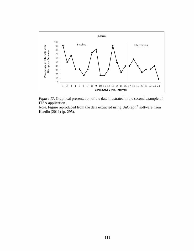
111


ITSA application.


Kazdin (2011) (p. 295).

112


ITSA application.


Kazdin (2011) (p. 295).

113


application.


Kazdin (2011) (p. 396).

114

CHAPTER 4

CONCLUSIONS

The goal of this dissertation was to address the scientific debate regarding the

most reliable and valid method of single-subject data evaluation in the applied

behavior analysis research field. This research conducted a head-to-head comparison

of the conclusions based on visual analysis and interrupted-times series analysis

(ITSA) using the same single-subject data.

Two independent studies were conducted, to examine the level of agreement

between visual analysis and ITSA. The first study was based on the graphical data

published in the Journal of Applied Behavior Analysis (2010). The second study was

based on graphical data obtained from the book titled “Single-Case research designs:

Methods for clinical and applied settings” by Alan E. Kazdin (2011).

In addition to a comparison of the conclusions based on visual and statistical

method, serial dependency of the data was also evaluated, as well as additional

statistical characteristics of single-subject experimental designs such as effect size and

sample size.

Overall findings for both studies show that ITSA can be successfully applied to at

least 95% of single-subject experiments with different sample sizes ranging from 8 to

136 observations and highly diverse study designs, ranging from the most basic AB

designs to designs with multiple phases and two or more types of interventions (e.g.

ABACABAC, ABCDEFBFEDC).

115

Evaluation of serial dependency revealed high lag-1 autocorrelations for most of

the evaluated data in both studies, including short time-series of less than 20

observations. These results confirm findings based on earlier studies showing that

serial dependency is a common property of single-subject data. The majority of first

order autocorrelations (62% and 67%, for study 1 and study 2 respectively) were

positive and at the moderate to high level (.41-.60 or >.60). The effect size estimates

were predominately large, with Cohen’s d ≥ 0.80 for 73% of time-series data in study

1 and 75% in study 2. The term 'clinical significance' can be viewed as analogous to a

large effect size. Statistical significance is typically viewed as a necessary but not

sufficient condition for clinical significance. Based on this interpretation, the effect

size estimates observed in this set of studies supports to the contention that graphical

methods focus mostly on clinically significant effect sizes.


an overall low level of agreement (Kappa = .14) in study 1 and moderate level of

agreement (Kappa = .44) in study 2.

The difference in the levels of agreement between the two studies could be driven

by the type of single-subject experimental designs presented in each source. It can be

expected that the Journal of Applied Behavior Analysis (2010) presents a more

representative sample of all single-subject studies recently conducted in the field of

applied behavior analysis. However, the graphical data presented in the textbook by

Kazdin (2011) is based on a non-representative sample of published single-subject

studies that were selected as instructional examples used for teaching visual analysis

methods. Therefore, the chosen single-subject experimental designs are largely based

116

on the most basic single-subject study designs with easily observable intervention

effects. Consequently, data based on intervention effects that present ideal or almost

ideal data patterns, such as with low variability, no trend in the data, and evident

intervention effects, ITSA was more likely to be in an agreement with visual analysis,

even for studies with small numbers of observations or experimental designs with

more than two phases (AB).

In conclusion, these findings show that ITSA can be broadly implemented in 95%

of applied behavior analysis research and can facilitate the evaluation of intervention

effects and additional statistical characteristics of the data, particularly when specific

characteristics of the single-subject data (e.g., slope, change in slope, etc.) limit the

reliability and validity of visual analysis. Overall, the two methods can be viewed as

complimentary and can be used concurrently, while retaining the benefits of both

methods, to advance the field and accumulate an evidence base over time.

Comparing Visual and Statistical Analysis in Single ...

Documents

Transcript of Comparing Visual and Statistical Analysis in Single ...