Comparing two proportions

SADC Course in Statistics

Comparing two proportions

(Session 14)

2To put your footer here go to View > Header and Footer

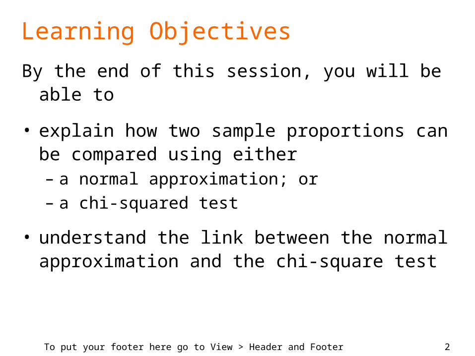
Learning Objectives

By the end of this session, you will be able to

• explain how two sample proportions can be compared using either – a normal approximation; or – a chi-squared test

• understand the link between the normal approximation and the chi-square test


Dealing with categorical data

In most of the previous sessions, the focus has been on quantitative measurements.

Many data variables collected in practice are however, categorical in nature, especially those emerging from surveys, e.g.

– gender of HH head (male/female)– level of education (none, primary,

secondary, tertiary)– whether of not HH has access to clean

water (yes/no)– failure of a crop (success/failure), etc.


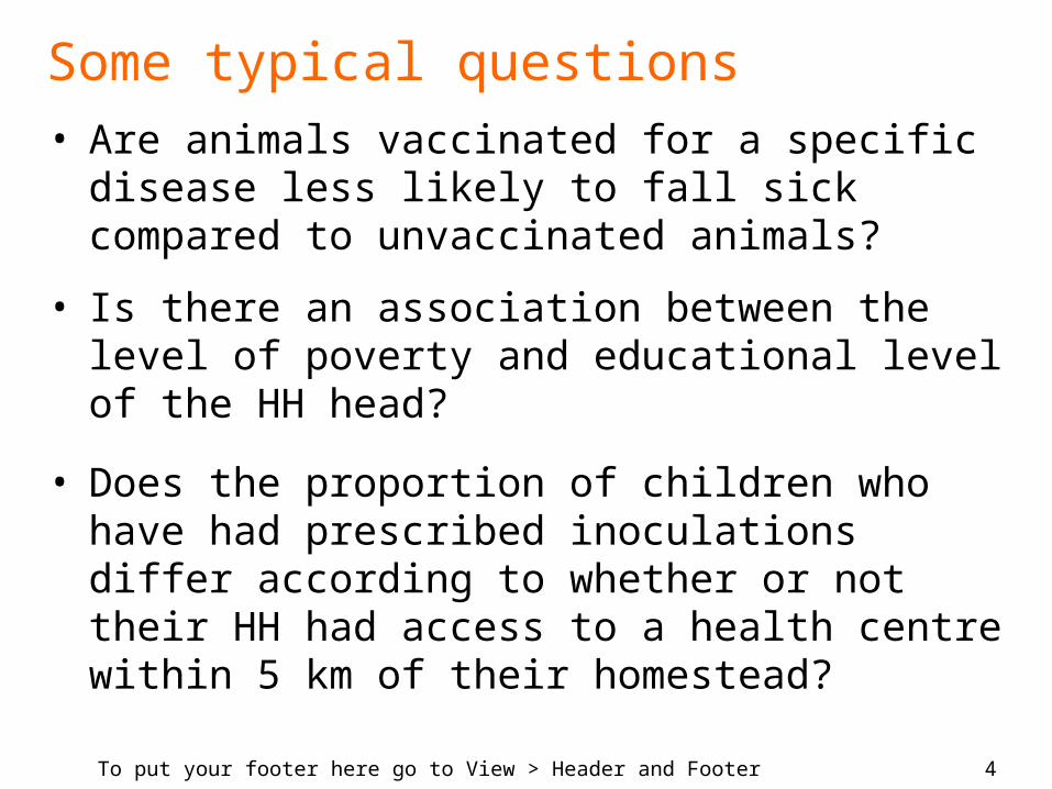
Some typical questions• Are animals vaccinated for a specific

disease less likely to fall sick compared to unvaccinated animals?

• Is there an association between the level of poverty and educational level of the HH head?

• Does the proportion of children who have had prescribed inoculations differ according to whether or not their HH had access to a health centre within 5 km of their homestead?


An example comparing proportions

In a long-term study on the relationship between smoking and mortality amongst males with cardiovascular problems, such individuals > 60 years were monitored.

After 6 years, it was found that 117 out of 1067 non-smokers group had died, while this was 54 out of 356 amongst smokers.

Is there evidence of a difference in death rates between smokers and non-smokers?


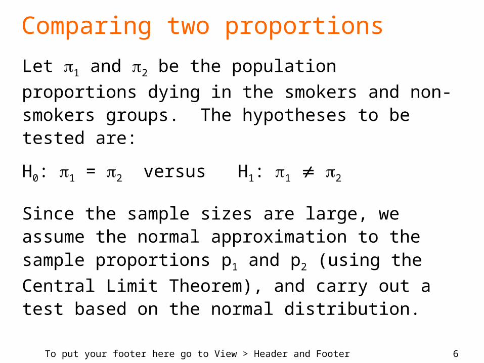
Comparing two proportions

Let 1 and 2 be the population proportions

dying in the smokers and non-smokers groups. The hypotheses to be tested are:

H0: 1 = 2 versus H1: 1 2

Since the sample sizes are large, we assume the normal approximation to the sample proportions p1 and p2 (using the Central Limit

Theorem), and carry out a test based on the normal distribution.


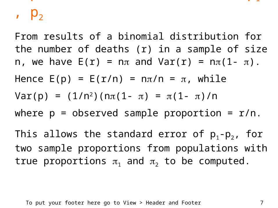
Expectation and variance of p1 , p2

From results of a binomial distribution for the number of deaths (r) in a sample of size n, we have E(r) = n and Var(r) = n(1- ).

Hence E(p) = E(r/n) = n/n = , while

Var(p) = (1/n2)(n(1- ) = (1- )/n

where p = observed sample proportion = r/n.

This allows the standard error of p1-p2, for two

sample proportions from populations with true proportions 1 and 2 to be computed.


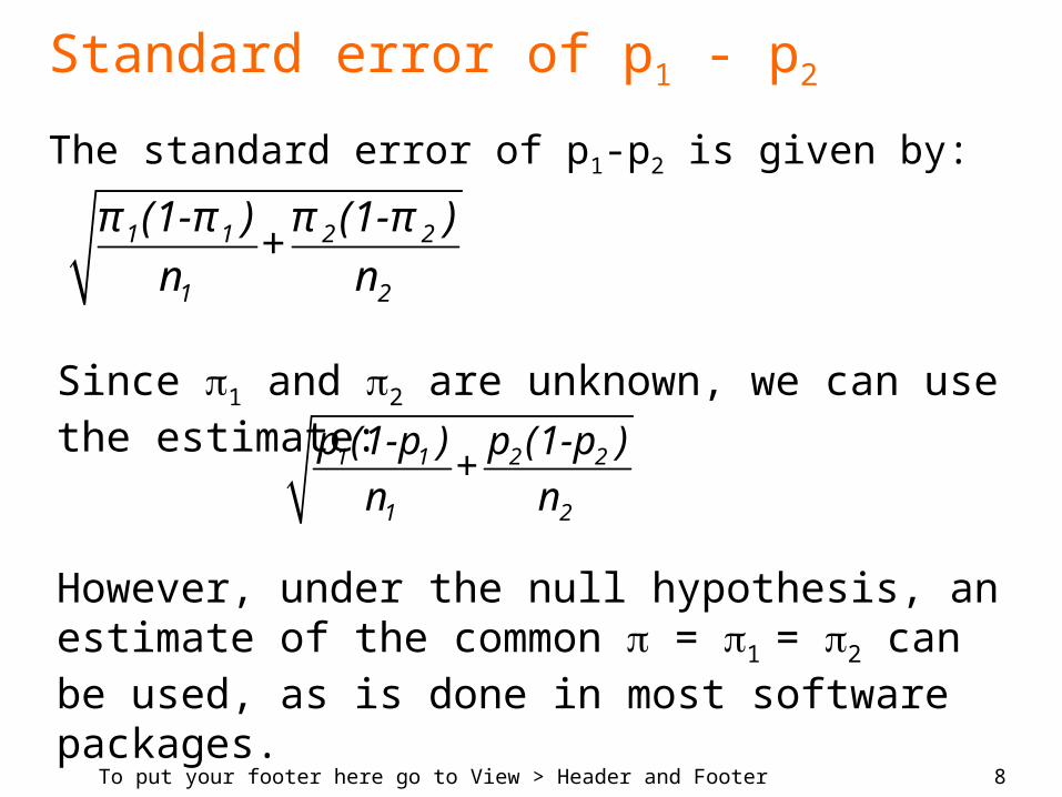
Standard error of p1 - p2

The standard error of p1-p2 is given by:

1 1 2 2

1 2

π (1-π ) π (1-π )+

n n

1 1 2 2

1 2

p (1-p ) p (1-p )+

n n

Since 1 and 2 are unknown, we can use the estimate:

However, under the null hypothesis, an estimate of the common = 1 = 2 can be used, as is done in most software packages.


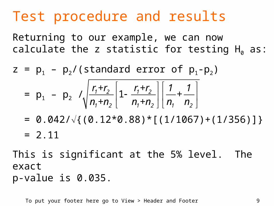
Test procedure and results

Returning to our example, we can now calculate the z statistic for testing H0 as:

z = p1 – p2/(standard error of p1-p2)

= p1 – p2 /

= 0.042/{(0.12*0.88)*[(1/1067)+(1/356)]}

= 2.11

This is significant at the 5% level. The exact p-value is 0.035.

11 2 1 2

1 2 1 2 1 2

r +r r +r 1 1+

n +n n +n n n


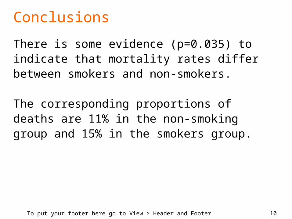
Conclusions

There is some evidence (p=0.035) to indicate that mortality rates differ between smokers and non-smokers.

The corresponding proportions of deaths are 11% in the non-smoking group and 15% in the smokers group.


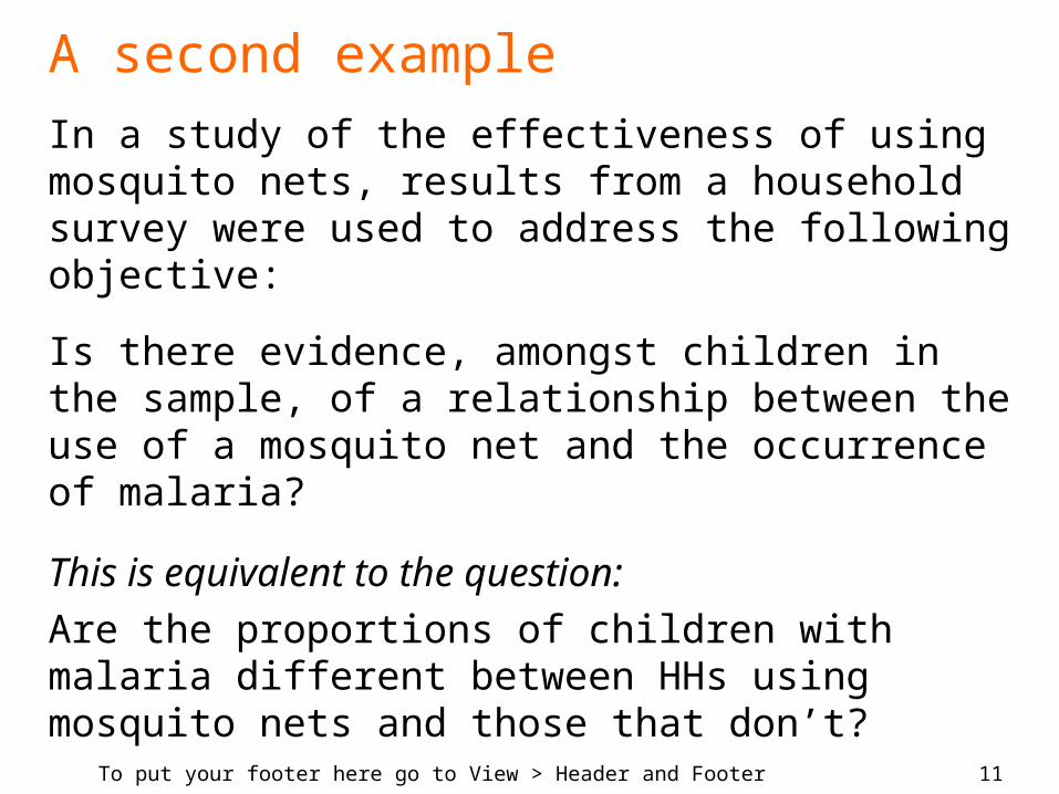
A second example

In a study of the effectiveness of using mosquito nets, results from a household survey were used to address the following objective:

Is there evidence, amongst children in the sample, of a relationship between the use of a mosquito net and the occurrence of malaria?

This is equivalent to the question:Are the proportions of children with malaria different between HHs using mosquito nets and those that don’t?


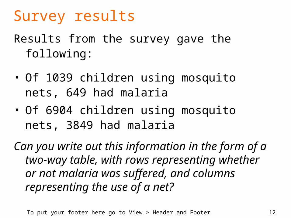
Survey results

Results from the survey gave the following:

• Of 1039 children using mosquito nets, 649 had malaria

• Of 6904 children using mosquito nets, 3849 had malaria

Can you write out this information in the form of a two-way table, with rows representing whether or not malaria was suffered, and columns representing the use of a net?


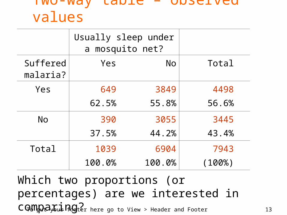
Two-way table – observed valuesUsually sleep under a

mosquito net?

Suffered malaria?

Yes No Total

Yes 649

62.5%

3849

55.8%

4498

56.6%

No 390

37.5%

3055

44.2%

3445

43.4%

Total 1039

100.0%

6904

100.0%

7943

(100%)

Which two proportions (or percentages) are we interested in comparing?


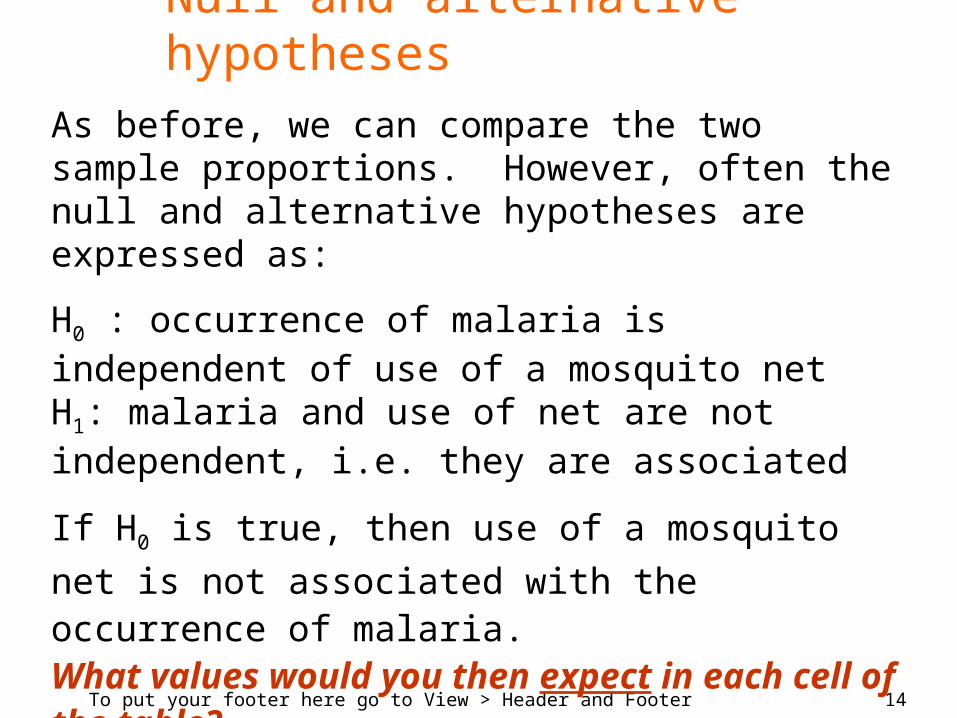
Null and alternative hypothesesAs before, we can compare the two sample proportions. However, often the null and alternative hypotheses are expressed as:

H0 : occurrence of malaria is independent of use of a mosquito netH1: malaria and use of net are not independent, i.e. they are associated

If H0 is true, then use of a mosquito net is not

associated with the occurrence of malaria.What values would you then expect in each cell of the table?


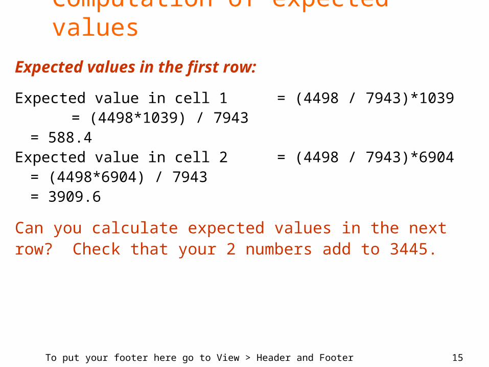
Expected values in the first row:

Expected value in cell 1 = (4498 / 7943)*1039 = (4498*1039) / 7943

= 588.4Expected value in cell 2 = (4498 / 7943)*6904

= (4498*6904) / 7943= 3909.6

Can you calculate expected values in the nextrow? Check that your 2 numbers add to 3445.

Computation of expected values


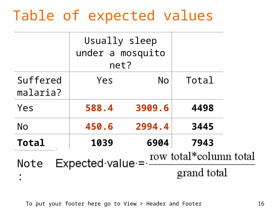
Usually sleep under a mosquito net?

Suffered malaria?

Yes No Total

Yes 588.4 3909.6 4498

No 450.6 2994.4 3445

Total 1039 6904 7943

Note:

Table of expected values


The chi-square test statistic

Here we test the null hypothesis using a chi-square test. The first step is to compute the chi-square (2) test statistic. The formula is:

Comparing this value with values of the 2 distribution with 1 d.f., shows the result is significant at the 1% level. We conclude there is strong evidence to reject the null hypothesis.

22

allcells

(O-E)X = = 16.57

E


What would have happened if we had done a z-test to compare the two proportions of children with malaria who use, and do not use a mosquito net?

The result would be an z-statistic = 4.07

This again leads to a highly significant p-value of 0.000. Note that the square of z above is 16.565. This is identical to the chi-square statistic. This is expected since theoretically, it is known that z2 =2 with 1 d.f. So the two tests are equivalent!

Comparison with z-test


We haven’t yet dealt with how best to present results of a chi-square test, and further interpretation of results of this last example.

We also have not discussed assumptions underlying the chi-square test and actions to take if assumptions fail.

These issues will be dealt with in the next two sessions.

Some final remarks


Some practical work follows…

Comparing two proportions

Documents

Transcript of Comparing two proportions