Comparing the Various Types of Multiple Regression

• Suppose we have the following hypothesis about some variables from the World95.sav data set:

• A country’s rate of male literacy (Y) is associated with a smaller rate of annual population increase (X1), a greater gross domestic product (X2), and a larger percentage of people living in cities (X3)

• First let’s look at the intercorrelation among these four variables

• What we hope to find is that each of the three predictors has at least a moderate correlation with the Y variable, male literacy, but are not too highly intercorrelated themselves (avoiding multicollinearity)

• Let’s check this out by obtaining the zero-order correlations

Starting with the Zero-order Correlation Matrix

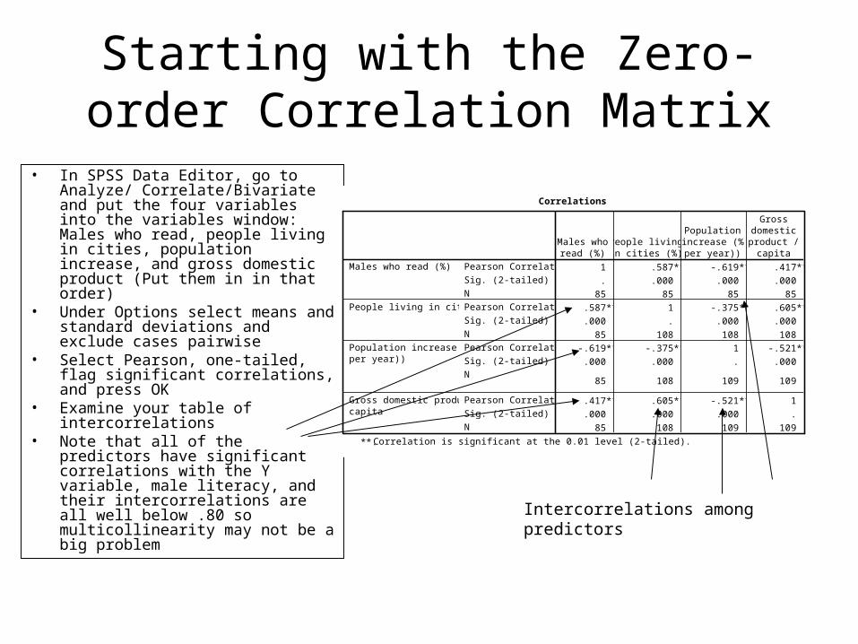
• In SPSS Data Editor, go to Analyze/ Correlate/Bivariate and put the four variables into the variables window: Males who read, people living in cities, population increase, and gross domestic product (Put them in in that order)

• Under Options select means and standard deviations and exclude cases pairwise

• Select Pearson, one-tailed, flag significant correlations, and press OK

• Examine your table of intercorrelations

• Note that all of the predictors have significant correlations with the Y variable, male literacy, and their intercorrelations are all well below .80 so multicollinearity may not be a big problem

Correlations

1 .587** -.619** .417**

. .000 .000 .000

85 85 85 85

.587** 1 -.375** .605**

.000 . .000 .000

85 108 108 108

-.619** -.375** 1 -.521**

.000 .000 . .000

85 108 109 109

.417** .605** -.521** 1

.000 .000 .000 .

85 108 109 109

Pearson Correlation

Sig. (2-tailed)

N

Pearson Correlation

Sig. (2-tailed)

N

Pearson Correlation

Sig. (2-tailed)

N

Pearson Correlation

Sig. (2-tailed)

N

Males who read (%)

People living in cities (%)

Population increase (%per year))

Gross domestic product /capita

Males whoread (%)

People livingin cities (%)

Populationincrease (%per year))

Grossdomesticproduct /

capita

Correlation is significant at the 0.01 level (2-tailed).**.

Intercorrelations among predictors

SPSS Setup for Simultaneous Multiple Regression on Three Predictor

Variables• Now let’s run a standard (simultaneous) multiple

regression of Y (male literacy) on the three predictor variables– In Data Editor go to Analyze/ Regression/ Linear and click the Reset

button– Put Male Literacy into the Dependent box– Put Population Increase, People Living in Cities, and Gross Domestic

Product into the Independents box– Under Statistics, select Estimates, Confidence Intervals, Model Fit, R

squared change, Descriptives, Part and Partial Correlation, Collinearity Diagnostics and click Continue

– Under Options, check Include Constant in the Equation, click Continue and then OK

– Under Method, select enter. This will enter all of the variables into the regression equation

• Compare your output to the next several slides

Variables Entered/Removed Table

• First look at the table of variables entered– You will see that all three of the predictor variables have

been included in the regression equation

Model Summary, Simultaneous Multiple Regression

• Next look at the Model Summary. You will see that– The multiple correlation (R) between male literacy and the three

predictors is strong: .764, – The combination of the three predictors accounts for nearly 60% of the

variation in male literacy (R square): .583– The regression equation is significant (F 3, 81) = 37.783, p < .001.

This information is also contained in the ANOVA table

Model Summary

.764a .583 .568 13.441 .583 37.783 3 81 .000Model1

R R SquareAdjustedR Square

Std. Error ofthe Estimate

R SquareChange F Change df1 df2 Sig. F Change

Change Statistics

Predictors: (Constant), Gross domestic product / capita, Population increase (% per year)), People living in cities (%)a. ANOVAb

20478.670 3 6826.223 37.783 .000a

14634.107 81 180.668

35112.776 84

Regression

Residual

Total

Model1

Sum ofSquares df Mean Square F Sig.

Predictors: (Constant), Gross domestic product / capita, Population increase (%per year)), People living in cities (%)

a.

Dependent Variable: Males who read (%)b.

Listwise Exclusion:Exclude a case if it is missingdata on any one of the variables-more typical for multivariatePairwise-typical for bivariate-exclude cases if they’re missing x or y

Regression Weights, Simultaneous Multiple Regression

• Now let’s look at the regression weights (the beta coefficients) (I have divided this table into two halves; this is the left side below). From this table you will learn that

• Two of the predictors have significant standardized regression weights (population increase, Beta=-.517, t = -6.698, p < .000; people living in cities, Beta = .493, t = 5.539, p <.001): that is, each of the two is a significant contributor to predicting male literacy

• GDP does not appear to add unique predictive power when the effects of the other predictors are held constant (Beta = -.063, t = -.676, p = .501)

• The sign of the regression weights is in the predicted direction, with male literacy being positively associated with % people living in cities and GDP, but negatively associated with % annual population increases

Multicollinearity Statistics

• So far you have found partial support but not full support for your hypothesis: given this analysis it would have to be revised to leave out GDP as a predictor. What you appear to have found is that Male literacy (in standard scores) = -.517 (Population increase in standard units) + .493 (People living in cities in standard units) (not quite; need to rerun it without GDP)

• But not so fast! First let’s check to make sure we don’t have any multicollinearity issues. Below are the collinearity statistics from the coefficients table. Recall that for multicollinearity to be a problem tolerance had to approach zero and VIF approach 10. So everthing below looks OK and you can report what that you have found modified support for your hypothesis, minus the effect of GDP

Hierarchical Multiple Regression

• Now let’s analyze the same data and ask the same question with a different method of multiple regression

• This time we will try a hierachical model where we will enter the variables based on some external criterion of our own, like a theoretical model

• Based on our theory of why men read, we have decided to first enter the variable people living in cities, then annual population increase, then GDP

• We are going to make some changes to the way we set up the analysis

SPSS Setup for Hierarchical Multiple Regression

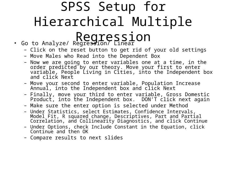
• Go to Analyze/ Regression/ Linear– Click on the reset button to get rid of your old settings– Move Males who Read into the Dependent Box– Now we are going to enter variables one at a time, in the order predicted

by our theory. Move your first to enter variable, People Living in Cities, into the Independent box and click Next

– Move your second to enter variable, Population Increase Annual, into the Independent box and click Next

– Finally, move your third to enter variable, Gross Domestic Product, into the Independent box. DON’T click next again

– Make sure the enter option is selected under Method– Under Statistics, select Estimates, Confidence Intervals, Model Fit, R

squared change, Descriptives, Part and Partial Correlation, and Collinearity Diagnostics, and click Continue

– Under Options, check Include Constant in the Equation, click Continue and then OK

– Compare results to next slides

Entered/Removed Table for Hierarchical Multiple Regression

• The box called Variables Entered/ Removed gives you a summary of what’s in the model and the information about the order in which it was entered or removed. Here you have all three variables entered, and you are going to be comparing three different “models” or regression equations; one with only people living in cities as a predictor, a two-variable model with people living in cities and population increase % annual as predictors, and finally a model with all three of the predictors combined

Variables Entered/Removedb

Peopleliving incities (%)

a . Enter

Populationincrease(% peryear))

a. Enter

Grossdomesticproduct /capita

a. Enter

Model1

2

3

VariablesEntered

VariablesRemoved Method

All requested variables entered.a.

Dependent Variable: Males who read (%)b.

Model Summary for Hierarchical Multiple Regression

• Next we are going to look at our model summary, which compares each of the three models (one, two, or three predictors). Note that for model 1, with only the people living in cities predictor, r is the same as the zero-order correlation between male literacy and people living in cities. But the associated R square is significant (i.e., the regression equation is better than using the mean of Y as a predictor) at F (1,83) = 43.668, p < .001. Model 2, with two of the three predictors, is even better, with an r of .762 and an R square of .581 of the variance accounted for. This change in R square is significant (F (1, 82) = 46.198, p<.001), indicating that the second predictor, population increase annual %, added significantly to the regression equation after the first predictor had done its work. But the third predictor, GDP, came up short. It only increased R square by a tiny bit, from .581 to .583, and the change in R square was not significant (F (1,81) = .457, n.s)

Model Summary

.587a .345 .337 16.649 .345 43.668 1 83 .000

.762b .581 .571 13.397 .236 46.198 1 82 .000

.764c .583 .568 13.441 .002 .457 1 81 .501

Model1

2

3

R R SquareAdjustedR Square

Std. Error ofthe Estimate

R SquareChange F Change df1 df2 Sig. F Change

Change Statistics

Predictors: (Constant), People living in cities (%)a.

Predictors: (Constant), People living in cities (%), Population increase (% per year))b.

Predictors: (Constant), People living in cities (%), Population increase (% per year)), Gross domestic product / capitac.

ANOVA Tests, Hierarchical Multiple Regression

• Our ANOVA table gives us the significance of each of the three models (one predictor, two predictors, three predictors) and we see that the F is largest for the two-predictor model). (These Fs are for the overall predictive effect and are different than the F for the amount of change we get when adding in an additional variable as on the previous slide.) The F for the three-variable equation (37.783)is also equal to the final F we got in the standard (simultaneous) method when we entered all of the variables at once. So we have all the evidence we need to toss out the third variable as a predictor, unless we have some reason to assume that GDP “causes” one of the other predictors

ANOVAd

12104.898 1 12104.898 43.668 .000a

23007.879 83 277.203

35112.776 84

20396.129 2 10198.065 56.823 .000b

14716.647 82 179.471

35112.776 84

20478.670 3 6826.223 37.783 .000c

14634.107 81 180.668

35112.776 84

Regression

Residual

Total

Regression

Residual

Total

Regression

Residual

Total

Model1

2

3

Sum ofSquares df Mean Square F Sig.

Predictors: (Constant), People living in cities (%)a.

Predictors: (Constant), People living in cities (%), Population increase (% per year))b.

Predictors: (Constant), People living in cities (%), Population increase (% per year)),Gross domestic product / capita

c.

Dependent Variable: Males who read (%)d.

Regression Coefficients, Hierarchal Multiple Regression

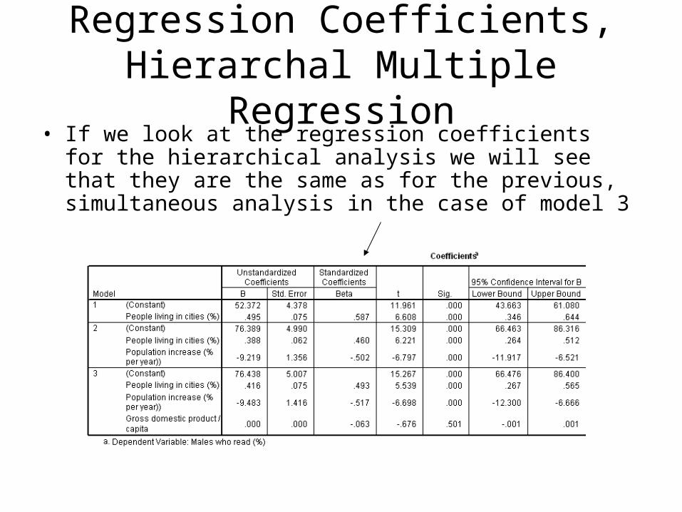
• If we look at the regression coefficients for the hierarchical analysis we will see that they are the same as for the previous, simultaneous analysis in the case of model 3

Writing up your Results

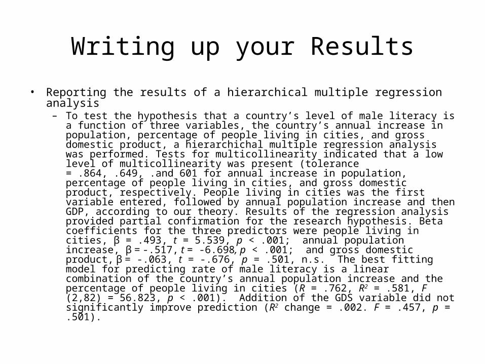
• Reporting the results of a hierarchical multiple regression analysis– To test the hypothesis that a country’s level of male literacy is a function of three

variables, the country’s annual increase in population, percentage of people living in cities, and gross domestic product, a hierarchichal multiple regression analysis was performed. Tests for multicollinearity indicated that a low level of multicollinearity was present (tolerance = .864, .649, .and 601 for annual increase in population, percentage of people living in cities, and gross domestic product, respectively. People living in cities was the first variable entered, followed by annual population increase and then GDP, according to our theory. Results of the regression analysis provided partial confirmation for the research hypothesis. Beta coefficients for the three predictors were people living in cities, β = .493, t = 5.539, p < .001; annual population increase, β = -.517, t = -6.698, p < .001; and gross domestic product, β = -.063, t = -.676, p = .501, n.s. The best fitting model for predicting rate of male literacy is a linear combination of the country’s annual population increase and the percentage of people living in cities (R = .762, R2 = .581, F (2,82) = 56.823, p < .001). Addition of the GDS variable did not significantly improve prediction (R2 change = .002. F = .457, p = .501).

Stepwise Multiple Regression• Finally, let’s look at a stepwise multiple regression

– In SPSS Data Editor, go to Analyze/ Regression/ Linear– Click the reset button– Put Male Literacy into the Dependent box– Put Population Increase, People Living in Cities, and Gross Domestic

Product into the Independents box– Under Method, select Stepwise– Under Statistics, select Estimates, Confidence Intervals, Model Fit, R

squared change, Descriptives, Part and Partial Correlation, and Collinearity Diagnostics, and click Continue

– Under Options, check Include Constant in the Equation, and under Stepping Method criteria select “use probability of F” and set F to enter a variable to .005 and and F to remove a variable to .01. We are making this alpha adjustment to control the overall error rate which may increase because of the more frequent probability testing that is done in stepwise regression. Click Continue and then OK

Variables Entered/Removed Table for Stepwise Multiple Regression

• The table of variables entered and removed shows that only the first two predictors, population increase annual and people living in cities were ever entered in the analysis. The third variable, GDP, evidently did not pass the entry test of an F with associated probability level of .005

Variables Entered/Removeda

Populationincrease(% peryear))

.

Stepwise(Criteria:Probability-of-F-to-enter<= .005,Probability-of-F-to-remove >= .010).

Peopleliving incities (%)

.

Stepwise(Criteria:Probability-of-F-to-enter<= .005,Probability-of-F-to-remove >= .010).

Model1

2

VariablesEntered

VariablesRemoved Method

Dependent Variable: Males who read (%)a.

Model Summary for Stepwise Multiple Regression

• With our third variable out of the picture, the model summary looks a little different because the effects of the third variable have been removed both from the first two and their relationship to the dependent variable. The increase in R square with model 1 (only population increase) is significant as well as the further increase in R square with the addition of the second variable (Model 2)

Model Summary

.619a .383 .376 16.155 .383 51.538 1 83 .000

.762b .581 .571 13.397 .198 38.699 1 82 .000

Model1

2

R R SquareAdjustedR Square

Std. Error ofthe Estimate

R SquareChange F Change df1 df2 Sig. F Change

Change Statistics

Predictors: (Constant), Population increase (% per year))a.

Predictors: (Constant), Population increase (% per year)), People living in cities (%)b.

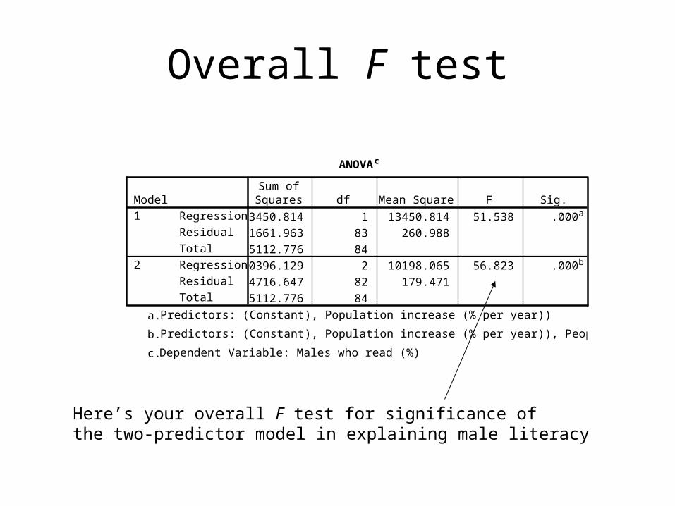
Overall F test

ANOVAc

13450.814 1 13450.814 51.538 .000a

21661.963 83 260.988

35112.776 84

20396.129 2 10198.065 56.823 .000b

14716.647 82 179.471

35112.776 84

Regression

Residual

Total

Regression

Residual

Total

Model1

2

Sum ofSquares df Mean Square F Sig.

Predictors: (Constant), Population increase (% per year))a.

Predictors: (Constant), Population increase (% per year)), People living in cities (%)b.

Dependent Variable: Males who read (%)c.

Here’s your overall F test for significance ofthe two-predictor model in explaining male literacy

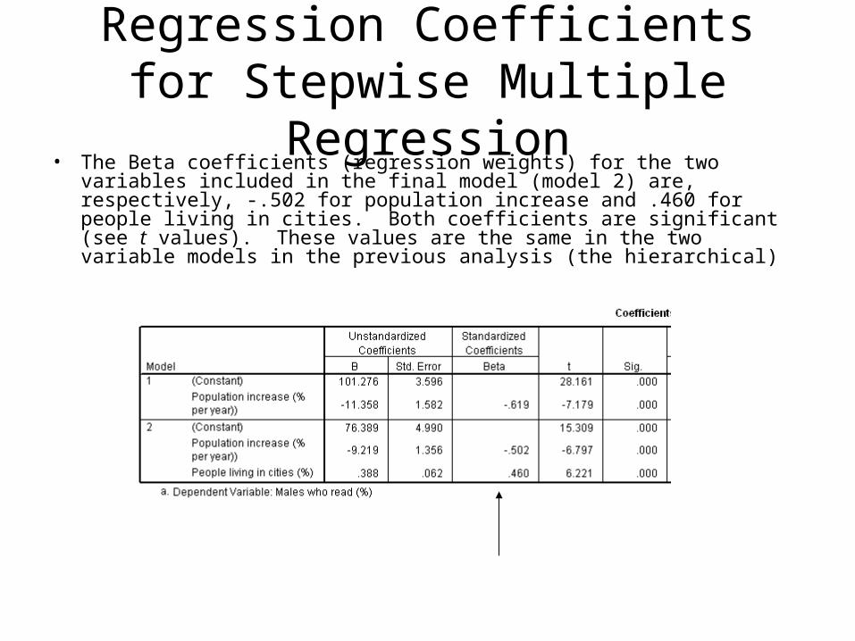
Regression Coefficients for Stepwise Multiple Regression

• The Beta coefficients (regression weights) for the two variables included in the final model (model 2) are, respectively, -.502 for population increase and .460 for people living in cities. Both coefficients are significant (see t values). These values are the same in the two variable models in the previous analysis (the hierarchical)

Sample Writeup of a Step-Wise Multiple Regression

– To test the hypothesis that a country’s level of male literacy is a function of three variables, the country’s annual increase in population, percentage of people living in cities, and gross domestic product, a stepwise multiple regression analysis was performed. Levels of F to enter and F to remove were set to correspond to p levels of .005 and .01, respectively, to adjust for familywise alpha error rates associated with multiple significance tests. Tests for multicollinearity indicated that a low level of multicollinearity was present (tolerance = .864, .649, .and 601 for annual increase in population, percentage of people living in cities, and gross domestic product, respectively. Results of the stepwise regression analysis provided partial confirmation for the research hypothesis: rate of male literacy is a linear function of the country’s annual population increase and the percentage of people living in cities (R = .762, R2 = .581). The overall F for the two-variable model was 56.823, df = 2, 82, p < .001. Standardized beta weights were -.502 for annual population increase and .460 for percentage of people living in cities.

Variable Exclusion in Stepwise Regression

• As an example of stepwise multiple regression with a larger number of predictor variables, I regressed daily calorie intake on these six predictors: Population in thousands; Number of people / sq. kilometer; People living in cities (%); People who read (%); Population increase (% per year; and Gross domestic product. The final model consisted of only two of the variables, GDP and Cities. The rest were excluded because they did not have a low enough p value (.005) to enter, due to the fact that their partial correlation with the dependent variable, Y (daily caloric intake), with the effects of the other predictors held constant, was not significant, even though their zero order correlation with the dependent variable, Y, may have been.

• Now see if you can duplicate this analysis.

In the final model, only GDP and people living in cities were retained

Points to Remember about Multiple Regression

• To sum up– In doing a regression, first obtain a matrix of the zero-order

correlations among the candidate predictor variables and look for multicollinearity problems (variables too highly correlated)

– Consider whether your theory would dictate that the variables be entered in any particular order

– If there is no theory to guide you, consider if you want to enter all the variables at once or let empirical criteria like a fixed probability level determine if they are allowed to enter the equation

– Adjust the significance level to make the alpha levels smaller on F to enter and remove especially if you have a lot of variables