Comparing One or Two Means Using the t-Test
30
3 Comparing One or Two Means Using the t-Test T he bread and butter of statistical data analysis is the Student’s t-test. It was named after a statistician who called himself Student but whose real name was William Gossett. As an employee of Guinness Brewery in Dublin, Ireland, he tackled a number of practical statistical problems related to the operation of the brewery. Since he was discouraged from publishing under his own name, he adopted the Student moniker. Because of Gossett’s work, today’s researchers have in their toolbox what is probably the most commonly performed statistical procedure, the t-test. The most typical use of this test is to compare means, which is the focus of the discussion in this chapter. Unfortunately, because this test is easy to use, it is also easily misused. In this chapter, you will learn when, why, and how to appropriately per- form a t-test and how to present your results. There are three types of t-tests that will be discussed in this chapter. These are the 1. One-sample t-test, which is used to compare a single mean to a fixed number or “gold standard” 2. Two-sample t-test, which is used to compare two population means based on independent samples from the two populations or groups 3. Paired t-test, which is used to compare two means based on samples that are paired in some way 47 03-Elliott-4987.qxd 7/18/2006 3:43 PM Page 47
Transcript of Comparing One or Two Means Using the t-Test
3Comparing One or TwoMeans Using the t-Test
The bread and butter of statistical data analysis is the Student’s t-test.It was named after a statistician who called himself Student but whose
real name was William Gossett. As an employee of Guinness Brewery inDublin, Ireland, he tackled a number of practical statistical problems relatedto the operation of the brewery. Since he was discouraged from publishingunder his own name, he adopted the Student moniker.
Because of Gossett’s work, today’s researchers have in their toolbox whatis probably the most commonly performed statistical procedure, the t-test.The most typical use of this test is to compare means, which is the focus ofthe discussion in this chapter. Unfortunately, because this test is easy to use,it is also easily misused.
In this chapter, you will learn when, why, and how to appropriately per-form a t-test and how to present your results. There are three types of t-teststhat will be discussed in this chapter. These are the
1. One-sample t-test, which is used to compare a single mean to a fixed numberor “gold standard”
2. Two-sample t-test, which is used to compare two population means based onindependent samples from the two populations or groups
3. Paired t-test, which is used to compare two means based on samples that arepaired in some way
47
03-Elliott-4987.qxd 7/18/2006 3:43 PM Page 47
These three types of t-tests are discussed along with advice concerningthe conditions under which each of these types is appropriate. Examples aregiven that illustrate how to perform these three types of t-tests using SPSSsoftware. The first type of t-test considered is the simplest.
One-Sample t-Test
The one-sample t-test is used for comparing sample results with a knownvalue. Specifically, in this type of test, a single sample is collected, and theresulting sample mean is compared with a value of interest, sometimes a“gold standard,” that is not based on the current sample. For example, thisspecified value might be
• The weight indicated on a can of vegetables• The advertised breaking strength of a type of steel pipe• Government specification on the percentage of fruit juice that must be in a
drink before it can be advertised as “fruit juice”
The purpose of the one-sample t-test is to determine whether there is suffi-cient evidence to conclude that the mean of the population from which thesample is taken is different from the specified value.
Related to the one-sample t-test is a confidence interval on the mean.The confidence interval is usually applied when you are not testing against aspecified value of the population mean but instead want to know a range ofplausible values of the unknown mean of the population from which thesample was selected.
Appropriate Applications for a One-Sample t-Test
The following are examples of situations in which a one-sample t-testwould be appropriate:
• Does the average volume of liquid in filled soft drink bottles match the12 ounces advertised on the label?
• Is the mean weight loss for men ages 50 to 60 years, who are given a brochureand training describing a low-carbohydrate diet, more than 5 pounds after3 months?
• Based on a random sample of 200 students, can we conclude that the averageSAT score this year is lower than the national average from 3 years ago?
Design Considerations for a One-Sample t-Test
The key assumption underlying the one-sample t-test is that the popula-tion from which the sample is selected is normal. However, this assumption
48——Statistical Analysis Quick Reference Guidebook
03-Elliott-4987.qxd 7/18/2006 3:43 PM Page 48

is rarely if ever precisely true in practice, so it is important to know howconcerned you should be about apparent nonnormality in your data. Thefollowing are rules of thumb (Moore & McCabe, 2006):
• If the sample size is small (less than 15), then you should not use theone-sample t-test if the data are clearly skewed or if outliers are present.
• If the sample size is moderate (at least 15), then the one-sample t-test can besafely used except when there are severe outliers.
• If the sample size is large (at least 40), then the one-sample t-test can be safelyused without regard to skewness or outliers.
You will see variations of these rules throughout the literature. The lasttwo rules above are based on the central limit theorem, which says thatwhen sample size is moderately large, the sample mean is approximately nor-mally distributed even when the original population is nonnormal.
Hypotheses for a One-Sample t-Test
When performing a one-sample t-test, you may or may not have a pre-conceived assumption about the direction of your findings. Depending on thedesign of your study, you may decide to perform a one- or two-tailed test.
Two-Tailed t-Tests
The basic hypotheses for the one-sample t-test are as follows, whereµ denotes the mean of the population from which the sample was selected,and µ0 denotes the hypothesized value of this mean. It should be reiteratedthat µ0 is a value that does not depend on the current sample.
H0: µ = µ0 (in words: the population mean is equal to the hypothesized value µ0).
Ha: µ ≠ µ0 (the population mean is not equal to µ0).
One-Tailed t-Tests
If you are only interested in rejecting the null hypothesis if the populationmean differs from the hypothesized value in a direction of interest, you maywant to use a one-tailed (sometimes called a one-sided) test. If, for example,you want to reject the null hypothesis only if there is sufficient evidence thatthe mean is larger than the value hypothesized under the null (i.e., µ0), thehypotheses become the following:
H0: µ = µ0 (the population mean is equal to the hypothesized value µ0).
Ha: µ > µ0 (the population mean is greater than µ0).
Comparing One or Two Means Using the t-Test——49
03-Elliott-4987.qxd 7/18/2006 3:43 PM Page 49

Analogous hypotheses could be specified for the case in which you wantto reject H0 only if there is sufficient evidence that the population mean isless than µ0.
SPSS always reports a two-tailed p-value, so you should modify thereported p-value to fit a one-tailed test by dividing it by 2 if your resultsare consistent with the direction specified in the alternative hypothesis. Formore discussion of the issues of one- and two-sample tests, see the section“Hypotheses for a Two-Sample t-Test” in this chapter.
EXAMPLE 3.1: One-Sample t-Test
Describing the Problem
A certain bolt is designed to be 4 inches in length. The lengths of a ran-dom sample of 15 bolts are shown in Figure 3.1.
50——Statistical Analysis Quick Reference Guidebook
Figure 3.1 The Bolt Data
Since the sample size is small (N = 15), we need to examine the normal-ity of the data before proceeding to the t-test. In Figure 3.2, we show theboxplot of the length data from which it can be seen that the data arereasonably symmetric, and thus the t-test should be an appropriate test.
03-Elliott-4987.qxd 7/18/2006 3:43 PM Page 50
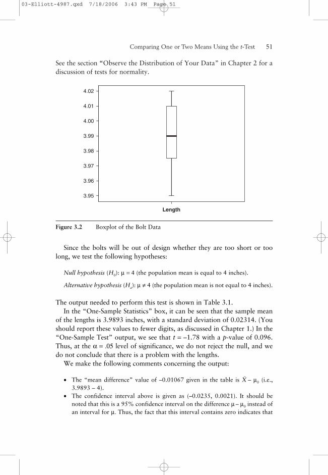
See the section “Observe the Distribution of Your Data” in Chapter 2 for adiscussion of tests for normality.
Comparing One or Two Means Using the t-Test——51
Length
4.02
4.01
4.00
3.99
3.98
3.97
3.96
3.95
Figure 3.2 Boxplot of the Bolt Data
Since the bolts will be out of design whether they are too short or toolong, we test the following hypotheses:
Null hypothesis (H0): µ = 4 (the population mean is equal to 4 inches).
Alternative hypothesis (Ha): µ ≠ 4 (the population mean is not equal to 4 inches).
The output needed to perform this test is shown in Table 3.1.In the “One-Sample Statistics” box, it can be seen that the sample mean
of the lengths is 3.9893 inches, with a standard deviation of 0.02314. (Youshould report these values to fewer digits, as discussed in Chapter 1.) In the“One-Sample Test” output, we see that t = –1.78 with a p-value of 0.096.Thus, at the α = .05 level of significance, we do not reject the null, and wedo not conclude that there is a problem with the lengths.
We make the following comments concerning the output:
• The “mean difference” value of –0.01067 given in the table is X–
– µ0 (i.e.,3.9893 – 4).
• The confidence interval above is given as (–0.0235, 0.0021). It should benoted that this is a 95% confidence interval on the difference µ – µ0 instead ofan interval for µ. Thus, the fact that this interval contains zero indicates that
03-Elliott-4987.qxd 7/18/2006 3:43 PM Page 51
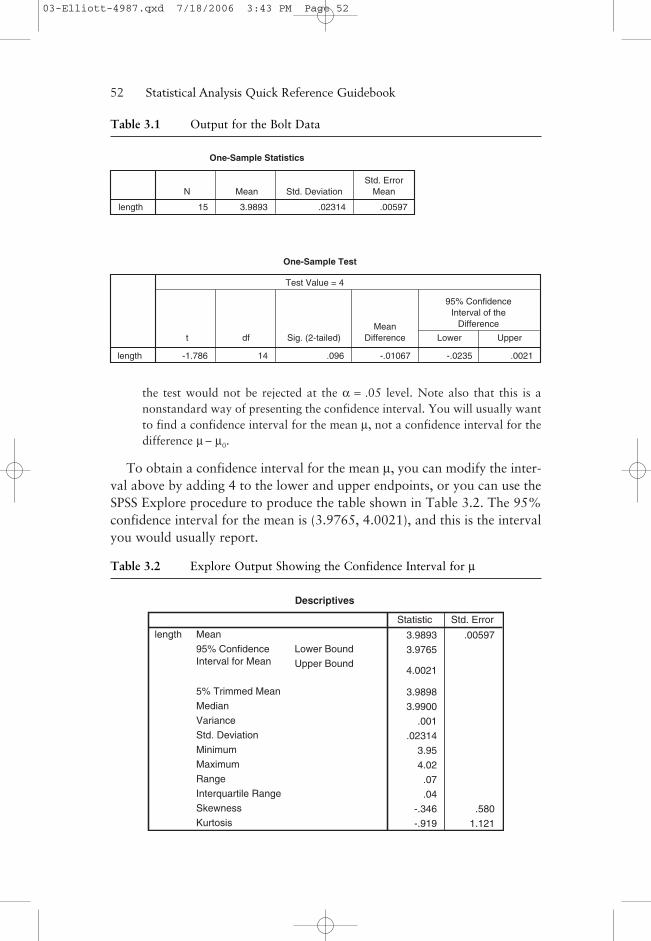
the test would not be rejected at the α = .05 level. Note also that this is anonstandard way of presenting the confidence interval. You will usually wantto find a confidence interval for the mean µ, not a confidence interval for thedifference µ – µ0.
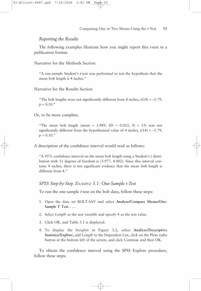
To obtain a confidence interval for the mean µ, you can modify the inter-val above by adding 4 to the lower and upper endpoints, or you can use theSPSS Explore procedure to produce the table shown in Table 3.2. The 95%confidence interval for the mean is (3.9765, 4.0021), and this is the intervalyou would usually report.
52——Statistical Analysis Quick Reference Guidebook
Table 3.1 Output for the Bolt Data
One-Sample Statistics
Mean Std. DeviationStd. Error
Mean
.00597.023143.9893
N
15length
One-Sample Test
length
t
-1.786
df
14
Sig. (2-tailed)
.096
MeanDifference
-.01067 -.0235
Lower
.0021
Upper
95% ConfidenceInterval of the
Difference
Test Value = 4
Table 3.2 Explore Output Showing the Confidence Interval for µ
Descriptives
3.9893 .00597
3.9765
4.0021
3.9898
3.9900
.001
.02314
3.95
4.02
.07
.04
-.346 .580
-.919 1.121
Mean
Lower Bound
Upper Bound
95% ConfidenceInterval for Mean
5% Trimmed Mean
Median
Variance
Std. Deviation
Minimum
Maximum
Range
Interquartile Range
Skewness
Kurtosis
length
Statistic Std. Error
03-Elliott-4987.qxd 7/18/2006 3:43 PM Page 52
Reporting the Results
The following examples illustrate how you might report this t-test in apublication format.
Narrative for the Methods Section
“A one-sample Student’s t-test was performed to test the hypothesis that themean bolt length is 4 inches.”
Narrative for the Results Section
“The bolt lengths were not significantly different from 4 inches, t(14) = –1.79,p = 0.10.”
Or, to be more complete,
“The mean bolt length (mean = 3.989, SD = 0.023, N = 15) was notsignificantly different from the hypothesized value of 4 inches, t(14) = –1.79,p = 0.10.”
A description of the confidence interval would read as follows:
“A 95% confidence interval on the mean bolt length using a Student’s t distri-bution with 11 degrees of freedom is (3.977, 4.002). Since this interval con-tains 4 inches, there is not significant evidence that the mean bolt length isdifferent from 4.”
SPSS Step-by-Step. EXAMPLE 3.1: One-Sample t-Test
To run the one-sample t-test on the bolt data, follow these steps:
1. Open the data set BOLT.SAV and select Analyze/Compare Means/One-Sample T Test. . . .
2. Select Length as the test variable and specify 4 as the test value.
3. Click OK, and Table 3.1 is displayed.
4. To display the boxplot in Figure 3.2, select Analyze/DescriptiveStatistics/Explore, add Length to the Dependent List, click on the Plots radiobutton at the bottom left of the screen, and click Continue and then OK.
To obtain the confidence interval using the SPSS Explore procedure,follow these steps:
Comparing One or Two Means Using the t-Test——53
03-Elliott-4987.qxd 7/18/2006 3:43 PM Page 53

1. Open the data set BOLT.SAV and select Analyze/Descriptive Statistics/Explore. . . .
2. Add Length to the Dependent List.
3. Click OK, and the output includes the information in Table 3.2.
Two-Sample t-Test
The two-sample (independent groups) t-test is used to determine whetherthe unknown means of two populations are different from each other basedon independent samples from each population. If the two-sample means aresufficiently different from each other, then the population means aredeclared to be different. A related test, the paired t-test, to be discussed inthe next section, is used to compare two population means using samplesthat are paired in some way.
The samples for a two-sample t-test can be obtained from a single popu-lation that has been randomly divided into two subgroups, with each sub-group subjected to one of two treatments (e.g., two medications) or fromtwo separate populations (e.g., male and female). In either case, for the two-sample t-test to be valid, it is necessary that the two samples are independent(i.e., unrelated to each other).
Appropriate Applications for a Two-Sample t-Test
In each of the following examples, the two-sample (independent group)t-test is used to determine whether the population means of the two groupsare different.
• How Can My Flour Make More Dough? Distributors often pay extra to haveproducts placed in prime locations in grocery stores. The manufacturer of anew brand of whole-grain flour wants to determine if placing the product onthe top shelf or on the eye-level shelf produces better sales. From 40 grocerystores, he randomly chooses 20 for top-shelf placement and 20 for eye-levelplacement. After a period of 30 days, he compares average sales from the twoplacements.
• What’s the Smart Way to Teach Economics? A university is offering twosections of a microeconomics course during the fall semester: (1) meeting oncea week with taped lessons provided on a CD and (2) having three sessions aweek using standard lectures by the same professor. Students are randomlyplaced into one of the two sections at the time of registration. Using resultsfrom a standardized final exam, the researcher compares mean differencesbetween the learning obtained in the two types of classes.
54——Statistical Analysis Quick Reference Guidebook
03-Elliott-4987.qxd 7/18/2006 3:43 PM Page 54

• Are Males and Females Different? It is known that males and females oftendiffer in their reactions to certain drugs. As a part of the development ofa new antiseizure medication, a standard dose is given to 20 males and 20females. Periodic measurements are made to determine the time it takes untila desired level of drug is present in the blood for each subject. The researcherwants to determine whether there is a gender difference in the average speedat which the drug is assimilated into the blood system.
Design Considerations for a Two-Sample t-Test
The characteristics of the t-tests in the above examples are the following:
A Two-Sample t-Test Compares Means
In an experiment designed to use the two-sample t-test, you want tocompare means from a quantitative variable such as height, weight, amountspent, or grade. In other words, it should make sense to calculate the meanof the observations. This measurement is called your “response” or “out-come” variable. Also, the outcome measure should not be a categorical(nominal/discrete) variable such as hair color, gender, or occupational level,even if the data have been numerically coded.
You Are Comparing Independent Samples
The two groups contain subjects (or objects) that are not paired ormatched in any way. These subjects typically are obtained in one of two ways:
• Subjects (or items) are selected for an experiment in which all come from thesame population and are randomly split into two groups (e.g., placebo vs.drug or two different marketing campaigns). Each group is exposed to identicalconditions except for a “treatment,” which may be a medical treatment, amarketing design factor, exposure to a stimulus, and so on.
• Subjects are randomly selected from two separate populations (e.g., male vs.female) as in the medical example above.
The t-Test Assumes Normality
A standard assumption for the t-test to be valid when you have small sam-ple sizes is that the outcome variable measurements are normally distributed.That is, when graphed as a histogram, the shape approximates a bell curve.
Are the Variances Equal?
Another consideration that should be addressed before using the t-test iswhether the population variances can be considered to be equal.
Comparing One or Two Means Using the t-Test——55
03-Elliott-4987.qxd 7/18/2006 3:43 PM Page 55
The two-sample t-test is robust against moderate departures from thenormality and variance assumption, but independence of samples mustnot be violated. For specifics, see the section below titled “Deciding WhichVersion of the t-Test Statistic to Use.”
Hypotheses for a Two-Sample t-Test
As with any version of the t-test, when performing a two-sample t-test,you may or may not have a preconceived assumption about the direction ofyour findings. Depending on the design of your study, you may decide toperform a one- or two-tailed test.
Two-Tailed Tests
In this setting, there are two populations, and we are interested in testingwhether the population means (i.e., µ1 and µ2) are equal. The hypotheses forthe comparison of the means in a two-sample t-test are as follows:
H0: µ1 = µ2 (the population means of the two groups are the same).
Ha: µ1 ≠ µ2 (the population means of the two groups are different).
One-Tailed Tests
If your experiment is designed so that you are only interested in detectingwhether one mean is larger than the other, you may choose to perform aone-tailed (sometimes called one-sided) t-test. For example, when you areonly interested in detecting whether the population mean of the secondgroup is larger than the population mean of the first group, the hypothesesbecome the following:
H0: µ1 = µ2 (the population means of the two groups are the same).
Ha: µ2 > µ1 (the population mean of the second group is larger than the popu-lation mean of the first group).
Since SPSS always reports a two-tailed p-value, you must modifythe reported p-value to fit a one-tailed test by dividing it by 2. Thus, if thep-value reported for a two-tailed t-test is 0.06, then the p-value for this one-sided test would be 0.03 if the results are supportive of the alternativehypothesis (i.e., if X
—
2 > X—
1). If the one-sided hypotheses above are tested andX—
2 < X—
1, then the p-value would actually be greater than 0.50, and the nullhypothesis should not be rejected.
56——Statistical Analysis Quick Reference Guidebook
03-Elliott-4987.qxd 7/18/2006 3:43 PM Page 56
If you intend to use a one-sided test, you should decide this before collectingthe data, and the decision should never be based on the fact that you couldobtain a more significant result by changing your hypotheses to be one-tailed.Generally, in the case of the two-sample t-test, if there is any possibility thatthere would be interest in detecting a difference in either direction, the two-tailed test is more appropriate. In fact, you will find that some statisticians(and some reviewers) believe that it is almost always inappropriate to use aone-sided t-test.
Tips and Caveats for a Two-Sample t-Test
Don’t Misuse the t-Test
Be careful! Don’t be among those who misuse the two-sample t-test.Experimental situations that are sometimes inappropriately analyzed as two-sample t-tests are the following:
• Comparing Paired Subjects. A group of subjects receives one treatment, andthen the same subjects later receive another treatment. This is a paired design(not independent samples). Other examples of paired observations would befruit from upper and lower branches of the same tree, subjects matched onseveral demographic items, or twins. This type of experiment is appropriatelyanalyzed as a paired test and not as a two-sample test. See the “Paired t-Test”section later in this chapter.
• Comparing to a Known Value. Subjects receive a treatment, and the resultsare compared to a known value (often a “gold standard”). This is a one-samplet-test. See the “One-Sample t-Test” section.
Preplan One-Tailed t-Tests
As previously mentioned, most statistics programs provide p-values fortwo-tailed tests. If your experiment is designed so that you are performing aone-tailed test, the p-values should be modified as mentioned above.
Small Sample Sizes Make Normality Difficult to Assess
Although the t-test is robust against moderate departures from normality,outliers (very large or small numbers) can cause problems with the validity ofthe t-test. As your sample sizes increase, the normality assumption for thetwo-sample t-test becomes less of an issue because of the central limit theo-rem (i.e., sample means are approximately normal for moderately largesample sizes even when the original populations are nonnormal). Refer backto the guidelines regarding normality and sample size given in the section
Comparing One or Two Means Using the t-Test——57
03-Elliott-4987.qxd 7/18/2006 3:43 PM Page 57
“Design Considerations for a One-Sample t-Test.” Studies have shown thatthe two-sample t-test is more robust to nonnormality than the one-samplemethods. The two sample methods perform well for a wide range of distri-butions as long as both populations have the same shape and sample sizes areequal. Selection of sample sizes that are equal or nearly so is advisable when-ever feasible (see Posten, 1978). In fact, if your sample sizes are nearly equal,then the one-sample t-test guidelines about sample size requirements regard-ing normality can be thought of as applying to the sum of the two samplesizes in a two-sample t-test (see Moore & McCabe, 2006). A more conserva-tive approach is to base your decision on the smaller of the two sample sizes,especially when sample sizes are very different. If your sample sizes are smalland you have a concern that your data are not normally distributed, an alter-native to the two-sample t-test is a nonparametric test called the Mann-Whitney test (see Chapter 7: Nonparametric Analysis Procedures).
Performing Multiple t-Tests Causes Loss ofControl of the Experiment-Wise Significance Level
If an experiment involves the strategy of comparing three or more means,the investigator may consider using the familiar t-test to perform all pairwisecomparisons. However, this strategy leads to the loss of control over theexperiment-wise significance level (i.e., the probability of incorrectly findingat least one significant difference in all possible pairwise comparisons whenall means are equal). A more appropriate procedure for comparing morethan two means is an analysis of variance (see Chapter 6: Analysis ofVariance and Covariance for more information).
Interpreting Graphs Associated With the Two-Sample t-Test
Graphs are useful tools in understanding an analysis. A graph produced bymany software programs in association with the t-test is the side-by-side box-plot. This plot aids in the visual assessment of the normality (symmetry) of thedata as well as the equal variance assumption. In addition, the boxplots allowyou to visually assess the degree to which the two data sets are separated. Thehistogram and normal probability plots are also helpful. For additional infor-mation on the use of graphs, see Chapter 2: Describing and Examining Data.
Deciding Which Version of the t-Test Statistic to Use
Most statistics packages compute two versions of the t-statistic, denotedhere as tEQ and tUNEQ. The statistic tEQ is based on the assumption that the
58——Statistical Analysis Quick Reference Guidebook
03-Elliott-4987.qxd 7/18/2006 3:43 PM Page 58
two population variances are equal, and a pooled estimate of the (equal)population variances is used. Since the population variances are assumedto be equal in this case, the pooled estimate of the common variance isa weighted average of the two sample variances. The statistic tUNEQ does notassume equal variances.
There are two common methods for determining which of the twoversions of the t-test to use for an analysis. Both methods make the sameassumptions about normality.
1. A simple conservative approach used by a number of recent statistics texts(see, e.g., Moore & McCabe, 2006; Watkins, Scheaffer, & Cobb, 2004) is toalways use the t-test that does not assume equal variances unless you haveevidence that the two variances are equal. This is a conservative approachand is based on studies that have shown that tests to determine equality ofvariances are often unreliable.
2. The classical approach to deciding which version of the t-test to use is toformally test the equal variance assumption using an F-test. The results ofthese tests are typically provided in the output from statistical packages.(SPSS uses Levene’s version of the F-test.) Typically, the decision criteria fordeciding on equality of variances are as follows: If the p-value for the F-testis less than 0.05, you conclude that the variances are unequal and use the t-test based on unequal variance. If the p-value for the F-test is greater than0.05, you use the t-test based on a pooled estimate of the variances.
If you don’t know which of these two approaches to use, we recommendthat you use the conservative criterion. That is, always use the “unequal”version of the t-test unless there is evidence that the variances are equal. Inmost cases, both versions of the t-test will lead to the same conclusion. Hereare several items to consider when deciding which version of the t-test to use:
1. Although test statistic tUNEQ does not actually follow a t-distribution evenwhen the populations are normal, the p-value given in the statistics packagesprovides a close approximation. The degrees of freedom may not necessarilybe an integer.
2. There are a number of journal reviewers and professors who follow theclassical decision-making procedure that a test for equality of variances (andmaybe also for normality) be performed to determine which version of thet-test to use.
3. If one or more of the sample sizes are small and the data contain significantdepartures from normality, you should perform a nonparametric test inlieu of the t-test. See the section “Tips and Caveats for a Two-Sample t-Test”above.
Comparing One or Two Means Using the t-Test——59
03-Elliott-4987.qxd 7/18/2006 3:43 PM Page 59
Two-Sample t-Test Examples
The following two examples illustrate how to perform a two-samplet-test, create appropriate graphs, and interpret the results.
EXAMPLE 3.2: Two-Sample t-Test With Equal Variances
Describing the Problem
A researcher wants to know whether one fertilizer (Brand 1) causes plantsto grow faster than another brand of fertilizer (Brand 2). Starting with seeds,he grows plants in identical conditions and randomly assigns fertilizer“Brand 1” to seven plants and fertilizer “Brand 2” to six plants. The datafor this experiment are as follows, where the outcome measurement is theheight of the plant after 3 weeks of growth. The data are shown in Table 3.3.
60——Statistical Analysis Quick Reference Guidebook
Table 3.3 Fertilizer Data
Fertilizer 1 Fertilizer 2
51.0 cm 54.0 cm
53.3 56.1
55.6 52.1
51.0 56.4
55.5 54.0
53.0 52.9
52.1
Since either fertilizer could be superior, a two-sided t-test is appropriate.The hypotheses for this test are H0: µ1 = µ2 versus Ha: µ1 ≠ µ2 or, in words,the following:
Null hypothesis (H0): The mean growth heights of the plants using the twodifferent fertilizers are the same.
Alternative hypothesis (Ha): The mean growth heights of the plants using the twofertilizers are different.
Arranging the Data for Analysis
Setting up data for this type of analysis is not intuitive and requires somespecial formatting. To perform the analysis for the fertilizer data using most
03-Elliott-4987.qxd 7/18/2006 3:43 PM Page 60
statistical software programs (including SPSS), you must set up the datausing two variables: a classification or group code and an observed (outcome/response) variable. Thus, the way the data are listed in Table 3.3 (althoughit may make sense in your workbook or spreadsheet) is not how a statisticalsoftware program requires the data to be set up to perform a two-samplet-test. Instead, the data should be set up using the following format:
• Select a Grouping Code to Represent the Two Fertilizer Types. This codecould be numeric (i.e., 1, 2) or text (i.e., A, B or BRAND1, BRAND2). Forthis example, use the grouping code named Type, where 1 represents Brand1and 2 represents Brand2.
• Name the Outcome Variable. The outcome (response) variable is theobserved height and is designated with the variable named Height.
• The Grouping Codes Specify Which Observation Belongs to Which Type ofFertilizer. Thus, to set up the data for most statistics programs, place oneobservation per line, with each data line containing two variables: a fertilizercode (Type) and the corresponding response variable (Height).
Figure 3.3 illustrates how the data should be set up for most statisticsprograms, where it should be noted that there is one item (plant) per row.
Comparing One or Two Means Using the t-Test——61
Figure 3.3 SPSS Editor Showing Fertilizer Data
03-Elliott-4987.qxd 7/18/2006 3:43 PM Page 61
The values 1 and 2 in the “type” column represent the two brands offertilizer and the “height” variable is the outcome height measurement onthe plants. (The codes 1 and 2 in this data set were arbitrarily selected. Youcould have used 0 and 1 or any other set of binary codes.)
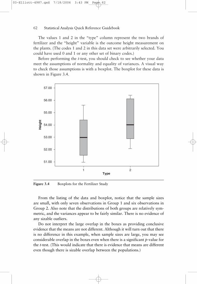
Before performing the t-test, you should check to see whether your datameet the assumptions of normality and equality of variances. A visual wayto check those assumptions is with a boxplot. The boxplot for these data isshown in Figure 3.4.
62——Statistical Analysis Quick Reference Guidebook
57.00
56.00
55.00
54.00
53.00
52.00
51.00
Hei
gh
t
Type1 2
Figure 3.4 Boxplots for the Fertilizer Study
From the listing of the data and boxplot, notice that the sample sizesare small, with only seven observations in Group 1 and six observations inGroup 2. Also note that the distributions of both groups are relatively sym-metric, and the variances appear to be fairly similar. There is no evidence ofany sizable outliers.
Do not interpret the large overlap in the boxes as providing conclusiveevidence that the means are not different. Although it will turn out that thereis no difference in this example, when sample sizes are large, you may seeconsiderable overlap in the boxes even when there is a significant p-value forthe t-test. (This would indicate that there is evidence that means are differenteven though there is sizable overlap between the populations.)
03-Elliott-4987.qxd 7/18/2006 3:43 PM Page 62
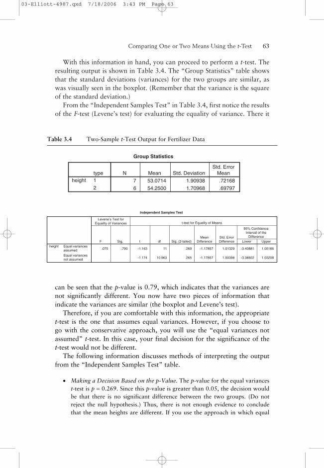
With this information in hand, you can proceed to perform a t-test. Theresulting output is shown in Table 3.4. The “Group Statistics” table showsthat the standard deviations (variances) for the two groups are similar, aswas visually seen in the boxplot. (Remember that the variance is the squareof the standard deviation.)
From the “Independent Samples Test” in Table 3.4, first notice the resultsof the F-test (Levene’s test) for evaluating the equality of variance. There it
Comparing One or Two Means Using the t-Test——63
Table 3.4 Two-Sample t-Test Output for Fertilizer Data
Group Statistics
7 53.0714 1.90938 .72168
6 54.2500 1.70968 .69797
type1
2
heightN Mean Std. Deviation
Std. ErrorMean
Independent Samples Test
.075 .790 -1.163 11 .269 -1.17857 1.01329 -3.40881 1.05166
-1.174 10.963 .265 -1.17857 1.00398 -3.38922 1.03208
Equal variancesassumed
Equal variancesnot assumed
heightF Sig.
Levene’s Test forEquality of Variances
t df Sig. (2-tailed)Mean
DifferenceStd. ErrorDifference Lower Upper
95% ConfidenceInterval of the
Difference
t-test for Equality of Means
can be seen that the p-value is 0.79, which indicates that the variances arenot significantly different. You now have two pieces of information thatindicate the variances are similar (the boxplot and Levene’s test).
Therefore, if you are comfortable with this information, the appropriatet-test is the one that assumes equal variances. However, if you choose togo with the conservative approach, you will use the “equal variances notassumed” t-test. In this case, your final decision for the significance of thet-test would not be different.
The following information discusses methods of interpreting the outputfrom the “Independent Samples Test” table.
• Making a Decision Based on the p-Value. The p-value for the equal variancest-test is p = 0.269. Since this p-value is greater than 0.05, the decision wouldbe that there is no significant difference between the two groups. (Do notreject the null hypothesis.) Thus, there is not enough evidence to concludethat the mean heights are different. If you use the approach in which equal
03-Elliott-4987.qxd 7/18/2006 3:43 PM Page 63

variances are not assumed, the p-value is p = 0.265, which is almost identicalto the “equal variance” p-value. Thus, your decision would be the same.
• Making a Decision Based on the Confidence Interval. The 95% confidenceintervals for the difference in means are given in the last two columns of Table3.4. The interval associated with the assumption of equal variances is (–3.41 to1.05), while the confidence interval when equal variances are not assumed is(–3.39 to 1.03). Since these intervals include 0 (zero), we again conclude thatthere is no significant difference between the means using either assumptionregarding the variances. Thus, you would make the same decisionsdiscussed in the p-value section above. The confidence interval givesmore information than a simple p-value. Each interval above indicates thatplausible values of the mean difference lie between about –3.4 and 1.0.Depending on the nature of your experiment, the information about the rangeof the possible mean differences may be useful in your decision-making process.
Reporting the Results of a (Nonsignificant) Two-Sample t-Test
The following sample write-ups illustrate how you might report this two-sample t-test in publication format. For purposes of illustration, we use the“equal variance” t-test for the remainder of this example:
Narrative for the Methods Section
“A two-sample Student’s t-test assuming equal variances using a pooledestimate of the variance was performed to test the hypothesis that the resultingmean heights of the plants for the two types of fertilizer were equal.”
Narrative for the Results Section
“The mean heights of plants using the two brands of fertilizer were not signif-icantly different, t(11) = –1.17, p = 0.27.”
Or, to be more complete,
“The mean height of plants using fertilizer Brand 1 (M = 53.07, SD = 1.91,N = 7) was not significantly different from that using fertilizer Brand 2(M = 54.25, SD = 1.71, N = 6), t(11) = –1.17, p = 0.27.”
A description of the confidence interval would read as follows:
“A 95% confidence interval on the difference between the two popula-tion means using a Student’s t distribution with 11 degrees of freedom is(–3.41, 1.05), which indicates that there is not significant evidence that thefertilizers produce different mean growth heights.”
64——Statistical Analysis Quick Reference Guidebook
03-Elliott-4987.qxd 7/18/2006 3:43 PM Page 64
SPSS Step-by-Step. EXAMPLE 3.2:Two-Sample t-Test With Equal Variances
To run the two-sample t-test on the FERTILIZER.SAV data, follow thesesteps:
1. Open the data set FERTILIZER.SAV and select Analyze/CompareMeans/Independent Samples T Test. . . .
2. Select Height as the test variable and Type as the grouping variable.
3. Click on the Define Groups button and define the group values as 1 and 2.
4. Click Continue and OK, and the tables shown in Table 3.4 are displayed.
5. To display the boxplot in Figure 3.4, select Graphs/Boxplot and chooseSimple Boxplot and then Define. Select Height as the variable and Type asthe category axis. Click OK.
EXAMPLE 3.3: Two-Sample t-Test With Variance Issues
Describing the Problem
Seventy-six subjects were given an untimed test measuring the dexterityrequired for a particular job skill as a part of a research project at a jobplacement center for inner-city youth. The sample consisted of 17 males and59 females. Time to complete the test was recorded (in minutes). Theresearcher wants to know whether the test is gender neutral. As a part of thatanalysis, she wonders if the average time to complete the test will be thesame for both male and female participants.
Since the researcher is simply interested in determining whether there is adifference in the average times for males and females, a two-sided t-test isappropriate. The hypotheses for this test could be written (in words) as follows:
Null hypothesis (H0): The mean times to finish the skills test are the same forboth genders.
Alternative hypothesis (Ha): The mean times to finish the skills test differ for thetwo genders.
The data for this analysis are entered into a data set in a format similarto the previous example, using one line per subject, with a group variable(gender) containing two values (M and F) and a variable containing the
Comparing One or Two Means Using the t-Test——65
03-Elliott-4987.qxd 7/18/2006 3:43 PM Page 65
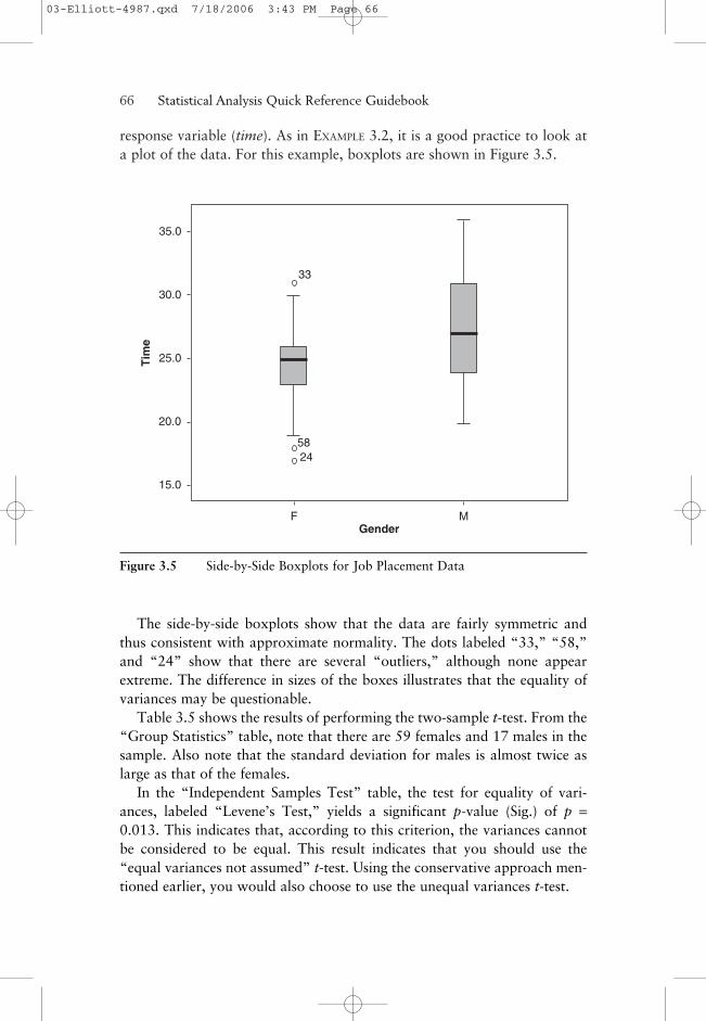
response variable (time). As in EXAMPLE 3.2, it is a good practice to look ata plot of the data. For this example, boxplots are shown in Figure 3.5.
66——Statistical Analysis Quick Reference Guidebook
15.0
20.0
25.0
30.0
35.0
5824
33
Tim
e
F MGender
Figure 3.5 Side-by-Side Boxplots for Job Placement Data
The side-by-side boxplots show that the data are fairly symmetric andthus consistent with approximate normality. The dots labeled “33,” “58,”and “24” show that there are several “outliers,” although none appearextreme. The difference in sizes of the boxes illustrates that the equality ofvariances may be questionable.
Table 3.5 shows the results of performing the two-sample t-test. From the“Group Statistics” table, note that there are 59 females and 17 males in thesample. Also note that the standard deviation for males is almost twice aslarge as that of the females.
In the “Independent Samples Test” table, the test for equality of vari-ances, labeled “Levene’s Test,” yields a significant p-value (Sig.) of p =0.013. This indicates that, according to this criterion, the variances cannotbe considered to be equal. This result indicates that you should use the“equal variances not assumed” t-test. Using the conservative approach men-tioned earlier, you would also choose to use the unequal variances t-test.
03-Elliott-4987.qxd 7/18/2006 3:43 PM Page 66
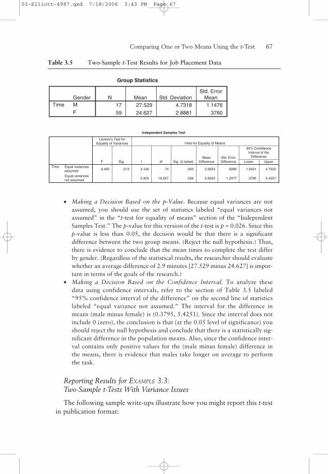
• Making a Decision Based on the p-Value. Because equal variances are notassumed, you should use the set of statistics labeled “equal variances notassumed” in the “t-test for equality of means” section of the “IndependentSamples Test.” The p-value for this version of the t-test is p = 0.026. Since thisp-value is less than 0.05, the decision would be that there is a significantdifference between the two group means. (Reject the null hypothesis.) Thus,there is evidence to conclude that the mean times to complete the test differby gender. (Regardless of the statistical results, the researcher should evaluatewhether an average difference of 2.9 minutes [27.529 minus 24.627] is impor-tant in terms of the goals of the research.)
• Making a Decision Based on the Confidence Interval. To analyze thesedata using confidence intervals, refer to the section of Table 3.5 labeled“95% confidence interval of the difference” on the second line of statisticslabeled “equal variance not assumed.” The interval for the difference inmeans (male minus female) is (0.3795, 5.4251). Since the interval does notinclude 0 (zero), the conclusion is that (at the 0.05 level of significance) youshould reject the null hypothesis and conclude that there is a statistically sig-nificant difference in the population means. Also, since the confidence inter-val contains only positive values for the (male minus female) difference inthe means, there is evidence that males take longer on average to performthe task.
Reporting Results for EXAMPLE 3.3:Two-Sample t-Tests With Variance Issues
The following sample write-ups illustrate how you might report this t-testin publication format:
Comparing One or Two Means Using the t-Test——67
Table 3.5 Two-Sample t-Test Results for Job Placement Data
Group Statistics
17 27.529 4.7318 1.1476
59 24.627 2.8881 .3760
GenderM
F
TimeN Mean Std. Deviation
Std. ErrorMean
Independent Samples Test
6.450 .013 3.126 74 .003 2.9023 .9285 1.0521 4.7525
2.403 19.557 .026 2.9023 1.2077 .3795 5.4251
Equal variancesassumed
Equal variancesnot assumed
Time
F Sig.
Levene’s Test forEquality of Variances
t df Sig. (2-tailed)Mean
DifferenceStd. ErrorDifference Lower Upper
95% ConfidenceInterval of the
Difference
t-test for Equality of Means
03-Elliott-4987.qxd 7/18/2006 3:43 PM Page 67
Narrative for the Methods Section
“Since a preliminary Levene’s test for equality of variances indicated that thevariances of the two groups were significantly different, a two-sample t-testwas performed that does not assume equal variances.”
Narrative for the Results Section
“There is evidence within the setting observed that males take a significantlylonger time on average to complete the untimed skills test than do females,t(19.6) = 2.40, p = 0.03.”
Or, more completely,
“The mean time required for females to complete the untimed aptitude test(M = 24.6 minutes, SD = 2.89, N = 59) was significantly shorter than that requiredfor males (M = 27.53 minutes, SD = 4.73, N = 17), t(20) = 2.40, p = 0.03.”
SPSS Step-by-Step. EXAMPLE 3.3:Two-Sample t-Tests With Variance Issues
To create the side-by-side boxplots, use the following steps:
1. Open the data set JOB.SAV and select Graph/Boxplot/Simple . . . and clickDefine.
2. Select Time as the variable and Gender for the category axis.
3. Click OK, and the plot shown in Figure 3.5 will be displayed.
To create the t-test output in SPSS for this example, follow these steps:
1. Using the data set JOB.SAV, select Analyze/Compare Means/IndependentSamples T Test. . . .
2. Select Time as the test variable and Gender as the grouping variable.
3. Click on the Define Groups button and define the group values as M and F.
4. Click Continue and then OK, and the output shown in Table 3.5 appears.
Paired t-Test
The paired t-test is appropriate for data in which the two samples are pairedin some way. This type of analysis is appropriate for three separate datacollection scenarios:
68——Statistical Analysis Quick Reference Guidebook
03-Elliott-4987.qxd 7/18/2006 3:43 PM Page 68
• Pairs consist of before and after measurements on a single group of subjectsor patients.
• Two measurements on the same subject or entity (right and left eye, forexample) are paired.
• Subjects in one group (e.g., those receiving a treatment) are paired or matchedon a one-to-one basis with subjects in a second group (e.g., control subjects).
In all cases, the data to be analyzed are the differences within pairs (e.g.,the right eye measurement minus the left eye measurement). The differencescores are then analyzed as a one-sample t-test.
Associated Confidence Interval
The confidence interval associated with a paired t-test is the same asthe confidence interval for a one-sample t-test using the difference scores.The resulting confidence interval is usually examined to determine whetherit includes zero.
Appropriate Applications for a Paired t-Test
The following are examples of paired data that would properly be ana-lyzed using a paired t-test.
• Does the Diet Work? A developer of a new diet is interested in showing thatit is effective. He randomly chooses 15 subjects to go on the diet for 1 month.He weighs each patient before and after the 1-month period to see whetherthere is evidence of a weight loss at the end of the month.
• Is a New Teaching Method Better Than Standard Methods? An educatorwants to test a new method for improving reading comprehension. Twentystudents are assigned to a section that will use the new method. Each of these20 students is matched with a student with similar reading ability who willspend the semester in a class using the standard teaching methods. At the endof the semester, the students in both sections will be given a common readingcomprehension exam, and the average reading comprehension of the twogroups is compared.
• Does a New Type of Eye Drops Work Better Than Standard Drops? A phar-maceutical company wants to test a new formulation of eye drops with itsstandard drops for reducing redness. Fifty subjects who have similar problemswith eye redness in each eye are randomly selected for the study. For eachsubject, an eye is randomly selected to be treated with the new drops, and theother eye is treated with the standard drops. At the end of the treatmentschedule, the redness in each eye is measured using a quantitative scale.
Comparing One or Two Means Using the t-Test——69
03-Elliott-4987.qxd 7/18/2006 3:43 PM Page 69
Design Considerations for a Paired t-Test
Pairing Observations May Increase the Ability to Detect Differences
A paired t-test is appropriate when variability between groups may besufficiently large to mask any mean differences that might exist betweenthe groups. Pairing is a method of obtaining a more direct measurement onthe difference being examined. For example, in the diet example above, onemethod of assessing the performance of the diet would be to select 30 sub-jects and randomly assign 15 to go on the diet and 15 to eat regularly for thenext month (i.e., the control group). At the end of the month, the weights ofthe subjects on the diet could be compared with those in the control groupto determine whether there is evidence of a difference in average weights.Clearly, this is not a desirable design since the variability of weights ofsubjects within the two groups will likely mask any differences that mightbe produced by one month on the diet. A better design would be to select 15subjects and measure the weights of these subjects before and after themonth on the diet. The 15 differences between the before and after weightsfor the subjects provide much more focused measurements of the effect ofthe diet than would independent samples.
Paired t-Test Analysis Is Performed on the Difference Scores
The data to be analyzed in a paired t-test are the differences between pairs(e.g., the before minus after weight for each subject in a diet study or differ-ences between matched pairs in the study of teaching methods). The differ-ence scores are then analyzed using a one-sample t-test.
The Paired t-Test Assumes Normality of the Differences
The basic assumption for the paired t-test to be valid when you havesmall sample sizes is that the difference scores are normally distributed andthat the observed differences represent a random sample from the popula-tion of differences. (See the section on testing for normality, “DescribingQuantitative Data,” in Chapter 2.)
Hypotheses for a Paired t-Test
The hypotheses to be tested in a paired t-test are similar to those used ina two-sample t-test. In the case of paired data, µ1 and µ 2 refer to the popu-lation means of the before and after measurements on a single group of sub-jects or to the first and second pair in the case of matched subjects. The null
70——Statistical Analysis Quick Reference Guidebook
03-Elliott-4987.qxd 7/18/2006 3:43 PM Page 70
hypotheses may be stated as H0: µ1 = µ2. However, in the case of paired data,it is common practice to make use of the fact that the difference between thetwo population means (i.e., µ1 – µ2) is equal to the population mean of thedifference scores, denoted µd. In this case, the hypotheses are written asfollows:
H0: µd = 0 (the population mean of the differences is zero).
Ha: µd ≠ 0 (the population mean of the differences is not zero).
EXAMPLE 3.4: Paired t-Test
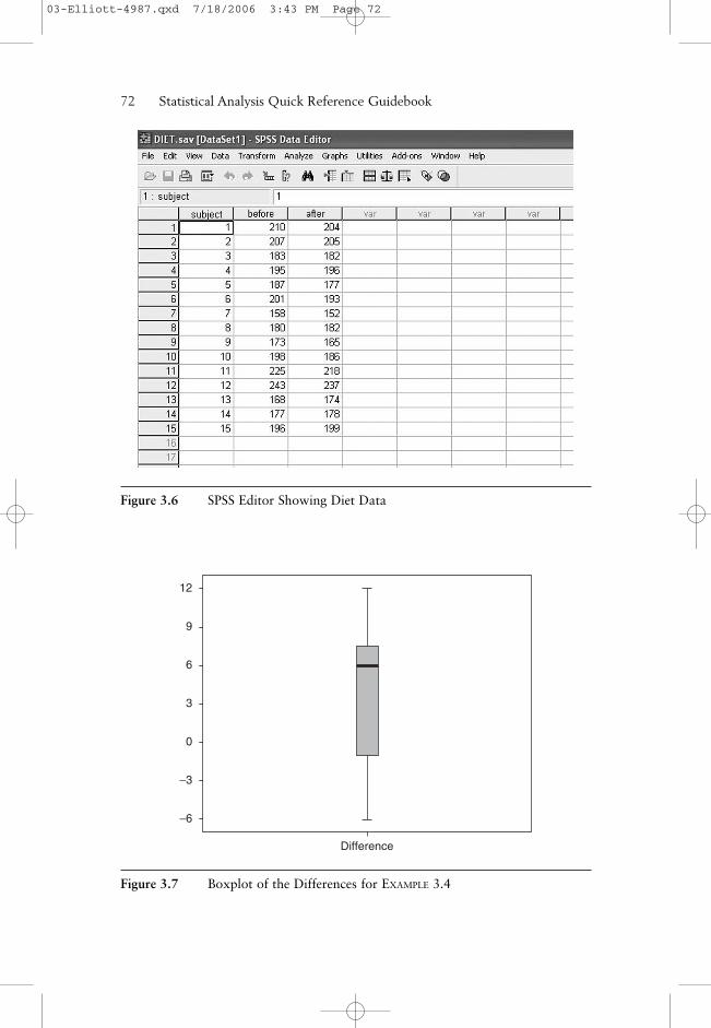
Consider the diet example described above. The data for this exampleinclude two variables reporting before and after weights for 15 randomlyselected subjects who participated in a test of a new diet for a 1-monthperiod. Figure 3.6 illustrates the data format, where it can be seen that thebefore and after weights for a subject are entered on the same row. In thiscase, we want to determine whether there is evidence that the diet works.That is, if we calculate differences as di = “before” weight minus “after”weight, then we should test the following hypotheses:
H0 : µd = 0 (the mean of the differences is zero; i.e., the diet is ineffective).
Ha : µd > 0 (the mean of the differences is positive; i.e., the diet is effective).
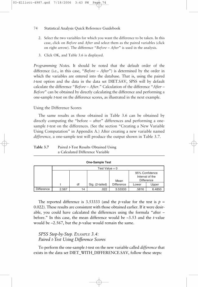
The first step in the analysis is to simply observe the distribution of thedifferences using a boxplot. Figure 3.7 shows the plot for the diet data.
This plot shows that the distribution of the differences is fairly symmetricand that the assumption of normality seems reasonable. Also, it can be seenthat only a small percentage of the differences were below 0 (no weight lossor negative weight loss).
To analyze the data using a statistical test, we examine the output in the“Paired Samples Test” shown in Table 3.6.
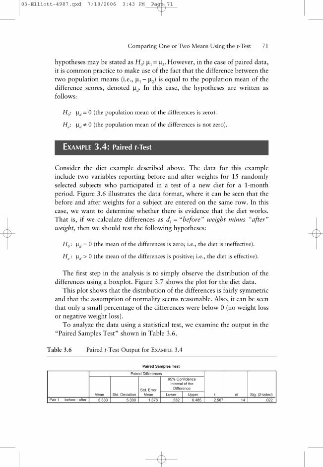
Comparing One or Two Means Using the t-Test——71
Paired Samples Test
3.533 5.330 1.376 .582 6.485 2.567 14 .022before - afterPair 1Mean Std. Deviation
Std. ErrorMean Lower Upper
95% ConfidenceInterval of the
Difference
Paired Differences
t df Sig. (2-tailed)
Table 3.6 Paired t-Test Output for EXAMPLE 3.4
03-Elliott-4987.qxd 7/18/2006 3:43 PM Page 71
72——Statistical Analysis Quick Reference Guidebook
Figure 3.6 SPSS Editor Showing Diet Data
12
9
6
3
0
−3
−6
Difference
Figure 3.7 Boxplot of the Differences for EXAMPLE 3.4
03-Elliott-4987.qxd 7/18/2006 3:43 PM Page 72

In this output, it can be seen that the sample mean of the difference scoresis 3.533, with a standard deviation of the differences given by 5.330. Thecalculated t-statistic (with 14 df) is given by 2.567, which has a p-value of0.022. When interpreting these results, you should notice that the mean ofthe “before minus after” differences is positive, which is supportive of thealternative hypothesis that µd > 0. Since this experiment from its inceptionwas only interested in detecting a weight loss, it can be viewed as a one-sidedtest. Thus, for a one-sided hypothesis test, the reported p-value should beone-half of the p-value given in the computer output (i.e., p = 0.011). Thatis, at the α = .05 level, we reject H0 and conclude that the diet is effective.The output also includes a 95% confidence interval on the mean difference.It should be noted that this confidence interval is a two-sided confidenceinterval. In this case, the fact that the confidence interval (0.58, 6.49) con-tains only positive values suggests that µd > 0 (i.e., that the diet is effective).
Reporting the Results for EXAMPLE 3.4: Paired t-Test
The following sample write-ups illustrate how you might report thispaired t-test in publication format.
Narrative for the Methods Section
“A paired t-test was performed to ascertain whether the diet was effective.”
Narrative for the Results Section
“There is evidence that the mean weight loss is positive, that is, that the diet iseffective in producing weight loss, t(14) = 2.567, one-tailed p = 0.01.”
Or, more completely,
“The mean weight loss (M = 3.53, SD = 5.33, N = 15) was significantly greaterthan zero, t(14) = 2.567, one-tailed p = 0.01, providing evidence that the dietis effective in producing weight loss.”
SPSS Step-by Step. EXAMPLE 3.4: Paired t-Test
It should be noted that SPSS can be used to perform a paired t-test in twodifferent ways.
Using the Data Pairs
1. Open the data set DIET.SAV and select Analyze/Compare Means/Paired-Samples T Test. . . .
Comparing One or Two Means Using the t-Test——73
03-Elliott-4987.qxd 7/18/2006 3:43 PM Page 73
2. Select the two variables for which you want the difference to be taken. In thiscase, click on Before and After and select them as the paired variables (clickon right arrow). The difference “Before – After” is used in the analysis.
3. Click OK, and Table 3.6 is displayed.
Programming Notes. It should be noted that the default order of thedifference (i.e., in this case, “Before – After”) is determined by the order inwhich the variables are entered into the database. That is, using the pairedt-test option and the data in the data set DIET.SAV, SPSS will by defaultcalculate the difference “Before – After.” Calculation of the difference “After –Before” can be obtained by directly calculating the difference and performing aone-sample t-test on the difference scores, as illustrated in the next example.
Using the Difference Scores
The same results as those obtained in Table 3.6 can be obtained bydirectly computing the “before – after” differences and performing a one-sample t-test on the differences. (See the section “Creating a New VariableUsing Computation” in Appendix A.) After creating a new variable nameddifference, a one-sample test will produce the output shown in Table 3.7.
74——Statistical Analysis Quick Reference Guidebook
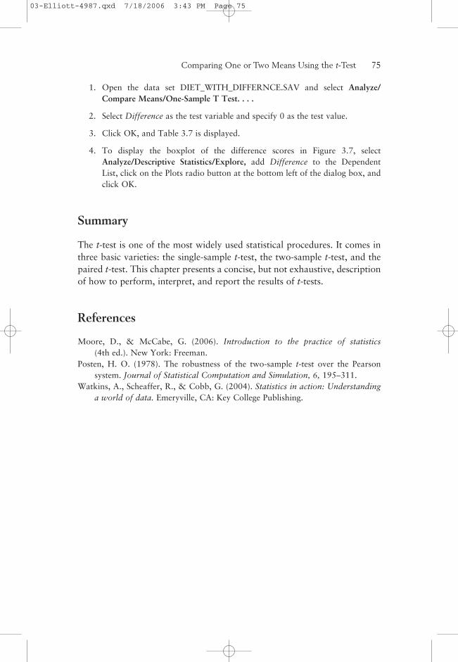
Table 3.7 Paired t-Test Results Obtained Usinga Calculated Difference Variable
One-Sample Test
2.567 14 .022 3.53333 .5816 6.4850Difference
t df Sig. (2-tailed)Mean
Difference Lower Upper
95% ConfidenceInterval of the
Difference
Test Value = 0
The reported difference is 3.53333 (and the p-value for the test is p =0.022). These results are consistent with those obtained earlier. If it were desir-able, you could have calculated the differences using the formula “after –before.” In this case, the mean difference would be –3.53 and the t-valuewould be –2.567, but the p-value would remain the same.
SPSS Step-by-Step. EXAMPLE 3.4:Paired t-Test Using Difference Scores
To perform the one-sample t-test on the new variable called difference thatexists in the data set DIET_WITH_DIFFERENCE.SAV, follow these steps:
03-Elliott-4987.qxd 7/18/2006 3:43 PM Page 74
1. Open the data set DIET_WITH_DIFFERNCE.SAV and select Analyze/Compare Means/One-Sample T Test. . . .
2. Select Difference as the test variable and specify 0 as the test value.
3. Click OK, and Table 3.7 is displayed.
4. To display the boxplot of the difference scores in Figure 3.7, selectAnalyze/Descriptive Statistics/Explore, add Difference to the DependentList, click on the Plots radio button at the bottom left of the dialog box, andclick OK.
Summary
The t-test is one of the most widely used statistical procedures. It comes inthree basic varieties: the single-sample t-test, the two-sample t-test, and thepaired t-test. This chapter presents a concise, but not exhaustive, descriptionof how to perform, interpret, and report the results of t-tests.
References
Moore, D., & McCabe, G. (2006). Introduction to the practice of statistics(4th ed.). New York: Freeman.
Posten, H. O. (1978). The robustness of the two-sample t-test over the Pearsonsystem. Journal of Statistical Computation and Simulation, 6, 195–311.
Watkins, A., Scheaffer, R., & Cobb, G. (2004). Statistics in action: Understandinga world of data. Emeryville, CA: Key College Publishing.
Comparing One or Two Means Using the t-Test——75
03-Elliott-4987.qxd 7/18/2006 3:43 PM Page 75
03-Elliott-4987.qxd 7/18/2006 3:43 PM Page 76