Comparing neuro-dynamic programming algorithms for...

*Current a$liation and address: PROS Strategic Solutions, 3223 Smith Street, Suite 100, Houston, TX, 77006, USA.Tel.: #1-713-335-5840; fax: #1-713-523-8144.

E-mail address: [email protected] (N. Secomandi)

Computers & Operations Research 27 (2000) 1201}1225

Comparing neuro-dynamic programming algorithms for thevehicle routing problem with stochastic demands

Nicola Secomandi*

Department of Decision and Information Sciences, College of Business Administration, University of Houston, Houston,TX 77204-6282, USA

Abstract

The paper considers a version of the vehicle routing problem where customers' demands are uncertain. Thefocus is on dynamically routing a single vehicle to serve the demands of a known set of geographicallydispersed customers during real-time operations. The goal consists of minimizing the expected distancetraveled in order to serve all customers' demands. Since actual demand is revealed upon arrival of the vehicleat the location of each customer, fully exploiting this feature requires a dynamic approach.

This work studies the suitability of the emerging "eld of neuro-dynamic programming (NDP) in providingapproximate solutions to this di$cult stochastic combinatorial optimization problem. The paper comparesthe performance of two NDP algorithms: optimistic approximate policy iteration and a rollout policy. Whilethe former improves the performance of a nearest-neighbor policy by 2.3%, the computational resultsindicate that the rollout policy generates higher quality solutions. The implication for the practitioner is thatthe rollout policy is a promising candidate for vehicle routing applications where a dynamic approach isrequired.

Scope and purpose

Recent years have seen a growing interest in the development of vehicle routing algorithms to cope withthe uncertain and dynamic situations found in real-world applications (see the recent survey paper by Powellet al. [1]). As noted by Psaraftis [2], dramatic advances in information and communication technologiesprovide new possibilities and opportunities for vehicle routing research and applications. The enhancedcapability of capturing the information that becomes available during real-time operations opens upnew research directions. This informational availability provides the possibility of developing dynamicrouting algorithms that take advantage of the information that is dynamically revealed during operations.Exploiting such information presents a signi"cant challenge to the operations research/management sciencecommunity.

0305-0548/00/$ - see front matter ( 2000 Elsevier Science Ltd. All rights reserved.PII: S 0 3 0 5 - 0 5 4 8 ( 9 9 ) 0 0 1 4 6 - X

The single vehicle routing problem with stochastic demands [3] provides an example of a simple, yet verydi$cult to solve exactly, dynamic vehicle routing problem [2, p. 157]. The problem can be formulated asa stochastic shortest path problem [4] characterized by an enormous number of states.

Neuro-dynamic programming [5,6] is a recent methodology that can be used to approximately solve verylarge and complex stochastic decision and control problems. In this spirit, this paper is meant to study theapplicability of neuro-dynamic programming algorithms to the single-vehicle routing problem with stochas-tic demands. ( 2000 Elsevier Science Ltd. All rights reserved.

Keywords: Stochastic vehicle routing; Neuro-dynamic programming; Rollout policies; Heuristics

1. Introduction

The deterministic vehicle routing problem (VRP) is well studied in the operations researchliterature (see [3,7}10] for reviews). Given a set of geographically dispersed customers, eachshowing a positive demand for a given commodity, VRP consists of "nding a set of tours ofminimum length for a #eet of vehicles located at a central depot, such that customers' demands aresatis"ed and vehicles' capacities are not exceeded.

This work deals with a variation where customers' demands are uncertain and are assumed tofollow given discrete probability distributions. This situation arises in practice whenever a distribu-tion company faces the problem of deliveries to a set of customers, whose demands are uncertain.This work focuses on deliveries, but all the discussion carries through in case of collections. Theproblem of "nding a tour through the customers that minimizes expected distance traveled isknown as the vehicle routing problem with stochastic demands (SVRP for short) [11}14]. Otherauthors have considered the additional case where the presence of customers is also uncertain (i.e.,customers are present with a known probability). This variation is known as the vehicle routingproblem with stochastic customers and demands [12,14}16]. This paper only considers the case ofstochastic demands.

Stochastic vehicle routing problems may be employed to model a number of business situationsthat arise in the area of distribution. Some examples follow (note that some of the references do notnecessarily indicate a stochastic or dynamic formulation). In a strategic planning scenario, afterhaving identi"ed some major customers a distribution company might be interested in estimatingthe expected amount of travel to serve these customers on a typical day [12]. Central banks face theproblem of delivering money to branches or automatic teller machines whose requirements vary ona daily basis [17]. In less-than-truckload operations the amount of goods to be collected on anygiven day from a set of customers is generally uncertain [15]. Other examples of applicationsreported in the literature include the delivery of home heating oil [18], sludge disposal [19], thedesign of a `hot mealsa delivery system [20], and routing of forklifts in a cargo terminal or ina warehouse [12]. Psaraftis [2] provides examples of more `dynamica situations, where the timedimension is an essential feature of the problem: courier services, intermodal services, tram shipoperations, combined pickup and delivery services, and management of container terminals.

Most works in the literature [14] dealing with versions of the stochastic VRP focus oncomputing a "xed order of customers' visitation, eventually supplemented by decision rules on

1202 N. Secomandi / Computers & Operations Research 27 (2000) 1201}1225

when to return to the depot to replenish, in anticipation of route failures. A route failure occurswhen, due to the variability associated with customers' demands, the vehicle capacity is exceeded.Recourse actions are taken when a route failure occurs. A popular recourse action employed in theliterature consists of having the vehicle return to the depot, replenish and resume its tour from thelocation where the failure occurred.

More speci"cally, properties and formulations of the problem are investigated by Dror et al.[11], Dror [21], and Bastian and Rinnooy Kan [22]. Bertsimas [12] proposes an asymptoticallyoptimal heuristic, and an expression to e$ciently compute the expected length of a tour. Bertsimaset al. [13] investigate the empirical behavior of this heuristic, and enhance it by using dynamicprogramming (DP) to supplement the a priori tour with rules for selecting return trips to the depot.Yang et al. [23] extend this approach to the multi-vehicle case when the length of each tour cannotexceed a given threshold. Secomandi [24] develops rollout algorithms to improve on any initialtour. A simulated annealing heuristic is proposed by TeodorovicH and PavkovicH [25]. Otherheuristics are developed by Dror and Trudeau [26], Dror et al. [27], and BouzamK ene-Ayari et al.[28]. Gendreau et al. [15] propose an exact algorithm based on the integer L-shaped method ofLaporte and Louveaux [29] for the case of both stochastic customers and demands. They alsoderive a DP-based algorithm to compute the expected length of a tour. The same authors [16]develop a tabu search heuristic to be used in case of large size instances. The chance constrainedversion of the problem is considered by Golden and Yee [30], Stewart and Golden [31], andLaporte et al. [32].

These approaches, with the partial exception of Bertsimas et al. [13], Yang et al. [23], andSecomandi [24] treat the problem as static, whereby the order of customers' visitation is notchanged during its real-time execution when the actual demands' realizations become available.

The recent survey by Psaraftis [2] emphasizes the e!ect on the "eld of vehicle routing ofdramatic advances in computer-based technology, such as electronic data interchange, geographicinformation systems, global positioning systems, and intelligent vehicle-highway systems. Hestresses the concept that the enhanced availability of real-time data allowed by these technologiesopens new challenges and research directions for the operations research/management sciencecommunity. In particular, such technologies provide the necessary informational support fordeveloping dynamic vehicle routing algorithms that can exploit the wealth of information thatbecomes available during real-time operations. The work of Powell et al. [1] provides an excellentreview of dynamic and stochastic routing problems from an operations research/managementscience perspective.

In this context, Psaraftis presents the work of Dror et al. [11] as the "rst dynamic formulation ofSVRP. He considers this model as a simple, yet di$cult to solve exactly, dynamic routing problem.These authors develop a large-scale Markov decision process (MDP) model for SVRP, but nocomputational experience is provided. A slightly modi"ed version of this model is discussed byDror [21]. No computational experience is performed, and the author considers instances withmore than three customers as computationally intractable (a comment also made by Dror et al.[27]). Secomandi [24] reformulates the problem as a stochastic shortest path problem (SSPP) andby exploiting a state-space decomposition develops an exact DP algorithm that can solve smallinstances (about 10 customers) to optimality. He also derives properties of the optimal policy.

Neuro-dynamic programming, also known as reinforcement learning (NDP for short), is a recentmethodology that deals with the approximate solution of large and complex DP problems. (See the

N. Secomandi / Computers & Operations Research 27 (2000) 1201}1225 1203

recent books by Bertsekas and Tsitsiklis [5] and by Sutton and Barto [6] for excellent presenta-tions of NDP.) NDP combines simulation, learning, approximation architectures (e.g., neuralnetworks) and the central ideas of DP to break the curse of dimensionality typical of DP.

In this spirit, the goal of this work is to study the applicability of the NDP methodology to theSSPP formulation of the single-vehicle SVRP in order to compute a suboptimal dynamic routingpolicy. The large-scale SSPP formulation analyzed in Secomandi [24] is adopted. The papercompares two NDP algorithms based on the approximate policy iteration (API) scheme: optimisticAPI and a rollout policy (RP). (The reader is referred to Secomandi [24] for a discussion of thetheoretical properties of RP when applied to SVRP.)

Although a simpli"ed model of a potential real-world distribution application, the single-vehicleSVRP does present some features that characterize it as an interesting dynamic routing problem. Ina real-world application a distribution manager is likely to operate a #eet of vehicles. In this workthe following assumption holds throughout: a set of customers has been assigned to be served bya given vehicle. Therefore, the multi-vehicle problem decomposes into independent single-vehiclesubproblems. A scheme of this type has been proposed in the context of a stochastic and dynamicrouting problem discussed by Bertsimas and van Ryzin [33}35]. In their work, requests for servicearriving over time are assigned to the log of individual vehicles, e!ectively reducing the routing partof the problem to a situation somewhat similar to that studied here.

The paper is organized as follows. Section 2 introduces the problem. Section 3 presents aSSPP formulation for SVRP. Section 4 discusses the NDP approach. The NDP methodology isapplied to SVRP in Section 5. Experimental analysis of the algorithms is conducted in Section 6.Section 7 concludes the paper.

2. Problem description

2.1. Notation and assumptions

Let the set of nodes of a given complete network be M0, 1,2, nN. Node 0 denotes the depotand <"M1, 2,2, nN represents the set of customers' locations. Distances d(i, j) betweennodes are assumed to be known and symmetric, and they satisfy the triangle inequality:d(i, j))d(i, k)#d(k, j). Q denotes vehicle capacity. A single vehicle is assumed. This is equivalentto assuming that a set of customers has been assigned to receive service by a given vehicle. LetD

i, i"1, 2,2, n, be the random variable that describes the demand of customer i. The probability

distribution of Diis discrete and known, and is denoted by p

i(k),PrMD

i"kN, k"0, 1,2, K)Q.

Customers' demands are assumed to be stochastically independent, and their realizations becomeknown upon the "rst arrival of the vehicle at each customer location. The vehicle is initially locatedat the depot. During service, when capacity is reached or exceeded, a return trip to the depot isperformed in order to restore capacity up to Q. This implies that the depot capacity is assumed tobe at least equal to nK. When all demands have been satis"ed, the vehicle returns to the depot. Theobjective is to determine a service/routing policy such that demand at each node is met, andexpected distance traveled is minimized.

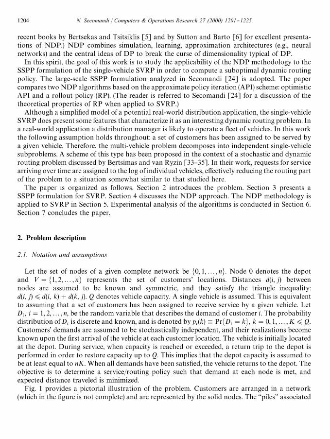
Fig. 1 provides a pictorial illustration of the problem. Customers are arranged in a network(which in the "gure is not complete) and are represented by the solid nodes. The `pilesa associated


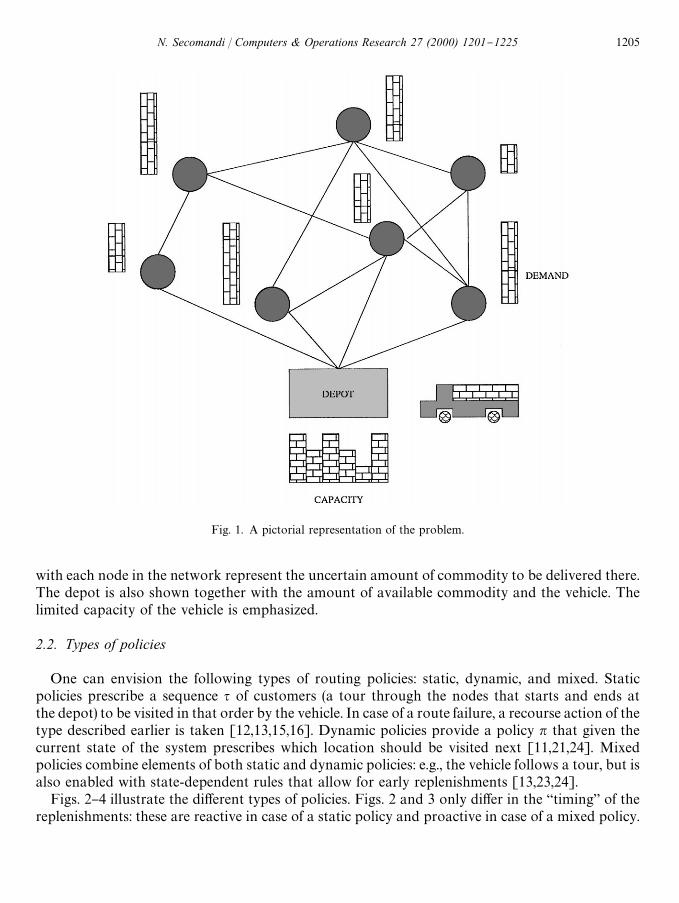
Fig. 1. A pictorial representation of the problem.

with each node in the network represent the uncertain amount of commodity to be delivered there.The depot is also shown together with the amount of available commodity and the vehicle. Thelimited capacity of the vehicle is emphasized.

2.2. Types of policies

One can envision the following types of routing policies: static, dynamic, and mixed. Staticpolicies prescribe a sequence q of customers (a tour through the nodes that starts and ends atthe depot) to be visited in that order by the vehicle. In case of a route failure, a recourse action of thetype described earlier is taken [12,13,15,16]. Dynamic policies provide a policy n that given thecurrent state of the system prescribes which location should be visited next [11,21,24]. Mixedpolicies combine elements of both static and dynamic policies: e.g., the vehicle follows a tour, but isalso enabled with state-dependent rules that allow for early replenishments [13,23,24].

Figs. 2}4 illustrate the di!erent types of policies. Figs. 2 and 3 only di!er in the `timinga of thereplenishments: these are reactive in case of a static policy and proactive in case of a mixed policy.


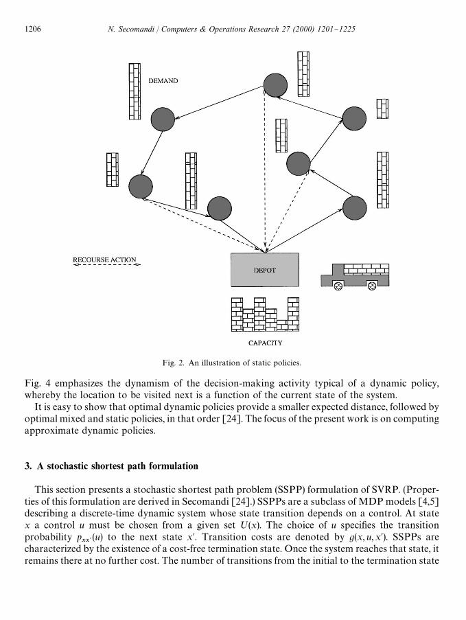
Fig. 2. An illustration of static policies.

Fig. 4 emphasizes the dynamism of the decision-making activity typical of a dynamic policy,whereby the location to be visited next is a function of the current state of the system.

It is easy to show that optimal dynamic policies provide a smaller expected distance, followed byoptimal mixed and static policies, in that order [24]. The focus of the present work is on computingapproximate dynamic policies.

3. A stochastic shortest path formulation

This section presents a stochastic shortest path problem (SSPP) formulation of SVRP. (Proper-ties of this formulation are derived in Secomandi [24].) SSPPs are a subclass of MDP models [4,5]describing a discrete-time dynamic system whose state transition depends on a control. At statex a control u must be chosen from a given set ;(x). The choice of u speci"es the transitionprobability p

xx{(u) to the next state x@. Transition costs are denoted by g(x, u,x@). SSPPs are

characterized by the existence of a cost-free termination state. Once the system reaches that state, itremains there at no further cost. The number of transitions from the initial to the termination state


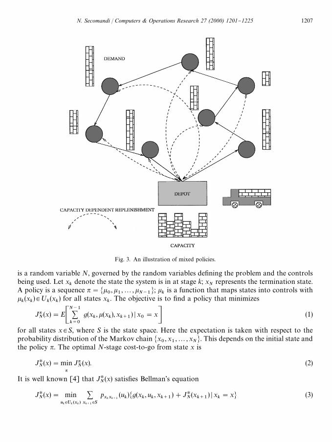
Fig. 3. An illustration of mixed policies.

is a random variable N, governed by the random variables de"ning the problem and the controlsbeing used. Let x

kdenote the state the system is in at stage k; x

Nrepresents the termination state.

A policy is a sequence n"Mk0, k

1,2,k

N~1N; k

kis a function that maps states into controls with

kk(x

k)3;

k(x

k) for all states x

k. The objective is to "nd a policy that minimizes

JnN(x)"EC

N~1+k/0

g(xk, k(x

k), x

k`1) D x

0"xD (1)

for all states x3S, where S is the state space. Here the expectation is taken with respect to theprobability distribution of the Markov chain Mx

0, x

1,2, x

NN. This depends on the initial state and

the policy n. The optimal N-stage cost-to-go from state x is

JHN(x)"min

nJnN(x). (2)

It is well known [4] that JHN(x) satis"es Bellman's equation

JHN(x)" min

uk|Uk (xk )

+xk`1|S

pxkxk`1

(uk)Mg(x

k, u

k, x

k`1)#JH

N(x

k`1) D x

k"xN (3)


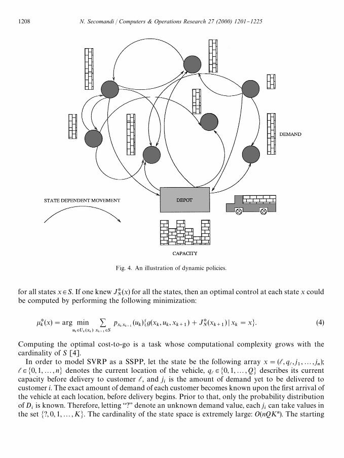
Fig. 4. An illustration of dynamic policies.

for all states x3S. If one knew JHN(x) for all the states, then an optimal control at each state x could

be computed by performing the following minimization:

kHk(x)"arg min

uk|Uk (xk )

+xk`1|S

pxkxk`1

(uk)Mg(x

k, u

k, x

k`1)#JH

N(x

k`1) D x

k"xN. (4)

Computing the optimal cost-to-go is a task whose computational complexity grows with thecardinality of S [4].

In order to model SVRP as a SSPP, let the state be the following array x"(l, ql , j1,2, j

n);

l3M0, 1,2, nN denotes the current location of the vehicle, ql3M0, 1,2, QN describes its currentcapacity before delivery to customer l, and j

iis the amount of demand yet to be delivered to

customer i. The exact amount of demand of each customer becomes known upon the "rst arrival ofthe vehicle at each location, before delivery begins. Prior to that, only the probability distributionof D

iis known. Therefore, letting `?a denote an unknown demand value, each j

ican take values in

the set M?, 0, 1,2, KN. The cardinality of the state space is extremely large: O(nQKn). The starting


state is (0,Q, ?, ?,2, ?), the "nal (0,Q, 0, 0,2, 0). At a given state x, the control set is;(x)"MMm3M1, 2,2, nN D j

mO0NXM0NN]Ma: a3M0, 1NN; i.e., any not yet visited customer m, or one

with a pending demand, directly from l (a"0), or by "rst visiting the depot (a"1); the depot isalso included when all demands are satis"ed, so that the vehicle moves there and the system entersthe termination state. Alternative a"1 allows some #exibility, whereby preventive trips to thedepot are executed in order to avoid future expensive route failures. The control set of a given stateis constrained such that at a customer location the demand is satis"ed to the maximum extent,given the current capacity. Therefore, a control u assumes the form of a pair (m, a). (When alldemands are satis"ed u,(0, 0).) From state x"(l,ql , j

1,2, j

m,2, j

n) the system moves to state

x@"(m, qm, j

1,2, j@

m,2, j

n). The transition cost from state x to state x@ under control u is

g(x, u,x@)"Gd(l,m) if u"(m, 0),

d(l, 0)#d(0,m) if u"(m, 1).

The capacity at x@ is updated to be

qm"G

max(0, ql!jl) if u"(m, 0),

ql#Q!jl if u"(m, 1).

If jm"? at x, j@

mis de"ned to be a realization of the random variable D

m, otherwise j@

m"j

m.

Transition probabilities are simply

pxx{

"G1 if j

mis known,

PrMDm"j@

mN otherwise.

This formulation is exploited in Section 5 to develop NDP algorithms for computing a suboptimalpolicy for SVRP. The key point here is that JH

N(x) is not known and its computation is an

intractable task. Therefore, computationally tractable ways to approximate such function aresought. The next section discusses this issue from the NDP standpoint.

4. Neuro-dynamic programming

NDP is a methodology designed to deal with large or complex DP problems (see the work ofBertsekas and Tsitsiklis [5] and that of Sutton and Barto [6] for excellent introductions to theNDP "eld). With such problems, the large state space or the lack of an explicit model of the systemprevent the applicability of the exact methods of DP [4]. In the present setting, a model of thesystem is available, but the size of its state space is large. Therefore computing the optimalcost-to-go is computationally prohibitive. To motivate NDP, observe that an approximate policycan still be implemented if the optimal cost-to-go JH( ) ) is replaced by an approximation JI ( ) ). (Inthe remainder of the paper the subscript N on the cost-to-go is dropped for notational conveni-ence.) This is accomplished by computing approximate controls k8

k( ) ) as follows:

k8k(x)"arg min

uk|Uk (xk )

+xk`1|S

pxkxk`1

(uk)Mg(x

k, u

k, x

k`1)#JI (x

k`1) D x

k"xN. (5)


Note that (5) is essentially an approximation of minimization (4) with JH( ) ) replaced by JI ( ) ). This isthe idea at the heart of NDP. The methodology consists of a rich set of algorithms to compute theapproximation JI ( ) ). In the following a few possibilities are considered.

The model-free case where an explicit model of the system is not available (e.g., the transitionprobabilities are not available in closed form) can also be dealt with by NDP, but is not discussedhere. The reader is referred to the recent monographs by Bertsekas and Tsitsiklis [5] and by Suttonand Barto [6].

4.1. Approximate policy iteration

The main idea of NDP is to break the barriers posed by a large state space or the lack of anexplicit model of the system by employing simulation and parametric function approximations.Approximate policy iteration (API) is a NDP algorithm that focuses on the approximate executionof the policy iteration algorithm (see [4,5, pp. 269}284]). The exact policy iteration algorithm isdescribed below. Assume that an initial policy k1 is available.(1) Perform a policy evaluation step to compute Jk1(x), for all states x3S, by solving the system of

linear equations

Jk1(x)" +xk`1|S

pxkxk`1

(k1k(x

k))Mg(x

k, k1

k(x

k),x

k`1)#Jk1(x

k`1) D x

k"xN, ∀x3S. (6)

(2) Perform a policy improvement step which computes a new policy k2 as follows:

k2k(x)"arg min

uk|Uk (xk )

+xk`1|S

pxkxk`1

(uk)Mg(x

k, u

k, x

k`1)#Jk1(x

k`1) D x

k"xN, ∀x3S. (7)

These steps are repeated until Jkm"Jkm`1, ∀x3S, in which case the algorithm can be shown to

terminate with the optimal policy km [4].It is clear that when dealing with large-scale systems this algorithm is not a viable avenue. But its

steps can be approximated. NDP replaces the cost-to-go Jk(x) of a policy k by an approximationJI k(x, r) that depends on a vector of parameters r. This approximation could be linear or nonlinear(e.g., a neural network). This process is now outlined [5].(1) Approximate policy evaluation.

f Assume that under the current policy k pairs of states and sample cost-to-go valuesbelonging to k have been collected by simulation. In the neural network terminology, thisconsists in the generation of a `training seta for the policy k. If an initial policy is notavailable, one can always be obtained by arbitrarily "xing the vector of parameters r, andtaking approximately greedy controls with respect to the cost-to-go de"ned by r using (5).

f Perform a least-squares "tting (linear or nonlinear, depending on the type of functionapproximation being used) on this training set in order to obtain JI k(x, r), i.e., a function thatapproximates the cost-to-go of k. This step provides a vector of parameters r that de"nes thecost-to-go of policy k for all states x.

(2) Approximate policy improvement.f Simulate the system by performing a policy improvement step for the states visited during

the simulation by employing JI k(x, r) in Eq. (5). This amounts to generating an approximately


greedy policy with respect to k, and provides a new training set of states and samplecost-to-go values corresponding to a new policy k@. One is now ready to perform step 1 withthe newly obtained training set.

The above steps are repeated until convergence to a given policy occurs or a prespeci"ed number ofiterations is exceeded. However, convergence is not guaranteed.

By comparing the approximate algorithm with exact policy iteration, it can be noticed thatsimulation is used in place of the policy improvement phase, while the policy evaluation phase isreplaced by the solution of a least-squares problem. This point is crucial, since by means of anapproximation, an evaluation of the cost-to-go from any given state under a given policy is madeavailable.

The success of such an approach depends on the `qualitya of the training sets collected duringthe simulation and the accuracy of the resulting cost-to-go approximations. If an accurateapproximation of the cost-to-go of all visited policies for all possible states is available, thena policy that is close to being optimal can be generated (see [5, Chapter 6], for a formal proof of thisstatement). In general this does not happen, and the approximations are of varying quality. Inparticular, the sequence of policies generated by the algorithm is typically non-monotonicallyimproving (a marked di!erence from exact policy iteration).

A more detailed discussion of the approximate policy iteration (API) algorithm is now provided.A functional form for the cost-to-go approximation must be assumed. As already mentioned, itcould be a linear or a nonlinear architecture, e.g., a neural network. A linear architecture has thesigni"cant advantage that the least-squares "tting can be performed very e$ciently. If a givenpolicy k1 is available, the system is simulated under this policy to generate trajectories from theinitial to the terminal state. This provides a set S1 of states x and associated sample cost-to-govalues c(x). This also provides a sample evaluation JM k1(x

s) of the cost-to-go of policy k1 from the

starting state xs, i.e.,

JM k1(xs)" +

(xs ,c(xs ))|S1

c(xs)

m, (8)

where m is the number of trajectories used to generate S1. If such a policy is not available, thealgorithm starts with a given set of parameters r0. A training set S1 of states x and associatedsample cost-to-go values c(x) belonging to a policy k1 (greedy with respect to JI k0( ) , r0)) is obtainedby simulating trajectories from the initial to the terminal state according to the followingminimization:

k1(x)"argminu|U(x)

+x{|S

pxx{

(u)Mg(x, u,x@)#JI k0(x@, r0)N. (9)

The second step consists of performing the following least-squares "tting:

r1"argminr

+(x,c(x))|S1

(JI k1(x, r)!c(x))2. (10)

At this point a new set S2 of states and sample cost-to-go values is generated in a similar manner,and a new least-squares problem is solved. The algorithm alternates between simulation and "ttingphases. As mentioned above, the termination is quite arbitrary, since it is not guaranteed that thealgorithm converges to a unique vector of parameters r( . Upon termination one needs to pick


a vector of parameters r that can be used to control the system by implementing a greedy policywith respect to JI ( ) , r). Assuming that m vectors rt, t"0, 1,2,m!1, have been generated,a possibility is to choose r such that

r"arg minrt,t/0,1,2,m~1

JM kt`1(xs). (11)

(If r"r0 and an initial policy was available so that r0 is not de"ned, it is assumed that the initialpolicy is chosen as best policy.)

There are two main di!erences between NDP and more traditional neural networks applica-tions. First, a training set is not available before the training starts. Instead, its creation brings in anadditional complication. Indeed one is not faced with a single training set, but with multiple ones,each corresponding to a given control policy. Second, the training of the approximation architec-ture must be performed repeatedly. Clearly, this calls for fast algorithms or linear architectures, thatcan be e$ciently trained.

4.2. Optimistic approximate policy iteration

Following Bertsekas and Tsitsiklis [5, p. 315] a version of API can be envisioned, that isparticularly interesting in case of linear architectures. This variant is called optimistic API (OAPI).The main idea is to generate a smaller number of trajectories (under a given policy) than one wouldotherwise do with API. Therefore, a least-squares problem is solved more frequently than in API.In particular, let rt be the current vector of parameters under which a greedy policy is beingsimulated, and St`1 the newly obtained training set. Let r@ be the vector of parameters obtained byapplying (10) to St`1. Then rt`1 is computed by interpolation between rt and r@:

rt`1"rt#ct(r@!rt), (12)

where ct is a step size that satis"es 0(ct)1 and diminishes as t increases. This corresponds toperforming a policy update before `fullya evaluating the current policy. The practical advantage ofthis algorithm is a smaller memory requirement, since the cardinalities of the training sets aretypically smaller than they are in API. On the other side, the number of least-squares problems thatneed be solved increases, and this is why OAPI is mainly of interest with linear architectures.

4.3. Rollout policies

A rollout policy (RP) is a simpli"ed, yet powerful, NDP algorithm (see [5, pp. 266}267, 455]; seealso Bertsekas et al. [36] for the application of the rollout ideas to combinatorial optimizationproblems, and Bertsekas and Castanon [37] for their application to stochastic scheduling). RPrepresents another variant of the approximate policy iteration algorithm. Assume that a givenheuristic base policy k for the problem at hand is known. Also assume that the cost-to-go of thisbase policy from any given state x can be easily computed. Denote it by H(x). Then improveddecisions over those available under policy k can be taken when controlling the system on-line byperforming the following minimization:

k6 (x)"arg minu|U(x)

+x{|S

pxx{

(u)Mg(x, u,x@)#H(x@)N. (13)


RP corresponds to performing a single policy improvement step over policy k on the states actuallyencountered during on-line control of the system. It is particularly interesting when H(x) isavailable in closed form or is easily computable. Otherwise H(x) has to be estimated via simulation,and the method becomes less e$cient (because of the corresponding computational overhead) andless reliable (because of simulation error).

Note that with API and OAPI learning occurs during the simulation and least-squares phases,i.e., during the generation of the training set and the training itself of the architecture thatapproximates the cost-to-go function. With RP, the training is immediate. In fact, here theapproximation architecture is of the form

JI k(x, r)"r0#r

1H(x), (14)

and the parameters r0

and r1

are trivially `traineda to be 0 and 1, respectively. For RP learningoccurs in a di!erent form. It consists of sequentially adjusting the decisions belonging to the initialpolicy (by using this same policy as a guide) to take advantage of the information that is releasedduring real-time control of the system. While this is certainly a less sophisticated type of learning, italso constitutes a less ambitious endeavor.

5. Applying NDP to SVRP

This section illustrates how the previously described NDP algorithms are applied to the problemat hand.

5.1. API and OAPI

A linear architecture is employed as cost-to-go approximation. For this purpose, let any statex"(l, ql , j1

,2, ji,2, j

n) (see Section 3) be represented as

y"(1, f1(l), f

2(l), f

3(ql),M( f

4(i), f

5(i)), i"1, 2,2, nN). (15)

The "rst component of y is a constant term; the other entries express features of state x:

f f1(l) and f

2(l) are the coordinates of the current location l of the vehicle in state x (as explained

in the next section the depot and the customers are assumed to be located on an Euclidean plane;if this were not the case an indicator variable should be used to represent the current location ofthe vehicle);

f f3(ql) is the current available capacity in state x, i.e., f

3(ql)"ql ;

f f4(i) is a feature expressing the demand yet to be delivered to customer i:

f4(i)"G

E[Di] if j

i"**?++,

ji

otherwise;(16)

f f5(i) is a feature expressing the uncertainty associated with the demand yet to be delivered to

customer i:

f5(i)"G

SD(Di) if j

i"**?++,

0 otherwise,(17)


where SD(Di) is the standard deviation of D

i. Essentially f

5(i) is an indicator that is on or

o! whether customer i has not yet or has already been visited, respectively, when the system is instate x.

The linear approximation is then de"ned as

JI (x, r)"r0#r

1f1(l)#r

2f2(l)#r

3f3(ql )#

n+i/1

[r4`2(i~1)

f4(i)#r

5`2(i~1)f5(i)]. (18)

An initial policy is obtained by setting the initial vector of parameters r equal to the zero vector.This implies that the initial policy is assumed to be a dynamic nearest-neighbor heuristic thatalways visits the closest customer. As a hard-coded rule, whenever the vehicle is empty, it drivesback to the depot in order to replenish. In this way all policies are proper (i.e., termination isreached from any state with probability 1 [4,5]). This rule is needed since when approximating thecost-to-go of a given policy one may face a situation where the vehicle cycles empty inde"nitelybetween two states, and algorithms API or OAPI never terminate.

With this cost-to-go approximation in place, the API and OAPI algorithms presented in Section4 are implemented using the formulation given in Section 3. An example is provided afterdiscussing the implementation of RP.

5.2. A rollout policy

A RP policy for SVRP and its properties are provided in Secomandi [24]. In particular, it can beshown that RP cannot perform worse than the initial policy it is based on. This work providesadditional computational experience with this algorithm and a comparison against OAPI. Forcompleteness, the RP algorithm is now brie#y summarized.

An initial static policy is obtained by computing a deterministic nearest neighbor travelingsalesman tour improved by 2-Int moves [38] ignoring customers' demands. Let q"(0,1,2, n,0)(where nodes have been ordered) be this tour; q provides a static policy whose expected length canbe computed by the algorithms presented in Bertsimas [12] and Gendreau et al. [15]. Forcompleteness, a slightly modi"ed version of this latter algorithm is given in Appendix A. Tour q isused as a guiding solution to build a dynamic routing policy. At any state x the next customer m tobe visited is selected by modifying q to yield a new static policy q

m. Its expected length E[¸qm Dq

m]

(see Appendix A) provides an estimate of the optimal cost-to-go to termination from the new statex@. The modi"ed tour q

mis obtained by employing the cyclic heuristic (CH) proposed in Bertsimas

[12] as follows:

qm,(m,m#1,2, n, 1,2,m!1, 0), (19)

where customers already visited are dropped. For example, let n"5, Q"3, x"(2, 3, ?, 1, 0, ?, ?),and q"(0, 1, 2, 3, 4, 5, 0). Then, for m"1, q

1"(1, 4, 5, 0), for m"4, q

4"(4, 5, 1, 0), and for m"5,

q5"(5, 1, 4, 0). Under the control k(x)"(m, ) ) at state x, the cost-to-go from the new state x@

assumes the form

H(x@)"E[¸qm Dqm]. (20)

This expression for H( ) ) is used in (13). Then a rollout policy is implemented exploiting theformulation of Section 3.


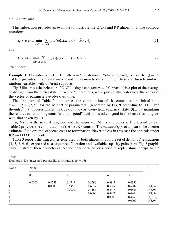
Table 1Example 1: Distances and probability distributions (Q"15)

Node Node Di

0 1 2 3 4 5

0 0.0000 0.8753 0.4749 0.3590 0.3813 0.43501 0.0000 0.5956 0.6517 0.5387 0.6802 U(1, 5)2 0.0000 0.1164 0.4446 0.0866 U(3, 9)3 0.0000 0.3873 0.0944 U(1, 5)4 0.0000 0.4768 U(6, 12)5 0.0000 U(3, 9)

5.3. An example

This subsection provides an example to illustrate the OAPI and RP algorithms. The compactnotations

Q(x, u, r),minu|U(x)

+x{|S

pxx{

(u)Mg(x, u,x@)#JI (x@, r)N (21)

and

Q(x, u),minu|U(x)

+x{|S

pxx{

(u)Mg(x,u,x@)#H(x@)N. (22)

are adopted.

Example 1. Consider a network with n"5 customers. Vehicle capacity is set to Q"15.Table 1 provides the distance matrix and the demands' distributions. These are discrete uniformrandom variables with di!erent supports.

Fig. 5 illustrates the behavior of OAPI, using a constant ct"0.01: part (a) is a plot of the average

cost-to-go from the initial state in each of 50 iterations, while part (b) illustrates how the values ofthe vector of parameters evolve over time.

The "rst part of Table 2 summarizes the computation of the control at the initial statex"(0, 15, ?, ?, ?, ?, ?) for the best set of parameters r generated by OAPI according to (11). Eventhough JI (x@, r) underestimates the true optimal cost-to-go from each next state, Q(x, u, r) maintainsthe relative order among controls and a `gooda decision is taken (good in the sense that it agreeswith that taken by RP).

Fig. 6 shows the nearest neighbor and the improved 2-Int static policies. The second part ofTable 2 provides the computation of the "rst RP control. The values of Q(x, u) appear to be a betterestimate of the optimal expected costs to termination. Nevertheless, in this case the controls underRP and OAPI coincide.

Table 3 reports the trajectories generated by both algorithms on the set of demands' realizationsM1, 5, 3, 9, 6N, expressed as a sequence of location and available capacity pairs (l, q). Fig. 7 graphi-cally illustrates these trajectories. Notice how both policies perform replenishment trips to the


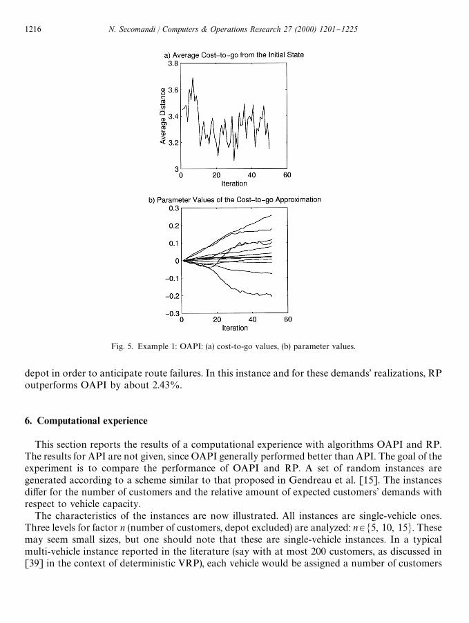
Fig. 5. Example 1: OAPI: (a) cost-to-go values, (b) parameter values.

depot in order to anticipate route failures. In this instance and for these demands' realizations, RPoutperforms OAPI by about 2.43%.

6. Computational experience

This section reports the results of a computational experience with algorithms OAPI and RP.The results for API are not given, since OAPI generally performed better than API. The goal of theexperiment is to compare the performance of OAPI and RP. A set of random instances aregenerated according to a scheme similar to that proposed in Gendreau et al. [15]. The instancesdi!er for the number of customers and the relative amount of expected customers' demands withrespect to vehicle capacity.

The characteristics of the instances are now illustrated. All instances are single-vehicle ones.Three levels for factor n (number of customers, depot excluded) are analyzed: n3M5, 10, 15N. Thesemay seem small sizes, but one should note that these are single-vehicle instances. In a typicalmulti-vehicle instance reported in the literature (say with at most 200 customers, as discussed in[39] in the context of deterministic VRP), each vehicle would be assigned a number of customers


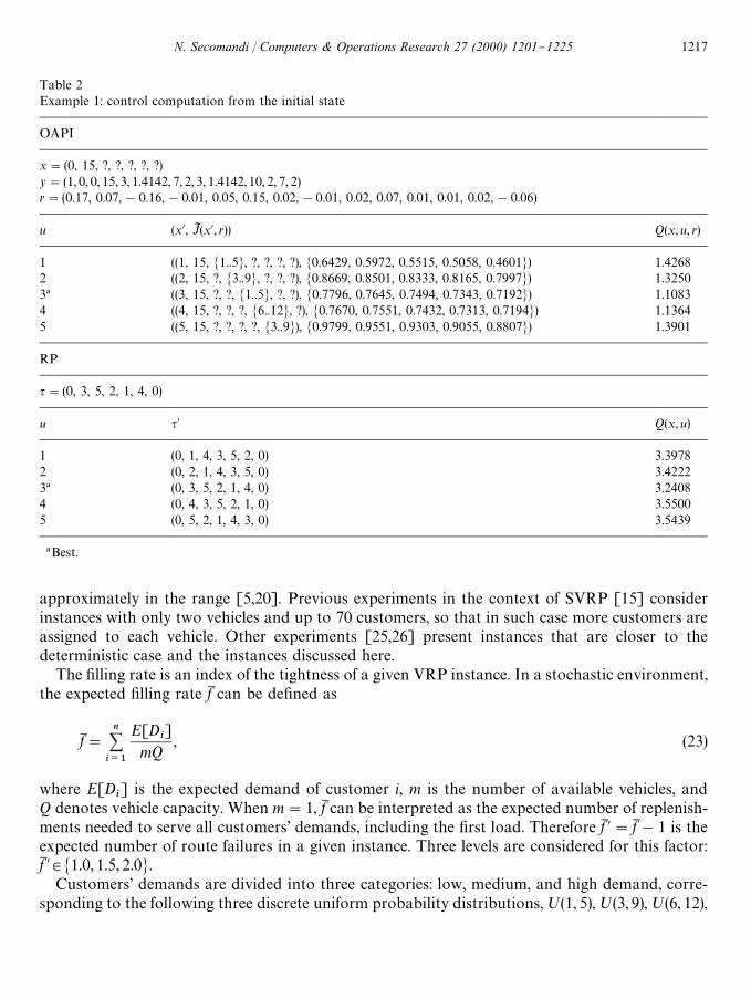
Table 2Example 1: control computation from the initial state

OAPI

x"(0, 15, ?, ?, ?, ?, ?)y"(1, 0, 0, 15, 3, 1.4142, 7, 2, 3, 1.4142, 10, 2, 7, 2)r"(0.17, 0.07,!0.16,!0.01, 0.05, 0.15, 0.02,!0.01, 0.02, 0.07, 0.01, 0.01, 0.02,!0.06)

u (x@, JI (x@, r)) Q(x, u, r)

1 ((1, 15, M1..5N, ?, ?, ?, ?), M0.6429, 0.5972, 0.5515, 0.5058, 0.4601N) 1.42682 ((2, 15, ?, M3..9N, ?, ?, ?), M0.8669, 0.8501, 0.8333, 0.8165, 0.7997N) 1.32503! ((3, 15, ?, ?, M1..5N, ?, ?), M0.7796, 0.7645, 0.7494, 0.7343, 0.7192N) 1.10834 ((4, 15, ?, ?, ?, M6..12N, ?), M0.7670, 0.7551, 0.7432, 0.7313, 0.7194N) 1.13645 ((5, 15, ?, ?, ?, ?, M3..9N), M0.9799, 0.9551, 0.9303, 0.9055, 0.8807N) 1.3901

RP

q"(0, 3, 5, 2, 1, 4, 0)

u q@ Q(x, u)

1 (0, 1, 4, 3, 5, 2, 0) 3.39782 (0, 2, 1, 4, 3, 5, 0) 3.42223! (0, 3, 5, 2, 1, 4, 0) 3.24084 (0, 4, 3, 5, 2, 1, 0) 3.55005 (0, 5, 2, 1, 4, 3, 0) 3.5439

!Best.

approximately in the range [5,20]. Previous experiments in the context of SVRP [15] considerinstances with only two vehicles and up to 70 customers, so that in such case more customers areassigned to each vehicle. Other experiments [25,26] present instances that are closer to thedeterministic case and the instances discussed here.

The "lling rate is an index of the tightness of a given VRP instance. In a stochastic environment,the expected "lling rate fM can be de"ned as

fM"n+i/1

E[Di]

mQ, (23)

where E[Di] is the expected demand of customer i, m is the number of available vehicles, and

Q denotes vehicle capacity. When m"1, fM can be interpreted as the expected number of replenish-ments needed to serve all customers' demands, including the "rst load. Therefore fM @"fM!1 is theexpected number of route failures in a given instance. Three levels are considered for this factor:fM @3M1.0, 1.5, 2.0N.

Customers' demands are divided into three categories: low, medium, and high demand, corre-sponding to the following three discrete uniform probability distributions,;(1, 5),;(3, 9),;(6, 12),


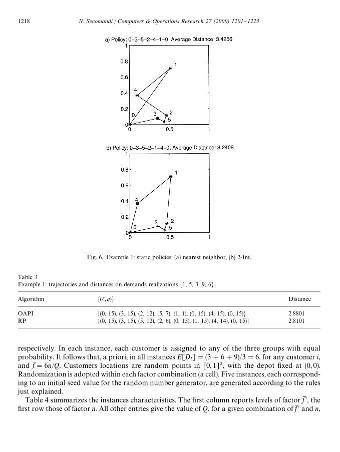
Fig. 6. Example 1: static policies: (a) nearest neighbor, (b) 2-Int.

Table 3Example 1: trajectories and distances on demands realizations M1, 5, 3, 9, 6N

Algorithm M(l,q)N Distance

OAPI M(0, 15), (3, 15), (2, 12), (5, 7), (1, 1), (0, 15), (4, 15), (0, 15)N 2.8801RP M(0, 15), (3, 15), (5, 12), (2, 6), (0, 15), (1, 15), (4, 14), (0, 15)N 2.8101

respectively. In each instance, each customer is assigned to any of the three groups with equalprobability. It follows that, a priori, in all instances E[D

i]"(3#6#9)/3"6, for any customer i,

and fM"6n/Q. Customers locations are random points in [0, 1]2, with the depot "xed at (0, 0).Randomization is adopted within each factor combination (a cell). Five instances, each correspond-ing to an initial seed value for the random number generator, are generated according to the rulesjust explained.

Table 4 summarizes the instances characteristics. The "rst column reports levels of factor fM @, the"rst row those of factor n. All other entries give the value of Q, for a given combination of fM @ and n,


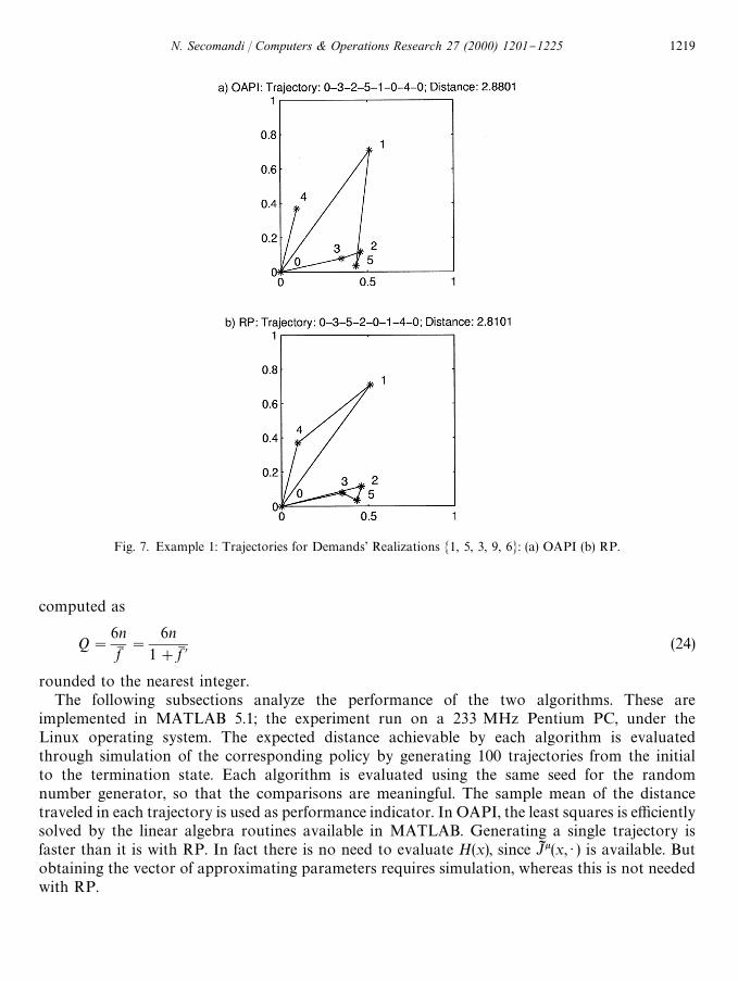
Fig. 7. Example 1: Trajectories for Demands' Realizations M1, 5, 3, 9, 6N: (a) OAPI (b) RP.

computed as

Q"

6nfM"

6n1#fM @

(24)

rounded to the nearest integer.The following subsections analyze the performance of the two algorithms. These are

implemented in MATLAB 5.1; the experiment run on a 233 MHz Pentium PC, under theLinux operating system. The expected distance achievable by each algorithm is evaluatedthrough simulation of the corresponding policy by generating 100 trajectories from the initialto the termination state. Each algorithm is evaluated using the same seed for the randomnumber generator, so that the comparisons are meaningful. The sample mean of the distancetraveled in each trajectory is used as performance indicator. In OAPI, the least squares is e$cientlysolved by the linear algebra routines available in MATLAB. Generating a single trajectory isfaster than it is with RP. In fact there is no need to evaluate H(x), since JI k(x, ) ) is available. Butobtaining the vector of approximating parameters requires simulation, whereas this is not neededwith RP.


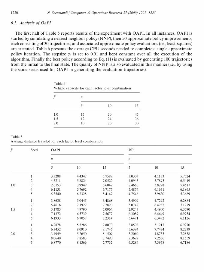
Table 5Average distance traveled for each factor level combination

fM @ Seed OAPI RP

n n

5 10 15 5 10 15

1 3.3288 4.4347 5.7589 3.0303 4.1133 5.75242 4.5211 5.8824 7.0522 4.0943 5.7893 6.5419

1.0 3 2.6153 3.9949 6.6047 2.4666 3.8278 5.45174 6.1131 5.7692 6.7177 5.4874 6.1631 6.18655 5.3540 6.2328 5.4147 4.7546 5.9630 5.3689

1 3.8638 5.0445 6.4868 3.4909 4.7292 6.28842 5.4616 7.1922 7.7820 5.0742 6.4282 7.1279

1.5 3 3.1785 4.9790 7.0964 2.9243 4.4900 6.37904 7.1372 6.5739 7.5677 6.3089 6.4649 6.97545 6.1933 6.7057 7.2314 5.6471 6.3492 6.1126

1 4.2878 5.5286 7.8073 3.8598 5.1217 6.92702 6.3452 8.0910 9.1746 5.6394 7.7434 8.2239

2.0 3 3.4949 5.2650 8.1509 3.2060 4.8733 7.28384 8.0640 7.8583 8.7490 7.3697 7.2566 8.15595 6.8770 8.1366 7.7732 6.5284 7.3958 6.7186

Table 4Vehicle capacity for each factor level combination

fM @ n

5 10 15

1.0 15 30 451.5 12 24 362.0 10 20 30

6.1. Analysis of OAPI

The "rst half of Table 5 reports results of the experiment with OAPI. In all instances, OAPI isstarted by simulating a nearest neighbor policy (NNP); then 50 approximate policy improvements,each consisting of 30 trajectories, and associated approximate policy evaluations (i.e., least-squares)are executed. Table 6 presents the average CPU seconds needed to complete a single approximatepolicy iteration. The stepsize c

tis set to 0.01 and kept constant over all the execution of the

algorithm. Finally the best policy according to Eq. (11) is evaluated by generating 100 trajectoriesfrom the initial to the "nal state. The quality of NNP is also evaluated in this manner (i.e., by usingthe same seeds used for OAPI in generating the evaluation trajectories).


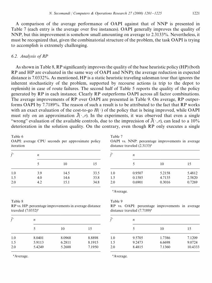
Table 8RP vs. HP: percentage improvements in average distancetraveled (7.0332)!

fM @ n

5 10 15

1.0 8.0401 8.0968 8.88981.5 5.9113 6.2811 8.19152.0 5.4249 5.2688 7.1950

!Average.

Table 9RP vs. OAPI: percentage improvements in averagedistance traveled (7.7189)!

fM @ n

5 10 15

1.0 9.5705 1.7386 7.12091.5 9.2473 6.6698 9.07242.0 8.4815 7.1360 10.4333

!Average.

Table 6OAPI: average CPU seconds per approximate policyiteration

fM @ n

5 10 15

1.0 3.9 14.5 33.51.5 4.0 14.6 33.82.0 4.2 15.1 34.8

Table 7OAPI vs. NNP: percentage improvements in averagedistance traveled (2.3133)!

fM @ n

5 10 15

1.0 0.9507 5.2158 5.48121.5 0.1585 4.7135 2.58202.0 0.6901 0.3016 0.7269

!Average.

A comparison of the average performance of OAPI against that of NNP is presented inTable 7 (each entry is the average over "ve instances). OAPI generally improves the quality ofNNP, but this improvement is somehow small amounting on average to 2.3133%. Nevertheless, itmust be recognized that, given the combinatorial structure of the problem, the task OAPI is tryingto accomplish is extremely challenging.

6.2. Analysis of RP

As shown in Table 8, RP signi"cantly improves the quality of the base heuristic policy (HP) (bothRP and HP are evaluated in the same way of OAPI and NNP); the average reduction in expecteddistance is 7.0332%. As mentioned, HP is a static heuristic traveling salesman tour that ignores theinherent stochasticity of the problem, supported by recourse actions (a trip to the depot toreplenish) in case of route failures. The second half of Table 5 reports the quality of the policygenerated by RP in each instance. Clearly RP outperforms OAPI across all factor combinations.The average improvements of RP over OAPI are presented in Table 9. On average, RP outper-forms OAPI by 7.7189%. The reason of such a result is to be attributed to the fact that RP workswith an exact evaluation of the cost-to-go H( ) ) of the policy that is being improved, while OAPImust rely on an approximation JI ( ) , r). In the experiments, it was observed that even a single`wronga evaluation of the available controls, due to the imprecision of JI ( ) , r), can lead to a 10%deterioration in the solution quality. On the contrary, even though RP only executes a single


Table 10RP: average CPU seconds per trajectory

fM @ n

5 10 15

1.0 0.3 3.5 17.51.5 0.3 3.1 15.02.0 0.3 2.8 13.6

on-line policy improvement step, it bene"ts from accurate evaluation of the controls at eachdecision point. Average CPU seconds needed to complete a single trajectory are given in Table 10.As it can be noticed, RP can be e$ciently implemented in a real-time environment. As a result, RPposes itself as a robust algorithm for SVRP. Overall, given its simplicity, its performance is quiteimpressive.

7. Conclusion

The paper presents a comparison of neuro-dynamic programming algorithms for the singlevehicle routing problem with stochastic demands. Two such algorithms are analyzed: optimisticapproximate policy iteration and a rollout policy. The computational experiment shows that therollout policy outperforms optimistic approximate policy iteration. The percentage improvementsare substantial and consistent over all the instances used in the experiment. The performance of RPis quite impressive, if one considers the simplicity of the algorithm. RP is a robust algorithm thatholds promise for a successful application to VRP business situations. (For instance, the same ideaon which RP is based can be applied to deterministic VRPs that are heuristically solved.) This doesnot seem to be the case with other `more ambitiousa and less robust neuro-dynamic programmingalgorithms, as optimistic approximate policy iteration. Further research (e.g., the use of a nonlineararchitecture for approximating the cost-to-go) and experimentation should be performed to assessthe full potential of such algorithms.

Acknowledgements

I thank Sean Curry at The MathWorks, Inc. for the excellent support provided in the use ofMATLAB. The comments and suggestions of two anonymous referees and of the guest editor led toan improved version of the original paper.

Appendix A. The expected length of a static policy

Let q"(0, 1,2, n, n#1,0) be a tour through the customers that starts and ends at the depot.Let ¸q be the random variable denoting the length of tour q. Consider the case where the vehicle is


at location l, l"0, 1,2, n, with ql denoting its currently available capacity, ql"1,2, Q. WhenlO0 it is assumed that customer l has not yet been served, so that ql represents the availablecapacity before service. If l"0, then ql,Q. Assume that some of the customers have already beenserved under an arbitrary policy. Then ql"(l, l#1,2, 0) denotes a partial tour through theremaining customers. Moreover, some of the customers may already have received a visit, so thattheir demands are known, but not completely served, perhaps because a route failure occurred. Inthis case the random variable describing the demand of each such customer is rede"ned to bea degenerate random variable assuming a value equal to the amount of pending demand withprobability 1. For notational convenience, if l"0 then D

0is assumed to be a degenerate random

variable identically equal to 0 with probability 1. Then Proposition 2 in Gendreau et al. [15] can bemodi"ed to compute E[¸q D ql], the expected length of the partial tour ql [24]:

E[¸ql D ql]"n+i/l

d(i, i#1)#al(ql), (A.1)

where an(q

n)"2d(0, n)+K

k/qn`1pn(k), for q

n"1,2, Q, and, for i"l,2, n!1, q

i"1,2, Q,

ai(q

i)"

qi~1+k/0

pi(k)a

i`1(q

i!k)

#pi(q

i)[d(i, 0!d(i, i#1)#d(0, i#1)#a

i`1(Q)]

#

K+

k/qi`1

pi(k)[2d(i, 0)#a

i`1(Q#q

i!k)]. (A.2)

The "rst term in (A.1) is the tour length if no route failures occur. The terms ai(q

i) represent the

expected extra distance traveled due to route failures before termination, given that the vehicle is atlocation i with q

iavailable capacity, and the remaining tour is q

i. The terms a

n(q

n) are the boundary

conditions. All other terms are computed by DP backward recursion by conditioning on thedemand levels of the current customer in the tour.

In a DP context, E[¸ql D ql] assumes the interpretation of a cost-to-go function, that is theexpected distance to termination, given that the current location is l, the current capacity is ql , andthe remaining portion of the tour is ql .

References

[1] Powell WB, Jaillet P, Odoni A. Stochastic and Dynamic Networks and Routing. In: Ball MO, Magnanti TL,Monma CL, Nemhauser GL, editors. Network routing, vol. 8, Handbooks in Operations Research and Manage-ment Science. Amsterdam: Elsevier, 1995 [chapter 3].

[2] Psaraftis HN. Dynamic vehicle routing. Annals of Operations Research 1995;61:143}64.[3] Bertsimas DJ, Simchi-Levi D. A new generation of vehicle routing research: robust algorithms, addressing

uncertainty. Operations Research 1996;44:286}304.[4] Bertsekas DP. Dynamic programming and optimal control. Belmont, MA: Athena Scienti"c, 1995.[5] Bertsekas DP, Tsitsiklis JN. Neuro-dynamic programming. Belmont, MA: Athena Scienti"c, 1996.[6] Sutton RS, Barto AG. Reinforcement learning. Cambridge, MA: MIT Press, 1998.[7] Golden BL, Assad AA, editors. Vehicle routing: methods and studies. Amsterdam: Elsevier, 1988.


[8] Fisher M. Vehicle routing. In: Ball MO, Magnanti TL, Monma CL, Nemhauser GL, editors. Networkrouting, Vol. 8, Handbooks in Operations Research and Management Science. Amsterdam: Elsevier, 1995[Chapter 1].

[9] Crainic TG, Laporte G. Planning models for freight transportation. European Journal of Operational Research1997;97:409}38.

[10] Bramel J, Simchi-Levi D. The logic of logistics. New York: Springer, 1997.[11] Dror M, Laporte G, Trudeau P. Vehicle routing with stochastic demands: properties and solution frameworks.

Transportation Science 1989;23:166}76.[12] Bertsimas DJ. A vehicle routing problem with stochastic demands. Operations Research 1992;40:574}85.[13] Bertsimas DJ, Chervi P, Peterson M. Computational approaches to stochastic vehicle routing problems. Transpor-

tation Science 1995;29:342}52.[14] Gendreau M, Laporte G, SeH guin R. Stochastic vehicle routing. European Journal of Operational Research

1996;88:3}12.[15] Gendreau M, Laporte G, SeH guin R. An exact algorithm for the vehicle routing problem with stochastic demands

and customers. Transportation Science 1995;29:143}55.[16] Gendreau M, Laporte G, SeH guin R. A tabu search heuristic for the vehicle routing problem with stochastic demands

and customers. Operations Research 1996;44:469}77.[17] Lambert V, Laporte G, Louveaux FV. Designing collection routes through bank branches. Computers and

Operations Research 1993;20:783}91.[18] Dror M, Ball MO, Golden BL. Computational comparison of algorithms for inventory routing. Annals of

Operations Research 1985;4:3}23.[19] Larson RC. Transportation of sludge to the 106-mile site: an inventory routing algorithm for #eet sizing and logistic

system design. Transportation Science 1988;22:186}98.[20] Bartholdi JJ, Platzman LK, Collins RL, Warden WH. A minimal technology routing system for meals on wheels.

Interfaces 1983;13:1}8.[21] Dror M. Modeling vehicle routing with uncertain demands as a stochastic program: properties of the correspond-

ing solution. European Journal of Operational Research 1993;64:432}41.[22] Bastian C, Rinnooy Kan AHG. The stochastic vehicle routing problem revisited. European Journal of Operational

Research 1992;56:407}12.[23] Yang WH, Mathur K, Ballou RH. Stochastic vehicle routing with restocking. Transportation Science, to appear.[24] Secomandi N. Exact and heuristic dynamic programming algorithms for the vehicle routing problem with

stochastic demands. Dissertation, University of Houston, USA, 1998.[25] TeodorovicH D, PavkovicH G. A simulated annealing technique approach to the vehicle routing problem in the case of

stochastic demand. Transportation Planning and Technology 1992;16:261}73.[26] Dror M, Trudeau P. Stochastic vehicle routing with modi"ed savings algorithm. European Journal of Operational

Research 1986;23:228}35.[27] Dror M, Laporte G, Louveaux FV. Vehicle routing with stochastic demands and restricted failures. Zeitschrift fuK r

Operations Research 1993;37:273}83.[28] BouzamK ene-Ayari B, Dror M, Laporte G. Vehicle routing with stochastic demands and split deliveries. Foundations

of Computing and Decision Sciences 1993;18:63}9.[29] Laporte G, Louveaux FV. The integer L-shaped method for stochastic integer programs with complete recourse.

Operations Research Letters 1993;13:133}42.[30] Golden BL, Yee JR. A framework for probabilistic vehicle routing. AIIE Transactions 1979;11:109}12.[31] Stewart WR, Golden BL. Stochastic vehicle routing: a comprehensive approach. European Journal of Operational

Research 1983;14:371}85.[32] Laporte G, Louveaux FV, Mercure H. Models and exact solutions for a class of stochastic location-routing

problems. European Journal of Operational Research 1989;39:71}8.[33] Bertsimas DJ, van Ryzin G. A stochastic and dynamic vehicle routing problem in the Euclidean plane. Operations

Research 1991;39:601}15.[34] Bertsimas DJ, van Ryzin G. Stochastic and dynamic vehicle routing in the Euclidean plane with multiple

capacitated vehicles. Operations Research 1993;41:60}76.


[35] Bertsimas DJ, van Ryzin G. Stochastic and dynamic vehicle routing with general demand and interarrival timedistributions. Advances in Applied Probability 1993;25:947}78.

[36] Bertsekas DP, Tsitsiklis JN, Wu C. Rollout algorithms for combinatorial optimization. Journal of Heuristics1997;3:245}62.

[37] Bertsekas DP, Castanon DA. Rollout algorithms for stochastic scheduling problems. Journal of Heuristics,to appear.

[38] Nemhauser GL, Wolsey LA. Integer and combinatorial optimization. New York: Wiley, 1988.[39] Gendreau M, Hertz A, Laporte G. A tabu search heuristic for the vehicle routing problem. Management Science

1994;40:1276}90.

Nicola Secomandi received his Ph.D. degree in operations research from the University of Houston in 1998. He is nowa research scientist in the R&D department of PROS Strategic Solutions, a Houston based company that specializesin the application of revenue management. His current research interests involve stochastic and dynamic transportationproblems, rollout algorithms, metaheuristics, "nancial engineering, and the theory and applications of revenuemanagement, in particular as it applies to the energy industry.


Comparing neuro-dynamic programming algorithms for...

Documents

Transcript of Comparing neuro-dynamic programming algorithms for...