Comparing Group Means using Regression - The … · Web viewCompute a product variable, the product...

Lecture 12: ANCOVA, Cross Validation, Dominance

Analysis of Covariance

Analysis of covariance is any analysis involving a qualitative/categorical/nominal research factor and one or more quantitative predictors in which . . .

1) the interest of the researcher is on differences in means of groups defined by the categorical variable and for that reason

2) the quantitative predictors are merely included as controlling variables.

So ANCOVA, as it’s called, is simply regression analysis involving qualitative and quantitative IVs with an attitude – a focus on the significance of differences associated with qualitative factors while controlling for quantitative variables.

Scenario. You’ve compared means of three groups using the analysis of variance. Someone suggests that you “run an analysis of covariance.” What does that mean?

It probably means that you should add quantitative predictors to the analysis and assess the significance of the differences between the three groups while controlling for those quantitative variables.

The standard procedure that is followed to conduct analysis of covariance or any analysis involving both qualitative and quantitative IVs is as follows

0. Compute a product variable, the product of the qualitative and quantitative research factors.

1. Perform a regression analysis involving the qualitative factor only, not controlling for the quantitative factor.

If the qualitative factor is dichotomous, this is just a simple regression. In such a case, you can even get the essential significance results from inspection of a correlation matrix.

If the qualitative factor has 3 or more levels, you’ll have to group-code them with K-1 group-coding variables and run a multiple regression.

The results of this analysis tell you whether the differences between the means of the groups are significant or not without controlling for the covariates.

2. Add the quantitative factor to the analysis and perform a multiple regression of Y onto both the qualitative factor(s) and the quantitative factor. Record the results.

3. Add the product of qualitative and quantitative factors and perform a third regression - of Y onto the qualitative, quantitative, and product variables. (Keep your fingers crossed that the product is NS.)

4. If the product term is significant in analysis 3 above, interpret the analysis 3 equation. If it is not significant – meaning there is no interaction of qualitative and quantitative factors go to Step 5.

5. IF the quantitative predictor is significant, Interpret the Analysis 2 equation, otherwise Interpret the Analysis 1 equation..

Lecture 12_ANCOVA - 1 5/6/2023

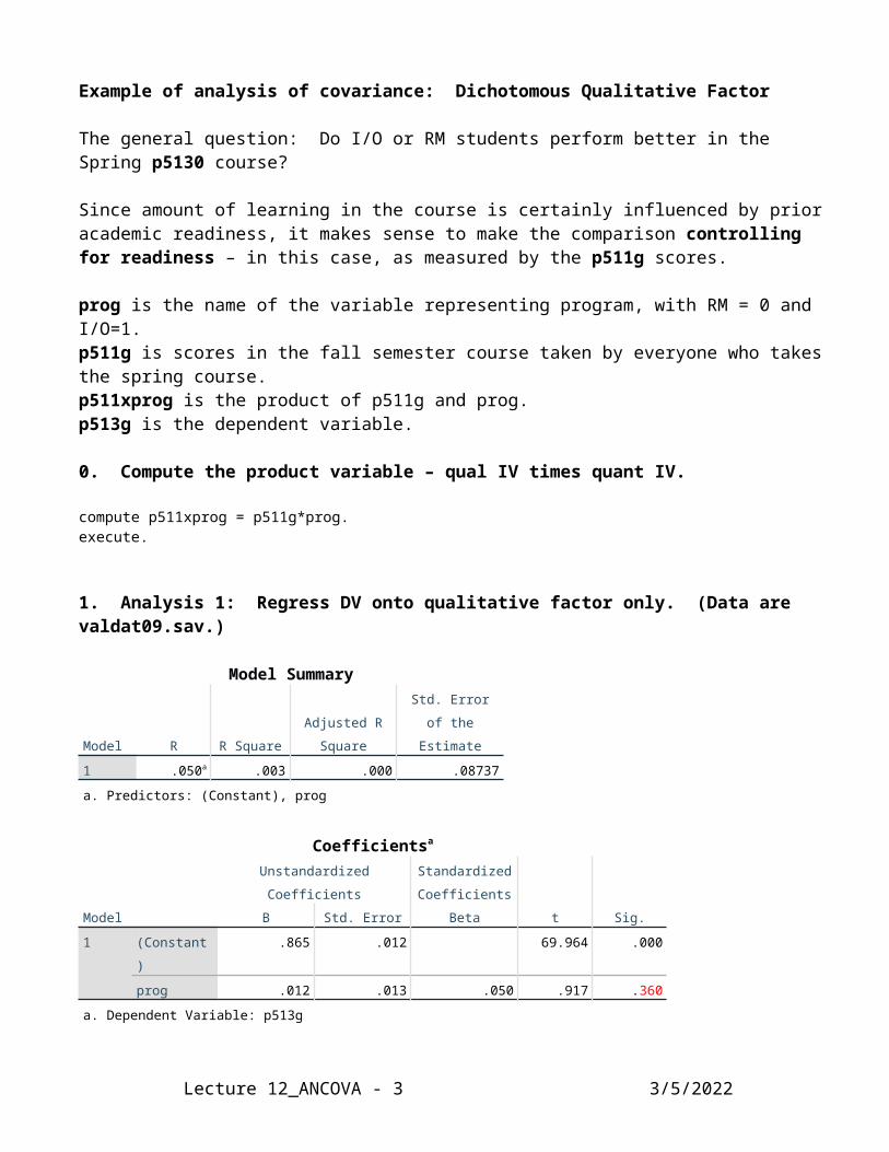
Example of analysis of covariance: Dichotomous Qualitative Factor

The general question: Do I/O or RM students perform better in the Spring p5130 course?

Since amount of learning in the course is certainly influenced by prior academic readiness, it makes sense to make the comparison controlling for readiness – in this case, as measured by the p511g scores.

prog is the name of the variable representing program, with RM = 0 and I/O=1.p511g is scores in the fall semester course taken by everyone who takes the spring course.p511xprog is the product of p511g and prog. p513g is the dependent variable.

0. Compute the product variable – qual IV times quant IV.

compute p511xprog = p511g*prog.execute.

1. Analysis 1: Regress DV onto qualitative factor only. (Data are valdat09.sav.)

Model Summary

Model R R Square

Adjusted R

Square

Std. Error of the

Estimate

1 .050a .003 .000 .08737

a. Predictors: (Constant), prog

Coefficientsa

Model

Unstandardized Coefficients

Standardized

Coefficients

t Sig.B Std. Error Beta

1 (Constant) .865 .012 69.964 .000

prog .012 .013 .050 .917 .360

a. Dependent Variable: p513g

The uncontrolled difference between I-O and RM p513g means is not significant.

Now we must see if this difference holds up when we control for any possible differences in p511g scores.


2. Analysis 2: Regression of DV onto both the qualitative and quantitative factors.

I can do this easily in REGRESSION since prog is a dichotomy.

Model Summary

Model R R Square

Adjusted R

Square

Std. Error of the

Estimate

1 .731a .535 .532 .05976

a. Predictors: (Constant), p511g, prog

Coefficientsa

Model


Standardized

Coefficients


1 (Constant) .112 .039 2.848 .005

prog .023 .009 .094 2.527 .012

p511g .849 .043 .731 19.548 .000


OMG!!! There IS a difference in mean p513g performance between the two programs among persons equal in p511g scores.

Among persons equal in p511g scores, the mean I-O performance in p513g was slightly but significantly higher than mean RM performance.

Before interpreting this analysis, however, we must perform analysis #3, looking for an interaction of NEWFORM and PROG. It’s possible, for example, that the differences between programs may vary depending on the level of performance in p511g.

This would be revealed in a significant interaction (i.e., product) term.


Prog

0 1

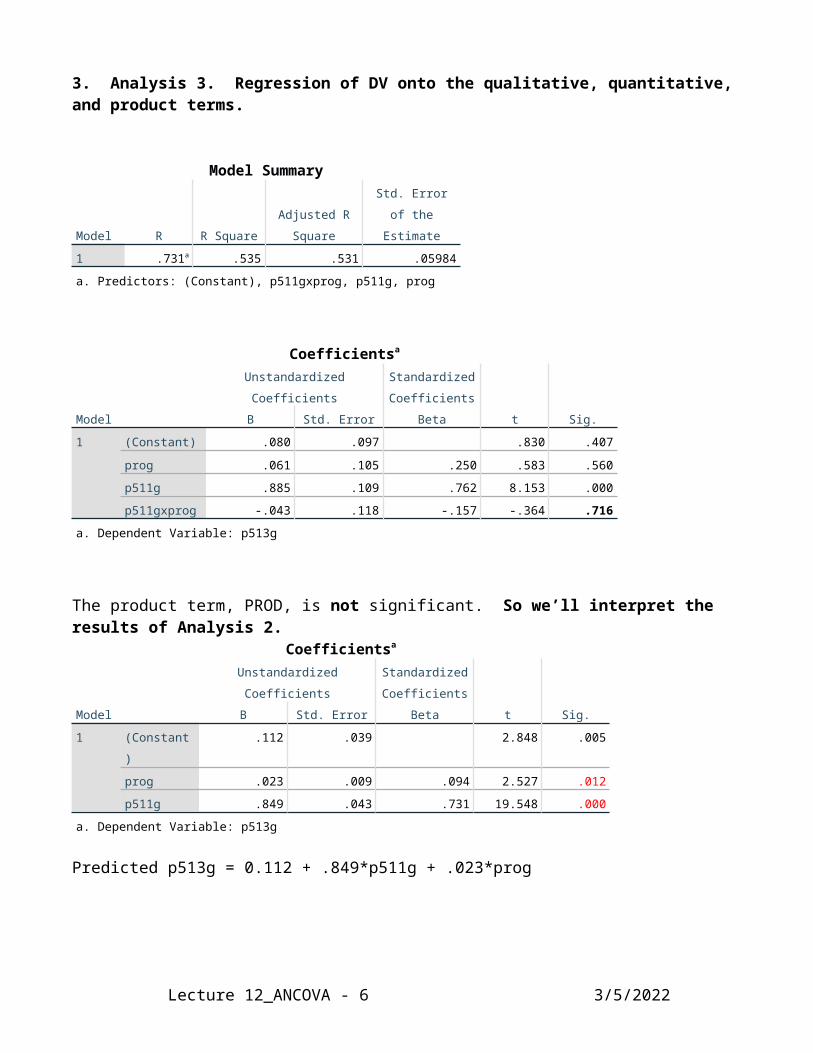
3. Analysis 3. Regression of DV onto the qualitative, quantitative, and product terms.

Model Summary

Model R R Square

Adjusted R

Square

Std. Error of the

Estimate

1 .731a .535 .531 .05984

a. Predictors: (Constant), p511gxprog, p511g, prog

Coefficientsa

Model


Standardized

Coefficients


1 (Constant) .080 .097 .830 .407

prog .061 .105 .250 .583 .560

p511g .885 .109 .762 8.153 .000

p511gxprog -.043 .118 -.157 -.364 .716


The product term, PROD, is not significant. So we’ll interpret the results of Analysis 2.Coefficientsa

Model


Standardized

Coefficients


1 (Constant) .112 .039 2.848 .005

prog .023 .009 .094 2.527 .012

p511g .849 .043 .731 19.548 .000


Predicted p513g = 0.112 + .849*p511g + .023*prog

So we would expect an I-O student and a RM student with equal p511g scores to differ by .023in their p513g proportion of total possible points – the I-O student would be roughly .023 points higher.

I should point out that this analysis was based on data gathered prior to 2009, years ago.


Graphing the results

The lines though each point are nearly parallel, as indicated by the lack of significance of the product term. There are 3 students, all RM, who did much worse than predicted by their p511g scores. Clearly those three students, as a group, “dragged down” the RM regression line.


Analysis of Covariance Comparing 3 groups

This analysis is a Manipulation Check on Raven Worthy’s thesis data

Raven’s design was a 3 between subjects x 2 repeated measures design.

She had 3 groups of participantsTime 1 Time 2

Group 1: Honest instructions on Website 1 Honest instructions on Website 2Responded to Big 5 Questionnaire Responded to Big 5 Questionnaire

Group 2: Honest instructions on Website 1 Instructions to fake good on Website 2Responded to Big 5 Questionnaire Responded to Big 5 Questionnaire

Group 3: Honest instructions on Website 1 Incentives to fake good on Website 2Responded to Big 5 Questionnaire Responded to Big 5 Questionnaire

The question here is the following: Did the instructions lead to differences in conscientiousness scores – larger mean scores in the faking conditions than in the honest condition? We expected higher scores in the Instructions-to-fake and the Incentives-to-fake conditions than in the honest condition.

Because the incentive manipulation was weak, we actually expected the following differences:

Honest Mean < Incentive Mean < Faking Mean.

A natural covariate is Website 1 honest condition conscientiousness scores. If there were differences between conditions in actual conscientiousness, then those differences should be controlled for when comparing conscientiousness scores after the instructional manipulation.

So, to summarize

Dependent variable: Conscientiousness scores obtained from Website 2 (coth).

Qualitative research factor: Instructional condition (ncondit) with 3 levels

Covariate: Website 1 honest condition responses on a separate Big Five Conscientiousness scale (corig)

Expectation: When controlling for conscientiousness as measured from the Website 1 Questionnaire, mean conscientiousness will be greatest in the instructed faking condition.

We’ll analyze Conscientiousness scores only, since C is the dimension we’re most interested in.

Because I’m too lazy to dummy code the 3 conditions, I’ll use GLM for all the analyses.


Step 0. Compute the product variable. GLM will do that for us.Step 1. Qualitative factor only.

UNIANOVA coth BY ncondit /METHOD=SSTYPE(3) /INTERCEPT=INCLUDE /POSTHOC=ncondit(BTUKEY) /PLOT=PROFILE(ncondit) /PRINT=OPOWER ETASQ DESCRIPTIVE /CRITERIA=ALPHA(.05) /DESIGN=ncondit.

Univariate Analysis of Variance

[DataSet1] G:\MDBR\0DataFiles\Rosetta_CompleteData_110911.sav

Between-Subjects FactorsN

ncondit

1 110

2 108

3 110

Descriptive StatisticsDependent Variable: coth

ncondit Mean Std. Deviation N

1 4.8211 .97555 1102 5.6404 1.07718 1083 5.1264 .93227 110Total 5.1933 1.04917 328

Tests of Between-Subjects EffectsDependent Variable: coth

Source Type III Sum of Squares

df Mean Square F Sig. Partial Eta Squared

Noncent. Parameter

Observed Powerb

Corrected Model 37.321a 2 18.661 18.798 .000 .104 37.596 1.000Intercept 8854.796 1 8854.796 8919.973 .000 .965 8919.973 1.000ncondit 37.321 2 18.661 18.798 .000 .104 37.596 1.000

Error 322.625 325 .993

Total 9206.170 328

Corrected Total 359.946 327

a. R Squared = .104 (Adjusted R Squared = .098)b. Computed using alpha = .05


Effect size 1: (5.64 – 4.82)/1.02 = .8Effect size 2: (5.13 – 4.82)/0.95 = .3

Post Hoc Tests – without the covariateOfficial Condition variable: 1=H, 2=F, 3=In(centive)

nconditHomogeneous Subsets

cothTukey B

ncondit N Subset

1 2 3

1 110 4.8211

3 110 5.1264

2 108 5.6404

Means for groups in homogeneous subsets are displayed. Based on observed means. The error term is Mean Square(Error) = .993.a. Uses Harmonic Mean Sample Size = 109.325.b. The group sizes are unequal. The harmonic mean of the group sizes is used. Type I error levels are not guaranteed.c. Alpha = .05.

Profile Plots

So, there were between condition differences in C scores, with the greatest amount of faking in the “Fake Good” condition, the next in the condition with incentives to fake, and the least amount in the honest response condition, as expected.

The next question is: Will these differences hold up when controlling for differences in Conscientiousness, as measured by a different scale?


H F In

Step 2. Adding the covariate.

UNIANOVA coth BY ncondit with corig /METHOD=SSTYPE(3) /INTERCEPT=INCLUDE /POSTHOC=ncondit(BTUKEY) /PLOT=PROFILE(ncondit) /PRINT=OPOWER ETASQ DESCRIPTIVE /CRITERIA=ALPHA(.05) /DESIGN=ncondit corig.

Univariate Analysis of Variance

[DataSet1]

G:\MDBR\0DataFiles\Rosetta_CompleteData_110911.sav

WarningsThe POSTHOC subcommand will be ignored because there are covariates in the design.

Descriptive Statistics

Dependent Variable: coth

ncondit Mean Std. Deviation N

1 4.8211 .97555 110

2 5.6404 1.07718 108

3 5.1264 .93227 110

Total 5.1933 1.04917 328




Noncent. Parameter

Observed Powerb

Corrected Model 148.239a 3 49.413 75.622 .000 .412 226.867 1.000Intercept 40.750 1 40.750 62.364 .000 .161 62.364 1.000ncondit 44.158 2 22.079 33.790 .000 .173 67.580 1.000corig 110.918 1 110.918 169.750 .000 .344 169.750 1.000

Error 211.707 324 .653

Total 9206.170 328



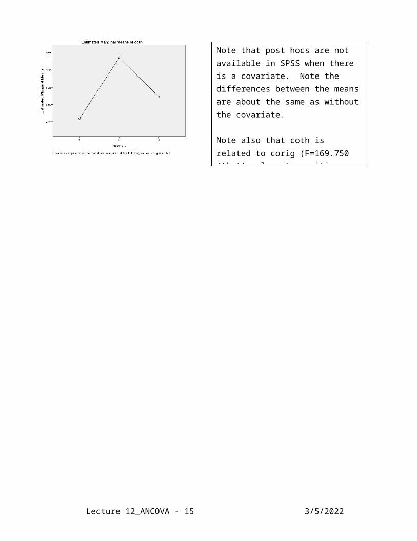
Profile Plots


Really??? Come on SPSS, get with it!


Note that post hocs are not available in SPSS when there is a covariate. Note the differences between the means are about the same as without the covariate.

Note also that coth is related to corig (F=169.750 (that’s close to positive infinity), p << .001). Differences in conscientiousness between individuals were pretty consistent across instructional conditions.

Step 3. Checking for moderation.

Add interaction terms to the equation by clicking on the [Model] button and then choosing Custom analysis.

Then, create the following product terms . .

A. Click on Custom.

B. Move ncondit and

corig to Model: field

C. Move ncondit*corig

to Model: field


The output . . .

UNIANOVA coth BY ncondit WITH corig /METHOD=SSTYPE(3) /INTERCEPT=INCLUDE /PRINT=OPOWER ETASQ DESCRIPTIVE /CRITERIA=ALPHA(.05) /DESIGN=ncondit corig corig*ncondit.




Noncent. Parameter

Observed Powerb

Corrected Model 158.098a 5 31.620 50.441 .000 .439 252.206 1.000Intercept 41.096 1 41.096 65.559 .000 .169 65.559 1.000ncondit 18.599 2 9.300 14.835 .000 .084 29.671 .999corig 106.907 1 106.907 170.543 .000 .346 170.543 1.000ncondit * corig 9.859 2 4.929 7.863 .000 .047 15.727 .952

Error 201.849 322 .627

Total 9206.170 328



Argh!! The product term is significant. This means that the differences between the means are not the same at different levels of the covariate.

So, what should we do?

In such cases, I often categorize the covariate and perform separate analyses for each category, in order to visualize how the differences between means change across different levels of the covariate.

So I dichotomized the corig variable at the median, forming two groups . . .

1. A high conscientiousness group, and2. A low conscientiousness group.


Here’s what I found . . .

For the group with lowest corig, i.e., lowest conscientiousness as measured by the first questionnaire - Post Hoc TestsnconditHomogeneous Subsets

cothTukey B

ncondit N Subset

1 2 3

1 61 4.2463

3 54 4.7130

2 63 5.4185


For the group with highest corig –Post Hoc TestsnconditHomogeneous Subsets

cothTukey B

ncondit N Subset

1 2

3 56 5.5250

1 49 5.5367

2 45 5.9511


So, among person with highest conscientiousness, based on the responses to the scale on Website 1, there was no difference between the average conscientiousness of the honest and the incentive conditions.

It may be that persons with high conscientiousness don’t fake unless instructed to.

Hmm.


H Ins Inc

CROSS VALIDATION – start here on 4/17/18The need for cross validation

Prediction in new samples. Often, we'll want to use the regression coefficients obtained from the sample in our study to predict y's for new persons sampled from the same population as the persons upon whom the original regression analysis was performed.

Since they're from the same population, at first glance it would seem that there should be no trouble in applying the regression coefficients obtained from the original sample to predict y-values for new persons. Wrong.

The problem lies with the fact that the regression coefficients estimated from the persons included in a multiple regression analysis depend on two factors. . .

1. The true relationship which exists in the population. Of course, if the new people are from the same population as the original, this will present no problem.

2. Errors of measurement specific to the particular sample upon which the original multiple regression was based. This is the problem.

Although new people may be from the same population as the original upon which the original regression was based, specific vagaries of our original sample will not be applicable to them – the particular mix of people, the thoughts respondents had when filling out the questionnaire, what the president tweeted the morning the questionnaire was responded to are all things which make each sample different from every other sample.

So, the regression coefficients obtained from a sample, may be quite different from what they should be (in the population) due to the specific random characteristics of the sample upon which the analysis was based. This should not be news to you. Remember the discussion last semester on the sampling distribution of the mean. That’s the same issue.

The need for meta-analysis is a related phenomenon. If relationships were immune to sample specifics – errors of measurement – there would be no need for meta-analysis. The examples presented in last semester’s meta-analysis lecture show that pretty much everything changes from one sample to the next.

The issue is: Are the sample-specific differences are so big that they prevent us from doing our job – predicting performance or assessing relationships?

Cross-validation provides evidence regarding that question.


Cross validation to the rescue

A way of protecting yourself against such a potentially embarrassing situation is to take two samples. (or take one big one and divide it in half.)

Perform the regression analysis on one. Call this sample the validation sample.

Then use the coefficients computed from the first to generate predicted y's using the data of the second sample. Call the second sample the holdout sample.

In the holdout sample compute the R between predicted Ys computed using the validation sample regression coefficients and the holdout sample actual Ys.

If the holdout R is not too much smaller than that from the R obtained in the validation sample, then you can have confidence in predictions of individual y values on new persons from the same population.

However, if the R in the holdout sample is too much shrunken from the original multiple R in the validation sample, then you should be quite wary of using the regression weights obtained from the validation sample.


Visually


Holdout Sample

Compute Y-hats using validation sample regressioncoefficients.

Correlate these Y-hats with observed Ys.

Record this correlation.

Validation Sample

Multiple regressionto get regression coefficients.

Multiple R recorded.

Comparison

Correlations (or R2's) from the two samples compared.

No shrinkage: Keep coefficients.

Shrinkage: Rethink problem

Cross Validation Example 1

The following is an example of cross validation of an equation predicting grade point average from Wonderlic Personnel Test (WPT) and Conscientiousness scale scores from the 50-item IPIP sample Big Five questionnaire.

1. Form Validation and Holdout Samples.

compute sample = 1.if (expnum/2 = trunc(expnum/2)) sample = 2.

frequencies variables=sample.

Frequencies [DataSet1] G:\MDBR\0DataFiles\Rosetta_CompleteData_110911.sav

Statisticssample

NValid 328

Missing 0

sampleFrequency Percent Valid Percent Cumulative Percent

Valid

1.00 165 50.3 50.3 50.3

2.00 163 49.7 49.7 100.0

Total 328 100.0 100.0

value labels sample 1 "Validation" 2 "Holdout".


This statement puts each case whose expnum is an even number into Sample 2.

2. Perform Regression of Criterion onto predictors in Validation sample and record regression coefficients and R.

temporary.select if (sample = 1). (Sample 1 is the Validation Sample.)

regression variables = eoygpa corig wpt /dep=eoygpa /enter.

Regression [DataSet1] G:\MDBR\0DataFiles\Rosetta_CompleteData_110911.sav

Variables Entered/Removeda

Model Variables Entered Variables Removed Method

1 wpt, corigb . Enter

a. Dependent Variable: EOYGPA

b. All requested variables entered.

Model Summary

Model R R Square Adjusted R Square Std. Error of the Estimate

1 .324a .105 .094 .6661

a. Predictors: (Constant), wpt, corig

Coefficientsa

Model Unstandardized Coefficients Standardized Coefficients

t Sig.

B Std. Error Beta

1

(Constant) 1.399 .388 3.602 .000

corig .116 .058 .150 1.996 .048

wpt .043 .011 .307 4.100 .000

a. Dependent Variable: EOYGPA

3. In Holdout sample compute Y-hats from Validation sample regression coefficients and correlate them with Holdout sample observed Ys.temporary.select if (sample = 2).

compute yhat = 1.399 + 0.116*corig + .0432*wpt.

correlation yhat with eoygpa.

Correlations [DataSet1] G:\MDBR\0DataFiles\Rosetta_CompleteData_110911.sav

CorrelationsEOYGPA

yhat

Pearson Correlation .313

Sig. (2-tailed) .000

N 163

4. Compare the correlations.

.324 from the Validation sample is about equal to .313 from the Holdout sample.So the regression cross validates.


Cross-validation Example 2

In a recently submitted article, we had HEXACO personality questionnaire + GPA data from two samples.

Validation Sample

In the Validation Sample, N = 770. Data were gathered in Spring 2016-Fall 2016.Participants took the 100-item HEXACO questionnaire. The 60 items in that questionnaire that make up the HEXACO-60 were analyzed.

Factor scores representing each HEXACO domain – Honesty/Humility, Emotionality, eXtraversion, Agreeableness, Conscientiousness, and Openness – along with an affect composite extracted through factor analysis were the predictors of GPA.

The results of the Multiple Regression Analysis for Sample 1, the Validation Sample were

Standardized Partial Regression Coefficients for Validation Sample

Hon/ Coeffiients Cons Hum Emot eXt Agr Con Opn Affect Multiple RStandardized 0 .025 .066 -.023 -.070 .190 -.021 .189 .299

Raw 3.037 .024 .055 -.019 -.061 .163 -.017 .268 .299

For cross-validation, the only value in the above table that is important is the Multiple R of .299. But the point of our paper is that there it is possible to measure affective state from the HEXACO and use it as a predictor of other variables. In this particular instance, the affect predictor is 2nd best which supports our belief that this “extra” characteristic measured from the HEXACO is important.

Holdout sample

N = 1597. Data were gathered from Spring 2014 through Spring 2016.

Regression equation, from SPSS. compute yhatfor5130 = 3.037 - .019*hx60esemtrocrmmpmnGTR1 - .061*ha60esemtrocrmmpmnGTR1 + .163*hc60esemtrocrmmpmnGTR1 - .055*hs60esemtrocrmmpmnGTR1 - .017*ho60esemtrocrmmpmnGTR1 + .024*hh60esemtrocrmmpmnGTR1 + .268*hmean60esemtrocrmmpmnGTR1.

Note: The computation is based on RAW partial regression coefficients, not the standardized coefficients shown above.

Correlationsyhatfor5130

eosgpa1 EOS GPA of Semester of 1st Participation including transfer gpa

Pearson Correlation .280Sig. (2-tailed) .000N 1597

This example suggests that the regression coefficients obtained from the validation sample are applicable in the holdout sample


Determining predictor importance

Candidates for predictor importance measures

1. Simple correlations.

But they’re contaminated by relationship with other variables.

2. Standardized Regression Coefficients – the Beta weights.

Become problematic when predictors are highly correlated.

3. Part r2s.

Used by themselves, they’re somewhat useful. They form the basis for what follows.

Dominance analysis

Suppose you have K predictors of a dependent variable.

Dominance analysis measures predictor importance by averaging

a. squared simple correlationsb. squared part correlations controlling for 1 other predictorc. squared part correlations controlling for 2 other predictors...k. squared part correlations controlling for all K-1 other predictors.

The measure of dominance is the average of a variable’s simple r2, squared part rs controlling for each single other predictor, squared part rs controlling for all pairs of other predictors, . . . squared part r controlling for all K-1 other predictors.


Example

Consider the prediction of P513G by UGPA, GREV, and GREQ. Here’s the SPSS output that was used to complete the table below.

First, consider all simple correlations between the criterion and predictors. These are also called zero-order correlations.

Correlationsp513g ugpa grev greq

Pearson Correlation p513g 1.000 .298 .171 .382

ugpa .298 1.000 .074 -.077

grev .171 .074 1.000 .258

greq .382 -.077 .258 1.000

Mike – The data are all cases not missing on p513g, ugpa, grev, and greq from Valdat2008.


This table is for the squared simple correlations – controlling for 0 other variables.

Next, conduct all possible two-predictor regressions. These results are in Models 1, 3, & 5 below.Models 1, 3, 5 are two predictor equations. So, the part correlations in each of these rows control for one of the other variables.

The syntax for this isregression variables = p513g ugpa grev greq /des=corr /sta=default zpp /dep=p513g /enter ugpa grev.regression variables = p513g ugpa grev greq /des=corr /sta=default zpp /dep=p513g /enter ugpa greq.regression variables = p513g ugpa grev greq /des=corr /sta=default zpp /dep=p513g /enter grev greq.

The part correlations areCoefficientsa

Model


Standardized Coefficients

t Sig.Correlations

B Std. Error Beta Zero-order Partial Part1 (Constant) .562 .054 10.470 .000

ugpa .072 .014 .287 5.121 .000 .298 .291 .286grev .000 .000 .150 2.671 .008 .171 .157 .149


Coefficientsa

Model



t Sig.Correlations


ugpa .082 .013 .330 6.415 .000 .298 .356 .329greq .000 .000 .408 7.933 .000 .382 .426 .406


Coefficientsa

Model



t Sig.Correlations


grev 8.691E-5 .000 .078 1.376 .170 .171 .081 .075greq .000 .000 .362 6.407 .000 .382 .355 .350


Next, conduct all possible three-predictor regressions. There is only 1.regression variables = p513g ugpa grev greq /des=corr /sta=default zpp /dep=p513g /enter ugpa grev greq.

The part correlations areCoefficientsa

Model



t Sig.Correlations


ugpa .081 .013 .325 6.298 .000 .298 .351 .323grev 5.028E-5 .000 .045 .844 .399 .171 .050 .043greq .000 .000 .396 7.422 .000 .382 .404 .380



The computation worksheet –

Predictor: UGPA GREV GREQ

Simple rs .298 .171 .382

Two-predictor Part rs .286 .149 .406.329 .075 .350

Three-predictor Part r .323 .043 .380

Simple r-squareds .089 .029 .146

Two-predictor Part r2s .082 .022 .165.108 .006 .122

Three-predictor Part-r2s .104 .002 .144

Mean of Simple r2s .089 .029 .146

Mean of two-predictor Part r2s .095 .014 .144

Mean of three-predictor Part r2s .104 .002 .144

Mean of all levels .096 .015 .145

These agree with the Raw Relative Weights computed using the web site on the following page . . .

> #R-squared For the Model> RSQ.Results[1] 0.2561579> > #The Raw and Rescaled Weights> RW.Results Variables Raw.RelWeight Rescaled.RelWeight1 grev 0.01444301 5.6383252 greq 0.14543058 56.7738123 ugpa 0.09628427 37.587863

This analysis suggests that GREQ was the most important predictor of P513 grades, UGPA contributed somewhat to prediction of P513G, and GREV predicted very little.

This is one form of dominance analysis. There are variations on this in the dominance analysis literature.


Dominance Analysis / Relative Importance Analysis Reference

Tonidandel, S., & LeBreton, J. M. (2015). RWA web: A free, comprehensive, web-based, and user-friendly tool for relative weight analyses. Journal of Business and Psychology, volume 30, 2, 207-215 http://relativeimportance.davidson.edu

This is the article featuring the above web page.

You may have to inspect the csv file containing the data to make sure that it uses Windows Default encoding and that there are no “garbage” characters in the names. I found them in the very first name in the file. The R code won’t work unless the variable names are what you’ve said they would be.


Comparing Group Means using Regression - The … · Web viewCompute a product variable, the product...

Documents

Transcript of Comparing Group Means using Regression - The … · Web viewCompute a product variable, the product...