Comparing Density Forecasts via Weighted Likelihood

Ratio Tests�

Gianni Amisanoyand Ra¤aella Giacominiz

University of Brescia, Italy and University of California, Los Angeles

This version: February 2005

Abstract

We propose a test for comparing the out-of-sample accuracy of competing density forecasts

of a variable. The test is valid under general conditions: the data can be heterogeneous and

the forecasts can be based on (nested or non-nested) parametric models or produced by semi-

parametric, non-parametric or Bayesian estimation techniques. The evaluation is based on scoring

rules, which are loss functions de�ned over the density forecast and the realizations of the variable.

We restrict attention to the logarithmic scoring rule and propose an out-of-sample �weighted

likelihood ratio�test that compares weighted averages of the scores for the competing forecasts.

The user-de�ned weights are a way to focus attention on di¤erent regions of the distribution of

the variable. For a uniform weight function, the test can be interpreted as an extension of Vuong

(1989)�s likelihood ratio test to time series data and to an out-of-sample testing framework. We

apply the tests to evaluate density forecasts of US in�ation produced by linear and Markov

Switching Phillips curve models estimated by either maximum likelihood or Bayesian methods.

We conclude that a Markov Switching Phillips curve estimated by maximum likelihood produces

the best density forecasts of in�ation.

�We are deeply indebted to Clive W. J. Granger for many interesting discussions. We also thank Carlos Capistran,

Roberto Casarin, Graham Elliott, Ivana Komunjer, Andrew Patton, Kevin Sheppard, Allan Timmermann and seminar

participants at the University of Brescia for valuable comments. This paper was previously circulated under the title

"Comparing Density Forecasts via Weighted Likelihood Ratio Tests: Asymptotic and Bootstrap Methods", by Ra¤aella

Giacomini.yamisano@eco.unibs.itzgiacomin@econ.ucla.edu

1

1 Introduction

A density forecast is an estimate of the future probability distribution of a random variable, condi-

tional on the information available at the time the forecast is made. It thus represents a complete

characterization of the uncertainty associated with the forecast, as opposed to a point forecast, which

provides no information about the uncertainty of the prediction.

Density forecasting is receiving increasing attention in both macroeconomics and �nance (see

Tay and Wallis, 2000 for a survey). A famous example of density forecasting in macroeconomics

is the �fan-chart� of in�ation and GDP published by the Bank of England and by the Sveriges

Riksbank in Sweden in their quarterly In�ation Reports (for other examples of density forecasting

in macroeconomics, see also Diebold, Tay and Wallis, 1999 and Clements and Smith, 2000). In

�nance, where the wide availability of data and the increasing computational power make it possible

to produce more accurate estimates of densities, the examples are numerous. Leading cases are in

risk management, where forecasts of portfolio distributions are issued with the purpose of tracking

measures of portfolio risk such as the Value-at-Risk (see, e.g., Du¢ e and Pan, 1996) or the Expected

Shortfall (see, e.g., Artzner et al., 1997). Another example is the extraction of density forecasts

from option price data (see, e.g. Soderlind and Svensson, 1997). The vast literature on forecasting

volatility with GARCH-type models (see Bollerslev, Engle and Nelson, 1994) and its extensions to

forecasting higher moments of the conditional distribution (see Hansen, 1994) can also be seen as

precursors to density forecasting. The use of sophisticated distributions for the standardized residuals

of a GARCH model and the modeling of time dependence in higher moments is in many cases an

attempt to capture relevant features of the data to better approximate the true distribution of the

variable. Finally, in the multivariate context, a focus on densities is the central issue in the literature

on copula modeling and forecasting, that is gaining interest in �nancial econometrics (Patton, 2001).

With density forecasting becoming more and more widespread in applied econometrics, it is

necessary to develop reliable techniques to evaluate the forecasts�performance. The literature on

evaluation of density forecasts (or, equivalently, predictive distributions) is still young, but growing

at fast speed. In one of the earliest contributions, Diebold, Gunther and Tay (1998) suggested eval-

uating a sequence of density forecasts by assessing whether the probability integral transforms of

the realizations of the variable with respect to the forecast densities are independent and identically

distributed (i.i.d.) U(0; 1): While Diebold et al. (1998) adopted mainly qualitative tools for testing

the i.i.d. U(0; 1) behavior of the transformed data, formal tests of the same hypothesis have been

suggested by Berkowitz (2001), Hong and White (2000), Hong (2001). Tests that account for parame-

ter estimation uncertainty have been proposed by Hong and Li (2001), Bai (2003) and Corradi and

Swanson (2003) (the latter further allowing for dynamic misspeci�cation under the null hypothesis).

It is important to emphasize that the above methods focus on absolute evaluation, that is, on

evaluating the �goodness� of a given sequence of density forecasts, relative to the data-generating

2

process. In practice, however, it is likely that any econometric model used to produce the sequence

of density forecasts is misspeci�ed, and an absolute test will typically give no guidance to the user

as to what to do in case of rejection. In this situation a more practically relevant question is how to

decide which of two (or more) competing density forecasts is preferable, given a measure of accuracy.

The comparative evaluation of density forecasts has been relatively less explored in the literature.

A number of empirical works have considered comparisons of density forecasts (e.g., Clements and

Smith, 2000; Weigend and Shi, 2000), but they have predominantly relied on informal assessment

of predictive accuracy. More recently, Corradi and Swanson (2004a, 2004b), proposed a bootstrap-

based test for evaluating multiple misspeci�ed predictive models, based on a generalization of the

mean squared error.

In this paper, we contribute to the literature about comparative evaluation of density forecasts

by proposing formal out-of-sample tests for ranking competing density forecasts that are valid under

very general conditions. Our method is an alternative approach to Corradi and Swanson (2004a,

2004b), since it uses a di¤erent measure of accuracy, and is further valid under more general data

and estimation assumptions.

We consider the situation of a user who is interested in comparing the out-of-sample accuracy of

two competing forecast methods, where we de�ne the forecast method to be the set of choices that the

forecaster makes at the time of the prediction, including the density model, the estimation procedure

and the estimation window. We impose very few restrictions on the forecast methods. The density

forecasts can be based on parametric models, either nested or non-nested, whose parameters are

known or estimated. The forecasts could be further produced using semi-parametric, non-parametric

or Bayesian estimation techniques. As in Giacomini and White (2004), the key requirement is that

the forecasts are based on a �nite estimation window. This assumption is motivated by our explicit

allowance for a data-generating process that may change over time (unlike all of the existing liter-

ature, which assumes stationarity), and it further allows us to derive our tests in an environment

with asymptotically non-vanishing estimation uncertainty. Note that the �nite estimation window

assumption has important consequences for the forecasting schemes used in the out-of-sample evalu-

ation exercise. In particular, an expanding estimation window scheme is not allowed, whereas �xed-

or rolling estimation window schemes satisfy the requirement.

We follow the literature on probability forecast evaluation and measure the relative performance

of the density forecasts using scoring rules, which are loss functions de�ned over the density forecast

and the outcome of the variable. We restrict attention to the logarithmic scoring rule, which has an

intuitively appealing interpretation and is mathematically convenient. We consider the out-of-sample

performance of the two forecasts and rank them according to the relative magnitude of a weighted

average of the logarithmic scores over the out-of-sample period. Our weighted likelihood ratio test

establishes whether such weighted averages are signi�cantly di¤erent from each other. We show how

the use of weights gives our tests �exibility by allowing the user to compare the performance of the

3

density forecasts in di¤erent regions of the unconditional distribution of the variable, distinguishing

for example predictive ability in �normal� periods from that in �extreme� periods. In the equal-

weights case our test is related to Vuong�s (1989) likelihood ratio test for non-nested hypotheses,

the di¤erences being that (1) we compare forecast methods rather than models; (2) we allow the

underlying models to be either nested or non-nested; (3) we perform the evaluation out-of-sample

rather than in-sample; (4) we allow the data to be heterogeneous and dependent rather than i.i.d.

We conclude with an application comparing the performance of density forecasts produced by a

linear Phillips curve model of in�ation versus a Markov-switching Phillips curve, estimated by either

maximum likelihood or Bayesian methods. The focus on the density forecast - rather than point

forecast - performance of Markov-switching versus linear models of in�ation is empirically relevant

and can shed new light on the relative forecast accuracy of linear and non-linear models since the two

models imply di¤erent densities for in�ation (a mixture of normals for the Markov-switching versus

a normal density for the linear model).

Our paper is organized as follows: Section 2 describes the notation and the testing environment;

Section 3 introduces the loss functions and Section 4 introduces our weighted likelihood ratio test.

Section 5 contains a Monte Carlo experiment investigating the empirical size and power properties of

our test. In Section 6 we apply our tests to the evaluation of competing density forecasts of in�ation

obtained by a Markov-switching or a linear Phillips curve model, estimated by either classical or

Bayesian methods. Section 7 concludes. The proofs are in Section 8.

2 Description of the environment

Consider a stochastic process Z � fZt : �! Rs+1; s 2 N; t = 1; : : : ; Tg de�ned on a completeprobability space (;F ; P ) and partition the observed vector Zt as Zt � (Yt; X 0

t)0, where Yt : ! R

is the variable of interest and Xt : ! Rs is a vector of predictors. Let Ft = �(Z 01; :::; Z0t)0 be

the information set at time t and suppose that two competing models are used to produce density

forecasts of the variable of interest; Yt+1; using the information in Ft. Denote the forecasts by fm;t �f(Zt; Zt�1; :::; Zt�m+1; �m;t) and gm;t � g(Zt; Zt�1; :::; Zt�m+1; �m;t), where f and g are measurablefunctions. The subscripts indicate that the time-t forecasts are measurable functions of the m most

recent observations, where m <1:The k � 1 vector �m;t collects the parameter estimates from both models. Note that the only

requirement that we impose on how the forecasts are produced is that they are measurable functions

of a �nite estimation window. In particular, this allows the forecasts to be produced by parametric

as well as semi-parametric, non-parametric or Bayesian estimation methods.

We perform the out-of-sample evaluation using a "rolling window" estimation scheme. Let T be

the total sample size. The �rst one-step-ahead forecasts are produced at time m; using data indexed

1; :::;m and they are compared to Ym+1. The estimation window is then rolled forward one step and

4

the second set of forecasts are obtained using observations 2; :::;m+ 1 and compared to Ym+2: This

procedure is thus iterated and the last forecasts are obtained utilizing observations T �m; :::; T � 1and they are compared to YT : This yields a sequence of n � T �m out-of-sample density forecasts.1

Note that the condition that m be �nite rules out an expanding estimation window forecasting

scheme.2 This condition is however compatible with a �xed estimation sample forecasting scheme,

where all n out-of-sample forecasts depend on the same parameters estimated once on the �rst m

observations. For clarity of exposition, we hereafter restrict attention to a rolling window forecasting

scheme but all the results remain valid for a �xed estimation sample scheme.

All of the above elements - the model, the estimation method and the size of the estimation

window - constitute what we call the "forecast method", which is the object of our evaluation.

3 Loss functions and density forecasting

There is a large literature on loss functions for evaluation of point forecasts (e.g., Christo¤ersen and

Diebold, 1997). In this section, we explore the possibility of incorporating loss functions into the

evaluation of density forecasts, and argue that the standard framework of loss functions for forecast

evaluation is not appropriate when the object to be forecasted is a conditional density.

The incorporation of loss functions into the forecasting problem has until now focused on the

de�nition of classes of loss functions of the form L(ft;� ; Yt+� ); where ft;� is a � -step-ahead point

forecast of Yt+� . In the vast majority of cases, the loss function is assumed to only depend on the

forecast error, as for quadratic loss or general asymmetric loss (e.g., Christo¤ersen and Diebold, 1997,

Weiss, 1996). Weiss (1996) shows that, in this framework, the optimal predictor is some summary

measure of the true conditional density of the variable Yt+� (the mean for quadratic loss, the median

for absolute error loss, etc.). This means that a user with, say, a quadratic loss function is only

concerned with the accuracy of the mean prediction and will be indi¤erent among density forecasts

that yield the same forecast for the conditional mean. As a consequence, in this situation it becomes

unnecessary to issue a density forecast in the �rst place, and the forecaster should only concentrate

on accurately forecasting the relevant summary measure of the true density. The discussion of loss

functions relevant for density forecasting must thus involve a shift of focus.

Since a density forecast can be seen as a collection of probabilities assigned by the forecaster to

all attainable events, the tools developed in the probability forecasting evaluation literature can be

readily employed. In particular, we will make use of so-called scoring rules (see, e.g., Winkler, 1967,

Diebold and Lopez, 1996, Lopez, 2001), which are loss functions whose arguments are the density

1 In principle, the estimation window lengths can vary over time, but for simplicity we express each forecast as a

function of m; which can be thought of as the maximum.2 In principle, we could allow for a recursive forecasting scheme with estimation window whose size grows more slowly

than the out-of-sample size, but at the cost of added technical di¢ culty. See Giacomini and White (2003) for further

discussion.

5

forecast and the actual outcome of the variable. We restrict attention to the logarithmic scoring rule

S(f; Y ) = log f(Y ); where Y is the observed value of the variable and f(�) the density forecast.3

Intuitively, the logarithmic score rewards a density forecast that assigns high probability to the event

that actually occurred. The logarithmic score is also mathematically convenient, being the only

scoring rule that is solely a function of the value of the density at the realization of the variable.

When a sequence of alternative density forecasts and of realizations of the variable is available,

one can rank the density forecasts by comparing the average scores for each forecast. For the two

sequences of density forecasts f and g introduced in Section 2, one would compute the average loga-

rithmic scores over the out-of-sample period as n�1PT�1t=m log fm;t(Yt+1) and n

�1PT�1t=m log gm;t(Yt+1);

and select the forecast yielding the highest score.

In this paper, we suggest a more general approach which involves considering a weighted average

of the scores over the out-of-sample period. The idea is that a user might be especially interested

in a density forecast that is accurate in predicting events that lay in a particular region of the

unconditional distribution of the variable. An example could be a user who is interested in predicting

(loosely de�ned) tail events, as in the case when di¤erent investment strategies or policy implications

would arise if the future realizations of the variable fall into the tails of the distribution. If the user

is presented with two alternative density forecasts, he might then want to place greater emphasis on

the performance of the competing models in the tails of the distribution, and less emphasis on what

happens in the center. Another situation that might be of interest is a focus on predicting events

that fall near the unconditional mean of the variable, as a way to ignore the in�uence of possible

outliers on predictive performance. Finally, one might want to separate the predictive performance

of the models in the right and in the left tail of the distribution, as in the case, e.g., of forecasting

models for risk management, where losses have di¤erent implications than gains.

For each of the above situations, we can de�ne an appropriate weight function w (�) and comparethe weighted average scores n�1

PT�1t=mw(Yt+1) log fm;t(Yt+1) and n

�1PT�1t=mw(Yt+1) log gm;t(Yt+1):

The weight function w(�) can be arbitrarily chosen by the forecaster to select the desired region ofthe unconditional distribution of Yt. The only requirement imposed on the weight function are that

it is positive and bounded. For example, when the data have unconditional mean 0 and variance 1,

one could consider the following weight functions.

� Center of distribution: w1(Y ) = �(Y ); � standard normal density function (or pdf)

� Tails of distribution: w2(Y ) = 1� �(Y )=�(0); � standard normal pdf

� Right tail: w3(Y ) = �(Y ); � standard normal distribution function (or cdf)

� Left tail: w4(Y ) = 1� �(Y ); � standard normal cdf3A scoring rule is usually expressed as a gain, rather than a loss. In spite of this, we will continue referring to scoring

rules as loss functions.

6

Plots of w1 � w4 are shown in Figure 1.

[FIGURE 1 HERE]

A formal test for comparing the weighted average logarithmic scores is proposed in the following

section.

4 Weighted likelihood ratio tests

For a given weight function w(�) and two alternative conditional density forecasts f and g for Yt+1,let

WLRm;t+1 � w(Y stt+1)�log fm;t(Yt+1)� log gm;t(Yt+1)

�; (1)

where Y stt+1 � (Yt+1 � �m;t)=�m;t is the realization of the variable at time t + 1, standardized usingestimates of the unconditional mean and standard deviation of Yt; �m;t and �m;t; computed on the

same sample on which the density forecasts are estimated. A test for equal performance of density

forecasts f and g can be formulated as a test of the null hypothesis

H0 : E[WLRm;t+1] = 0; t = 1; 2; ::: against (2)

HA : E[WLRm;n] 6= 0 for all n su¤. large, (3)

where WLRm;n = n�1PT�1t=mWLRm;t+1. Note that this formulation of the null and alternative

hypotheses re�ects the fact that we do not impose the requirement of stationarity of the data. We

call a test of H0 a weighted likelihood ratio test.

Our test is based on the statistic

tm;n =WLRm;n�n=

pn

(4)

where �2n is a heteroskedasticity and autocorrelation consistent (HAC) estimator of the asymptotic

variance �2n = var[pnWLRm;n]:

�2n � n�1T�1Xt=m

WLR2m;t+1 + 2 �

24n�1 pnXj=1

bn;j

T��Xt=m+j

WLRm;t+1WLRm;t+1�j

35 ;with fpng a sequence of integers such that pn ! 1 as n ! 1, pn = o(n1=4) and fbn;j : n =1; 2; :::; j = 1; :::; png a triangular array such that jbn;j j <1; n = 1; 2; :::; j = 1; :::; pn and bn;j ! 1 as

n!1 for each j = 1; :::; pn: In practice, the truncation lag pn is user-de�ned (see Newey and West,

1987 and Andrews, 1991 for discussion).

A level � test rejects the null hypothesis of equal performance of forecasts f and g whenever

jtm;nj > z�=2, where z�=2 is the (1 � �=2)�quantile of a standard normal distribution. In case ofrejection, one would choose f if WLRm;n is positive and g if WLRm;n is negative. The following

theorem provides the asymptotic justi�cation for our test.

7

Theorem 1 (Weighted likelihood ratio test) For a given estimation window size m < 1 and

a weight function w(�); 0 � w(Y ) <1 for all Y suppose:

(i) fZtg is a mixing sequence with � of size �r=(2r � 2); r � 2 or � of size �r=(r � 2), r > 2;(ii) Ej log fm;t(Yt+1)j2r <1 and Ej log gm;t(Yt+1)j2r <1 for all t;

(iii) �2n � var[pnWLRm;n] > 0 for all n su¢ ciently large.

Then, (a) under H0 in (2); tm;nd! N(0; 1) as n!1 and (b), under HA in (3); for any constant

c 2 R; P [jtm;nj > c]! 1 as n!1.

Comments: 1. Note that we do not require stationarity of the underlying data-generating

process. Instead, assumption (i) allows the data to be characterized by considerable heterogeneity

and dependence, in particular permitting structural changes at unknown dates.

2. Assumption (ii) requires existence of at least four moments of the log-likelihoods, as functions

of estimated parameters. The plausibility of this requirement depends on the models, the underlying

data-generating process and the estimators on which the forecasts may depend, and thus it should be

veri�ed on a case by case basis. For example, for normal density forecasts, this assumption imposes

existence of at least eight moments of the variable of interest and existence of the �nite sample

moments of the conditional mean and variance estimators.

3. As in Giacomini and White (2004), we derive our test using an asymptotic framework where

the number of out-of-sample observations n goes to in�nity, whereas the estimation sample size

m remains �nite. Besides being motivated by the presence of underlying heterogeneity, the use of

�nite-m asymptotics is a way to create an environment with asymptotically non-vanishing estimation

uncertainty.

4. As discussed by Giacomini and White (2004), in an environment with asymptotically non-

vanishing estimation uncertainty, assumption (iii) does not rule out the case where the competing

forecasts are based on nested models. As a result, our tests are applicable to both nested and

non-nested models.

5. For the case w(�) = 1; the weighted likelihood ratio test is related to Vuong (1989)�s likelihoodratio test for non-nested hypotheses. In that case, (1) the objects of comparison are competing

non-nested models; (2) the evaluation is performed in-sample; and (3) the data are assumed to be

independent and identically distributed. In contrast, in this paper, (1) we evaluate competing forecast

methods (i.e., not only models but also estimation procedures and estimation windows), where the

underlying models can be either nested or non-nested; (2) we perform the evaluation out-of-sample;

and (3) we allow the data to be characterized by heterogeneity and dependence.

The weighted likelihood ratio test above is conditional on a particular choice of weight function.

To reduce dependence on the functional form chosen for the weight function, one might consider

generalizing the test (1) to take into account possibly di¤erent speci�cations for w(�). For example,if the null hypothesis of equal performance is rejected in favour of, say density forecast f; a test

of superior predictive ability of f relative to g could be constructed by considering a sequence of

8

J weight functions fwj(�)gJj=1 spanning the whole support of the unconditional distribution of Yt+1and testing whether E[WLRm;n] = 0 for all wj : The theoretical underpinnings of such a test are not

further considered in this paper, and are left for future research.

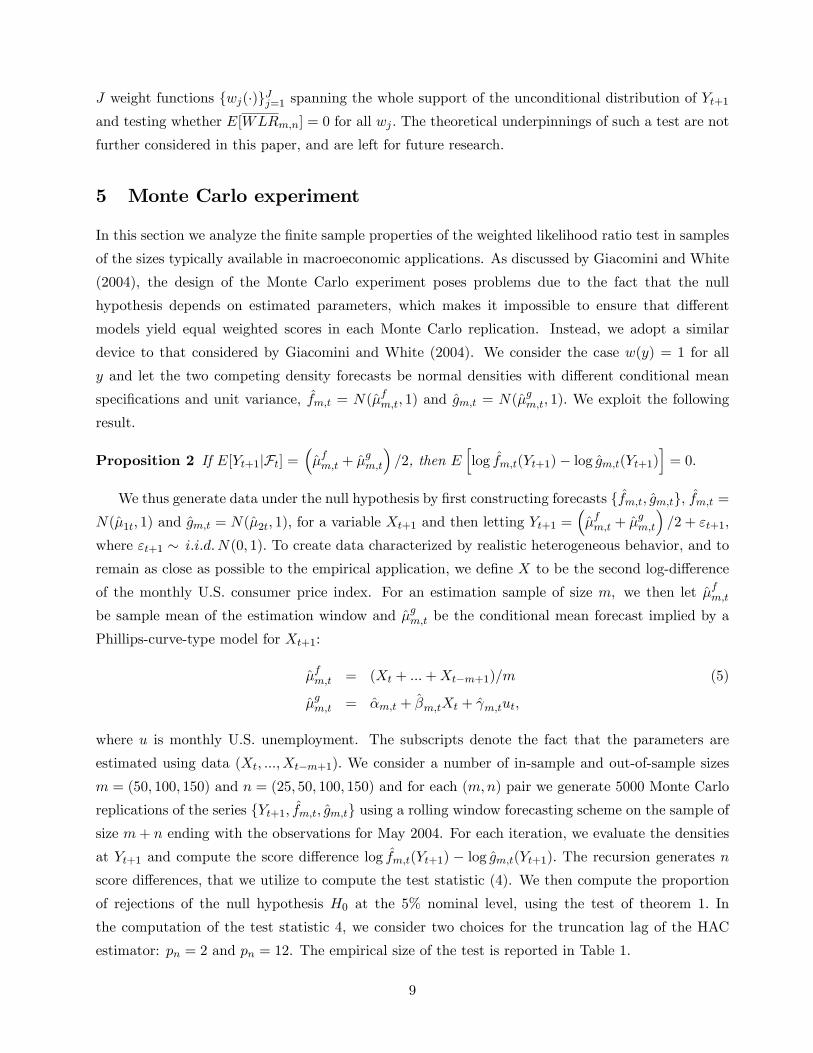
5 Monte Carlo experiment

In this section we analyze the �nite sample properties of the weighted likelihood ratio test in samples

of the sizes typically available in macroeconomic applications. As discussed by Giacomini and White

(2004), the design of the Monte Carlo experiment poses problems due to the fact that the null

hypothesis depends on estimated parameters, which makes it impossible to ensure that di¤erent

models yield equal weighted scores in each Monte Carlo replication. Instead, we adopt a similar

device to that considered by Giacomini and White (2004). We consider the case w(y) = 1 for all

y and let the two competing density forecasts be normal densities with di¤erent conditional mean

speci�cations and unit variance, fm;t = N(�fm;t; 1) and gm;t = N(�gm;t; 1): We exploit the following

result.

Proposition 2 If E[Yt+1jFt] =��fm;t + �

gm;t

�=2, then E

hlog fm;t(Yt+1)� log gm;t(Yt+1)

i= 0:

We thus generate data under the null hypothesis by �rst constructing forecasts ffm;t; gm;tg; fm;t =N(�1t; 1) and gm;t = N(�2t; 1); for a variable Xt+1 and then letting Yt+1 =

��fm;t + �

gm;t

�=2 + "t+1;

where "t+1 � i:i:d:N(0; 1): To create data characterized by realistic heterogeneous behavior, and to

remain as close as possible to the empirical application, we de�ne X to be the second log-di¤erence

of the monthly U.S. consumer price index. For an estimation sample of size m; we then let �fm;tbe sample mean of the estimation window and �gm;t be the conditional mean forecast implied by a

Phillips-curve-type model for Xt+1:

�fm;t = (Xt + :::+Xt�m+1)=m (5)

�gm;t = �m;t + �m;tXt + m;tut;

where u is monthly U.S. unemployment. The subscripts denote the fact that the parameters are

estimated using data (Xt; :::; Xt�m+1): We consider a number of in-sample and out-of-sample sizes

m = (50; 100; 150) and n = (25; 50; 100; 150) and for each (m;n) pair we generate 5000 Monte Carlo

replications of the series fYt+1; fm;t; gm;tg using a rolling window forecasting scheme on the sample ofsize m+ n ending with the observations for May 2004. For each iteration, we evaluate the densities

at Yt+1 and compute the score di¤erence log fm;t(Yt+1) � log gm;t(Yt+1): The recursion generates nscore di¤erences, that we utilize to compute the test statistic (4). We then compute the proportion

of rejections of the null hypothesis H0 at the 5% nominal level, using the test of theorem 1: In

the computation of the test statistic 4, we consider two choices for the truncation lag of the HAC

estimator: pn = 2 and pn = 12. The empirical size of the test is reported in Table 1.

9

[TABLE 1 HERE]

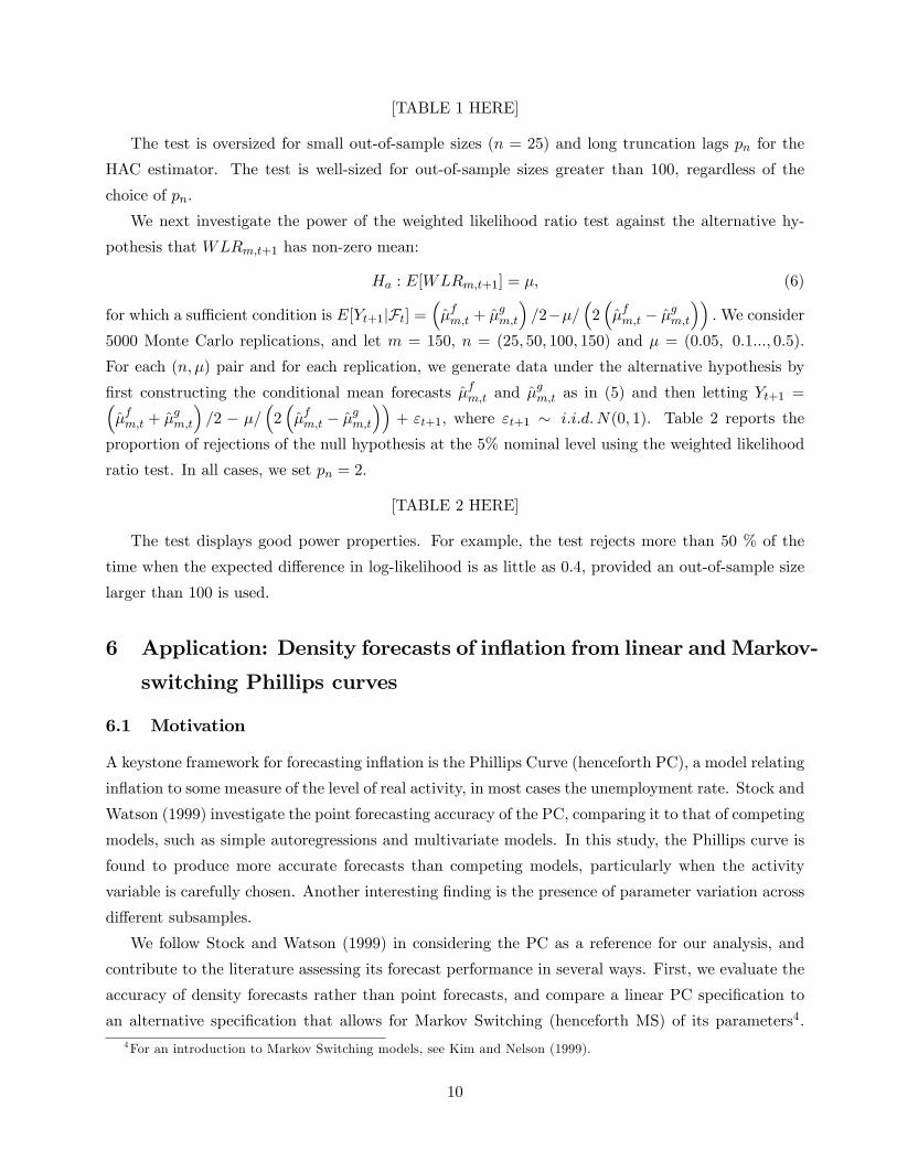
The test is oversized for small out-of-sample sizes (n = 25) and long truncation lags pn for the

HAC estimator. The test is well-sized for out-of-sample sizes greater than 100, regardless of the

choice of pn:

We next investigate the power of the weighted likelihood ratio test against the alternative hy-

pothesis that WLRm;t+1 has non-zero mean:

Ha : E[WLRm;t+1] = �; (6)

for which a su¢ cient condition is E[Yt+1jFt] =��fm;t + �

gm;t

�=2��=

�2��fm;t � �

gm;t

��:We consider

5000 Monte Carlo replications, and let m = 150; n = (25; 50; 100; 150) and � = (0:05; 0:1:::; 0:5):

For each (n; �) pair and for each replication, we generate data under the alternative hypothesis by

�rst constructing the conditional mean forecasts �fm;t and �gm;t as in (5) and then letting Yt+1 =�

�fm;t + �gm;t

�=2 � �=

�2��fm;t � �

gm;t

��+ "t+1; where "t+1 � i:i:d:N(0; 1). Table 2 reports the

proportion of rejections of the null hypothesis at the 5% nominal level using the weighted likelihood

ratio test. In all cases, we set pn = 2.

[TABLE 2 HERE]

The test displays good power properties. For example, the test rejects more than 50 % of the

time when the expected di¤erence in log-likelihood is as little as 0.4, provided an out-of-sample size

larger than 100 is used.

6 Application: Density forecasts of in�ation from linear andMarkov-

switching Phillips curves

6.1 Motivation

A keystone framework for forecasting in�ation is the Phillips Curve (henceforth PC), a model relating

in�ation to some measure of the level of real activity, in most cases the unemployment rate. Stock and

Watson (1999) investigate the point forecasting accuracy of the PC, comparing it to that of competing

models, such as simple autoregressions and multivariate models. In this study, the Phillips curve is

found to produce more accurate forecasts than competing models, particularly when the activity

variable is carefully chosen. Another interesting �nding is the presence of parameter variation across

di¤erent subsamples.

We follow Stock and Watson (1999) in considering the PC as a reference for our analysis, and

contribute to the literature assessing its forecast performance in several ways. First, we evaluate the

accuracy of density forecasts rather than point forecasts, and compare a linear PC speci�cation to

an alternative speci�cation that allows for Markov Switching (henceforth MS) of its parameters4.4For an introduction to Markov Switching models, see Kim and Nelson (1999).

10

We choose the MS model as a credible competitor to the linear PC model both because the MS

mechanism allows for parameter variation over the business cycle and because the predictive distri-

bution generated by the MS model is non-Gaussian, which is of potential interest when comparing

density forecast performance. Our second contribution is the evaluation of the impact on forecast

performance of using di¤erent estimation techniques when producing the forecasts. In particular,

we consider estimating both the linear and the MS model by either classical or Bayesian methods.

Note that a formal comparison of these forecast methods could not be conducted using previously

available techniques, since they do not easily accommodate nested model comparisons and Bayesian

estimation. This application thus gives a �avor of the generality of the forecasting comparisons that

can be performed using our testing framework.

6.2 Linear and Markov-switching Phillips curve

Following Stock and Watson (1999), our linear model is a PC model in which changes of in�ation

depend on their lags and on lags of the unemployment rate:

��t = �+ �(L)��t + (L)ut + � � "t (7)

�(L) =

p�Xi=1

�iLi; (L) =

puXi=1

iLi; "t v N:i:d:(0; 1)

�t = 100� ln(CPIt=CPIt�12);

where CPIt is the consumer price index and ut is the unemployment rate. This speci�cation is

consistent with the "natural rate hypothesis", since the natural rate of unemployment (NAIRU) is

u� = � � (1) : Note that we implicitly assume that��t and ut do not have a unit root

5. We started from

a general model with maximum lag orders p� and pu set to 12. Standard model reduction techniques6

allowed us to constrain the starting model and settle for a more parsimonious speci�cation:

��t = �+ �1��t�1 + �12��t�2 + �12��t�12 + ut�1 + � � "t (8)

� X 0t�1� + � � "t (9)

This speci�cation seems to be appropriate also across di¤erent non-overlapping 15 year subperiods

(1959:01-1973:12, 1974:01-1988:12, 1989:01-2004:07) and generates non-correlated residuals7.

In order to allow for potentially non-Gaussian density forecasts, we consider Markov Switching

models as competitors to the linear model (8). We do this by using the parameterization (8) and

assuming that some of the parameters vary depending on the value of an unobserved discrete variable

5We have run the usual ADF tests to check for the presence of a unit root in �t and ut. The testing results (available

on request) con�rm that �t has a unit root, whereas ut does not. These results hold across subperiods.6We estimated the model over the entire sample and then used the general-to-speci�c approach to eliminate all

insigni�cant regressors, testing the restrictions being imposed.7Note the inclusion of the 12th lag of the dependend variable: the signi�cance of this lag is robust across subperiods.

11

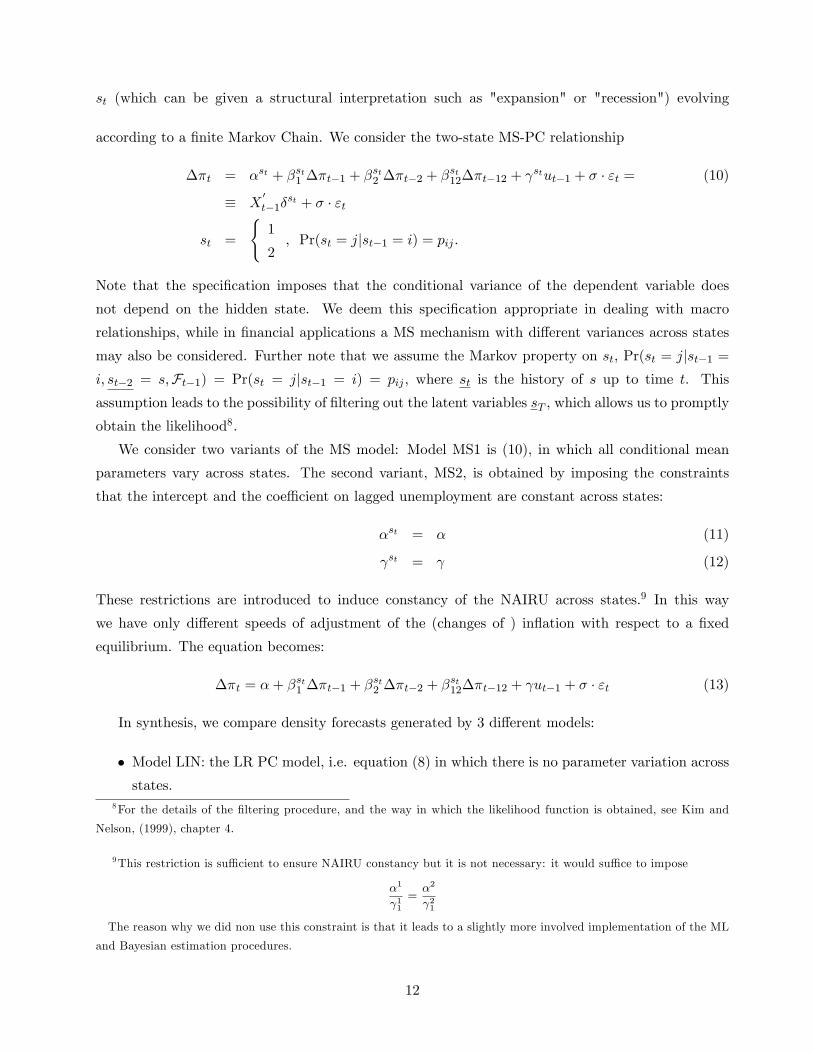
st (which can be given a structural interpretation such as "expansion" or "recession") evolving

according to a �nite Markov Chain. We consider the two-state MS-PC relationship

��t = �st + �st1 ��t�1 + �st2 ��t�2 + �

st12��t�12 +

stut�1 + � � "t = (10)

� X0t�1�

st + � � "t

st =

(1

2; Pr(st = jjst�1 = i) = pij :

Note that the speci�cation imposes that the conditional variance of the dependent variable does

not depend on the hidden state. We deem this speci�cation appropriate in dealing with macro

relationships, while in �nancial applications a MS mechanism with di¤erent variances across states

may also be considered. Further note that we assume the Markov property on st, Pr(st = jjst�1 =i; st�2 = s;Ft�1) = Pr(st = jjst�1 = i) = pij , where st is the history of s up to time t. This

assumption leads to the possibility of �ltering out the latent variables sT , which allows us to promptly

obtain the likelihood8.

We consider two variants of the MS model: Model MS1 is (10), in which all conditional mean

parameters vary across states. The second variant, MS2, is obtained by imposing the constraints

that the intercept and the coe¢ cient on lagged unemployment are constant across states:

�st = � (11)

st = (12)

These restrictions are introduced to induce constancy of the NAIRU across states.9 In this way

we have only di¤erent speeds of adjustment of the (changes of ) in�ation with respect to a �xed

equilibrium. The equation becomes:

��t = �+ �st1 ��t�1 + �

st2 ��t�2 + �

st12��t�12 + ut�1 + � � "t (13)

In synthesis, we compare density forecasts generated by 3 di¤erent models:

� Model LIN: the LR PC model, i.e. equation (8) in which there is no parameter variation acrossstates.

8For the details of the �ltering procedure, and the way in which the likelihood function is obtained, see Kim and

Nelson, (1999), chapter 4.

9This restriction is su¢ cient to ensure NAIRU constancy but it is not necessary: it would su¢ ce to impose

�1

11=�2

21

The reason why we did non use this constraint is that it leads to a slightly more involved implementation of the ML

and Bayesian estimation procedures.

12

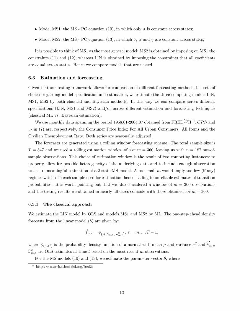
� Model MS1: the MS - PC equation (10), in which only � is constant across states;

� Model MS2: the MS - PC equation (13), in which �, � and are constant across states;

It is possible to think of MS1 as the most general model; MS2 is obtained by imposing on MS1 the

constraints (11) and (12), whereas LIN is obtained by imposing the constraints that all coe¢ cients

are equal across states. Hence we compare models that are nested.

6.3 Estimation and forecasting

Given that our testing framework allows for comparison of di¤erent forecasting methods, i.e. sets of

choices regarding model speci�cation and estimation, we estimate the three competing models LIN,

MS1, MS2 by both classical and Bayesian methods. In this way we can compare across di¤erent

speci�cations (LIN, MS1 and MS2) and/or across di¤erent estimation and forecasting techniques

(classical ML vs. Bayesian estimation).

We use monthly data spanning the period 1958:01-2004:07 obtained from FRED R II10. CPIt andut in (7) are, respectively, the Consumer Price Index For All Urban Consumers: All Items and the

Civilian Unemployment Rate. Both series are seasonally adjusted.

The forecasts are generated using a rolling window forecasting scheme. The total sample size is

T = 547 and we used a rolling estimation window of size m = 360, leaving us with n = 187 out-of-

sample observations. This choice of estimation window is the result of two competing instances: to

properly allow for possible heterogeneity of the underlying data and to include enough observation

to ensure meaningful estimation of a 2-state MS model. A too small m would imply too few (if any)

regime switches in each sample used for estimation, hence leading to unreliable estimates of transition

probabilities. It is worth pointing out that we also considered a window of m = 300 observations

and the testing results we obtained in nearly all cases coincide with those obtained for m = 360.

6.3.1 The classical approach

We estimate the LIN model by OLS and models MS1 and MS2 by ML. The one-step-ahead density

forecasts from the linear model (8) are given by:

fm;t = �(X0tb�m;t ; b�2m;t); t = m; :::; T � 1;

where �(�;�2) is the probability density function of a normal with mean � and variance �2 and b�0m;t;b�2m;t are OLS estimates at time t based on the most recent m observations.

For the MS models (10) and (13), we estimate the parameter vector �, where

10 http://research.stlouisfed.org/fred2/.

13

� =��1; �11; �

12; �

112,

1; �2; �21; �22; �

212;

2; �; p11; p21�0; (MS1)

� =��; �11; �

12; �

112; ; �

21; �

22; �

212; �; p11; p21

�0(MS2),

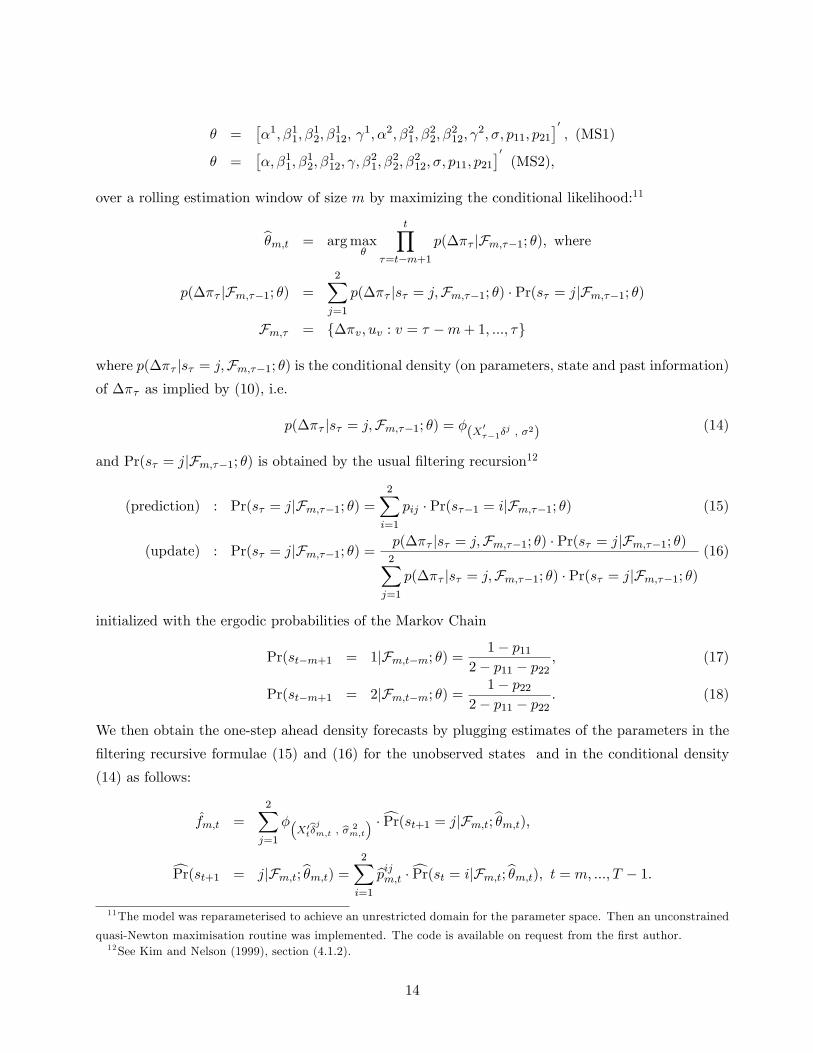
over a rolling estimation window of size m by maximizing the conditional likelihood:11

b�m;t = argmax�

tY�=t�m+1

p(��� jFm;��1; �); where

p(��� jFm;��1; �) =

2Xj=1

p(��� js� = j;Fm;��1; �) � Pr(s� = jjFm;��1; �)

Fm;� = f��v; uv : v = � �m+ 1; :::; �g

where p(��� js� = j;Fm;��1; �) is the conditional density (on parameters, state and past information)of ��� as implied by (10), i.e.

p(��� js� = j;Fm;��1; �) = �(X0��1�

j ; �2) (14)

and Pr(s� = jjFm;��1; �) is obtained by the usual �ltering recursion12

(prediction) : Pr(s� = jjFm;��1; �) =2Xi=1

pij � Pr(s��1 = ijFm;��1; �) (15)

(update) : Pr(s� = jjFm;��1; �) =p(��� js� = j;Fm;��1; �) � Pr(s� = jjFm;��1; �)2Xj=1

p(��� js� = j;Fm;��1; �) � Pr(s� = jjFm;��1; �)(16)

initialized with the ergodic probabilities of the Markov Chain

Pr(st�m+1 = 1jFm;t�m; �) =1� p11

2� p11 � p22; (17)

Pr(st�m+1 = 2jFm;t�m; �) =1� p22

2� p11 � p22: (18)

We then obtain the one-step ahead density forecasts by plugging estimates of the parameters in the

�ltering recursive formulae (15) and (16) for the unobserved states and in the conditional density

(14) as follows:

fm;t =2Xj=1

��X0tb�jm;t ; b� 2

m;t

� �cPr(st+1 = jjFm;t;b�m;t);cPr(st+1 = jjFm;t;b�m;t) = 2X

i=1

bpijm;t �cPr(st = ijFm;t;b�m;t); t = m; :::; T � 1:11The model was reparameterised to achieve an unrestricted domain for the parameter space. Then an unconstrained

quasi-Newton maximisation routine was implemented. The code is available on request from the �rst author.12See Kim and Nelson (1999), section (4.1.2).

14

6.3.2 The Bayesian approach

An alternative approach is to use simulation-based Bayesian inferential techniques. We start from

weakly informative priors (i.e., loose but proper priors), we combine them with the likelihood and

obtain the joint posterior. We Use Markov Chain Monte Carlo techniques to perform posterior

simulation. For the details, see Geweke (1999) and Kim and Nelson (1999, Ch. 7).

Bayesian estimation of the LIN model In the LIN model we give � and h = ��2 conditionally

conjugate priors:

� v N(��;H�1

� ) (19)

s � h v �2� (20)

i.e. priors that generate conditional posteriors for � and h that take the same analytical form as

the priors. These priors depend on 4 hyperparameters: ��and H� are respectively the prior mean

and precision of the � vector; s and � de�ne a Gamma prior for h = 1�2

13.Hence, the posterior

distribution of � = [�0; h]

0can be simulated by a simple 2-step Gibbs sampling algorithm, using the

posterior distribution of � conditional on h and the posterior distribution of h conditional on �.

Given a sample of draws from the joint posterior distribution

�(i) v p(�jFm;t); i = 1; 2; :::;M (21)

we can obtain density forecasts in two di¤erent ways:

� The Fully Bayesian (FB) way, i.e. by integrating unknown parameters out

fm;t =1

M

MXi=1

p(Yt+1jFm;t; �(i))d!Zp(Yt+1jFm;t; �)p(�jFm;t)d� (22)

� The "Empirical Bayes" (EB or plug-in) way, i.e. by plugging a parameter con�guration b�:fm;t = p(Yt+1jFm;t;b�) (23)

where b� is taken to synthesize the whole posterior distribution p(�jFm;t), i.e. it could be anestimate of the posterior mode, mean or median.

One could argue that the FB way is conceptually superior to the alternative, in that it takes into

account the role of parameter uncertainty, whereas the EB way ignores the uncertainty around point

estimates, as the density forecasts obtained using the ML approach do. Nonetheless, we chose to also

report EB density forecast evaluations in order to compare Bayesian with non-Bayesian approaches.13The choice of the hyperparameters s and � can be �exibly used to calibrate the prior mean and prior variance of

h = 1�2since

E(h) =�

s; V (h) =

2�

s2:

Note that non-dogmatic settings for these hyperparameters lead to a conditional posterior for h which is dominated by

data evidence.

15

Bayesian estimation of MS models Bayesian inference in MS models is complicated by the fact

that these models involve a latent variable. For the details, see Kim and Nelson (1999, chapter 9)

and Geweke and Amisano (2004). We use priors (19) and (20) on the regression coe¢ cients

�=h�01; �

02

i0(24)

and on h = ��2. In the partition (24) for �; �1 are the �rst order parameters that are �xed across

regimes and �2 are the �rst order parameters that vary across states. For example, in MS1 we

have �1 = 0 and �2 = [�1; �11; �12; �

112;

1; �2; �21; �22; �

212;

2]0; while in MS2 �1 = [�; ]

0and �2 =

[�11; �12; �

112; �

21; �

22; �

212]

0:We collect the transition probabilities in the 2�2matrix P and impose a Beta

(Dirichlet prior): (p11; p12) v Dir(r11; r12) and (p22; p22) v Dir(r21; r22). An easy Bayesian MCMCanalysis of the MS models is based on a conceptually simple Gibbs sampling-data augmentation

algorithm in which latent variables are sequentially simulated like a block of parameters. The

algorithm (for details, see chapter 9 of Kim and Nelson, 1999, or Geweke and Amisano, 2004) is

initialized by drawing �, h; P from their prior distributions, and then is based on the cyclical repetition

of the following steps: (1) draw st;m = fs� ; � = t�m+ 1; :::; tg from its conditional distribution

conditional on �; h; P (data-augmentation step in which latent variables are simulated); (2) draw

� from its conditional distribution conditional on h and on st;m; (3) draw h from its conditional

distribution conditional on � and on st;m; (4) draw P from its conditional distribution conditional

on st;m: The resulting Markov Chain converges in distribution to the joint posterior distribution of

�; h; P; st;m . The models MS1 and MS2 are simulated in the same way.

To produce density forecasts, we use a FB method:

fm;t =1

M

MXi=1

2Xj=1

��X0t�j(i);�2(i)

� � p(st+1 = jjFm;t; �(i)) (25)

d!2Xj=1

Zp(��t+1jFm;t; st+1 = j; �) � p(st+1 = jjFm;t; �) � p(�jFm;t)d� =

= p(��t+1jFm;t) (26)

which is based on the marginalization with respect to the unknown parameters and the unknown

state variables.

Alternatively, we also consider an EB method

fm;t =2Xj=1

p(��t+1jst+1 = j;Ft;b�) � p(st+1 = jjFt;b�) (27)

in which b� is a synthetic value taken from the posterior density of �. In this case parameter uncertaintyis ignored whereas uncertainty about the latent variables st+1;m+1is properly accounted for through

marginalization.

16

6.4 Discussion of the results

We performed ML and Bayesian estimation of the three models LIN, MS1 and MS2 in (8), (10) and

(13). Estimation was carried out by Matlab14. With reference to (19) and (20), in model LIN we use

as hyperparameters

��=

266666664

0:1

0:0

0:0

0:0

�0:04

377777775; H� =

�1

0:2

�2� I5; s = 0:3, � = 3: (28)

For the MS1 and MS2 models we used the same hyperparameters s = 0:3; � = 3 as in the LIN model;

for the regression coe¢ cients we used the following prior hyperparameters

MS1 : ��=

"1

1

#

266666664

0:1

0:0

0:0

0:0

�0:04

377777775; H� =

�1

0:2

�2� I10 (29)

MS2 : ��=

266666664

0:1

�0:4"1

1

#

26640:0

0:0

0:0

3775

377777775; H� =

�1

0:2

�2� I8 (30)

whereas for the Dirichlet prior for the rows of P we used

R=

"8 2

2 8

#: (31)

All the prior distributions are proper, quite loose, symmetric across unobserved states, and the prior

on P imparts relevant persistence on the unobservable states.

In terms of point parameter estimates, we did not �nd many di¤erences between Bayesian and

ML estimates, once the label switching problem of the MS models is properly accounted for (see for

details, Geweke and Amisano, 2004). For this reason we decided to report only point ML estimates

of the parameters in Figures 2 to 4.14The codes can be requested to the �rst author. They require the availability of the Matlab toolboxes Optimization

and Statistics. ML is carried out by reparameterizing the model in a way that parameters are de�ned on an

unrestricted domain and then minus the loglikelihood is minimized using the Matlab function fminunc.Also Bayesian

inference is carried out by using Matlab routines based on the availability of the same toolboxes. The �ltering code

used for �ltering out the latent variables was coded in Fortran and linked up as a dll in Matlab (MMfilter.dll).

17

[FIGURE 2 HERE]

Figure 2 shows the estimation results of the LIN model. Note that individual parameters seem to

vary quite a lot, but the estimated NAIRU (bottom left) \NAIRU = �c�0c 1 and the estimated "speed

of adjustment" (SP, degree of mean reversion, bottom center) bsp = b�1+b�2+b�12�1; tend to be morestable. In particular, the estimated NAIRU is quite high, hovering around 6%, with only a slight

drop in the second half of the 1990s. This is in contrast to the commonly held belief15 that the PC,

and the NAIRU in particular, changed radically in the prolonged expansion that took place in the

1990s. The estimated speed of adjustment, measuring the degree of mean reversion, can be viewed

as indicating how easy it is to forecast changes of in�ation in the short term: when SP becomes more

negative, as from 1999 onwards, it becomes harder to forecast ��t, at least in the short term.

[FIGURE 3 HERE]

In Figure 3 we report ML parameter estimates of the conditional mean parameters � and the

precision parameter h = ��2 for the MS1 model. Our main remarks are: (1) the MS model parameter

estimates are more stable than their LIN model counterpart; (2) the interpretation of state 1 being

"expansion" and state 2 being "recession" is coherent with the �ndings that the NAIRU in state 2 is

higher than in state 1 and that the persistence of state 1, p11, is higher than the persistence of state

2, p22 (consistent with recessions having shorter duration than expansions); (3) in state 2 NAIRU is

almost constant whereas in state 1 it drops sharply in the second half of the 1990s.

Figure 4 reports results of the estimation of MS2 model.

[FIGURE 4 HERE]

Note that: (1) it is problematic to identify states: they have the same persistence and they are

associated with the same NAIRU. State 1 is associated with higher speed of adjustment; (2) NAIRU

estimates are in the same range as for the LIN model, and they have the same time evolution; (3) h

has the same time evolution as in the LIN and MS1 cases.

Turning to the evaluation of the density forecast performance of the competing models, we con-

sider the sequence of one-step-ahead density forecasts implied by the three models, using the ML,

FB and EB estimation approaches. We conduct pairwise WLR tests and report the results in Ta-

bles 3A-3C. In the computation of the test statistic (4) we use a Newey-West estimator of �2n with

bandwidth � = 6: Di¤erent values for � have no impact on the results.

Table 3A reports the unweighted (!0) case.

[TABLE 3A HERE]

15See for instance the results presented in Staiger et al. (2001), where the NAIRU is found to have dropped of more

than 1% in the 1995-2000 period.

18

Table 3A shows that LIN is signi�cantly worse than either MS1 or MS2. This �nding is robust to

the estimation method: using both the ML and the FB approach, LIN fares signi�cantly worse than

both competitors. Using the EB approach, conclusions are not that clear-cut, since the di¤erences

are not signi�cant. As for comparison between MS1 and MS2, they are not signi�cantly di¤erent for

the EB case, but MS1 outperforms MS2 in both ML and FB estimation case. In general, we conclude

that the winner seems to be the MS1 model and that the best performance is achieved by using ML

estimation.

Table 3B shows results for the Center-weighted case (!1).

[TABLE 3B HERE]

The conclusions are nearly the same as in the previous case: MS1 dominates MS2 and LIN, both

in the classical estimation framework (ML) and in a Bayesian context (FB). Using the EB approach

generally yields insigni�cant di¤erences.

For the Tails-weighted case (!2) the results are in Table 3C.

[TABLE 3C HERE]

Here we have partially di¤erent results: in fact, using the ML results, LIN is signi�cantly worse

than MS2 only, but the MS1-MS2 di¤erence is not signi�cant. These conclusions are not robust to

estimation and forecasting method: FB di¤erences are not signi�cant at all while EB shows dominance

of the LIN model. We believe that these �ndings can be due to the fact that the weighting scheme

assigns negligible weights to observations near the sample mean of the dependent variable in�ation, in

this way blurring the di¤erences among models. This interpretation is con�rmed by visual inspection

of the sample weights (see Figure 5, bottom center), in which it is evident that nearly half of the

observations are assigned weights close to zero.

[FIGURE 5 HERE]

For the Right Tail-weighted case (!3) the results are contained in Table 3D.

[TABLE 3D HERE]

This weighting scheme can be viewed as assigning importance to good density forecast properties

when in�ation is rising fast. The conclusions in this case are very similar to the unweighted case:

LIN is signi�cantly outperformed by MS1 and MS2 and this is robust to the estimation method (ML

and FB). MS1 outperforms MS2, robust with respect to estimation method (ML, FB). The MS1

appears to be the best model and the best way to obtain density forecasts is to use ML estimation.

For the Left Tail weighted case (!4) the results are contained in Table 3E.

[TABLE 3E HERE]

19

Also in this case, LIN is signi�cantly worse than MS1 and MS2, both with the ML and FB

approaches and the evidence for EB estimation is not signi�cant. Note also that in this case MS1 is

signi�cantly better than MS2 only in the FB approach.

Summing up the whole evidence, it appears that the Markov-switching MS1 model outperforms

both alternatives. This happens in the unweighted case and in most of the weighted cases. Only in

the Tails weighted (!2) case, we have a less clear picture, but this is likely to be due to excessive

penalty attributed to the values near the center of the distribution of the dependent variable. We

also generally conclude that maximum likelihood estimation yields better forecasts than Bayesian

estimation.

6.5 Comparison with predictive posterior odds ratios

As a �nal piece of evidence regarding the relative performance of the three models, we consider

Bayesian model comparison based on posterior odds ratios (POR):

PORi;j =p(MijY )p(Mj jY )

=p(Mi)

p(Mj)

p(Y jMi)

p(Y jMj)(32)

p(Y jMi)

p(Y jMj)= Bayes factor =

p(Y1jY0;Mi)

p(Y1jY0;Mj)� p(Y0jMi)

p(Y0jMj)(33)

where Y0 contains all data up to observation m and Y1 contains the data after m. A PORi;j greater

than one indicates that model i outperforms model j: The predictive Bayes factor PBF = p(Y1jY0;Mi)p(Y1jY0;Mj)

is the ratio of the predictive densities of Y1 based on the two competing models, which can be

computed by recursively simulating the posterior distribution of the parameters:

p(Y1jY0;Mj) =TY

t=m+1

p(YtjYt�1;Mj) (34)

p(YtjYt�1;Mj) =1

M

MXi=1

p(YtjYt�1;Mj ; �(i))

d! p(YtjYt�1;Mj) (35)

�(i) v p(�jYt�1;Mj): (36)

In our application, the PBF from LIN versus MS1 and MS2 are respectively 2.73E-07 and 7.55E-

06, indicating that the linear model is clearly outperformed by the Markov-switching models. The

PBF for MS1 versus MS2 is 27.6, suggesting that MS1 is the clear winner. The conclusion from

Bayesian predictive model comparison is thus in concordance with that from the WLR tests. We

should however point out that, unlike the WLR testing procedure, the comparison based on the

predictive Bayes factor does not allow for time variation in the data generating process.

20

7 Conclusion

We introduced a weighted likelihood ratio test for comparing the out-of-sample performance of com-

peting density forecasts of a variable. We proposed measuring the performance of the density forecasts

by scoring rules, which are loss functions de�ned over the probability forecast and the outcome of the

variable. In particular, we restricted attention to the logarithmic scoring rule, and suggested ranking

the forecasts according to the relative magnitude of a weighted average of the scores measured over

the available sample. We showed that the use of weights introduces �exibility by allowing the user to

isolate the performance of competing density forecasts in di¤erent regions of the unconditional dis-

tribution of the variable of interest. Loosely speaking, the test can help distinguish, for example, the

relative forecast performance in �normal�days from that in days when the variable takes on �extreme�

values. The special case of equal weights is also of interest, since in this case our test is related to

Vuong�s (1989) likelihood ratio test for non-nested hypotheses. Unlike Vuong�s (1989) test, however

our test is performed out-of-sample rather than in-sample, it is valid for both nested and non-nested

forecast models, and it considers time series rather than i.i.d. data.

Our test can be applied to time-series data characterized by a considerable amount of heterogene-

ity and dependence (including possible structural changes) and it is valid under general conditions.

In particular, the underlying forecast models can be either nested or non-nested and the forecasts

can be produced by utilizing parametric as well as semi-parametric, non-parametric or Bayesian es-

timation procedures. The only requirement that we impose is that the forecasts are based on a �nite

estimation window, as in Giacomini and White (2004).

We applied our test to a comparison of density forecasts produced by di¤erent versions of a

univariate Phillips Curve, based on monthly US data over the last 40 years: a linear regression, a

2-state Markov Switching regression and a 2-state Markov Switching regression in which the natural

rate of unemployment was constrained to be equal across states. Note that these models imply

di¤erent shapes for the density of in�ation: a normal density for the linear model and a mixture

of normals for the Markov-switching models. In the comparison we also considered versions of each

model estimated by maximum likelihood or by Bayesian techniques.

Our general conclusion was that density forecasts from the MS1 model outperformed all alter-

natives. This happened in the unweighted case and in most of the weighted cases. Only in the

Tails-weighted case, the three models could not be discriminated, but this is likely to be due to

excessive penalization of the values near the center of the distribution of the dependent variable.

We also found that maximum likelihood estimation seemed to yield superior forecasts than Bayesian

alternatives.

21

8 Proofs

Proof of Theorem 1. We show that assumptions (i)-(iii) of Theorem 6 of Giacomini and White

(2004) (which we denote by GW1-GW3) are satis�ed by letting Wt � Zt and �Lm;t+1 �WLRm;t+1;from which (a) and (b) follow.

GW1 coincides with assumption (i).

GW2 imposes the existence of 2r moments ofWLRm;t+1 = w(Yt+1)(log fm;t(Yt+1)�log gm;t(Yt+1))for some r > 2: From assumption (ii), there exists a r0 > 2 such that Ej log fm;t(Yt+1)j2r

0<1. De�ne

r = r0

1+" , for some " > 0; so that r > 2: Since w(Ystt+1) � 0; and by applying Hölder�s inequality, we

have

Ejw(Y stt+1) log fm;t(Yt+1)j2r = E���w(Y stt+1)2rj log fm;t(Yt+1)j2r���

��Ew(Y stt+1)

2r 1+""

� "1+"(Ej log fm;t(Yt+1)j2r(1+"))

11+"

=�Ew(Y stt+1)

2r0"

� "1+"�Ej log fm;t(Yt+1)j2r

0� 11+"

<1;

where the last inequality holds since the �rst term is �nite because w (�) is bounded, and the secondterm is �nite by (ii). Similarly, Ejw(Y stt+1) log gm;t(Yt+1)j2r <1. By Minkowski�s inequality we thushave

EjWLRm;t+1j2r ���Ejw(Y stt+1) log fm;t(Yt+1)j2r

� 12r+�Ejw(Y stt+1) log gm;t(Yt+1)j2r

� 12r

�2r<1

Finally, GW3 coincides with assumption (iii).

Proof of Proposition 2. We have

E[log fm;t(Yt+1)� log gm;t(Yt+1)] =

EhE[log fm;t(Yt+1)� log gm;t(Yt+1)jFt]

i=

E

�E

��12

�Yt+1 � �fm;t

�2+1

2(Yt+1 � �gm;t)2jFt

��=

E

�1

2E

�2Yt+1

��fm;t � �

gm;t

����fm;t

�2+ (�gm;t)

2jFt��

=

Eh��fm;t � �

gm;t

��E[Yt+1jFt]�

��fm;t + �

gm;t

�=2�i

= 0;

where the last equality follows from the fact that E[Yt+1jFt] =��fm;t + �

gm;t

�=2:

22

References

[1] Andrews, D. W. K. (1991): �Heteroskedasticity and Autocorrelation Consistent Covariance

Matrix Estimation�, Econometrica, 59, 817-858.

[2] Artzner, P., Delbaen, F., Eber, J. M., Heath, D. (1997): �Thinking Coherently�, Risk, 10, 68-71.

[3] Berkowitz, J. (2001): �The Accuracy of Density Forecasts in Risk Management�, Journal of

Business and Economic Statistics, 19, 465-74.

[4] Christo¤ersen P. F., Diebold, F. X. (1997): �Optimal Prediction under Asymmetric Loss�,

Econometric Theory, 13, 808-817.

[5] Clements, M. P., Smith, J. (2000): �Evaluating the Forecast Densities of Linear and Non-

linear Models: Applications to Output Growth and Unemployment�, Journal of Forecasting, 19,

255-276.

[6] Corradi, V. and N. Swanson (2003): �Bootstrap Conditional Distribution Tests in the Presence

of Dynamic Misspeci�cation�, Journal of Econometrics, forthcoming

[7] Corradi, V. and N. Swanson (2004a): �Predictive Density and Conditional Con�dence Interval

Accuracy Tests�, Rutgers University working paper

[8] Corradi, V. and N. Swanson (2004b): �A Test for Comparing Multiple Misspeci�ed Conditional

Distributions�, Rutgers University working paper

[9] Diebold, F. X., Gunther, T. A., Tay, A. S. (1998): �Evaluating Density Forecasts with Applica-

tions to Financial Risk Management�, International Economic Review, 39, 863-883.

[10] Diebold, F. X., Lopez, J. A. (1996): �Forecast Evaluation and Combination�, in Handbook

of Statistics, Volume 14: Statistical Methods in Finance, G. S. Maddala, C. R. Rao (eds.).

Amsterdam: North-Holland, 241-268.

[11] Diebold, F. X., Tay, A.S., Wallis, K. F. (1999): �Evaluating Density Forecasts of In�ation: The

Survey of Professional Forecasters �, in R. Engle and H. White (eds.), Festschrift in Honour of

C.W.J. Granger, 76-90, Oxford University Press.

[12] Du¢ e, D., Pan, J. (1996): �An Overview of Value at Risk�, Journal of Derivatives, 4, 13-32.

[13] Geweke, J. and G. Amisano (2004):�Compound Markov Mixture Models with Applications in

Finance, mimeo.

[14] Giacomini, R. and H. White (2004): �Tests of conditional predictive ability�, mimeo, University

of California, Los Angeles and University of California, San Diego working paper.

23

[15] Hong, Y. (2000): �Evaluation of Out-of-Sample Density Forecasts with Applications to S&P

500 Stock Prices�, Cornell University manuscript.

[16] Hong, Y., White, H. (2000): �Asymptotic Distribution Theory for Nonparametric Entropy

Measures of Serial Dependence�, University of California, San Diego manuscript.

[17] Hong, Y. and H. Li (2003): �Out of Sample Performance of Spot Interest Rate Models�, Review

of Financial Studies, forthcoming

[18] Kim, C.J. and C. Nelson (1999): State Space Models with Regime Switching, MIT Press, Cam-

bridge, USA.

[19] Lopez, J. A. (2001): �Evaluating the Predictive Accuracy of Volatility Models�, Journal of

Forecasting, 20, 87-109.

[20] Newey, W. K., West, K. D. (1987): �A Simple, Positive Semide�nite, Heteroskedasticity and

Autocorrelation Consistent Covariance Matrix�, Econometrica, 55, 703-708.

[21] Patton, A. J. (2001): �Modelling Asymmetric Exchange Rate Dependence�, International Eco-

nomic Review, forthcoming.

[22] Soderlind, P., Svensson, L. (1997): �New Techniques to Extract Market Expectations from

Financial Instruments�, Journal of Monetary Economics, 40, 383-429.

[23] Steiger, D., J.H. Stock and M.W. Watson (2001): �Prices, wages and the U.S. NAIRU in the

1990s�, NBER working paper # 8320.

[24] Stock, J.H. and M.W. Watson (1999): �Forecasting In�ation�, Journal of Monetary Economics,

44, 293-335 .

[25] Tay, A. S., Wallis, K. F. (2000): �Density Forecasting: A Survey�, Journal of Forecasting, 19,

235-254.

[26] Vuong, Q. H. (1989): �Likelihood Ratio Tests for Model Selection and Non-nested Hypotheses�,

Econometrica, 57, 307-333.

[27] Weigend, A. S., Shi, S. (2000): �Predicting Daily Probability Distributions of S&P500 Returns�,

Journal of Forecasting, 19, 375-392.

[28] Weiss, A. A. (1996): �Estimating Time Series Models Using the Relevant Cost Function�,

Journal of Applied Econometrics, 11, 539-560.

[29] Winkler, R. L. (1967): �The Quanti�cation of Judgement: Some Methodological Suggestions�,

Journal of the American Statistical Association, 62, 1105-1120.

24

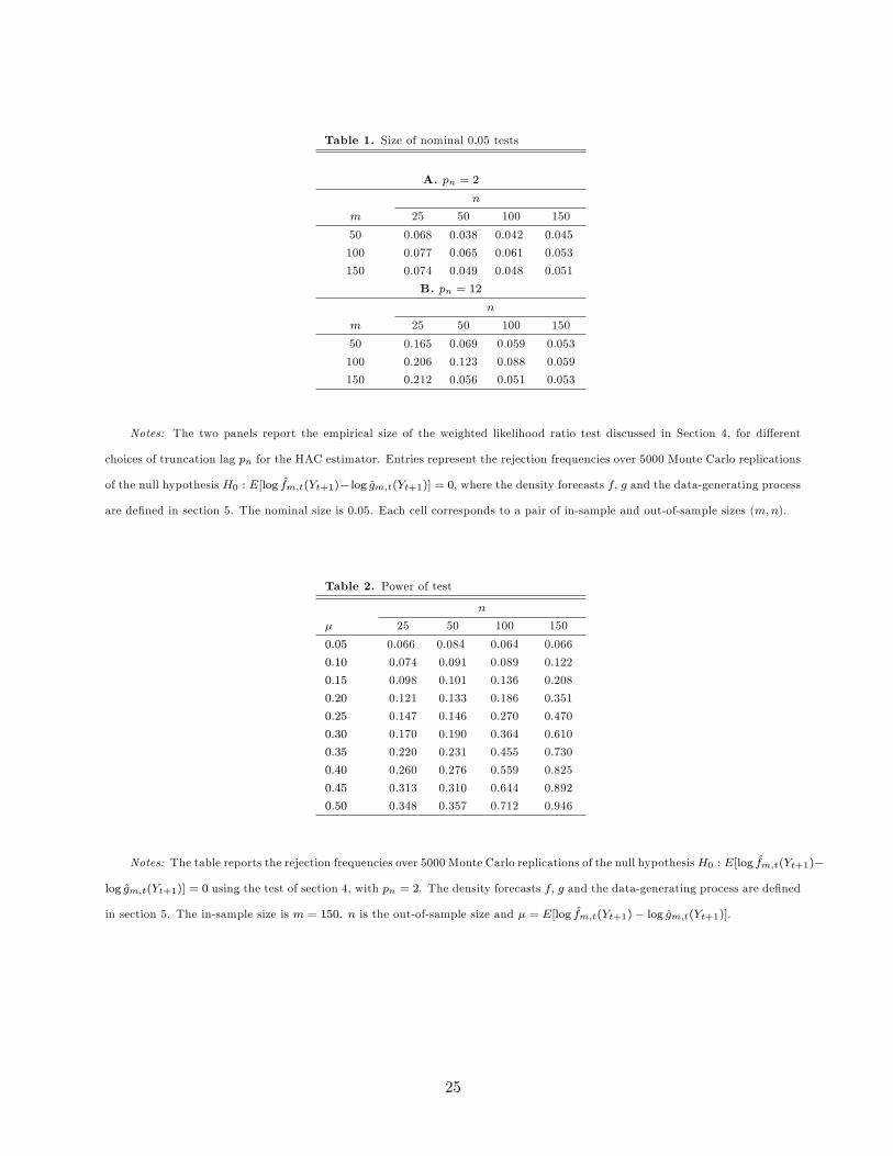
Table 1. Size of nominal 0.05 tests

A. pn = 2

n

m 25 50 100 150

50 0.068 0.038 0.042 0.045

100 0.077 0.065 0.061 0.053

150 0.074 0.049 0.048 0.051

B. pn = 12

n

m 25 50 100 150

50 0.165 0.069 0.059 0.053

100 0.206 0.123 0.088 0.059

150 0.212 0.056 0.051 0.053

Notes: The two panels report the empirical size of the weighted likelihood ratio test discussed in Section 4, for di¤erent

choices of truncation lag pn for the HAC estimator. Entries represent the rejection frequencies over 5000 Monte Carlo replications

of the null hypothesis H0 : E[log fm;t(Yt+1)� log gm;t(Yt+1)] = 0, where the density forecasts f; g and the data-generating process

are de�ned in section 5. The nominal size is 0.05. Each cell corresponds to a pair of in-sample and out-of-sample sizes (m;n).

Table 2. Power of test

n

� 25 50 100 150

0:05 0.066 0.084 0.064 0.066

0:10 0.074 0.091 0.089 0.122

0:15 0.098 0.101 0.136 0.208

0:20 0.121 0.133 0.186 0.351

0:25 0.147 0.146 0.270 0.470

0:30 0.170 0.190 0.364 0.610

0:35 0.220 0.231 0.455 0.730

0:40 0.260 0.276 0.559 0.825

0:45 0.313 0.310 0.644 0.892

0:50 0.348 0.357 0.712 0.946

Notes: The table reports the rejection frequencies over 5000 Monte Carlo replications of the null hypothesisH0 : E[log fm;t(Yt+1)�

log gm;t(Yt+1)] = 0 using the test of section 4, with pn = 2. The density forecasts f; g and the data-generating process are de�ned

in section 5. The in-sample size is m = 150. n is the out-of-sample size and � = E[log fm;t(Yt+1)� log gm;t(Yt+1)].

25

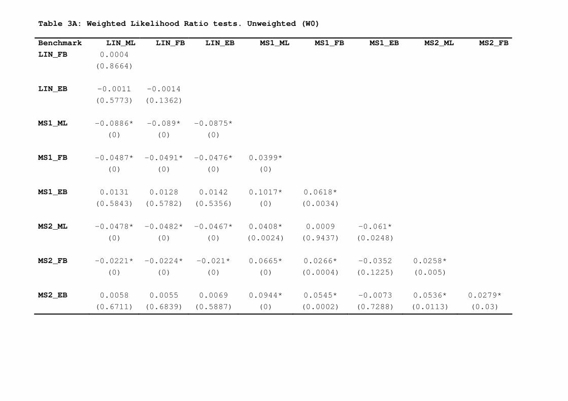
Table 3A: Weighted Likelihood Ratio tests. Unweighted (W0) Benchmark LIN_ML LIN_FB LIN_EB MS1_ML MS1_FB MS1_EB MS2_ML MS2_FB LIN_FB 0.0004 (0.8664) LIN_EB -0.0011 -0.0014 (0.5773) (0.1362) MS1_ML -0.0886* -0.089* -0.0875* (0) (0) (0) MS1_FB -0.0487* -0.0491* -0.0476* 0.0399* (0) (0) (0) (0) MS1_EB 0.0131 0.0128 0.0142 0.1017* 0.0618* (0.5843) (0.5782) (0.5356) (0) (0.0034) MS2_ML -0.0478* -0.0482* -0.0467* 0.0408* 0.0009 -0.061* (0) (0) (0) (0.0024) (0.9437) (0.0248) MS2_FB -0.0221* -0.0224* -0.021* 0.0665* 0.0266* -0.0352 0.0258* (0) (0) (0) (0) (0.0004) (0.1225) (0.005) MS2_EB 0.0058 0.0055 0.0069 0.0944* 0.0545* -0.0073 0.0536* 0.0279*

(0.6711) (0.6839) (0.5887) (0) (0.0002) (0.7288) (0.0113) (0.03)

Table 3B: Weighted Likelihood Ratio tests. Center (W1) Benchmark LIN_ML LIN_FB LIN_EB MS1_ML MS1_FB MS1_EB MS2_ML MS2_FB LIN_FB -0.0002 (0.6592) LIN_EB -0.0013* -0.0011* (0.0124) (0) MS1_ML -0.0338* -0.0336* -0.0325* (0) (0) (0) MS1_FB -0.0196* -0.0193* -0.0182* 0.0143* (0) (0) (0) (0) MS1_EB -0.0061 -0.0059 -0.0048 0.0277* 0.0134* (0.2764) (0.274) (0.3745) (0) (0.006) MS2_ML -0.0128* -0.0126* -0.0115* 0.021* 0.0067* -0.0067 (0) (0) (0) (0) (0.0236) (0.2573) MS2_FB -0.0093* -0.009* -0.0079* 0.0245* 0.0103* -0.0032 0.0036* (0) (0) (0) (0) (0) (0.5483) (0.0292) MS2_EB -0.0121* -0.0119* -0.0107* 0.0217* 0.0075* -0.006 0.0008 -0.0028 (0) (0) (0) (0) (0.0083) (0.224) (0.8232) (0.157)

Table 3C: Weighted Likelihood Ratio tests. Tails (W2) Benchmark LIN_ML LIN_FB LIN_EB MS1_ML MS1_FB MS1_EB MS2_ML MS2_FB LIN_FB 0.001 (0.5162) LIN_EB 0.0023* 0.0013 (0.0397) (0.1432) MS1_ML -0.0038 -0.0047 -0.0061 (0.7038) (0.6336) (0.5335) MS1_FB 0.0003 -0.0006 -0.002 0.0041 (0.9587) (0.913) (0.7299) (0.4697) MS1_EB 0.0285* 0.0275* 0.0262* 0.0323* 0.0282* (0.0193) (0.0175) (0.0226) (0.0274) (0.0125) MS2_ML -0.0156* -0.0166* -0.0179* -0.0118 -0.0159* -0.0441* (0.0406) (0.0235) (0.0218) (0.1823) (0.0329) (0.0042) MS2_FB 0.0012 0.0003 -0.0011 0.005 0.0009 -0.0273* 0.0168* (0.6556) (0.9244) (0.6629) (0.5153) (0.8296) (0.0203) (0.0091) MS2_EB 0.0361* 0.0352* 0.0338* 0.0399* 0.0358* 0.0076 0.0517* 0.0349* (0.0003) (0.0006) (0.0004) (0.0034) (0.0011) (0.4818) (0.001) (0.0004)

Table 3D: Weighted Likelihood Ratio tests. Right tail (W3) Benchmark LIN_ML LIN_FB LIN_EB MS1_ML MS1_FB MS1_EB MS2_ML MS2_FB LIN_FB -0.0002 (0.6592) LIN_EB -0.0013* -0.0011* (0.0124) (0) MS1_ML -0.0338* -0.0336* -0.0325* (0) (0) (0) MS1_FB -0.0196* -0.0193* -0.0182* 0.0143* (0) (0) (0) (0) MS1_EB -0.0061 -0.0059 -0.0048 0.0277* 0.0134* (0.2764) (0.274) (0.3745) (0) (0.006) MS2_ML -0.0128* -0.0126* -0.0115* 0.021* 0.0067* -0.0067 (0) (0) (0) (0) (0.0236) (0.2573) MS2_FB -0.0093* -0.009* -0.0079* 0.0245* 0.0103* -0.0032 0.0036* (0) (0) (0) (0) (0) (0.5483) (0.0292) MS2_EB -0.0121* -0.0119* -0.0107* 0.0217* 0.0075* -0.006 0.0008 -0.0028 (0) (0) (0) (0) (0.0083) (0.224) (0.8232) (0.157)

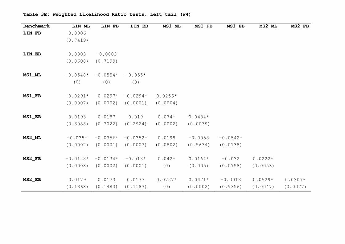
Table 3E: Weighted Likelihood Ratio tests. Left tail (W4) Benchmark LIN_ML LIN_FB LIN_EB MS1_ML MS1_FB MS1_EB MS2_ML MS2_FB LIN_FB 0.0006 (0.7419) LIN_EB 0.0003 -0.0003 (0.8608) (0.7199) MS1_ML -0.0548* -0.0554* -0.055* (0) (0) (0) MS1_FB -0.0291* -0.0297* -0.0294* 0.0256* (0.0007) (0.0002) (0.0001) (0.0004) MS1_EB 0.0193 0.0187 0.019 0.074* 0.0484* (0.3088) (0.3022) (0.2924) (0.0002) (0.0039) MS2_ML -0.035* -0.0356* -0.0352* 0.0198 -0.0058 -0.0542* (0.0002) (0.0001) (0.0003) (0.0802) (0.5634) (0.0138) MS2_FB -0.0128* -0.0134* -0.013* 0.042* 0.0164* -0.032 0.0222* (0.0008) (0.0002) (0.0001) (0) (0.005) (0.0758) (0.0053) MS2_EB 0.0179 0.0173 0.0177 0.0727* 0.0471* -0.0013 0.0529* 0.0307* (0.1368) (0.1483) (0.1187) (0) (0.0002) (0.9356) (0.0047) (0.0077)

Figure 1: weight functions (w1 = center of distribution, w2 = tails of distribution, w3 = right tail, w4 = left tail)

.0

.1

.2

.3

.4

.5

-6 -4 -2 0 2 4 6

Y

W1

0.0

0.2

0.4

0.6

0.8

1.0

-6 -4 -2 0 2 4 6

Y

W2

0.0

0.2

0.4

0.6

0.8

1.0

-6 -4 -2 0 2 4 6

Y

W3

0.0

0.2

0.4

0.6

0.8

1.0

-6 -4 -2 0 2 4 6

Y

W4

Figure 2: Linear Model (LIN) ML parameter estimates

.32

.33

.34

.35

.36

.37

.38

.39

.40

90 92 94 96 98 00 02

LIN_ML_A0

.22

.24

.26

.28

.30

.32

.34

.36

90 92 94 96 98 00 02

LIN_ML_B1

.04

.06

.08

.10

.12

.14

.16

.18

.20

90 92 94 96 98 00 02

LIN_ML_B2

-.43

-.42

-.41

-.40

-.39

-.38

-.37

90 92 94 96 98 00 02

LIN_ML_B12

-.062

-.061

-.060

-.059

-.058

-.057

-.056

-.055

-.054

-.053

90 92 94 96 98 00 02

LIN_ML_G1

.264

.268

.272

.276

.280

.284

.288

90 92 94 96 98 00 02

LIN_ML_SIG

6.08

6.12

6.16

6.20

6.24

6.28

6.32

6.36

90 92 94 96 98 00 02

LIN_ML_NAIRU

-1.04

-1.02

-1.00

-0.98

-0.96

-0.94

-0.92

90 92 94 96 98 00 02

LIN_ML_SP

Figure 3: Markov Switching MS1 model ML parameter estimates

0.0

0.5

1.0

1.5

2.0

2.5

3.0

90 92 94 96 98 00 02

MS1_ML_A0_1 MS1_ML_A0_2

-.3

-.2

-.1

.0

.1

.2

.3

.4

.5

90 92 94 96 98 00 02

MS1_ML_B1_1 MS1_ML_B1_2

-.12

-.08

-.04

.00

.04

.08

.12

.16

90 92 94 96 98 00 02

MS1_ML_B2_1 MS1_ML_B2_2

-.60

-.55

-.50

-.45

-.40

-.35

90 92 94 96 98 00 02

MS1_ML_B12_1 MS1_ML_B12_2

-.40

-.35

-.30

-.25

-.20

-.15

-.10

-.05

.00

90 92 94 96 98 00 02

MS1_ML_G1_1 MS1_ML_G1_2

.576

.580

.584

.588

.592

.596

.600

90 92 94 96 98 00 02

MS1_ML_SIG_1 MS1_ML_SIG_2

0.90

0.91

0.92

0.93

0.94

0.95

0.96

0.97

0.98

0.99

90 92 94 96 98 00 02

MS1_ML_PS_1 MS1_ML_PS_2

5.2

5.6

6.0

6.4

6.8

7.2

90 92 94 96 98 00 02

MS1_ML_NAIRU_1 MS1_ML_NAIRU_2

-1.6

-1.5

-1.4

-1.3

-1.2

-1.1

-1.0

90 92 94 96 98 00 02

MS1_ML_SA_1 MS1_ML_SA_2

Figure 4: Markov Switching MS2 model ML parameter estimates

.26

.28

.30

.32

.34

.36

.38

.40

.42

90 92 94 96 98 00 02

MS2_ML_A0_1 MS2_ML_A0_2

.08

.12

.16

.20

.24

.28

.32

.36

.40

.44

90 92 94 96 98 00 02

MS2_ML_B1_1 MS2_ML_B1_2

-.1

.0

.1

.2

.3

.4

90 92 94 96 98 00 02

MS2_ML_B2_1 MS2_ML_B2_2

-.8

-.6

-.4

-.2

.0

.2

90 92 94 96 98 00 02

MS2_ML_B12_1 MS2_ML_B12_2

-.068

-.064

-.060

-.056

-.052

-.048

-.044

90 92 94 96 98 00 02

MS2_ML_G1_1 MS2_ML_G1_2

.584

.588

.592

.596

.600

.604

.608

.612

.616

90 92 94 96 98 00 02

MS2_ML_SIG_1 MS2_ML_SIG_2

0.60

0.65

0.70

0.75

0.80

0.85

0.90

0.95

1.00

90 92 94 96 98 00 02

MS2_ML_PS_1 MS2_ML_PS_2

5.90

5.95

6.00

6.05

6.10

6.15

6.20

90 92 94 96 98 00 02

MS2_ML_NAIRU_1 MS2_ML_NAIRU_2

-1.4

-1.2

-1.0

-0.8

-0.6

-0.4

90 92 94 96 98 00 02

MS2_ML_SA_1 MS2_ML_SA_2

Figure 5: sample weights used in DF comparison tests.

.0

.1

.2

.3

.4

.5

90 92 94 96 98 00 02

W1

0.0

0.2

0.4

0.6

0.8

1.0

90 92 94 96 98 00 02

W2

.0

.1

.2

.3

.4

.5

90 92 94 96 98 00 02

W3

0.5

0.6

0.7

0.8

0.9

1.0

90 92 94 96 98 00 02

W4

0

10

20

30

40

50

0.05 0.10 0.15 0.20 0.25 0.30 0.35 0.400

10

20

30

40

50

60

0.00 0.25 0.50 0.750

10

20

30

40

50

0.05 0.10 0.15 0.20 0.25 0.30 0.35 0.400

10

20

30

40

50

0.60 0.65 0.70 0.75 0.80 0.85 0.90 0.95