Comparing Computing Machines

Dr. André DeHon

UC Berkeley

November 3, 1998

Talk

• Confusion (difficulties)

• Comparisons

• Caveats

• Characteristic Caricatures

Confusion

• Proponents:– 10 100 benefit

• Opponents:– 10 slower– 10 larger

• …and examples where both are right.

Difficulty

• When we hear raw claims:– X is faster 10 faster than Y

• We know to be careful– How old is X compared to Y?

• Know technology advances steadily

• Even in same architecture family– 5 years can be 10

– How big/expensive is X compared to Y?• X have 10 resources of Y?

Clearing up Confusion

• How do we sort it all out?– Step 1: implement computation each way– Step 2: assess the results– Step 3: generalize lessons

• This talk about step 2:– much difficulty lies here

Common Fallacies

• Comparing across technology generations without normalizing for technology differences

• Comparing widely different capacities– single chip versus board full of components

• Comparing– clock rate– or clock cycles– but not the total execution time (product)

Common Commodity

• Convert costs to a common, technology independent commodity– total normalized silicon area

• As an IC/system-on-a-chip architect– die area is the primary commodity

Technology (Area)

• Feature size () shrinks 1=0

– devices shrink (2)– device capacity grows

• 1/2 keep same die size

• greater, if grow die size

Area Perspective

Technology (Speed)

• Raw speed:– logic delays decrease (assuming V1= V0)

• but voltage often not scaled

– interconnect delays• break even in normalized units

• process advances (Cu, thicker lines) improve

• larger chips have longer wires

Capacity

• For highly parallel problems– more silicon – more computation– faster execution

• A board full of FPGAs gives a 10 speedup– would a board full of Processors also provide this

speedup?– density or scalability advantage?

Most Economical Solution

• As an Engineer, want most computational power for my $ (silicon area)– normalize silicon area to feature size

• results mostly portable across technologies

– normalize performance to capacity• least area for fixed performance

• most performance in fixed area

– look at throughput (compute time) in absolute time, possibly normalized to technology

Example: Multiply

Example: Multiply Area

Example: Multiply Normalized

Example: Multiply Summary

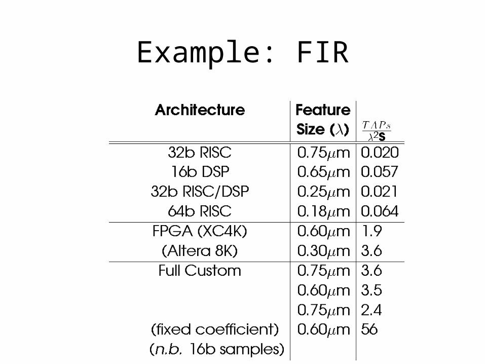
Example: FIR

Example: FIR

Example: DNA/Splash Revisited

Area-Time Curves

• Simple performance density picture complicated by:– Non-ideal area-time curves– Non-scalable designs– Limited parallelism– Limited throughput requirements

AT Example: FIR

Characterization

• Performance alone doesn’t tell the story

• Need to track: – resource requirements

• e.g. CLBs, components

– absolute compute time– energy– technology

• Scaling (A-T) curves are beneficial

Summary

• To conquer confusion:– compare FPGA-based computations with alternative

implementation technologies– take care in comparison to normalize

• Many reasons for choosing a technology beyond cost/performance– always want to know what you’re paying for what

you get