International Journal of Forecasting 7 (1991) 403-406

North-Holland

403

Teaching tips

The paper below continues Te&ing t$.r, a new section of the journal. Its purpose is to allow instructors to share ideas relevant to the teaching of forecasting, at any level of instruction. To be considered for publication, a teaching tip need only have been employed successfully by the author (or others); there is no requirement that allegations of its effectiveness be supported by hard empirical evidence. Other than that submissions be brief, there is no restriction on their form or content. To give some examples, a tip could be a novel graphical expostion, an effective assignment question, a stimulating learning game, a particularly good example, an imaginative computer exercise, or a successful class project, which in the author’s experience has proved to possess significant pedagogical value, at any level of instruction. Referees will be asked to evaluate papers in terms of their potential for improving the teaching of forecasting. Submissions should be sent, in triplicate, to Peter Kennedy, Department of Economics, Simon Fraser University, Burnaby, B.C., Canada WA 1%.

Comparing classification techniques

Peter Kennedy

An interesting variant of forecasting in the con- text of cross-sectional data is the classification problem: Given observations on attributes of an object, classify it to one of two or more mutually exclusive and exhaustive categories. For example, given measurements on various relevant charac- teristics of a firm, should its shares be classified as ‘buy’ or ‘not buy’? The purpose of this note is to discuss briefly the three most popular classifi- cation techniques, linear discriminant analysis, logistic regression, and goal programming, and to present a graph illustrating their differences. For expositional reasons, the discussion is confined to the case of binary choice.

Suppose an object to be classified belongs to either group 1 or group 2 and that a vector w of attributes of this object is available. A classifica- tion rule is called ‘optimal’ if it classifies an object to the group for which the probability of its belonging is greatest. From theoretical considera- tions, each of the three techniques exposited in

this note can be shown to be ‘optimal’ in special situations.

Linear discriminant analysis

Suppose the attribute vector w is distributed as a multivariate normal, with mean p, or p.2 and common covariance matrix 2, depending on whether the observation is from group 1 or group 2. If the prior probabilities are equa1 (which we assume throughout), the optimal classification rule is to classify an observation group 1 if 6 + p’w > 0 and to group 2 if not , where 6 + p’w is the linear discriminant function, with 6 = (~,‘Z~l~Z -~,‘Z-‘~r) and 8 = 2tpr - ~z)‘X-i. This method is operationalized by using the indi- vidual sample means and a weighted (by sample size) average of the individual sample variances to estimate the pi and 2.

0169-2070/91/$03.50 Q 1991 - Elsevier Science Publishers B.V. All rights reserved

This rule can be derived by maximizing the relevant likelihood ratio, as in Anderson (1984, pp. 204-206). The same rule results from finding the linear combination of the attributes that max- imizes the ‘distance’ between the two groups’ observations, as derived originally by Fisher (1936). The robustness of this rule to violations, such as the inequality of the covariance matrices or non-normality of the attribute vector, is not strong. Various techniques have been proposed to alleviate the impact of such violations, such as adjustments to the estimate of the constant term 6 suggested by Knoke (1982).

Logistic regression

If the probabilities of belonging to groups 1 and 2 are such that the logarithm of their ratio is a linear function in w, say (Y + /3’w, the logistic regression classification technique is optimal, with the probability of belonging to group 1 given by exptcu + 0’w)/(l + exp(a + f3’w)). An observa- tion is classified to group 1 if this probability exsceeds one-half, otherwise it is classified to group 2. This rule is usually operationalized through maximum liklihood estimation of the un- knowns. For discussion of its optimality proper- ties see Day and Kerridge (1967, pp. 313-315). Types of w variables for which this optimality property holds are multivariate normal variables with equal covariance matrices, independent and dichotomous zero/one variables, and mixtures of multivariate normal and dichotomous variables. The normal is not the only exponential family satisfying this optimality property.

The condition for optimality of linear discrimi- nant analysis, w distributed multivariate normally with equal covariance matrices, is a special case of the condition for optimality of the logistic regression approach. Hence logistic regression should be more robust than linear discriminant analysis, and this may explain why most studies comparing the two have shown logistic regression to be superior. Malhotra (1983) has a good sum- mary of this literature; Press and Wilson (1978) is a good representative of these studies, containing extensive discussion of the issues. In defence of linear discriminant analysis, Efron (1975) has noted that when the assumptions of the linear discriminant technique are met its operational

version will be more efficient asymptotically than the operational version of logistic regression, be- cause it exploits these assumptions when estimat- ing the unknown parameters.

The logistic model can also be derived from the random utility model. Suppose an individual chooses between the two alternative classes on the basis of the utility U, and CJZ each provides, where the U[ are linear functions of w plus a stochastic term. As shown by McFadden (1974), if the stochastic term is distributed as an indepen- dent Weibull, the probability that U, > U2 takes the logistic form. This suggests that logit analysis might perform well in a context in which the data is likely to have been generated by some kind of conscious choice mechanism linked to utility max- imization.

Goal programming

Assume that a linear function of the form A + 4’~ 2 1 for an observation from group 1 and A + 4’~ 5 - 1 for an observation from group 2 can separate the two classes. Since it is usually impossible to achieve perfect discrimination, two zero/one dummy variables, d and e, are intro- duced such that d or e takes the value one for a misclassification and zero otherwise. Multiplying these dummies by an arbitrarily-chosen large number M leads to the constraint A + 4’~ + Md 2 1 for each group 1 observation and the con- straint A + +‘w - Me I - 1 for each group 2 ob- servation, all of which are capable of being satis- fied. The sum over all the observations of the d’s and e’s measures the total number of misclassifi- cations, which is to be minimized. Thus the goal programming problem is to minimize the sum of the d’s and the e’s, subject to the constraints above, with respect to A, 4, the d’s and the e’s. Doing this while forcing the d’s and e’s to be zero/one integers is called integer goal program- ming. An observation is classified to group 1 if for that observation the estimated A + 4’~ 2 0. For a more detailed description, see Choo and Wed- ley (1985).

Unfortunately, when d and e are constrained to be zero/one integers, goal programming is computationally more expensive than the other methods (by a factor of about 100); whenever there are more than ten misclassifications using

Teaching t1p.s 405

logistic regression or linear discriminent analysis, as is likely whenever the sample size is large, integer programming can become prohibitively expensive and thus may not be feasible. An alter- native is to set M equal to one and allow d and e to take non-integer values; rather than weighting each misclassification equally, in this approach misclassifications contribute to the objective func- tion in proportion to their distance from the classification surface. This variant, non-integer goal programming, may provide a computation- ally inexpensive approximation to the superior but expensive integer goal programming.

Two conditions, discussed in Hand (19811, are required for integer goal programming to be opti- mal: The optimal decision surface must be linear in w and the sample must be perfectly represen- tative of the parent population. Goal program- ming implicitly uses the sample to estimate the probability density function of the parent, so the larger the sample the better. This suggests that integer goal programming will be more robust than the linear discriminant function as the sam- ple size increases - integer goal programming should be able to find the optimal decision sur- face whenever it is linear, whereas the linear discriminant function will only do so when the attribute vector is distributed normally with iden- tical covariance matrices. Should this latter con- dition hold, though, the linear discriminant func- tion should be superior asymtotically since it ex- ploits this information in its estimation.

In their response to Glorfeld and Gaither (1982), who argue against programming tech- niques, Freed and Glover (1982) present a strong case, summarized in Glover, Keene and Duea (1988), for the use of linear programming tech- niques for classification purposes. In the absence of extraneous information, such as that the sub- groups are distributed normally, the main a priori appeal of goal programming is that, in contrast to other methods, it forms its decision rule by mini- mizing the number of misclassifications, which may be of direct interest. It must be noted that this may not be of primary interest, however; it may be that interest centers on the extent to which a change in an attribute affects the proba- bility of being in group 1, in which case the parameter estimates provided by the logit ap- proach would be of most value.

A graphical interpretation

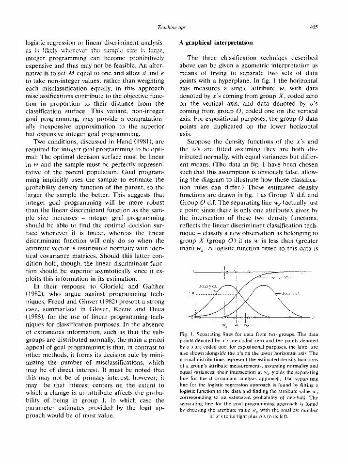
The three classification techniqes described above can be given a geometric interpretation as means of trying to separate two sets of data points with a hyperplane. In fig. 1 the horizontal axis measures a single attribute W, with data denoted by x’s coming from group X, coded zero on the vertical axis, and data denoted by o’s coming from group 0, coded one on the vertical axis. For expositional purposes, the group 0 data points are duplicated on the lower horizontal axis.

Suppose the density functions of the x’s and the o’s are fitted assuming they are both dis- tributed normally, with equal variances but differ- ent means. (The data in fig. 1 have been chosen such that this assumption is obviously false, allow- ing the diagram to illustrate how these classifica- tion rules can differ.) These estimated density functions are drawn in fig. 1 as Group X d.f. and Group 0 d.f. The separating line w, (actually just a point since there is only one attribute), given by the intersection of these two density functions, reflects the linear discriminant classification tech- nique - classify a new observation as belonging to group X (group 0) if its w is less than (greater than) wd. A logistic function fitted to this data is

Fig. 1. Separating lines for data from two groups. The data

points denoted by x’s are coded zero and the points denoted

by u’s are coded one; for expositional purposes, the latter are also shown alongside the x’s on the lower horizontal axis. The

normal distributions represent the estimated density functions

of a group’s attribute measurements, assuming normality and

equal variances; their intersection at wd yields the separating

line for the discriminant analysis approach. The separating

line for the logistic regression approach is found by fitting a

logistic function to the data and finding the attribute value W, corresponding to an estimated probability of one-half. The

separating line for the goal programming approach is found

by choosing the attribute value wK with the smallest number of x’s to its right plus O’S to its left.

also shown in fig. 1. The logistic regression classi- fication technique classifies a new observation to group X (group 0) if its w is such as to make the fitted logistic function less than (greater than) one half. This yields the separating line w,. The goal programming classification technique finds a separating line that minimizes the total number of misclassifications - the number of o’s on its left plus the number of x’s on its right. An arbitratry choice mechanism solves the non- uniqueness problem and yields the separating line wx.

Although as discussed above each of these three classification techniques is optimal for cer- tain data generation mechanisms, unfortunately there is no consensus yet on which performs best overall on data likely to be encountered in prac- tice; in most applied studies their forecasting performances have not differed by much.

References

Anderson, T.W.. 1984. An Introduction fo Multimriule Stutis-

rid Anulysrs, second ed. (Wiley, New York).

Choo, E.U. and W.C. Wedley, 19%. “Optimal criteria weights

in repetitive multicriteria decision making”, Journal of the

Operutionul Research Society, 36, 983-992.

Day, N.E. and D.F. Kerridge, 1967, “A general maximum

liklihood discriminant”, Biometrics, 23, 313-323.

Efron, B., 1975, “The efficiency of logistic regression com-

pared to normal discriminant analysis”, Journal of the

American Staristical Sociefy, 70, 892-898.

Fisher, R.A., 1936. “The use of multiple measurements in

taxonomic problems”, Annals of Eugenics, 7, 179-188.

Freed, N. and F. Glover, 1982, “Linear programming and

statistical discrimination - The LP side”, Decision Sci-

ences. 13. 1722174.

Glover, F., S. Keene and B. Duea. 19X8, “A new class of

models for the discriminant problem”. Decision Sciences.

19. 269-280.

Glorfeld, L.W. and N. Gaither. 1982, “On using linear pro- gramming in discriminant problems“, Decision Sciences,

13, 167-171. Hand, D.J., 19X1, Discriminution and Classification (Wiley.

New York).

Knoke, J.D.. 19X2, “Discriminant analysis with discrete and

continuous variables”, Biometrics, 38. 191-200.

Malhotra. N.K., 1983, “A comparison of the predictive valid-

ity of procedures for analyzing binary data”, Journal of

Business and Economic Statisrics, 1, 326-336.

McFadden, D., 1974, “Conditional logit analysis of qualitative

choice behavior”. in: P. Zarembka, ed., I;‘rontlers in Econo-

metrics (Academic Press, New York) 105-142.

Press, S.J. and S. Wilson. 1978, “Choosing between logistic regression and discriminant analysis”, Journal ofthe Amrr-

ican Stutisticul A.s.wciation. 73, 699-70.5.