Comparative study of SBOAs on the tuning procedure of the ...

Delft University of Technology

Comparative study of SBOAs on the tuning procedure of the designed SMPI controller forMIMO VSP/HVDC interconnected model

Rakhshani, Elyas; Naveh, Iman Mohammad Hosseini; Mehrjerdi, Hasan

DOI10.1016/j.ijepes.2021.106812Publication date2021Document VersionFinal published versionPublished inInternational Journal of Electrical Power and Energy Systems

Citation (APA)Rakhshani, E., Naveh, I. M. H., & Mehrjerdi, H. (2021). Comparative study of SBOAs on the tuningprocedure of the designed SMPI controller for MIMO VSP/HVDC interconnected model. InternationalJournal of Electrical Power and Energy Systems, 129, 1-24. [106812].https://doi.org/10.1016/j.ijepes.2021.106812Important noteTo cite this publication, please use the final published version (if applicable).Please check the document version above.

CopyrightOther than for strictly personal use, it is not permitted to download, forward or distribute the text or part of it, without the consentof the author(s) and/or copyright holder(s), unless the work is under an open content license such as Creative Commons.

Takedown policyPlease contact us and provide details if you believe this document breaches copyrights.We will remove access to the work immediately and investigate your claim.

This work is downloaded from Delft University of Technology.For technical reasons the number of authors shown on this cover page is limited to a maximum of 10.

https://doi.org/10.1016/j.ijepes.2021.106812


Electrical Power and Energy Systems 129 (2021) 106812

Available online 16 February 20210142-0615/© 2021 Elsevier Ltd. All rights reserved.

Comparative study of SBOAs on the tuning procedure of the designed SMPI controller for MIMO VSP/HVDC interconnected model

Elyas Rakhshani a,*, Iman Mohammad Hosseini Naveh b, Hasan Mehrjerdi c

a Department of Electrical Sustainable Energy, Delft University of Technology, The Netherlands b Department of Electrical Engineering, Gonabad Branch, Islamic Azad University, Gonabad, Iran c Department of Electrical Engineering, Qatar University, Doha, Qatar

A R T I C L E I N F O

Keywords: Frequency control Virtual inertia Inertia emulation Optimal control Swarm – Based MPI (SMPI) Controller Swarm – Based Optimization Algorithms (SBOAs)

A B S T R A C T

This paper presents a new application of advanced SMPI controller for a newly introduced interconnected dy-namic system with VSP based HVDC links for frequency control problem. This work presents an outgrowth of analysis about the Swarm – Based Optimization Algorithms (SBOAs) in the tuning process of Multivariable Proportional – Integral (MPI) controller, which is called swarm – based MPI (SMPI). PSO, GOA and GWO al-gorithms are used for tuning process of the designed SMPI. The VSP based HVDC model is added for mitigation of system frequency dynamics with emulating virtual inertia. The proposed SMPI controller are designed for enhancing the dynamic performance of this system’s states during contingencies and they are compared with the conventional designed MPI controller. Deviation characteristics of the step function in MIMO transfer function of the VSP based HVDC model is considered as the common performance index in the proposed algorithms. On the other hand, the role of the proposed SMPI controller is to stabilize such interconnected system while minimizing the associated cost function. Matlab simulations next to the performed Nyquist’s stability anslysis demonstrate how the tuned SMPI can remarkably improve the frequency deviations and the damping of the inter-area os-cillations excited during a fault. This enhancement is more obvious especially when SMPI controller for a VSP based virtual inertia emulation is tuned using GWO method.

1. Introduction

The rapid evolution and expansion of the existing AC network into an interconnected low-inertia scenario with a high share of renewable- based generation units, is leading to a system with high complexities, which can impact the dynamics of the overall network and particularly the frequency stability of AC/DC interconnected modern system [1]. AC/DC system mainly consists of hybridization of the common Alter-native Current (AC) based network and the Direct Current (DC) based components. Nowadays, thanks to significant advancement in power electronic technologies, it became possible to use high-voltage DC (HVDC) transmission systems and power electronic-based components in a very effective manner. HVDC systems overcome the main draw-backs of HVAC transmission, especially for a very long distance appli-cation. The frequency control mechanism for such a multi-area modern system, during load and resource variation, is very important. It can consist of primary and secondary frequency control. Primary control is referring to the inertial response of the governors against the frequency

mismatch. Its main role is to provide enough inertia for maintaining the stability of the system especially within the next couple of seconds after the frequency drop. Secondary frequency control or AGC is a higher- level control mechanism that can facilitate different tasks such as fre-quency restoration, tie-line power flow control between authority areas and economic dispatch of generation units [2]-[3]. The interconnection of multi areas can be supported by AC lines of HVDC tie-lines which can enable the transfer of the scheduled power between different zones. It can also give more support and back up to the neighboring area in abnormal situations. Considering the operation limitations of AC lines especially for long-distance, the DC transmission is receiving increasing attention over the last recent years.

HVDC links are known as one of the main utilization of power electronics in modern power systems, which could convey several ad-vantages such as fast and bidirectional control on active and reactive power, power oscillation damping and frequency stability support [4,5]. With proper coordination, they can improve the reliability of complex systems and can act as a kind of firewall against cascading disturbances. Due to these advantages, in many projects, the DC links or hybrid AC/DC

* Corresponding author. E-mail addresses: [email protected] (E. Rakhshani), [email protected] (H. Mehrjerdi).

Contents lists available at ScienceDirect

International Journal of Electrical Power and Energy Systems

journal homepage: www.elsevier.com/locate/ijepes

https://doi.org/10.1016/j.ijepes.2021.106812 Received 5 August 2020; Received in revised form 13 October 2020; Accepted 12 January 2021

mailto:[email protected]

mailto:[email protected]

www.sciencedirect.com/science/journal/01420615

https://www.elsevier.com/locate/ijepes




http://crossmark.crossref.org/dialog/?doi=10.1016/j.ijepes.2021.106812&domain=pdf

International Journal of Electrical Power and Energy Systems 129 (2021) 106812

2

interconnections are becoming the preferred option [6–7]. Recently, several attempts have been made in the control of grid

connected power converted for enhancing the dynamics of low-inertia AC/DC systems by providing virtual inertia to the grid [8–9].

The virtual inertia is emulated by using advanced control of power converters considering their short term energy storage, [10] which gives rise to the possibility of having a higher amount of distributed genera-tion systems, connected to the grid through power converters, without hindering the system stability. However, the application of this kind of converters are not restricted to low power applications or generation parts. For instance, it can be a beneficial option for HVDC power con-verters. As reported in [11], a novel technique, named VSP based HVDC system, is introduced for inertia emulation capability. Up to now, only the basic model and its mathematical model are reported while no further improvements in tuning and its optimal operation have been reported yet. The AC/DC interconnected system with VSP capabilities is a complex MIMO system that suffers from the lack of advanced control methodology for better operation of the VSP based HVDC system. This paper is trying to fill this gap by proposing a heuristic-based MPI controller for such a system.

Recently, different control methods are presented to achieve accu-rate and suitable damping effects, such as sliding mode control (SMC) [12–14]. SMC is basically a roust control technique that is used to control systems with uncertainties. The biggest advantage an SMC possess over PID is the finite-time stability of the closed-loop system (may not be true for discrete time systems). Another important point to remember is that the SMC can reject the disturbances (disturbance decoupling, when properly designed), whereas PID can reduce or remove the effect of uncertainties. In the most common sliding mode control schemes the main limitation is that the performance of the controller relies on the sliding surface. If the sliding surface of SMC is not designed properly, it may lead to unacceptable performance while the applications in real practice is not easy.

Among the controller variety, Proportional-integral (PI) becomes the controller that is most common and the most applied in a physical sys-tem [15]. The reason is that it has a characteristic that offers simplicity, clear functionality, and ease of use [16]. However, Ho et al. [17] re-ported that only one-fifth of PI control loops are in good condition. The others are not, where 30% of PI controllers are not able to perform well due to the lack of tuning parameters, 30% due to the installation of a controller system operating manual, and 20% due to the use of default

controller parameters. In recent years, many researchers have paid attention to the MPI

controllers design for various systems such as in Industrial Scale - Polymerization Reactor [18], Coupled Pilot Plant Distillation Column [19], Narmada Main Canal [20], Quadruple-Tank Process [21], Boiler- Turbine Unit [22], and Wood-Berry Distillation Column [23]. Research by Kumar et al. [18] had proposed a synthesis based on the approximation of the relative gain array (RGA) concept to the multi-variable process.

The method was further improved by relative normalize gain array concept (RNGA). The controller based on RNGA concept provides better performance than the RGA concept. Both concepts use the nonstandard PI controller which requires Maclaurin series expansion [24]. Multi-variable PI or PID controller utilization, by attention to all its advan-tages, has been reported, specifically on industrial applications, as a method in several scientific societies. For achieving a safe, robust and flexible strategy for optimal coefficients arrangement a meta – heuristic based algorithms, has been discussed frequently [25–31]. It should be mentioned that the utilized cost functions in these works are focused on the different index such as ITAE and ISE. Some of the main limitations in these mentioned papers are the need for high availability and direct access to the state variables while the distortion of the measurable state variables with the noise is an additional burden in actual implementation.

But in this paper, by attention to the determined features of the step response and its accessibility in every iteration of the simulation, a fitness index is used according to the extracted features of the step function. Also by considering the variety of intelligent optimization al-gorithms in the tuning process, it is necessary to review all methods as comparative researches. The utilization of swarm–based optimization algorithms, specifically GOA and GWO, will increase the convergence performance in comparison with the applied typical MPI tuning [32–37]. MPI controller has few parameters to adjust and is relatedly simple to implement. It’s robust and can be used in parallel computa-tion. The advantage and necessity of MPI controller are on its feasibility and easy to be implemented. The MPI gains can be designed based upon the MIMO system parameters if they can be achieved or estimated precisely. Moreover, the MPI gain can be designed just based on the system tracking error and treats the system to be “black-box” if the MIMO system parameters are unknown. However, the MPI controller generally has to balance all matrix-gains impact on the whole system and may compromise the transient response. Thus, a complementary action from heuristic based algorithm for such a controller can advance the performance of the controller. This is another important topic that going to be answered, for interconnected system with VSP, in this paper.

The application of swarm based algorithm for better tuning of MPI approach is a very interesting idea which can further enhance the per-formance of the controller. The first and the most basic presented defi-nition for “swarm” is based on a similar and simple set of agents that are interconnected locally among themselves. So by considering the above explanation, swarm – based optimization algorithms (SBOAs) have been introduced as a subset of nature – inspired, crowd – based algorithms which are able to generate low cost, fast and robust solutions for an extensive set of the multiplex problems. Simultaneous to introduce swarm – based computational models, there has been a mutation in the number of scientific activities which presented the successful utilization of SBOAs in a various set of optimization tasks and complex problems. SBOA principles have been successfully achieved in a variety of prob-lems consist of function and structural optimization, finding optimal routes, scheduling and image and data analysis. Swarm – based Computational models have been further used in a wide-range of diverse domains, involving machine learning, bioinformatics and medical informatics, dynamical systems and operations research. Until now, several AI algorithms are performed for achieving to an optimal tuning coefficients method, such as Artificial Bee Colony [38] and Ant Colony algorithm [39–41] which are applied in the tuning process of MPI

Nomenclature:

ACE Area Control Error AGC Automatic generation control GOA Grasshoppers Optimization Algorithm GWO Grey Wolf Optimization HVDC High Voltage Direct Current MI Multivariable Integral Controller MIMO Multi Input Multi Output MP Multivariable Proportional Controller MPI Controller Multivariable PI Controller PI Controller Proportional – Integral Controller PSO Particle Swarm Optimization SBOAs Swarm – Based Optimization Algorithms SI Stability Index SMPI Controller Swarm – Based Multivariable Proportional –

Integral Controller ST Settling Time Index RT Rise Time Index VSP Virtual synchronous power VSP/HVDC VSP - Based HVDC Model

E. Rakhshani et al.


3

controllers. These AI algorithms are created based on a simple structure and therefore they cover some of the optimization problems which are performed for uncomplicated systems.

In this work, a new application of heuristic-based MPI controller design for AC/DC interconnected system with VSP capabilities is pro-posed. This control approach is based on the evolutionary-based swarm intelligence (SI) optimization algorithms. Particle Swarm Optimization (PSO), Grasshoppers Algorithm (GOA) and Grey Wolf Optimization (GWO) are the main SBOAs, which are used for the tuning process of MPI controller. The focus of this study is on a new design of advanced control for VSP concept through the converter stations of HVDC link, which is achieved by means of an SMPI controller in a multi-machine AGC system.

Another importance of the proposed approach is on the proposition of a unique performance index as part of the optimization process. The performance index is defined as a function consists of a linear combi-nation of step response features such as stability index (SI) and settling time (ST). Finding the best MPI coefficients, as the main target among this process, is realized using the minimization of the proposed perfor-mance index.

The proposed advanced control approach is validated through the Matlab simulations of an interconnected AGC dynamic model with HVDC with the VSP capabilities. The proposed method is based on the minimization of a performance index, which is designed by attention to the transfer function characteristics matrix in an MIMO system. The MPI controller design method is performed on the systems to enhance the characteristics performance model versus the conventional PI controller method.

The rest of the paper is organized as the following. In the next sec-tion, Section 2, the mathematical formulation of the studied two-area interconnected AGC dynamic model, consists of a detailed model with DC link with VSP capabilities, with an MIMO transfer function charac-teristics are discussed. Then, in the next Section 3, a typical MPI

controller design considering the tuning of its coefficients are presented. In Section 4 swarm-based optimization algorithms (SBOA) considering PSO, GOA and GWO insertions are explained. The simulation results for VSP-HVDC and AC/HVDC model are presented in Section 5. In this section, the robustness of the controller against parameter changes with Nyquist analysis is also presented and compared. Finally, the conclu-sions and controller remarks are presented in Sections 6.

2. VSP-based AC/HVDC interconnected system

In this section, the concept of VSP for inertia emulation through the converter stations of the HVDC links in a two-area system will be presented.

2.1. Dynamic model of the VSP facilitated system

We deploy a high-level control architecture to simulate and analyze the frequency behavior of the AC/HVDC two-area system equipped with VSP functionalities. In general, the VSP strategy is based on the control of voltage source converters through an active power synchronization loop and a virtual admittance [11].

After an analysis of the electromechanical model of the VSP, the dynamic relationship between input and output power of each converter station could be a second-order transfer function. Then a characteristic equation of the VSP dynamic model can be derived for the description of this second-order system, namely,

y + 2ζωny + ωn2 = ωn

2u (1)

where ζ is the damping factor,ωn is the natural frequency. The input signal, u, is the reference DC power which is related to other states of the global multi-area system. The output signal consists of two states variables:

Fig. 1. Basic frame of AGC in multi-area systems with a VSP based AC/DC transmission.

E. Rakhshani et al.


4

ΔYvsp =

[Δxp,vspΔxf,vsp

]

(2)

where Δxp,vsp represents the injected DC power and Δxf,vsp is the de-rivative term of this power for each VSP, respectively. Based on classic control concepts, this second-order system could be represented by a set of two linear state equations: [

Δxp,vspΔxf,vsp

]

=

[0 1

-ωn2 -2ζωn

][Δxp,vspΔxf,vsp

]

+

[0

ωn2

]

Δu (3)

where Δu denotes the input signal of the DC power reference (ΔPDC, ref) that comes from a higher-level control. Here Δu is generated by other control signals. For a two-area interconnected system with Area i and Area k, let us assume that a VSP based HVDC link is implemented. As the HVDC line is located between these two areas, the frequency deviation of each area is the most suitable control signal. In the case of parallel AC/DC lines, the AC tie-line power deviation could be used as another control signal in order to achieve suitable coordination between these two lines. Thus we can have:

Δu = Kfi,vspΔωi + Kfk,vspΔωk + KACΔPtieAC,ik (4)

where Kfi,vsp, Kfk,vsp and KAC are the proportional coefficients for the frequency deviations Δωi, Δωkand AC power flow deviations ΔPtieAC,ik of these two areas, respectively.

This state space presentation in (3) will be part of the global model for the frequency dynamics of the two-area AC/DC system with VSP- based inertia emulation. Fig. 1 depicts the high-level control structure of the two-area system with a VSP-based AC/DC transmission. For the frequency regulation, typically a low-order linearized model could be used for modeling the load-generation dynamic behavior, namely the AGC model. Thus to study the small-signal modeling and stability of the high-level control design, we can describe the dynamic equations of these two AC/DC interconnected areas considering the dynamics of the VSP-based HVDC link in the Laplace domain as follows:

Δωi =Kpi

(ΔPmi-ΔPli-

(ΔPtieACi + Δxp,vspi

) )

1 + sTpi(5)

Δωk =Kpi

(ΔPmk-ΔPlk-

(ΔPtieACk-Δxp,vspk

) )

1 + sTpk(6)

where ΔPmi and ΔPmk denote total active power from all generation units (GENs) within Area i and k, respectively.

The part of AGC control calculates the Area Control Error (ACE) of Area i. The ACE signal now contains the frequency deviations of that

area and both AC/DC power flow deviations, and acts as the input for an integral control action,

ACEi = βiΔωi +[ΔPtieACi +Δxp,vspi

](7)

ACEk = βkΔωk +[ΔPtieACk − Δxp,vspk

](8)

where for Area i, βi is the frequency bias. In (5) and (6), the parts Δxp,vspi

and Δxp,vspk denote the total output of the VSP based DC transmitted power. Thus for this one VSP station on the HVDC line in the two-area system, the following equations can be further derived from (3),

sΔxp,vspi = Δxf,vspi (9)

Δxf,vspi = αiΔωi + αkΔωk + αikΔPtieACik − ωni2Δxp,vspi − 2ζωniΔxf,vspi (10)

sΔxp,vspk = Δxf,vspk (11)

Δxf,vspk = γiΔωi + γkΔωk + γikΔPtieACik − ωnk2Δxp,vspk − 2ζωnkΔxf,vspk (12)

where ⎧⎪⎪⎪⎪⎪⎪⎪⎪⎪⎪⎨

⎪⎪⎪⎪⎪⎪⎪⎪⎪⎪⎩

αi =Kfi,vspωni

2

2π

αk =Kfk,vspωni

2

2π

αik = KAC,vspωni2

(13)

and ⎧⎪⎪⎪⎪⎪⎪⎪⎪⎪⎪⎨

⎪⎪⎪⎪⎪⎪⎪⎪⎪⎪⎩

γi =Kfi,vspωnk

2

2π

γk =Kfk,vspωnk

2

2π

γik = KAC,vspωnk2

(14)

2.2. Mathematical state-space VSP-HVDC model

As it is mentioned in Section 2.1, we can have a global linearized mathematical representation of the two-area AC/DC interconnected power system with VSP-based inertia emulation strategy:

Fig. 2. A two-input two output system block diagram.

E. Rakhshani et al.


5

⎧⎪⎪⎨

⎪⎪⎩

Δxvsp(t) = Avsp(13×13)Δxvsp(t) + Bvsp

(13×2)Δuvsp(t)

Δyvsp(t) = Cvsp(2×13)Δxvsp(t)

(15)

Δxvsp =

⎡

⎣Δω1 Δω2 ΔPm1 ΔPm2 ΔPm3 ΔPm4

ΔACE1 ΔACE2 ΔPtieAC12Δxp,vsp1 Δxf,vsp1 Δxp,vsp2 Δxf,vsp2

⎤

⎦

T

(16)

Δuvsp = [ΔPl1 ΔPl2]T (17)

Δyvsp = [Δω1 Δω2]T (18)

All of the required coefficients and constant values are available in [42–43].

2.3. MIMO transfer function characteristics

As it was mentioned in this work, simulation results and conclusions will be presented as a MIMO system. Therefore, it is necessary to review this type of systems, specifically as a two-input two-output model. For achieving a common understanding about MIMO system, assume the following block diagram shown in Fig. 2. As it is observed, this figure represents a MIMO system as a two-input two-output model.

By attention to above block diagram, it can obtain: ⎧⎨

⎩

Y1(s) = G11(s)U1(s) + G12(s)U2(s)

Y2(s) = G21(s)U1(s) + G22(s)U2(s)(19)

[Y1(s)Y2(s)

]

=

[G11(s) G12(s)G21(s) G22(s)

][U1(s)U2(s)

]

(20)

So (19) can be rewrite as a matrix form: [

Y1(s)Y2(s)

]

=

[G11(s) G12(s)G21(s) G22(s)

][U1(s)U2(s)

]

(21)

By considering to the applied controllers in this MIMO model, it can obtain: {

U1(s) = GC1(s)E1(s)U2(s) = GC2(s)E2(s)

(22)

By replacing (20) in (21): [

Y1(s)Y2(s)

]

=

[G11(s)GC1(s) G12(s)GC2(s)G21(s)GC1(s) G22(s)GC2(s)

][E1(s)E2(s)

]

(23)

Also: {

E1(s) = R1(s) − Y1(s)E2(s) = R2(s) − Y2(s)

(24)

Therefore, it can be obtained as follows:

and:

By replacing and simplifications (19) – (23), finally we can achieve to the MIMO transfer function for a two – inputs two – outputs model: [

Y1(s)Y2(s)

]

=

[T11(s) T12(s)T21(s) T22(s)

][R1(s)R2(s)

]

(27)

where Tij (i,j = 1,2) are the main elements of transfer function matrix which are calculated individually as follow:

T11(s) =G11(s)GC1(s) + GC1(s)GC2(s)(G11(s)G22(s)-G12(s)G21(s) )

d(s)(28)

T12(s) =G12(s)GC2(s)

d(s), T21(s) =

G21(s)GC1(s)d(s)

(29)

T22(s) =G22(s)GC2(s) + GC1(s)GC2(s)(G11(s)G22(s)-G12(s)G21(s) )

d(s)(30)

where

d(s) = (1 + G11(s)GC1(s) )(1 + G22(s)GC2(s) )-G12(s)G21(s)GC1(s)GC2(s)(31)

And for MPI controller: ⎧⎪⎪⎪⎪⎨

⎪⎪⎪⎪⎩

GC1(s) = K1 +K2

s

GC2(s) = K3 +K4

s

(32)

Finally, by considering the described equations, MIMO transfer function for VSP/HVDC model can be driven as follows:

GvspTotal(s) = Cvsp

(2×13)

(SI - Avsp

(13×13)

)-1Bvsp

(13×2) (33)

[Δω1(s)Δω2(s)

]

=

[Gvsp

11 (s) Gvsp12 (s)

Gvsp21 (s) Gvsp

22 (s)

][ΔPL1(s)ΔPL2(s)

]

(34)

It is possible to calculate MIMO transfer function for VSP/HVDC model by attention to all constant values in the steady state model (15) and calculation matrixes Avsp, Bvsp and Cvsp. The obtained transfer functions are presented in Appendix A.

Fig. 3. Block diagram of a MIMO system.

[Y1(s)Y2(s)

]

=

[1 + G11(s)GC1(s) G12(s)GC2(s)

G21(s)GC1(s) 1 + G22(s)GC2(s)

]− 1[G11(s)GC1(s) G12(s)GC2(s)G21(s)GC1(s) G22(s)GC2(s)

][R1(s)R2(s)

]

(26)

[1 + G11(s)GC1(s) G12(s)GC2(s)

G21(s)GC1(s) 1 + G22(s)GC2(s)

][Y1(s)Y2(s)

]

=

[G11(s)GC1(s) G12(s)GC2(s)G21(s)GC1(s) G22(s)GC2(s)

][R1(s)R2(s)

]

(25)

E. Rakhshani et al.


6

3. Typical MPI controller design

The typical tuning process of an MPI controller for a linear multi-variable stable plant is introduced in [44–45]. Therefore, the obtained MPI controller coefficients from this method, (KP and KI), can be determined by notification to the tuning MP controller coefficient (KP).

3.1. Tuning of MP coefficient

As it was mentioned, for finding KP and KI in MPI controller based on the typical method, it is necessary to determine KP as the main coeffi-cient in MP controller. As Fig. 3, the MIMO system in the existence of a general controller, as GC, can be illustrated.

By attention to Fig. 3 and considering MP controller for GC(s), it can be seen:

u(s) = KP . e(s) (35)

Then by considering steady state model for the main plan, it is rep-resented by:

x(t) = (A-BKPC)x(t) + BKPu(t) (36)

By assumption initial conditions:

x(t) = e(A-BKPC)t∫t

0

e-(A-BKPC)τBKP(τ)dτ (37)

Therefore, we have:

x(t) = -(A-BKPC)-1BKPr + e(A-BKPC)t(A-BKPC)-1BKPr (38)

By replacement to the state equation:

y(t) = -C(A-BKPC)-1BKPr + Ce(A-BKPC)t(A-BKPC)-1BKPr (39)

By attention to Fourier series definition:

y(t) = CBKPrt + C

[∑∞

k=2(A-BKPC)k tk

k!

]

BKPr (40)

By considering t = 0:

y(t) = CBKPrt (41)

where KP matrix is given by:

KP = (CB)+⎡

⎣k1 ⋯ 0⋮ ⋱ ⋮0 ⋯ km

⎤

⎦ (42)

where (CB)+ is the left inverse matrix for CB and it is given by:

(CB)+ = BTCT( CBBTCT)-1 (43)

It is important to know that in the square matrix:

(CB)+ = (CB)-1 (44)

Finally, by attention to (41) – (43) and selection k1,…,km, KP will be achieved in (41).

3.2. Tuning of MI coefficient

In this section the control signal, considering the assumed MI controller in Fig. 3 and the equation of GC(s) = KI/s, will be achieved:

u(s) =KI

s. e(s) (45)

Now by definition z(t) =∫ t

0 e(τ)dτ, the closed-loop system equa-tions will be arranged as:

[

Δx(t)Δz(t)

]

=

[A BKI-C 0

][Δx(t)Δz(t)

]

+

[0I

]

r(t) (46)

So the stable of closed-loop system will be guaranteed by: ⎧⎨

⎩

limt→∞

z(t) = 0

limt→∞

x(t) = 0(47)

And finally, when the state matrix is square then the coefficient KI is achieved by:

KI = G-1(0) (48)

where,

G(0) = − CA− 1B (49)

Cnsidering Section 3.A and 3.B, also (40) - (44), the conventional MPI (MP + MI) coefficients are available for achieving.

4. Swarm – Based optimization algorithms (SBOAs)

As explained in the introduction, SBOAs can be called as an indi-vidual branch of artificial intelligence (AI) which are applied to imple-ment the communal behavior of social swarms in nature. The social interconnections between swarm individuals can be either direct or in-direct [46–48]. The waggle dance of honey bees can be introduced as an example of direct interconnection which is through visual or audio contact. When one individual can change the situations in its around environment, actually indirect interconnection happens. Also, the other individuals answer to the new environment, such as the pheromone trails of ants that they settle on their way to search for food sources.

In every swarm – based algorithm, it is actually important to address the exploration and exploitation of a search space. The process of encountering new regions of a search space is called the exploration process. Also the process of encountering those regions of a search space within the neighborhood of previously visited points, will be introduced as exploitation process. For achieving to the specific targets and have a successful search algorithm, it is necessary to design a suitable ratio between exploration and exploitation. Fig. 4 can describe these two management concepts by attention to the nature of algorithms. As it is mentioned, some algorithms, such as Steepest Descend, Gradient and Newton Raphson, are located so closed to the vertical axis (exploitation parameter). These algorithms are so depended on the start point. In the other hand, if they have been tuned from suitable start point then the optimization process will be finalized to the best answer. Therefore, such

Fig. 4. Search space management in algorithms based on exploration and exploitation.

E. Rakhshani et al.


7

algorithms direct the process greedily. But on the contrary, those algo-rithms which are so close to the horizontal axis (exploration parameter), will be based on random searches. In the other hand, every algorithm which emphasizes exactly to the exploration parameter, will be impractical in the optimization process.

By considering the above descriptions, it is obvious that a SBOA can be achieved to find the best answer when it uses a correct combination between these two factors.

SBOAs are known as a subset from a bigger set which are called meta - heuristic methods. A meta - heuristic is a high-multiplex problem that presents a set of strategies to expand heuristic optimization algorithms.

Meta - heuristics have been demonstrated by the scientific commu-nity to be a viable, and often superior, alternative to more traditional (exact) methods of mixed integer optimization such as dynamic pro-gramming. By attention to the recently obtained experiences in complicated or large problem, meta - heuristics are capable to give a suitable trade - off between solution quality and computing time. Fig. 5 presents a total scheme from the metaheuristic algorithms classification based on the nature of applied methods.

As it was described, SBOAs will be classified as one of the most important subsets. By attention to this scheme, Particle Swarm Opti-mization (PSO), Grasshoppers Algorithm (GOA) and Grey Wolf Opti-mization (GWO) are the main SBOAs, which are performed in this work.

4.1. Particle swarm optimization (PSO)

This methodology, as the first and the most developed SBOAs, is a meta - heuristic approach inspired by the individual and social behavior of the flocking birds [49]. In PSO algorithm, particles are known as the population of candidate solutions in optimization problem. Each one of particles is determined by means of two important components which are position and velocity vectors. In this method, every particle tracks its direction towards the total optimum based on Newtonian mechanics. The particle components are defined for the ith particle and in a D - dimensional space:

x→i(t) = [xi1(t)xi2(t)⋯xiD(t) ]T (50)

v→i(t) = [vi1(t)vi2(t)⋯viD(t) ]T (51)

Also, the upgrade rules in this algorithm, according to the compo-nents are illustrated below equations respectively:

v→i(t+ 1) = w v→i(t)+ c1r1

(

x→pbi − x→i(t))

+ c2r2

(

x→g − x→i(t))

(52)

x→i(t+ 1) = x→i(t)+ v→i(t+ 1) (53)

where × and v are the main components in PSO algorithm. w is applied inertia to achieve the convergence speed and balance between exploi-tation and exploration. c1 and c2 are two positive constants and r1 and r2 are random numbers obtained from a uniform random distribution function in the interval [0,1]. xpbi is the best position that ith particle have seen and xg is the position of the best particle seen so far among the upgrade process.

4.2. Grasshopper optimization algorithm (GOA)

Grasshoppers are classified as a set of insects which generally harm

Fig. 5. Metaheuristic algorithms classification.

Fig. 6. Conceptual movement in a swarm of grasshoppers.

E. Rakhshani et al.


8

to the crop production as they consider as a kind of agriculture pest. These kinds of insects are usually seen individually in out around environment but mostly they fly as a large swarm in nature. The swarm of grasshopper has one distinctive feature which is its swarming behavior in both the nymph as well as adulthood in grasshopper. The nymph grasshopper flies like rolling cylinders in millions of numbers. Grasshoppers destroy all the vegetation which exists on their path dur-ing their motion. After nymph - hood, they become adult and gradually create a swarm in air and then they flight over a very large distance.

In the swarm larval – hood, the swarm of grasshopper generally has a very slow moving. The basic feature in the larval – hood is the small step of the grasshopper. Unlike this duration, the most important feature of swarm in adulthood is long range and sudden motion of swarm. The grasshopper swarm mostly create for the finding of food source. This searching process is another important characteristic for the swarm of grasshopper. As it was explained in the introduction paragraph, explo-ration and exploitation are two important determined factors in SBOA. Both tendencies are enhanced by grasshoppers naturally in which they fly abruptly as well as locally in small areas.

A scientific model is performed of this behavior of grasshopper swarm to design a nature-inspired optimization algorithm. This math-ematical model utilizes to simulate the behavior of the swarm grass-hoppers is illustrated as follows [50]:

Xi = Si + Gi + Ai (54)

where Xi denotes the position of the ith grasshopper, Si is the social interconnection, Gi is the gravity force of the ith grasshopper and Ai

specifies the wind advection. For achieving to the random behavior, (54) can be written as:

Xi = r1Si + r2Gi + r3Ai (55)

where r1, r2 and r3 are random numbers between [0,1].

Si =∑N

j = 1j ∕= i

s(dij)

d→ij (56)

where dij is defined as the distance between the ith and jth grasshopper, calculate as:

dij =xj - xi

(57)

s is a function to explain the strength of social forces, is shown in (58) and dij is a unit vector from the the ith to the jth grasshopper which can be shown as

d→ij =xj − xi

dij(58)

The s function, which denotes the social forces, is calculated as follows:

s(r) = fe-rl - e-r (59)

where f is introduced as the intensity of absorption and is the attractive length scale. The function s indicates the effects on the social intercon-nection (absorption and repulsion) of grasshopper. The distances are determined from as 0 to 15. The suitable distance for the interlude of repulsion is considered between (0, 2.079). Also the comfortable dis-tance of a grasshopper is 2.079 units from other grasshopper, as there is neither absorption nor repulsion for a grasshopper when it is away from other grasshopper by 2.079 units. This is also called as comfortable zone.

Equation (59) also describes a kind of social behaviors which exist among intelligent grasshoppers. This factor changes by means of two parameters, l and f in equation (59). The consequences of l and f can be seen on function s, in (59), by considering to vary these two parameters. Therefore, the comfort zone can be changed by tuning of l and f. It is

Fig. 7. The position of a wolf can be defined around a prey with considering a 2D mesh around the prey.

Fig. 8. Position updating in GWO.

Fig. 9. Proposed SMPI controller design block diagram.

E. Rakhshani et al.


9

important that the absorption or repulsion regions are very small for some values (l = 1.0 or f = 1.0 for instance). From all above values, l =1.5 and f = 0.5 [50].

As it was indicated, totally there are three forces according to loca-tion for every grasshopper: absorption, repulsion, and neutral. By considering to these forces, the around space is divided into before the comfort zone, inside the comfort zone, and after the comfort zone. To show the interconnection between grasshoppers by attention to comfort area, Fig. 6 shows a conceptual model.

Also in facilitated structure, the social interconnection can be as the motivating force [51]. This fact is observed particularly in some earlier locust swarming models. By attention to the previous explanations, two grasshoppers can divide their around space into comfort zone, absorp-tion and repulsion region by means of function s. There is a zero cross when the distances are greater than 10 the value of function. Also there is a specific limitation in strong forces for the large distances between grasshoppers. In this situation, the force component cannot be utilized using this function. Then it is necessary to keep the distance of grass-hoppers and actually map it in the interval. The G component in (54) is calculated as follow:

Gi = − g e→g (60)

where g is the gravitational constant and e→g shows a unity vector to-wards the center of the earth. Also for calculation of the A component in (54) as follows:

Ai = u e→w (61)

where u is a constant drift and e→w is a unity vector in the direction of wind. It is important that the maximum correlation happens with the direction of wind for the motion of the nymph grasshoppers when they don’t have wings. According to the applied substitutes in (54), this equation can be rewrite as:

Xi =∑N

j = 1j ∕= i

s(dij)

d→ij − g e→g + u e→w (62)

where N is the number of grasshoppers. It is important to keep the po-sition of nymph grasshoppers above the threshold value when they land on the ground. As it is cleared, the simulation process installation is not achieved by attention to (62) because of inaccessibility to the suitable exploring and exploitation the search space around the solution.

Therefore, this equation can be utilized just in the free space for the swarm grasshoppers. The interconnection between grasshoppers in swarm can be calculated by means of (62).

The obtained experiences indicate that the speed of the grasshopper is so high for accessibility to the comfort zone and then the convergence process is not enhanced. For this reason, usually the mathematical model can’t be installed in the optimization problem directly. To

overcome this problem, a facilitated version for (62) is presented as follows:

Xid = c

⎛

⎜⎜⎜⎜⎝

∑Nj = 1j ∕= i

cubd − lbd

2s( xj

d − xid) xj

d − xid

dij

⎞

⎟⎟⎟⎟⎠

+ Td (63)

In (63), the upper and lower band are defined by ubd and lbd in D - dimension, respectively. The value of the D – dimension for the best obtained solution so far, is introduced by Td. Also c is a parameter that should be decreased because of shrinking three zones (comfort, repul-sion and absorption).

As it is seemed in (63), the upgrade process of the position of grasshopper will be achieved according to the current position, the po-sition of target and the all other grasshoppers position. It can be concluded that the situation of all grasshoppers is noticed in finding the location of search agents around the target.

The parameter c which is in the inner part of (63), actually is utilized as a setting factor for tuning of repulsion/absorption forces between grasshoppers. As it has seemed, the inner c is corresponding to the number of iterations. Also the parameter c which is in the outer part of (63), effectively is useful as an important factor for tuning of the search coverage around the target when as the iteration is increasing.

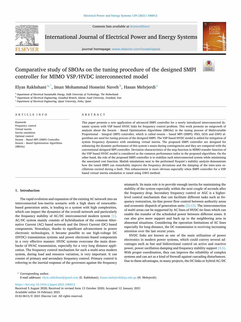
Fig. 10. Variation of input signals: (a). Δu1, (b). Δu2.

Table 1 Setting The Same Parameters of SBOAs for VSP/HVDC Model.

Parameters Values

Number of Variables Lower Bound of Variables Upper Bound of Variables Maximum Number of Iterations Swarm (Population) Size

4 − 1 1 300 80

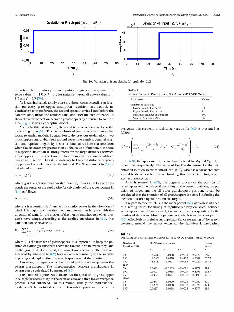
Table 2 Comparative transient performance for VSP/HVDC system, tuned by SMPI.

Number of Iterations PSO

SMPI Controller Gains Fitness Value

K1 K2 K3 K4 Z

50 − 4.2317 − 1.0338 − 0.9053 0.0770 845 100 − 2.8331 − 0.6518 − 0.0105 0.0081 202.5 150 − 1.1287 − 0.0801 − 0.0093 0.0020 197.3 GOA 50 0.0633 − 0.1023 − 0.0011 0.9971 719 100 0.0407 − 2.0698 − 0.0009 0.8092 192.7 150 0.0397 − 0.0501 − 0.0008 0.6190 121.1 GWO 50 0.0241 − 0.0339 − 0.0003 0.5088 43.1 100 0.0239 − 0.0338 − 0.0003 0.5079 42.0 150 0.0237 − 0.0338 − 0.0003 0.5079 41.5

E. Rakhshani et al.


10

Fig. 11. Cost function deviation in VSP/HVDC model using SI algorithms.

Fig. 12. Variation of Frequency in area 1 and 2 (p.u.): (a). Δɷ1, (b). Δɷ2.

E. Rakhshani et al.


11

Therefore, it is cleared that the first part in equation (63), which is related to summation term, will be focused on the position of other grasshoppers and finally performs the grasshopper interconnection in nature.

The other main part in (63), Td, points to the variation rate of the tendency for grasshoppers to fly towards the food source. Also as it was explained in above, the parameter c can simulate the decreasing process of grasshopper which is proceeded towards the food source. All existent parts in (63), Td and the summation part, are multiplied by the random values which create more random behavior for grasshoppers.

The obtained formulation in (63), by using the explained two terms can explore and exploit the search space. The required structure in the level tuning of exploration and exploitation for search agents is provided as follows:

c = cmax - lcmax - cmin

L(64)

As it is observed in (64), the maximum and minimum values for c are introduced by cmax and cmin respectively. Also the current of iteration is shown using l and L is the biggest number of iterations. By attention to (64), it is indicated that the number of iteration and the parameter c are related together in order to make balance between the exploration and exploitation process.

By considering to above explanations, it is obvious that the proposed model can enhance gradually grasshopper to fly towards a task. In grasshopper optimization algorithm, the grasshopper with best objec-tive value is assumed as the fittest grasshopper during optimization process. This rule can cause to keep the best solution in every iteration for GOA.

4.3. Grey wolf optimization algorithm (GWO)

Comprehensive analysis about the taken processes from nature, finally focused the scientists and researchers to the swarm – based life of grey wolf. These studies lead to appear a well - regarded optimization algorithm that is called GWO. According to the achieved researches, the social behavior of grey wolves has a hierarchical structure [52]. The main part of swarm – based algorithm in GWO imitates by the social interconnection of grey wolves in nature. Almost a crowd of wolves is classified into specified types of members according to the command level including α, β, δ and ɷ. The most presiding wolf is α and this ability will be reduced from α to ɷ. The hunt process in wolves usually performs as a crowd. In the other hand, wolves cooperate in a smart way to hunt a

prey (victim). At first, the hunt process is started by pursuing the prey by Grey wolves as a team. Then they attempt to surround it circularly. This strategy will be continued in order to increase the chance of hunt. A conceptual diagram from this process is indicated in Fig. 7.

Above diagram insists that various positions can be enhanced by attention to the location of the grey wolf (x , y) and the situations of the prey (x* , y*). This idea can be extended for more than the 2th dimen-sion. It can be possible to create a mathematical model as follows:

D→ = |C→ . X→p(iter) - X→(iter)| (65)

X→(iter + 1) = X→p(iter) - A→ . D→ (66)

In (65) and (66), X→(iter + 1) emphasizes on the new position of the wolf. Also X→p(iter), by subscript p, indicates to the current location of prey (victim).

According to above equations, For calculation of A→ and C→, as specified coefficients, the equations are presented by (67) and (68). It is obvious that the distance which relates to the location of the prey (victim), will be shown by D→.

A→ = 2. a→ . r→1 - a→ (67)

C→ = 2. r→2 (68)

where a→ is a tuning parameter that reduces linearly from 2 to 0 during the process. Also two random parameters, r→1 and r→2, are produced from the interval 0 to 1.

In the optimization process, the earliest three best solutions are selected and kept. Then the update process of their locations will be continued based on the best search agents. Finding a mathematical model for the hierarchical behavior formulation of wolves in enhance-ment of GWO algorithm, will be realized by classification their popu-lation into: α, β, δ and ɷ. Fig. 8 indicates the upgrade process of positions for α, β and δ, respectively, in a two-dimensional space.

The other nominee for solutions are focused on ɷ. Actually in GWO, the optimization process is managed by α, β, δ and ɷ. So by keeping the first three best obtained solutions so far and enforcing the other search agents (including the ɷ) to upgrade their positions based on the location of the best search agent. Also in this process, the main below equations are presented.

Fig. 13. Variation of tie line AC power between areas.

E. Rakhshani et al.


12

D→α = |C→1.X→

α − X→| (69)

D→β = |C→2.X→

β − X→| (70)

D→δ = |C→3.X→

δ − X→| (71)

X→1 = X→α − A→1.D→

α (72)

X→2 = X→β − A→2.D→

β (73)

X→3 = X→δ − A→3.D→

δ (74)

X→(iter + 1) =X→1 + X→2 + X→3

3(75)

In fact, this swarm – based algorithm will be completed using (69) – (75) and therefore the upgrade process of position is achieved based on to α, β and δ in a dimensional search space. In (67) and (68), A→ and C→

are enforced this process to explore and exploit the search space. Reducing A→ will be lead that half of the iterations is devoted to

exploration (A→ ≥ 1) and the other half is dedicated to exploitation (A→< 1). The variation of C→ is 0 ≤ C→≤ 2 and the vector C→ also modi-fied exploration when C→ > 1. Also for C→< 1, exploitation will be highlighted.

According to α, β and δ in a dimensional search space. In these for-mulas, A→ and C→ are obliging the GWO algorithm to explore and exploit the search space.

With decreasing A→, half of the iterations is devoted to exploration (A→≥ 1) and the other half is dedicated to exploitation (A→ < 1). The range of C→ is 0 ≤ C→≤ 2 and the vector C→ also improves exploration when C→> 1. Exploitation is emphasized when C→< 1.

5. Simulation results

This section is presented with two main parts. The first part is focused on preparation and cost function determination. The last part will focus on the desing of the controller, test and simulation. To eval-uate the performance of SBOAs in finding the best coefficients of multivariable PI (MPI) for VSP/HVDC model, at first, it is necessary to

Fig. 14. Variation of injected DC power in VSP1: (a). Δxp,vsp1, (b). Δxf,vsp1.

E. Rakhshani et al.


13

propose a new cost function according to desired MIMO characteristics. The applied minimization process will be achieved using SBOAs for the proposed cost function and it will be compared with the typical tuned SMPI based on Section. 3. Also for achieving a comprehensive com-parison between different models, the model with AC/HVDC system is also presented in an individual section and the proposed SMPI controller is performed and discussed.

Some of the main assumptions which are utilized in the simulation process of the proposed swarm – based optimization MPI (SMPI) controller are as follow:

a) To set up initial parameters for swarm – based optimization methods: Number of decision variables (nVar = 4).

Lower and upper bond of decision variables (VarMin = -1 and Var-Max = 1). Maximum number of iterations (MaxIt = 300). Population size (nPop = 80).

b) To set up VSP/HVDC model: AVSP, BVSP and CVSP as the constant state, input and output matrices. Implementation of input reference signal at r(t). Simulation time range is equal to 50 s.

5.1. Proposed cost function

In this section, it is necessary to select a specified approach among the optimization process. By attention to the determined features of step response and its accessibility in every iteration of the simulation, a fitness index is used according to the extracted features of the step function. So the calculation process of the cost function is performed according to the obtained MIMO transfer function in this part.

It should be noted that the proposed fitness index actually is a function, including summation of the selected step response features, which they are formulated as a linear combination by weighted co-efficients. The utilized features, which are mentioned in this work, are

Fig. 15. Variation of injected DC power in VSP2: (a). Δxp,vsp2, (b). Δxf,vsp2.

Table 3 The best performance index for SBOAs.

SBOA SMPI Controller Gains Fitness Value K1 K2 K3 K4 Z

PSO − 1.1203 − 0.0764 − 0.0017 0.0001 193.4070 GOA 0.0241 − 0.0343 − 0.0003 0.5142 41.7571 GWO 0.0237 − 0.0338 − 0.0003 0.5070 41.7507

E. Rakhshani et al.


14

defined as follow: 1. Stability Index (SI): The movement manner of closed – loop poles

as an effective parameter should be mentioned in simulations. As it is cleared, the pole position can be affected by the system’s stability. In this study, the most attention should be given to adding an equal index for

managing stability during the optimization process. To determine this component, at first it is important to find the real value of poles. After that, we can select the most positive value between the obtained reals while determining their maximum. It is noted that when these poles locate on the imaginary axes or in the right hand of s (unstable poles),

Fig. 16. Nyquist diagram for the VSP/HVDC transfer functions (GVSP(i, j)) using SBOAs , a)G11, b) G12, c) G21, d) G22.

E. Rakhshani et al.


15

the calculated parameter will be zero or bigger than zero. To overcome this problem, we can write:

MaxRealPole = min(max{Real(p1),Real(p2),⋯,Real(pi) }, 0 ) (76)

By attention to (76), the maximum real part of closed loop poles will be negative. Finally, the SI parameter can be defined as follows. It is obvious that the lower SI the better:

SI =-1

MaxRealPole(77)

In (76), p1, p2,…,pi are the obtained closed-loop poles. 2. Settling Time Index (ST): One of the most specified features for

step response in a system is the minimum time that the amplitude gets to correct error of 0.05. On the other hand, according to (20), VSP/HVDC model, as the basic system, has MIMO transfer function. Then by implementation of step unit function as the input signal, the obtained step response will be calculated as a 2 × 2 matrix. Therefore, in this work we will confront four ST parameters which every one of them belongs to one of the element matrices of the step response. On the other hand, it is clear that for MIMO step response:

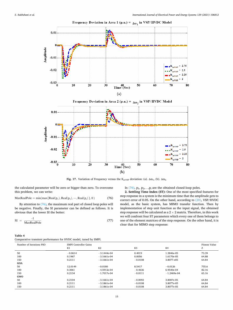
Fig. 17. Variation of Frequency versus the KacVSP deviation: (a). Δɷ1, (b). Δɷ2.

Table 4 Comparative transient performance for HVDC model, tuned by SMPI.

Number of Iterations PSO SMPI Controller Gains Fitness Value K1 K2 K3 K4 Z

50 − 0.0614 − 3.1444e-04 0.4019 1.3846e-05 73.39 100 0.1967 − 3.1661e-04 0.0056 1.6170e-05 64.88 150 0.2111 − 3.1661e-04 − 0.0108 3.8077-e05 64.84 GOA 50 12.0149 − 0.0180 8.5417 − 0.0126 755.6 100 0.3061 − 4.5912e-04 − 0.4636 6.9540e-04 82.16 150 0.2134 − 1.7017e-04 − 0.0111 − 1.2469e-04 65.16 GWO 50 0.2104 − 3.1661e-04 − 0.0092 3.8007e-05 64.84 100 0.2111 − 3.1861e-04 − 0.0108 3.8077e-05 64.84 150 0.2111 − 3.1861e-04 − 0.0108 3.8077e-05 64.84

E. Rakhshani et al.


16

STMIMO =

[ST11 ST12ST21 ST22

]

(78)

Eventually, by considering the worst possible situations, and the obtained elements of the matrix (78), this index can be determined by:

ST = max{

STij}

(79)

3. Rise Time Index (RT): The other effective feature of step response, can be determined as the time it takes for the response to rise from 10% to 90% of the steady-state response. Similarly, there is a

Fig. 18. Cost function deviation in HVDC model using SBOAs.

Fig. 19. Variation of Frequency in area 1 and 2 (p.u.) for HVDC model: (a). Δɷ1, (b). Δɷ2.

E. Rakhshani et al.


17

matrix for the determined RT as follows:

RTMIMO =

[RT11 RT12RT21 RT22

]

(80)

and finally this index will be calculated as:

RT = max{

RTij}

(81)

By notification to (77), (79) and (81), the cost function can be defined as a linear combination of above indexes:

Z = k1 × (SI) + k2 × (ST) + k3 × (RT) (82)

where k1, k2 and k3 are constant and real positive digits which are selected by attention to the target design. By definition of their values, we can change the role of every above index in the minimization of a cost function. It is notified that in this case, all ki are selected equal to 1. As it is indicated in (82), the fitness index is produced by three ho-mogenous terms with the same dimension. This important point is applied by selecting the manner of three indexes, including SI, ST and RT.

Therefore, SBOAs will be completed by implementing this cost function during the optimization procedure. Fig. 9 illustrates a con-ceptual process from the optimization method for the proposed cost

function. This task is achieved using swarm – based strategies. As shown in Fig. 9, the proposed optimization algorithm can be

performed as follows:

a) Set up Initial parameters for swarm – based optimization methods, consist of:

• Number of decision variables (nVar = 4). • Lower and upper bond of decision variables (VarMin = -1 and Var-

Max = 1). • Maximum number of iterations. • Population size (nPop = 80).

b) Selection of decision variables randomly and replacing in MPI structure as follows:

• Select (k1, k2, k3, k4).

• Perform the selected ki to

⎧⎪⎪⎪⎪⎨

⎪⎪⎪⎪⎩

GC1(s) = K1 +K2

s

GC2(s) = K3 +K4

s c) Calculate the closed loop transfer function by the obtained decision

variables from (b) and equations (23) – (32). d) Extract the proposed cost function terms, for achieving to SI, ST and

RT, by means of the obtained result from (c).

Fig. 20. Variation of Tie line AC power between areas (p.u.MW) for HVDC model.

Table 5 Comparison Analysis Between State Variables in The Tuning SMPI Process Using PSO.

VSP/HVDC Model

HVDC Model

Dynamical Model Time

Tie Line AC Power Deviation

Frequency Deviation in area 2




Frequency Deviation in area 1 Simulation time

ΔPtie,AC12 Δω2 Δω1 ΔPtie,AC12 Δω2 Δω1 t (Sec)¡ 0.0002633 ¡ 0.02158 − 0.006642 0.0007779 − 0.02452 ¡ 0.005311 5 0.0001133 − 0.00153 ¡ 0.002091 0.0001546 ¡ 0.00108 − 0.002293 10 1.521 £ 10-5 − 0.0002702 − 0.0007933 − 1.932 × 10-5 0.0002673 0.0003379 15 3.743 £ 10-6 ¡ 0.0001012 ¡ 0.0001009 − 6.326 × 10-6 0.0001015 0.0001102 20 5.182 £ 10-6 ¡ 8.936 £ 10-5 ¡ 1.414 £ 10-5 − 5.761 × 10-6 9.855 × 10-5 9.723 × 10-5 25 5.265 £ 10-6 ¡ 9.563 £ 10-5 ¡ 5.266 £ 10-5 − 5.888 × 10-6 9.962 × 10-5 9.958 × 10-5 30 − 0.000293 0.001664 0.001052 ¡ 0.000262 0.001555 0.005838 35 − 1.515 × 10-5 9.127 £ 10-5 5.373 £ 10-5 1.101 £ 10-5 − 9.768 × 10-5 − 5.614 × 10-5 40 ¡ 9.536 £ 10-7 4.053 £ 10-5 2.365 × 10-5 − 9.848 × 10-7 4.311 × 10-5 8.998 £ 10-6 45 − 3.108 × 10-6 5.221 £ 10-5 9.289 × 10-5 ¡ 3.094 £ 10-6 5.154 × 10-5 5.155 £ 10-5 50

E. Rakhshani et al.


18

e) Calculate the final cost function by replacing the obtained results from (d) into equation (82).

f) Consider the most important limitations in this process, as it follows: • Proper Local Minimizations: If the obtained cost function, according to

(82) in (e), before achieving to the optimal value, is fixed on a specified value and then this situation is continuously repeated more than 15 iterations.

• Stability limitations: It is important to stay all the obtained poles in the closed – loop transfer function on the left hand of S pane in all iterations.

• Possibility of realization: The industrial implementation of MPI controller will be related to the obtained actuator signal as U ac-cording to (22) and (34).

• Final Decision about above limitations: If every set of the selected Ki is lead to one of above limitations, that set will be deleted from the collection of solutions.

g) New Iteration = past Iteration + 1 h) If (new iteration < max iteration) then update parameters and go

back to (b) i) Show the last value for Z and MPI coefficients as follow:

K(s) =

[kp1 00 kp2

]

+1s

[kI1 00 kI2

]

(83)

j) End.”

5.2. Preparation process

By attention to Section 2, input signals for MIMO VSP/HVDC model are considered as (17) and Fig. 10 shows the variation of the input variables.

Namely, it is assumed that contingencies happened as step load

changes in the first area by rising to 0.03p.u. at t = 2 sec, and then the load value deviation becomes 0.015p.u. at t = 30 sec. Then for simu-lation of these step changes, r(t) can be defined as input signals:

r(t) = [ 1 -1 ][

Δu1Δu2

]

(84)

For high availability to all parameters and the obtained separated results in simulations, it is better to program as an extendable structure. As it was described in PSO algorithm, every particle can carry out structures, consisting of the position, objective value (cost value), ve-locity and the best structure. In the same way, the best structure will be included position and objective value (cost value) part too. This sepa-rated structure will be achieved on others SBOAs, such as GOA and GWO.

Table 1 shows common tuning parameters for all SBOAs. Additional parameters for different numbers of iteration with different algorithms are presented in Table 2 as well.

In this scenario, all parameters have to be designed and installed in a way that the gains of Ki (i = 1,2,3,4) in the below MPI controller can be calculated:

K(s) = KP +KI

s(85)

KP =

[K1 00 K2

]

(86)

KI =

[K3 00 K4

]

(87)

Table 6 Comparison Analysis Between State Variables in The Tuning SMPI Process Using GOA.

VSP/HVDC Model

HVDC Model








ΔPtie,AC12 Δω2 Δω1 ΔPtie,AC12 Δω2 Δω1 t (Sec)¡ 0.0007793 ¡ 0.02052 ¡ 0.01283 0.001203 − 0.03873 − 0.008351 5 9.829 £ 10-5 − 0.002521 ¡ 0.003881 0.0003597 ¡ 0.001676 − 0.005417 10 2.85 £ 10-5 − 0.0009589 0.0003677 − 4.713 × 10-5 0.0006717 0.0006767 15 2.648 × 10-5 0.0001535 0.0001323 ¡ 2.245 £ 10-5 0.000164 0.0002185 20 9.103 £ 10-6 0.0001137 0.0003630 − 9.112 × 10-6 0.0001587 0.0001551 25 9.257 £ 10-6 0.0001327 0.000273 − 9.704 × 10-6 0.0001645 0.0001640 30 ¡ 7.525 £ 10-5 0.003587 0.00363 − 0.0004688 0.003801 0.009911 35 1.161 × 10-5 0.0002018 8.237 £ 10-5 1.135 × 10-5 − 0.000206 − 8.785 × 10-5 40 5.421 £ 10-7 4.154 £ 10-5 2.156 £ 10-5 8.34 × 10-7 4.642 × 10-5 − 2.192 × 10-5 45 5.113 £ 10-6 8.116 £ 10-5 8.117 £ 10-5 − 5.319 × 10-6 8.82 × 10-5 8.855 × 10-5 50

Table 7 Comparison Analysis between State Variables in The Tuning SMPI Process Using GWO.

VSP/HVDC Model

HVDC Model








ΔPtie,AC12 Δω2 Δω1 ΔPtie,AC12 Δω2 Δω1 t (Sec)¡ 0.0002613 ¡ 0.02138 − 0.006622 0.0007739 − 0.02432 ¡ 0.005301 5 0.0001103 − 0.00151 ¡ 0.002051 0.0001516 ¡ 0.00105 − 0.002283 10 1.501 £ 10-5 − 0.0002701 − 0.0007903 − 1.902 × 10-5 0.0002653 0.0003329 15 3.713 £ 10-6 ¡ 0.0001002 ¡ 0.0001001 − 6.316 × 10-6 0.0001005 0.0001101 20 5.132 £ 10-6 ¡ 8.916 £ 10-5 ¡ 1.404 £ 10-5 − 5.721 × 10-6 9.315 × 10-5 9.523 × 10-5 25 5.225 £ 10-6 ¡ 9.533 £ 10-5 ¡ 5.236 £ 10-5 − 5.868 × 10-6 9.932 × 10-5 9.658 × 10-5 30 − 0.000291 0.001644 0.001032 ¡ 0.000242 0.001525 0.005818 35 − 1.505 × 10-5 9.107 £ 10-5 5.343 £ 10-5 1.081 £ 10-5 − 9.748 × 10-5 − 5.612 × 10-5 40 ¡ 9.506 £ 10-7 4.013 £ 10-5 2.335 × 10-5 − 9.828 × 10-7 4.301 × 10-5 8.992 £ 10-6 45 − 3.102 × 10-6 5.201 £ 10-5 9.249 × 10-5 ¡ 3.054 £ 10-6 5.124 × 10-5 5.151 £ 10-5 50

E. Rakhshani et al.


19

Fig. 21. Nyquist diagram for the HVDC transfer functions (GHVDC(i, j)) using SBOAs; a)G11, b)G12, c)G21, d)G22.

E. Rakhshani et al.


20

5.3. First Scenario: Simulation of the designed SMPI for VSP/HVDC model

In this section, a VSP/HVDC model, as it was defined in Section 2, will be considered as the base test system to evaluate the achievement SMPI controller compared to a typical setting method. It is mentioned that two load step changes are happening at 3 sec and 30 s as shown in Fig. 10. The performance of the developed model is simulated by developing both MATLAB scripts and SIMULINK R2016b® environment which is a programming platform for numerical computation and data. For implementing SMPI with different SBOAs, PSO, GOA and GWO are designed and installed to calculate the gains of Ki (i = 1,2,3,4).

According to Fig. 9 and Section 5.1, basically, a MIMO matrix will be determined as the step response. Then the obtained features, including ST, SI and RT, are extracted and entered in the optimization algorithm.

Fig. 11 shows the variation of cost function value versus the number of iterations. In this figure, the cost function of deviations is illustrated based on SBOAs. According to Fig. 11, GWO scenario presents faster convergence by less iteration. Table. 2 can provide the possibility of comparison between different swarm – based intelligence methods and their convergence speed in the same situations. As it is observed, this comparison is applied in various population size. By considering the recorded values, the GWO and GOA characteristics are so closed and more suitable than PSO. Also the obtained PSO features are slower and farther than other two SBO algorithms. By comparison between the final cost function, it is obvious that the optimization process in GWO and GOA has achieved more accurate than PSO. So the obtained results in Table. 2, can satisfy the cost function deviation in Fig. 11.

For having a better comparison, the tuning process of tuning SMPI coefficients is applied with four SBOAs, consist of a typical tuned method, tuned using PSO, GOA and GWO strategy. For the first and the second state variables in VSP/HVDC model, Fig. 12 (a) and (b) exhibit the frequency deviations in area 1 and 2 (Δɷ1, Δɷ2) using typical tuned MPI controller method and the proposed SBOAs.

Based on the simulation results, it is clear that the conventional tuning method, presented in Section 3, has the least effect on output signal. Just the reverse of usual tuning method, Fig. 12 shows that the applied swarm-based tuning method can represent a more accurate performance from the old setting strategy. This fact is more cleared during the optimization process by means of GWO and GOA.

Fig. 13 discloses tie – line AC power between areas (ΔPtieAC12) de-viations in VSP – HVDC model. It is absolutely clear that ΔPtieAC12 is controlled by the acceptable damping using GWO versus other SBOAs basis on the simulation results.

Also in this case, the conventional MPI controller has more suitable performance than PSO. Convinces the precise performance of estimation stage too.

Fig. 14 (a) and (b) indicate the injected DC power deviation and its derivative in VSP1 for VSP/HVDC model (Δxp,vsp1 and Δxf,vsp1 respec-tively). In both (a) and (b), the SMPI controller design process has more suitable performance using GWO. Also the typical MPI tuning method has less direct effect on system without any controller.

It is clear that GOA has more closed results to GWO method. This conclusion is seen in all simulation results.

Fig. 15 (a) and (b) indicate the injected DC power deviation and its derivative in VSP2 for VSP/HVDC model (Δxp,vsp2 and Δxf,vsp2 respec-tively). In both, the SMPI controller design process has more suitable performance using GWO. The obtained values for the SMPI controller gains (KP and KI matrixes) with different SBOAs, consist of PSO, GOA and GWO, are given in Table. 3. Also the final performance index values for SBOAs are described in Table. 3.

5.3.1. Sensitivity analysis for VSP/HVDC case As it is obvious, the stability condition for a closed – loop structure is

described by this way that if and only if the trajectory of the Nyquist diagram of G(sjɷ)H (jɷ) from -∞ < ɷ < ∞ encircles the point (-1,0) in a

counter-clockwise direction as much times as G(s)H (s) has unstable poles.

Above explanation can be extended by the generalized Nyquist’s stability criterion for MIMO systems, which is a modification from the Nyquist’s stability criterion for SISO systems [53–54].

By attention to Section II and (20), the generalized Nyquist’s stability criterion for SBOAs, including PSO, GOA and GWO can be achieved by the below figures. From the obtained graphs in Fig. 16, it is observed that GWO and GOA methods are more stable than PSO tuning method. In this figure, the conventional MPI controller design is shown by the ’No Control’ legend.

5.3.2. Robustness analysis for VSP/HVDC case In this section, it is possible to analysis the behavior of the tuned

SMPI controller using GWO method, as the most optimal SBOAs on the VSP/HVDC model, against parameter changes. By considering a com-mon set – up parameter for both VSPs and a direct relation between selected parameter and tie – line AC power deviation among area 1 and 2, we can choose kacVPS as the most suitable parameter. In the other hand, we will able to study robustness analysis on VSP/HVDC model, as the structured uncertainty. Therefore, we present the reaction of Δɷ1, Δɷ2 and ΔPtieAC12 after applying this robust evaluation strategy. As it seems, by decreasing kacVSP from the standard value, frequency de-viations in both areas start to decrease step by step. This change is shown in Fig. 17. Therefore, as it is cleared, despite the implementation of kacVSP variations in VSP/HVDC model, the proposed SMPI controller stay in the stability range.

5.4. Second Scenario: Design of SMPI on AC/HVDC model

As it was described in the previous section, VSP/HVDC model, will be obtained by means of utilization a higher level control technique for emulation using VSP. In the other hand, this control structure performs by programming the electrical performance of a synchronous generator (SG) in a HVDC line which is responsible for controlling the VSC – converter. Therefore, every tuning on this model, such as tuning SMPI controller basis on this paper, as separately can impress the performance of HVDC model. So the second scenario will be centralized on the SMPI controller effects for HVDC model.

By attention to this model, the converter stations of the HVDC links in a multi - area AC/DC interconnected system, as a dynamic model of the facilitated MIMO system by means of following equations: ⎧⎪⎪⎨

⎪⎪⎩

ΔxHVDC(t) = AHVDC(10×10)ΔxHVDC(t) + BHVDC

(10×2)ΔuHVDC(t)

ΔyHVDC(t) = CHVDC(2×10)ΔxHVDC(t)

(88)

ΔxHVDC =

[Δω1 Δω2 ΔPm1 ΔPm2 ΔPm3 ΔPm4

ΔPref1 ΔPref2 ΔPtieAC12 ΔPDC

]T

(89)

ΔuHVDC = [ΔPl1 ΔPl2]T (90)

ΔyHVDC = [Δω1 Δω2]T (91)

Finally, by considering described equations, MIMO transfer function for HVDC model can be driven as follows:

GHVDCTotal (s) = CHVDC

(2×10)

(SI - AHVDC

(10×10)

)-1BHVDC

(10×2) (92)

[Δω1(s)Δω2(s)

]

=

[GHVDC

11 (s) GHVDC12 (s)

GHVDC21 (s) GHVDC

22 (s)

][ΔPL1(s)ΔPL2(s)

]

(93)

The MIMO transfer function in (92) for the AC/HVDC model shown in equation (93) considering its state space matrices is presented in Appendix A.

E. Rakhshani et al.


21

As it was mentioned for VSP/HVDC model, by considering to the same initial parameters for swarm – based optimization algorithms and the same load step change as input deviations, simulation results for HVDC model will be presented as follow:

By attention to Table. 4 and Fig. 18, it is observed that the cost function value for the tuning process using PSO method has performed so closed values to the output results using GWO method. Also in HVDC model, for the initial iterations, GOA method performs slowly but in the other iterations this method can compensate its backwardness suitably and tends to the same permanent value.

By attention to the obtained values for PI coefficients, (Ki, i =1,2,3,4), it seems that tuned SMPI controller in HVDC model tends to behave similar to a MP controller.

By considering Figs. 19 and 20, it is clear that the typical tuned MPI controller is slower than SMPI controllers (using PSO, GOA and GWO). Also it seems that the obtained results from the tuned SMPI controllers, using PSO and GWO, are more suitable than the proposed controller tuning by GOA.

The obtained simulation results from HVDC model can give the comparison opportunity to VSP/HVDC model. This comparison can perform by attention to the following tables for every swarm – based optimization algorithm. As it is observed, frequency deviation in both two – areas and tie line AC power deviation between areas, as the same state variables, are selected from both models and then they are compared in 10 sample time, with 5 s for every range time. These tables can represent the comparison ability for finding the leveling effect of utilization swarm – based optimization algorithms in the tuning process of MPI controller.

By attention to Table. 5, 6 and 7, it is observed that the obtained simulation results in the SMPI tuning process from VSP/HVDC model are closer to zero value and then all swarm – based optimization algorithms, PSO and GOA and GWO, have more suitable values for VSP/HVDC model.

5.4.1. Sensitivity analysis for AC/HVDC model As it was illustrated in the first scenario. In this section and about

HVDC model, we can utilize the generalized Nyquist’s stability criterion for the second scenario’s model.

Therefore, the sensitivity analysis frequency for SBOAs, including PSO, will be obtained by the below figures. Fig. 21 presents Nyquist stability for all four transfer functions elements in GHVDC

Total from (93). From this figure, it is obvious that the tuning methods, including PSO and GWO, perform so closed and they can create a suitable performance for SMPI controller. Absolutely, the GOA method creates more sensitive Nyquist diagram which is related to be weaker its performance in comparison with two other SBOAs.

6. Conclusion

A new high-level control application for a heuristic-based multivar-iable PI (MPI) controller design for an interconnected dynamic AGC model with VSP is presented and discussed.

Swarm-based optimization algorithms (SBOAs), as the most applied, natural – based and flexible meta – heuristic methods, is utilized to achieve the optimized solution where exact optimization techniques fail to obtain the satisfying results. In this work, it is tried to make a new

challenge for comparative analysis SBOAs and their performance to adjust a Multivariable PI (MPI) controller, which is called Swarm - Based Multivariable PI (SMPI) controller. By considering more experienced background in the optimization problems, recently applied researches and well-known structure in scientific societies, particle swarm opti-mization (PSO), grasshopper algorithm (GOA) and also grey wolf opti-mization (GWO) are mentioned, among all SBOAs, to implement in this tuning MPI process. These selected SBOAs are set – up and tested on a multi – input multi output (MIMO) AGC model with high voltage direct current (HVDC) with the virtual synchronous power (VSP) strategy, which is called VSP/HVDC model. The proposed method is based on the minimization of a performance index, which is designed by considering the transfer function characteristics matrix in a MIMO system. The SMPI controller design method is performed for the systems to improve characteristics performance of the model versus the conventional MPI controller method. For achieving to the best comparison between methods:

1- A conventional tuning method is selected to design MPI gains, consist of KP and KI matrix, in VSP/HVDC model.

2- A performance index is selected based on the step response infor-mation, especially important characteristics such as settling time (ST), stability index (SI) and rise time (RT) are considered to mini-mize using SBOAs.

3- Set–up parameters for SBOAs, consist of PSO, GOA and GWO, are tried to be close together for more accurate comparison between methods.

4- The obtained results exhibit that the proposed SBOAs, especially GWO and GOA, have more suitable performance than the conven-tional tuning method.

It should be noted that in the presented study PSO has been selected the base swarm-based optimization algorithm for comparing with other methods. GOA is selected at one of the newest intelligent algorithm among the other. Respect with other existing methods, application of other swarm based algorithms, such as monarch butterfly optimization (MBO), earthworm optimization algorithm (EWA), elephant herding optimization (EHO), can be considered as part of our future research.

Performed studies show that the proposed controller has few pa-rameters to adjust and is relatedly simple to implement. Its robust and can be used in parallel computation. The speed of its convergence for the studies cases are fast with short computational time. But despite of the advantages, it is important to take into account the importance of initial designed parameters. Improper values for the initial parameters might lead to premature convergence reaching to a local minimum especially with very big system with high complexities. The industrial imple-mentation of MPI controller will be related to the obtained actuator signal as U, shown in equation (22), and during the design process it is important to stay all the obtained poles in the closed – loop transfer function on the left hand of S-plan in all iterations.

Declaration of Competing Interest

The authors declare that they have no known competing financial interests or personal relationships that could have appeared to influence the work reported in this paper.

Appendix A

Calculated MIMO transfer function for VSP/HVDC model by attention to its state space model with calculation matrixes Avsp, Bvsp and Cvsp.

E. Rakhshani et al.

InternationalJournalofElectricalPowerandEnergySystems129(2021)106812

22

Gvsp11 (s) =

-6 s (s + 24.56) (s + 2.684) (s + 2.634)2(s + 1.982) (s + 1.939) (s + 0.5735) (s2 + 0.05763s + 0.001989) (s2 + 0.1409s + 0.4298)

(s + 2.684) (s + 2.632) (s + 1.99) (s + 1.255) (s + 0.6608) (s + 0.04727) (s + 0.008753) (s2 + 2.175s + 1.337) (s2 + 0.4635s + 0.4125)(s2 + 25.33s + 177.4)

Gvsp12 (s) =

-1.5891 s (s + 24.56) (s + 2.683) (s + 2.631)2(s + 1.939) (s2 + 0.06155s + 0.001975) (s2 + 2.659s + 1.858)

(s + 2.684) (s + 2.632) (s + 1.99) (s + 1.255) (s + 0.6608) (s + 0.04727) (s + 0.008753) (s2 + 2.175s + 1.337) (s2 + 0.4635s + 0.4125)(s2 + 25.33s + 177.4)

Gvsp21 (s) =

-352.93 s (s + 2.778) (s + 2.631) (s + 2.564) (s + 0.04458) (s + 0.01086) (s2 + 1.776s + 0.8746) (s2 + 2.632s + 1.842)(s + 2.684) (s + 2.632) (s + 1.99) (s + 1.255) (s + 0.6608) (s + 0.04727) (s + 0.008753) (s2 + 2.175s + 1.337) (s2 + 0.4635s + 0.4125)(s2 + 25.33s + 177.4)

Gvsp22 (s) =

-4.8 s (s + 2.778) (s + 2.632) (s + 2.564) (s + 1.258) (s + 0.3946) (s + 0.04458) (s + 0.01086) (s2 + 2.18s + 1.343)(s2 + 25.34s + 177.7)(s + 2.684) (s + 2.632) (s + 1.99) (s + 1.255) (s + 0.6608) (s + 0.04727) (s + 0.008753) (s2 + 2.175s + 1.337) (s2 + 0.4635s + 0.4125)(s2 + 25.33s + 177.4)

E. Rakhshani et al.


23

Calculated MIMO transfer function for AC/HVDC model by attention to its state space model with calculation matrixes Avsp, Bvsp and Cvsp.

GHVDC11 (s) =

-6 s (s + 25.52) (s + 2.681) (s + 2.631)2(s + 1.81) (s + 0.9308) (s2 - 0.5613s + 1.623)

(s + 23.73) (s + 2.683) (s + 2.632) (s + 0.9605) (s2 + 3.461s + 3.02) (s2 + 0.875s + 0.401) (s2 + 1.351s + 3.654)

GHVDC12 (s) =

-217.58 s (s + 2.681) (s + 2.634)2(s + 1.036) (s2 + 2.659s + 1.858)

(s + 23.73) (s + 2.683) (s + 2.632) (s + 0.9605) (s2 + 3.461s + 3.02) (s2 + 0.875s + 0.401) (s2 + 1.351s + 3.654)

GHVDC21 (s) =

70.419 s (s + 3.2) (s + 2.778) (s + 2.631) (s + 2.564) (s2 + 2.632s + 1.842)(s + 23.73) (s + 2.683) (s + 2.632) (s + 0.9605) (s2 + 3.461s + 3.02) (s2 + 0.875s + 0.401) (s2 + 1.351s + 3.654)

GHVDC22 (s) =

-4.8 s (s + 23.12) (s + 2.778) (s + 2.634) (s + 2.564) (s + 1.765) (s + 0.8017) (s2 + 1.99s + 2.642)(s + 23.73) (s + 2.683) (s + 2.632) (s + 0.9605) (s2 + 3.461s + 3.02) (s2 + 0.875s + 0.401) (s2 + 1.351s + 3.654)

References

[1] Tielens P, Van Hertem D. The relevance of inertia in power systems Renewable and Sustainable Energy Reviews. Renew Sustain. Energy Rev 2016:999–1009.

[2] Kunder P. Power System Stability and Control’. USA: McGraw-Hill; 1994. [3] Saadat H. Power system Analysis. McGraw-Hill; 1999. [4] Al-Haiki ZE, Shaikh-Nasser AN. Power Transmission to Distant Offshore Facilities.

IEEE Transactions on Industry Applications 2011;47:3. [5] Fan L, Miao Z, Osborn D. Wind farms with HVDC delivery in Load Frequency

Control. IEEE Transactions on Power Systems 2009;24:4. [6] Du Cuiqing E, Agneholm GO. Use of VSC- VDC for industrial systems having onsite

generation with frequency control. IEEE Trans. On Power Delivery 2008;23(4): 2233–40.

[7] Li Y, Zhanga Z, Yang Y, Li Y, Chenc H, Xua Z. Coordinated control of wind farm and VSC–HVDC system using capacitor energy and kinetic energy to improve inertia level of power systems. Electrical Power and Energy Systems 2014;59:79–92.

[8] L. Zhang, L. Harnefors and H.-P. Nee.: ’Power-synchronization control of gridconnected voltage-source converters’. IEEE Transactions on Power Systems, vol. 25, pp. 809-820, May 2010.

[9] Rodriguez P, Ignacio Candela J, Luna A. Control of PV Generation Systems using a Synchronous Power Controller’. ECCE, USA: IEEE Energy Conversion Congress and Exposition; 2013.

[10] Rodriguez P, Candela I, Citro C, Rocabert J, luna A. Control of grid-connected power converters based on a virtual admittance control loop’. Proc. 15th European Conference on Power Electronics and Applications (EPE) 2013.

[11] Rakhshani E, Remon D, Cantarellas AM, Garcia JM, Rodriguez P. Virtual Synchronous Power Strategy for Multiple HVDC Interconnections of Multi-Area AGC Power Systems. IEEE Transactions on Power Systems 2017;32(3):1665–77.

[12] S. J. Gambhire, D. Ravi Kishore, P. S. Londhe and S. N. Pawar. ’’Review of sliding mode based control techniques for control system applications’’. International Journal of Dynamics and Control. May 2020.

[13] Xinyu Zhang, Gun Li and Jin jun Shan. ’’Continuous PID-SMC based on improved EHGO for robot manipulators with limited state measurements’’. https://doi.org/ 10.1016/j.jfranklin.2020.09.001. Sep 2020.

[14] Waqas Anjum, Abdul Rashid Husain, Junaidi Abdul Aziz, M. Abbas Abbasi andHasan Alqaraghuli. ’’Continuous dynamic sliding mode control strategy of PWM based voltage source inverter under load variations’’. https://doi.org/ 10.1371/journal.pone.0228636. Feb 2020.

[15] Coelho LDS, Pessoa MW. A tuning strategy for multivariable PI and PID controllers using differential evolution combined with chaotic Zaslavskii map. Expert Systems with Applications 2011;38(11):13694–701.

[16] Ang KH, Chong G, Li Y. PID control system analysis, design, and technology. IEEE Transactions on Control Systems Technology 2005;13(4):559–76.

[17] Ho WK, Lee TH, Gan OP. Tuning of multiloop proportional-integral-derivative controllers based on gain and phase margin specifications. Industrial and Engineering Chemistry Research 1997;36(6):2231–8.

[18] Kumar VV, Rao VSR, Chidambaram M. Centralized PI controllers for interacting multivariable processes by synthesis method. ISA Transactions 2012;51(3):400–9.

[19] Sarma JKLN, Chidambaram M. ’Centralized PI/PID controllers for nonsquare systems with RHP zeros’. Indian Institute of. Science 2005;85(4):201–14.

[20] Montazar A, Van Overloop PJ, Brouwer R. Centralized controller for the Narmada main canal. Irrigation and Drainage 2005;54(1):79–89.

[21] F. Morilla, F. Vazquez, and J. Garrido.: ’Centralized PID control by decoupling for TITO processes’. in Proceedings of the 13th IEEE International Conference on Emerging Technologies and Factory Automation (ETFA ’08), pp. 1318 –1325, Hamburg, Germany, September 2008.

[22] J. Garrido, F. Morilla, and F. Vazquez.: ’Centralized PID control by decoupling of a boiler-turbine unit’. in Proceedings of the European Control Conference, pp. 4007–4012, Budapest, August 2009.

[23] M. Willjuice Iruthayarajan and S. Baskar.: ’Covariance matrix adaptation evolution strategy based design of centralized PID controller’. Expert Systems with Applications, vol. 37, no. 8, 2010.

[24] Y. Lee, S. Park, and M. Lee.: ’PID controller tuning to obtain desired closed loop responses for cascade control systems’. Industrial and Engineering Chemistry Research, vol. 37, no. 5, 1998.

[25] Ahmad Taher Azar, Abdelrahman Sayed Sayed, Abdalla Saber Shahin. Hassan Ashraf Elkholy and Hossam Hassan Ammar. ’’PID Controller for 2-DOFs Twin Rotor MIMO System Tuned with Particle Swarm Optimization’’. DOI: 10.1007/ 978-3-030-31129-2_22. Jan 2020.

[26] Azar Ahmad Taher, AliEmail Nourhan, Makarem Sarah, Ammar Hossam Hassan. Design and Implementation of a Ball and Beam PID Control System Based on Metaheuristic Techniques 2020. https://doi.org/10.1007/978-3-030-31129-2_29.

[27] Jha Amitkumar V, Gupta Deepak Kumar, Appasani Bhargav. The PI Controllers and its optimal tuning for Load Frequency Control (LFC) of Hybrid Hydro-thermal Power Systems 2020. https://doi.org/10.1109/ICCES45898.2019.9002150.

[28] Ghusn Abdul Redha Ibraheem, Ahmad Taher Azar, Ibraheem Kasim Ibraheem and Amjad J. Humaidi. ’’A Novel Design of a Neural Network-Based Fractional PID Controller for Mobile Robots Using Hybridized Fruit Fly and Particle Swarm Optimization’’. https://doi.org/10.1155/2020/3067024 . Apr 2020.

[29] Kanagavel Rameshkumar and Vairavasundaram Indragandhi. ’’Real Time Implementation and Analysis of Enhanced Artificial Bee Colony Algorithm Optimized PI Control algorithm for Single Phase Shunt Active Power Filter’’. Journal of Electrical Engineering & Technology. May 2020.

[30] Jennathu Beevi Sahul Hameed and Jayashree Ramasubramanian. ’’Optimal Fractional Order PI Controller for Frequency Ancillary Services in Restructured Power System’’. Journal of Energy Systems. May 2020.

[31] Emre Çelik. ’’Improved stochastic fractal search algorithm and modified cost function for automatic generation control of interconnected electric power systems’’. https://doi.org/10.1016/j.engappai.2019.103407. Feb 2020.

[32] Sarma KLN, Chidambaram M. Centralized PI/PID controllers for non-square systems with RHP zeros. Indian Institute of Science 2005;85(4):201–14.

[33] Montazar A, Van Overloop PJ, Brouwer R. Centralized controller for the Narmada main canal. Irrigation and Drainage 2005;54(1):79–89.

[34] F. Morilla, F. Vazquez, and J. Garrido, “Centralized PID control by decoupling for TITO processes”. in Proceedings of the 13th IEEE International Conference on Emerging Technologies and Factory Automation (ETFA ’08), pp. 1318–1325, Hamburg, Germany, September 2008.

[35] J. Garrido, F. Morilla, and F. Vazquez, “Centralized PID control by decoupling of a boiler-turbine unit”. in Proceedings of the European Control Conference, pp. 4007–4012, Budapest, Hungary, August 2009.

[36] Willjuice Iruthayarajan M, Baskar S. Covariance matrix adaptation evolution strategy based design of centralized PID controller. Expert Systems with Applications 2010;37(8):5775–81.

[37] Mahdi Abachizadeh, Mohammad Reza Haeri Yazdi and Aghil Yousefi-Koma. ’’Optimal tuning of PID controllers using Artificial Bee Colony algorithm’’. DOI: 10.1109/AIM.2010.5695861. Jan 2011.

[38] M. Aabid, A. Elakkary and N. Sefiani . ’’PID parameters optimization using ant- colony algorithm for human heart control’’. DOI: 10.23919/ IConAC.2017.8082042. Oct 2017.

[39] Youssef Dhieb, Mohamed Yaich, Abdessatar Guermazi and Moez Ghariani. ’’PID Controller Tuning using Ant Colony Optimization for Induction Motor’’. Journal of Electrical Systems. March 2019.

[40] Qiu Shuang, Rui Xu, Zhai Tianchen. Anshuang Fu and Dong Ming. “Ant Colony Optimization Tuning PID Algorithm for Precision Control of. Functional Electrical Stimulation“. 2013. https://doi.org/10.1515/bmt-2013-4017. Sep.

[41] E. Rakhshani, P. R. Cortes.: ’Inertia Emulation in AC/DC Power Systems Using Derivative Technique Considering Frequency Measurement Effects’. IEEE Transactions on Power Systems, Volume: 32, Issue: 5, 2017.

[42] Rakhshani E, Remon D, Mir Cantarellas A, Rodriguez P. Analysis of derivative control based virtual inertia in multi-area high-voltage direct current interconnected power systems. IET Gener. Transm. Distrib. 2016;10(6):1458–69.

[43] Harris CJ. Self – Tuning and Adaptive Control: Theory and Applications. IEEE Control Engineering Series 1984.

[44] J. Penttinen and H. N. Koivo.: ’Multivariable Tuning Regulators for Unknown Systems’. Automatica, Vol. 16, pp 393-398, 1980.

[45] B. K. Panigrahi, Y. Shi, and M.H. Lim.: ’Handbook of Swarm Intelligence. Series: Adaptation, Learning, and Optimization’. Vol 7, Springer-Verlag Berlin Heidelberg, ISBN 978-3-642-17389-9, 2011.

[46] Blum C, Merkle D. Swarm Intelligence – Introduction and Applications. Springer, Berlin: Natural Computing; 2008.

E. Rakhshani et al.

http://refhub.elsevier.com/S0142-0615(21)00052-1/h0005





































https://doi.org/10.1007/978-3-030-31129-2_29

https://doi.org/10.1109/ICCES45898.2019.9002150








https://doi.org/10.1515/bmt-2013-4017. Sep









24

[47] M. Belal, J. Gaber, H. El-Sayed, and A. Almojel.: ’Swarm Intelligence’. In Handbook of Bioinspired Algorithms and Applications. Series: CRC Computer & Information Science. Vol. 7. Chapman & Hall Eds, ISBN 1-58488-477-5. 2006.

[48] Eberhart R, Kennedy J. A New Optimizer Using Particle Swarm Theory. Proc. 6th Symp. Micro 1995:29–43.

[49] Saremi Sh, Mirjalili S, Lewis A. Grasshopper ptimisation Algorithm: Theory and application. Advances in Engineering Software. ELSEVIER 2017:30–47.

[50] A. Lewis.: ’Low Cost: a spatial social network algorithm for multi - objective optimisation’. In: Evolutionary computation, CEC’09. IEEE congress, pp. 2866–2870.

[51] S. Mirjalili, M. Mirjalili and A. Lewis.: ’Greywolf optimizer’. Advances in Engineering Software, pp. 46–61, 2014.

[52] Skogestad S, Postlethwaite I. Multivariable Feedback Control Analysis and Design. Wiley Publications 2005.

[53] Johansson KH. Interaction Bounds in Multivariable Control Systems. Automatica 2002:1045–51.

E. Rakhshani et al.









Comparative study of SBOAs on the tuning procedure of the ...

Documents

Transcript of Comparative study of SBOAs on the tuning procedure of the ...